The Hermite-Taylor Correction Function Method for Embedded Boundary and Maxwell’s Interface Problems

Abstract

We propose a novel Hermite-Taylor correction function method to handle embedded boundary and interface conditions for Maxwell’s equations. The Hermite-Taylor method evolves the electromagnetic fields and their derivatives through order $m$ in each Cartesian coordinate. This makes the development of a systematic approach to enforce boundary and interface conditions difficult. Here we use the correction function method to update the numerical solution where the Hermite-Taylor method cannot be applied directly. The proposed high-order method offers a flexible systematic approach to handle embedded boundary and interface problems, including problems with discontinuous solutions at the interface. This method is also easily adaptable to other first order hyperbolic systems.

1 Introduction

Interface and boundary problems are of great importance in electromagnetics. The former type of problem involves interfaces between different media and is found in many applications in electromechanics, biophotonics and magneto-hydrodynamics, to name a few. The latter type of problem focuses on the interaction between the electromagnetic fields and a surface, and is found in waveguide applications.

In computational electromagnetics, many challenges arise from those types of problems. The development of efficient high-order methods are important to diminish the phase error for long time simulations Hesthaven2003 . This is particularly difficult for interface problems where the solution can be discontinuous at the interface. In addition to high-order accuracy, a numerical method should also be able to handle complex geometries.

Many high-order numerical methods have been developed to handle Maxwell’s interface and boundary problems, such as finite-difference time-domain (FDTD) methods Ditkowski2001 ; Cai2003 ; Zhao2004 ; Zhang2016 ; Banks2020 ; LawNave2022 , discontinuous Galerkin (DG) methods cockburn2001runge ; Hesthaven2002 and pseudo-spectral methods Yang1997 ; Driscoll1999 ; Fan2002 ; Galagusz2016 , to name a few.

In this work, we focus on the Hermite-Taylor method, introduced by Goodrich, Hagstrom and Lorenz in 2005 Goodrich2005 . This high-order method is particularly well-suited for linear hyperbolic problems on periodic domains. By evolving in time the variables and their derivatives through order $m$ in each coordinate, the Hermite-Taylor method achieves a $(2\,m+1)$ rate of convergence. The stability condition of this method depends only on the largest wave speed of the problem and is independent of the order of accuracy, making the Hermite-Taylor method appealing for large scale problems.

The difficulty in designing a systematic approach to handle the boundary conditions has prevented the use of the Hermite-Taylor method for many engineering and real-world scientific problems. Hybrid DG-Hermite methods were proposed to circumvent this issue by taking advantage of a DG method to handle the boundary conditions on complex geometries Chen2010 ; OversetHermiteDG . A DG solver is used on an unstructured or boundary fitted curvilinear mesh which encloses a Cartesian mesh where the Hermite method is applied. A local time-stepping procedure is needed to retain the large time-step sizes of the Hermite method.

Another method based on compatibility boundary conditions was developed for the wave equation on Cartesian and curvilinear meshes compat_wave_hermite_AAL_DEAA_WDH . In $d$ dimensions, this method computes the $(m+1)^{d}$ degrees of freedom on the boundary by enforcing the physical boundary condition as well as the compatibility boundary conditions. However, the extension of this method to first order hyperbolic systems is not straightforward.

In LawAppelo2022 , the Hermite-Taylor correction function method was proposed to handle general boundary conditions for Maxwell’s equations. This method relies on the correction function method (CFM) to update the numerical solution and its derivatives where the Hermite-Taylor method cannot be applied.

The CFM was first developed to enhance finite-difference methods for Poisson’s equation with interface conditions Marques2011 ; Marques2017 . It has been extended to the wave equation Abraham2018 and Maxwell’s equations LawMarquesNave2020 ; LawNave2021 ; LawNave2022 .

The correction function method seeks space-time polynomial approximations of the solution in small domains, called local patches, near the boundary or the interface by minimizing a functional. The functional is based on a square measure of the residual of the governing equations, boundary or interface conditions and the numerical solution from the original method (here the Hermite-Taylor method).

The CFM minimization procedure provides polynomial approximations, also called correction functions, that are used to compute the $(m+1)^{d}$ degrees of freedom at the nodes where the Hermite-Taylor method cannot be applied. The Hermite-Taylor correction function method presented in LawAppelo2022 achieved up to a fifth-order rate of convergence with a loose CFL constant, but was limited to boundaries aligned with the nodes.

This work extends the Hermite-Taylor correction function method to embedded boundary and interface problems. The paper is organized as follows. We introduce Maxwell’s equations with boundary and interface conditions in Section 2. The Hermite-Taylor method in two dimensions is presented in detail in Section 3. The correction function method in the Hermite-Taylor setting for embedded boundary and interface problems is described in Section 4. Finally, in Section 5, numerical examples in one and two dimensions, including problems with discontinuous electromagnetic fields, are performed to verify the properties of the Hermite-Taylor correction function method.

2 Problem Definition

In this work, we are seeking numerical solutions to Maxwell’s equations

$$\mu(\mathbold{x})\,\partial_{t}\mathbold{H}+\nabla\times\mathbold{E}= \,\,0,$$ (1)

$$\epsilon(\mathbold{x})\,\partial_{t}\mathbold{E}-\nabla\times\mathbold{H}= \,\,0,$$

$$\nabla\cdot(\epsilon(\mathbold{x})\,\mathbold{E})= \,\,0,$$

$$\nabla\cdot(\mu(\mathbold{x})\,\mathbold{H})= \,\,0,$$

in a domain $\Omega\subset\mathbb{R}^{d}$ ($d=1,2$) and a time interval $I=[t_{0},t_{f}]$. Here $\mathbold{H}$ is the magnetic field, $\mathbold{E}$ is the electric field, $\mu(\mathbold{x})>0$ is the magnetic permeability and $\epsilon(\mathbold{x})>0$ is the electric permittivity. The initial conditions are given by

$$\mathbold{H}(\mathbold{x},0)= \,\,\mathbold{H}_{0}(\mathbold{x})\quad\text{in }\Omega,$$ (2)

$$\mathbold{E}(\mathbold{x},0)= \,\,\mathbold{E}_{0}(\mathbold{x})\quad\text{in }\Omega,$$

and the boundary condition is given by

$$\mathbold{n}\times\mathbold{E}=\mathbold{g}(\mathbold{x},t)\quad\text{on }\partial\Omega\times I.$$ (3)

Here $\partial\Omega$ is the boundary of the domain $\Omega$, $\mathbold{n}$ is the outward unit normal to $\partial\Omega$ and $\mathbold{g}(\mathbold{x},t)$ is a known function.

We also consider Maxwell’s interface problems. In this situation, the domain $\Omega$ is subdivided into two subdomains $\Omega^{+}$ and $\Omega^{-}$, and is such that $\Omega=\Omega^{+}\cup\Omega^{-}$ and $\Omega^{+}\cap\Omega^{-}=\Gamma$. Here $\Gamma$ is the interface between the subdomains. Fig. 1 illustrates a typical geometry of a domain $\Omega$.

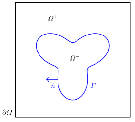
Figure 1: Geometry of a domain $\Omega$. The domain consists of two materials.

The physical parameters are assumed to be piecewise constant and are given by

$$\mu(\mathbold{x})=\left\{\begin{array}[]{l}\mu^{+}\quad\mbox{for}\quad\mathbold{x}\in\Omega^{+},\\[1.0pt] \mu^{-}\quad\mbox{for}\quad\mathbold{x}\in\Omega^{-},\end{array}\right.$$

and

$$\epsilon(\mathbold{x})=\left\{\begin{array}[]{l}\epsilon^{+}\quad\mbox{for}\quad\mathbold{x}\in\Omega^{+},\\[1.0pt] \epsilon^{-}\quad\mbox{for}\quad\mathbold{x}\in\Omega^{-}.\end{array}\right.$$

To complete Maxwell’s equations, we impose the interface conditions

$$\hat{\mathbold{n}}\times\llbracket\mathbold{E}\rrbracket= \,\,0\quad\text{on }\Gamma\times I,$$ (4)

$$\hat{\mathbold{n}}\times\llbracket\mathbold{H}\rrbracket= \,\,0\quad\text{on }\Gamma\times I,$$

$$\hat{\mathbold{n}}\cdot\llbracket\epsilon\,\mathbold{E}\rrbracket= \,\,0\quad\text{on }\Gamma\times I,$$

$$\hat{\mathbold{n}}\cdot\llbracket\mu\,\mathbold{H}\rrbracket= \,\,0\quad\text{on }\Gamma\times I.$$

Here $\llbracket\mathbold{H}\rrbracket=\mathbold{H}^{+}-\mathbold{H}^{-}$ is the jump of the variable $\mathbold{H}$ on the interface, $\mathbold{H}^{+}$ is the solution in $\Omega^{+}$, $\mathbold{H}^{-}$ is the solution in $\Omega^{-}$ and $\mathbold{\hat{n}}$ is the unit normal to the interface $\Gamma$.

3 Hermite-Taylor Method

In this section, we briefly describe the Hermite-Taylor method, introduced by Goodrich et al. in 2005 Goodrich2005 , to handle linear hyperbolic problems. For simplicity, the Hermite-Taylor method is presented in 2-D using the transverse magnetic (TM_z) mode. In this situation, Maxwell’s equations are simplified to

$$\mu\,\partial_{t}H_{x}+\partial_{y}E_{z}= \,\,0,$$ (5)

$$\mu\,\partial_{t}H_{y}-\partial_{x}E_{z}= \,\,0,$$

$$\epsilon\,\partial_{t}E_{z}-\partial_{x}H_{y}+\partial_{y}H_{x}= \,\,0,$$

$$\partial_{x}H_{x}+\partial_{y}H_{y}= \,\,0,$$

in a domain $\Omega=[x_{\ell},x_{r}]\times[y_{b},y_{t}]$ and a time interval $I=[t_{0},t_{f}]$. Here we assume the physical parameters $\mu$ and $\epsilon$ to be constant. We consider initial conditions on $H_{x}$, $H_{y}$ and $E_{z}$, and periodic boundary conditions.

The Hermite-Taylor method uses a mesh that is staggered in space and time. The primal mesh is defined as

$$(x_{i},y_{j})=(x_{\ell}+i\,\Delta x,y_{b}+j\,\Delta y),\quad i=0,\dots,N_{x},\quad j=0,\dots,N_{y},$$

with

$$\Delta x=\frac{x_{r}-x_{\ell}}{N_{x}},\quad\Delta y=\frac{y_{t}-y_{b}}{N_{y}}.$$

Here $N_{x}$ and $N_{y}$ are respectively the number of cells in the $x$ and $y$ directions. The numerical solution on the primal mesh is centered at times

$$t_{n}=t_{0}+n\,\Delta t,\quad n=0,\dots,N_{t},\quad\Delta t=\frac{t_{f}-t_{0}}{N_{t}}.$$

Here $N_{t}$ is the required number of time steps to reach $t_{f}$. The nodes of the dual mesh are located at the cell centers of the primal mesh

$$(x_{i+1/2},y_{j+1/2})=(x_{\ell}+(i+1/2)\,\Delta x,y_{b}+(j+1/2)\,\Delta y),$$

for $i=0,\dots,N_{x}-1$, $j=0,\dots,N_{y}-1$, and at times

$$t_{n+1/2}=t_{0}+(n+1/2)\,\Delta t,\quad n=0,\dots,N_{t}-1.$$

The Hermite-Taylor method requires three processes:

• Hermite interpolation

  Let us consider a sufficiently accurate approximation of each electromagnetic field component, for example $E_{z}$, and its derivatives $\frac{\partial^{k+\ell}E_{z}}{\partial^{k}x\partial y^{\ell}}$, $k,\ell=0,\ldots,m$, on the primal mesh at time $t_{n}$. For each cell of the primal mesh and for each electromagnetic field component, we compute the unique degree $(2\,m+1)^{2}$ tensor-product polynomial satisfying the value and the given derivatives of the electromagnetic field components at the corners of the cell. The resulting polynomial is known as the Hermite interpolant.

• Recursion relation

  For each cell of the primal mesh and for each electromagnetic field, we identify the derivatives of the Hermite interpolant at the cell center as scaled coefficients. Expanding each scaled coefficient of the Hermite interpolant in time gives us a space-time polynomial, referred to as the Hermite-Taylor polynomial, approximating each electromagnetic field. We then enforce Maxwell’s equations and its derivatives at the cell center to obtain a recursion relation for the scaled coefficients of the Hermite-Taylor polynomials.

• Time evolution

  For each cell and for each electromagnetic field, we update the numerical solution on the dual mesh by evaluating the Hermite-Taylor polynomials at the cell center $(x_{i+1/2},y_{j+1/2})$ and time $t_{n+1/2}$.

Let us now describe the 2-D Hermite-Taylor method in more detail. From the initial conditions, we know all the electromagnetic fields and their derivatives through order $m$ in each coordinate on the primal mesh at time $t_{0}$.

In the situation where the derivatives cannot be easily computed, we project the initial solution in a polynomial space of degree at least $2\,m+1$ to maintain accuracy. To do so, for each electromagnetic field and for each primal node $(x_{i},y_{j})$, we define the spatial domain $[x_{i-1/2},x_{i+1/2}]\times[y_{j-1/2},y_{j+1/2}]$ and project the initial solution on the space of degree $(2\,m+2)^{2}$ tensor-product Legendre polynomials. We then approximate the required derivatives of each electromagnetic field at $(x_{i},y_{j})$ using the derivatives of the Legendre polynomials approximating the electromagnetic fields.

3.1 Hermite Interpolation in Two Dimensions

On each cell $[x_{i},x_{i+1}]\times[y_{j},y_{j+1}]$ of the primal mesh and for each variable, we are seeking the Hermite interpolant $p_{i+1/2,j+1/2}^{f}(x,y)$ of degree $2\,m+1$ that satisfies

$$\frac{\partial^{k+\ell}p_{i+1/2,j+1/2}^{f}(x_{i},y_{j})}{\partial x^{k}\,\partial y^{\ell}}= \,\,\frac{\partial^{k+\ell}f(x_{i},y_{j})}{\partial x^{k}\,\partial y^{\ell}},$$

$$\frac{\partial^{k+\ell}p_{i+1/2,j+1/2}^{f}(x_{i},y_{j+1})}{\partial x^{k}\,\partial y^{\ell}}= \,\,\frac{\partial^{k+\ell}f(x_{i},y_{j+1})}{\partial x^{k}\,\partial y^{\ell}},$$

$$\frac{\partial^{k+\ell}p_{i+1/2,j+1/2}^{f}(x_{i+1},y_{j})}{\partial x^{k}\,\partial y^{\ell}}= \,\,\frac{\partial^{k+\ell}f(x_{i+1},y_{j})}{\partial x^{k}\,\partial y^{\ell}},$$

$$\frac{\partial^{k+\ell}p_{i+1/2,j+1/2}^{f}(x_{i+1},y_{j+1})}{\partial x^{k}\,\partial y^{\ell}}= \,\,\frac{\partial^{k+\ell}f(x_{i+1},y_{j+1})}{\partial x^{k}\,\partial y^{\ell}},$$

for $k=0,\dots,m$ and $\ell=0,\dots,m$. Here $f$ is either a magnetic field or electric field component at time $t_{0}$.

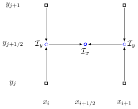
Figure 2: Illustration of the Hermite interpolation procedure in 2-D. The Hermite interpolation procedure along $x$ and $y$ are denoted respectively by $\mathcal{I}_{x}$ and $\mathcal{I}_{y}$. The primal nodes are represented by black squares while the cell center is represented by the blue circle.

To do so, we use tensor products of 1-D Hermite interpolants, as illustrated in Fig. 2. At the edge located at $x_{i}$ and for $k=0,\dots,m$, we compute the 1-D Hermite interpolant $p_{y,i}^{k}(y)$ for the $k^{\text{th}}$ $x$-derivative of $f$ that satisfies

$$\frac{\partial^{\ell}p_{y,i}^{k}(y_{j})}{\partial^{\ell}y}=\frac{\partial^{\ell}\partial^{k}f(x_{i},y_{j})}{\partial^{\ell}y\,\partial^{k}x},\quad\frac{\partial^{\ell}p_{y,i}^{k}(y_{j+1})}{\partial^{\ell}y}=\frac{\partial^{\ell}\partial^{k}f(x_{i},y_{j+1})}{\partial^{\ell}y\,\partial^{k}x},\quad\ell=0,\dots,m.$$

This gives us 1-D Hermite interpolants for the variable $f$ and its first $m$ $x$-derivatives along the edge connecting $(x_{i},y_{j})$ and $(x_{i},y_{j+1})$. A similar procedure is used to seek the 1-D Hermite interpolants $p_{y,i+1}^{k}(y)$ associated with the edge connecting $(x_{i+1},y_{j})$ and $(x_{i+1},y_{j+1})$. This step is represented by $\mathcal{I}_{y}$ in Fig. 2.

At the edge centers, we compute all the $y$-derivatives of the 1-D Hermite interpolants

$$\frac{\partial^{\ell}p_{y,i}^{k}(y_{j+1/2})}{\partial^{\ell}y},\quad\frac{\partial^{\ell}p_{y,i+1}^{k}(y_{j+1/2})}{\partial^{\ell}y},\quad k=0,\dots,m,\quad\ell=0,\dots,2\,m+1.$$

This is represented by the dashed blue circle in Fig. 2.

For $\ell=0,\dots,2\,m+1$, we then compute the 1-D Hermite interpolant $p_{x}^{\ell}(x)$ that satisfies

$$\frac{\partial^{k}p_{x}^{\ell}(x_{i})}{\partial^{k}x}=\frac{\partial^{k}\partial^{\ell}p_{y,i}^{k}(y_{j+1/2})}{\partial^{k}x\,\partial^{\ell}y},\quad\frac{\partial^{k}p_{x}^{\ell}(x_{i+1})}{\partial^{k}x}=\frac{\partial^{k}\partial^{\ell}p_{y,i+1}^{k}(y_{j+1/2})}{\partial^{k}x\,\partial^{\ell}y},\quad k=0,\dots,m.$$

Here $p_{x}^{\ell}(x)$ approximates the $\ell^{\text{th}}$ $y$-derivative of $f$. This is represented by $\mathcal{I}_{x}$ in Fig. 2.

To complete the Hermite interpolation, we approximate the variable and all its derivatives at the cell center

$$\frac{\partial^{k+\ell}f(x_{i+1/2},y_{j+1/2})}{\partial^{k}x\,\partial^{\ell}y}\approx\frac{\partial^{k}p_{x}^{\ell}(x_{i+1/2})}{\partial^{k}x},\quad k,\ell=0,\dots,2\,m+1,$$

and construct the 2-D Hermite interpolant

$$p_{i+1/2,j+1/2}^{f}(x,y)=\sum_{k=0}^{2\,m+1}\sum_{\ell=0}^{2\,m+1}\frac{\partial^{k}p_{x}^{\ell}(x_{i+1/2})}{\partial^{k}x}\frac{\Delta x^{k}\,\Delta y^{\ell}}{k!\,\ell!}\bigg{(}\frac{x-x_{i+1/2}}{\Delta x}\bigg{)}^{k}\bigg{(}\frac{y-y_{j+1/2}}{\Delta y}\bigg{)}^{\ell}.$$

Performing the 2-D Hermite interpolation for each cell and for each electromagnetic field at time $t_{0}$ gives us

$$H_{x}(x,y,t)|_{t=0}\approx \,\,p_{i+1/2,j+1/2}^{H_{x}}(x,y)=\sum_{k=0}^{2\,m+1}\sum_{\ell=0}^{2\,m+1}c_{k,\ell}^{H_{x}}(t)|_{t=0}\bigg{(}\frac{x-x_{i+1/2}}{\Delta x}\bigg{)}^{k}\bigg{(}\frac{y-y_{j+1/2}}{\Delta y}\bigg{)}^{\ell},$$

$$H_{y}(x,y,t)|_{t=0}\approx \,\,p_{i+1/2,j+1/2}^{H_{y}}(x,y)=\sum_{k=0}^{2\,m+1}\sum_{\ell=0}^{2\,m+1}c_{k,\ell}^{H_{y}}(t)|_{t=0}\bigg{(}\frac{x-x_{i+1/2}}{\Delta x}\bigg{)}^{k}\bigg{(}\frac{y-y_{j+1/2}}{\Delta y}\bigg{)}^{\ell},$$

$$E_{z}(x,y,t)|_{t=0}\approx \,\,p_{i+1/2,j+1/2}^{E_{z}}(x,y)=\sum_{k=0}^{2\,m+1}\sum_{\ell=0}^{2\,m+1}c_{k,\ell}^{E_{z}}(t)|_{t=0}\bigg{(}\frac{x-x_{i+1/2}}{\Delta x}\bigg{)}^{k}\bigg{(}\frac{y-y_{j+1/2}}{\Delta y}\bigg{)}^{\ell}.$$

Here $c_{k,\ell}^{H_{x}}$, $c_{k,\ell}^{H_{y}}$ and $c_{k,\ell}^{E_{z}}$ are time-dependent coefficients.

3.2 Recursion Relation

Let us now seek the Hermite-Taylor polynomials approximating the electromagnetic fields. Expanding in time the coefficients $c_{k,\ell}^{H_{x}}$, $c_{k,\ell}^{H_{y}}$ and $c_{k,\ell}^{E_{z}}$ leads to approximations of the form

$$p_{i+1/2,j+1/2}^{f}(x,y,t)=\sum_{k=0}^{2\,m+1}\sum_{\ell=0}^{2\,m+1}\sum_{s=0}^{q}c_{k,\ell,s}^{f}\bigg{(}\frac{x-x_{i+1/2}}{\Delta x}\bigg{)}^{k}\,\bigg{(}\frac{y-y_{j+1/2}}{\Delta y}\bigg{)}^{\ell}\,\bigg{(}\frac{t-t_{0}}{\Delta t}\bigg{)}^{q}.$$

Here $q$ is the degree of the Taylor polynomial.

For sufficiently smooth electromagnetic fields, we have from Maxwell’s equations (5)

$$\frac{\partial^{k+\ell+s+1}H_{x}}{\partial^{k}x\,\partial^{\ell}y\,\partial^{s+1}t}= \,\,-\frac{1}{\mu}\frac{\partial^{k+\ell+s+1}E_{z}}{\partial^{k}x\,\partial^{\ell+1}y\,\partial^{s}t},$$ (6)

$$\frac{\partial^{k+\ell+s+1}H_{y}}{\partial^{k}x\,\partial^{\ell}y\,\partial^{s+1}t}= \,\,\frac{1}{\mu}\frac{\partial^{k+\ell+s+1}E_{z}}{\partial^{k+1}x\,\partial^{\ell}y\,\partial^{s}t},$$

$$\frac{\partial^{k+\ell+s+1}E_{z}}{\partial^{k}x\,\partial^{\ell}y\,\partial^{s+1}t}= \,\,\frac{1}{\epsilon}\bigg{(}\frac{\partial^{k+\ell+s+1}H_{y}}{\partial^{k+1}x\,\partial^{\ell}y\,\partial^{s}t}-\frac{\partial^{k+\ell+s+1}H_{x}}{\partial^{k}x\,\partial^{\ell+1}y\,\partial^{s}t}\bigg{)}.$$

We then enforce the Hermite-Taylor polynomials approximating the electromagnetic fields to satisfy the system (6) at the cell center. This gives us the following recursion relations on the coefficients

$$c_{k,\ell,s}^{H_{x}}= \,\,-\frac{(\ell+1)\,\Delta t}{\mu\,s\Delta y}c^{E_{z}}_{k,\ell+1,s-1},$$ (7)

$$c_{k,\ell,s}^{H_{y}}= \,\,\frac{(k+1)\,\Delta t}{\mu\,s\Delta x}c^{E_{z}}_{k+1,\ell,s-1}$$

$$c_{k,\ell,s}^{E_{z}}= \,\,\frac{\Delta t}{\epsilon\,s}\bigg{(}\frac{(k+1)}{\Delta x}c^{H_{y}}_{k+1,\ell,s-1}-\frac{(\ell+1)}{\Delta y}c^{H_{x}}_{k,\ell+1,s-1}\bigg{)},$$

for $k,\ell=0,\dots,2\,m+1$ and $s=1,\dots,q$.

From the Hermite interpolants approximating the electromagnetic fields at $t_{0}$, we know $c_{k,\ell,0}^{H_{x}}$, $c_{k,\ell,0}^{H_{y}}$ and $c_{k,\ell,0}^{E_{z}}$ for all $k$ and $\ell$. Using the recursion relations (7), we can easily compute the remaining coefficients for $s>0$ and therefore compute the Hermite-Taylor polynomials.

3.3 Time Evolution

To evolve the data on the dual mesh at time $t_{1/2}$, we directly evaluate

$$\partial_{x}^{k}\,\partial_{y}^{\ell}p_{i+1/2,j+1/2}^{f}(x_{i+1/2},y_{j+1/2},t_{1/2}),\quad k,\ell=0,\dots,m,$$

for $f$ being $H_{x}$, $H_{y}$ and $E_{z}$.

To update the data on the primal mesh at time $t_{1}$ and therefore to complete the time step, we repeat a similar procedure for each cell $[x_{i-1/2},x_{i+1/2}]\times[y_{j-1/2},y_{j+1/2}]$ of the dual mesh and update the data on the primal mesh at $(x_{i},y_{j})$. Afterward, the whole procedure is repeated until the final time is reached.

For linear hyperbolic problems with constant coefficients, the Taylor expansion in time of the coefficients of Hermite interpolants is done exactly for $q=\nu\,(2\,m+1)$ in $\mathbb{R}^{\nu}$.

The enforcement of boundary conditions is challenging for the Hermite-Taylor method since all values of the electromagnetic fields and their derivatives through order $m$ in normal and tangential directions must also be known on the boundary, which is not the case in general. For an embedded boundary, the boundary can be located between the nodes of the mesh which further complicates the enforcement of boundary conditions. The imposition of interface conditions shares the same issue with the additional difficulty that the electromagnetic fields could be discontinuous at the interface. In the next section, we present a new avenue to handle embedded boundary and interface conditions based on the correction function method.

4 Correction Function Method

The correction function method seeks a polynomial approximating each electromagnetic field component in the vicinity of the nodes where the Hermite-Taylor method cannot be directly applied. We refer to such a node as a CF node. The node where the numerical solution can be updated using the Hermite-Taylor method is referred to as a Hermite node.

The correction function method relies on the minimization of a functional describing the electromagnetic fields in the vicinity of a CF node. The approximations of the electromagnetic fields are sought in a polynomial space and a careful definition of the space-time domain of the polynomials approximating the electromagnetic fields is required for accuracy.

In this section, we describe in detail the correction function method in 1-D for embedded boundary and interface problems. We then extend the method to the two-dimensional case.

4.1 Embedded Boundary in One Dimension

Let us consider the following 1-D simplification of Maxwell’s equations

$$\mu\,\partial_{t}H+\partial_{x}E= \,\,0,$$ (8)

$$\epsilon\,\partial_{t}E+\partial_{x}H= \,\,0,$$

in the domain $\Omega=[x_{\ell},x_{r}]$ and the time interval $[t_{0},t_{f}]$. Here $\mu$ and $\epsilon$ are constant. We enforce the boundary conditions

$$E(x_{\ell},t)=g_{\ell}(t)\qquad\mbox{and}\qquad E(x_{r},t)=g_{r}(t).$$

We consider the physical domain $\Omega$ to be embedded in a computational domain $\Omega_{c}=[x_{0},x_{N}]$. We then have two CF nodes, one for the left boundary and one for the right boundary. For simplicity, we assume that both CF nodes belong to the primal mesh.

For the $i^{\text{th}}$ CF node at time $t_{n}$, we define a functional

$$J_{i}^{n}=\mathcal{G}_{i}^{n}+\mathcal{B}_{i}^{n}+\mathcal{H}_{i}^{n}.$$ (9)

The first part $\mathcal{G}_{i}^{n}$ ensures that the governing equations are approximately fulfilled. The second part $\mathcal{B}_{i}^{n}$ weakly enforces the boundary conditions. The third part $\mathcal{H}_{i}^{n}$ weakly enforces the correction functions to match the Hermite solution.

Each part of the functional $J_{i}^{n}$ is computed over different domains. The electromagnetic fields are required to approximately satisfy Maxwell’s equations in the local patch of $J_{i}^{n}$. The space-time domain of the governing equations functional $\mathcal{G}_{i}^{n}$ then encloses the $i^{\text{th}}$ CF node, the domains of the boundary functional $\mathcal{B}_{i}^{n}$ and the Hermite functional $\mathcal{H}_{i}^{n}$. The domain of $\mathcal{B}_{i}^{n}$ encloses the part of the boundary close to the $i^{\text{th}}$ CF node. Finally, the domain of $\mathcal{H}_{i}^{n}$ encloses the space-time domains of the closest primal Hermite and dual Hermite nodes to the $i^{\text{th}}$ CF node.

As an example, let us consider that the left boundary is located at $x_{\ell}$ between the dual node $x_{1/2}$ and the primal node $x_{1}$. In this situation, we use the correction function method to update the numerical solution of the electromagnetic fields and their $m$ first derivatives located at the primal CF node $x_{1}$ at a given time $t_{n}$.

The governing equations functional $\mathcal{G}_{0}^{n}$ contains the residual of Maxwell’s equations and is integrated over the space-time domain $S_{0}\times[t_{n-1},t_{n}]$. Here the space interval is $S_{0}=[x_{\ell},x_{5/2}]$. The governing equations functional is then given by

$$\mathcal{G}_{0}^{n}(H^{n}_{h,0},E^{n}_{h,0})=\frac{\ell_{0}}{2}\,\int\limits_{t_{n-1}}^{t_{n}}\int\limits_{S_{0}}(\mu\,\partial_{t}H^{n}_{h,0}+\partial_{x}E^{n}_{h,0})^{2}+Z^{2}(\epsilon\,\partial_{t}E^{n}_{h,0}+\partial_{x}H^{n}_{h,0})^{2}\,\mathrm{d}x\,\mathrm{d}t.$$

Here $Z=\sqrt{\mu/\epsilon}$ is the impedance and $\ell_{0}=x_{5/2}-x_{\ell}$ is the characteristic length of the local patch, and $H^{n}_{h,0}$ and $E^{n}_{h,0}$ are the polynomials approximating the electromagnetic fields in the local patch that we seek. $H^{n}_{h,0}$ and $E^{n}_{h,0}$ are referred to as the correction functions. The integration domain of $\mathcal{G}^{n}_{0}$ is illustrated in Fig. 3.

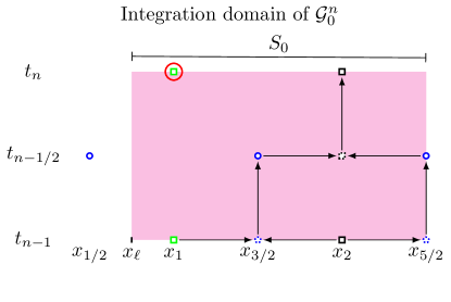
Figure 3: Illustration of the domain of integration $S_{0}\times[t_{n-1},t_{n}]$ of $\mathcal{G}_{0}^{n}$. The primal CF and Hermite nodes are respectively represented by green squares and black squares while the dual Hermite nodes are represented by blue circles. The CFM seeks the information located at $(x_{1},t_{n})$ which is enclosed by the red circle. The space-time local patch $S_{0}\times[t_{n-1},t_{n}]$ is denoted by a magenta box.

The boundary functional $\mathcal{B}_{0}^{n}$ contains the residual of the boundary condition at $x_{\ell}$ and is integrated over the time interval $[t_{n-1},t_{n}]$. We then have

$$\mathcal{B}_{0}^{n}(E^{n}_{h,0})=\frac{1}{2}\,\int\limits_{t_{n-1}}^{t_{n}}(E^{n}_{h,0}(x_{\ell},t)-g_{\ell}(t))^{2}\,\mathrm{d}t.$$

The integration domain of $\mathcal{B}_{0}^{n}$ is illustrated in Fig. 4.

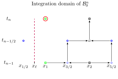
Figure 4: Illustration of the domain of integration $[t_{n-1},t_{n}]$ at $x_{\ell}$ of $\mathcal{B}_{0}^{n}$. The primal CF and Hermite nodes are respectively represented by green squares and black squares while the dual Hermite nodes are represented by blue circles. The CFM seeks the information located at $(x_{1},t_{n})$ which is enclosed by the red circle. The intersection between the boundary and the local patch, that is the line connecting $(x_{\ell},t_{n-1})$ to $(x_{\ell},t_{n})$, is denoted by a dashed purple line.

The Hermite functional

$$\mathcal{H}_{0}^{n}=\mathcal{H}_{p,0}^{n}+\mathcal{H}_{d,0}^{n},$$

weakly enforces the correction function to match the Hermite solution. The first part $\mathcal{H}_{p,0}^{n}$ weakly enforces the correction function to match the Hermite-Taylor polynomial associated with the primal Hermite node $x_{2}$ in the space-time domain $S_{0,p}^{\mathcal{H}}\times[t_{n-1/2},t_{n}]$. Here the space interval $S_{0,p}^{\mathcal{H}}=[x_{3/2},x_{5/2}]$. We obtain

$$\mathcal{H}_{p,0}^{n}(H^{n}_{h,0},E^{n}_{h,0})=\frac{1}{2}\frac{c_{H}}{\Delta x}\int\limits_{t_{n-\frac{1}{2}}}^{t_{n}}\int\limits_{S_{0,p}^{\mathcal{H}}}Z^{2}(H^{n}_{h,0}-H^{*})^{2}+(E^{n}_{h,0}-E^{*})^{2}\,\mathrm{d}x\,\mathrm{d}t.$$

Here $c_{H}>0$ is a given penalization parameter, and $H^{*}$ and $E^{*}$ are Hermite-Taylor polynomials. The second term $\mathcal{H}_{d,0}^{n}$ weakly enforces the Hermite-Taylor polynomial associated with the dual Hermite node $x_{3/2}$ in the space-time domain $S_{0,d}^{\mathcal{H}}\times[t_{n-1},t_{n-1/2}]$. Here the space interval is $S_{0,d}^{\mathcal{H}}=[x_{1},x_{2}]$. We then have

$$\mathcal{H}_{d,0}^{n}(H^{n}_{h,0},E^{n}_{h,0})=\frac{1}{2}\frac{c_{H}}{\Delta x}\int\limits_{t_{n-1}}^{t_{n-\frac{1}{2}}}\int\limits_{S_{0,d}^{\mathcal{H}}}Z^{2}(H^{n}_{h,0}-H^{*})^{2}+(E^{n}_{h,0}-E^{*})^{2}\,\mathrm{d}x\,\mathrm{d}t.$$

The integration domain of $\mathcal{H}_{0}^{n}$ is illustrated in Fig. 5.

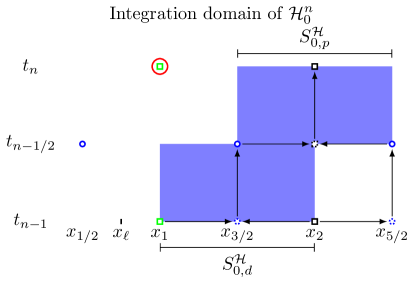
Figure 5: Illustration of the domains of integration $S_{0,p}^{\mathcal{H}}\times[t_{n-1/2},t_{n}]$ and $S_{0,d}^{\mathcal{H}}\times[t_{n-1},t_{n-1/2}]$ of $\mathcal{H}_{0}^{n}$. The primal CF and Hermite nodes are respectively represented by green squares and black squares while the dual Hermite nodes are represented by blue circles. The CFM seeks the information located at $(x_{1},t_{n})$ which is enclosed by the red circle. The domains $S_{0,p}^{\mathcal{H}}\times[t_{n-1/2},t_{n}]$ and $S_{0,d}^{\mathcal{H}}\times[t_{n-1},t_{n-1/2}]$, where we enforce the correction functions to match the Hermite-Taylor polynomials, are denoted by blue boxes.

The procedure described above can be easily adapted to weakly enforce the boundary condition at $x_{r}$.

4.1.1 The Linear System of Equations that Solves the Optimization Problem

For each CF node, we solve the following minimization problem

$$\text{Find }(H^{n}_{h,i},E^{n}_{h,i})\in V\times V\text{ such that }$$ (10)

$$\qquad(H^{n}_{h,i},E^{n}_{h,i})=\underset{v,w\in V}{\arg\min}\,J_{i}^{n}(v,w).$$

Here $V=\mathbb{Q}^{k}\big{(}S_{i}\times[t_{n-1},t_{n}]\big{)}$ is the space of tensor-product polynomials of degree at most $k$ in each variable, $n=1,\dots,N_{t}$ and $i=0,1$ in our 1-D example. We use space-time Legendre polynomials as basis functions of $V$.

To solve the minimization problem (10), we compute the gradient of $J_{i}^{n}$ with respect to the coefficients of the polynomials $H^{n}_{h,i}$ and $E^{n}_{h,i}$ and use that it vanishes at a minimum. We then obtain the linear system of equations

$$M_{i}^{n}\,\mathbold{c}_{i}^{n}=\mathbold{b}_{i}^{n}.$$

Here $M_{i}^{n}$ is a square matrix of dimension $2\,(k+1)^{2}$ and $\mathbold{c}_{i}^{n}$ is a vector containing the polynomials coefficients. Note that the dimension of the matrices $M_{i}^{n}$ is independent of the mesh size.

Since the boundary is invariant in time, we have $M_{i}=M_{i}^{n}$ for all $n$ and therefore obtain one matrix per CF node. The matrices, $M_{i}$, their scaling and their LU factorization are all precomputed. For each time step, we then have to compute the right-hand side $\mathbold{b}_{i}^{n}$, perform forward and backward substitutions to find $\mathbold{c}_{i}^{n}$, and update the numerical solution of the electromagnetic fields and their first $m$ derivatives at the $i^{\text{th}}$ CF node using $H^{n}_{h,i}$ and $E^{n}_{h,i}$. This can be done independently for each $i$.

Remark 1

A similar procedure can be done to update the data located at dual CF nodes. However, the first time step is different because we do not know the electromagnetic fields and their first $m$ space derivatives at time $t_{-1/2}$. We therefore use the Hermite-Taylor correction function method proposed in LawAppelo2022 for the dual CF nodes at the first time step.

Assume that there are CF nodes on the primal and dual meshes. Given the numerical solution on the primal mesh at $t_{n-1}$ and on the dual mesh at $t_{n-3/2}$, the algorithm to evolve the numerical solution at $t_{n}$ is

• Update the numerical solution on the dual Hermite node at $t_{n-1/2}$ using the Hermite-Taylor method and store the Hermite-Taylor polynomials needed for the CFM;

• Update the numerical solution on the dual CF nodes at $t_{n-1/2}$ using the CFM by computing $\mathbold{b}_{i}^{n-1/2}$ and solving for $\mathbold{c}_{i}^{n-1/2}$;

• Update the numerical solution on the primal Hermite node at $t_{n}$ using the Hermite-Taylor method and store the Hermite-Taylor polynomials needed for the CFM;

• Update the numerical solution on the primal CF nodes at $t_{n}$ using the CFM by computing $\mathbold{b}_{i}^{n}$ and solving for $\mathbold{c}_{i}^{n}$.

4.2 Interface in One Dimension

Let us now consider 1-D interface problems. In addition to Maxwell’s equations (8), we consider the interface conditions

$$\llbracket H\rrbracket=0\qquad\mbox{and}\qquad\llbracket E\rrbracket=0,$$

on the interface $\Gamma$ located at $x_{\Gamma}$. We define the subdomains $\Omega^{+}=[x_{\ell},x_{\Gamma}]$ and $\Omega^{-}=[x_{\Gamma},x_{r}]$. The physical parameters $\mu$ and $\epsilon$ are assumed to be piecewise constant.

In this situation, we seek approximations of the electromagnetic fields in each subdomain for a given CF node. For each CF node, we then compute $H^{+,n}_{h}$ and $E^{+,n}_{h}$ approximating the electromagnetic fields in $\Omega^{+}$, and $H^{-,n}_{h}$ and $E^{-,n}_{h}$ approximating the electromagnetic fields in $\Omega^{-}$.

For the $i^{\text{th}}$ CF node at time $t_{n}$, we define a functional

$$J_{i}^{n}=\mathcal{G}_{i}^{+,n}+\mathcal{G}_{i}^{-,n}+\mathcal{I}_{i}^{n}+\mathcal{H}_{i}^{+,n}+\mathcal{H}_{i}^{-,n}.$$ (11)

The governing equations functionals $\mathcal{G}_{i}^{+,n}$ and $\mathcal{G}_{i}^{-,n}$ ensure that Maxwell’s equations in respectively $\Omega^{+}$ and $\Omega^{-}$ are approximately fulfilled. The interface functional $\mathcal{I}_{i}^{n}$ weakly enforces the interface conditions. The Hermite functional $\mathcal{H}_{i}^{+,n}$ weakly enforces the correction functions $H^{+,n}_{h,i}$ and $E^{+,n}_{h,i}$ to match the Hermite solution in $\Omega^{+}$ while $\mathcal{H}_{i}^{-,n}$ weakly enforces the correction functions $H^{-,n}_{h,i}$ and $E^{-,n}_{h,i}$ to match the Hermite solution in $\Omega^{-}$.

As for embedded boundary problems, each part of the functional $J_{i}^{n}$ is computed in different domains. The domains of $\mathcal{G}_{i}^{+,n}$ and $\mathcal{G}_{i}^{-,n}$ enclose the $i^{\text{th}}$ CF node, the domains of the interface functional and the Hermite functionals. This then defines the local patch of the $i^{\text{th}}$ CF node. The interface functional $\mathcal{I}_{i}^{n}$ encloses the part of the interface close to the $i^{\text{th}}$ CF node. The Hermite functional $\mathcal{H}_{i}^{+,n}$ encloses the space-time domains of the closest primal Hermite and dual Hermite nodes in $\Omega^{+}$ to the $i^{\text{th}}$ CF node. Finally, the Hermite functional $\mathcal{H}_{i}^{-,n}$ encloses the domains of the closest primal Hermite and dual Hermite nodes in $\Omega^{-}$ to the $i^{\text{th}}$ CF node.

As an example, we assume an interface $\Gamma$ located at $x_{\Gamma}$ between the dual node $x_{19/2}$ and the primal node $x_{10}$. In this situation, there are two CF nodes, one primal CF node located at $x_{10}$ and one dual CF node located at $x_{19/2}$. We focus now on the primal CF node.

The governing equations functional $\mathcal{G}_{0}^{+,n}$ contains the residual of Maxwell’s equations with the parameters from $\Omega^{+}$ and is integrated over the domain $S_{0}\times[t_{n-1},t_{n}]$. Here the space interval $S_{0}=[x_{8},x_{23/2}]$. We have

$$\mathcal{G}_{0}^{+,n}(H^{+,n}_{h,0},E^{+,n}_{h,0})= \,\,\frac{\ell_{0}}{2}\,\int\limits_{t_{n-1}}^{t_{n}}\int\limits_{S_{0}}(\mu^{+}\,\partial_{t}H^{+,n}_{h,0}+\partial_{x}E^{+,n}_{h,0})^{2}$$

$$+ \,\,(Z^{+})^{2}(\epsilon^{+}\,\partial_{t}E^{+,n}_{h,0}+\partial_{x}H^{+,n}_{h,0})^{2}\,\mathrm{d}x\,\mathrm{d}t.$$

Here the characteristic length of the local patch is $\ell_{0}=x_{23/2}-x_{8}$. The governing equations functional $\mathcal{G}_{0}^{-,n}$ is defined on the same domain as the functional $\mathcal{G}_{0}^{+,n}$ but contains the residual of Maxwell’s equations with the parameters from $\Omega^{-}$. We then have

$$\mathcal{G}_{0}^{-,n}(H^{-,n}_{h,0},E^{-,n}_{h,0})= \,\,\frac{\ell_{0}}{2}\,\int\limits_{t_{n-1}}^{t_{n}}\int\limits_{S_{0}}(\mu^{-}\,\partial_{t}H^{-,n}_{h,0}+\partial_{x}E^{-,n}_{h,0})^{2}$$

$$+ \,\,(Z^{-})^{2}(\epsilon^{-}\,\partial_{t}E^{-,n}_{h,0}+\partial_{x}H^{-,n}_{h,0})^{2}\,\mathrm{d}x\,\mathrm{d}t.$$

The domain of integration of the governing equations functionals $\mathcal{G}_{0}^{+,n}$ and $\mathcal{G}_{0}^{-,n}$ is shown in Fig. 6.

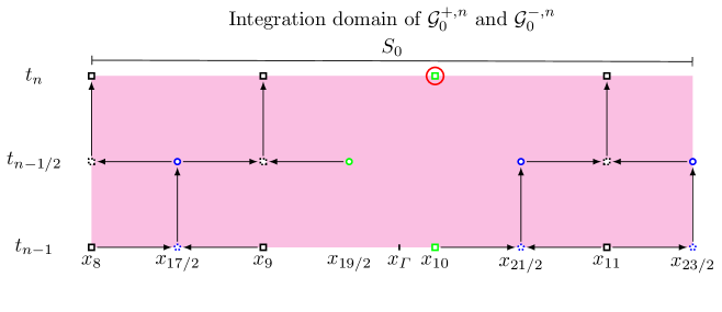
Figure 6: Illustration of the domain of integration $S_{0}\times[t_{n-1},t_{n}]$ of $\mathcal{G}_{0}^{+,n}$ and $\mathcal{G}_{0}^{-,n}$. The primal CF and Hermite nodes are respectively represented by green squares and black squares while the dual CF and Hermite nodes are represented by green circles and blue circles. The CFM seeks the information located at $(x_{10},t_{n})$ which is enclosed by the red circle. The space-time local patch $S_{0}\times[t_{n-1},t_{n}]$ is denoted by a magenta box.

The interface functional $\mathcal{I}_{0}^{n}$ contains the residual of the interface conditions, which in this case we take to be continuity for $E$ and $H$, and is integrated over the time interval $[t_{n-1},t_{n}]$. We then have

$$\mathcal{I}_{0}^{n}(H^{+,n}_{h,0},E^{+,n}_{h,0},H^{-,n}_{h,0},E^{-,n}_{h,0})=\frac{1}{2}\,\int\limits_{t_{n-1}}^{t_{n}}\bar{Z}^{2}\llbracket H^{n}_{h,0}(x_{\Gamma},t)\rrbracket^{2}+\llbracket E^{n}_{h,0}(x_{\Gamma},t)\rrbracket^{2}\,\mathrm{d}t.$$

Note that the interface functional couples the electromagnetic fields from the different subdomains at the interface. We can take $\bar{Z}=(Z^{+}+Z^{-})/2$ or the values from the left or right as convenient. The integration domain of $\mathcal{I}_{0}^{n}$ is illustrated in Fig. 7.

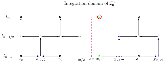
Figure 7: Illustration of the domain of integration $[t_{n-1},t_{n}]$ at $x_{\Gamma}$ of $\mathcal{I}_{0}^{n}$. The primal CF and Hermite nodes are respectively represented by green squares and black squares while the dual CF and Hermite nodes are represented by green circles and blue circles. The CFM seeks the information located at $(x_{10},t_{n})$ which is enclosed by the red circle. The intersection between the interface and the local patch, that is the line connecting $(x_{\Gamma},t_{n-1})$ to $(x_{\Gamma},t_{n})$, is denoted by a dashed purple line.

The Hermite functional $\mathcal{H}_{0}^{+,n}$ weakly enforces the correction functions $H^{+,n}_{h,0}$ and $E^{+,n}_{h,0}$ to match the Hermite solution in $\Omega^{+}$ over the domains $S_{p,0}^{\mathcal{H}^{+}}\times[t_{n-1/2},t_{n}]$ and $S_{d,0}^{\mathcal{H}^{+}}\times[t_{n-1},t_{n-1/2}]$. Here $S_{p,0}^{\mathcal{H}^{+}}=[x_{21/2},x_{23/2}]$ is the space interval of the primal Hermite node $x_{11}$ and $S_{d,0}^{\mathcal{H}^{+}}=[x_{10},x_{11}]$ is the space interval of the dual Hermite node $x_{21/2}$. We then have

$$\mathcal{H}_{0}^{+,n}=\mathcal{H}_{p,0}^{+,n}+\mathcal{H}_{d,0}^{+,n},$$

with

$$\mathcal{H}_{p,0}^{+,n}(H^{+,n}_{h,0},E^{+,n}_{h,0})= \,\,\frac{1}{2}\frac{c_{H}}{\Delta x}\int\limits_{t_{n-\frac{1}{2}}}^{t_{n}}\int\limits_{S_{0,p}^{\mathcal{H}^{+}}}(Z^{+})^{2}(H^{+,n}_{h,0}-H^{*})^{2}+(E^{+,n}_{h,0}-E^{*})^{2}\,\mathrm{d}x\,\mathrm{d}t,$$

$$\mathcal{H}_{d,0}^{+,n}(H^{+,n}_{h,0},E^{+,n}_{h,0})= \,\,\frac{1}{2}\frac{c_{H}}{\Delta x}\int\limits_{t_{n-1}}^{t_{n-\frac{1}{2}}}\int\limits_{S_{0,d}^{\mathcal{H}^{+}}}(Z^{+})^{2}(H^{+,n}_{h,0}-H^{*})^{2}+(E^{+,n}_{h,0}-E^{*})^{2}\,\mathrm{d}x\,\mathrm{d}t.$$

Finally, the Hermite functional $\mathcal{H}_{0}^{-,n}$ weakly enforces the correction functions $H^{-,n}_{h,0}$ and $E^{-,n}_{h,0}$ to match the Hermite solution in $\Omega^{-}$ over the domains $S_{p,0}^{\mathcal{H}^{-}}\times[t_{n-1/2},t_{n}]$ and $S_{d,0}^{\mathcal{H}^{-}}\times[t_{n-1},t_{n-1/2}]$. Here the space intervals $S_{p,0}^{\mathcal{H}^{-}}=[x_{17/2},x_{19/2}]$ and $S_{d,0}^{\mathcal{H}^{-}}=[x_{8},x_{9}]$. We obtain

$$\mathcal{H}_{0}^{-,n}=\mathcal{H}_{p,0}^{-,n}+\mathcal{H}_{d,0}^{-,n},$$

with

$$\mathcal{H}_{p,0}^{-,n}(H^{-,n}_{h,0},E^{-,n}_{h,0})= \,\,\frac{1}{2}\frac{c_{H}}{\Delta x}\int\limits_{t_{n-\frac{1}{2}}}^{t_{n}}\int\limits_{S_{0,p}^{\mathcal{H}^{-}}}(Z^{-})^{2}(H^{-,n}_{h,0}-H^{*})^{2}+(E^{-,n}_{h,0}-E^{*})^{2}\,\mathrm{d}x\,\mathrm{d}t,$$

$$\mathcal{H}_{d,0}^{-,n}(H^{-,n}_{h,0},E^{-,n}_{h,0})= \,\,\frac{1}{2}\frac{c_{H}}{\Delta x}\int\limits_{t_{n-1}}^{t_{n-\frac{1}{2}}}\int\limits_{S_{0,d}^{\mathcal{H}^{-}}}(Z^{-})^{2}(H^{-,n}_{h,0}-H^{*})^{2}+(E^{-,n}_{h,0}-E^{*})^{2}\,\mathrm{d}x\,\mathrm{d}t.$$

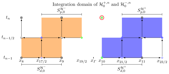
Figure 8: Illustration of the domains of integration $S_{0,p}^{\mathcal{H}^{+}}\times[t_{n-1/2},t_{n}]$, $S_{0,d}^{\mathcal{H}^{+}}\times[t_{n-1},t_{n-1/2}]$, $S_{0,p}^{\mathcal{H}^{-}}\times[t_{n-1/2},t_{n}]$ and $S_{0,d}^{\mathcal{H}^{-}}\times[t_{n-1},t_{n-1/2}]$ of $\mathcal{H}_{0}^{+,n}$ and $\mathcal{H}_{0}^{-,n}$. The primal CF and Hermite nodes are respectively represented by green squares and black squares while the dual CF and Hermite nodes are represented by green circles and blue circles. The CFM seeks the information located at $(x_{10},t_{n})$ which is enclosed by the red circle. The domains of $\mathcal{H}_{0}^{+,n}$ and $\mathcal{H}_{0}^{-,n}$, where we enforce the correction functions to match the Hermite-Taylor polynomials, are denoted respectively by blue boxes and orange boxes.

A similar procedure is used to define the functional $J^{n-1/2}$ associated with the dual CF node $x_{19/2}$.

4.2.1 The Linear System of Equations that Solves the Optimization Problem

For each CF node, we solve the following minimization problem

$$\text{Find }(H^{+,n}_{h,i},E^{+,n}_{h,i},H^{-,n}_{h,i},E^{-,n}_{h,i})\in V\times V\times V\times V\text{ such that }$$ (12)

$$\qquad(H^{+,n}_{h,i},E^{+,n}_{h,i},H^{-,n}_{h,i},E^{-,n}_{h,i})=\underset{v^{+},w^{+},v^{-},w^{-}\in V}{\arg\min}\,J_{i}^{n}(v^{+},w^{+},v^{-},w^{-}).$$

We solve the minimization problem (12) using a procedure similar to that of the embedded boundary case. We therefore have the same properties as before, except that the dimension of the resulting linear system becomes $4\,(k+1)^{2}$. The algorithm of the Hermite-Taylor correction function method to evolve the numerical solution remains the same as for the embedded boundary case.

4.3 Multi-Dimensional Case

In this subsection, we extend the Hermite-Taylor correction function method to two and three dimensions for embedded boundary and interface problems.

4.3.1 Computation of the Local Patches

In the multi-dimensional case, the time component of the local patches remains the same for all CF nodes while their spatial components are adapted to the geometry of the boundary (or interface). The spatial component $S_{i}$ of the $i^{\text{th}}$ CF node local patch needs to satisfy the following three constraints:

• The $i^{\text{th}}$ CF node must be inside;

• The part of the boundary (or interface) closest to the $i^{\text{th}}$ CF node must be included in the local patch;

• The cells of the Hermite nodes closest to the $i^{\text{th}}$ CF node must be included in the local patch.

Focusing in detail on two space dimensions for simplicity, we define the dimension of the space component $S_{i}$ to be $\beta\,h\times\beta\,h$. Here $h=\Delta x=\Delta y$ is the mesh size and $\beta$ is a given positive constant that depends on the geometry of the boundary (or interface). Since the update of the numerical solution with the Hermite-Taylor method for one half time step uses a five-node stencil, we therefore have one layer of CF nodes inside the domain along the boundary. As for the interface case, we have one layer of CF nodes inside each subdomain along the interface. The space component $S_{i}$ of the local patch is then centered at the $i^{\text{th}}$ CF node to enclose the closest part of the boundary (or interface) to the CF node as well as its closest Hermite cells.

Once the space-time domains of the local patches are computed, it is easy to identify the primal and dual Hermite nodes located inside the local patches and compute the space-time regions for the Hermite functionals. Fig. 9 and Fig. 10 illustrate examples of a local patch with $\beta=5$ for respectively an embedded boundary problem and an interface problem.

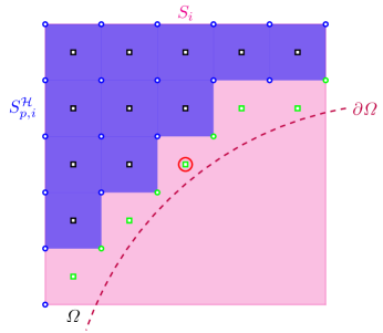
Figure 9: Illustration of a 2-D local patch for an embedded boundary problem. The primal CF and Hermite nodes are respectively represented by green squares and black squares while the dual CF and Hermite nodes are represented by green circles and blue circles. The CFM seeks the information located at the primal CF node enclosed by the red circle. The spatial domain $S_{i}$ of the local patch is denoted by a magenta box. The boundary $\partial\Omega$ is denoted by a dashed purple line. The domains $S_{p,i}^{\mathcal{H}}$ and $S_{d,i}^{\mathcal{H}}$ where we enforce the correction functions to match the Hermite-Taylor polynomials are denoted by blue boxes. The left plot is for the spatial components of the local patch over the time interval $[t_{n-1/2},t_{n}]$ while the right plot is for $[t_{n-1},t_{n-1/2}]$.

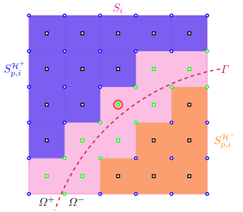
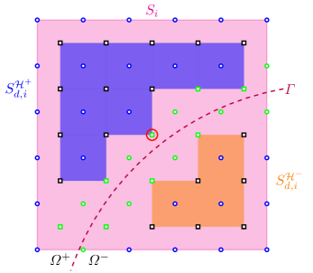
Figure 10: Illustration of a 2-D local patch for an interface problem. The primal CF and Hermite nodes are respectively represented by green squares and black squares while the dual CF and Hermite nodes are represented by green circles and blue circles. The CFM seeks the information located at the primal CF node enclosed by the red circle. The spatial domain $S_{i}$ of the local patch is denoted by a magenta box. The interface $\Gamma$ is denoted by a dashed purple line. The domains $S_{p,i}^{\mathcal{H}^{+}}$ and $S_{d,i}^{\mathcal{H}^{+}}$ where we enforce the correction functions to match the Hermite-Taylor polynomials in $\Omega^{+}$ are denoted by blue boxes. The domains $S_{p,i}^{\mathcal{H}^{-}}$ and $S_{d,i}^{\mathcal{H}^{-}}$ are denoted by orange boxes. The left plot is for the spatial components of the local patch over the time interval $[t_{n-1/2},t_{n}]$ while the right plot is for $[t_{n-1},t_{n-1/2}]$.

4.3.2 Definition of the Correction Function Functional

Let us first focus on the embedded boundary case. For simplicity, we consider that all the CF nodes belong to the primal mesh. The described procedure below can be easily adapted to define the functional for a dual CF node.

As in the one dimensional case, for each primal CF node, we define the functional (9) to seek the polynomials $\mathbold{H}_{h,i}^{n}$ and $\mathbold{E}_{h,i}^{n}$ approximating the electromagnetic fields in the local patch. The governing equations functional becomes

$$\mathcal{G}_{i}^{n}(\mathbold{H}^{n}_{h,i},\mathbold{E}^{n}_{h,i})= \,\,\frac{\ell_{i}}{2}\,\int\limits_{t_{n-1}}^{t_{n}}\int\limits_{S_{i}}(\mu\,\partial_{t}\mathbold{H}^{n}_{h,i}+\nabla\times\mathbold{E}^{n}_{h,i})\cdot(\mu\,\partial_{t}\mathbold{H}^{n}_{h,i}+\nabla\times\mathbold{E}^{n}_{h,i})$$

$$+ \,\,Z^{2}(\epsilon\,\partial_{t}\mathbold{E}^{n}_{h,i}-\nabla\times\mathbold{H}^{n}_{h,i})\cdot(\epsilon\,\partial_{t}\mathbold{E}^{n}_{h,i}-\nabla\times\mathbold{H}^{n}_{h,i})$$

$$+ \,\,c^{2}(\nabla\cdot(\mu\,\mathbold{H}^{n}_{h,i}))^{2}+\frac{1}{\epsilon^{2}}(\nabla\cdot(\epsilon\,\mathbold{E}^{n}_{h,i}))^{2}\,\mathrm{d}\mathbold{x}\,\mathrm{d}t.$$

Here $c=1/\sqrt{\epsilon\mu}$ is the wave speed and the characteristic length of the local patch is $\ell_{i}=\beta\,h$. The second part of the functional $J_{i}^{n}$ that weakly enforces the boundary condition (3) becomes

$$\mathcal{B}_{i}^{n}(\mathbold{E}^{n}_{h,i})=\frac{1}{2}\,\int\limits_{t_{n-1}}^{t_{n}}\int\limits_{\partial\Omega\cap S_{i}}(\mathbold{n}\times\mathbold{E}^{n}_{h,i}-\mathbold{g})\cdot(\mathbold{n}\times\mathbold{E}^{n}_{h,i}-\mathbold{g})\,\mathrm{d}s\,\mathrm{d}t.$$

Finally, the two parts in the Hermite functional $\mathcal{H}_{i}^{n}$ become

$$\mathcal{H}_{p,i}^{n}(\mathbold{H}^{n}_{h,i},\mathbold{E}^{n}_{h,i})= \,\,\frac{1}{2}\frac{c_{H}}{h}\int\limits_{t_{n-\frac{1}{2}}}^{t_{n}}\int\limits_{S^{\mathcal{H}}_{p,i}}Z^{2}(\mathbold{H}^{n}_{h,i}-\mathbold{H}^{*})\cdot(\mathbold{H}^{n}_{h,i}-\mathbold{H}^{*})$$

$$+ \,\,(\mathbold{E}^{n}_{h,i}-\mathbold{E}^{*})\cdot(\mathbold{E}^{n}_{h,i}-\mathbold{E}^{*})\,\mathrm{d}\mathbold{x}\,\mathrm{d}t,$$

$$\mathcal{H}_{d,i}^{n}(\mathbold{H}^{n}_{h,i},\mathbold{E}^{n}_{h,i})= \,\,\frac{1}{2}\frac{c_{H}}{h}\int\limits_{t_{n-1}}^{t_{n-\frac{1}{2}}}\int\limits_{S^{\mathcal{H}}_{d,i}}Z^{2}(\mathbold{H}^{n}_{h,i}-\mathbold{H}^{*})\cdot(\mathbold{H}^{n}_{h,i}-\mathbold{H}^{*})$$

$$+ \,\,(\mathbold{E}^{n}_{h,i}-\mathbold{E}^{*})\cdot(\mathbold{E}^{n}_{h,i}-\mathbold{E}^{*})\,\mathrm{d}\mathbold{x}\,\mathrm{d}t.$$

As for the interface case, the functionals of the governing equations and the Hermite functionals in (11) are modified in the same way as the embedded boundary case. The interface functional that weakly enforces the interface conditions (4) becomes

$$\mathcal{I}_{i}^{n}(\mathbold{H}^{+,n}_{h,i},\mathbold{E}^{+,n}_{h,i},\mathbold{H}^{-,n}_{h,i},\mathbold{E}^{-,n}_{h,i})= \,\,\frac{1}{2}\,\int\limits_{t_{n-1}}^{t_{n}}\int\limits_{\Gamma\cap S_{i}}\left(\hat{\mathbold{n}}\times\llbracket\mathbold{E}^{n}_{h,i}\rrbracket\right)\cdot\left(\hat{\mathbold{n}}\times\llbracket\mathbold{E}^{n}_{h,i}\rrbracket\right)$$

$$+ \,\,\bar{Z}^{2}\left(\hat{\mathbold{n}}\times\llbracket\mathbold{H}^{n}_{h,i}\rrbracket\right)\cdot\left(\hat{\mathbold{n}}\times\llbracket\mathbold{H}^{n}_{h,i}\rrbracket\right)+\frac{1}{\bar{\epsilon}^{2}}(\hat{\mathbold{n}}\cdot\llbracket\epsilon\,\mathbold{E}^{n}_{h,i}\rrbracket)^{2}$$

$$+ \,\,\bar{c}^{2}(\hat{\mathbold{n}}\cdot\llbracket\mu\,\mathbold{H}^{n}_{h,i}\rrbracket)^{2}\,\mathrm{d}s\,\mathrm{d}t.$$

Here again the barred coefficients can be taken as averages or values from either side of the interface.

4.3.3 The Linear System of Equations that Solves the Optimization Problems

For each CF node and for each time step, we solve the following minimization problems

$$\text{Find }(\mathbold{H}^{n}_{h,i},\mathbold{E}^{n}_{h,i})\in V\times V\text{ such that }$$ (13)

$$\qquad(\mathbold{H}^{n}_{h,i},\mathbold{E}^{n}_{h,i})=\underset{\mathbold{v},\mathbold{w}\in V}{\arg\min}\,J_{i}^{n}(\mathbold{v},\mathbold{w}),$$

for the embedded boundary case and

$$\text{Find }(\mathbold{H}^{+,n}_{h,i},\mathbold{E}^{+,n}_{h,i},\mathbold{H}^{-,n}_{h,i},\mathbold{E}^{-,n}_{h,i})\in V\times V\times V\times V\text{ such that }$$ (14)

$$\qquad(\mathbold{H}^{+,n}_{h,i},\mathbold{E}^{+,n}_{h,i},\mathbold{H}^{-,n}_{h,i},\mathbold{E}^{-,n}_{h,i})=\underset{\mathbold{v}^{+},\mathbold{w}^{+},\mathbold{v}^{-},\mathbold{w}^{-}\in V}{\arg\min}\,J_{i}^{n}(\mathbold{v}^{+},\mathbold{w}^{+},\mathbold{v}^{-},\mathbold{w}^{-}),$$

for the interface case. Here, in general,

$$V=\{\mathbold{v}\in[\mathbb{Q}^{k}(S_{i}\times[t_{n-1},t_{n}])]^{3}\},$$

with the obvious reduction in dimensions if TM or TE modes are evolved.

We solve the minimization problems (13) and (14) using a procedure similar to that of the one-dimensional case. We therefore compute the matrices of the linear systems of equations, their scaling and LU factorizations as a pre-computation step. The dimension of the matrices is $3\,(k+1)^{3}$ for problems posed in two space dimensions and $6\,(k+1)^{4}$ in three space dimensions for the embedded boundary case. As for the interface case, the dimension of the matrices is $6\,(k+1)^{3}$ in two space dimensions and $12\,(k+1)^{4}$ in three space dimensions.

For each update of the numerical solution, we therefore need to compute the right-hand side of the linear systems of equations, solve for the polynomials coefficients and approximate the electromagnetic fields and the required space derivatives at the CF node using the correction functions. The algorithm of the Hermite-Taylor correction function method to evolve the numerical solution remains the same as the one-dimensional case.

The following propositions guarantee that the minimization problems (13) and (14) are well-posed.

Proposition 1

The minimization problem (13) has a unique global minimizer.

Proof

Since we are seeking the correction functions in the polynomial space $V$, we have

$$\mathbold{H}_{h,i}^{n}=\sum_{j=0}^{k+1}c_{i,j}^{H,n}\mathbold{\phi}_{j}\qquad\mbox{and}\qquad\mathbold{E}_{h,i}^{n}=\sum_{j=0}^{k+1}c_{i,j}^{E,n}\mathbold{\phi}_{j}.$$

Here $c_{i,j}^{H,n}$ and $c_{i,j}^{E,n}$ are scalars, and $\mathbold{\phi}_{j}$ are basis functions of the polynomial space $V$. The quadratic functional $J_{i}^{n}$ can therefore be written has

$$J_{i}^{n}(\mathbold{c}_{i}^{n})=r_{i}^{n}+(\mathbold{g}_{i}^{n})^{T}\mathbold{c}_{i}^{n}+\frac{1}{2}(\mathbold{c}_{i}^{n})^{T}M_{i}\mathbold{c}_{i}^{n}.$$ (15)

Here $\mathbold{c}_{i}^{n}$ is a vector containing the coefficients $c_{i,j}^{H,n}$ and $c_{i,j}^{E,n}$ for all $j$. Let us now verify that $M$ is a positive definite matrix to ensure that we have a global minimizer. Assuming $\mathbold{c}_{i}^{n}\neq 0$, we notice that

$$\frac{1}{2}(\mathbold{c}_{i}^{n})^{T}M_{i}\mathbold{c}_{i}^{n}= \,\,\underbrace{\mathcal{G}_{i}^{n}(\mathbold{H}^{n}_{h,i},\mathbold{E}^{n}_{h,i})}_{\geq 0}+\underbrace{\frac{1}{2}\,\int\limits_{t_{n-1}}^{t_{n}}\int\limits_{\partial\Omega\cap S_{i}}\left(\mathbold{n}\times\mathbold{E}^{n}_{h,i}\right)\cdot\left(\mathbold{n}\times\mathbold{E}^{n}_{h,i}\,\right)\mathrm{d}s\,\mathrm{d}t}_{\geq 0}$$

$$+ \,\,\underbrace{\frac{1}{2}\frac{c_{H}}{h}\int\limits_{t_{n-\frac{1}{2}}}^{t_{n}}\int\limits_{S^{\mathcal{H}}_{p,i}}Z^{2}\mathbold{H}^{n}_{h,i}\cdot\mathbold{H}^{n}_{h,i}+\mathbold{E}^{n}_{h,i}\cdot\mathbold{E}^{n}_{h,i}\,\mathrm{d}\mathbold{x}\,\mathrm{d}t}_{>0}$$

$$+ \,\,\underbrace{\frac{1}{2}\frac{c_{H}}{h}\int\limits_{t_{n-1}}^{t_{n-\frac{1}{2}}}\int\limits_{S^{\mathcal{H}}_{d,i}}Z^{2}\mathbold{H}^{n}_{h,i}\cdot\mathbold{H}^{n}_{h,i}+\mathbold{E}^{n}_{h,i}\cdot\mathbold{E}^{n}_{h,i}\,\mathrm{d}\mathbold{x}\,\mathrm{d}t}_{>0},$$

since only the zero polynomial can vanish uniformly on $S^{\mathcal{H}_{p,i}}\times(t_{n-1/2},t_{n})$ or $S^{\mathcal{H}_{d,i}}\times(t_{n-1},t_{n-1/2})$. The matrix $M_{i}$ is therefore positive definite and the minimization problem (13) has a global minimizer.

Proposition 2

The minimization problem (14) has a unique global minimizer.

Proof

The proof is similar to that of Proposition 1.

Remark 2

Let us assume that $k=2\,m$ and that polynomials approximating the correction functions have an accuracy of $\mathcal{O}(\ell_{i}^{k+1})$. Using

$$\mathbold{H}^{n}_{i}= \,\,\mathbold{H}+\mathcal{O}(\ell_{i}^{k+1}),$$

$$\mathbold{E}^{n}_{i}= \,\,\mathbold{E}+\mathcal{O}(\ell_{i}^{k+1}),$$

in the functional $J_{i}^{n}$ we obtain that all terms in the functional $J_{i}^{n}$ scale as $\mathcal{O}(\ell_{i}^{2\,k+5})$. Here $J_{i}^{n}$ is either given by (9) for an embedded boundary problem or (11) for an interface problem. We require that $c_{H}>0$ to have a well-posed minimization problem. We also require that $c_{H}<1$ so that the Hermite functionals are dominated by the Maxwell’s equations residuals and the boundary or interface conditions in $J_{i}^{n}$.

Remark 3

The correction function method should preserve the accuracy of the Hermite-Taylor method if $k=2\,m$. As for the stability, the correction function method impacts the stability properties of the numerical method used inside the domain as was remarked in LawNave2021 . The parameter $c_{H}$ must then be chosen small enough to obtain a stable Hermite-Taylor correction function method. However, $c_{H}$ cannot be taken arbitrary small to avoid a large condition number of the matrices coming from the minimization problems.

5 Numerical Examples

In this section, we numerically investigate the stability of the Hermite-Taylor correction function method and perform convergence studies in one and two space dimensions.

5.1 Hermite-Taylor Correction Function Methods in One Dimension

We consider the 1-D simplification of Maxwell’s equations (8). For a $(2\,m+1)$-order Hermite-Taylor method, we use polynomials of degree $2\,m$ as the correction functions to maintain accuracy. The physical parameters are $\mu=1$ and $\epsilon=1$.

5.1.1 Stability

The first example considers a domain where all the CF nodes belong to the primal mesh. This allows us to write the Hermite-Taylor correction function method as a one step method since the Hermite functionals for the primal CF nodes only require the numerical solutions at times $t_{n}$ and $t_{n+1/2}$ to evolve the data from $t_{n}$ to $t_{n+1}$.

We consider the physical domain $\Omega=[h_{\max}-\frac{h_{\min}}{3},1-h_{\max}+\frac{5\,h_{\min}}{12}]$ and the computational domain $\Omega_{c}=[0,1]$. Here $h\in\{\frac{1}{25},\frac{1}{50},\frac{1}{100},\frac{1}{200},\frac{1}{400},\frac{1}{800},\frac{1}{1600}\}$.

In this situation, we have a one step method and the Hermite-Taylor correction function method can be written as

$$\mathbold{W}^{n+1}=A\,\mathbold{W}^{n}.$$ (16)

Here $\mathbold{W}^{n}$ contains all the degrees of freedom on the primal mesh at time $t_{n}$ and $A$ is a square matrix of dimension $2\,(m+1)\,(N_{x}+1)$. A stable method should have all the eigenvalues of $A$ on the unit circle. We then compute the spectral radius of $A$, denoted as $\rho(A)$.

The absolute difference between $\rho(A)$ and one is illustrated in Fig. 11 for different mesh sizes, $m\in\{1,2\}$ and $c_{H}\in\{\frac{1}{2},\frac{1}{10},\frac{1}{50}\}$.

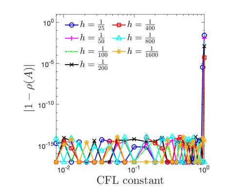
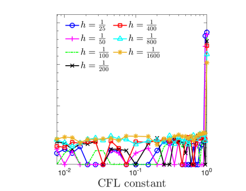
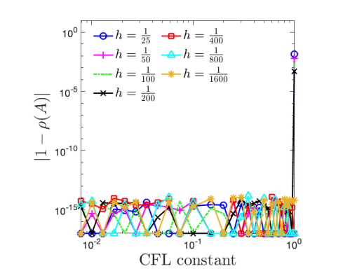
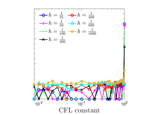
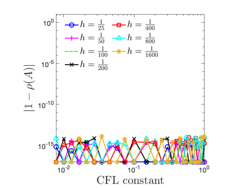
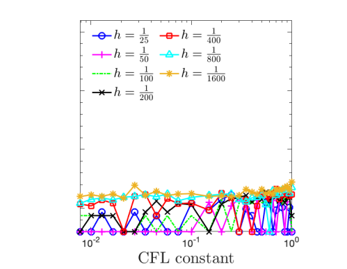
Figure 11: Absolute difference between one and the spectral radius $\rho(A)$ of the matrix $A$ as a function of the CFL constant for different mesh sizes. We use $m=1$ and $m=2$ for respectively the left and right plots. The top, middle and bottom rows are respectively for $c_{H}=\frac{1}{2}$, $c_{H}=\frac{1}{10}$ and $c_{H}=\frac{1}{50}$.

Note that the CFL constant under which the method is stable increases as the mesh size diminishes. Hence, the parameter $c_{H}$ can be chosen using a coarser mesh and should remain appropriate for finer meshes.

As $c_{H}$ decreases, the stability condition of the Hermite-Taylor correction method tends to be $\Delta t\leq h$, corresponding to the stability condition of the Hermite-Taylor method, as better illustrated in Fig. 12.

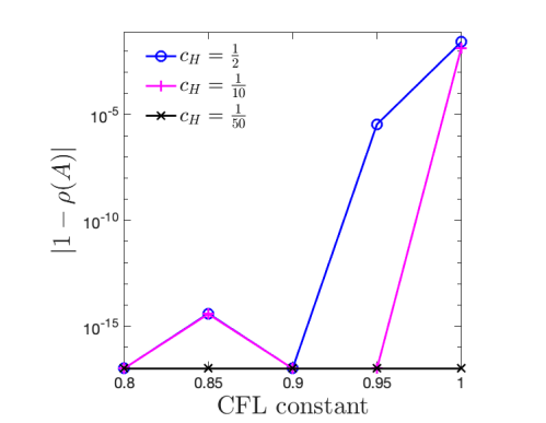
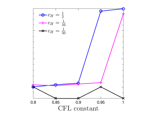
Figure 12: Absolute difference between one and the spectral radius $\rho(A)$ of the matrix $A$ as a function of the CFL constant for $h=\frac{1}{25}$ and using different penalization coefficients $c_{H}$. We use $m=1$ and $m=2$ for respectively the left and right plots.

For $m\geq 3$, it was observed that there is a lower bound on the CFL constant under which the method becomes unstable similar to what was reported in LawAppelo2022 . We therefore focus on $m\in\{1,2\}$.

Let us consider a domain where there are primal and dual CF nodes. The physical domain $\Omega=[\frac{\pi}{50},1-\frac{\pi}{100}]$ while the computational domain is $\Omega_{c}=[0,1]$. In this situation, the method cannot be written as (16) because the evolution of the data from $t_{n}$ to $t_{n+1}$ requires the numerical solutions at times $t_{n-1/2}$ and $t_{n}$ for the dual CF nodes, and times $t_{n}$ and $t_{n+1/2}$ for the primal CF nodes. We therefore investigate the stability using long time simulations. We consider the trivial solution for all electromagnetic fields but with initial data, namely the electromagnetic fields and their first $m$ derivatives, to be random numbers in $]-10\,\epsilon_{m},10\,\epsilon_{m}[$. Here $\epsilon_{m}$ is the machine precision.

Fig. 13 illustrates the maximum norm of the numerical solution over 5,000 time steps for different mesh sizes, $m\in\{1,2\}$ and $c_{H}\in\{\frac{1}{2},\frac{1}{10},\frac{1}{50}\}$.

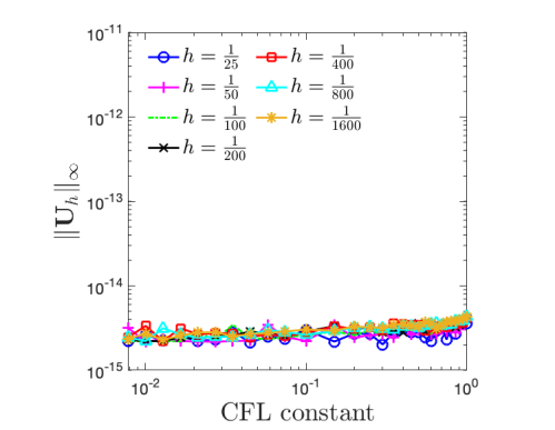
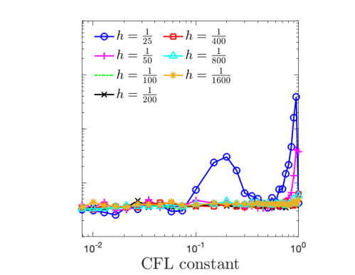
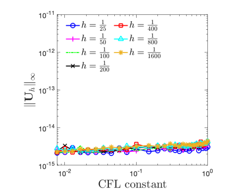
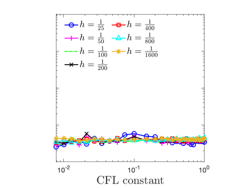
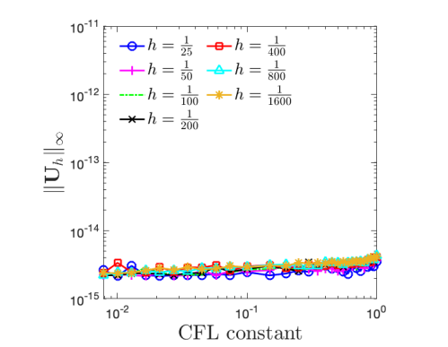
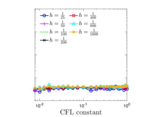
Figure 13: Maximum value of the maximum norm of the numerical solution over 5,000 time steps as a function of the CFL constant for different mesh sizes. We use $m=1$ and $m=2$ for the left and right plots respectively. The top, middle and bottom rows are respectively for $c_{H}=\frac{1}{2}$, $c_{H}=\frac{1}{10}$ and $c_{H}=\frac{1}{50}$. Here $\mathbold{U}=[H,E]^{T}$.

Here again the stability condition of the Hermite-Taylor correction function methods tends to $\Delta t\leq h$ as $c_{H}$ and the mesh size decrease.

5.1.2 Condition Number of CFM Matrices

Let us now investigate the impact of $c_{H}$, the CFL constant and the mesh size on the condition number of the correction function matrices. We consider the physical domain $\Omega=[h_{\max}-\frac{h_{\min}}{3},1-h_{\max}+\frac{5\,h_{\min}}{12}]$ and the computational domain $\Omega_{c}=[0,1]$. Here $h\in\{\frac{1}{25},\frac{1}{50},\frac{1}{100},\frac{1}{200},\frac{1}{400},\frac{1}{800},\frac{1}{1600}\}$. Note that all the CF nodes belong to the primal mesh.

Fig. 14 illustrates the maximum condition number as a function of the CFL constant for different mesh sizes, $c_{H}\in\{\frac{1}{2},\frac{1}{10},\frac{1}{50}\}$ and $m\in\{1,2\}$.

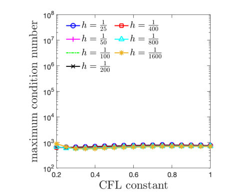
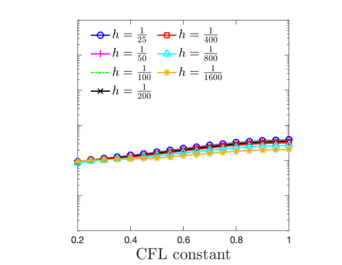
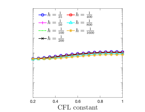
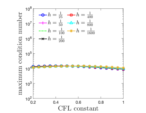
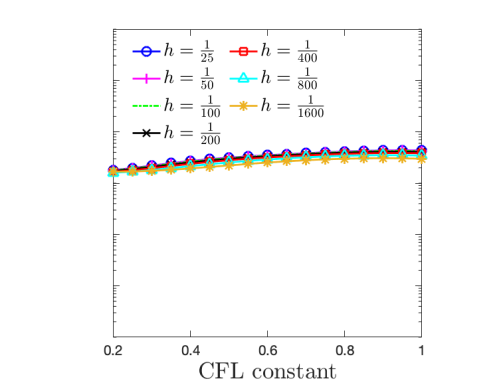
Figure 14: Maximum condition number of CF matrices as a function of the CFL constant for different mesh sizes. We use $m=1$ and $m=2$ for respectively the left and right plots. The top, middle and bottom rows are respectively for $c_{H}=\frac{1}{2}$, $c_{H}=\frac{1}{10}$ and $c_{H}=\frac{1}{50}$.

The maximum condition number remains roughly the same as the mesh size and the CFL constant decrease. This is an improvement over the Hermite-Taylor correction function method developed in LawAppelo2022 to handle boundary conditions, where the condition number increases as the mesh size and the CFL constant diminish.

As $c_{H}$ decreases, the condition number increases as $\mathcal{O}(\frac{1}{c_{H}})$ as illustrated in the left plot of Fig. 15.

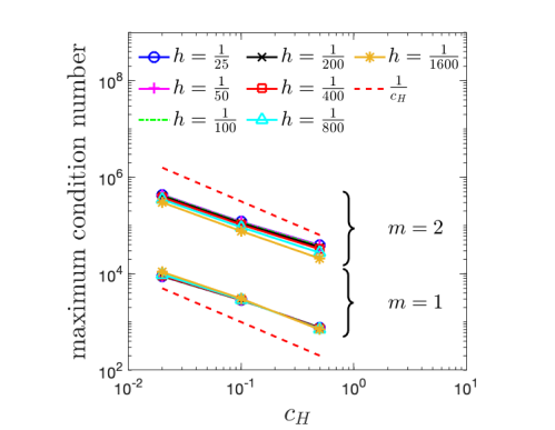
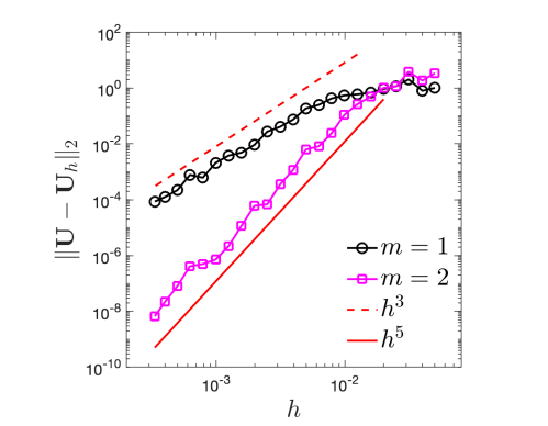
Figure 15: The left plot shows the maximum condition number of the CF matrices as a function of $c_{H}$ for different mesh sizes. Here the CFL constant is 1. The right plot shows the convergence plots for embedded boundary problems using the third and fifth order Hermite-Taylor correction function methods. Here $\mathbf{U}=[H,E]^{T}$.

As mentioned in Remark 3, the value of $c_{H}$ cannot be taken arbitrary small to avoid a large condition number of the correction function matrices.

5.1.3 Accuracy

Let us now investigate the accuracy of the Hermite-Taylor correction function method with $m\in\{1,2\}$. The physical parameters are $\mu=1$ and $\epsilon=1$. We set $c_{H}=\tfrac{1}{10}$ and $\Delta t=0.9\,h$.

The physical domain is $\Omega=[\frac{\pi}{50},1-\frac{\pi}{100}]$ while the computational domain is $\Omega_{c}=[0,1]$. The time interval is $I=[0,20]$. The initial and boundary conditions are chosen so that the solution to Maxwell’s equations is

$$H(x,t)= \,\,\sin(250\,x)\,\sin(250\,t),$$

$$E(x,t)= \,\,\cos(250\,x)\,\cos(250\,t).$$

The error in the $L^{2}$-norm is computed at the final time. The right plot of Fig. 15 illustrates the convergence plots for $m\in\{1,2\}$. As expected, we observe a third-order convergence for $m=1$ and a fifth-order convergence for $m=2$.

5.2 Hermite-Taylor Correction Function Methods in Two Dimensions

We consider the two-dimensional simplification of Maxwell’s equations (5). The correction function polynomials are chosen to be elements of $\mathbb{Q}^{2\,m}$ to preserve the accuracy of the Hermite-Taylor method. We choose $\beta=5$ for the dimension of the square spatial domain of the local patches.

5.3 Stability

In this subsection, we investigate the stability of the Hermite-Taylor correction function method for embedded boundary and interface problems. To do so, we use long time simulations.

5.3.1 Embedded Boundary Problems

We consider the computational domain $\Omega_{c}=[0,1]\times[0,1]$, illustrated in Fig. 16.

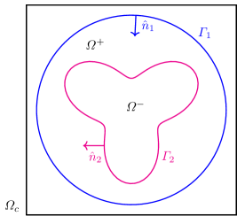
Figure 16: Geometry of the computational domain $\Omega_{c}$.

Here $\Gamma_{1}$ and $\Gamma_{2}$ are boundaries of the domain $\Omega^{+}$ where we seek a numerical solution.

As in the one-dimensional experiments described above, we consider the trivial solution for all electromagnetic fields but with initial data, namely the electromagnetic fields and the necessary derivatives, to be random numbers in $]-10\,\epsilon_{m},10\,\epsilon_{m}[$. The physical parameters are set to $\mu=1$ and $\epsilon=1$.

Fig. 17 illustrates the evolution of the maximum norm of the numerical solution over 10,000 time steps for $m\in\{1,2\}$, different mesh sizes and $c_{H}\in\{\frac{1}{2},\frac{1}{10},\frac{1}{50}\}$. We use a CFL constant of 0.9 and 0.5 for respectively $m=1$ and $m=2$.

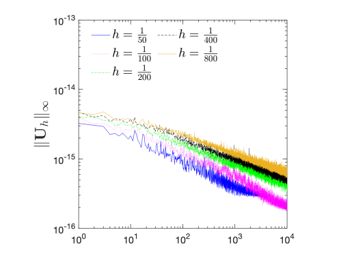
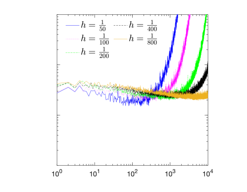
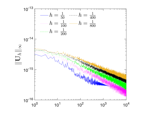
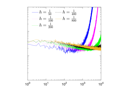
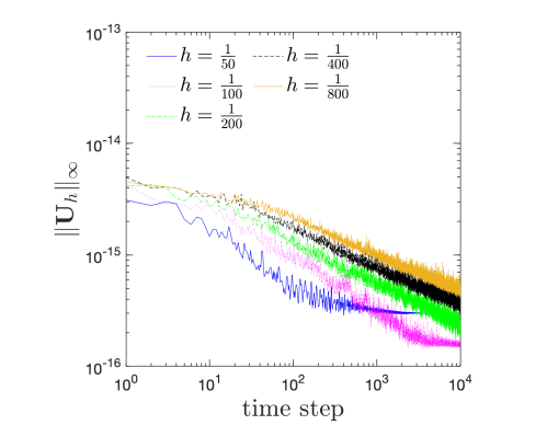
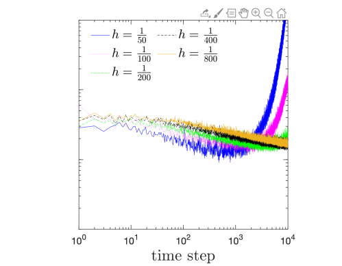
Figure 17: Evolution of the maximum norm of the numerical solution as a function of the time steps for different mesh sizes and penalization coefficients $c_{H}$. We use $m=1$ and $m=2$ for the left and right plots respectively. The top, middle and bottom rows are respectively for $c_{H}=\frac{1}{2}$, $c_{H}=\frac{1}{10}$ and $c_{H}=\frac{1}{50}$. Here $\mathbold{U}=[H_{x},H_{y},E_{z}]^{T}$.

For $m=1$, the Hermite-Taylor correction function method is stable for all considered penalization coefficients and all mesh sizes. As for $m=2$, the stability of the Hermite-Taylor correction function method is more sensitive to the penalization coefficients. The stability improves as the mesh size and the parameter $c_{H}$ decrease.

According to the numerical results, the parameter $c_{H}$ can be chosen using a coarser mesh and should remain appropriate for finer meshes.

5.3.2 Interface Problems

Let us now consider interface problems. We investigate the stability using the same setup as for the embedded boundary problems. In this situation, $\Gamma_{2}$ is an interface while $\Gamma_{1}$ is still an embedded boundary for $\Omega^{+}$. We are seeking a numerical solution in $\Omega^{+}$ and $\Omega^{-}$. We consider $\mu^{+}=1$, $\epsilon^{+}=1$, $\mu^{-}=2$ and $\epsilon^{-}=2.25$ .

Fig. 18 illustrates the evolution of the maximum norm of the numerical solution over 10,000 time steps for $m\in\{1,2\}$, different mesh sizes and $c_{H}\in\{\frac{1}{2},\frac{1}{10},\frac{1}{50}\}$.

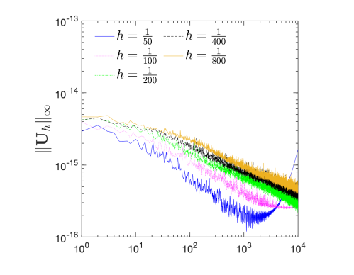
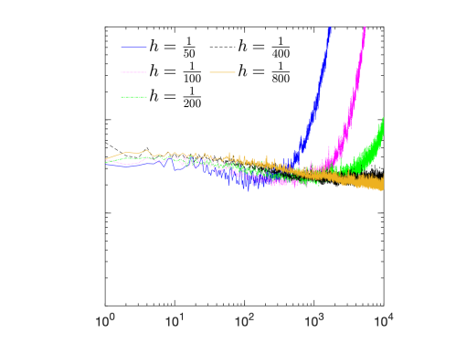
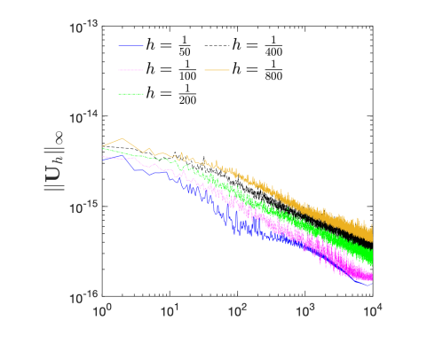
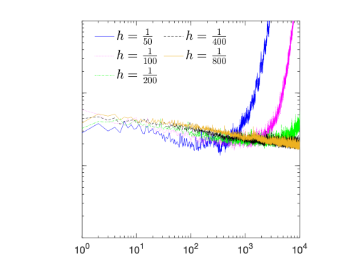
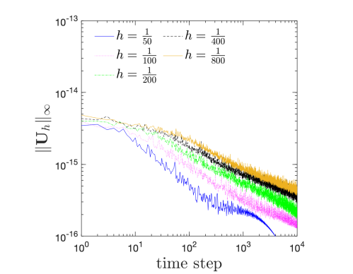
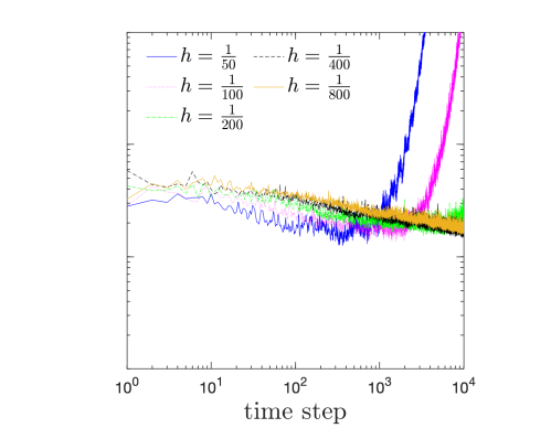
Figure 18: Evolution of the maximum norm of the numerical solution as a function of the time steps for different mesh sizes and value of $c_{H}$. We use $m=1$ and $m=2$ for the left and right plots respectively. The top, middle and bottom rows are respectively for $c_{H}=\frac{1}{2}$, $c_{H}=\frac{1}{10}$ and $c_{H}=\frac{1}{50}$. Here $\mathbold{U}=[H_{x},H_{y},E_{z}]^{T}$.

Here also the stability of the Hermite-Taylor correction function method improves as the mesh size and the parameter $c_{H}$ decrease.

5.4 Condition Number of the CFM matrices

Let us now investigate the condition number of the correction function matrices for embedded boundaries and interfaces. Fig. 19 shows the maximum condition number of CF matrices as a function of the mesh size using $c_{H}\in\{\frac{1}{2},\frac{1}{10},\frac{1}{50}\}$.

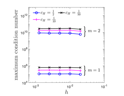
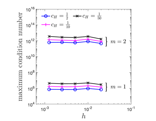
Figure 19: Maximum condition number of CF matrices as a function of the mesh size using different penalization coefficients $c_{H}$. The left and right plots are respectively for the embedded boundary problem and the interface problems. Note that the dual CF matrices of the first time step are not considered here.

The maximum condition number remains roughly the same for all mesh sizes for the embedded boundary and interface problems. However, the condition number increases when an interface is considered. This is expected since the dimension of the CF matrices to treat interfaces is twice larger than the CF matrices for embedded boundaries.

Fig. 20 shows the maximum condition number as a function of the parameter $c_{H}$.

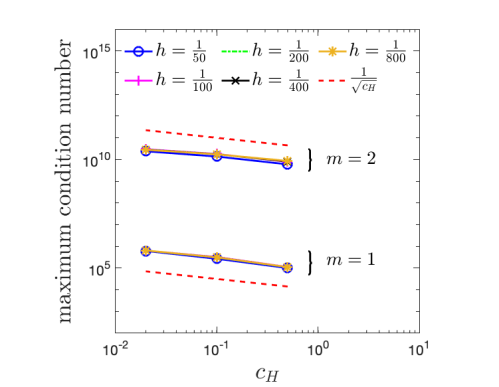
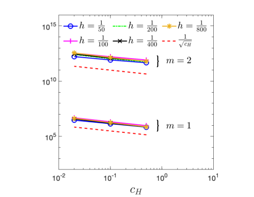
Figure 20: Maximum condition number of CF matrices as a function of the parameter $c_{H}$ using different mesh sizes. The left and right plots are respectively for the embedded boundary problem and the interface problems. Note that the dual CF matrices of the first time step are not considered here.

As the parameter $c_{H}$ decreases, the condition number increases as $\mathcal{O}(\frac{1}{\sqrt{c_{H}}})$ for embedded boundaries as well as interfaces. Again the value of $c_{H}$ cannot be taken arbitrary small because of its impact on the condition number of the CF matrices. That being said, the parameter $c_{H}$ can be chosen using a coarser mesh and should remain appropriate for finer meshes.

5.5 Accuracy

Let us now investigate the accuracy of the Hermite-Taylor correction function method. We set the parameter $c_{H}=\frac{1}{50}$. Since the degree of the correction function polynomials is $2\,m$, we should expect third and fifth order convergence, respectively, for Hermite-Taylor correction function methods with $m=1$ and $m=2$. We use a CFL constant of 0.9 and 0.5 for the third and fifth order Hermite-Taylor correction function methods.

5.5.1 Embedded Boundary Problems

The first example consists of a circular cavity problem. The computational domain is $\Omega_{c}=[-1.1,1.1]\times[-1.1,1.1]$ and the embedded boundary $\Gamma$ is a circle of unit radius and centered at $(0,0)$ that encloses the physical domain $\Omega$. The time interval is $I=[0,1]$ and we enforce PEC boundary conditions on $\Gamma$. The physical parameters are $\epsilon=1$ and $\mu=1$, and the solution in cylindrical coordinates in $\Omega$ is given by

$$H_{\rho}(\rho,\phi,t)= \,\,\frac{i}{\alpha_{i,j}\,\rho}\,J_{i}(\alpha_{i,j}\,\rho)\,\sin(i\,\phi)\,\sin(\alpha_{i,j}\,t),$$

$$H_{\phi}(\rho,\phi,t)= \,\,\frac{1}{2}\,\big{(}J_{i-1}(\alpha_{i,j}\,\rho)-J_{i+1}(\alpha_{i,j}\,\rho)\big{)}\,\cos(i\,\phi)\,\sin(\alpha_{i,j}\,t),$$

$$E_{z}(\rho,\phi,t)= \,\,J_{i}(\alpha_{i,j}\,\rho)\,\cos(i\,\phi)\,\cos(\alpha_{i,j}\,t),$$

where $\alpha_{i,j}$ is the $j$-th positive real root of the $i$-order Bessel function of first kind $J_{i}$, $i=2$ and $j=11$. The left plot of Fig. 22 shows that we obtain the expected $2\,m+1$ rates of convergence in the $L^{2}$-norm. Fig. 21 illustrates the approximations of electromagnetic fields at the final time.

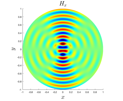
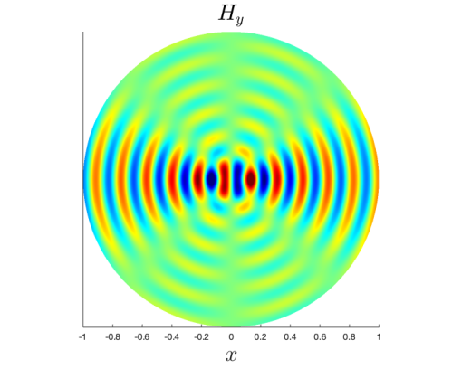
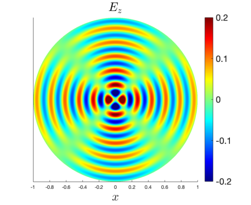
Figure 21: The components $H_{x}$, $H_{y}$ and $E_{z}$ at the final time $t_{f}=1$ for a circular cavity problem using the fifth-order Hermite-Taylor correction function method and $h=\frac{1}{460}$.

We now consider the computational domain $\Omega_{c}=[0,1]\times[0,1]$, illustrated in Fig. 16, and the time interval is $I=[0,1]$. In this situation, we are seeking a numerical solution in $\Omega^{+}$. The physical parameters are $\mu=1$ and $\epsilon=1$. The initial data, and boundary conditions on $\Gamma_{1}$ and $\Gamma_{2}$ are chosen so that the solution in $\Omega^{+}$ is given by

$$H_{x}= \,\,-\frac{1}{\sqrt{2}}\sin(\omega\,\pi\,x)\,\cos(\omega\,\pi\,y)\,\sin(\sqrt{2}\,\omega\,\pi\,t),$$

$$H_{y}= \,\,\frac{1}{\sqrt{2}}\cos(\omega\,\pi\,x)\,\sin(\omega\,\pi\,y)\,\sin(\sqrt{2}\,\omega\,\pi\,t),$$

$$E_{z}= \,\,\sin(\omega\,\pi\,x)\,\sin(\omega\,\pi\,y)\,\cos(\sqrt{2}\,\omega\,\pi\,t),$$

where $\omega=20$. The right plot of Fig. 22 shows the convergence plots in the $L^{2}$-norm for $m=1$ and $m=2$.

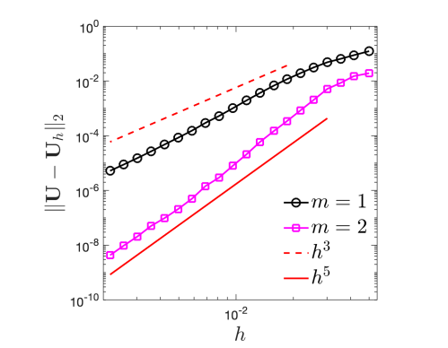
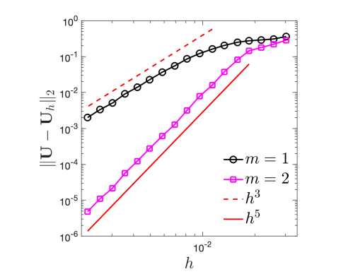
Figure 22: Convergence plots for embedded boundary problems using the third and fifth order Hermite-Taylor correction function methods. For the left plot, we consider a circular cavity problem. For the right plot, we consider an embedded boundaries problem with the geometry illustrated in Fig. 16. Here $\mathbf{U}=[H_{x},H_{y},E_{z}]^{T}$.

In both cases, we observe the expected $2\,m+1$ convergence rates. The approximations of electromagnetic fields at the final time are illustrated in Fig. 23.

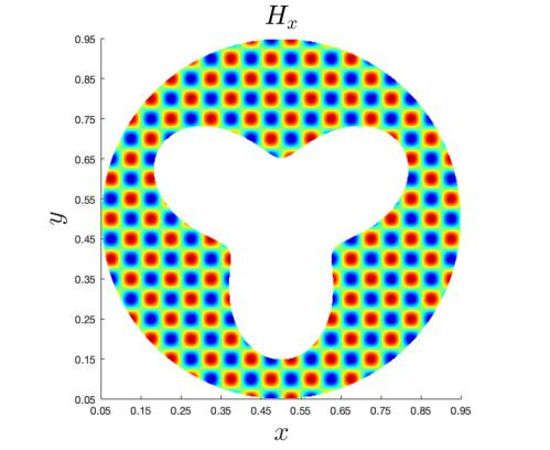
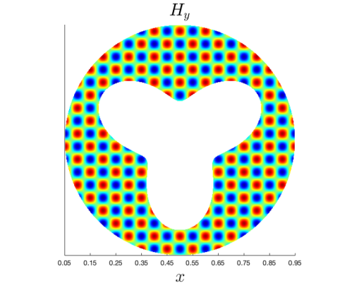
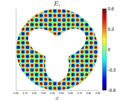
Figure 23: The components $H_{x}$, $H_{y}$ and $E_{z}$ at the final time $t_{f}=1$ for an embedded boundary problem with the geometry illustrated in Fig. 16 using the fifth-order Hermite-Taylor correction function method and $h=\frac{1}{460}$.

5.5.2 Interface Problems with Analytic Solutions

Let us now consider Maxwell’s interface problems. First, we consider a dielectric cylinder in free-space exposed to an excitation wave. The geometry of the computational domain consists of two concentric circles enclosed in $\Omega_{c}=[-1,1]\times[-1,1]$. The first circle centered at $(0,0)$ has a radius of 0.8 and is an embedded boundary $\Gamma_{1}$ of $\Omega^{+}$. The second circle also centered at $(0,0)$, but with a radius $r_{0}=0.6$, which represents the interface $\Gamma_{2}$ between the subdomains and enclosed the subdomain $\Omega^{-}$. The time interval is set to $I=[0,1]$.

The initial and boundary conditions are chosen such that the solution in cylindrical coordinates is given by the real part of

$$H_{\theta}(r,\theta,t)= \,\,\left\{\begin{array}[]{l l}-\frac{\mathfrak{i}\,k^{-}}{\omega\,\mu^{-}}\displaystyle\sum_{n=-\infty}^{\infty}C_{n}^{\text{tot}}\,J_{n}^{\prime}(k^{-}\,r)\,e^{\mathfrak{i}\,(n\,\theta+\omega\,t)},&\text{if}\quad r\leq r_{0},\\ -\frac{\mathfrak{i}\,k^{+}}{\omega\,\mu^{+}}\displaystyle\sum_{n=-\infty}^{\infty}(\mathfrak{i}^{-n}\,J_{n}^{\prime}(k^{+}\,r)+C_{n}^{\text{scat}}\,H_{n}^{{(2)}^{\prime}}(k^{+}\,r))\,e^{\mathfrak{i}\,(n\,\theta+\omega\,t)},&\text{if}\quad r>r_{0},\end{array}\right.$$

$$H_{r}(r,\theta,t)= \,\,\left\{\begin{array}[]{l l}-\frac{1}{\omega\,\mu^{-}\,r}\displaystyle\sum_{n=-\infty}^{\infty}n\,C_{n}^{\text{tot}}\,J_{n}(k^{-}\,r)\,e^{\mathfrak{i}\,(n\,\theta+\omega\,t)},&\text{if}\quad r\leq r_{0},\\ -\frac{1}{\omega\,\mu^{+}\,r}\displaystyle\sum_{n=-\infty}^{\infty}n\,(\mathfrak{i}^{-n}\,J_{n}(k^{+}\,r)+C_{n}^{\text{scat}}\,H_{n}^{(2)}(k^{+}\,r))\,e^{\mathfrak{i}\,(n\,\theta+\omega\,t)},&\text{if}\quad r>r_{0},\end{array}\right.$$

$$E_{z}(r,\theta,t)= \,\,\left\{\begin{array}[]{l l}\displaystyle\sum_{n=-\infty}^{\infty}C_{n}^{\text{tot}}\,J_{n}(k^{-}\,r)\,e^{\mathfrak{i}\,(n\,\theta+\omega\,t)},&\text{if}\quad r\leq r_{0},\\ \displaystyle\sum_{n=-\infty}^{\infty}(\mathfrak{i}^{-n}\,J_{n}(k^{+}\,r)+C_{n}^{\text{scat}}\,H_{n}^{(2)}(k^{+}\,r))\,e^{\mathfrak{i}\,(n\,\theta+\omega\,t)},&\text{if}\quad r>r_{0},\end{array}\right.$$

with

$$C_{n}^{\text{tot}}= \,\,\mathfrak{i}^{-n}\,\frac{\tfrac{k^{+}}{\mu^{+}}\,(J_{n}^{\prime}(k^{+}\,r_{0})\,H_{n}^{(2)}(k^{+}\,r_{0})-H_{n}^{{(2)}^{\prime}}(k^{+}\,r_{0})\,J_{n}(k^{+}\,r_{0}))}{\frac{k^{-}}{\mu^{-}}\,J_{n}^{\prime}(k^{-}\,r_{0})\,H_{n}^{(2)}(k^{+}\,r_{0})-\tfrac{k^{+}}{\mu^{+}}\,H_{n}^{{(2)}^{\prime}}(k^{+}\,r_{0})\,J_{n}(k^{-}\,r_{0})},$$

$$C_{n}^{\text{scat}}= \,\,\mathfrak{i}^{-n}\,\frac{\tfrac{k^{+}}{\mu^{+}}\,J_{n}^{\prime}(k^{+}\,r_{0})\,J_{n}(k^{-}\,r_{0})-\tfrac{k^{-}}{\mu^{-}}\,J_{n}^{\prime}(k^{-}\,r_{0})\,J_{n}(k^{+}\,r_{0})}{\frac{k^{-}}{\mu^{-}}\,J_{n}^{\prime}(k^{-}\,r_{0})\,H_{n}^{(2)}(k^{+}\,r_{0})-\tfrac{k^{+}}{\mu^{+}}\,H_{n}^{{(2)}^{\prime}}(k^{+}\,r_{0})\,J_{n}(k^{-}\,r_{0})}.$$

Here $\omega=2\,\pi$, $k^{\circ}=\omega\,\sqrt{\mu^{\circ}\,\epsilon^{\circ}}$, $J_{n}$ is the $n$-order Bessel function of first kind and $H_{n}^{(2)}$ is the $n$-order Hankel function of second kind and the imaginary number is $\mathfrak{i}$ Taflove1993 ; Cai2003 .

We set $\mu^{+}=1$, $\epsilon^{+}=1$, $\mu^{-}=2$ and $\epsilon^{-}=2.25$. Hence, $\Omega^{-}$ is a magnetic dielectric material. In this situation, $H_{x}$ and $H_{y}$ are discontinuous at the interface and $E_{z}$ is continuous.

As shown in Fig. 24, we observe the expected $2\,m+1$ rates of convergence, even in the presence of discontinuities.

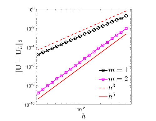
Figure 24: Convergence plots for the scattering of a magnetic dielectric cylinder problem using the third and fifth order Hermite-Taylor correction function methods. Here $\mathbf{U}=[H_{x},H_{y},E_{z}]^{T}$.

The approximations of electromagnetic fields at the final time are illustrated in Fig. 25.

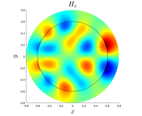
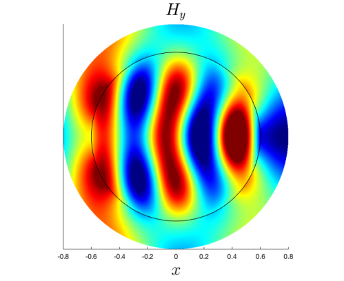
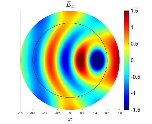
Figure 25: The components $H_{x}$, $H_{y}$ and $E_{z}$ at the final time $t_{f}=1$ for the scattering of a magnetic dielectric problem using the fifth-order Hermite-Taylor correction function method and $h=\frac{1}{460}$. The interface is represented by the black line.

Fig. 26 illustrates the magnetic field components at $y=0.2$ along $x$.

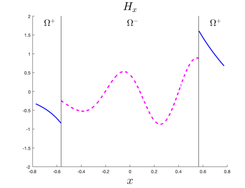
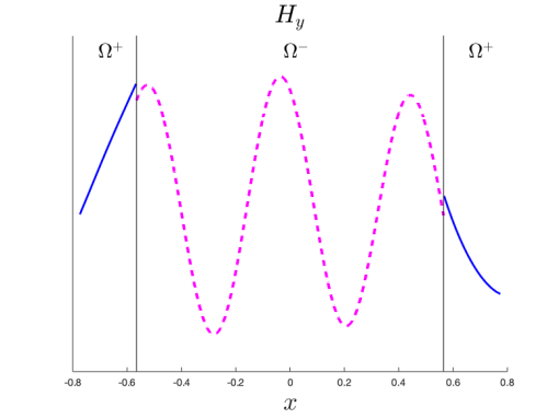
Figure 26: The components $H_{x}$ and $H_{y}$ at $y=0.2$ and the final time $t_{f}=1$ for the scattering of a magnetic dielectric problem using the fifth-order Hermite-Taylor correction function method and $h=\frac{1}{460}$. The interface is represented by the vertical black line. The numerical solution in $\Omega^{+}$ and $\Omega^{-}$ are respectively represented by the blue line and the dashed magenta line.

The discontinuities at the interface are well captured by the Hermite-Taylor correction function method.

5.6 Interface Problems with Reference Solutions

We now consider the computational domain illustrated in Fig. 16 with $\Omega_{c}=[0,1]\times[0,1]$ and a time interval $I=[0,1]$. We set $\mu^{+}=1$, $\epsilon^{+}=1$, $\mu^{-}=2$ and $\epsilon^{-}=2.25$ so $H_{x}$ and $H_{y}$ could be discontinuous at the interface. The boundary condition on $\Gamma_{1}$ is given by

$$E_{z}(t)=e^{-\frac{(t-0.3)^{2}}{2\,\sigma^{2}}},$$

while interface conditions (4) are enforced on $\Gamma_{2}$. Here $\sigma=0.02$. The initial conditions are given by trivial electromagnetic fields.

To our knowledge, there is no analytical solution to this problem. Hence, we compute a reference solution $\mathbold{U}^{*}$ with a very refined mesh, that is $h=\tfrac{1}{1600}$, and the fifth-order Hermite-Taylor correction function method. The reference solution is illustrated in Fig. 27.

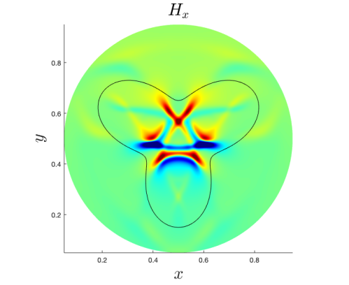
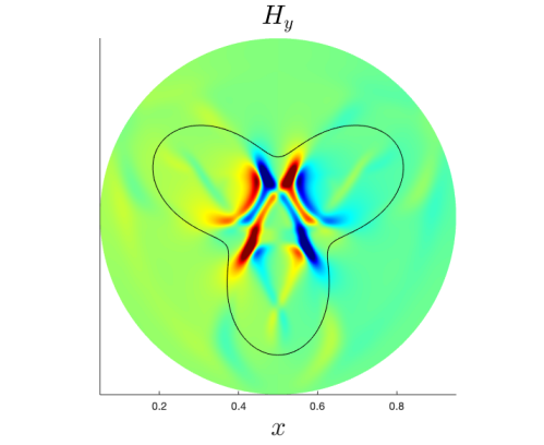
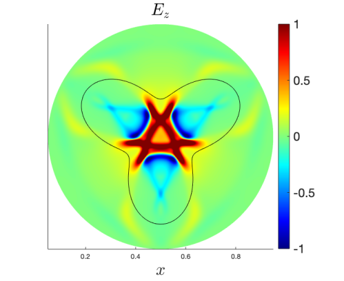
Figure 27: The components $H_{x}$, $H_{y}$ and $E_{z}$ at the final time $t_{f}=1$ for an interface problem with the geometry illustrated in Fig. 16 using the fifth-order Hermite-Taylor correction function method and $h=\frac{1}{1600}$. We consider a Gaussian pulse in time as the boundary condition for $E_{z}$. The interface is represented by the black line.

Afterward, we estimate the errors by comparing the reference solution to approximations coming from meshes with $h\in\{\tfrac{1}{25},\tfrac{1}{50},\tfrac{1}{100},\tfrac{1}{200},\tfrac{1}{400},\tfrac{1}{800}\}$. Note that all primal nodes for these meshes are also part of the reference solution mesh.

The error in the $L^{2}$-norm is computed at the final time. The left plot of Fig. 28 illustrates that we obtain the expected $2\,m+1$ rates of convergence.

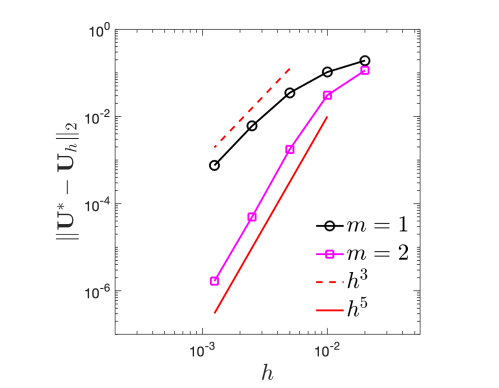
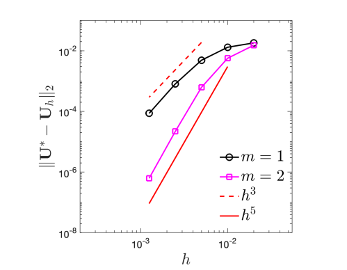
Figure 28: Self convergence plots for interface problems with the geometry illustrated in Fig. 16 using the third and fifth order Hermite-Taylor correction function methods. For the left plot, we consider a Gaussian pulse in time as the boundary condition for $E_{z}$. For the right plot, we consider a Gaussian pulse as an initial condition for $E_{z}$. Here $\mathbf{U}=[H_{x},H_{y},E_{z}]^{T}$.

As a final example, we consider the same geometry where we enforce PEC boundary conditions on $\Gamma_{1}$. The initial conditions are $H_{x}=H_{y}=0$ and

$$E_{z}(x,y)=e^{\frac{-(x-0.5)^{2}-(y-0.5)^{2}}{2\,\sigma^{2}}}.$$

Here $\sigma=0.01$. In this situation, we are not aware of an analytical solution. We then perform self convergence studies using the reference solution, illustrated in Fig. 29, that has been computed with $h=\frac{1}{1600}$ using the fifth-order Hermite-Taylor correction function method.

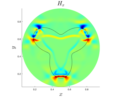
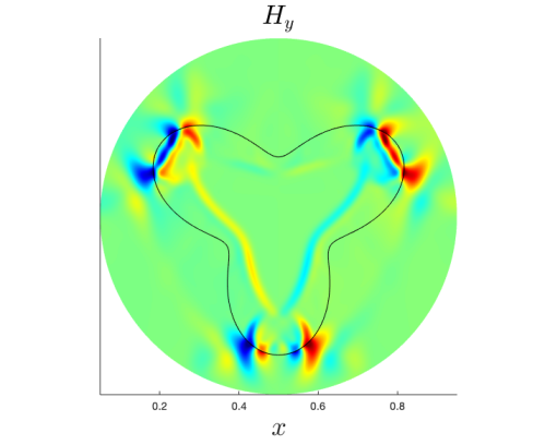
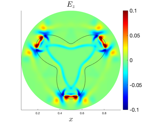
Figure 29: The components $H_{x}$, $H_{y}$ and $E_{z}$ at the final time $t_{f}=1$ for an interface problem with the geometry illustrated in Fig. 16 using the fifth-order Hermite-Taylor correction function method and $h=\frac{1}{1600}$. We consider a Gaussian pulse as an initial condition for $E_{z}$. The interface is represented by the black line.

The right plot of Fig. 28 illustrates the self convergence plots in the $L^{2}$-norm. We obtain the expected $2\,m+1$ rates of convergence.

6 Conclusion

In this work, we have proposed a novel Hermite-Taylor correction function method to handle embedded boundary and interface conditions for Maxwell’s equations. We take advantage of the correction function method to update the numerical solution at the nodes where the Hermite-Taylor method cannot be applied. To do so, we minimize a functional that is a square measure of the residual of Maxwell’s equations, the boundary or interface conditions, and the polynomials approximating the electromagnetic fields coming from the Hermite-Taylor method. The approximations of the electromagnetic fields and their required derivatives are then updated using the correction functions resulting from the minimization procedure. Numerical examples suggest that the third and fifth order Hermite-Taylor correction function methods are stable under a reasonable CFL constraint and value of the penalization coefficient. The accuracy of the Hermite-Taylor correction function method was verified. The proposed method achieves high order accuracy even with interface problems with discontinuous solutions. Finally, this method can be easily adapted to other first order hyperbolic problems.

Declarations

Funding

This work was supported in part by NSF Grants DMS-2208164, DMS-2210286 and DMS-2012296. Any opinions, findings, and conclusions or recommendations expressed in this material are those of the authors and do not necessarily reflect the views of the NSF.

Conflicts of interest/Competing interests

On behalf of all authors, the corresponding author states that there is no conflict of interest.

References

- (1) Abraham, D.S., Marques, A.N., Nave, J.C.: A correction function method for the wave equation with interface jump conditions. J. Comput. Phys. 353, 281–299 (2018)
- (2) Banks, J.W., Buckner, B.B., Henshaw, W.D., Jenkinson, M.J., Kildishev, A.V., Kovačič, G., Prokopeva, L.J., Schwendeman, D.W.: A high-order accurate scheme for Maxwell’s equations with a Generalized Dispersive Material (GDM) model and material interfaces. J. Comput. Phys. 412, 109424 (2020)
- (3) Beznosov, O., Appelö, D.: Hermite - discontinuous Galerkin overset grid methods for the scalar wave equation. Communications on Applied Mathematics and Computation (2020)
- (4) Cai, W., Deng, S.: An upwinding embedded boundary method for Maxwell’s equations in media with material interfaces: 2D case. J. Comput. Phys. 190, 159–183 (2003)
- (5) Chen, W., Li, X., Liang, D.: Energy-conserved splitting finite-difference time-domain methods for Maxwell’s equations in three dimensions. SIAM J. Numer. Anal. 48, 1530–1554 (2010)
- (6) Cockburn, B., Shu, C.W.: Runge–kutta discontinuous Galerkin methods for convection-dominated problems. Journal of Scientific Computing 16(3), 173–261 (2001)
- (7) Ditkowski, A., Dridi, K., Hesthaven, J.S.: Convergent Cartesian grid methods for Maxwell equations in complex geometries. J. Comput. Phys. 170, 39–80 (2001)
- (8) Driscoll, T.A., Fornberg, B.: Block pseudospectral methods for Maxwell’s equations II: two-dimensional, discontinuous-coefficient case. SIAM J. Sci. Comput. 21, 1146–1167 (1999)
- (9) Fan, G.X., Liu, Q.H., Hesthaven, J.S.: Multidomain pseudospectral time-domain simulations of scattering by objects buried in lossy media. IEEE Trans. Geosci. Remote Sens. 40, 1366–1373 (2002)
- (10) Galagusz, R., Shirokoff, D., Nave, J.C.: A Fourier penalty method for solving the time-dependent Maxwell’s equations in domains with curved boundaries. J. Comput. Phys. 306, 167–198 (2016)
- (11) Goodrich, J., Hagstrom, T., Lorenz, J.: Hermite methods for hyperbolic initial-boundary value problems. Math. Comp. 75, 595–630 (2005)
- (12) Hesthaven, J.S.: High-order accurate methods in time-domain computational electromagnetics: a review. Adv. Imag. Electron Phys. 127, 59–123 (2003)
- (13) Hesthaven, J.S., Warburton, T.: Nodal high-order methods on unstructured grids: I. time-domain solution of Maxwell’s equations. J. Comput. Phys. 181, 186–221 (2002)
- (14) Law, Y.M., Appelö, D.: The Hermite-Taylor correction function method for Maxwell’s equations. arXiv preprint arXiv:2210.07134 (2022)
- (15) Law, Y.M., Marques, A.N., Nave, J.C.: Treatment of complex interfaces for Maxwell’s equations with continuous coefficients using the correction function method. J. Sci. Comput. 82(3), 56 (2020)
- (16) Law, Y.M., Nave, J.C.: FDTD schemes for Maxwell’s equations with embedded perfect electric conductors based on the correction function method. J. Sci. Comput. 88(3), 72 (2021)
- (17) Law, Y.M., Nave, J.C.: High-order FDTD schemes for Maxwell’s interface problems with discontinuous coefficients and complex interfaces based on the correction function method. J. Sci. Comput. 91(1), 26 (2022)
- (18) Loya, A.A., Appelö, D., Henshaw, W.D.: Hermite methods for the wave equation: Compatibility and interface conditions. in preparation (2022)
- (19) Marques, A.N., Nave, J.C., Rosales, R.R.: A correction function method for Poisson problems with interface jump conditions. J. Comput. Phys. 230, 7567–7597 (2011)
- (20) Marques, A.N., Nave, J.C., Rosales, R.R.: High order solution of Poisson problems with piecewise constant coefficients and interface jumps. J. Comput. Phys. 335, 497–515 (2017)
- (21) Taflove, A.: Computational electrodynamics : the finite difference time-domain method. Artech House (1995)
- (22) Yang, B., Gottlieb, D., Hesthaven, J.S.: Spectral simulations of electromagnetic wave scattering. J. Comput. Phys. 134, 216–230 (1997)
- (23) Zhang, Y., Nguyen, D.D., Du, K., Xu, J., Zhao, S.: Time-domain numerical solutions of Maxwell interface problems with discontinuous electromagnetic waves. Adv. Appl. Math. Mech. 8, 353–385 (2016)
- (24) Zhao, S., Wei, G.W.: High-order FDTD methods via derivative matching for Maxwell’s equations with material interfaces. J. Comput. Phys. 200, 60–103 (2004)