An efficient and quantitative phase-field model for elastically heterogeneous two-phase solids based on a partial rank-one homogenization scheme
bDepartment of Materials Science and Engineering, University of Florida, Gainesville, 32611, FL, USA
cComputational Mechanics and Materials Department, Idaho National Laboratory, Idaho Falls, ID 83415, United States
∗Corresponding author. E-mail addresses:
soran.chatterjee@gmail.com (S. Chatterjee), daniel.schwen@inl.gov (D. Schwen), nele.moelans@kuleuven.be (N. Moelans) )
Abstract
This paper presents an efficient and quantitative phase-field model for elastically heterogeneous alloys that ensures the two mechanical compatibilities—static and kinematic, in conjunction with chemical equilibrium within the interfacial region. Our model contrasts with existing phase-field models that either violate static compatibility or interfacial chemical equilibrium or are computationally costly. For computational efficiency, the partial rank-one homogenization (PRH) scheme is employed to enforce both static and kinematic compatibilities at the interface. Moreover, interfacial chemical equilibrium is ensured by replacing the composition field with the diffusion potential field as the independent variable of the model. Its performance is demonstrated by simulating four single-particle and one multi-particle cases for two binary two-phase alloys: Ni-Al and UO2/void. Its accuracy is then investigated against analytical solutions. For the single-particle alloy, we find that the accuracy of the phase-field results remains unaffected for both planar and non-planar geometries when the PRH scheme is employed. Fortuitously, in the UO2/void simulations, despite a strong elastic heterogeneity—the ratio of Young’s modulus of the void phase to that of the UO2 phase is —we find that the PRH scheme shows significantly better convergence compared to the Voigt-Taylor scheme (VTS) for both planar and non-planar geometries. Nevertheless, for the same interface width range as in the case, the interface migration in these simulations shows dependence on interface width. Contrary to the simulations, we also find that the simulated elastic fields show deviations from the analytical solution in the non-planar UO2/void case using the PRH scheme.
Keywords: Alloy; Interface; Micro-mechanics; Non-homogeneous media; Thermodynamics of solids
1 Introduction
Several two-phase alloys are elastically heterogeneous, anisotropic and multicomponent. Their mechanical properties are usually controlled by the microstructure formed during solid-state phase transformation. It has been found both experimentally [1, 2, 3, 4, 5] and numerically [6, 7, 8, 9, 10, 11, 12, 13, 14, 15, 16, 17, 18, 19] that the microstructure in an elastically constrained alloy system is significantly different from an unstressed alloy system. Moreover, LSW (Lifshitz-Slyozov-Wagner) type coarsening theories [20, 21] for unstressed non-dilute alloys indicate that thermochemical properties and particle-matrix interfacial free energy are the two primary factors controlling the rate of transformation. While, in an elastically constrained alloy, factors—such as elastic anisotropy, heterogeneity and misfit strains—also controls the transformation kinetics (see [22, 23, 24] for reviews). However, a quantitative understanding of the combined effect of thermochemical properties, interfacial energy and elastic factors on multicomponent two-phase microstructures is not well-established.
The classical formulation of a two-phase alloy undergoing coherent first-order solid-state transformation is a free-boundary problem [25, 26], where the precipitate-matrix interface is treated as a zero-thickness surface. It requires solving a coupled set of diffusion and mechanical equilibrium equations within the bulk domains subjected to interfacial jump conditions as boundary conditions (see [27], [28] for details). But for arbitrary precipitate morphologies, it can only be solved using numerical techniques [8]. Few such studies [8], [29], [12], [11], [14], [30], [31] have successfully simulated the elastically constrained two-phase evolution using this classical formulation. This is mainly because of the numerical difficulty of tracking the interface position. To overcome this limitation, these studies have made the following simplifying assumptions: fixed particle shape [10]; quasi-static binary diffusion [11], [12], [14]; and elastic homogeneity [14], [30], [31].
In a phase-field model (PFM), however, explicit interface tracking is not needed, as the interface is defined implicitly by a scalar field variable. Hence, Chen, Wang and Khachaturyan’s approach [32, 33, 34] combined with the Fourier spectral method [35], [36] has so far been the mainstay for simulating periodically stressed microstructures (see [16, 17, 18, 19] as few applications). Unfortunately, a drawback of this PFM is that the diffuse interface width cannot always be treated as an independent parameter for numerical convenience [37]. This is often needed since the desired microstructural length scale, say in micrometers, is at least times that of a real solid-solid interface width [38], [39]. Consequently, it is difficult to simultaneously resolve both these length scales in a computationally efficient manner unless the bulk and interfacial properties are independent [40]. Therefore, two equivalent alloy PFMs for unstressed solids — one a Helmholtz-based functional [41], [42] and another a grand-potential-based functional [37]—have been developed. Depending on numerical convenience, the interface width in these models can be treated as an independent parameter without affecting the simulation accuracy. This assertion is, however, only valid when the driving force due to bulk contributions is small [43]. Such models are called “thin-interface” PFMs [38].
Steinbach and Apel [44] first attempted to formulate such a thin-interface multi-phase field model for elastically stressed alloys starting from a Helmholtz-based functional. Analogous to their chemical PFM [45], they assumed equality of elastic stresses in the diffuse interface, thus ensuring local mechanical equilibrium [44]. However, Durga et al. [46] showed that in this model, the simulation results depend on the interface width and attributed this to the “excess” interfacial bulk driving force that depends on discontinuous elastic fields. They also found that schemes that only ensure kinematic compatibility (continuity of displacement fields), such as Voigt-Taylor and Khachaturyan schemes, are interface-width dependent. Subsequently, they suggested a Helmholtz-based model [47] that ensures both kinematic compatibility and mechanical equilibrium (continuity of traction vectors) in the interfacial region. Motivated by the same principle, Schneider et al. then suggested another equivalent phase-field model for coherent two-phase [48] and multi-phase [49] solids without the chemical contribution. Following this, Svendsen et al. [50] generalized Helmholtz-based formulations that ensure static and kinematic compatibilities to multiphase multicomponent solids undergoing finite deformations. Contrary to both Durga’s [46] and Svendsen’s [50] formulations, Tschukin et al. [51] extended Schneider’s linear elastic model [48] for two-phase solids by incorporating chemical effects starting from a grand-potential functional. This model was later applied to study bainitic transformation in steels [52, 53]. However, the simulations presented in these works [51, 52, 53] have two limitations: i) stresses due to compositional heterogeneity within the bulk phases are not included, i.e., the eigenstrains are independent of the composition (or diffusion potential) field; and ii) the system is elastically isotropic. It bears emphasis that the first attempt to extend the grand-potential-based phase-field models to elastically stressed alloys was by Mushonegra et al. [54]. Their model, however, violates interfacial static compatibility. Nevertheless, Durga [47] and Tschukin [51] showed that their simulated results are independent of interface width provided both mechanical compatibilities and chemical equilibrium are satisfied in the interfacial region, since then the interfacial bulk driving force is a function of only continuous fields.
To obtain the continuous elastic field components, however, these models [47], [48], [51] require several coordinate transformations of elastic fields from the sample reference frame to a local reference frame which is defined at each grid point, and are therefore computationally intensive [55]. Particularly, when the inclusion is heterogeneous, anisotropic, and non-planar, such transformations would be costly since the global and local reference frames are not aligned. It is plausible that because of this, such approaches have so far not been implemented in any general finite element framework. As a solution, Tschukin [55] suggested to circumvent this by using a projection tensor to split the elastic fields into their tangential and normal components relative to the interface. Nevertheless, his approach still requires the decomposition of elastic fields into continuous and discontinuous components. An alternative approach to these “thin-interface” models is the partial rank-one homogenization scheme proposed by Mosler et al. [56]. Its advantage is that it satisfies the mechanical jump conditions but does not require the decomposition of elastic fields. Recently, Bartels et al. [57] used this scheme to formulate a phase field coupled with diffusion and mechanical equilibrium equations.
However, Bartels’ model [57] does not guarantee interfacial chemical equilibrium since it tacitly assumes equal composition in the interfacial region, similar to the model proposed by Wheeler et al. [58]. As a consequence of this assumption, Kim et al. [59] showed that there is an upper limit on the interfacial thickness that varies with bulk chemical properties. This paper, therefore, focusses on formulating a PFM that ensures mechanical compatibilities and interfacial chemical equilibrium. It should be noted that since the mechanical driving force remains the same, this could be achieved either starting from a Helmholtz-based functional [41] [42] or a grand-potential-based functional [37]. In this work, we extend the latter approach because of the potential computational advantage of not explicitly solving for the equality of diffusion potentials (see [37] for details). Moreover, to model stresses engendered by compositional heterogeneity, we show that both the eigenstrains and the stiffness tensors can be formulated as functions of solute diffusion potentials and, thus, are indirectly composition-dependent. We further investigate to what extent the interface width in this model can be adjusted for numerical convenience without affecting the simulation accuracy.
This work also compares the PRH scheme with the Voigt-Taylor scheme (VTS). Since it is difficult to implement and compare all existing schemes [47], our choice was motivated by the following two reasons: first, Ammar [60], based on Cahn-Larche’s [61] analytical solution, found that the Reuss-Sachs scheme does not predict the equilibrium two-phase compositions in coherently stressed solids correctly. Therefore, we did not compare PRH with this scheme. Second, Khachturayan (KHS) and VTS schemes [60], [46] are equivalent because the total (or compatible) strains are assumed to be locally equal in both phases, and thus they satisfy kinematic compatibility at the interface. But the mechanical stresses and interfacial driving force at the interface are slightly different due to differences in schemes of interpolation. Consequently, the field equations are also different. Specifically, for a two phase-system, it can be shown that the “interfacial driving forces” due to mechanical contributions are [47], [60]:
| (1) | ||||
| (2) |
where is the elastic strain energy density; is the phase-field variable such that the subdomain where is the phase; is the first derivative of the interpolation function with respect to ; is the elastic modulus; and is the eigenstrain. For sake of brevity, we have used the short-hand notations: and , to indicate the jump and interpolation of the quantity across the interface. It is apparent from Eqs. (1) & (2) that the interfacial driving forces become equal for the special case when there are no eigenstrains in the system. It can also be shown that the mechanical stresses are equal, and hence the schemes are identical for this special case. Recently, Aagesen et al. [62] and Simon et al. [63] compared these two schemes. They recommended the KHS scheme over the VTS scheme due to a comparatively smaller absolute “excess” energy contribution in the former compared to the latter. However, they also found changes in interfacial energy with variation in interface width in both of these schemes. Due to the aforementioned reasons, we think that our contribution in this paper of comparing with only VTS is incomplete but reasonable.
The paper is organized as follows. In Section 2, we formulate an efficient and quantitative PFM based on the partial rank-one homogenization scheme. We also detail the parameters and material properties required to simulate two model binary alloy systems— and UO2/void. Next, the performance of the model is demonstrated by simulating five test cases, which include both planar and non-planar geometries. Finally, the paper is concluded in Section 4.
2 Formulation
2.1 Notations
In this paper, we have denoted vectors, tensors and an array of scalar variables with boldface letters. We have employed Einstein summation convention, i.e., when an index is repeated in a term, it implies a summation from to . A free index implies a range from to , unless stated otherwise.
Let be a Cartesian reference frame, then a vector field at a point and time is compactly written as , where are the components of relative to the chosen global orthonormal basis . We have written the dot and tensor products between two vectors and as: and , respectively. A tensor field is compactly written as , where are its components. The inner product of two tensors, say and , is written as . The transpose of a tensor is written as . The gradient of a scalar field is written as . Similarly, the gradient of vector field is compactly written as , where the comma before the index denotes the derivative with respect to .
2.2 Field variables, jump and interpolation function
We have restricted ourselves to an isothermal elastically heterogeneous -component system consisting of two solid bulk phases, namely and . Let denote the displacement field that is equal to the difference in the position of a particle at any instant in the deformed state to its position in the reference state, i.e., . The reference state is here assumed to be the stress-free state. A scalar field variable, phase-field , distinguishes the and phases. Specifically, when , it indicates the phase, and when , it denotes the region. The overall composition field of a solute is denoted as . Moreover, its conjugate field, the diffusion potential field, which is equal to the difference between the chemical potentials of solute and the solvent , is written as . For multicomponent systems, to denote a list of solute diffusion potentials, the symbol is used. In addition, the jump, , of a field quantity is defined as the difference between the values taken by the field in the phase from the phase. These phase dependent fields are denoted with a superscript indicating the phases, for example
Finally, an interpolation function, denoted by , is used to smoothly interpolate properties between the two bulk phases. We have taken to be [42], such that its value varies from in the phase to in the phase.
2.3 Kinematic and constitutive equations
For small deformations, the total (or constrained) strain is equal to [64], [65]. Following Mosler’s work [56], [66], [67], we assume that the total strain varies smoothly between and phases as
| (3) |
where are the total phase strains. It should be noted that, in contrast to Mosler’s original approach [56], we have used the interpolation function instead of the phase-field variable to smoothly interpolate the phase strains across the interface. Our choice is motivated by following previous quantitative phase-field models for alloy solidification; specifically the works of Kim et al. [42] and Plapp [37], where this function is used to interpolate both the bulk free energies and phase compositions. Their argument for using this function is that it guarantees thermodynamic consistency of the model since [32]. Moreover, by using , Eq. (3) and solving for and , we see that [56, 66]:
| (4) | ||||
| (5) |
where is the jump in phase strains, are elastic strains, and are eigenstrains. As noted in the Introduction, since and , according to Eqs. (4)-(5), both and become equal to the total strain within the bulk and regions, respectively. However, their definition varies within the interfacial region depending on the value of , which in turn depends on the homogenization assumption. Concretely, for the partial rank-one homogenization scheme [56], the jump in total phase strains must satisfy the Hadamard jump conditions [56], [66], [67]. This yields
| (6) |
where is the unit normal vector field directed from to and is a measure of strain jump. Contrary to this scheme, when all strain jump components are assumed to be identically zero, i.e., , the scheme reduces to the Voigt-Taylor [56] or the Khachaturyan schemes [47]. Moreover, in the partial rank-one scheme, to find the unknown in Eq. (6) one must ensure local mechanical equilibrium at each point within the interface. This is equivalent to minimization of total energy with respect to , as shown by Mosler et al. [56]. Concretely, local mechanical equilibrium implies that the traction vectors must be continuous in the interface
| (7) |
where the elastic phase stresses are given by Hooke’s law
| (8) |
By solving Eq. (7) for the unknown , it can be shown that an expression for can be analytically obtained (see Appendix A). Precisely,
| (9) |
For brevity’s sake, the exact expression for is given in Appendix A. From the right-hand side of Eq. (9), we find that the magnitude of depends on two phase-specific elastic properties. In the first term, it is the difference in stiffness tensors of the matrix and the precipitate phases, and thus the elastic heterogeneity. While, due to the term in the brackets, the magnitude of also depends on the strength of phase eigenstrains. It must also be emphasized that Mura [65] has given similar expressions for in a sharp-interface setting (see Eqs. & in [65]).
Since the value is directly related to gradient of , , (see Eq. (A.2) for exact formula), its value is nearly zero in the bulk phases. Consequently, its inverse is very large in the bulk. However, these bulk values are redundant in the calculation; since it can be noticed from Eq. (9) that is directly dependent on . Moreover, our experience shows that this inverse calculation is computationally costly and it affects the convergence of the simulation. Therefore, we have set a cut-off value to distinguish the bulk from the interfacial region. Concretely, if the , then the inverse of , the magnitude of and the strain jump are all set to zero.
Next, to formulate the evolution equations, we make a constitutive assumption about the total energy within the two-phase system. This energy is based on a grand-potential functional in which the independent variables are the continuous solute diffusion potentials instead of the discontinuous solute compositions . The main incentive to start from a grand-potential functional is that the bulk chemical and interfacial contributions are independent in this model, as demonstrated by Plapp [37] for binary alloys and by Choudhury and Nestler [68] for multicomponent alloys. To extend their idea to stressed multicomponent alloys, we assume that this functional is a function of the displacement field as well. Specifically,
| (10) |
where the bulk and interfacial contributions take the following forms
| (11) | ||||
| (12) |
By definition, the bulk grand-potential density is the Legendre transform of the Helmholtz free energy, that is
| (13) |
where is the (Helmholtz) free energy density of phase . It bears emphasis that Eq. (13) is only valid when is a convex function of [37], and hence is not applicable for spinodal transformations. Moreover, using , the differential of Eq. (13) can be written as , where
| (14) |
It should be noted that Eqs. (14) can be used to calculate the phase stress and the phase composition , provided an expression of is known. Such an expression can be obtained by Taylor expansion. Precisely,
| (15) |
where is the chemical grand-potential expressed as a function of diffusion potentials and the second term is the elastic strain energy contribution to the total bulk grand-potential of a phase . Here, is defined as the ratio of the molar grand-potential to molar volume, i.e., . It should be noted that the molar grand-potential can be calculated from molar Gibbs energy using , provided the relation between phase mole fraction and diffusion potential is invertible [37], [68], [69]. Moreover, motivated by Fried and Gurtin [25], we assume that the elastic modulus and the eigenstrain to be dependent on the continuous diffusion-potentials. This assumption is made because the independent variables that represent solute components in the model are the diffusion potentials instead of compositions. This is only needed when elastic stresses due to compositional heterogeneity within the bulk phases are included in the formulation.
Simon et al. [63] argues that a possible “limitation” of the grand-potential approach is that it is difficult to include stresses due to compositional heterogeneity, since the relationship between composition and diffusion potential may not be easily invertible when the elastic moduli and the eigenstrains depend directly on the composition variable. To overcome this, we assume a direct dependence of these constants on diffusion potential instead of composition to include such stresses in the formulation.
Next, using the second relation in Eq. (14) and using the expression given in Eq. (15), the phase molar density [mol/m3] of the solute in phase can be explicitly written as
| (16) |
where . To calculate the phase mole fractions for non-dilute and non-ideal alloys, the interested reader can refer to Refs. [70], [69]. It is apparent from Eq. (16) that when the partial molar volumes are assumed to be equal, i.e., the eigenstrain and the elastic modulus are treated as constants, the solute phase molar density, , becomes independent of the elastic fields in the bulk phase . To verify the thermodynamic consistency of Eq. (16), it can be shown that the following Maxwell relation holds
| (17) |
However, it is still unclear how the diffusion-potential dependence of eigenstrain can be calculated either analytically or experimentally. To show this, we rewrite Eq. (16) by assuming a constant stiffness tensor,
| (18) |
where we have used chain rule to express
| (19) |
Eq. (19) shows that diffusion potential dependence of the eigenstrain can be determined, if the eigenstrain is known as a function of solute composition. In general, composition-dependent expression for eigenstrain can be obtained experimentally [24]. It should be noted that we have followed the notation introduced by Plapp [37] to write the inverse of thermodynamic factor matrix as in Eq. (19). Moreover, it can be shown that for isotropic and binary alloys, Eq. (18) reduces to Eq. (5.10) in Ref. [71].
2.4 Governing equations
By taking the first variation of the total grand-potential functional, i.e., Eq. (10), yields the following system of equations for
| (20) | ||||
| (21) | ||||
| (22) |
where (see Appendix C)
| (23) | ||||
| (24) |
Here denotes ; is phase-field mobility; and is rate of change of . Notice that in Eq. (22) we have used the Allen-Cahn equation [72] to directly write the evolution equation for the phase-field variable . Moreover, the evolution equation for the overall molar density of a solute is given by [73]
| (25) |
where are the components of the overall Onsager mobilities that varies smoothly across the interface. These components relate the flux of component to the gradient of diffusion potential of solute . Also, notice that the components of phase Onsager mobilities are defined as functions of the continuous solute diffusion potentials, since they are the independent variables in this model. However, in this work, we have assumed constant Onsager mobilities in both phases (see Table 1)
2.5 Numerical method
Although the derivation is variationally consistent, we neglected the last term in Eq. (22) since it was leading to non-convergent solution in one of the simulated cases (see Appendix F). Consequently, our implementation is non-variational. Nevertheless, it was found that the accuracy of the phase-field results remained unchanged by this choice (Appendix F). Thus, Eqs. (20)-(22) and (25) were numerically solved to determine the unknown field variables , , and subjected to initial and boundary conditions. We have used the MOOSE framework [74, 75] to solve these system of equations. To this end, we first non-dimensionalized these equations by introducing the following dimensionless variables: ; ; ; and , where is characteristic length, is characteristic time, is gas constant, and is simulation temperature. After change of variables and ignoring the last term in Eq. (22), yields
| (26) | ||||
| (27) | ||||
| (28) | ||||
| (29) |
where indicates dimensionless quantities, and
| (30) | ||||
| (31) | ||||
| (32) | ||||
| (33) | ||||
| (34) | ||||
| (35) | ||||
| (36) |
Further, for the Ni-Al and UO2/void simulations, was taken to be equal to the shear modulus of the phase and UO2 phase, respectively. Following this, the weak form (see Supplementary Material S) was formulated and the residuals resulting from Eqs. (26)-(29) were implemented as “Kernels” in this software package. In MOOSE, since the discretized equations are solved iteratively, the Jacobian matrix is needed. In Appendices B and C, we have also derived the Jacobian terms specific to Eqs. (21) & (22), respectively. We believe these Jacobian terms are most relevant for this study from the viewpoint of numerical convergence. We also note that in Eq. (22) only the second last term is unique to our implementation, and therefore only its derivatives with respect to strain and phase-field are given in Appendix C. It is worth mentioning that manually coding the Jacobian matrix can be avoided using the automatic differentiation feature in MOOSE [75].
It is worth emphasizing that contrary to existing grand-potential based works [37], [68], [54], [53], [63], we do not formulate a diffusion potential evolution equation. Instead, we calculate the diffusion potential using Eq. (26), and solve for the mole fraction variable using Eq. (28). This means that we initialize our system with mole fractions instead of diffusion potentials. This is similar to the classical approach of Kim et al.[42], and is useful because it is more intuitive to set an initial condition based on composition rather than diffusion potential. Particularly, in case of non-dilute and non-ideal alloys since composition cannot be analytically expressed as a function of diffusion potential [37, 69]. In Appendix E , we provide additional implementation details and the source code to calculate the diffusion potential using Eq. (26).
For comparison with the VTS scheme, the PRH scheme is reduced by setting all components of the strain jump tensor to zero, while keeping Eqs. (26)-(29) unchanged. It should however be noted that due to this the last term in Eq. (29), i.e., the mechanical part of the “bulk” driving force is different in the VTS scheme compared to the PRH scheme. In the PRH scheme, this driving force is consistent with the sharp-interface formulation (see Eq. (41) in [76]), while in the VTS case it is equal to the difference in elastic strain energy. This is the key difference between the two schemes.
2.6 Parameters and material properties
The interfacial properties in this model are controlled by three constant parameters: , and . The first two parameters, and , in Eq. (22) were calculated from interfacial energy and interface width using the formula given by Kim et al. [42]: and where was taken to be ; because the interface width, , was defined as the region [42]. The interfacial energies used for the and UO2/void systems are given in Table 1. Moreover, the kinetic parameter for a binary A-B alloy was determined by rearranging Eq. (63) given in Ref. [77] and using
| (37) |
where , and is interface mobility. Here and are the equilibrium mole fractions when the alloy is in the unstressed state. Note that is a material property and its value is given in Table 1. Since the value of was unavailable for the case of case, infinite interface mobility () was assumed. While for the UO2/void system, was taken to be m4/Js [78]. Moreover, for the Ni-Al alloy, the bulk chemical grand-potentials were calculated by Taylor expansion about the equilibrium diffusion potentials [37]. Specifically,
| (38) |
where . Since only the difference in molar grand-potentials contributes to the chemical driving force (see Eq. 29), the first term in Eq. (38) has no effect on phase transformation. Consequently, the phase mole fraction was calculated using
| (39) |
Finally, for the UO2/void alloy, we have used all thermochemical and kinetic properties from the work of Greenquist et al. [78] (see Table 1). In contrast to the Taylor approach, in their work, the grand-potential densities are worked out by assuming parabolic (Helmholtz) free energy densities . Specifically, since the free energy density is related to molar Gibbs energy by , we assumed a parabolic molar Gibbs energy of the form: , where is vacancy mole fraction in phase . This yields
| (40) | ||||
| (41) |
For sake of simplicity, we have also assumed all elastic properties to be constant, and these are listed in Table 2.
| Ni-Al alloy | Ref. | UO2/void alloy | Ref. | |
|---|---|---|---|---|
| - | [78] | |||
| [J/m2] | [79] | [78] | ||
| [m3/mol] | - | [78] | ||
| TC | [78] | |||
| TC | [78] | |||
| [J/mol] | TC | 0 | ||
| [J/mol] | TC | [78] | ||
| [J/mol] | TC | [78] | ||
| [mol m2/Js] | TC | [78] | ||
| [mol m2/Js] | TC | [78] | ||
| [ Js/ m5] | - | - |
| Ref. | Ref. | |||
|---|---|---|---|---|
| Isotropic | GPa, | [9] | GPa, | [9] |
| Isotropic | GPa, | [80] | GPa, | - |
| UO2/void | ||||
| Anisotropic | GPa | [24] | GPa | [24] |
| GPa | GPa | |||
| GPa | GPa |
3 Results and discussion
In this section, we discuss the performance of our model by simulating two planar single-particle, two non-planar single-particle and one multi-particle simulation. For simplicity’s sake, we have assumed isotropic elastic constants in the first four simulations (see Table 2). Moreover, for the single-particle Ni-Al simulations, two scenarios are considered to study the effect of elastic fields on transformation kinetics: i) a dilatational eigenstrain has been assumed in the phase; and ii) with a zero eigenstrain. Henceforth, we refer to these two scenarios as Case I and Case II, respectively. This eigenstrain has been taken from the work of Tien and Copley listed in Table 2 of Ref. [9].
Similarly, for the single-particle UO2/void system, we have considered two scenarios: i) with applied load and ii) without applied load. We refer to these cases as case III and case IV, respectively. It must be noted that no eigenstrain has been assumed in either UO2 or void phase for these two cases. As emphasized in the Introduction, this means that the results obtained using the Voigt-Taylor scheme are also applicable for the Khachaturayan scheme since they become identical. For sake of clarity, Table 3 summarizes the assumed eigenstrains and applied boundary conditions for all simulated cases.
| Simulation | Eigenstrains | Boundary conditions |
|---|---|---|
| Planar Ni-Al | (at left boundary) = | |
| (Case I) | (at right boundary) = | |
| is periodic along y-direction | ||
| (at left boundary) = | ||
| Planar UO2-Va | (at right boundary) | |
| (Cases III) | (at right boundary) | |
| is periodic along y-direction | ||
| Non-planar Ni-Al | (at left boundary) = 0 | |
| (Case I) | (at bottom boundary) = 0 | |
| traction is zero at outer boundary | ||
| Non-planar UO2-Va | (at left boundary) = 0 | |
| (Case III) | (at bottom boundary) = 0 | |
| (at outer boundary) = | ||
| (at outer boundary) = | ||
| Multi-particle Ni-Al | is periodic along both x and y | |
| (Case I) | ||
3.1 Planar Ni-Al simulation
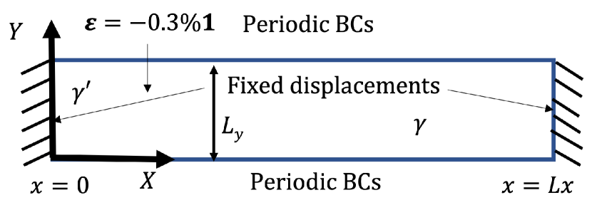
We first selected an elastically heterogeneous and isotropic Ni-Al alloy at K. The interface is assumed to be planar, and periodic boundary conditions have been enforced along the y-direction (Fig.1(a)). While the mechanical displacements () are fixed, and zero Neumann boundary conditions are enforced on the phase-field () and mole fraction variables along the x-direction. That is for all y and (see Table 3 & Fig. 1(a))
| (42) | ||||
| (43) | ||||
| (44) |
Here is the outward unit normal to the external surface and is the diffusion potential of Al. Although not apparent from Fig. 1(a), it bears emphasis that the longitudinal dimension in this simulation is 30 times that of the lateral dimension . Moreover, two scenarios have been considered: i) with a dilatational eigenstrain in the phase (case I); ii) no eigenstrains (case II). It should be emphasized that in case II, the transformation is driven solely by chemical driving forces. But in case I, both chemical (Eq. 35) and mechanical (Eq. 36) driving forces are present at the interface.
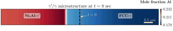
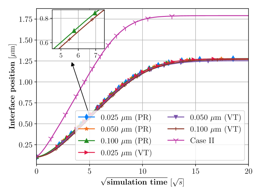
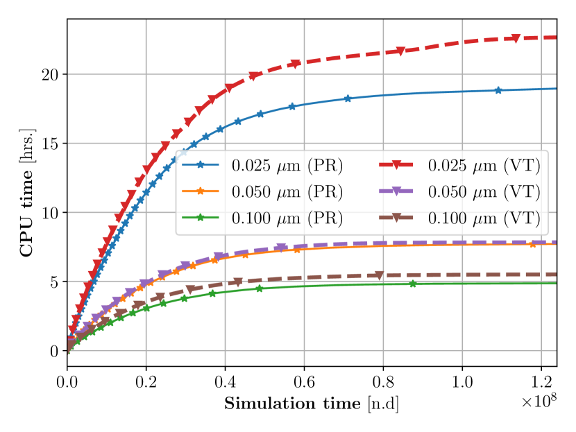
Our simulations show that the phase grows at the expense of phase with increasing time (Fig. 1(b)). For analysis, we focussed on the effect of two relevant model assumptions on simulation results: first is the choice of interface width, and second is the scheme of homogenization. For this reason, we compared the partial rank-one (PR) homogenization scheme with the Voigt-Taylor (VT) homogenization scheme for different interface width choices.
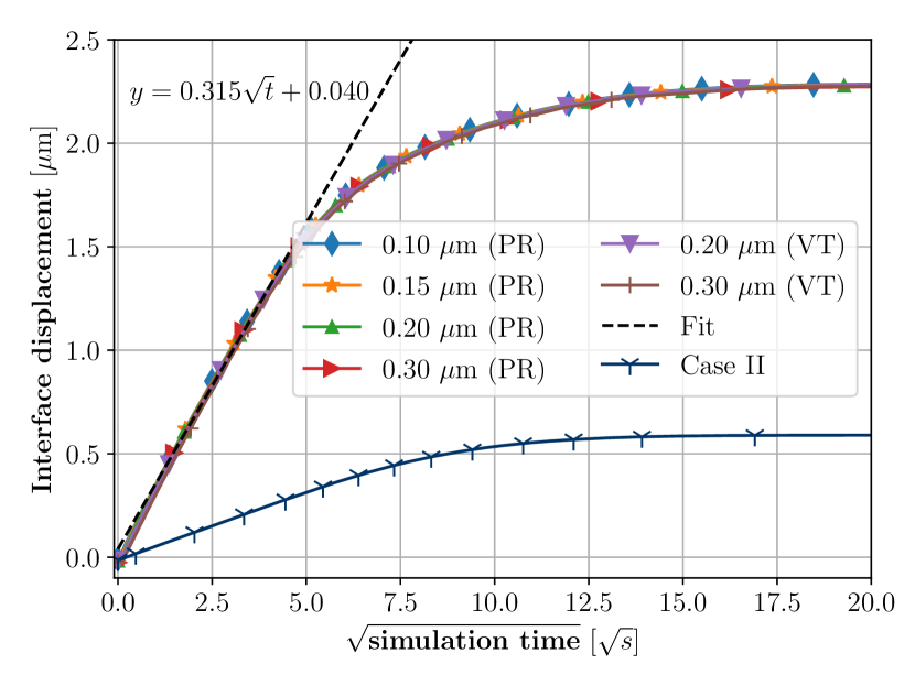
We find that the variation of interface position with time remains unaffected by our choice of interface width when simulated using both PR and VT schemes (Fig.1(c)). For case I, the phase follows a parabolic growth law for time s. As the system reaches towards the equilibrium state, the growth of the phase slows down. We also observe a parabolic growth behaviour for case II (Fig. 1(c)). However, we find that the coherent phase boundary grows much faster in case I as compared to case II.
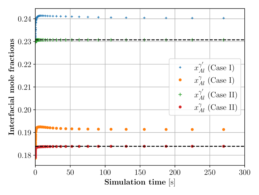
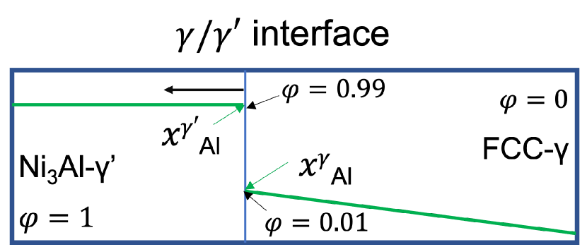
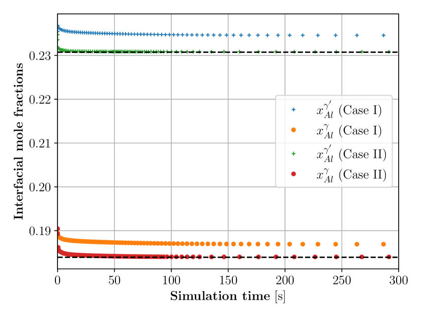
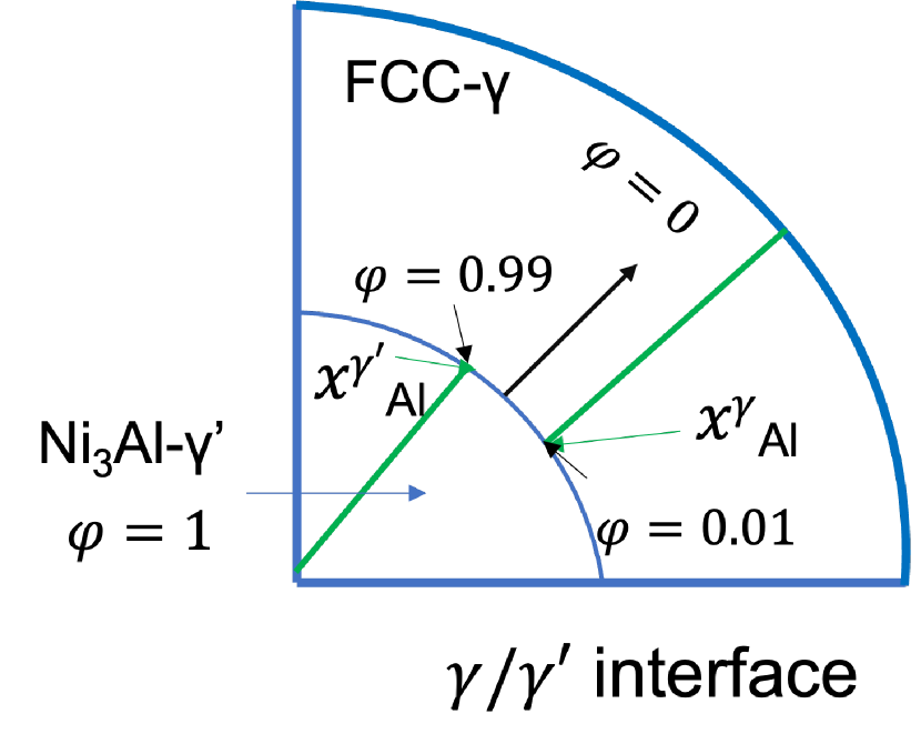
This behaviour can be attributed to the shift in local interfacial concentrations due to the presence of elastic fields. Johnson [81] analytically calculated this shift in the case of a sharp-interface model. To verify this, we track the temporal evolution of the Al mole fraction on the side of the interface by assigning the phase-field variable to be (Fig.2(b)). It is evident from Fig.2(a) that the interfacial concentrations in case II are higher compared to case I and are clearly due to the presence of elastic fields. Also, notice that the interfacial concentrations in case II deviate significantly from the equilibrium values (dotted line).
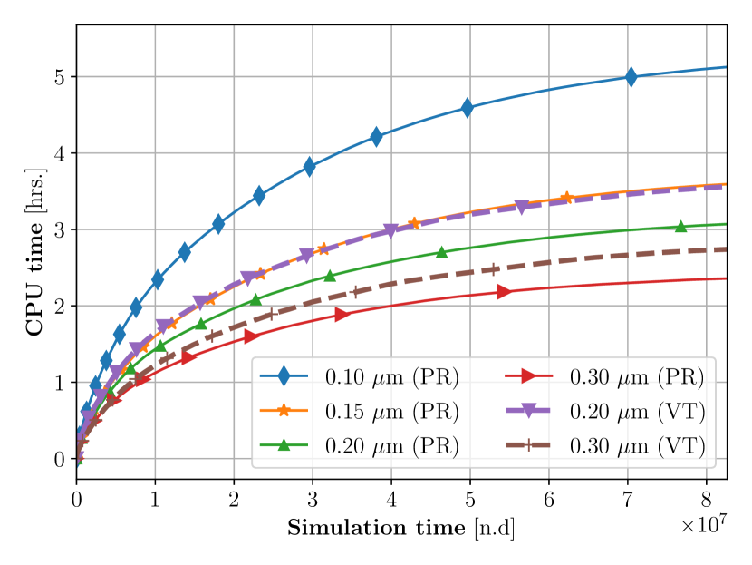
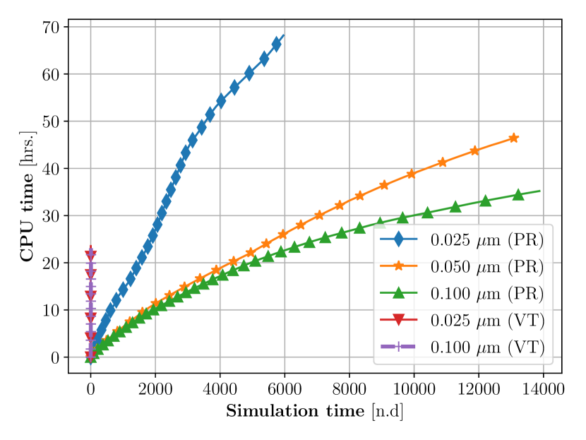
Interestingly, we also find that the PR scheme shows marginally better convergence than the VT scheme (Fig.1(d)). For a given value of simulation time and interface width, the PR scheme always outperforms the VT scheme in terms of CPU time (Fig.1(d)). Moreover, a trivial observation is that the CPU time decreases with increasing interface width (Fig.1(d)). This shows the advantage of controlling the interface width in a phase-field model without loss of simulation accuracy.
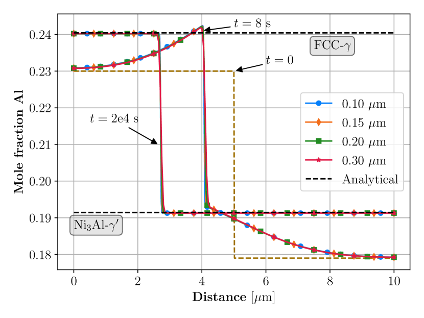
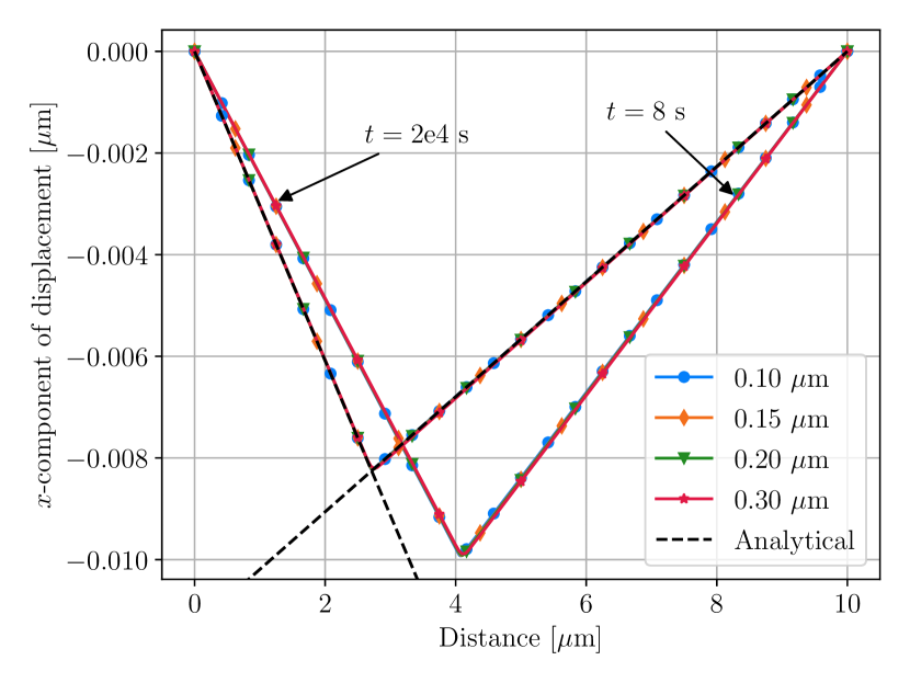
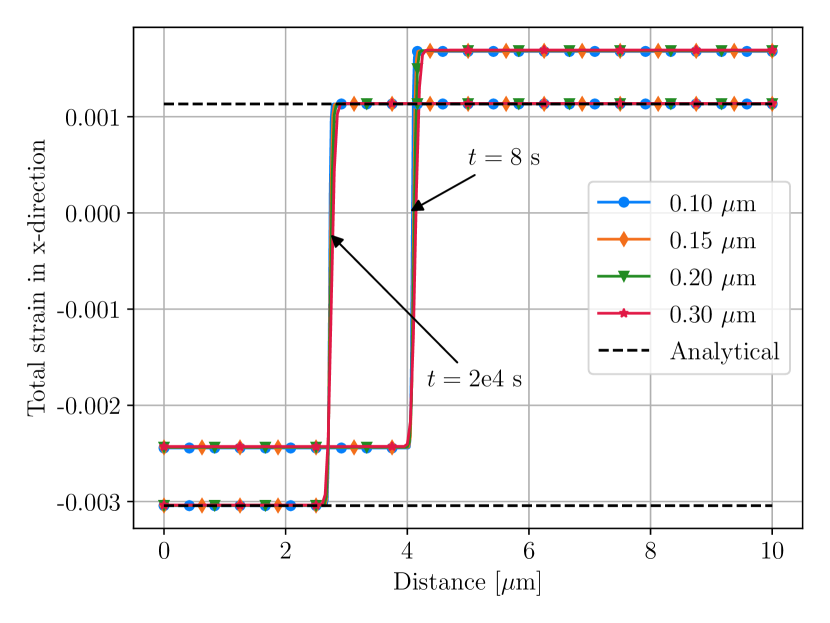
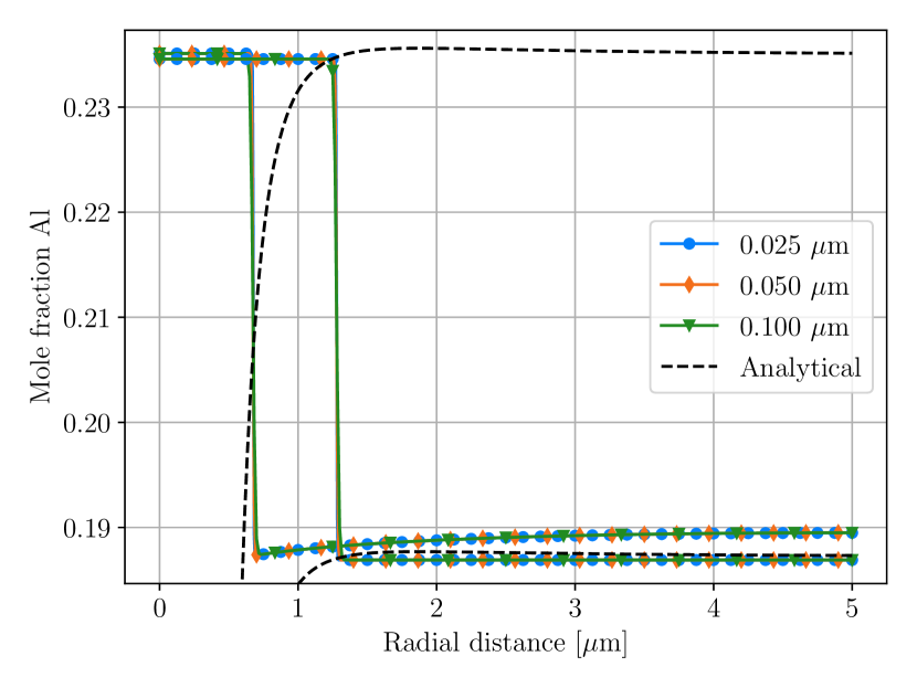
We then compared our simulated composition and elastic fields using the PR scheme with the analytically obtained elastic fields for the special case of plane stress (see Appendix D.1). To this end, we used the calculated interface position (Fig.1(c)) as an input in our analytical calculations, since the size of the inclusion is needed in the analytical result. Once the elastic fields were known, the interfacial equilibrium compositions were determined from the generalized Gibbs-Thomson equation (Appendix D). This comparison for different interface widths is shown in Fig.3. We find that the growth of phase is driven by the diffusion of Al from to (Fig.3(a)). Moreover, we find that the -component of the displacement field is maximum at the interface, and its slope decreases with increasing simulation time (Fig. 3(b)). This is reflected in the total strain field normal to the interface (Fig. 3(c)). It is also apparent that this strain is discontinuous at the interface. Due to the system geometry and boundary conditions, both the normal and the shear strains tangential to the interface are zero. Because of the eigenstrain, however, the tangential stress along the y-direction is non-zero and discontinuous (Fig.3(d)). These simulations also show that the calculated elastic fields are independent of interface width in this case.
3.2 Planar UO2-Vacancy simulation
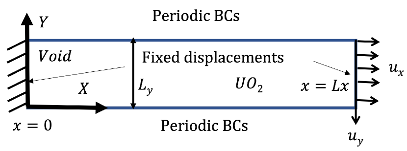
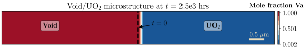
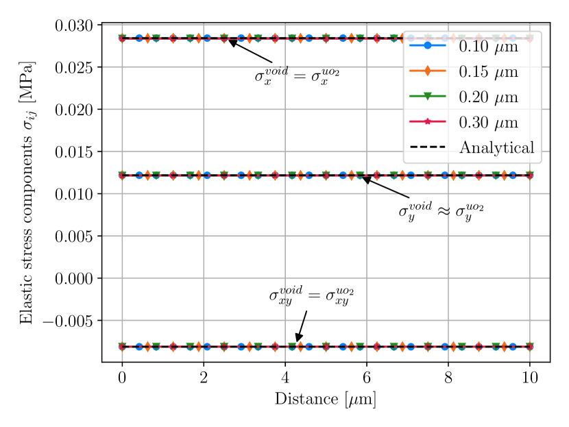
Next, we chose a UO2/void alloy where Young’s moduli show higher phase contrast compared to the Ni-Al case, but the system has no eigenstrains. Similar to the planar Ni-Al case, we have assumed periodic boundary conditions along the lateral direction. However, along the longitudinal direction, we have enforced the following Dirichlet boundary conditions on displacements (see Table 3 and Fig.4(a)):
| (45) | ||||
| (46) | ||||
| (47) |
Here nm is the characteristic length of the system, and are the x and y components of the displacement vector , respectively. Similar to our previous case, we have enforced zero Neumann boundary conditions on phase-field, and mole fraction variables (see Eqs. 43 & 44) along the left and right boundaries, and the longitudinal dimension is times that of the lateral dimension. It is also important to note that there are no eigenstrains in this system. Consequently, the elastic stresses are due to the imposed right boundary conditions on displacements.
Ideally, Young’s modulus of the void phase should be vanishingly small. We, however, assume the Young’s modulus of the void phase to be times the UO2 phase (see Table 2). This choice was based on two practical reasons. First, we referred to the work of Gururajan and Abinandanan [19]. Second, we found that for the non-planar case (discussed in section ), convergence to the equilibrium state was achieved only when the ratio of young’s moduli . Although for the planar cases, we found convergence even with a ratio of young’s moduli of the order of using the PR scheme.
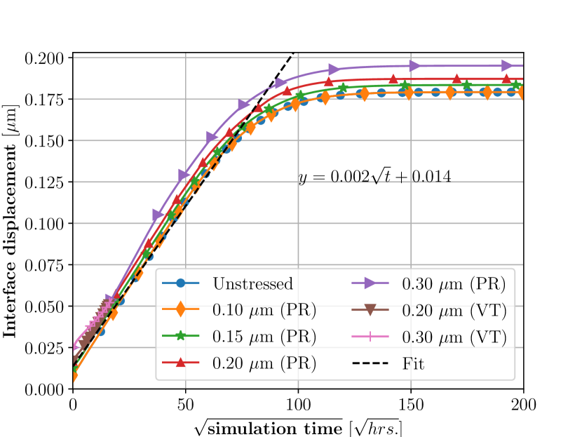
In contrast to the Ni-Al alloy, we find that the simulated interface displacement using the PR scheme depends slightly on the interface position in this alloy (Fig.4(c)). It is possible to explain this by measuring the strain jump normal to the interface. At the equilibrium state, our calculations show that the strain jump, in this case, is nearly times that of the case (compare Figs. 3(c) & 5(c)).
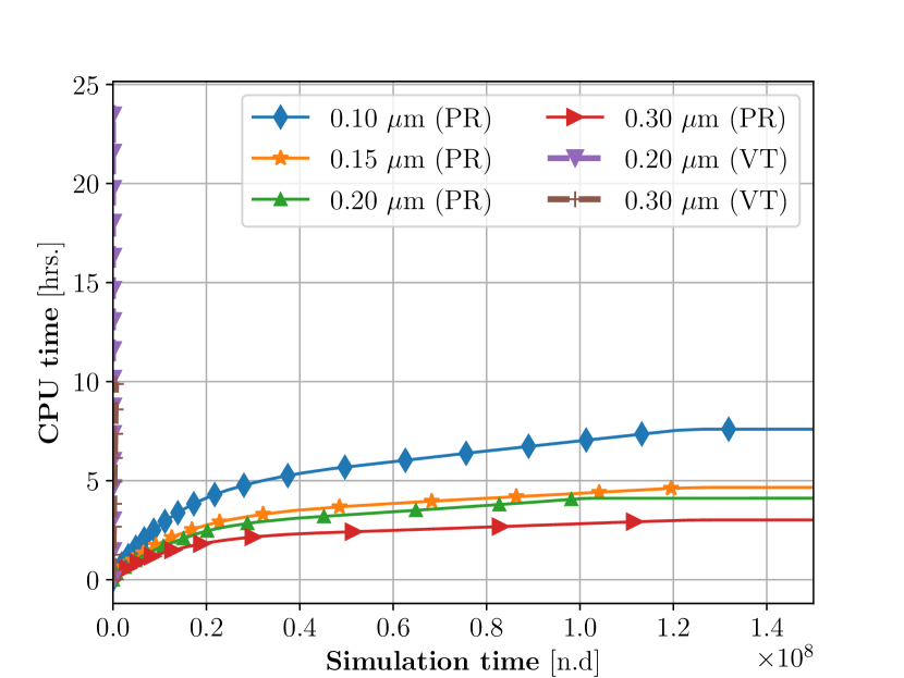
The reason is the high phase contrast with respect to elastic moduli. Specifically, the ratio of Young’s moduli, in this case, is nearly times that of the Ni-Al case (Table 2). Surprisingly, we find that this simulation was excruciatingly slow when the VT scheme was employed. Specifically, the interface migrated by m after a CPU time of 24 hrs with an interface width of m using the VT scheme (Fig.4(d)). On the other hand, this simulation was completed in less than hrs. using the PR scheme for the same interface width (Fig.4(d)). We observed similar results when a higher interface width was assumed. In our opinion, this is due to the difference in local driving force in the two schemes. This shows the advantage of the PR scheme over the VT scheme for systems exhibiting higher phase contrast with respect to Young’s moduli. Another contrasting observation compared to the Ni-Al case is that the interface position for case IV and case III does not differ significantly. The reason for this is the very low modulus of the void phase that leads to almost negligible stress within the system (Fig.5(d)).
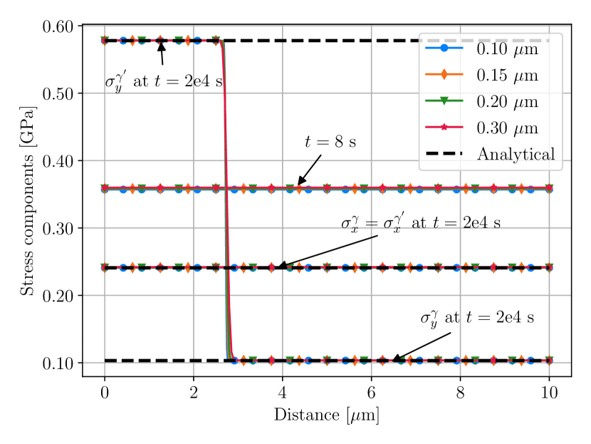
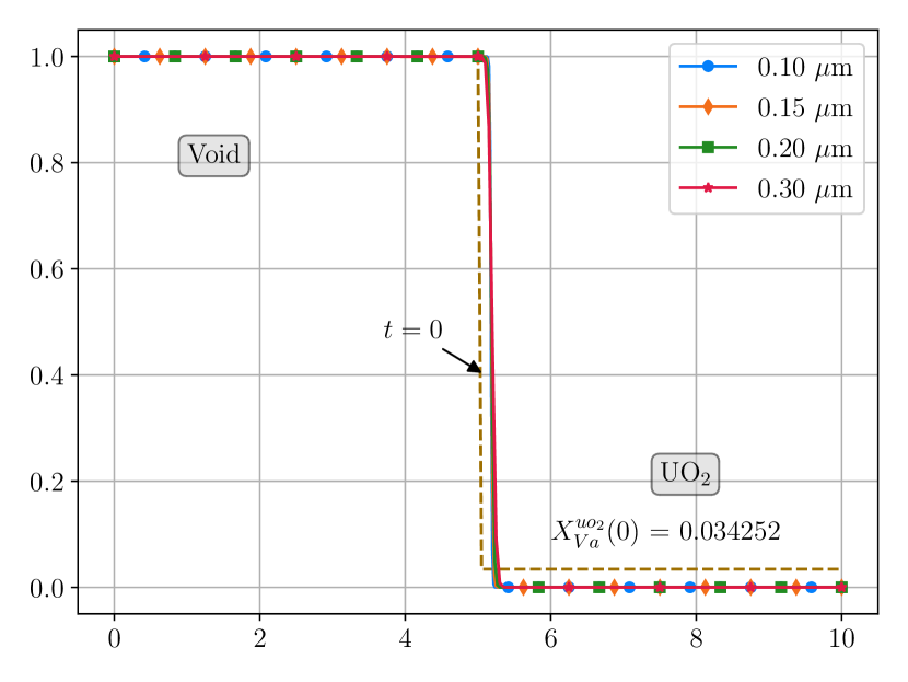
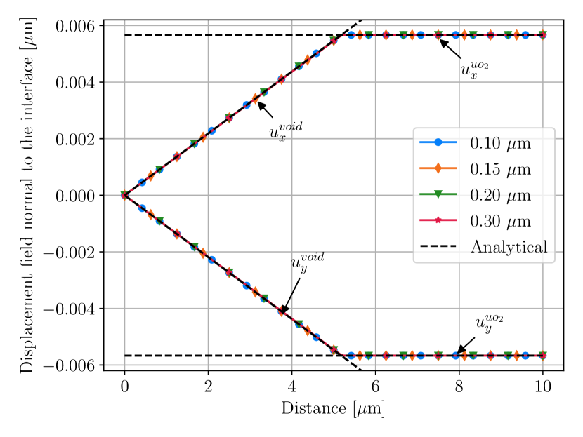
We then compared the simulated and the analytically calculated elastic fields for the special case of plane stress. We find that our simulated elastic fields show reasonable quantitative agreement with the analytical results (Fig.5). Since the net interface displacement, in this case, was very small ( m), we plotted the elastic fields only at the final time step. In direct contrast to the Ni-Al case, the displacement field in the y-direction is non-zero in this alloy (Fig.5(b)). This is due to the imposed downward displacement at the right boundary. Consequently, this mechanical displacement engenders shear strains within the system (Fig.5(c)), which are discontinuous at the interface. Note that, compared to the void phase, the deformation in the UO2 phase is negligible (Fig.5(c)). As mentioned before, due to the very low modulus of the void phase, the stresses within the system are negligible (Fig.5(d)). Nevertheless, we find that the quantitative accuracy of the simulated vacancy field and the elastic fields remain unaltered with changes in interface width.

3.3 Non-planar Ni-Al simulation
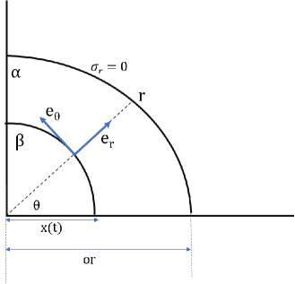
As a third example, we chose a Ni-Al alloy in which the phase boundary is non-planar. Specifically, we have considered a circular shaped precipitate embedded at the center of a circular shaped matrix. Due to the symmetry of the problem, we have simulated only a quarter of the domain. Moreover, zero Neumann boundary conditions have been assumed with respect to phase-field and mole fraction variables at all boundaries (see Eqs. 43 & 44). Further, symmetric boundary conditions have been imposed on displacements at the left and bottom boundaries, while the outer boundary is traction free (see Table 3 and Fig. 6(a)). This yields
| (48) | ||||
| (49) | ||||
| (50) |
Here is the stress and m is the outermost radius of the matrix. Again, we have considered two scenarios—with dilatational eigenstrains in the phase (case I) and without any eigenstrains (case II). It is noteworthy that we have performed these simulations in a Cartesian reference frame. For analysis, the simulated results were then transformed into polar coordinates for visualization and comparison with analytical results.
In contrast to our planar Ni-Al case, the initial conditions in this simulation are such that the phase grows at the expense of the phase. Due to system geometry and isotropic elastic properties, the simulated elastic fields are radially symmetric. To show this, the radial and tangential displacements are determined from the and displacements using
| (51) |
where . Here, and are the coordinates in the Cartesian frame. In Fig.6(b), we have plotted the radial displacement at time s. Moreover, we found that the tangential displacement is vanishing throughout the domain in this case.
Next, we focussed on the effect of interface width and the homogenization assumption on the simulation results. Our simulations show that the variation of interface position with increasing time is independent of the interface width choice when simulated using the partial rank-one homogenization scheme (Fig.6(c)). However, using the VT scheme, we find that this variation is slightly dependent on the interface width (see inset in Fig.6(c)). Moreover, we also find that the computation time to run the simulation using the PR scheme is always less than using the VT scheme (Fig.6(d)). It is interesting to observe that case I is kinetically slower compared to case II, which contrasts with the planar case during which the reverse was true. This is possibly due to the shift in the local equilibrium compositions at the interface due to the curvature driving force, as given by the generalized Gibbs-Thomson condition.
To verify this, we again determine the interfacial concentrations as a function of simulation time. Moreover, we follow the same procedure as described in the planar case to determine these concentrations. This is shown schematically in Fig. 7(b). In this case, we also find that the interfacial concentrations in case II are higher compared to case I (Fig. 7(a)). However, the magnitude of shift from the equilibrium values is lower in the non-planar case as compared to the planar case due to curvature effects.
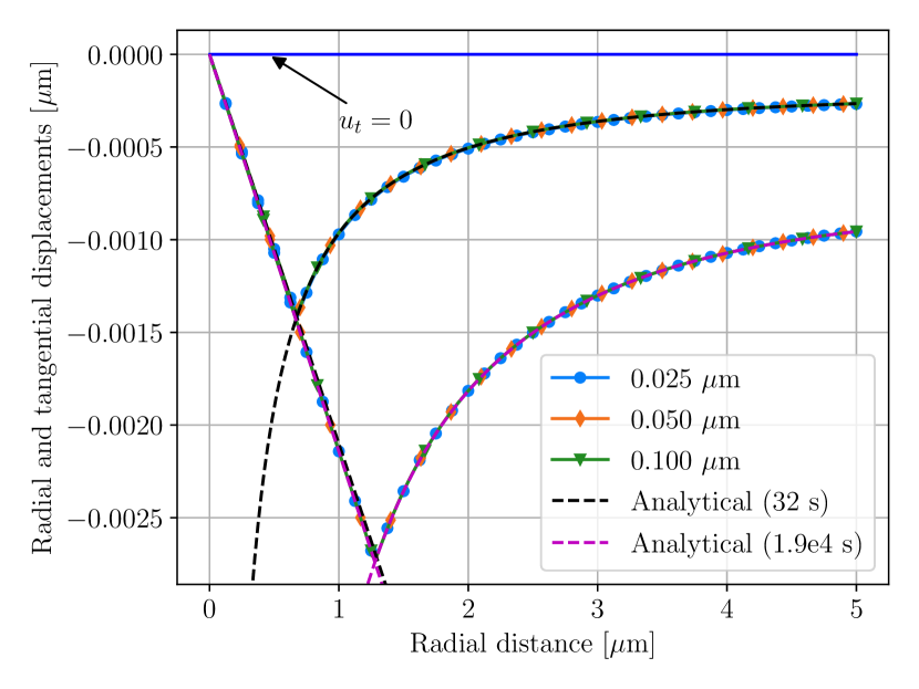
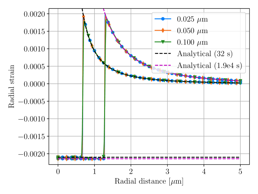
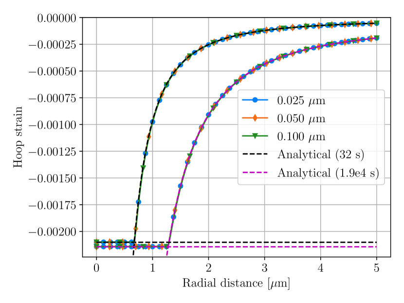
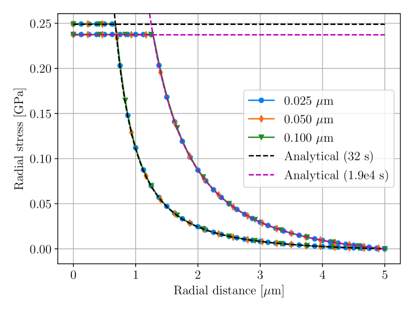
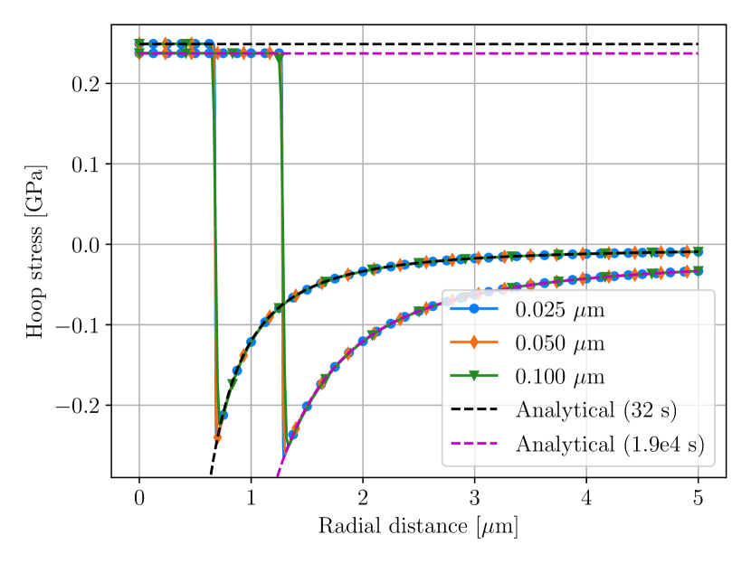
Moreover, we find that the simulated elastic fields (shown in polar coordinate frame) are in quantitative agreement with analytical solutions obtained assuming plane stress conditions (Fig.8). Fig.8(b) shows that the radial displacement field is maximum near the interface and increases with time. While the tangential displacement within both the precipitate and matrix phases is zero. Notice that the radial displacement field within the phase is linear as a function of radial distance. This indicates that both the radial and hoop strains are uniform within the precipitate phase with increasing growth (Figs.8(c) and 8(d)). However, in the matrix phase, the variation of radial and hoop strains with radial distance is non-linear. Consequently, the radial and hoop stresses are also uniform within the precipitate phase (Figs.8(c) and 8(d)). It is clear from this comparison that the simulated elastic fields using the partial rank-one homogenization scheme are independent of the interface width choice within the bulk phases but show slight deviations in the interfacial region.
3.4 Non-planar UO2-Vacancy simulation
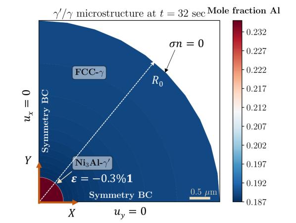
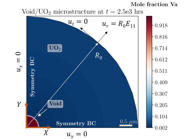
Next, we selected a non-planar UO2/void system. In this simulation, we have assumed a circular-shaped void embedded at the center of a circular-shaped UO2 matrix. Due to symmetry reasons, we have simulated only a quarter of the circular domain. Moreover, the boundary conditions on the phase-field and mole fraction variables are identical to the non-planar Ni-Al case. However, the boundary conditions on displacements are different at the outer-most boundary (see Table 3 and Fig. 9(a)). Specifically,
| (52) | ||||
| (53) |
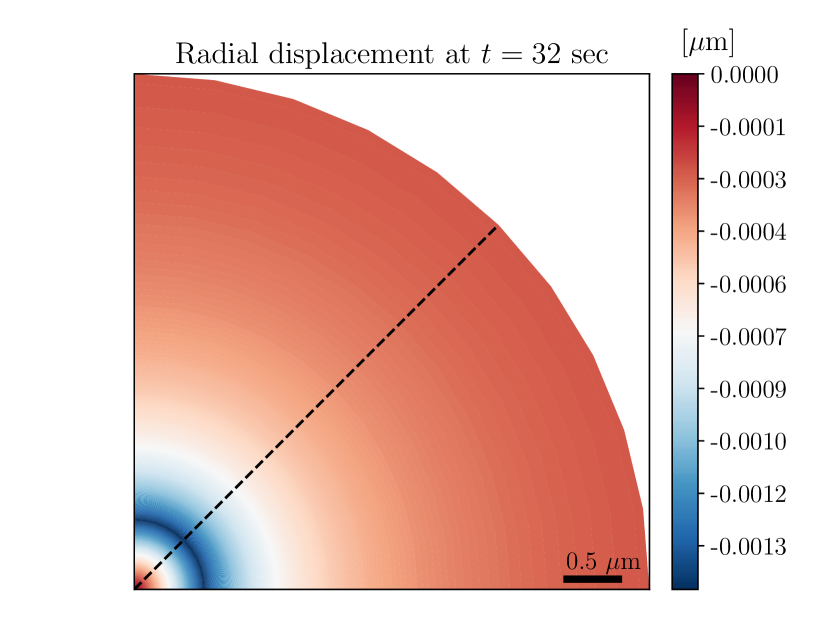
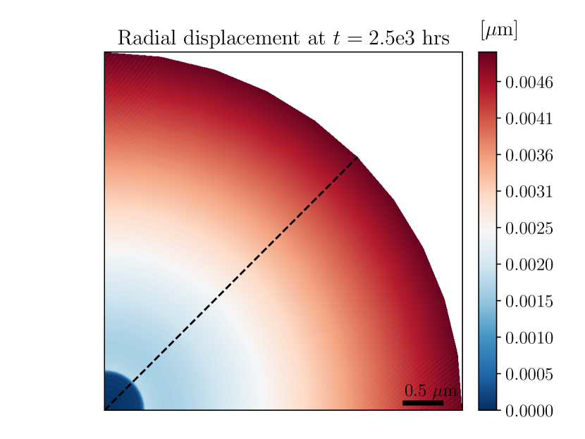
where for simplicity we have taken and m is the outermost radius of the UO2 matrix. As a consequence of this fixed boundary condition, it can be shown using Eq. (51) that the imposed tangential displacement is zero, but the radial displacement is equal to m at the outer boundary (see Figs. 9(a)-9(b)). Since the system has no imposed eigenstrains, the fixed boundary condition at the outermost boundary is the source of elastic stresses. Moreover, at the left and bottom boundaries, the displacement boundary conditions are identical to the non-planar Ni-Al case (Eqs. 48-49).
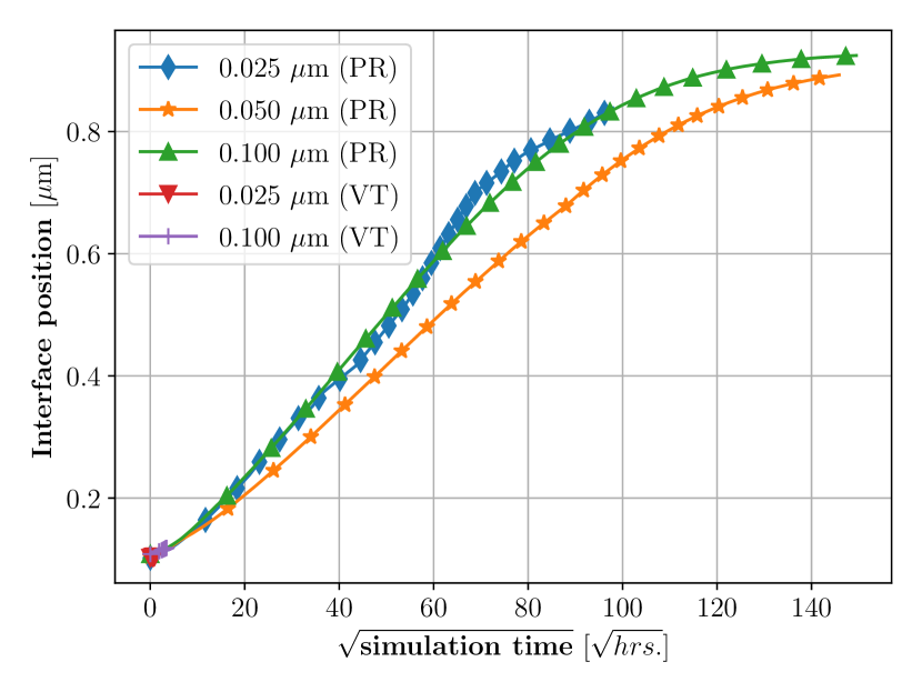
For the same interface width range as in the Ni-Al non-planar case, we find that the variation of interface position as a function of the square root of time depends on the interface width using the PR scheme (Fig.9(c)). Because of the strong elastic heterogeneity () this dependence on interface width is observed. However, similar to the planar UO2/void case, the VT scheme nearly fails to simulate the given alloy system (Fig.9(c)). This is mainly because the VT scheme has poor convergence compared to the PR scheme (Fig.9(d)). As mentioned before, this poor convergence is not due to our implementation since the governing equations remain the same but the thermodynamic driving force changes. To gain a quantitative understanding, we calculate the average time step, , that is, the ratio of total time by a number of time steps, for both schemes. Concretely, we find that the using the PR scheme is nearly times higher compared to the using the VT scheme for an interface width value of m.
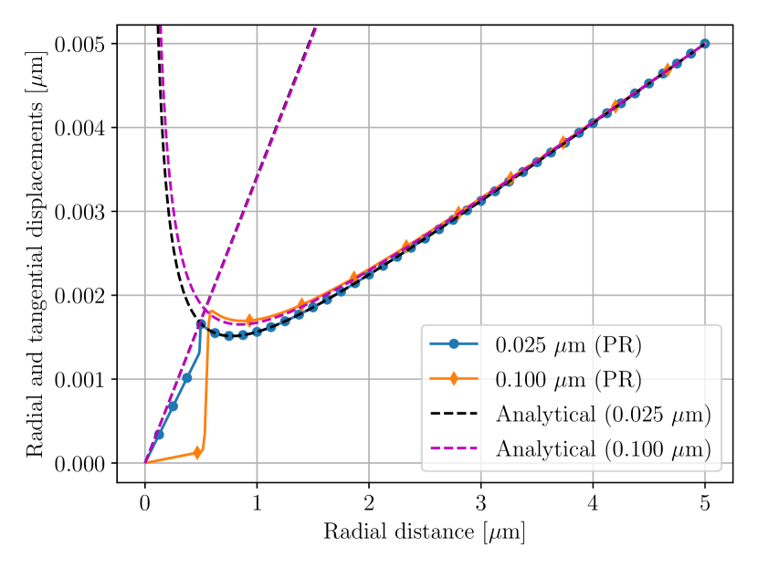
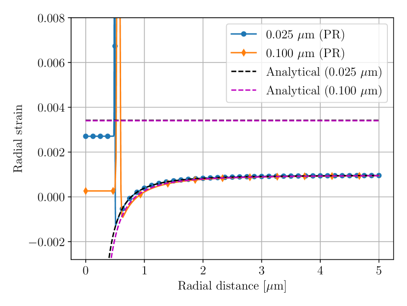
Also, in contrast to the planar UO2/void case, we find that the bulk elastic fields within the void phase depend on the interface position and deviate from the analytical solution (Fig.10). This analytical solution has been obtained assuming plane stress conditions. We find that the radial displacement field in the void phase is lower compared to the analytically predicted value for an interface width of m (Fig.10(a)). Moreover, the continuity of radial displacement is not satisfied near the interfacial region, in contrast to analytical predictions (Fig.10(a)). However, as the interface width is decreased to m, the simulated radial displacement field gets closer to the analytical solution (Fig.10(a)). Also, notice that the interface position slightly varies with a change in interface width, and thus the analytical solution in the UO2 phase shifts slightly near the interface. This trend is also reflected in the variation of radial strain as a function of distance (Fig.10(b)). Although the bulk radial strain is qualitatively similar to the analytical solution in the void phase, we find significant quantitative disagreement with the analytical solution for both interface widths. In the bulk UO2 phase, however, quantitative agreement between simulated and analytical solutions is obtained. We believe this is because of the extremely low modulus of the void phase compared to the UO2 phase. Nevertheless, this shows that for strongly heterogeneous alloys, the PR scheme should be preferred over the VT scheme, provided that the interface width value is taken to be less than (1/4) of the initial particle size.
3.5 Multiparticle simulation
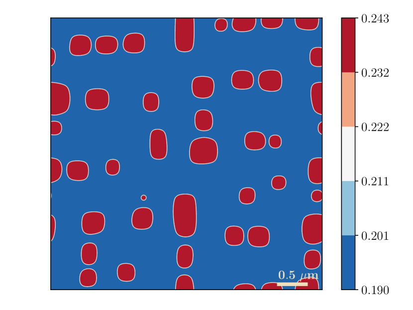
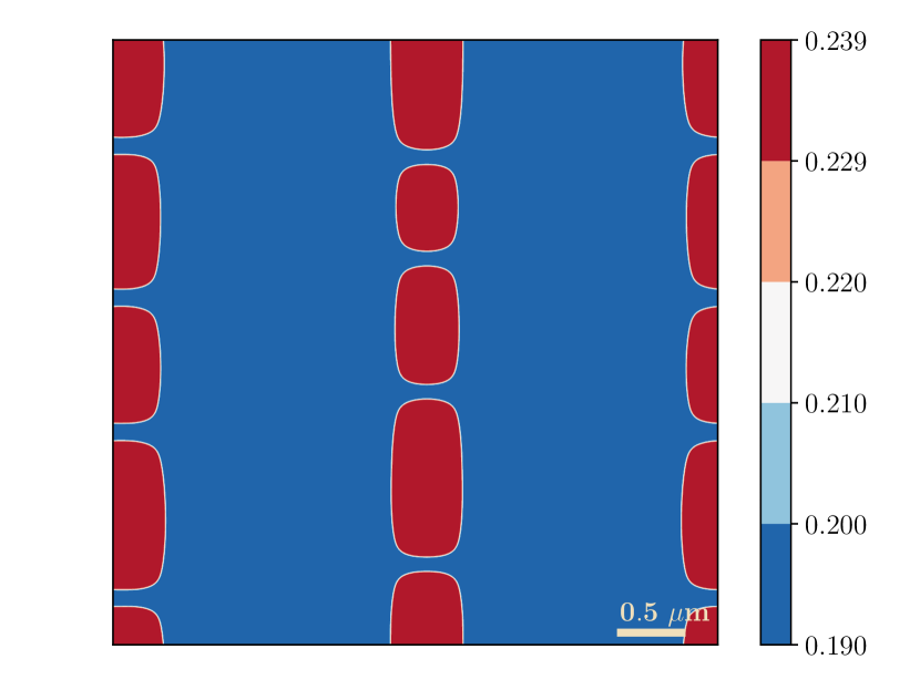
Finally, we simulated a multiparticle elastically heterogeneous and anisotropic system using the partial rank-one (PR) scheme. In this case, we have imposed periodic boundary conditions on all variables along both and directions. We initialize the system with a random distribution of 160 circular-shaped precipitates with a mean radius of m. An inbuilt adaptive mesh refinement capability within MOOSE was employed to reduce the computational costs of running simulations in a uniformly generated mesh.
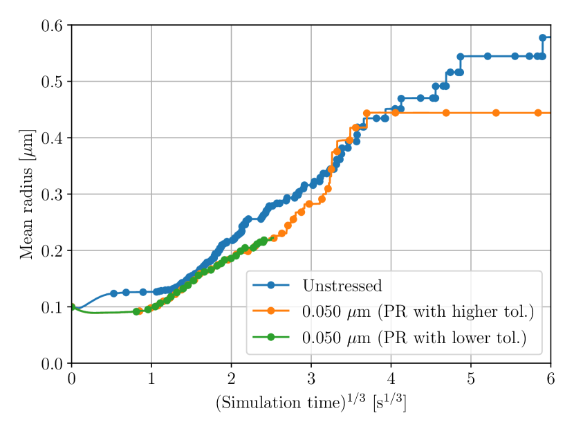
When the effect of elastic strain energy is small compared to the interfacial energy, the microstructure has a uniform distribution of precipitates (Fig.11(a)). However, with increasing time, we find that the precipitate shape becomes increasingly cuboidal (Figs. 11(b) and 11(c)). Moreover, the precipitates show preferential alignment along the elastically soft and directions. This preference is mainly due to the elastically anisotropic interactions between the precipitates. Moreover, the variation of the mean radius with the cube root of simulation time is shown in Fig.11(d). We find that the coarsening kinetics in case I is marginally slower compared to case II (Fig. 11(d)).
It must be pointed out that, with the exception of this simulation, we have used a relative non-linear tolerance of and an absolute non-linear tolerance of to obtain convergence in all four previous simulations. The reason for this is our simulation did not converge after time s when the tolerance values were set equal to the single-particle simulations (Fig. 11(d)). Therefore, we increased both these tolerances by a factor of . Consequently, the simulation converged to the equilibrium state (Fig. 11(d)). Moreover, a comparison of the coarsening kinetics shows that the accuracy of the simulation results remains unaffected despite this increase in tolerance values (Fig.11(d)).
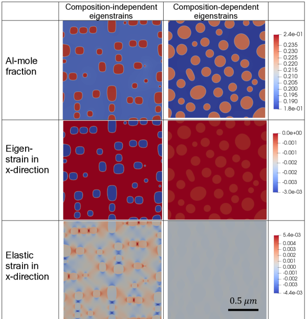
Lastly, to show the effect of composition on elastic fields, we have simulated the same multiparticle system by considering composition-dependent eigenstrains instead of constant eigenstrains. Since in a grand-potential model, the diffusion potential is the independent variable, this dependence arises indirectly through the phase compositions. Concretely, by assuming Vegard’s law [82], the eigenstrains in the phase can be written as
| (54) |
where , is the identity tensor, is the Al mole fraction of phase and is the overall Al mole fraction. For our case, this value was determined to be .
Fig.12 compares the simulated microstructures in both these cases at time s. Notice that as a consequence of Eq (54), the effective eigenstrains within the phases are much lower compared to the constant case (see the second row of Fig.12). For this reason, we find that the microstructure, in this case, is relatively more isotropic and randomly distributed compared to the previous case. Also, the elastic strains are negligible as compared to the constant eigenstrain case (Fig.12). It should be emphasized that despite coherency strains, the morphology, in this case, is isotropic. Moreover, this expected dependence of microstructure on the magnitude of eigenstrain has also been demonstrated experimentally for the case of Ni-Al-Mo alloy [83]. The possible dependence of compositions on elastic constants can be similarly modelled using Eq. (16). This demonstrates that our model can consider composition-dependent elastic properties through the phase compositions, and simulate its subsequent role in microstructure evolution.

4 Conclusions
In this work, we developed a two-phase multicomponent phase-field model for elastically heterogeneous two-phase solids based on a partial rank-one homogenization scheme. The uniqueness of this model is that both mechanical compatibilities and chemical equilibrium is ensured within the interfacial region. It was numerically solved using the fully parallelized MOOSE (Multiphysics Object-Oriented Simulation Environment) package. The current implementation is, therefore, capable of simulating elastically heterogeneous and anisotropic alloy systems. Its performance was demonstrated for two model binary systems— and UO2/void—at length scales much larger than the physical interface width.
We found that the partial rank-one homogenization (PR) scheme converged better compared to the Voigt-Taylor (VT) scheme for both the planar and the non-planar Ni-Al simulations. It was also found that using the former scheme, the variation of interface position with time was unaltered with increasing interface width in both these cases. However, when the latter scheme was employed, slight variation in interface position was observed with increasing interface width for the non-planar case. In both these cases, the simulated bulk elastic fields based on the PR scheme showed excellent quantitative agreement with analytical solutions at different time steps and were found to be independent of interface width choice.
We interestingly found that the PR scheme should be preferred over the VT scheme, particularly for the UO2/void simulations. This is mainly because of the extremely poor convergence of the VT-based simulations compared to the PR-based simulations for the same interface width range as in the alloy. We attribute this to the strong elastic heterogeneity in this system compared to the case. Precisely, the ratio of Young’s modulus of the particle to that of Young’s modulus of the matrix phase, in this case, was times higher than the Ni-Al case. Despite this strong heterogeneity, we found that the PR-based simulations reached the equilibrium state and showed good quantitative agreement with analytical solutions in the planar case. For the non-planar case, however, this quantitative agreement only holds true as long as the interface width is taken smaller than one quarter of the initial particle size.
Finally, we simulated the coarsening of precipitates in an elastically anisotropic Ni-Al alloy using the PR scheme. As expected in a coherently stressed system, the microstructure showed preferential alignment along the elastically soft directions. It was also observed that the coarsening kinetics was marginally slower in the stressed case compared to the unstressed case.
5 Acknowledgement
This work was supported by the European Research Council (ERC) under the European Union’s Horizon 2020 research and innovation program (INTERDIFFUSION, grant agreement no. ). The computational resources and services used in this work were provided by the VSC (Flemish Supercomputer Center), funded by the Research Foundation - Flanders (FWO) and the Flemish Government - department EWI. S.C thanks Dr. Michael Tonks at University of Florida, for allowing to use the supercomputer facility at University of Florida during the review process.
Appendix A
Derivation of jump vector and its derivatives
Here, we analytically derive expressions for the jump vector and its derivatives with respect to and for anisotropic two-phase solids. These derivates are then used to calculate the Jacobian terms in Appendices B and C.
To determine an expression for , we start by substituting Eq. (8) in Eq. (7) and use the minor symmetry of the stiffness tensor, i.e., to rewrite from Eq. (6). This yields
| (A.1) | ||||
Now, we solve for the unknown using Eq (A.1). Rearranging the known quantities on the left-hand side of Eq. (A.5) as a second-order tensor (denoted as ) yields
| (A.2) |
Substituting Eq. (A.2) in Eq. (A.1) and using yields
| (A.3) |
where denotes the inverse of tensor and . From Eq. (A.3) we note that depends on both the phase-field variable through the interpolation function in Eq.(A.2) and the total strain due to the jump in stiffness tensors. Consequently, it is useful to obtain these derivatives as well to calculate the Jacobian terms.
Thus, differentiating Eq. (A.3) with respect to , using the identity , the minor and major symmetries of stiffness tensors, i.e., and , yields
| (A.4) |
Next, to calculate , we take the implicit derivative of Eq. (A.1) after using the expression for . This gives
| (A.5) |
The inverse of is given in Eq. (A.2) and its derivative with respect to is calculated by differentiating Eq. (A.2) to obtain
| (A.6) |
Eqs. (A.3), (A.4) and (A.5) are the main results of this appendix.
Appendix B
Derivation of stress and its derivatives
In order to derive the overall stress , we first note that the derivative of Eqs. (4) and (5) with respect to total strain may be written as:
| (B.1) | ||||
| (B.2) |
Then, differentiating Eq. (13) with respect to total strain yields
| (B.3) |
Using the definition , symmetry of stress tensor, i.e. and substituting Eqs. (B.1) and (B.2) in Eq. (B.3) yields
| (B.4) |
Moreover, from Eq. (6) we see that
| (B.5) |
Again by using the symmetry of stress tensor it is easy to show that:
| (B.6) |
By substituting Eq. (B.6) in Eq. (B.4) yields
| (B.7) |
Because of Eq. (7) we find that the last term in Eq. (B.7) must be zero. Thus, we can simplify Eq. (B.7) to
| (B.8) |
Eq.(B.8) was also given by Kiefer et al. [66], with the difference that replaces . Moreover, for numerical implementation, the derivatives of Eq. (B.7) with respect to total strain and the phase-field variable are needed. To this end, we differentiate Eq.(B.7) and denote by
| (B.9) | ||||
Because of Eq. (A.4) we must note that the second derivative of the magnitude of strain jump is zero, i.e. .
Now, by using the definition , minor symmetry of stiffness tensors, i.e., and substituting Eqs. (B.1) and (B.2) in Eq. (B.9) yields
| (B.10) |
All quantities on the right-hand side of Eq. (B.10) are known. An expression for has been obtained in Appendix A. To obtain , differentiate Eq. (6) with respect to total strain . This yields
| (B.11) |
Due to the minor symmetry of stiffness tensors and using Eq.(B.11), it can be shown that the second term in Eq.(B.10) may be written as:
| (B.12) |
Next, we want to calculate the derivative of Eq.(B.7) with respect to the phase-field variable . To this end, we first differentiate Eqs. (4) and (5) with respect to . This gives
| (B.13) | ||||
| (B.14) |
Differentiating Eq. (B.7) with respect to and denoting yields
| (B.15) | ||||
In the above equation, we note that we have omitted all terms that included the term , since this quantity is zero, as mentioned before. Finally, substituting Eqs (B.13) and (B.14) in Eq. (B.15) we obtain
| (B.16) | ||||
Eqs. (B.8), (B.10) and (B.16) are the main results of this appendix.
Appendix C
Derivation of driving force and its derivatives
In order to derive the driving force, we first differentiate Eq. (11) with respect to the phase-field variable . This gives
| (C.1) |
Substituting Eqs. (B.13) and (B.14) in Eq. (C.1) yields
| (C.2) | ||||
Moreover, by differentiating Eq. (6) with respect to we obtain
| (C.3) |
By substituting Eq.(C.3) in Eq. (C.2) and using the symmetry of stress tensor, i.e., yields
| (C.4) | ||||
Because of Eq.(7) we see that the last term in Eq.(C.4) must be zero. Consequently, Eq.(C.4) may be rewritten as
| (C.5) |
where we have denoted . It must be pointed out that this equation is consistent with that given by Kiefer et al. [66] (see Eq. (33)), provided the chemical contribution is ignored and is replaced with . One can also show that, without the chemical contribution, Eq. (C.5) is of the exact form as the “driving traction” derived by Abeyaratne and Knowles [84] in a sharp-interface setting. With the chemical contribution, Eq. (C.5) was given by Larche and Cahn [76] for a planar interface and by Johnson and Alexander [85] for a curved interface in a sharp-interface setting.
Furthermore, for numerical implementation we also require the derivative of Eq.(C.4) with respect to total strain. Thus, differentiating Eq. (C.4)
| (C.6) | ||||
By substituting Eqs. (B.1) and (B.2) in Eq. (C.6) yields
| (C.7) | ||||
Moreover, by first multiplying Eq. (7) with , then differentiating it with respect to total strain , and using Eqs. (B.1)-(B.2) gives
| (C.8) |
Because of Eq. (C.8) we see that the sum of last two terms in Eq.(C.7) must be zero. Consequently, Eq.(C.7) may be simplified to
| (C.9) | ||||
Appendix D
Analytical solutions
In order to analytically solve the equations of mechanical equilibrium in any coordinate system, the position of the interface at any instant , i.e., , must be given. In our validation results, we first perform a phase-field simulation for a given set of initial conditions and then use the numerically determined interface position at a given instant while comparing the analytical solution with the simulated solution. The interface position is numerically obtained by tracking the phase-field variable . Therefore, we do not make any a priori assumption about the inclusion size.
D.1 Solution for a flat interface
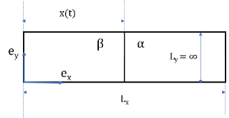
Consider a rectangular domain with a flat interface separating the and phases. We further assume that the y-dimension is much greater than the x-dimension, which is finite and ranges from . Therefore, we enforce periodic boundary conditions along the y-direction and Dirichlet boundary conditions with respect to the displacement fields. For sake of simplicity, let only the x-component of displacement fields, i.e., and , be non-zero at the left and right boundaries. Then, the x-component of the displacement field will be non-zero. That is
| (D.1) |
It immediately follows that the total phase strain in phase is given by . Since the phase has a non-zero eigenstrain , the non-zero stress components are
| (D.2) | ||||
| (D.3) |
Moreover, the equation of mechanical equilibrium simplifies to
| (D.4) |
where indicates the phase. Substituting Eqs. (D.2) in Eq. (D.4) yields
| (D.5) |
For this reason, the x-component of the displacement field must be linear within each phase
| (D.6) |
where , , , are the undetermined constants. From Eq.(D.6) and using the boundary conditions yields
| (D.7) | ||||
| (D.8) |
Now, since the displacement field must be continuous at , i.e., . From Eqs. (D.6), (D.7) and (D.8) we have
| (D.9) |
Rearranging Eq. (D.9) yields
| (D.10) |
Furthermore, the stress component normal to the interface plane must be continuous, i.e., . This yields
| (D.11) |
Substituting Eq. (D.10) in Eq. (D.11) and solving for yields
| (D.12) |
For the UO2/void case, since we have enforced a displacement along the y-direction, the y-component of the displacement field and the shear strain are non-zero in this case. We also assume that the y-component of the displacement field is linear in both phases. Then,
| (D.13) |
where , , , are the undetermined constants. From Eq. (D.13) and using the boundary conditions yields
| (D.14) | ||||
| (D.15) |
where and are the y-components of the displacement field at the left and right boundaries. Similar to the above-mentioned derivation, by enforcing the equality of the y-component of the displacement field and solving for yields
| (D.16) |
Now, since the shear components of the stress tensor must also be equal, i.e. . Using Eq. (D.16) and solving for this equality yields
| (D.17) |
D.2 Solution for a heterogeneous inclusion subject to zero radial stress at the outer boundary
We assume that the displacement field is dependent on the radial direction only within each phase and is of the form . Then the strain-displacement relations in polar coordinates for a given phase, say , can be written as
| (D.18) | ||||
For the simplicity’s sake, we first assume an elastically homogeneous and isotropic two-phase system. Then, the stress-strain relations take the following simple form
| (D.19) | ||||
Note that for the inhomogeneous case, the Lame’s parameters, and , will be denoted with a superscript indicating the stress state within that phase. Since the elastic stresses depend on the radial position only, the equation of mechanical equilibrium then reduces to
| (D.20) |
Substituting Eqs. (D.18) & (D.19) in Eq. (D.20) yields
| (D.21) |
From Eq.(D.21) we see that takes the following general form
| (D.22) |
where , , and are the undetermined constants. Since the radial displacement must be bounded, therefore must be zero when . To model finite domains, we assume that the radial stress at the outer radius is zero.
| (D.23) |
Using Eqs. (D.22) and (D.19) in Eq. (D.23) we see that
| (D.24) |
For an inhomogeneous inclusion, it can be shown that . Moreover, since the radial displacement field must be continuous at . Using Eqs. (D.22) and (D.24) yields
| (D.25) |
For an inhomogeneous inclusion, it can be shown that . Since the radial stress must be continuous, using Eq. (D.19), we see that
| (D.26) |
Using Eqs. (D.18), (D.22), (D.24) and (D.25) in Eq. (D.26) and solving for yields
| (D.27) |
Using expressions for and for the inhomogeneous case, it can be shown that for an inhomogeneous inclusion, is equal to
| (D.28) |
In summary, the elastic quantities for the homogeneous case within each phase can be written as:
| (D.29) |
| (D.30) | ||||
| (D.31) |
| (D.32) | ||||
| (D.33) |
For the inhomogeneous case, we have
| (D.34) |
| (D.35) | ||||
| (D.36) |
| (D.37) | ||||
| (D.38) |
D.3 Solution for an elastically heterogeneous system subject to radial strain at the outer boundary
The radial displacement field within both phases, say and , must satisfy Eq.(D.22). Following similar arguments, as discussed in the previous case, the value of must be zero; for the radial displacement field to be finite. Consequently, for this problem, the radial displacement field takes the following form:
| (D.39) |
Since the radial strain at the outer boundary is specified, say , then using Eq.(D.18), it follows that
| (D.40) |
Substituting Eq. (D.40) in Eq. (D.39) and enforcing the continuity of radial displacement at the interface yields
| (D.41) |
Now, by using the inhomogeneous form of Eq. (D.19) and solving for the equality of radial stresses at the interface yields
| (D.42) |
Substituting Eqs. (D.40) and (D.41) in Eq.(D.42) and solving for yields
| (D.43) |
Thus by substituting , , and in Eq. (D.39) yields the radial displacement for this case.
D.4 Solute mole fractions in an elastically stressed solid
To calculate the equilibrium mole fractions, and , in a stressed two-phase binary alloy, a set of two equations is required. The first equation represents the local thermodynamic driving force of the transformation, and the second equation is due to the assumption of local thermodynamic equilibrium at the interface. Specifically,
| (D.44) | ||||
| (D.45) |
By solving coupled Eqs. (D.44) and (D.45), and can be determined. It must be noted that this solution requires that the stress and strain in the bulk phases are known. From Eq. (D.45), we see that . Consequently, by Taylor expansion about the unstressed equilibrium diffusion potential, i.e. , the grand-potentials of a phase can be written as:
| (D.46) |
Substituting Eq. (D.46) in Eq. (D.44), and using the relations and , Eq. (D.44) can be rewritten as:
| (D.47) |
This equation represents the deviation of the unstressed equilibrium diffusion potential from the stressed case. Following this, the equilibrium mole fraction in the stressed solid can be easily obtained by Taylor approximating the mole fractions about the unstressed equilibrium mole fractions:
| (D.48) | |||
| (D.49) |
where represents the inverse of a thermodynamic factor of component B in phase .
Appendix E
Method to calculate diffusion potential
Diffusion potential is calculated numerically by solving Eq. (26) in the MOOSE (Multiphysics Object-Oriented Simulation Environment) framework [74]. Specifically, this equation is implemented as a MOOSE Kernel [74]. In this section, we discuss how this Kernel is implemented, and also provide a link to the source code.
To write a Kernel, two terms are needed: a residual vector and a Jacobian matrix [74]. Further, the residual vector is obtained by first deriving the weak form [74]. Specifically, for an independent diffusing component , the weak form of Eq. (26) is
| (E.1) |
where is the volume of the domain; is a suitable test function; is the interpolation function; are the phase mole fractions of and phases; and is the overall mole fraction. It should be emphasized that and are prerequisite input properties that are needed as functions of diffusion potentials. Moreover, these properties can be calculated either analytically [37] or numerically [69] depending on the solution model. Hence, these properties are implemented as Material objects in MOOSE [74]. On the other hand, is a field that has to be determined by solving the composition evolution Eq. (28).
Subsequently, we discretize Eq. (E.1) using the Galerkin finite element method [74]. It can be shown that the component of the residual vector associated with this Kernel is
| (E.2) |
where is the shape function at the node and , & are the discretized field variables such that
| (E.3) |
Here, is the total number of nodes in an element, and are the nodal values of diffusion potential and phase-field variables at node , and is the nodal value of mole fraction variable of component at node . Now, in order to iteratively solve Eq.(E.2), the Jacobian matrix has to be derived.
Notice that the residual vector is a function of , & , and consequently three derivatives are needed to construct the Jacobian matrix. First, the components of the Jacobian matrix associated with the variable are
| (E.4) |
where is the nodal value of the diffusion potential variable of the chemical component at node and are the components of the susceptibility matrix [37]. This matrix can be calculated by inverting the thermodynamic factor matrix [69], and is implemented as a MOOSE Material object. Second, the components of the Jacobian matrix associated with the variable are
| (E.5) |
where is the first derivative of the interpolation function .
Lastly, we take the derivative of Eq. (E.2) with respect to the nodal values . This yields
| (E.6) |
By implementing Eqs. (E.2), (E.4), (E.5) and (E.6) we can obtain the diffusion potential of a component . For a binary alloy, it is implemented as a C++ object: BinaryPhaseConstraintMu.C. This code is publicly available at https://github.com/souravmat-git/gibbs.
It should be noted that so far we have tacitly assumed that the eigenstrains and elastic modulus are constants. Consequently, the supplied phase mole fractions are not explicitly dependent on the elastic fields within the bulk phases (see Eq.16). This however does not imply that the diffusion potential, and consequently the phase mole fractions, are independent of elastic fields. The phase compositions at the interface are still dependent on the elastic fields, and consequently on the interface position. More concretely, in case of a sharp interface model, this dependence was analytically shown by Johnson [81] (see Eq. 17). As a result of this dependence, the growth velocity depends on the elastic fields [81].
However, for cases when the eigenstrains and elastic modulus are dependent on composition, there is an explicit dependence of phase mole fractions on elastic fields within the bulk phases. As an example, for a binary A-B alloy to model only composition-dependent eigenstrains, using Eq. (18) we obtain
| (E.7) |
Note that as a result of the second term there is a now a dependence of phase compositions on elastic fields even within the bulk phases. Since it is difficult to determine the dependence of eigenstrains on diffusion potentials, we can use chain rule to write
| (E.8) |
where is the solute susceptibility of phase . Assuming a first order Taylor dependence of eigenstrains on composition [82], we obtain
| (E.9) |
where is the overall (or average) alloy mole fraction. Eq. (E.9) indicates that the eigenstrains are dependent on the the local compositions within the bulk phases. Moreover, Eqs. (E.7), (E.8) and (E.9) are implemented as Material objects namely: StrainDependentTaylorApproximation.C, EigenStrainPhaseMaterial.C and EigenStrainPrefactor.C, respectively, and are freely available at https://github.com/souravmat-git/gibbs.
Appendix F
Discussion on the non-variational term
For a discussion on the role of non-variational term in case of the partial rank-one homogenization scheme, we have divided this appendix into two sections. First, we show the influence of the variational term on simulation accuracy for three of the considered simulations. We also show that in one of the simulations the inclusion of this term leads to a non-converging solution. Following this, we discuss possible reasons for this non-convergence.
F.1 Problem
To understand the effect of the variational term on simulation accuracy, we repeated the non-planar single particle simulation with an interface width of m with the variational term. Fig.1(a) shows that the presence of this term has no effect on the variation of interface position as a function of square root of time. We further note that this behaviour was also observed in case of the planar Ni-Al simulation. However, for the case of non-planar single particle UO2/void simulation having an interface width of m, we found that due to the presence of the variational term the simulations were not converging. Fig.1(c) shows that, although the simulation accuracy remains unaffected, the run time in the presence of variational term is significantly lower compared to the simulation without this term. Moreover, the computation time is approximately timer higher in the presence of the variational term compared to the simulation without this term (Fig.1(d)). Contrastingly, for the planar UO2/void case with the same ratio of Young’s moduli, we found that this term had no influence on simulation accuracy for the same interface width value m (Fig.1(e)).
The reason for the increase in computation time, in case of non-planar UO2/void simulation with the variational term, is the concurrent effect of increase in the number of non-linear iterations (Fig.2(a)) and the decrease in time step size (Fig.2(b)), as compared to the simulation without this term. Nevertheless, it is noteworthy that there was no speed-up in terms of computation time (Fig.1(b)) and time step size (Fig.1(f)) due to the exclusion of this term in case of non-planar Ni-Al and planar UO2/Va cases, respectively. Next, we attempt to explain this poor convergence for the case of non-planar UO2/void simulation with the variational term.
F.2 Reason
For sake of discussion, we note that the variational term is the divergence of a vector quantity, , which has dimensions of J/m2. So in order to determine the influence of the variational term, we look at the magnitude of this vector quantity. Since this quantity is temporally and spatially dependent, we calculate its local and average values. For our simulations, we define the average value of a quantity, , as
| (F.1) |
Additionally, since we employ non-dimensional quantities, the vector term can be written in non-dimensional form as
| (F.2) |
where [J/m3] is a characteristic modulus used to non-dimensionalize the stresses and [J/m3] is the barrier height. Note that indicates non-dimensional values. As discussed in the text, we have taken to be the shear modulus of the precipitate and UO2 matrix in the Ni-Al and UO2/vacancy simulations, respectively. Further, it can be shown that
| (F.3) |
where is the norm of . By substituting Eq. (F.3) in Eq.(F.2) we can rewrite the total vector term as a vector sum of two vectors, and , such that
| (F.4) |
where
| (F.5) | ||||
| (F.6) |
It is important to note that due to the factor , the vector terms in Eqs. (F.4) (F.5) & (F.6) are non-zero only in the interfacial regions. Moreover, since we have defined the unit normal to the interface as , and by employing PRH scheme static compatibility at the interface is ensured, we have
| (F.7) |
As a consequence of Eq. (F.7), we note that the vector term in Eq.(F.6) must be vanishingly small. To test this, we determined the average value of the magnitude of these vectors, i.e., Eqs. (F.4) (F.5) & (F.6), using Eq.(F.1).
We find that the average value of the magnitude of is vanishingly small for both and UO2/void simulations (Figs. 3(b) and 4(b)). This implies that is nearly equal to . This is also evident from Figs. (3(a)) and (4(a)) in the case of and UO2/void simulations. Moreover, it is important to observe that the magnitude of is at least six orders of magnitude higher in case of UO2/void compared to simulation. Since in both cases, we can neglect in our analysis.
Now, since is directly proportional to the strain jump vector , we determined its local and average value in both cases. Figs. 4(a) and 4(b) show the local variation in the jump magnitude,, for the case of and UO2/void simulations, respectively. We find that the jump magnitude in the UO2/void case (see Fig. 4(b)) is nearly 300 times higher compared to the case (see Fig. 4(a)). This is due to the high phase contrast in the former case as compared to the latter. Moreover, it is due to this high magnitude of that the presence of the variational term leads to a non-convergent solution. For this particular case, it is therefore difficult to exactly ascertain its effect on simulation accuracy for longer computation time. Nevertheless, despite having the same ratio of Young’s moduli, in case of the planar UO2/void simulation this term has no effect on solution accuracy (Fig.1(e)). This can again explained by calculating the strain jump magnitude . We find that the strain jump magnitude in the planar case is at least four orders of magnitude lower compared to the non-planar UO2/void case (compare Figs. 4(c) & 4(b)). This value is lower in the planar case possibly because the strain jump vector depends on both the difference in Young’s moduli between the phases and the total strain at the interface (Eq. 9).
Moreover, it should be emphasized that the driving force due to bulk contributions, , consists of two terms in case of the partial rank-one scheme: the non-variational term and the variational contribution (Eq. 22 in the revised manuscript). Although not shown here, we found that the vector term was significantly lower in case of Ni-Al simulations compared to the non-variational term. Therefore, the variational term had no effect on the accuracy of the solution, and the interface was driven solely by the non-variational term. Contrastingly, this term was not insignificant compared to the non-variational term for the case of UO2/void. We think because of the high magnitude of this term relative to the non-variation term the simulations were not converging. It is worth noting that “thin-interface” phase-field models where a relation between model parameters and interfacial quantities can be obtained are particularly suited when the driving forces due to bulk contributions are small [43]. It also partially explains why in case of both planar and non-planar UO2/void cases, the variation in interface position showed a dependence on interface width (Figs. 4c and 9c) but not in case of Ni-Al simulations.
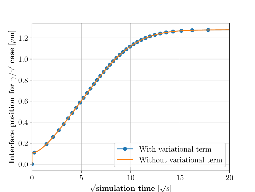
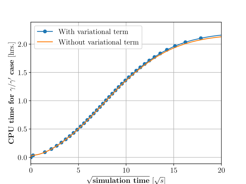
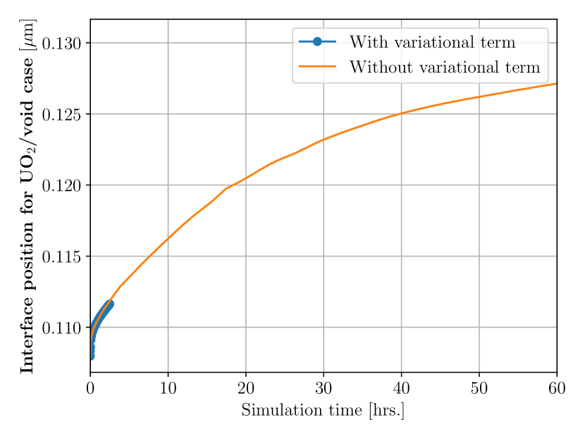
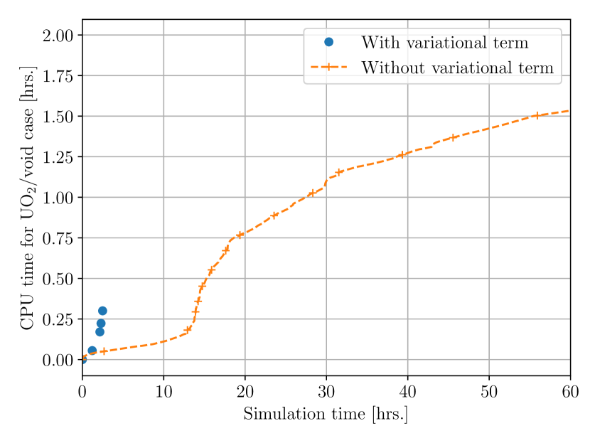
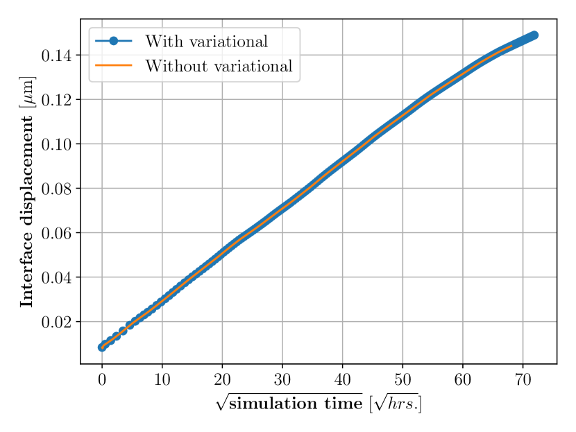
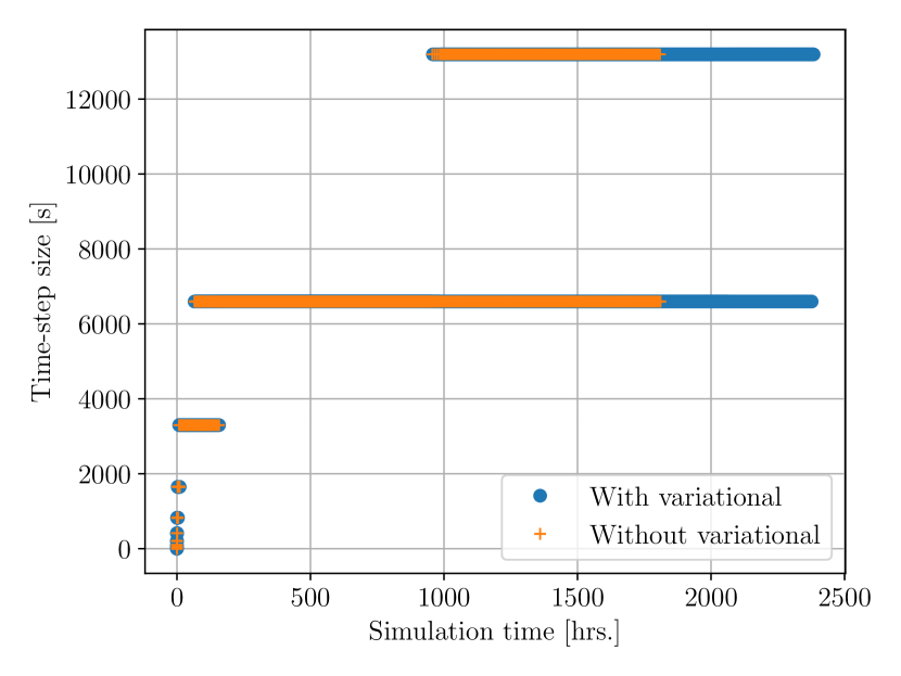
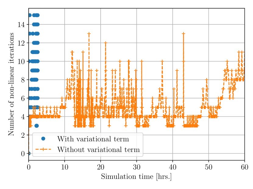

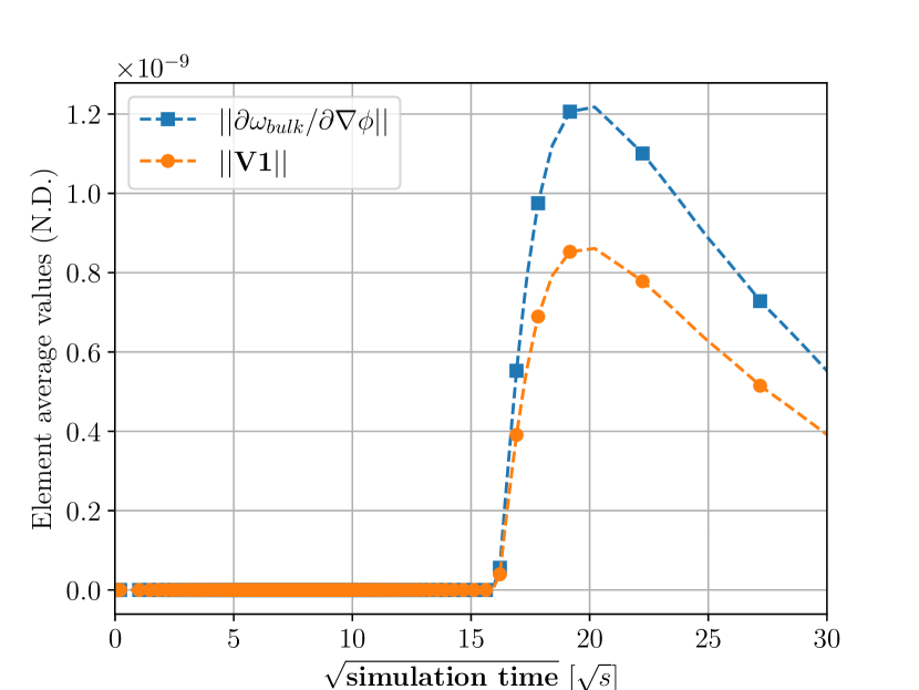
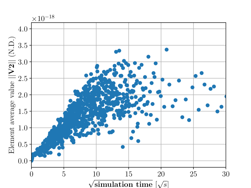
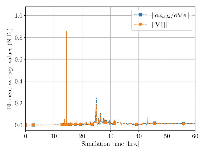
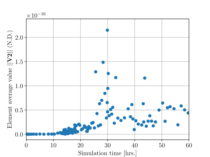
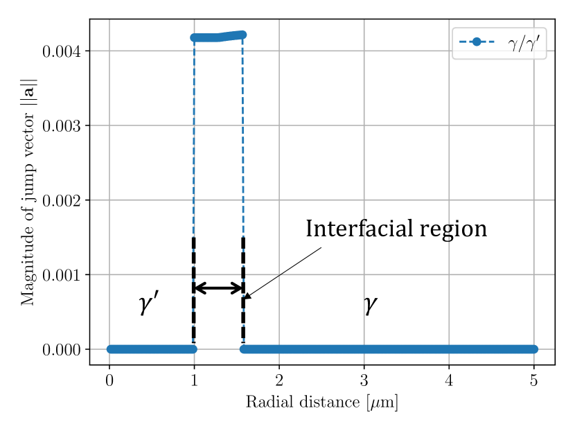
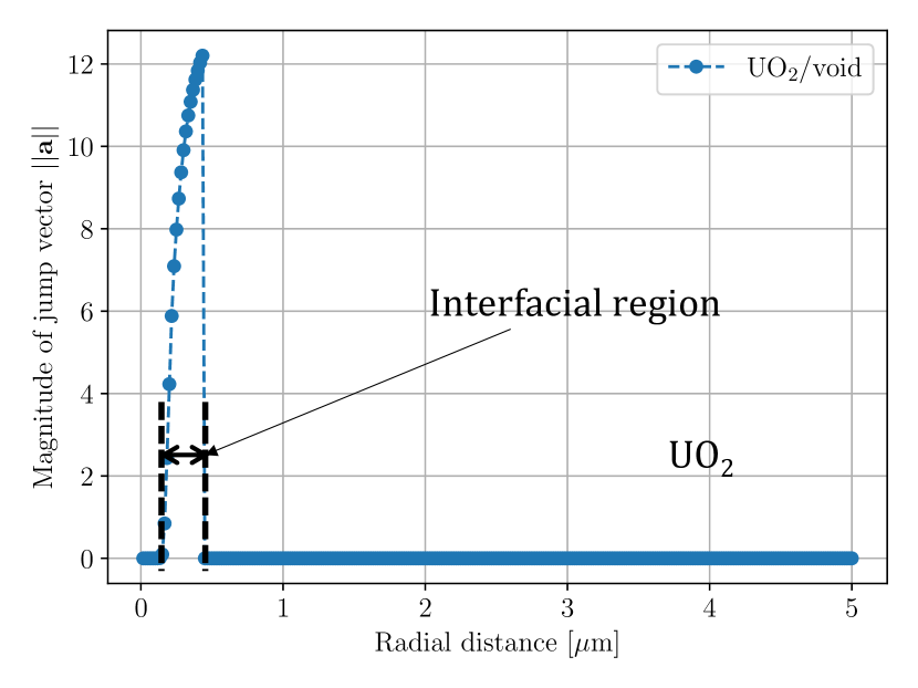
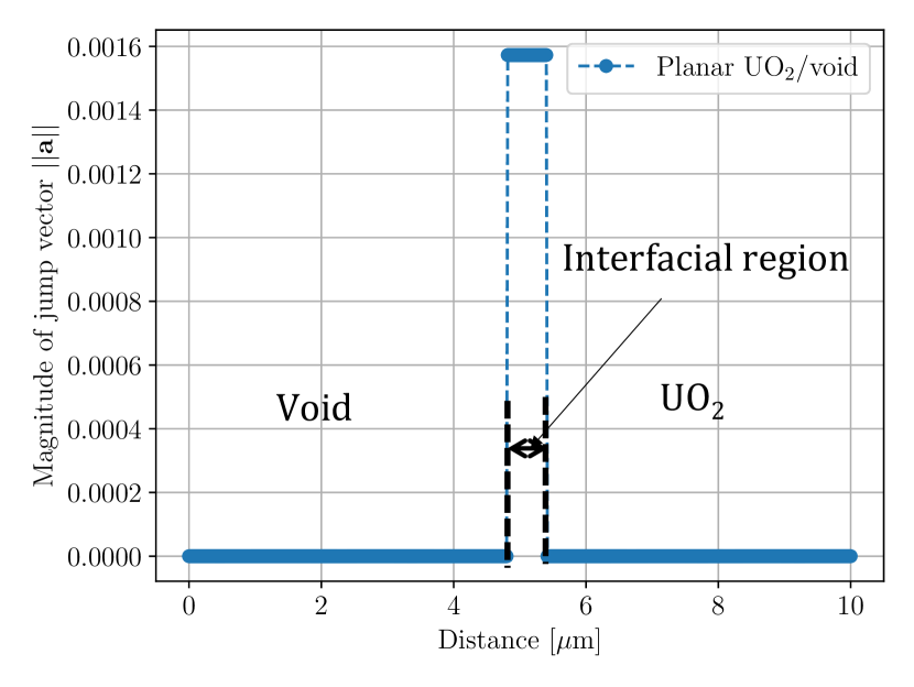
References
- Ardell and Nicholson [1966] A.J. Ardell and R.B. Nicholson. On the modulated structure of aged ni-al alloys: with an appendix on the elastic interaction between inclusions by j. d. eshelby. Acta Metallurgica, 14(10):1295–1309, 1966.
- Miyazaki and Doi [1989] Toru Miyazaki and Minoru Doi. Shape bifurcations in the coarsening of precipitates in elastically constrained systems. Materials Science and Engineering: A, 110:175–185, 1989.
- Marquis and Seidman [2001] E.A Marquis and D.N Seidman. Nanoscale structural evolution of al3sc precipitates in al(sc) alloys. Acta Materialia, 49(11):1909–1919, 2001.
- Lund and Voorhees [2002] A.C Lund and P.W Voorhees. The effects of elastic stress on microstructural development: the three-dimensional microstructure of a – alloy. Acta Materialia, 50(10):2585–2598, 2002.
- Sudbrack et al. [2008] Chantal K. Sudbrack, Tiffany D. Ziebell, Ronald D. Noebe, and David N. Seidman. Effects of a tungsten addition on the morphological evolution, spatial correlations and temporal evolution of a model ni–al–cr superalloy. Acta Materialia, 56(3):448–463, 2008.
- Johnson and Cahn [1984] W.C. Johnson and J.W. Cahn. Elastically induced shape bifurcations of inclusions. Acta Metallurgica, 32(11):1925–1933, 1984.
- Johnson et al. [1990] W.C. Johnson, T.A. Abinandanan, and P.W. Voorhees. The coarsening kinetics of two misfitting particles in an anisotropic crystal. Acta Metallurgica et Materialia, 38(7):1349–1367, 1990.
- Voorhees et al. [1992] P.W. Voorhees, G.B. McFadden, and W.C. Johnson. On the morphological development of second-phase particles in elastically-stressed solids. Acta Metallurgica et Materialia, 40(11):2979–2992, 1992.
- Socrate and Parks [1993] S. Socrate and D.M. Parks. Numerical determination of the elastic driving force for directional coarsening in ni-superalloys. Acta Metallurgica et Materialia, 41(7):2185–2209, 1993.
- Abinandanan and Johnson [1993a] T.A. Abinandanan and W.C. Johnson. Coarsening of elastically interacting coherent particles—i. theoretical formulation. Acta Metallurgica et Materialia, 41(1):17–25, 1993a.
- Su and Voorhees [1996] C.H. Su and P.W. Voorhees. The dynamics of precipitate evolution in elastically stressed solids—i. inverse coarsening. Acta Materialia, 44(5):1987–1999, 1996.
- Jou et al. [1997] H.-J. Jou, P.H. Leo, and J.S. Lowengrub. Microstructural evolution in inhomogeneous elastic media. Journal of Computational Physics, 131(1):109–148, 1997.
- Akaiwa et al. [2001] Norio Akaiwa, K. Thornton, and P.W. Voorhees. Large-scale simulations of microstructural evolution in elastically stressed solids. Journal of Computational Physics, 173(1):61–86, 2001.
- Thornton et al. [2004a] K. Thornton, Norio Akaiwa, and P.W. Voorhees. Large-scale simulations of ostwald ripening in elastically stressed solids: I. development of microstructure. Acta Materialia, 52(5):1353–1364, 2004a.
- Thornton et al. [2004b] K. Thornton, Norio Akaiwa, and P.W. Voorhees. Large-scale simulations of ostwald ripening in elastically stressed solids. ii. coarsening kinetics and particle size distribution. Acta Materialia, 52(5):1365–1378, 2004b.
- Li and Chen [1998] D.Y. Li and L.Q. Chen. Computer simulation of stress-oriented nucleation and growth of precipitates in al–cu alloys. Acta Materialia, 46(8):2573–2585, 1998.
- Vaithyanathan and Chen [2002] V. Vaithyanathan and L.Q. Chen. Coarsening of ordered intermetallic precipitates with coherency stress. Acta Materialia, 50(16):4061–4073, 2002.
- Zhu et al. [2004] J.Z. Zhu, T. Wang, A.J. Ardell, S.H. Zhou, Z.K. Liu, and L.Q. Chen. Three-dimensional phase-field simulations of coarsening kinetics of particles in binary ni–al alloys. Acta Materialia, 52(9):2837–2845, 2004.
- Gururajan and Abinandanan [2007] M.P Gururajan and T.A Abinandanan. Phase field study of precipitate rafting under a uniaxial stress. Acta materialia, 55(15):5015–5026, 2007.
- Ardell [1972] A.J Ardell. The effect of volume fraction on particle coarsening: theoretical considerations. Acta Metallurgica, 20(1):61–71, 1972.
- Morral and Purdy [1994] J.E. Morral and G.R. Purdy. Particle coarsening in binary and multicomponent alloys. Scripta Metallurgica et Materialia, 30(7):905 – 908, 1994.
- Doi [1996] Minoru Doi. Elasticity effects on the microstructure of alloys containing coherent precipitates. Progress in Materials Science, 40(2):79–180, 1996.
- Fratzl et al. [1999] Peter Fratzl, Oliver Penrose, and Joel L Lebowitz. Modeling of phase separation in alloys with coherent elastic misfit. Journal of statistical physics, 95(5):1429–1503, 1999.
- Ardell [2014] Alan Ardell. The effects of elastic interactions on precipitate microstructural evolution in elastically inhomogeneous nickel-base alloys. Philosophical Magazine, 94, 04 2014.
- Fried and Gurtin [1999] Eliot Fried and Morton E Gurtin. Coherent solid-state phase transitions with atomic diffusion: a thermomechanical treatment. Journal of statistical physics, 95(5):1361–1427, 1999.
- Gurtin and Voorhees [1993] Morton E. Gurtin and Peter W. Voorhees. The continuum mechanics of coherent two-phase elastic solids with mass transport. Proceedings of the Royal Society. A, Mathematical and physical sciences, 440(1909):323–343, 1993.
- Voorhees and Johnson [2004] P. W. Voorhees and William C. Johnson. The thermodynamics of elastically stressed crystals, pages 1–201. Number C in Solid State Physics - Advances in Research and Applications. Academic Press Inc, c edition, 2004.
- Gurtin et al. [2010] M.E. Gurtin, E. Fried, and L. Anand. The Mechanics and Thermodynamics of Continua. Cambridge University Press, 2010.
- Abinandanan and Johnson [1993b] T.A. Abinandanan and W.C. Johnson. Coarsening of elastically interacting coherent particles—ii. simulations of preferential coarsening and particle migrations. Acta Metallurgica et Materialia, 41(1):27–39, 1993b.
- Duddu et al. [2011] Ravindra Duddu, David L. Chopp, Peter Voorhees, and Brian Moran. Diffusional evolution of precipitates in elastic media using the extended finite element and the level set methods. Journal of Computational Physics, 230(4):1249–1264, 2011.
- Zhao et al. [2015] Xujun Zhao, Stéphane P.A. Bordas, and Jianmin Qu. Equilibrium morphology of misfit particles in elastically stressed solids under chemo-mechanical equilibrium conditions. Journal of the Mechanics and Physics of Solids, 81:1–21, 2015.
- Wang et al. [1993] S.-L. Wang, R.F. Sekerka, A.A. Wheeler, B.T. Murray, S.R. Coriell, R.J. Braun, and G.B. McFadden. Thermodynamically-consistent phase-field models for solidification. Physica D: Nonlinear Phenomena, 69(1):189–200, 1993.
- Chen [2002] Long-Qing Chen. Phase-field models for microstructure evolution. Annual Review of Materials Research, 32(1):113–140, 2002.
- Khachaturyan [1983] Armen Gurgenovich Khachaturyan. Theory of structural transformations in solids. Wiley-interscience publications. Wiley, New York (N.Y.), 1983.
- Chen and Shen [1998] L.Q. Chen and Jie Shen. Applications of semi-implicit fourier-spectral method to phase field equations. Computer Physics Communications, 108(2):147–158, 1998.
- Hu and Chen [2001] S.Y. Hu and L.Q. Chen. A phase-field model for evolving microstructures with strong elastic inhomogeneity. Acta Materialia, 49(11):1879–1890, 2001.
- Plapp [2011] Mathis Plapp. Unified derivation of phase-field models for alloy solidification from a grand-potential functional. Phys. Rev. E, 84(3):031601–1–15, 2011.
- Karma [2001] Alain Karma. Phase-field formulation for quantitative modeling of alloy solidification. Phys. Rev. Lett., 87:115701, Aug 2001.
- Steinbach [2009] Ingo Steinbach. Phase-field models in materials science. Modelling and Simulation in Materials Science and Engineering, 17(7):073001, jul 2009.
- Plapp [2007] Mathis Plapp. Three-dimensional phase-field simulations of directional solidification. Journal of Crystal Growth, 303(1):49–57, 2007. Proceedings of the Fifth Workshop on Modeling in Crystal Growth.
- Tiaden et al. [1998] J. Tiaden, B. Nestler, H.J. Diepers, and I. Steinbach. The multiphase-field model with an integrated concept for modelling solute diffusion. Physica D: Nonlinear Phenomena, 115(1):73 – 86, 1998.
- Kim et al. [1999] Seong Gyoon Kim, Won Tae Kim, and Toshio Suzuki. Phase-field model for binary alloys. Phys. Rev. E, 60(6):7186–7197, 1999.
- Provatas and Elder [2011] N. Provatas and K. Elder. Phase-Field Methods in Materials Science and Engineering. Wiley, 2011.
- Steinbach and Apel [2006] I. Steinbach and M. Apel. Multi phase field model for solid state transformation with elastic strain. Physica D: Nonlinear Phenomena, 217(2):153 – 160, 2006.
- Eiken et al. [2006] J. Eiken, B. Böttger, and I. Steinbach. Multiphase-field approach for multicomponent alloys with extrapolation scheme for numerical application. Phys. Rev. E, 73(6):066122, Jun 2006.
- Durga et al. [2013] A Durga, P Wollants, and N Moelans. Evaluation of interfacial excess contributions in different phase-field models for elastically inhomogeneous systems. Modelling and simulation in materials science and engineering, 21(5):55018, 2013.
- Durga et al. [2015] A. Durga, P. Wollants, and N. Moelans. A quantitative phase-field model for two-phase elastically inhomogeneous systems. Computational Materials Science, 99:81–95, 2015.
- Schneider et al. [2015] Daniel Schneider, Oleg Tschukin, Abhik Choudhury, Michael Selzer, Thomas Böhlke, and Britta Nestler. Phase-field elasticity model based on mechanical jump conditions. Computational Mechanics, 55(5):887–901, May 2015.
- Schneider et al. [2017] Daniel Schneider, Felix Schwab, Ephraim Schoof, Andreas Reiter, Christoph Herrmann, Michael Selzer, Thomas Böhlke, and Britta Nestler. On the stress calculation within phase-field approaches: a model for finite deformations. Computational Mechanics, 60(2):203–217, Aug 2017.
- Svendsen et al. [2018] Bob Svendsen, Pratheek Shanthraj, and Dierk Raabe. Finite-deformation phase-field chemomechanics for multiphase, multicomponent solids. Journal of the Mechanics and Physics of Solids, 112:619–636, 2018.
- Tschukin et al. [2019] O. Tschukin, D. Schneider, and B. Nestler. An elasto-chemical phase-field model for isotropic solids. European Journal of Mechanics - A/Solids, 73:181–191, 2019.
- Kubendran Amos et al. [2018] P.G. Kubendran Amos, Ephraim Schoof, Daniel Schneider, and Britta Nestler. Chemo-elastic phase-field simulation of the cooperative growth of mutually-accommodating widmanstätten plates. Journal of Alloys and Compounds, 767:1141–1154, 2018.
- Schoof et al. [2020] Ephraim Schoof, P.G. Kubendran Amos, Daniel Schneider, and Britta Nestler. Influence of stress-free transformation strain on the autocatalytic growth of bainite: A multiphase-field analysis. Materialia, 9:100620, 2020.
- Mushongera et al. [2015] L.T. Mushongera, M. Fleck, J. Kundin, Y. Wang, and H. Emmerich. Effect of re on directional -coarsening in commercial single crystal ni-base superalloys: A phase field study. Acta Materialia, 93:60–72, 2015.
- Tschukin [2017] Oleg Tschukin. Phase-Field Modelling of Welding and of Elasticity-Dependent Phase Transformations. PhD thesis, Karlsruher Institut für Technologie (KIT), 2017.
- Mosler et al. [2014] J. Mosler, O. Shchyglo, and H. Montazer Hojjat. A novel homogenization method for phase field approaches based on partial rank-one relaxation. Journal of the Mechanics and Physics of Solids, 68:251 – 266, 2014.
- Bartels et al. [2021] Alexander Bartels, Patrick Kurzeja, and Jörn Mosler. Cahn–hilliard phase field theory coupled to mechanics: Fundamentals, numerical implementation and application to topology optimization. Computer Methods in Applied Mechanics and Engineering, 383:113918, 2021.
- Wheeler et al. [1992] A. A. Wheeler, W. J. Boettinger, and G. B. McFadden. Phase-field model for isothermal phase transitions in binary alloys. Phys. Rev. A, 45(10):7424–7439, May 1992.
- Kim et al. [1998] Seong Gyoon Kim, Won Tae Kim, and Toshio Suzuki. Interfacial compositions of solid and liquid in a phase-field model with finite interface thickness for isothermal solidification in binary alloys. Phys. Rev. E, 58(3):3316–3323, Sep 1998.
- Ammar [2010] Kais Ammar. Modelling and simulation of phase transformation-mechanics coupling using a phase field method. PhD thesis, École Nationale Supérieure des Mines de Paris, 01 2010.
- Cahn and Larché [1984] J.W. Cahn and F. Larché. A simple model for coherent equilibrium. Acta Metallurgica, 32(11):1915–1923, 1984.
- Aagesen et al. [2017] Larry K. Aagesen, Daniel Schwen, Karim Ahmed, and Michael R. Tonks. Quantifying elastic energy effects on interfacial energy in the kim-kim-suzuki phase-field model with different interpolation schemes. Computational Materials Science, 140:10–21, 2017.
- Simon et al. [2020] Pierre-Clément A. Simon, Larry K. Aagesen, Arthur T. Motta, and Michael R. Tonks. The effects of introducing elasticity using different interpolation schemes to the grand potential phase field model. Computational Materials Science, 183:109790, 2020.
- Eshelby [1957] J. D. Eshelby. The determination of the elastic field of an ellipsoidal inclusion, and related problems. Proceedings of the Royal Society of London. Series A, Mathematical and physical sciences, 241(1226):376–396, 1957.
- Mura [1991] Toshio Mura. Micromechanics of defects in solids. Kluwer academic, Dordrecht, 1991.
- Kiefer et al. [2017] B. Kiefer, T. Furlan, and J. Mosler. A numerical convergence study regarding homogenization assumptions in phase field modeling. International Journal for Numerical Methods in Engineering, 112(9):1097–1128, 2017.
- Bartels and Mosler [2017] Alexander Bartels and Jörn Mosler. Efficient variational constitutive updates for allen–cahn-type phase field theory coupled to continuum mechanics. Computer Methods in Applied Mechanics and Engineering, 317:55 – 83, 2017.
- Choudhury and Nestler [2012] Abhik Choudhury and Britta Nestler. Grand-potential formulation for multicomponent phase transformations combined with thin-interface asymptotics of the double-obstacle potential. Phys. Rev. E, 85(2):021602–1–16, 2012.
- Chatterjee and Moelans [2021] Sourav Chatterjee and Nele Moelans. A grand-potential based phase-field approach for simulating growth of intermetallic phases in multicomponent alloy systems. Acta Materialia, 206:116630, 2021.
- Choudhury et al. [2015] Abhik Choudhury, Michael Kellner, and Britta Nestler. A method for coupling the phase-field model based on a grand-potential formalism to thermodynamic databases. Current Opinion in Solid State and Materials Science, 19(5):287 – 300, 2015.
- Larché and Cahn [1985] F.C. Larché and J.W. Cahn. The interactions of composition and stress in crystalline solids. Acta metallurgica, 33(3):331–357, 1985.
- Allen and Cahn [1979] Samuel M. Allen and John W. Cahn. A microscopic theory for antiphase boundary motion and its application to antiphase domain coarsening. Acta Metallurgica, 27(6):1085 – 1095, 1979.
- Andersson and Ågren [1992] Jan‐Olof Andersson and John Ågren. Models for numerical treatment of multicomponent diffusion in simple phases. Journal of Applied Physics, 72(4):1350–1355, 1992.
- Gaston et al. [2009] Derek Gaston, Chris Newman, Glen Hansen, and Damien Lebrun-Grandié. Moose: A parallel computational framework for coupled systems of nonlinear equations. Nuclear Engineering and Design, 239(10):1768 – 1778, 2009.
- Schwen et al. [2017] D. Schwen, L.K. Aagesen, J.W. Peterson, and M.R. Tonks. Rapid multiphase-field model development using a modular free energy based approach with automatic differentiation in moose/marmot. Computational Materials Science, 132:36 – 45, 2017.
- Larché and Cahn [1978] Francis Larché and John W. Cahn. A nonlinear theory of thermochemical equilibrium of solids under stress. Acta Metallurgica, 26(1):53–60, 1978.
- Kim [2007] Seong Gyoon Kim. A phase-field model with antitrapping current for multicomponent alloys with arbitrary thermodynamic properties. Acta Materialia, 55(13):4391–4399, 2007.
- Greenquist et al. [2020] Ian Greenquist, Michael R. Tonks, Larry K. Aagesen, and Yongfeng Zhang. Development of a microstructural grand potential-based sintering model. Computational Materials Science, 172:109288, 2020.
- Sonderegger and Kozeschnik [2009] B. Sonderegger and E. Kozeschnik. Generalized nearest-neighbor broken-bond analysis of randomly oriented coherent interfaces in multicomponent fcc and bcc structures. Metallurgical and Materials Transactions A, 40(3):499–510, Mar 2009.
- NIST [2002] NIST. Elastic moduli data for polycrystalline ceramics, https://srdata.nist.gov/ceramicdataportal/elasticity/uo2, 2002.
- Johnson [1987] William C. Johnson. Precipitate shape evolution under applied stress—thermodynamics and kinetics. Metallurgical and Materials Transactions A, 18(2):233–247, Feb 1987.
- Wu [2001] Chien H. Wu. The role of eshelby stress in composition-generated and stress-assisted diffusion. Journal of the Mechanics and Physics of Solids, 49(8):1771–1794, 2001.
- Fährmann et al. [1995] M. Fährmann, P. Fratzl, O. Paris, E. Fährmann, and William C. Johnson. Influence of coherency stress on microstructural evolution in model ni-al-mo alloys. Acta Metallurgica et Materialia, 43(3):1007–1022, 1995.
- Abeyaratne and Knowles [1990] Rohan Abeyaratne and James K. Knowles. On the driving traction acting on a surface of strain discontinuity in a continuum. Journal of the Mechanics and Physics of Solids, 38(3):345–360, 1990.
- Johnson and Alexander [1986] William C. Johnson and J. Iwan D. Alexander. Interfacial conditions for thermomechanical equilibrium in two‐phase crystals. Journal of Applied Physics, 59(8):2735–2746, 1986.