Graph state-space models

Abstract

State-space models constitute an effective modeling tool to describe multivariate time series and operate by maintaining an updated representation of the system state from which predictions are made. Within this framework, relational inductive biases, e.g., associated with functional dependencies existing among signals, are not explicitly exploited leaving unattended great opportunities for effective modeling approaches. The manuscript aims, for the first time, at filling this gap by matching state-space modeling and spatio-temporal data where the relational information, say the functional graph capturing latent dependencies, is learned directly from data and is allowed to change over time. Within a probabilistic formulation that accounts for the uncertainty in the data-generating process, an encoder-decoder architecture is proposed to learn the state-space model end-to-end on a downstream task. The proposed methodological framework generalizes several state-of-the-art methods and demonstrates to be effective in extracting meaningful relational information while achieving optimal forecasting performance in controlled environments.

1 Introduction

Decades of research and real-world problem solutions have shown that state-space representations provide compact and amenable formulations for describing time-invariant time series, e.g., whenever the data-generating process can be structured as a system of differential equations (Durbin and Koopman, 2012). This stochastic process, considered here to be nonlinear to address the general case, can be modeled as

$$\begin{cases}\boldsymbol{\mathbf{h}}_{t}=f_{\textsc{st}}(\boldsymbol{\mathbf{h}}_{t-1},\boldsymbol{\mathbf{x}}_{t},\eta_{t})&\qquad\boldsymbol{\mathbf{x}}_{t}\in\mathbb{R}^{d_{x}},\boldsymbol{\mathbf{h}}_{t}\in\mathbb{R}^{d_{h}}\\ \boldsymbol{\mathbf{y}}_{t}=f_{\textsc{ro}}(\boldsymbol{\mathbf{h}}_{t},\nu_{t})&\qquad\boldsymbol{\mathbf{y}}_{t}\in\mathbb{R}^{d_{y}}\end{cases}$$ (1)

where, at each time step $t$, $\boldsymbol{\mathbf{x}}_{t}$ is the input, $\boldsymbol{\mathbf{h}}_{t}$ the system state, and $\boldsymbol{\mathbf{y}}_{t}$ the system output. Stochastic process (1) starts with initial state $\boldsymbol{\mathbf{h}}_{0}\sim P_{\boldsymbol{\mathbf{h}}_{0}}$; white noise stochastic processes $\{\eta_{t}\}_{t}$ and $\{\nu_{t}\}_{t}$ model the uncertainty at state and output level, respectively.

Indeed, predictive families of state-space models of the form

$$\begin{cases}\boldsymbol{\mathbf{h}}_{t}\sim P^{t}_{\theta}\doteq\mathbb{P}(\boldsymbol{\mathbf{h}}\mid\boldsymbol{\mathbf{h}}_{t-1},\boldsymbol{\mathbf{x}}_{t};{\theta})&\qquad\boldsymbol{\mathbf{x}}_{t}\in\mathbb{R}^{d_{x}},\boldsymbol{\mathbf{h}}_{t}\in\mathbb{R}^{d_{h}}\\ \hat{\boldsymbol{\mathbf{y}}}_{t}\sim P^{t}_{\psi}\doteq\mathbb{P}(\hat{\boldsymbol{\mathbf{y}}}\mid\boldsymbol{\mathbf{h}}_{t};\psi)&\qquad\hat{\boldsymbol{\mathbf{y}}}_{t}\in\mathbb{R}^{d_{y}}\end{cases}$$ (2)

have been demonstrated effective in learning the process in (1) and are used, mostly in a linear setup, in vast domains ranging from control theory to machine learning (e.g., see Hochreiter and Schmidhuber (1997); Chen et al. (2017); Brunton et al. (2016, 2021)); Kalman filters (Kalman, 1960; Kalman and Bucy, 1961) are a particularly relevant case and have attracted significant attention among researchers and practitioners. Predictors in (2) are probabilistic, with $P^{t}_{\theta}$ and $P^{t}_{\psi}$ probability distributions parametrized by vectors $\theta$ and $\psi$, respectively. Whenever the interest is in point estimates, e.g., the forecast of future system outputs, the prediction is derived from a statistic of the probability distribution

$$P_{\psi,\theta}^{t}\doteq\mathbb{P}(\hat{\boldsymbol{\mathbf{y}}}\mid\boldsymbol{\mathbf{x}}_{t},\dots,\boldsymbol{\mathbf{x}}_{1},\boldsymbol{\mathbf{h}}_{0};\theta,\psi),$$ (3)

or, by introducing the state variable,

$$\mathbb{P}(\hat{\boldsymbol{\mathbf{y}}}\mid\boldsymbol{\mathbf{x}}_{t},\boldsymbol{\mathbf{h}}_{t-1};\theta,\psi).$$ (4)

Common examples of statistics are the expectation

$$\hat{\boldsymbol{\mathbf{y}}}_{t}=\mathbb{E}_{\hat{\boldsymbol{\mathbf{y}}}\sim P_{\theta,\psi}^{t}}[\hat{\boldsymbol{\mathbf{y}}}]$$ (5)

yielding the optimal $2$-norm value; the mode of $P_{\theta,\psi}^{t}$, i.e., providing the maximum likelihood estimate $\hat{\boldsymbol{\mathbf{y}}}_{t}$; and the quantile at a given level $\alpha$

$$\hat{\boldsymbol{\mathbf{y}}}_{t}:\mathbb{P}_{\hat{\boldsymbol{\mathbf{y}}}\sim P_{\theta,\psi}^{t}}(\hat{\boldsymbol{\mathbf{y}}}\leq\hat{\boldsymbol{\mathbf{y}}}_{t})=\alpha,$$ (6)

for scalar outputs. We comment that the general formulation in (2) allows for handling generative tasks too.

Research has evidenced that incorporating existing relational information in learned time-series models often offers an important inductive bias that has led to major performance improvements, e.g., in multistep-ahead forecasting (Seo et al., 2018; Li et al., 2018) and missing values imputation (Cini et al., 2021; Marisca et al., 2022; Chen et al., 2022); these achievements follow important advances in signal processing and deep learning for graph-structured data — see (Bronstein et al., 2017; Stankovic et al., 2019; Bacciu et al., 2020; Bronstein et al., 2021) for a comprehensive overview of the subject.

In several application scenarios, relations in space and/or time are available as prior information, e.g., as domain knowledge; in others, relational dependencies are unavailable and, within this challenging setup, the latent graph structure has to be learned directly from measurements (Kipf et al., 2018; Wu et al., 2019; Kazi et al., 2022; Cini et al., 2022).

This paper introduces a novel generalized state-space formulation for spatio-temporal time series prediction where inputs, states, and outputs can be structured as graphs. The graph topology and nodes are allowed to vary over time and be decoupled between inputs, states and outputs, thus yielding a flexible framework able to learn unknown relationships among both observed and latent entities while, at the same time, discarding spurious dependencies through proper regularization. A schematic description of the considered framework is given in Figure 1.

The principal novel contributions can be summarized as follows:

• We provide a general probabilistic state-space framework for spatio-temporal time series modeling where input, output, and state representations are attributed graphs, whose topology and number of nodes are allowed to change over time [Section 2].

• An end-to-end learning procedure is given that accounts for the stochastic nature of state and output graphs. Latent graph states are directly learned from the time series by means of gradient-based optimization of the parametric graph distributions [Section 3].

• We derive popular state-of-the-art methods tailored to different application settings as instances of the proposed framework [Section 4].

Empirical evidence shows that the proposed state-space framework and learning procedure allows the practitioner to achieve optimal performance on different tasks as well as extract information referable to latent state dynamics [Section 5].

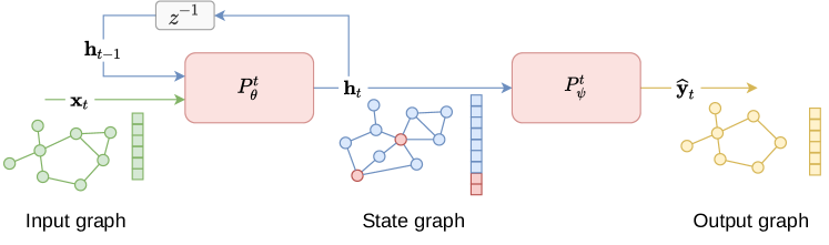
Figure 1: High-level representation of the graph-based predictive family of state-space models, following the structure of (7). State graph $\boldsymbol{\mathbf{h}}_{t}$ is the processing outcome of input graph $\boldsymbol{\mathbf{x}}_{t}$ and previous state $\boldsymbol{\mathbf{h}}_{t-1}=z^{-1}\boldsymbol{\mathbf{h}}_{t}$; $z^{-1}$ being the lag (backshift) operator. Output graph $\boldsymbol{\mathbf{y}}_{t}$ follows from state graph $\boldsymbol{\mathbf{h}}_{t}$. Each graph is associated with a stack of node-level signals (scalar values in the figure) represented by the array drawn beside the graph. Note that input, state, and output graphs can differ over time both in terms of edges and number of nodes.

2 Graph state-space models

In this section, we derive the proposed state-space formulation that generalizes vector representations of (2) to the case where inputs $\boldsymbol{\mathbf{x}}_{t}$, outputs $\boldsymbol{\mathbf{y}}_{t}$, and states $\boldsymbol{\mathbf{h}}_{t}$ are graphs. As we will show, the derivation is not trivial; indeed, the vector setup follows as a special case when no topological/relational information is given and the latent state is collapsed to a single entity. (2) can be advantageously extended to the graph case by considering the discrete-time stochastic data-generating process $\mathcal{P}$

$$\begin{cases}\boldsymbol{\mathbf{h}}_{t}=f_{\textsc{st}}(\boldsymbol{\mathbf{h}}_{t-1},\boldsymbol{\mathbf{x}}_{t},\eta_{t})&\qquad\boldsymbol{\mathbf{x}}_{t}\in\mathcal{X},\boldsymbol{\mathbf{h}}_{t}\in\mathcal{H}\\ \boldsymbol{\mathbf{y}}_{t}=f_{\textsc{ro}}(\boldsymbol{\mathbf{h}}_{t},\nu_{t})&\qquad\boldsymbol{\mathbf{y}}_{t}\in\mathcal{Y};\end{cases}$$ (7)

inputs, states, and outputs belong to graph spaces $\mathcal{X},\mathcal{H}$, and $\mathcal{Y}$, respectively. The input graph $\boldsymbol{\mathbf{x}}_{t}$ at time $t$ is defined over a set $V(\boldsymbol{\mathbf{x}}_{t})$ of sensors associated with the graph nodes and the edge set $E(\boldsymbol{\mathbf{x}}_{t})\subseteq V(\boldsymbol{\mathbf{x}}_{t})\times V(\boldsymbol{\mathbf{x}}_{t})$ encoding relations existing among nodes, such as physical proximity, signal correlations, or causal dependencies; we refer to them as spatial relations to define a generic domain decoupled from the temporal axis. We denote the associated graph signal as $s(\boldsymbol{\mathbf{x}}_{t})=\{s_{v}(\boldsymbol{\mathbf{x}}_{t})\in\mathbb{R}^{d_{x}}:v\in V(\boldsymbol{\mathbf{x}}_{t})\}$, with $s_{v}(\boldsymbol{\mathbf{x}}_{t})$ being the signal at node $v$. Node signals, topology, and node set can change with time; denote with $\mathbb{V}_{\boldsymbol{\mathbf{x}}}=\bigcup_{t}V(\boldsymbol{\mathbf{x}}_{t})$ the union set of all nodes whose cardinality is assumed to be finite. A visual representation of the resulting graph-based spatio-temporal data sequence $\boldsymbol{\mathbf{x}}_{1},\boldsymbol{\mathbf{x}}_{2},\dots,\boldsymbol{\mathbf{x}}_{t},\dots$ is provided in Figure 2.

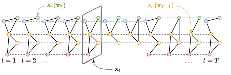
Figure 2: An example of a spatio-temporal data over a set $\mathbb{V}_{\boldsymbol{\mathbf{x}}}$ of 5 nodes. Graph $\boldsymbol{\mathbf{x}}_{t}$ is given at each step $t$. $\boldsymbol{\mathbf{x}}_{t}$ is defined over a node set $V(\boldsymbol{\mathbf{x}}_{t})\subseteq\mathbb{V}_{\boldsymbol{\mathbf{x}}}$ and has node signals $s_{v}(\boldsymbol{\mathbf{x}}_{t})\in\mathbb{R}^{d_{x}}$ associated with each given node.

Given sequence $\{\boldsymbol{\mathbf{x}}_{t}\}_{t}$ with node set $\mathbb{V}_{\boldsymbol{\mathbf{x}}}$, we aim at predicting output graph $\boldsymbol{\mathbf{y}}_{t}$ at each time step $t$. Node set $\mathbb{V}_{\boldsymbol{\mathbf{y}}}=\bigcup_{t}V(\boldsymbol{\mathbf{y}}_{t})$ is not necessarily equal to $\mathbb{V}_{\boldsymbol{\mathbf{x}}}$ hence allowing for modeling several settings. For instance, in standard multivariate time series, we generally have a regular sampling for all nodes ($V(\boldsymbol{\mathbf{x}}_{t})=\mathbb{V}_{\boldsymbol{\mathbf{x}}}\ \forall t$) and, typically, associated relational information is unavailable ($E(\boldsymbol{\mathbf{x}}_{t})=\emptyset\ \forall t$). Other examples refer to systems where the sensors (nodes) are interconnected ($E(\boldsymbol{\mathbf{x}}_{t})\neq\emptyset\ \forall t$) (Alippi, 2014) or to social networks where new users subscribe while existing ones make new connections and change interests ($V(\boldsymbol{\mathbf{x}}_{t})$ and $E(\boldsymbol{\mathbf{x}}_{t})$ vary with time), e.g., see (Trivedi et al., 2019; Kazemi et al., 2020). Depending on the specific application, $\boldsymbol{\mathbf{y}}_{t}$ might be a scalar or a vector encoding of graph-level quantities. In a node-level forecasting scenario, instead, we might set $\boldsymbol{\mathbf{y}}_{t}\doteq s(\boldsymbol{\mathbf{x}}_{t+H})$ or $\boldsymbol{\mathbf{y}}_{t}\doteq[s(\boldsymbol{\mathbf{x}}_{t+1}),\dots,s(\boldsymbol{\mathbf{x}}_{t+H})]$, with integer $H>1$, accounting for multistep-ahead prediction tasks. Finally, exogenous variables, like those referring to extra sensor information or functional relations, can be included as well and encoded in $\boldsymbol{\mathbf{x}}_{t}$ to avoid overwhelming notation in the remainder of the paper.

In line with (2), we introduce the stochastic state-space family of predictive models

$$\begin{cases}\boldsymbol{\mathbf{h}}_{t}\sim P^{t}_{\theta}\doteq\mathbb{P}(\boldsymbol{\mathbf{h}}\mid\boldsymbol{\mathbf{h}}_{t-1},\boldsymbol{\mathbf{x}}_{t};{\theta}),&\qquad\boldsymbol{\mathbf{x}}_{t}\in\mathcal{X},\boldsymbol{\mathbf{h}}_{t}\in\mathcal{H}\\ \hat{\boldsymbol{\mathbf{y}}}_{t}\sim P^{t}_{\psi}\doteq\mathbb{P}(\hat{\boldsymbol{\mathbf{y}}}\mid\boldsymbol{\mathbf{h}}_{t};\psi),&\qquad\hat{\boldsymbol{\mathbf{y}}}_{t}\in\mathcal{Y}\end{cases}$$ (8)

which is fitted on realizations of process $\mathcal{P}$ to provide the output graph $\hat{\boldsymbol{\mathbf{y}}}_{t}$ given the input one; a schematic view is given in Figure 1. Denote with $\mathbb{V}_{\boldsymbol{\mathbf{h}}}$ the set of all state nodes; initial condition $\boldsymbol{\mathbf{h}}_{0}$ is drawn from a given prior distribution $P_{\boldsymbol{\mathbf{h}}_{0}}$. Differently from (7) where the randomness associated with the state vector $\boldsymbol{\mathbf{h}}_{t}$ is introduced by noise $\eta_{t}$, in (8) we formulate the state transition directly as $P_{\theta}^{t}$, i.e., as a graph probability distribution parametrized by vector $\theta$ and conditioned on previous state graph $\boldsymbol{\mathbf{h}}_{t-1}$ and input graph $\boldsymbol{\mathbf{x}}_{t}$. Similarly, the readout function is formulated as a graph probability distribution $P_{\psi}^{t}$ parametrized by $\psi$ and conditioned on the current state $\boldsymbol{\mathbf{h}}_{t}$.

After commenting on the relationships among graphs in input, output, and as states [Section 2.1], the following subsections present the proposed encoder-decoder architecture implementing (8) with the encoder module accounting for the state transition distribution [Section 2.2] and the decoder modeling the state-to-output distribution [Section 2.3].

2.1 Relationships among input, state, and output nodes

Node sets $V(\boldsymbol{\mathbf{x}}_{t})$ and $V(\boldsymbol{\mathbf{x}}_{t^{\prime}})$ might be different but, typically, $V(\boldsymbol{\mathbf{x}}_{t})\cap V(\boldsymbol{\mathbf{x}}_{t^{\prime}})\neq\emptyset$ implying some partial correspondence among groups of nodes; see Figure 2 for a visual example. When this is the case, $s(\boldsymbol{\mathbf{x}}_{t:T})$ denotes the tensor $[s(\boldsymbol{\mathbf{x}}_{t}),\dots,s(\boldsymbol{\mathbf{x}}_{T-1})]\in\mathbb{R}^{|\mathbb{V}_{\boldsymbol{\mathbf{x}}}|\times d_{x}\times(T-t)}$ obtained by stacking together all graph signals and appropriately masking out missing nodes at each time step; analogously, sequences of outputs and states are denoted by $s(\boldsymbol{\mathbf{y}}_{t:T})$ and $s(\boldsymbol{\mathbf{h}}_{t:T})$, respectively.

Note that we are not assuming identified nodes among sets $\mathbb{V}_{\boldsymbol{\mathbf{x}}},\mathbb{V}_{\boldsymbol{\mathbf{h}}}$, and $\mathbb{V}_{\boldsymbol{\mathbf{y}}}$, although this might be the case in some scenarios. For instance, if $\boldsymbol{\mathbf{y}}_{t}$ is interpreted to be a partial observation of $\boldsymbol{\mathbf{h}}_{t}$ as in Figure 3(c), then $\mathbb{V}_{\boldsymbol{\mathbf{y}}}\subseteq\mathbb{V}_{\boldsymbol{\mathbf{h}}}$. Differently, in the factor analysis setting the two sets $\mathbb{V}_{\boldsymbol{\mathbf{h}}}$ and $\mathbb{V}_{\boldsymbol{\mathbf{y}}}$ might be disjoint, see Figure 3(b). The proposed formulation is general and encompasses several successful models for time series analysis, some of which are described in Section 4; other examples are given in Figure 3.

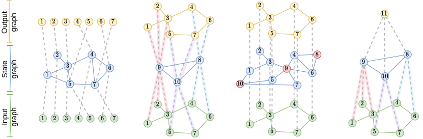
(a)

(b)

(c)

(d)

Figure 3: Some examples of possible configurations of the input, state, and output graphs and node correspondence for different problem settings. Dashed lines and node numbering encode the correspondence between nodes in sets $\mathbb{V}_{\boldsymbol{\mathbf{x}}},\mathbb{V}_{\boldsymbol{\mathbf{h}}}$, and $\mathbb{V}_{\boldsymbol{\mathbf{y}}}$. 3(a)) Node-level prediction with relational inference: $\mathbb{V}_{\boldsymbol{\mathbf{x}}}=\mathbb{V}_{\boldsymbol{\mathbf{h}}}=\mathbb{V}_{\boldsymbol{\mathbf{y}}}$; $\boldsymbol{\mathbf{x}}_{t}$ comes with no relational information which is learned directly from data and associated to $\boldsymbol{\mathbf{h}}_{t}$. 3(b)) Learning hidden factors (latent features) for unsupervised learning: $\boldsymbol{\mathbf{x}}_{t}=\boldsymbol{\mathbf{y}}_{t}$, with one-to-many relations existing from $\mathbb{V}_{\boldsymbol{\mathbf{h}}}$ to $\mathbb{V}_{\boldsymbol{\mathbf{x}}}$ such that node signals in $\boldsymbol{\mathbf{h}}_{t}$ are interpreted as hidden factors driving the dynamics of observation $\boldsymbol{\mathbf{x}}_{t}$. 3(c)) Time series forecasting with partial state observation and unknown relations: node correspondence across the three graphs, partial with hidden nodes ($\mathbb{V}_{\boldsymbol{\mathbf{x}}}=\mathbb{V}_{\boldsymbol{\mathbf{y}}}\subset\mathbb{V}_{\boldsymbol{\mathbf{h}}}$); $\boldsymbol{\mathbf{y}}_{t}=\boldsymbol{\mathbf{x}}_{t+1}$, $\boldsymbol{\mathbf{x}}_{t}$ has a graph structure, but additional relations are learned with $\boldsymbol{\mathbf{h}}_{t}$. 3(d)) Graph-level prediction: information from all sensors in $\mathbb{V}_{\boldsymbol{\mathbf{x}}}$ is transformed into a smaller set $\mathbb{V}_{\boldsymbol{\mathbf{h}}}$; a single output is returned.

2.2 Encoder module

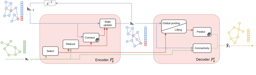
Figure 4: Block diagram of the encoder and decoder components described in Sections 2.2 and 2.3, respectively.

The encoder module processes graphs defined over potentially different node sets $\mathbb{V}_{\boldsymbol{\mathbf{x}}}$ and $\mathbb{V}_{\boldsymbol{\mathbf{h}}}$, and provides graph $\boldsymbol{\mathbf{h}}_{t}$ over set $\mathbb{V}_{\boldsymbol{\mathbf{h}}}$. A multitude of learnable graph-to-graph mapping methods has been proposed in the last years following different application needs. Notably, Grattarola et al. (2022) review and suggest graph pooling operators to achieve these mappings through a flexible formalism, called SRC. In the sequel, we adopt the general SRC framework combined with the message-passing paradigm to implement the encoder module, as shown in Figure 4; we stress that each select, reduce, and connect operator of the SRC framework is learnable and its parameters contribute to vector $\theta$ and that SRC offers a blueprint for the required processing steps without prescribing a particular implementation.

The first processing step consists in applying the select operator which defines a correspondence among nodes in $\mathbb{V}_{\boldsymbol{\mathbf{x}}}$ and those in $\mathbb{V}_{\boldsymbol{\mathbf{h}}}$. Typically, this is modeled by an affiliation matrix

$$\boldsymbol{\mathbf{S}}_{t}=\textsc{Select}(\boldsymbol{\mathbf{x}}_{t};\theta)\in\mathbb{R}^{|\mathbb{V}_{\boldsymbol{\mathbf{h}}}|\times|\mathbb{V}_{\boldsymbol{\mathbf{x}}}|}.$$ (9)

A possible choice for the select function consists in exploiting an MLP to compute the affiliation matrix, i.e., $\boldsymbol{\mathbf{S}}_{t}=\textsc{MLP}(\boldsymbol{\mathbf{x}}_{t};\theta)$ (see the MinCutPool approach (Bianchi et al., 2020)). Other choices include operators explicitly relying on the topology of the input graph $\boldsymbol{\mathbf{x}}_{t}$ (Ying et al., 2018) and hard-coded affiliation matrices where appropriate node correspondences are set at design time; for instance, in the setup of Figure 3(a), $\boldsymbol{\mathbf{S}}_{t}$ could be the identity matrix.

The second step consists of applying the reduce operation

$$(\boldsymbol{\mathbf{z}}_{t}^{\prime},V_{t})=\textsc{Reduce}(\boldsymbol{\mathbf{x}}_{t},\boldsymbol{\mathbf{S}}_{t};\theta)$$ (10)

which constructs intermediate node representations $\boldsymbol{\mathbf{z}}_{t}^{\prime}$ for the nodes in $V_{t}\subseteq\mathbb{V}_{\boldsymbol{\mathbf{h}}}$ from node signals in $\boldsymbol{\mathbf{x}}_{t}$ as determined by the affiliation matrix $\boldsymbol{\mathbf{S}}_{t}$; a common choice is $\boldsymbol{\mathbf{z}}_{t}^{\prime}=\boldsymbol{\mathbf{S}}_{t}s(\boldsymbol{\mathbf{x}}_{t})$. Then, $\boldsymbol{\mathbf{z}}_{t}^{\prime}$ is concatenated with the previous node states $s(\boldsymbol{\mathbf{h}}_{t-1})$ along the features dimension, i.e., $\boldsymbol{\mathbf{z}}_{t}^{\prime\prime}=\left[\left.\boldsymbol{\mathbf{z}}_{t}^{\prime}\,\right\rVert\,s(\boldsymbol{\mathbf{h}}_{t-1})\right].$ At last, the connect operation outputs the connectivity between pairs of nodes in $\boldsymbol{\mathbf{h}}_{t}$. We consider a probabilistic model for the edges $E_{t}=E(\boldsymbol{\mathbf{h}}_{t})$ of $\boldsymbol{\mathbf{h}}_{t}$ where

$$E_{t}\sim P_{\textsc{Con}}\doteq\mathbb{P}\left(E\mid\boldsymbol{\mathbf{z}}_{t}^{\prime\prime},E(\boldsymbol{\mathbf{h}}_{t-1});\theta\right)$$ (11)

follows a learnable parametric distribution $P_{\textsc{Con}}$ conditioned on $\boldsymbol{\mathbf{z}}_{t}^{\prime\prime}$ and $E(\boldsymbol{\mathbf{h}}_{t-1})$. In this paper, we consider the Binary Edge Sampler (BES) proposed by Cini et al. (2022) where all edges are sampled from independent Bernoulli random variables whose parameters are stored in matrix $\Phi=\Phi(\boldsymbol{\mathbf{z}}_{t}^{\prime\prime},E(\boldsymbol{\mathbf{h}}_{t-1}))\in[0,1]^{|V_{t}|\times|V_{t}|}$.

Finally, state graph $\boldsymbol{\mathbf{h}}_{t}\sim P_{\theta}^{t}$ at time step $t$ is then $\boldsymbol{\mathbf{h}}_{t}\doteq(V_{t},E_{t},\boldsymbol{\mathbf{z}}_{t}^{\prime\prime\prime})$, where $\boldsymbol{\mathbf{z}}_{t}^{\prime\prime\prime}$ is obtained as output of a (multi-layer) message-passing neural network (MPNN) (Gilmer et al., 2017)

$$\boldsymbol{\mathbf{z}}_{t}^{\prime\prime\prime}=\textsc{MPNN}\left(E_{t},\boldsymbol{\mathbf{z}}_{t}^{\prime\prime};\theta\right).$$ (12)

2.3 Decoder module

The decoder (prediction) module, can be implemented in different ways, according to whether $\boldsymbol{\mathbf{y}}_{t}$ is a graph-level or a node-level output. In the case of graph-level outputs, we consider a global pooling operator (Grattarola et al., 2022) applied to state graph $\boldsymbol{\mathbf{h}}_{t}$ to generate vector $\boldsymbol{\mathbf{r}}_{t}=\textsc{GlobalPooling}(\boldsymbol{\mathbf{h}}_{t})$. Then, the predictive distribution $P_{\psi}^{t}$ in (8) is given as the parametric distribution

$$P_{\psi}^{t}=\mathbb{P}(\hat{\boldsymbol{\mathbf{y}}}\mid\boldsymbol{\mathbf{r}}_{t};\psi)$$ (13)

conditioned on the state-to-output vector $\boldsymbol{\mathbf{r}}_{t}$. Differently, for node-level outputs, we need to map node set $\mathbb{V}_{\boldsymbol{\mathbf{h}}}$ to $\mathbb{V}_{\boldsymbol{\mathbf{x}}}$. This lifting operation, known also as upscaling when $|\mathbb{V}_{\boldsymbol{\mathbf{h}}}|<|\mathbb{V}_{\boldsymbol{\mathbf{x}}}|$ (Grattarola et al., 2022), can be carried out as $\boldsymbol{\mathbf{r}}_{t}=\boldsymbol{\mathbf{S}}_{t}^{+}s(\boldsymbol{\mathbf{h}}_{t})$, where $\boldsymbol{\mathbf{S}}_{t}^{+}$ is the pseudo-inverse of selection matrix $\boldsymbol{\mathbf{S}}_{t}$ considered in the select operation of the encoder.

The predictive distribution $P_{\psi}^{t}$ of (8) conditioned on $\boldsymbol{\mathbf{r}}_{t}$ and $E_{t}$ is then derived as

$$\hat{\boldsymbol{\mathbf{y}}}_{t}=g_{\psi}(\boldsymbol{\mathbf{r}}_{t},E_{t},\epsilon_{t}),\qquad\epsilon_{t}\sim P_{\epsilon},$$ (14)

where $g_{\psi}$ is a differentiable function and $P_{\epsilon}$ a predefined distribution, e.g., a multivariate standard Gaussian distribution, independent from $\psi$ which allows for learning $P_{\psi}^{t}$, as discussed in the next section.

3 Learning strategy

Encoder and decoder parameter vectors $\psi$ and $\theta$ are learned end-to-end through the minimization of the objective function

$$\mathcal{L}_{t}(\psi,\theta) =\mathbb{E}_{\boldsymbol{\mathbf{y}}_{t},\hat{\boldsymbol{\mathbf{y}}}_{t}}\left[\ell(\boldsymbol{\mathbf{y}}_{t},\hat{\boldsymbol{\mathbf{y}}}_{t})\right]=\mathbb{E}_{\boldsymbol{\mathbf{y}}_{t}}\left[\mathbb{E}_{\hat{\boldsymbol{\mathbf{y}}}_{t}}\left[\ell(\boldsymbol{\mathbf{y}}_{t},\hat{\boldsymbol{\mathbf{y}}}_{t})\right]\right],$$ (15)

estimated from the training data; $\ell$ is a loss function assessing the discrepancy between $\boldsymbol{\mathbf{y}}_{t}$ and $\hat{\boldsymbol{\mathbf{y}}}_{t}$. Typical choices for $\mathcal{L}_{t}(\psi,\theta)$ are based on the $2$- and $1$-norm referring to node-level mean squared errors and mean absolute errors, respectively, or the so-called pinball loss, for quantile regression problems. Optimizing (15) with gradient descent implies computing gradients $\nabla_{\psi}\mathbb{E}_{\hat{\boldsymbol{\mathbf{y}}}_{t}}\left[\ell(\boldsymbol{\mathbf{y}}_{t},\hat{\boldsymbol{\mathbf{y}}}_{t})\right]$ and $\nabla_{\theta}\mathbb{E}_{\hat{\boldsymbol{\mathbf{y}}}_{t}}\left[\ell(\boldsymbol{\mathbf{y}}_{t},\hat{\boldsymbol{\mathbf{y}}}_{t})\right]$ where, again, $\psi$ and $\theta$ parametrize the distribution $P_{\psi,\theta}^{t}$ of $\hat{\boldsymbol{\mathbf{y}}}_{t}$. Analytic expressions for such gradients are generally hard to obtain, even with automatic differentiation tools.

For the sake of generality, the framework is presented by considering Monte Carlo estimators to approximate the above gradients; in particular, we propose estimators based on the reparametrization trick (decoder) and the score-based reformulation (encoder). However, different optimization strategies might be possible depending on the nature of $P_{\theta}^{t}$, $P_{\psi}^{t}$, and cost function $\ell$. The following subsections provide insights into the choice of the Monte Carlo estimators and discuss possible alternatives.

3.1 Decoder gradient estimate

Given state graph $\boldsymbol{\mathbf{h}}_{t}$ and, consequently, the corresponding conditioning vector $\boldsymbol{\mathbf{r}}_{t}$ in (13), the randomness of the readout output $\hat{\boldsymbol{\mathbf{y}}}_{t}=g_{\psi}(\boldsymbol{\mathbf{r}}_{t},E_{t},\epsilon_{t})$ is associated with that of $\epsilon_{t}$. The reparametrization of $P_{\psi}^{t}$ (14) allows for writing

$$\nabla_{\psi}\mathbb{E}_{\hat{\boldsymbol{\mathbf{y}}}_{t}|\boldsymbol{\mathbf{r}}_{t}}\left[\ell(\boldsymbol{\mathbf{y}}_{t},\hat{\boldsymbol{\mathbf{y}}}_{t}))\right] =\nabla_{\psi}\mathbb{E}_{\epsilon_{t}}\left[\ell(\boldsymbol{\mathbf{y}}_{t},g_{\psi}(\boldsymbol{\mathbf{r}}_{t},E_{t},\epsilon_{t}))\right]=\mathbb{E}_{\epsilon_{t}}\left[\nabla_{\psi}\ell(\boldsymbol{\mathbf{y}}_{t},g_{\psi}(\boldsymbol{\mathbf{r}}_{t},E_{t},\epsilon_{t}))\right]$$ (16)

and obtain the estimate

$$\nabla_{\psi}\mathbb{E}_{\hat{\boldsymbol{\mathbf{y}}}_{t}|\boldsymbol{\mathbf{r}}_{t}}\left[\ell(\boldsymbol{\mathbf{y}}_{t},\hat{\boldsymbol{\mathbf{y}}}_{t}))\right]\approx\frac{1}{M}\sum_{m=1}^{M}\nabla_{\psi}\ell\left(\boldsymbol{\mathbf{y}}_{t},g_{\psi}\left(\boldsymbol{\mathbf{r}}_{t},E_{t},\epsilon_{t}^{m}\right)\right).$$ (17)

given $M$ i.i.d. samples $\epsilon_{t}^{m}\sim P_{\epsilon}$. The reparametrization trick here allows for keeping the methodology and its formalization as simple and as general as possible, without requiring additional details on the loss function or sampling from parametric distributions. However, depending on the problem setup, valid alternatives, such as directly optimizing the log-likelihood of $\hat{\boldsymbol{\mathbf{y}}}_{t}$ given $\boldsymbol{\mathbf{y}}_{t}$, might be more appropriate; see Salinas et al. (2020) for an example in the time series forecasting literature.

3.2 Encoder gradient estimate

We rewrite the gradient to isolate the dependence from parameter vector $\theta$ characterizing the encoder

$$\nabla_{\theta}\mathbb{E}_{\hat{\boldsymbol{\mathbf{y}}}_{t}}\left[\ell(\boldsymbol{\mathbf{y}}_{t},\hat{\boldsymbol{\mathbf{y}}}_{t})\right] =\nabla_{\theta}\mathbb{E}_{\hat{\boldsymbol{\mathbf{y}}}_{t}|\boldsymbol{\mathbf{r}}_{t}}\left[\mathbb{E}_{\boldsymbol{\mathbf{r}}_{t}}\left[\ell(\boldsymbol{\mathbf{y}}_{t},\hat{\boldsymbol{\mathbf{y}}}_{t})\right]\right]{=}\mathbb{E}_{\epsilon_{t}}\left[\nabla_{\theta}\mathbb{E}_{E_{t}}\left[\ell(\boldsymbol{\mathbf{y}}_{t},\hat{\boldsymbol{\mathbf{y}}}_{t})\right]\right].$$ (18)

As per (16) the focus is on $\nabla_{\theta}\mathbb{E}_{E_{t}}[\ell(\boldsymbol{\mathbf{y}}_{t},\hat{\boldsymbol{\mathbf{y}}}_{t})]$, with $E_{t}=E(\boldsymbol{\mathbf{h}}_{t})$ being the random edge set of state graph $\boldsymbol{\mathbf{h}}_{t}$.

For convenience, we express $\hat{\boldsymbol{\mathbf{y}}}_{t}=g_{\psi}(\boldsymbol{\mathbf{r}}_{t},E_{t},\epsilon_{t})$ as in (16), $\boldsymbol{\mathbf{r}}_{t}=r_{\theta^{\prime\prime}}(E_{t})$, and parameter vector $\theta=[\theta^{\prime},\theta^{\prime\prime}]$ where all parameters involved in modeling the distribution of $E_{t}$ are grouped in $\theta^{\prime}$. As $E_{t}$ is a discrete random variable, instead of the reparametrization trick, we opt for a score-based gradient estimator (Mohamed et al., 2020) and write

$$\nabla_{\theta^{\prime}}\mathbb{E}_{E_{t}}\left[\ell(\boldsymbol{\mathbf{y}}_{t},\hat{\boldsymbol{\mathbf{y}}}_{t})\right] =\nabla_{\theta^{\prime}}\mathbb{E}_{E_{t}}\left[\ell(\boldsymbol{\mathbf{y}}_{t},g_{\psi}(r_{\theta^{\prime\prime}}(E_{t}),E_{t},\epsilon_{t}))\right]$$ (19)

$$=\mathbb{E}_{E_{t}}\left[\ell(\boldsymbol{\mathbf{y}}_{t},g_{\psi}(r_{\theta^{\prime\prime}}(E_{t}),E_{t},\epsilon_{t}))\nabla_{\theta^{\prime}}\log p_{\theta^{\prime}}^{t}(E_{t})\right]$$ (20)

with $p_{\theta^{\prime}}^{t}$ being the likelihood associated with $E_{t}$ and $\log(p_{\theta^{\prime}}^{t}(E_{t}))$ called score function. In this form, computing the gradient in (20) requires differentiating the score function with respect to ${\theta^{\prime}}$ only, hence enabling the following Monte Carlo estimates

$$\nabla_{\theta^{\prime}}\mathbb{E}_{E_{t}}\left[\ell(\boldsymbol{\mathbf{y}}_{t},\hat{\boldsymbol{\mathbf{y}}}_{t})\right] \approx\frac{1}{M}\sum_{m=1}^{M}\ell\left(\boldsymbol{\mathbf{y}}_{t},g_{\psi}(r_{\theta^{\prime\prime}}(E_{t}^{m}),E_{t}^{m},\epsilon_{t})\right)\nabla_{\theta^{\prime}}\log p_{\theta^{\prime}}^{t}(E_{t}^{m})$$ (21)

$$\nabla_{\theta^{\prime\prime}}\mathbb{E}_{E_{t}}\left[\ell(\boldsymbol{\mathbf{y}}_{t},\hat{\boldsymbol{\mathbf{y}}}_{t})\right] \approx\frac{1}{M}\sum_{m=1}^{M}\nabla_{\theta^{\prime\prime}}\ell\left(\boldsymbol{\mathbf{y}}_{t},g_{\psi}(r_{\theta^{\prime\prime}}(E_{t}^{m}),E_{t}^{m},\epsilon_{t})\right)$$ (22)

where $\{E_{t}^{m}\}$ are $M$ i.i.d. samples drawn from $P_{\textsc{Con}}$ in (11).

The choice of score-based estimators here follows (Cini et al., 2022) and allows for keeping the distribution over edges discrete making all the message-passing operations sparse and, thus, computationally efficient.

3.3 Learning the encoder and the decoder end-to-end

We learn parameter vectors $\psi$ and $\theta$ end-to-end on the predictive task by gradient-based optimization of the empirical version of (15) where we consider 1-sample Monte Carlo estimators (17), (21), and (22). The optimization loss is then given by

$$\frac{1}{T}\sum_{t=1}^{T}\ell\big{(}\boldsymbol{\mathbf{y}}_{t},g_{\psi}(r_{\theta^{\prime\prime}}(E_{t}),\epsilon_{t})\big{)}\log\big{(}p_{\theta^{\prime}}^{t}(E_{t})\big{)},$$ (23)

where $E_{t}$ and $\epsilon_{t}$ are sampled according to (11) and (14). In practice, we adopt the variance reduction technique proposed by Cini et al. (2022) to obtain accurate gradient estimates for $\theta^{\prime}$.

4 Related work on state-space models with graphs

In this section, popular methods from the literature related to graph-based state-space representations are reviewed and reformulated under the formalism proposed above.

Topology identification from partial observations

Coutino et al. (2020) consider a set $\mathbb{V}_{\boldsymbol{\mathbf{h}}}$ of agents with signals $\boldsymbol{\mathbf{h}}_{t}$ and focus on the problem of retrieving the relational structure of the system — edge set $E_{\boldsymbol{\mathbf{h}}}\subseteq\mathbb{V}_{\boldsymbol{\mathbf{h}}}\times\mathbb{V}_{\boldsymbol{\mathbf{h}}}$ — from partial observations, i.e., by observing a subset $\mathbb{V}_{\boldsymbol{\mathbf{y}}}\subset\mathbb{V}_{\boldsymbol{\mathbf{h}}}$ of agents; a setting which is similar to that of Figure 3(c). The graph topology $E_{\boldsymbol{\mathbf{h}}}$ is constant ($E(\boldsymbol{\mathbf{h}}_{t})=E_{\boldsymbol{\mathbf{h}}}$ for all $t$) and estimated by assuming a state transition function $f_{\textsc{ST}}$ of the form

$$s(\boldsymbol{\mathbf{h}}_{t})=A_{\theta}(E_{\boldsymbol{\mathbf{h}}})s(\boldsymbol{\mathbf{h}}_{t-1})+B_{\theta}s(\boldsymbol{\mathbf{x}}_{t})+\boldsymbol{\mathbf{e}}_{t},\qquad\boldsymbol{\mathbf{e}}_{t}\sim p_{\boldsymbol{\mathbf{e}}};$$

$A_{\theta}(E_{\boldsymbol{\mathbf{h}}})$ is a trainable matrix function obtained from graph topology $E_{\boldsymbol{\mathbf{h}}}$, while $B_{\theta}\in\mathbb{R}^{|\mathbb{V}_{\boldsymbol{\mathbf{h}}}|\times|\mathbb{V}_{\boldsymbol{\mathbf{x}}}|}$ is a trainable affiliation matrix implementing a select operation to relate the entries of $\boldsymbol{\mathbf{x}}_{t}$ and $\boldsymbol{\mathbf{h}}_{t}$. Also the readout function $f_{\textsc{RO}}$ is linear

$$\hat{\boldsymbol{\mathbf{y}}}_{t}=C_{\psi}s(\boldsymbol{\mathbf{h}}_{t})+D_{\psi}s(\boldsymbol{\mathbf{x}}_{t})+\boldsymbol{\mathbf{e}}_{t}^{\prime},\qquad\boldsymbol{\mathbf{e}}_{t}^{\prime}\sim p_{\boldsymbol{\mathbf{e}}^{\prime}}.$$

Clustering-based aggregate forecasting (CBAF)

The nonlinear method proposed by Cini et al. (2020) aims at forecasting the aggregate power load $\boldsymbol{\mathbf{y}}_{t}=\sum_{v\in\mathbb{V}_{\boldsymbol{\mathbf{x}}}}s(\boldsymbol{\mathbf{x}}_{t,v})\in\mathbb{R}$ from a set $\mathbb{V}_{\boldsymbol{\mathbf{x}}}$ of smart meters producing observations $\boldsymbol{\mathbf{x}}_{t}$. No topological information is considered, but a set $\mathbb{V}_{\boldsymbol{\mathbf{h}}}$ of clusters (a special case of graph pooling) of smart meters is learned, producing affiliation matrix $\boldsymbol{\mathbf{S}}_{t}=\boldsymbol{\mathbf{S}}\in\{0,1\}^{|\mathbb{V}_{\boldsymbol{\mathbf{h}}}|\times|\mathbb{V}_{\boldsymbol{\mathbf{x}}}|}$ used to aggregate input signals and update the state as follows

$$s(\boldsymbol{\mathbf{h}}_{t})=\text{RNN}_{\theta}(s(\boldsymbol{\mathbf{h}}_{t-1}),\boldsymbol{\mathbf{S}}s(\boldsymbol{\mathbf{x}}_{t})).$$

The readout is then the sum of the same predictive function $f_{\psi}$ applied to all state nodes

$$\hat{\boldsymbol{\mathbf{y}}}_{t}=\sum_{u\in\mathbb{V}_{\boldsymbol{\mathbf{h}}}}f_{\psi}(s_{u}(\boldsymbol{\mathbf{h}}_{t})).$$

What we propose in Section 2 is a probabilistic extension of CBAF that learns end-to-end both the clustering assignments and parameter vectors $\theta$ and $\psi$.

Probabilistic spatio-temporal forecasting

Pal et al. (2021) consider a time series forecasting problem with given and constant topological information $E_{\boldsymbol{\mathbf{x}}}$ associated with the input signal $\boldsymbol{\mathbf{x}}_{t}$. Cast to our framework, their probabilistic state-space formulation reads

$$\begin{cases}s(\boldsymbol{\mathbf{h}}_{t})=f_{\textsc{ST}}\left(s(\boldsymbol{\mathbf{h}}_{t-1}),s(\boldsymbol{\mathbf{x}}_{t}),E_{\boldsymbol{\mathbf{x}}},\boldsymbol{\mathbf{\epsilon}}_{t}\,;\theta\right),\qquad&\boldsymbol{\mathbf{\epsilon}}_{t}\sim\mathbb{P}(\boldsymbol{\mathbf{\epsilon}}\mid s(\boldsymbol{\mathbf{h}}_{t-1});\theta),\\ s(\boldsymbol{\mathbf{y}}_{t})=f_{\textsc{RO}}\left(s(\boldsymbol{\mathbf{h}}_{t}),E_{\boldsymbol{\mathbf{x}}},\boldsymbol{\mathbf{\epsilon}}^{\prime}_{t}\,;\psi\right),\qquad&\boldsymbol{\mathbf{\epsilon}}^{\prime}_{t}\sim\mathbb{P}(\boldsymbol{\mathbf{\epsilon}}^{\prime}\mid s(\boldsymbol{\mathbf{h}}_{t});\psi),\end{cases}$$

with $\mathbb{V}_{\boldsymbol{\mathbf{h}}}=\mathbb{V}_{\boldsymbol{\mathbf{x}}}=\mathbb{V}_{\boldsymbol{\mathbf{y}}}$, and $E_{\boldsymbol{\mathbf{x}}}$ exploited in both $f_{\textsc{ST}}$ and $f_{\textsc{RO}}$.

Deep factor models with random effects

Wang et al. (2019) consider a time series forecasting problem where $\boldsymbol{\mathbf{y}}_{t}=[\boldsymbol{\mathbf{x}}_{t+1},\dots,\boldsymbol{\mathbf{x}}_{t+H}]$, for some positive $H$, and propose a state-space model combining $K<|\mathbb{V}_{\boldsymbol{\mathbf{x}}}|$ global factors impacting on the entire output time series with $|\mathbb{V}_{\boldsymbol{\mathbf{x}}}|$ node-level probabilistic states specialized to each node in $\mathbb{V}_{\boldsymbol{\mathbf{x}}}$. Global states $\boldsymbol{\mathbf{h}}_{t}^{g}$ are vectors updated as

$$s(\boldsymbol{\mathbf{h}}_{t})=RNN(s(\boldsymbol{\mathbf{h}}_{t-1}),s(\boldsymbol{\mathbf{x}}_{t})),$$

and lifted to vector $\boldsymbol{\mathbf{r}}_{t}=Ws(\boldsymbol{\mathbf{h}}_{t})$ in $\mathbb{R}^{|\mathbb{V}_{\boldsymbol{\mathbf{x}}}|}$ with the linear map determined by matrix $W$. The node-level states $\boldsymbol{\mathbf{h}}_{t,v}^{n}$, for all $v\in\mathbb{V}_{\boldsymbol{\mathbf{x}}}$, are scalar observations of $|\mathbb{V}_{\boldsymbol{\mathbf{x}}}|$ different stochastic processes. Finally, the decoder produces predictions $\hat{\boldsymbol{\mathbf{y}}}_{t,v}$ for each $v\in\mathbb{V}_{\boldsymbol{\mathbf{x}}}$ following distributions

$$\mathbb{P}(\hat{\boldsymbol{\mathbf{y}}}_{v}|\boldsymbol{\mathbf{r}}_{t,v},\boldsymbol{\mathbf{h}}_{t,v}^{n},\theta_{v}),\quad\forall\;v\in\mathbb{V}_{\boldsymbol{\mathbf{x}}}.$$

To the best of our knowledge, our paper is the first one proposing a state-space model with stochastic graph states whose distribution is learned directly from the data end-to-end with the given prediction task, and whose topology is distinct from that of the input graphs ($E(\boldsymbol{\mathbf{h}}_{t})\neq E(\boldsymbol{\mathbf{x}}_{t})$).

5 Experimental setup and validation

The section validates the effectiveness of the proposed probabilistic state-space framework on synthetic time-series forecasting problems.

5.1 Dataset

We consider the GPVAR dataset (Zambon and Alippi, 2022), which is a synthetic dataset with rich dynamics generated from a polynomial spatio-temporal filter

$$\boldsymbol{\mathbf{z}}_{t}=\textrm{tanh}\left(\sum_{l=0}^{L}\sum_{q=1}^{Q}\Theta_{l,q}\tilde{\boldsymbol{\mathbf{A}}}^{l}\boldsymbol{\mathbf{z}}_{t-q}\right)+\varepsilon_{t}\quad\in\mathbb{R}^{N};$$ (24)

$L$ and $Q$ are the spatial and temporal orders of the filter, respectively, and $\Theta\in\mathbb{R}^{L+1\times Q}$ is a matrix of parameters. The filter is applied according to a constant graph topology encoded in matrix $\tilde{\boldsymbol{\mathbf{A}}}\doteq\boldsymbol{\mathbf{D}}^{-1/2}(\boldsymbol{\mathbf{A}}+\boldsymbol{\mathbf{I}})\boldsymbol{\mathbf{D}}^{-1/2}$; $\boldsymbol{\mathbf{A}}\in\{0,1\}^{N\times N}$ is the adjacency matrix, while $\boldsymbol{\mathbf{I}}$ and $\boldsymbol{\mathbf{D}}$ the identity and degree matrices, respectively. $\varepsilon_{t}$ is an i.i.d. noise vector drawn from a Gaussian distribution $\mathcal{N}(0,\sigma^{2})$; process starts from $\boldsymbol{\mathbf{z}}_{1-q}=\varepsilon_{1-q}$, for $q=1,\dots,Q$, with $\varepsilon_{1-q}$ being a being a random noise.

In this paper, the set filter parameters are $\Theta=[[5,2],[-4,6],[-1,0]]^{\top}$, the noise standard deviation is $\sigma=0.4$, the length of the time series is $T=30000$; the graph has $N=30$ nodes divided into $5$ communities as drawn in Figure 5. We consider two variants of the current dataset. The original GPVAR with $s(\boldsymbol{\mathbf{x}}_{t})=\boldsymbol{\mathbf{z}}_{t}$, and a partially-observed version (poGPVAR) with $s(\boldsymbol{\mathbf{x}}_{t})$ composed of only $N^{\prime}=14$ of the $N$ time series in GPVAR, as indicated in Figure 5. In both cases, 1-step ahead forecasting is considered, i.e., $\hat{\boldsymbol{\mathbf{y}}}_{t}\approx\boldsymbol{\mathbf{y}}_{t}\doteq\boldsymbol{\mathbf{x}}_{t+1}$; the mean absolute error (MAE) is chosen to be the figure of merit.

Figure 5: Graph underlying GPVAR and poGPVAR datasets. The unobserved nodes in poGPVAR are represented in red.

Table 1: Main characteristics of the considered models. Symbol $\emptyset$ indicates no topological information, “fully connected” indicates that all nodes are related to each other by a dense neural layer, “ground truth” that the original graph generating the data is considered, “extra nodes” that additional state nodes are added.

Model	$V(\boldsymbol{\mathbf{h}}_{t})$	$E(\boldsymbol{\mathbf{x}}_{t})$	$E(\boldsymbol{\mathbf{h}}_{t})$
sRNN	$V(\boldsymbol{\mathbf{x}}_{t})$	$\emptyset$	$\emptyset$
fcRNN	fixed node set	fully connected	fully connected
gRNN	$V(\boldsymbol{\mathbf{x}}_{t})$	ground truth	ground truth
eGSS	$V(\boldsymbol{\mathbf{x}}_{t})+$extra nodes	$\emptyset$	learned
eGSS-in	$V(\boldsymbol{\mathbf{x}}_{t})+$extra nodes	ground truth	learned

5.2 Baselines

The forecasting performance provided by different recurrent neural architectures (Table 1 for details) is compared. In particular, we considered

sRNN:

a recurrent neural network (RNN) with parameters shared across all nodes ($V(\boldsymbol{\mathbf{h}}_{t})=V(\boldsymbol{\mathbf{x}}_{t})$, $E(\boldsymbol{\mathbf{x}}_{t})=\emptyset=E(\boldsymbol{\mathbf{h}}_{t})$).

fcRNN:

an RNN with a fully-connected encoding layer that conditions the dynamics of state vector $\boldsymbol{\mathbf{h}}_{t}$ with input vector $\boldsymbol{\mathbf{x}}_{t}$ ($V(\boldsymbol{\mathbf{h}}_{t})\neq V(\boldsymbol{\mathbf{x}}_{t})$).

gRNN:

an RNN utilizing the ground-truth topology $E_{\textsc{gt}}$ derived from $\boldsymbol{\mathbf{A}}$ to process the inputs and update the node states ($V(\boldsymbol{\mathbf{h}}_{t})=V(\boldsymbol{\mathbf{x}}_{t})$, $E(\boldsymbol{\mathbf{x}}_{t})=E_{\textsc{gt}}=E(\boldsymbol{\mathbf{h}}_{t})$).

eGSS:

an RNN implementing our probabilistic graph state space model with learned graph states ($V(\boldsymbol{\mathbf{x}}_{t})\subset V(\boldsymbol{\mathbf{h}}_{t})$, $E(\boldsymbol{\mathbf{x}}_{t})=\emptyset$, $E(\boldsymbol{\mathbf{h}}_{t})\neq\emptyset$); in particular, $\mathbb{V}_{\boldsymbol{\mathbf{h}}}$ is $\mathbb{V}_{\boldsymbol{\mathbf{x}}}$ augmented with a $20\%$ of extra nodes similar to the scenario depicted in Figure 3(c).

eGSS-in:

like eGSS with learned graph topology for state $\boldsymbol{\mathbf{h}}_{t}$, but input $\boldsymbol{\mathbf{x}}_{t}$ is a graph with the ground-truth topology coming from the dataset ($E(\boldsymbol{\mathbf{x}}_{t})=E_{\textsc{gt}}$).

All considered methods are instances of the proposed framework. However, we stress that only eGSS and eGSS-in learn topological information associated with the states. Finally, we comment that with gRNN and eGSS-in on poGPVAR dataset, the ground-truth graph is the subgraph associated with the $N^{\prime}$ observed nodes.

Table 2: Results on 1-step ahead forecasting. Reported values are averages of 3 independent runs with standard deviation reported subscripted; values reported as $0.000$ are intended $<0.001$. For the AZ-tests, the test statistic is reported and it is highlighted in green, yellow, or red, depending on whether the absolute value of the statistic is $<2,\in[2,4),$ or $\geq 4$ indicating, respectively, absence, mild presence of, evident correlation; the range for the colors are derived from the quantiles of the distribution of the test statistic.

			AZ-test	AZ-test	AZ-test
Dataset	Model	MAE	spatio-temporal	spatial	temporal
GPVAR	sRNN	0.548 0.000	27.767 1.662	41.085 0.994	-1.817 1.761
	fcRNN	0.384 0.001	5.699 0.979	-0.530 0.134	8.589 1.280
	gRNN	0.323 0.000	0.863 0.540	0.751 0.320	0.470 0.498
	eGSS	0.328 0.003	0.920 1.192	1.224 0.397	0.077 1.756
	eGSS-in	0.331 0.000	0.692 1.011	1.142 0.557	-0.163 1.985
poGPVAR	sRNN	0.553 0.001	15.165 1.064	22.047 1.387	-0.601 0.221
	fcRNN	0.425 0.002	7.438 0.565	5.089 0.269	5.430 0.553
	gRNN	0.413 0.001	3.162 0.670	5.194 0.847	-0.723 0.495
	eGSS	0.410 0.003	3.474 1.180	4.499 0.511	0.413 1.443
	eGSS-in	0.407 0.000	3.586 0.808	4.648 0.735	0.423 0.810

GPVAR            poGPVAR  
state graph    ground truth                     state graph    ground truth  
          

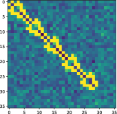
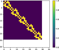
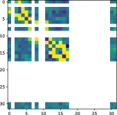
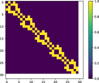
Figure 6: Probability of sampling each edge for state graph $\boldsymbol{\mathbf{h}}_{t}$. Node numbering is consistent with Figure 5. Nodes with index $\geq 30$ correspond to the extra nodes considered in $\mathbb{V}_{\boldsymbol{\mathbf{h}}}$ of eGSS.

5.3 Results

Table 2 shows that all graph-based models (i.e., gRNN, eGSS, and eGSS-in) achieve near-optimal MAE on GPVAR which corresponds to $0.319$ as derived analytically from the noise distribution. Instead, sRNN and fcRNN obtained substantially larger MAEs. These conclusions are also confirmed by the AZ-tests (Zambon and Alippi, 2022) assessing the presence of correlation in the prediction residuals which, in turn, is informative of whether the model can be considered optimal or not. The AZ-test statistics shows also that the sRNN was able to remove all temporal correlations from the data (see AZ-test temporal) but, as expected, residuals are substantially spatially correlated (see AZ-test spatial) as no information is exchanged between nodes. Conversely, fcRNN was able to account for the spatial correlations but not entirely for the temporal ones. On poGPVAR, the graph-based models are still the best-performing options, yet the AZ-test identifies the presence of some correlations left in the residuals, mostly ascribable to the spatial domain and, most likely, associated with the unobserved nodes.

Finally, regarding the graph-based models, we stress that eGSS is able to achieve performance comparable to gRNN and eGSS-in, even though eGSS does not have access to the ground-truth graph that generated the data. Figure 6 shows examples of learned graph topology which qualitatively matches the ground truth; for poGPVAR, we also observe that eGSS attempts to connect nodes 6, 8, and 11 [see Figure 5] which would allow passing information between the disconnected components. We conclude that our proposed framework is able to solve the task by effectively learning graph state representations capturing important relations underlying the observed time series.

6 Conclusions

We presented the first probabilistic state-space framework for modeling spatio-temporal data where inputs, states, and outputs are graphs. The proposed framework is general, allowing for learning graph states of variable topology directly from data, and several state-of-the-art methods are reinterpreted as special cases. The designed encoder-decoder architecture can be trained end-to-end and it is able to achieve optimal performance with no knowledge about the relational structure of the process generating the data.

Acknowledgements

This work was supported by the Swiss National Science Foundation project FNS 204061: High-Order Relations and Dynamics in Graph Neural Networks.

References

- Alippi [2014] Cesare Alippi. Intelligence for embedded systems, volume 89. Springer, 2014.
- Bacciu et al. [2020] Davide Bacciu, Federico Errica, Alessio Micheli, and Marco Podda. A gentle introduction to deep learning for graphs. Neural Networks, 2020.
- Bianchi et al. [2020] Filippo Maria Bianchi, Daniele Grattarola, and Cesare Alippi. Spectral clustering with graph neural networks for graph pooling. In International Conference on Machine Learning, pages 874–883. PMLR, 2020.
- Bronstein et al. [2017] Michael M Bronstein, Joan Bruna, Yann LeCun, Arthur Szlam, and Pierre Vandergheynst. Geometric deep learning: going beyond euclidean data. IEEE Signal Processing Magazine, 34(4):18–42, 2017.
- Bronstein et al. [2021] Michael M Bronstein, Joan Bruna, Taco Cohen, and Petar Veličković. Geometric deep learning: Grids, groups, graphs, geodesics, and gauges. arXiv preprint arXiv:2104.13478, 2021.
- Brunton et al. [2016] Steven L Brunton, Joshua L Proctor, and J Nathan Kutz. Discovering governing equations from data by sparse identification of nonlinear dynamical systems. Proceedings of the national academy of sciences, 113(15):3932–3937, 2016.
- Brunton et al. [2021] Steven L Brunton, Marko Budišić, Eurika Kaiser, and J Nathan Kutz. Modern koopman theory for dynamical systems. arXiv preprint arXiv:2102.12086, 2021.
- Chen et al. [2017] Badong Chen, Xi Liu, Haiquan Zhao, and Jose C Principe. Maximum correntropy kalman filter. Automatica, 76:70–77, 2017.
- Chen et al. [2022] Yakun Chen, Zihao Li, Chao Yang, Xianzhi Wang, Guodong Long, and Guandong Xu. Adaptive graph recurrent network for multivariate time series imputation. In International Conference on Neural Information Processing, 2022.
- Cini et al. [2020] Andrea Cini, Slobodan Lukovic, and Cesare Alippi. Cluster-based aggregate load forecasting with deep neural networks. In 2020 International Joint Conference on Neural Networks (IJCNN), pages 1–8. IEEE, 2020.
- Cini et al. [2021] Andrea Cini, Ivan Marisca, and Cesare Alippi. Filling the g_ap_s: Multivariate time series imputation by graph neural networks. In International Conference on Learning Representations, 2021.
- Cini et al. [2022] Andrea Cini, Daniele Zambon, and Cesare Alippi. Sparse graph learning for spatiotemporal time series, 2022. URL https://arxiv.org/abs/2205.13492.
- Coutino et al. [2020] Mario Coutino, Elvin Isufi, Takanori Maehara, and Geert Leus. State-space network topology identification from partial observations. IEEE Transactions on Signal and Information Processing over Networks, 6:211–225, 2020.
- Durbin and Koopman [2012] James Durbin and Siem Jan Koopman. Time series analysis by state space methods, volume 38. OUP Oxford, 2012.
- Gilmer et al. [2017] Justin Gilmer, Samuel S Schoenholz, Patrick F Riley, Oriol Vinyals, and George E Dahl. Neural message passing for quantum chemistry. In Proceedings of the 34th International Conference on Machine Learning-Volume 70, pages 1263–1272. JMLR. org, 2017.
- Grattarola et al. [2022] Daniele Grattarola, Daniele Zambon, Filippo Bianchi, and Cesare Alippi. Understanding pooling in graph neural networks. IEEE Transactions on Neural Networks and Learning Systems, pages 1–11, 2022. 10.1109/TNNLS.2022.3190922.
- Hochreiter and Schmidhuber [1997] Sepp Hochreiter and Jürgen Schmidhuber. Long short-term memory. Neural computation, 9(8):1735–1780, 1997.
- Kalman and Bucy [1961] Rudolph E Kalman and Richard S Bucy. New results in linear filtering and prediction theory. Journal of Basic Engineering, 83(1):95–108, 03 1961. ISSN 0021-9223. 10.1115/1.3658902. URL https://doi.org/10.1115/1.3658902.
- Kalman [1960] Rudolph Emil Kalman. A new approach to linear filtering and prediction problems. Journal of Basic Engineering, 82(1):35–45, 03 1960. ISSN 0021-9223. 10.1115/1.3662552. URL https://doi.org/10.1115/1.3662552.
- Kazemi et al. [2020] Seyed Mehran Kazemi, Rishab Goel, Kshitij Jain, Ivan Kobyzev, Akshay Sethi, Peter Forsyth, and Pascal Poupart. Representation learning for dynamic graphs: A survey. J. Mach. Learn. Res., 21(70):1–73, 2020.
- Kazi et al. [2022] Anees Kazi, Luca Cosmo, Seyed-Ahmad Ahmadi, Nassir Navab, and Michael Bronstein. Differentiable graph module (dgm) for graph convolutional networks. IEEE Transactions on Pattern Analysis and Machine Intelligence, 2022.
- Kipf et al. [2018] Thomas Kipf, Ethan Fetaya, Kuan-Chieh Wang, Max Welling, and Richard Zemel. Neural relational inference for interacting systems. In International Conference on Machine Learning, pages 2688–2697. PMLR, 2018.
- Li et al. [2018] Yaguang Li, Rose Yu, Cyrus Shahabi, and Yan Liu. Diffusion convolutional recurrent neural network: Data-driven traffic forecasting. In International Conference on Learning Representations, 2018. URL https://openreview.net/forum?id=SJiHXGWAZ.
- Marisca et al. [2022] Ivan Marisca, Andrea Cini, and Cesare Alippi. Learning to reconstruct missing data from spatiotemporal graphs with sparse observations. To appear in Advances in Neural Information Processing Systems, 2022.
- Mohamed et al. [2020] Shakir Mohamed, Mihaela Rosca, Michael Figurnov, and Andriy Mnih. Monte carlo gradient estimation in machine learning. Journal of Machine Learning Research, 21(132):1–62, 2020.
- Pal et al. [2021] Soumyasundar Pal, Liheng Ma, Yingxue Zhang, and Mark Coates. Rnn with particle flow for probabilistic spatio-temporal forecasting. In International Conference on Machine Learning, pages 8336–8348. PMLR, 2021.
- Salinas et al. [2020] David Salinas, Valentin Flunkert, Jan Gasthaus, and Tim Januschowski. Deepar: Probabilistic forecasting with autoregressive recurrent networks. International Journal of Forecasting, 36(3):1181–1191, 2020.
- Seo et al. [2018] Youngjoo Seo, Michaël Defferrard, Pierre Vandergheynst, and Xavier Bresson. Structured sequence modeling with graph convolutional recurrent networks. In International conference on neural information processing, pages 362–373. Springer, 2018.
- Stankovic et al. [2019] Ljubisa Stankovic, Danilo P Mandic, Milos Dakovic, Ilia Kisil, Ervin Sejdic, and Anthony G Constantinides. Understanding the basis of graph signal processing via an intuitive example-driven approach [lecture notes]. IEEE Signal Processing Magazine, 36(6):133–145, 2019.
- Trivedi et al. [2019] Rakshit Trivedi, Mehrdad Farajtabar, Prasenjeet Biswal, and Hongyuan Zha. Dyrep: Learning representations over dynamic graphs. In International Conference on Learning Representations, 2019. URL https://openreview.net/forum?id=HyePrhR5KX.
- Wang et al. [2019] Yuyang Wang, Alex Smola, Danielle Maddix, Jan Gasthaus, Dean Foster, and Tim Januschowski. Deep factors for forecasting. In International conference on machine learning, pages 6607–6617. PMLR, 2019.
- Wu et al. [2019] Z Wu, S Pan, G Long, J Jiang, and C Zhang. Graph wavenet for deep spatial-temporal graph modeling. In The 28th International Joint Conference on Artificial Intelligence (IJCAI). International Joint Conferences on Artificial Intelligence Organization, 2019.
- Ying et al. [2018] Zhitao Ying, Jiaxuan You, Christopher Morris, Xiang Ren, Will Hamilton, and Jure Leskovec. Hierarchical graph representation learning with differentiable pooling. In Advances in neural information processing systems, pages 4800–4810, 2018.
- Zambon and Alippi [2022] Daniele Zambon and Cesare Alippi. Az-whiteness test: a test for uncorrelated noise on spatio-temporal graphs, 2022. URL https://arxiv.org/abs/2204.11135.