Radiance Textures for Rasterizing Ray-Traced Data

Abstract.

Presenting real-time rendering of 3D surfaces using radiance textures for fast synthesis of complex incidence-variable effects and environment interactions. This includes iridescence, parallax occlusion and interior mapping, (specular, regular, diffuse, total-internal) reflections with many bounces, refraction, subsurface scattering, transparency, and possibly more. This method divides textures into a matrix of radiance buckets, where each bucket represent some data at various incidence angles. Data can show final pixel color, or deferred rendering ambient occlusion, reflections, shadow map, etc. Resolution of the final synthesized output is the radiance bucket matrix size. Technique can be implemented with a simple fragment shader. The computational footprint of this technique is of simple diffuse-only graphics, but with visual fidelity of complex (off-line) ray-traced render at the cost of storage memory footprint. Balance between computational footprint and storage memory footprint can be easily achieved with variable compression ratio of repetitive radiance scene textures.

© 2024 Jakub Maksymilian Fober

This work is licensed under Creative Commons BY-NC-ND 3.0 license. https://creativecommons.org/licenses/by-nc-nd/3.0/
For all other uses including commercial, contact the owner/author(s).

1. Introduction

Radiance and reflectance field rendering techniques are a class of algorithms used in computer graphics to generate images of three-dimensional scenes. These algorithms simulate the way light interacts with surfaces in a virtual environment, producing realistic and detailed images.

These techniques have been the subject of extensive research in computer graphics and rendering, as they offer a powerful and flexible way to generate high-quality images. There is a wide range of applications for radiance and reflectance field algorithms, including film and video game production, architectural visualization, and scientific visualization.

In this paper, technique is presented to capture and render complex precomputed light interactions, via radiance field textures, embedded onto three-dimensional-object’s surface.

The presented technique utilizes a standard fragment pixel shader and a two-dimensional texture lookup to render dynamic, view-independent, photo-realistic images at a fraction of the computational cost associated with effects such as real-time ray tracing, parallax mapping, and dynamic shadowing.

It is well-suited for real-time execution in video games, virtual reality, and virtual production environments on modern hardware. It can take advantage of the direct storage capability in ninth-generation gaming systems, providing high-fidelity, high-performance images.

This technique can replace computationally heavy rendering-pipeline chains, while preserving hardware-accelerated, highly-optimized rasterization elements. It can also enable wider implementation of real-time GPU ray-tracing, with ability to combine bounce rays with precomputed radiance of the environment.

1.1. Previous work

Mainstream implementations of radiance field rendering focus on volumetric data structures and spherical harmonics for rendering images(Yu et al., 2021). While volumetric data can be sparse in order to exclude void regions(Yu et al., 2021), the ultimate goal would logically be to perfectly match the geometry of the represented object. And since the inside volume of the object is of no interest (most of the time), only half of the radiance sphere is considered practically useful. Therefore, such fields could effectively be spread across the surface of the object.

Some researchers embraced this approach, with neural reflectance fields as texturing primitives(Baatz et al., 2022), which rendered high-fidelity results. But while neural fields produce fantastic results, they are computationally intensive at rendering time(Yu et al., 2021) and therefore are not suitable for real-time applications.

1.2. Overview of the content

In this initial version of paper you will find theoretical explanation and implementation of the subject, along with equations and schematics. Some elements had been tested, like mapping functions, some yet to be presented, as the follow-up updates continue.

1.3. Document naming convention

This document uses the following naming convention:

• Left-handed coordinate system.

• Vectors presented natively in column.

• Row-major order matrix arranged, denoted “$M_{\text{row}\,\text{col}}$”.

• Matrix multiplication by “$[\text{column}]_{a}\cdot[\text{row}]_{b}=M_{a\,b}$”.

• A single bar enclosure “$|u|$” represents scalar absolute.

• A single bar enclosure “$|\vec{v}|$” represents vector’s length.

• Vectors with an arithmetic sign, or without, are calculated component-wise and form another vector.

• Centered dot “$\cdot$” represents the vector dot product.

• Square brackets with a comma “$[f,c]$” denote interval.

• Square brackets with blanks “$[x\ y]$” denote vectors and matrices.

• The power of “^-1” implies the reciprocal of the value.

• QED symbol “$\square$” marks the final result or output.

This naming convention simplifies the process of transforming formulas into shader code.

2. Methodology

Each pixel of the model’s texture contains discrete radiance hemispherical map of size $n\times n$, called “bucket”. Buckets are arranged in place of initial texture’s pixels, increasing overall resolution to $w\cdot n\times h\cdot n$ pixels, where $w$ and $h$ denote width and height of the synthesized output texture, respectively. Buckets are highly repetitive and change only slightly from one to another. This is a great case for a simple compression.

To synthesize output texture for a given view position, single sample per bucket is taken, giving normal resolution texture output.

Model’s $u,v$ texture coordinates correspond to bucket matrix position index, while incidence vector, correspond to bucket’s internal $u,v$ position. Therefore radiance texture sampling algorithm can be described as a four-dimensional plenoptic function $L(u,v,\theta,\phi)$, where $u,v$ denote model’s texture coordinates and $\theta,\phi$ incidence angles.

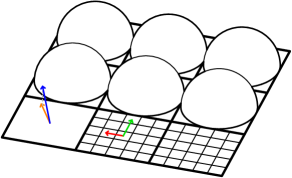
Figure 1. Radiance texture sampling model, where the incidence $\mathbb{R}^{3}$ vector (blue) is projected and squarified (orange) to $\mathbb{R}^{2}$ texture coordinates (red and green), which map onto hemispherical radiance bucket represented as a flat square.

Each radiance bucket should represent a hemisphere of reflectivity. Equisolid azimuthal projection was chosen for this task, for its properties, as it preserves area and resembles spherical mirror reflection(Wikipedia contributors, 2022). Resolution of the radiance bucket, in such projection, directly corresponds to $\sin(\nicefrac{{\theta}}{{2}})\sqrt{2}$, where $\theta$ is the incidence angle.

To efficiently spread information across square buckets, additional disc-to-square mapping function was implemented, providing uniform pixel count across both orthogonal directions and diagonal directions.

Equisolid azimuthal projection mapping can be easily implemented in the vector domain without the use of anti-trigonometric functions, as the orthographically projected normalized sum of the incidence and normal vectors has a length of $\sin(\nicefrac{{\theta}}{{2}})$. This eliminates $\theta,\phi$ angles from the plenoptic function, resulting in new $L^{\prime}(u,v,x,y,z)$, where $x,y,z$ correspond to incidence unit-vector components in orthogonal texture space.

2.1. Mapping of incident vector to radiance bucket

For every visible pixel there is an incidence vector $\hat{I}\in\mathbb{R}^{3}$. This vector can be mapped and projected to $\mathbb{R}^{2}$ texture coordinates using translation and $\mathbb{R}^{2\times 3}$-matrix transformation.

Following equation maps incidence vector to azimuthal equisolid projection, with $r=1$, at $\Omega=180\text{\textdegree}$.

(1a) $$\begin{bmatrix}\vec{A}_{x}\\ \vec{A}_{y}\\ \sqrt{2}\cos\nicefrac{{\theta}}{{2}}\end{bmatrix} =\sqrt{2}\left\|\begin{bmatrix}\hat{I}_{x}+\hat{N}_{x}\\ \hat{I}_{y}+\hat{N}_{y}\\ \hat{I}_{z}+\hat{N}_{z}\end{bmatrix}\right\|$$

(1b) $$\begin{bmatrix}\vec{A}_{x}\\ \vec{A}_{y}\end{bmatrix} =\frac{\sqrt{2}}{\left|\begin{bmatrix}\hat{I}_{x}&\hat{I}_{y}&\hat{I}_{z}+1\end{bmatrix}\right|}\begin{bmatrix}\hat{I}_{x}\\ \hat{I}_{y}\end{bmatrix} \text{, if }\hat{N}_{z}=1$$

Inverse mapping:

(2a) $$\begin{bmatrix}\hat{A}_{x}^{\prime}\\ \hat{A}_{y}^{\prime}\\ \hat{A}_{z}^{\prime}\end{bmatrix} =\begin{bmatrix}\vec{A}_{x}\sqrt{\nicefrac{{1}}{{2}}}\\ \vec{A}_{y}\sqrt{\nicefrac{{1}}{{2}}}\\ \sqrt{1-\frac{\vec{A}_{x}^{2}}{2}-\frac{\vec{A}_{y}^{2}}{2}}\end{bmatrix}$$

(2b) $$\begin{bmatrix}\hat{I}_{x}\\ \hat{I}_{y}\\ \hat{I}_{z}\end{bmatrix} =2\left(\hat{A}^{\prime}\cdot\hat{N}\begin{bmatrix}\hat{A}_{x}^{\prime}\\ \hat{A}_{y}^{\prime}\\ \hat{A}_{z}^{\prime}\end{bmatrix}-\begin{bmatrix}\hat{N}_{x}\\ \hat{N}_{y}\\ \hat{N}_{z}\end{bmatrix}\right)+\begin{bmatrix}\hat{N}_{x}\\ \hat{N}_{y}\\ \hat{N}_{z}\end{bmatrix}$$

(2c) $$=\begin{bmatrix}\vec{A}_{x}\sqrt{2-\vec{A}_{x}^{2}-\vec{A}_{y}^{2}}\\ \vec{A}_{y}\sqrt{2-\vec{A}_{x}^{2}-\vec{A}_{y}^{2}}\\ 1-\vec{A}_{x}^{2}-\vec{A}_{y}^{2}\end{bmatrix} \text{, if }\hat{N}_{z}=1$$

where $\vec{A}\in[-1,1]^{2}$ is the azimuthal equisolid projection coordinate. $\theta$ is the incidence angle. $\hat{N}\in\mathbb{R}^{3}$ is the surface normal vector. As the incidence $\hat{I}\in\mathbb{R}^{3}$ is mapped to or from orthogonal texture space, where $\hat{N}_{z}=1$, the transformation can take form of equation 1b and 2c.

Following equation transforms azimuthal projection vector, into square coordinates, for the radiance bucket sampling.

(3) $$\begin{bmatrix}\vec{B}_{x}\\ \vec{B}_{y}\end{bmatrix}=\frac{\big{|}\begin{bmatrix}\vec{A}_{x}&\vec{A}_{y}\end{bmatrix}\big{|}}{\max\big{(}|\vec{A}_{x}|,|\vec{A}_{y}|\big{)}}\begin{bmatrix}\vec{A}_{x}\\ \vec{A}_{y}\end{bmatrix}\quad\text{if }\vec{A}_{x}\text{ and }\vec{A}_{y}\neq 0\\$$

where $\vec{B}\in[-1,1]^{2}$ is the bucket’s centered texture coordinate and $\vec{A}\in[-1,1]^{2}$ is the azimuthal projection vector.

Note

It is important to prevent pixel blending between edges of neighboring buckets. This can be done by clamping bucket coordinates to $\vec{B}\in[B_{\textit{res}}^{-1}-1,1-B_{\textit{res}}^{-1}]^{2}$ range.

Inverse transformation of bucked, centered coordinates $\vec{B}\in\mathbb{R}^{2}$ to azimuthal projection coordinates $\hat{A}\in\mathbb{R}^{2}$ can be achieved with same, but inverted method.

(4a) $$\begin{bmatrix}\vec{A}_{x}\\ \vec{A}_{y}\end{bmatrix} =\frac{\max\big{(}|\vec{B}_{x}|,|\vec{B}_{y}|\big{)}}{\sqrt{\vec{B}_{x}^{2}+\vec{B}_{y}^{2}}}\begin{bmatrix}\vec{B}_{x}\\ \vec{B}_{y}\end{bmatrix}$$

(4b) $$\begin{bmatrix}\hat{R}_{x}\\ \hat{R}_{y}\\ \hat{R}_{z}\end{bmatrix} =\begin{bmatrix}-\vec{A}_{x}\sqrt{2-\vec{A}_{x}^{2}-\vec{A}_{y}^{2}}\\ -\vec{A}_{y}\sqrt{2-\vec{A}_{x}^{2}-\vec{A}_{y}^{2}}\\ 1-\vec{A}_{x}^{2}-\vec{A}_{y}^{2}\end{bmatrix}$$

where $\hat{R}\in\mathbb{R}^{3}$ denotes equisolid reflection vector. This vector is used to sample ray-traced data onto radiance field texture. It is a version of the vector mirrored along the normal, found in equation 2c.

(a) Picture of one cent American coin.

(b) One cent coin mapped to a rectangle, using equation 3.

Figure 2. A visual example of disc to square mapping using the formulation found in equation 3.

3. Results

TBA

4. Conclusion

I have theorized about possible implementation of radiance field texturing using modern hardware shading capabilities, and presented mathematical solution for executing such concept.

Note

More conclusion are to be added, after the update to the paper.

5. Possible applications

Radiance field texture sampling can replace shading pipeline or supplement it with enhanced effects. Some such effects include:

Parallax interior mapping

This effect is used to mimic interior of a room, as seen through a window, or it can simulate a portal to another place.

Proxy meshes with parallax mapping

Radiance texture with alpha mask can simulate more complex or furry objects bound inside a proxy mesh. Similarly to neural radiance fields texturing primitives(Baatz et al., 2022).

Reflections

Many light bounces can be combined into a single pixel of the radiance texture map. Dynamic objects can then sample such radiance field to obtain environment reflections. Also semi real-time ray-tracing can accumulate dynamically generated reflections into such texture map, to update and enhance environment one.

Shadowing

1-bit radiance field texture map can represent shadowing of static objects. Here, incidence vector is replaced with light direction vector for shadow occlusion sampling. It can work with both parallel light sources and point lights. With more than one sample per bucket, area shadows are possible to produce.

Subsurface scattering

This computationally demanding effect can be encoded in a radiance texture map, which then replaces incidence vector, with the light direction vector in relation to the view position for sampling.

References

- (1)
- Baatz et al. (2022) H. Baatz, J. Granskog, M. Papas, F. Rousselle, and J. Novák. 2022. NeRF-Tex: Neural Reflectance Field Textures. Computer Graphics Forum 41, 6 (March 2022), 287–301. https://doi.org/10.1111/cgf.14449
- Wikipedia contributors (2022) Wikipedia contributors. 2022. Fisheye lens: Mapping function. Wikipedia, The Free Encyclopedia. https://en.wikipedia.org/w/index.php?title=Fisheye_lens&oldid=1124809304#Mapping_function [Online].
- Yu et al. (2021) Alex Yu, Sara Fridovich-Keil, Matthew Tancik, Qinhong Chen, Benjamin Recht, and Angjoo Kanazawa. 2021. Plenoxels: Radiance Fields without Neural Networks. arXiv (Dec. 2021). https://doi.org/10.48550/ARXIV.2112.05131