Spectral analysis and $k$-spine decomposition of inhomogeneous branching Brownian motions. Genealogies in fully pushed fronts

Abstract

We consider a system of particles performing a one-dimensional dyadic branching Brownian motion with space-dependent branching rate, negative drift $-\mu$ and killed upon reaching $0$. More precisely, the particles branch at rate $r(x)=(1+W(x))/2,$ where $W$ is a compactly supported and non-negative smooth function and the drift $\mu$ is chosen in such a way that the system is critical in some sense.

This particle system can be seen as an analytically tractable model for fluctuating fronts, describing the internal mechanisms driving the invasion of a habitat by a cooperating population. Recent studies from Birzu, Hallatschek and Korolev suggest the existence of three classes of fluctuating fronts: pulled, semi pushed and fully pushed fronts. Here, we focus on the fully pushed regime. We establish a Yaglom law for this branching process and prove that the genealogy of the particles converges to a Brownian Coalescent Point Process using a method of moments.

In practice, the genealogy of the BBM is seen as a random marked metric measure space and we use spinal decomposition to prove its convergence in the Gromov-weak topology. We also carry the spectral decomposition of a differential operator related to the BBM to determine the invariant measure of the spine as well as its mixing time.

1 Introduction

1.1 The model and assumptions

We consider a dyadic branching Brownian motion $(\mathbf{X}_{t})_{t>0}$ (BBM) with killing at $0$, negative drift $-\mu$ and position-dependent branching rate

$$r(x)=\frac{1}{2}W(x)+\frac{1}{2},$$ (1)

for some function $W:[0,+\infty)\rightarrow\mathbb{R}$. We assume that $W$ satisfies the following assumptions:

• the function $W$ is non-negative, continuously differentiable and compactly supported.

• the support of $W$ is included in $[0,1]$.

We denote by $\mathcal{N}_{t}$ the set of particles in the system at time $t$ and for all $v\in\mathcal{N}_{t}$, we denote by $x_{v}=x_{v}(t)$ the position of the particle $v$. Furthermore, we write $Z_{t}:=|{\cal N}_{t}|$ for the number of particles in the system at time $t$. We write $\mathbb{P}_{x}$ for the law of the process initiated from a point $x\geq 0$ and $\mathbb{E}_{x}$ for the corresponding expectation.

Critical regime. We aim at choosing $\mu$ in such a way that the number of particles in the system stays roughly constant.

Fix $L>1$ and consider the BBM $(\mathbf{X}^{L}_{t})_{t>0}$ with branching rate $r(x)$, drift $-\mu$ and killed at $0$ and $L$. Denote by $\mathcal{N}_{t}^{L}$ the set of particles in this system at time $t$ and define $Z^{L}_{t}=|\mathcal{N}_{t}^{L}|$. By a slight abuse of notations, we will also denote by $x_{v}$ the positions of the particles in the BBM $\mathbf{X}^{L}$. Let $(t,x,y)\mapsto p_{t}(x,y)$ be the fundamental solution of the linear equation

$$\begin{cases}\partial_{t}u(t,y)=\frac{1}{2}\partial_{yy}u(t,y)+\mu\partial_{y}u(t,y)+r(y)u(t,y)\\ u(t,0)=u(t,L)=0.\end{cases}$$ (A)

We say that $p_{t}\equiv p_{t}^{L}$ is the density of particles in $\mathbf{X}^{L}$ in the sense that for any measurable set $B\subset[0,L]$, the expected number of particles in $B$ at time $t$ starting from a single particle at $x$ is given by $\int_{B}p_{t}(x,y)dy$ [Law18, p.188]. Let us now define

$${g}_{t}(x,y):=e^{\mu(y-x)}e^{\frac{\mu^{2}-1}{2}t}p_{t}(x,y).$$ (2)

A direct computation shows that $g_{t}$ is the fundamental solution of the self-adjoint PDE

$$\begin{cases}\partial_{t}u(t,y)=\frac{1}{2}\partial_{yy}u(t,y)+\frac{1}{2}W(y)u(t,y)\\ u(t,0)=u(t,L)=0.\end{cases}$$ (B)

Let $\lambda_{1}=\lambda_{1}(L)$ be the maximal eigenvalue [Zet12, Chapter 4] of the Sturm–Liouville problem

$$\frac{1}{2}v^{\prime\prime}(x)+\frac{1}{2}W(x)v(x)=\lambda v(x),$$ (SLP)

with boundary conditions

$$v(0)=v(L)=0.$$ (BC)

It is known that $\lambda_{1}$ is an increasing function of $L$ [Pin95, Theorem 4.4.1] and that it converges to a finite limit $\lambda_{1}^{\infty}\in(-\infty,+\infty)$ as $L\to\infty$ [Pin95, Theorem 4.3.2]. We now choose $\mu$ in such a way that the expected number of particles is neither increasing nor decreasing exponentially. According to (2), we expect that for large $t$

$$p_{t}(x,y)\approx e^{\mu(x-y)}e^{\frac{1-\mu^{2}}{2}t}e^{\lambda_{1}^{\infty}t}\frac{v_{1}(x)v_{1}(y)}{||v_{1}||^{2}},$$

where $v_{1}$ denotes an eigenfunction associated to $\lambda_{1}$ for the Sturm–Liouville problem (SLP). This motivates the following definition.

Definition 1 (Critical regime).

The BBM is in the critical regime iff

$$\mu=\sqrt{1+2\lambda_{1}^{\infty}}.$$ (3)

Pushed and pulled waves. The next definitions are motivated by recent numerical simulations and heuristics [BHK18, BHK21] for the noisy F-KPP equation with Allee effect

$$u_{t}=\frac{1}{2}u_{xx}+u(1-u)(1+Bu)+\sqrt{\frac{u}{N}}{\eta},$$

where $B>0$, $N$ is a large demographic parameter and $\eta$ is a space-time white noise. See [Tou21] for more details and [EP22] for recent rigorous results on the bistable case.

Definition 2 (Pulled, semi pushed, fully pushed regimes).

Consider the BBM $(\mathbf{X}_{t})$ in the critical regime. Define

$$\beta:=\sqrt{2\lambda_{1}^{\infty}},\quad\text{and}\quad\alpha:=\frac{\mu+\beta}{\mu-\beta}.$$ (4)

1. If $\lambda_{1}^{\infty}=0$, or equivalently $\alpha=1$, the BBM is said to be pulled.

2. If $\lambda_{1}^{\infty}\in(0,1/16)$ or equivalently

   $$\alpha\in(1,2)\Longleftrightarrow\mu>3\beta,$$

   the BBM is said to be semi pushed.

3. If $\lambda_{1}^{\infty}>1/16$ or equivalently

   $$\alpha>2\Longleftrightarrow\mu<3\beta, H_{fp}$$ ()

   the BBM is said to be fully pushed.

We say that the BBM is pushed if it is either semi or fully pushed, that is when

$$\lambda_{1}^{\infty}>0. H_{p}$$ ()

Example 1.1.

Let $\varepsilon>0$ and consider the BBM with inhomogeneous branching rate $r_{\varepsilon}(x)=\frac{1}{2}+\varepsilon W(x)$. By [Pin95, Theorem 4.6.4 and Theorem 4.4.3], for any function $W$ satisfying (A1), there exists $0<\varepsilon_{1}<\varepsilon_{2}$ such that

1. The BBM is pulled for all $\varepsilon\in(0,\varepsilon_{1})$.

2. The BBM is semi pushed for all $\varepsilon\in(\varepsilon_{1},\varepsilon_{2})$.

3. The BBM is fully pushed for all $\varepsilon>\varepsilon_{2}$.

It is conjectured that up to rescaling, the size and the genealogy at large time is undistinguishable from the ones of a continuous-state branching process (CSBP). More precisely,

1. In the pulled regime, the population size should converge to a Neveu’s continuous-state branching process and the genealogy of the BBM to the Bolthausen–Sznitman coalescent (see [BBS13] in the case $W\equiv 0$).

2. In the semi pushed regime, the population size should converge to an $\alpha$-stable CSBP. In the previous example, this has been proved only in the case where $W=1_{[0,1]}$ [Tou21]. Therein, it is also conjectured that the genealogy should converge to a time-changed $\mbox{Beta}(\alpha,2-\alpha)$ coalescent [Pit99, Sag99, BBC⁺05].

3. In the fully pushed regime, the rescaled population size should converge to a Feller diffusion and the genealogy should be undistinguishable from the genealogy of a large critical Galton-Watson process with finite second moment. This is the content of the present article.

1.2 Comparaison with previous work

Branching Brownian motion with inhomogeneous branching rates have received quite a lot of attention in the recent past [HKV20, HHK20, HHKW22, GHK22, FRS22, Tou21, RS21, LS21]. The general approach always relies on a spinal decomposition of the BBM. Roughly speaking, the spine is constructed by conditioning a typical particle to survive. This conditioning is achieved by a Doob-$h$ transform. In our setting, the harmonic function is approximated by $h(x)\approx e^{\mu x}v_{1}(x)$ and the resulting $h$-transform is given by

$$dx_{t}=\frac{v_{1}^{\prime}(x_{t})}{v_{1}{(x_{t})}}dt\ +\ dB_{t}$$ (5)

where $B_{t}$ is a standard Brownian motion. See Section 3 for more details.

A key assumption underlying [Pow19, HKV20, HHK20, HHKW22, GHK22] is that the harmonic function $h$ is bounded. From a technical stand point, we emphasise that this assumption is the one distinguishing our work from the previous ones. Indeed, we shall see that $v_{1}$ decreases exponentially at rate $\beta$ so that the harmonic function $h(x)\propto e^{(\mu-\beta)x}$ blows up as $x$ tends to $\infty$. Due to the explosion of the harmonic function, many of the previously developed technics break down in our case.

At first sight, this assumption may only seem technical. However, it is the key assumption which makes possible a transition from the semi to the fully pushed regime. Let us consider the spine dynamics (5). In the pushed regime, the invariant distribution for the spine is given by

$$\Pi(x)=\frac{v_{1}^{2}(x)}{||v_{1}||^{2}}.$$ (6)

Hence, for $x$ large enough,

$$h(x)\Pi(x)\approx e^{(\mu-3\beta)x}.$$ (7)

It then becomes clear from Definition 2 that, in the fully pushed regime (resp. semi pushed), the harmonic function is integrable (resp. non-integrable) with respect to the invariant measure of the spine. As a consequence, relaxing the assumption under which $h$ is bounded is crucial for understanding the transition between these two regimes. This integrability condition already appeared in different forms in the literature:

• The harmonic function $h(x)$ can also be seen as the reproductive value of an individual at $x$, that is, its relative contribution to the travelling wave. Interestingly enough, this quantity also appears in the context of deterministic bistable fronts, see e.g. [RGHK12, Equations 8 and 9]. From this perspective, the variance in the offspring distribution of the BBM is given by

  $$\int_{0}^{\infty}r(y)p_{t}(x,y)h(y)^{2}dy.$$ (8)

  We see that (8) is finite when (7) is integrable. In addition, the Kolmogorov estimate and the Yaglom law established in this article are very similar to the one obtained in classical theory of multi-types Galton-Watson processes with finite variance [AN72, p.185] (see Section 1.3).

• In [EP22, BHK18], this integral is related to the rate of coalescence of the lineages at the tip of the front. As a first approximation, the lineages coalesce instantaneously when they meet on the same site so that the time to coalescence is roughly given by an exponential random variable of parameter proportional to

  $$\int_{0}^{\infty}\frac{1}{p_{t}(x,y)}r(y)\Pi(y)^{2}dy.$$ (9)

  When this parameter is finite, the genealogy of the sample should converge, after suitable scaling, to a Kingman coalescent. We will show that, for sufficiently large time $t$, the density of particles in the process $p_{t}(x,y)$ is roughly proportional to $e^{-2\mu y}h(y)=e^{-\mu y}v_{1}(y)$. As a consequence, the parameter (9) is finite precisely when (7) is integrable.

This generalisation raises interesting technical challenges. A large fraction of the present work (Section 4.1) is dedicated to estimating the speed of convergence of the spine to its invariant measure in the pushed regime. More precisely, we use a Sturm–Liouville approach in order to understand the spectral decomposition of the differential operator (B). The difficulty arises from the fact that the negative part of the spectrum of the Sturm–Liouville problem (SLP) becomes continuous as $L\to\infty$ (see Figure 1). We believe that this contribution is relevant for understanding not only the fully pushed regime, but also the semi pushed one, which will be the subject of future work. This continuous spectrum already appeared in the study of homogeneous BBM [BBS13], but the spectral analysis of (SLP) is quite straightforward in this case. Indeed, when $W\equiv 0$, the spectral decomposition is given by $\lambda_{i}=-\frac{i\pi^{2}}{2L^{2}}$ and $v_{i}(x)=\sin\left(\frac{i\pi x}{L}\right)$. When $W$ is not trivial, the spectrum is not explicit and we use the Prüfer transformation to derive the required estimates on the $(v_{i})$ and the $(\lambda_{i})$.

Finally, one of the main contribution of the present work is the description of the genealogy spanned by the population at a large time horizon. Beyond our Kolmogorov estimate and the Yaglom law reminiscent of [Pow19, HKV20, HHK20, HHKW22, GHK22], we use $k$-spine decompositions [HR17] and moment methods developed in [FRS22] to prove convergence of the genealogy in the Gromov weak topology to a continuum random metric space known as the Brownian Coalescent Point Process [Pop04]. This approach will be further explained in the next section.

Example 1.2.

Consider $W=10.\mathbb{1}_{[0,1]}$. It was calculated in [Tou21] that the negative part of the spectrum of (SLP) with boundary conditions (BC) consists in the solutions of

$$\frac{\tan(\sqrt{9-2\lambda})}{\sqrt{9-2\lambda}}=-\frac{\tan(\sqrt{-2\lambda}(L-1))}{\sqrt{-2\lambda}}.$$ (10)

The solutions of this equation are plotted on Figure 1

Figure 1: Negative spectrum of the Sturm–Liouville problem (SLP) with boundary conditions (BC) for $W$ defined as in Example 1.2 and different values of $L$. The blue line corresponds to RHS of (10) and the red line to the LHS of (10).

1.3 Main results

Proposition 1.3.

Let $v_{1}$ be the eigenfunction associated to the eigenvalue $\lambda_{1}$ for the Sturm–Liouville problem (SLP) with boundary conditions (BC), normalised in such a way that $v_{1}(1)=1$. Under ($H_{p}$), $v_{1}$ converges pointwise and in $\mathrm{L}^{2}$ to a positive limiting function $v_{1}^{\infty}$ as $L\to\infty$. Further, if in addition ($H_{fp}$) holds, then

$$\int_{\mathbb{R}_{+}}e^{\mu x}(v_{1}^{\infty})^{3}(x)dx<\infty.$$

To see why the latter proposition may hold true, recall that $W\equiv 0$ on $[1,\infty)$. Hence, on this interval, the problem reduces to

$$\quad\frac{1}{2}v_{1}^{\prime\prime}(x)=\lambda v_{1}(x),\quad x\in[1,L],\quad\ \ v_{1}(L)=0.$$

If we impose the condition $v_{1}(1)=1$, a direct computation shows that $v_{1}(x)=\frac{\sinh(\sqrt{2\lambda_{1}}(L-x))}{\sinh(\sqrt{2\lambda_{1}}(L-1))}$ on $[1,L]$ so that, for all $x\in[1,\infty)$, $v_{1}(x)\to v_{1}^{\infty}(x)=e^{-\beta(x-1)}$. The integrability condition then holds under the extra assumption ($H_{fp}$).

In the following, we define

$$\tilde{h}^{\infty}(x):=\tilde{c}e^{-\mu x}v_{1}^{\infty}(x),\quad\text{and}\quad h^{\infty}(x):=\frac{1}{\tilde{c}\|v_{1}^{\infty}\|^{2}}e^{\mu x}v_{1}^{\infty}(x),$$ (11)

where

$$\tilde{c}:=\left(\int_{0}^{\infty}e^{-\mu x}v_{1}^{\infty}(x)dx\right)^{-1}.$$

The constant $\tilde{c}$ is thought as a Perron-Frobenius renormalisation constant (see e.g. [AN72, p.185]), in the sense that $h^{\infty}$ (resp. $\tilde{h}^{\infty}$) is a right (resp. left) eigenfunction associated to the maximal eigenvalue of the differential operator

$$\mathcal{L}u=\frac{1}{2}\partial_{xx}u-\mu\partial_{x}u+r(x)u,$$ (12)

normalised in such a way that

$$\int_{0}^{\infty}\tilde{h}^{\infty}(x)dx=1\quad\text{and}\quad\int_{0}^{\infty}h^{\infty}(x)\tilde{h}^{\infty}(x)dx=1.$$

From this perspective, the function $\tilde{h}^{\infty}$ should correspond to the stable configuration of the system and the function $h^{\infty}$ to the reproductive values of the individuals as a function of their positions.

Theorem 1 (Kolmogorov estimate).

As $N\to\infty$, for all $x,t>0$,

$${N}\mathbb{P}_{x}\left(Z_{tN}>0\right)\to\frac{2}{\Sigma^{2}t}h^{\infty}(x),\ \ \mbox{where}\quad\frac{\Sigma^{2}}{2}\ :=\ \int_{\mathbb{R}_{+}}r(z)(h^{\infty}(z))^{2}\tilde{h}^{\infty}(z)dz.$$

This theorem is a continuous analogous of Kolmogorov estimate for multi-type Galton-Watson process [AN72, p.187].

We now turn to the description of the genealogy and the Yaglom law. Intuitively, the next result states that the genealogy is asymptotically identical to the one of a critical Galton Watson [Lam18, HJR20, Joh19], whereas the marks are assigned independently according to $\tilde{h}^{\infty}$. Let us now give a more precise description of our result.

From now on, we condition on the event $\{Z_{tN}>0\}$. Let $(v_{1},\dots,v_{k})$ be $k$ individuals chosen uniformly at random from ${\cal N}_{tN}$. Denote by $d_{T}(v_{i},v_{j})$ the time to the most recent common ancestor of $v_{i}$ and $v_{j}$. Let $x_{v_{i}}$ be the position of the $i^{th}$ individual at time $tN$.

Let $U$ be a uniform r.v. on $[0,t]$ and $\theta>0$. Define $U^{\theta}$ such that

$$\forall s\leq t,\qquad\mathbb{P}(U^{\theta}\leq s):=\frac{(1+\theta)\mathbb{P}(U\leq s)}{1+\theta\mathbb{P}(U\leq s)}.$$ (13)

Let $(U^{\theta}_{i};i\in[k])$ be $k$ i.i.d. copies of $U^{\theta}$ and set

$$\forall 1\leq i<j\leq k,\quad U^{\theta}_{i,j}=U^{\theta}_{j,i}:=\max\{U^{\theta}_{k}:k\in\{i,\cdots,j-1\}\}.$$

Finally, define the random distance matrix $(H_{i,j}):=(H_{i,j};i\neq j\in[k])$ such that for every bounded and continuous function $\varphi:\mathbb{R}^{k^{2}}\to\mathbb{R}$,

$$\mathbb{E}\big{[}\varphi\big{(}(H_{i,j})\big{)}\big{]}=k\int_{0}^{\infty}\frac{1}{(1+\theta)^{2}}\Big{(}\frac{\theta}{1+\theta}\Big{)}^{k-1}\mathbb{E}\big{[}\varphi\big{(}(U^{\theta}_{i,j})\big{)}\big{]}d\theta.$$ (14)

Finally, $(w_{i}):=(W_{i};i\in[k])$ will denote a sequence of i.i.d. copies of a random variable $w$ with law $\tilde{h}^{\infty}$.

Theorem 2 (Yaglom law and limiting genealogies).

Let $t>0$. Start with a single particle at $x>0$. Conditional on $Z_{tN}>0$, as $N\to\infty$,

1. we have

   $$\frac{Z_{tN}}{N}\to\frac{\Sigma^{2}t}{2}\ \mathcal{E},\ \ \ \mbox{in distribution,}$$

   where $\mathcal{E}$ is a standard exponential distribution.

2. $\left(\big{(}\tfrac{d_{T}(v_{i},v_{j})}{N}\big{)},\big{(}x_{v_{i}}\big{)}\right)$ converges to the distribution of $\left((H_{\sigma_{i},\sigma_{j}}),(W_{\sigma_{i}})\right)$ where $\sigma$ is a random uniform permutation $\{1,\dots,k\}$ and $\sigma$, $(H_{i,j})$ and $(w_{i})$ are independent.

Remark 1.4.

The random distance matrix $(H_{i,j})$ is the one obtained from a critical Galton Watson with finite second moment conditioned on surviving up to a large time. See [Lam18, HJR20, Joh19].

1.4 Notation

Given two sequences of positive real numbers $(a_{N})$ and $(b_{N})$, we write $a_{N}\ll b_{n}$ if $a_{N}/b_{N}\to 0$ as $N\to\infty$. We write $a_{N}\lesssim b_{N}$ if $a_{N}/b_{N}$ is bounded in absolute value by a positive constant and $a_{N}\asymp b_{N}$ if $a_{N}\lesssim b_{N}$ and $b_{N}\lesssim a_{N}$. We write $O(\cdot)$ to refer to a quantity bounded in absolute value by a constant times what the quantity inside the parentheses. Unless otherwise specified, these constants only depend on $\lambda_{1}^{\infty}$.

2 Outline of the proof

Our approach relies on a method of moments devised in [FRS22]. To illustrate the approach, let us first think about the Yaglom law of Theorem 2. To prove this result, one needs to show that the moments of $Z_{tN}/N$ converge to the moments of an exponential. It turns out that this approach can be extended to genealogies.

In Section 2.1, following the approach in [DGP11], we encode the genealogy at time $tN$ as a random marked measured metric space (mmm). The moments of a random mmm are obtained by biasing the population by its $k^{\text{th}}$ moment and then picking $k$ individuals uniformly at random (see Remark 2.1 below). In section 2.2, we introduce a limiting random mmm called the marked Coalescent Point Process (CPP) which corresponds to the limiting genealogy of a critical Galton-Watson process [Pop04]. The remainder of the section is dedicated to the sketch of the proof for the convergence of the moments of our BBM to the moments of the marked CPP using the spinal decomposition introduced in [FRS22].

2.1 Marked Metric Spaces

Let $(E,d_{E})$ be a fixed complete separable metric space, referred to as the mark space. In our application, $E=(0,\infty)$ is endowed with the usual distance on the real line. A marked metric measure space (mmm-space for short) is a triple $[X,d,\nu]$, where $(X,d)$ is a complete separable metric space, and $\nu$ is a finite measure on $X\times E$. We define $|X|:=\nu(X\times E)$. (Note that $\nu$ is not necessarily a probability distribution.) To define a topology on the set of mmm-spaces, for each $k\geq 1$, we consider the map

$$R_{k}\colon\begin{cases}(X\times E)^{k}\to\mathbb{R}_{+}^{k^{2}}\times E^{k}\\ \big{(}(x_{i},u_{i});\,i\leq k\big{)}\mapsto\big{(}d(x_{i},x_{j}),u_{i};\,i,j\leq k\big{)}\end{cases}$$

that maps $k$ points in $X\times E$ to the matrix of pairwise distances and marks. We denote by $\nu_{k,X}=\nu^{\otimes k}\circ R_{k}^{-1}$, the marked distance matrix distribution of $[X,d,\nu]$, which is the pushforward of $\nu^{\otimes k}$ by the map $R_{k}$. Let $k\geq 1$ and consider a continuous bounded test function $\varphi\colon\mathbb{R}_{+}^{k^{2}}\times E^{k}\to\mathbb{R}$. One can define a functional

$$\Phi\big{(}X,d,\nu\big{)}=\left<\nu_{k,X},\varphi\right>=\int_{X\times E}\varphi\bigg{(}d(v_{i},v_{j}),x_{i};i\neq j\in[k]\bigg{)}\prod_{i=1}^{k}\nu(dv_{i}\otimes dx_{i}).$$ (15)

Functionals of the previous form are called polynomials, and the set of all polynomials, obtained by varying $k$ and $\varphi$, is denoted by $\mathbf{\Pi}$. Finally, the moment of $[X,d,\mu]$ associated to $\Phi$ is defined as $\mathbb{E}(\Phi\big{(}X,d,\nu\big{)})$.

Let $\varphi$ be of the form

$$\varphi\bigg{(}d_{i,j},x_{i};i\neq j\in[k]\bigg{)}\ =\ \prod_{i,j}\psi_{i,j}(d_{i,j})\prod_{i}\varphi_{i}(x_{i}),$$

where $\psi_{i,j},\varphi_{i}$ are bounded continuous functions. We say that $\Phi(X,d,\nu)$ is a product polynomial. We denote by $\tilde{\mathbf{\Pi}}$ the set of product polynomials.

Remark 2.1.

Consider a random mmm $[X,d,\nu]$. Assume that $\mathbb{E}(|X|^{k})<\infty$. The moments of a random mmm can be rewritten as

$$\mathbb{E}\left(\Phi\big{(}X,d,\nu\big{)}\right)\ =\mathbb{E}(|X|^{k})\times\frac{1}{\mathbb{E}(|X|^{k})}\mathbb{E}\left(|X|^{k}\varphi(d(v_{i},v_{j}),X_{v_{i}},i\neq j\in[k])\right),$$

where $(v_{i},X_{v_{i}})$ are $k$ points sampled uniformly at random with their marks and $|X|:=\nu(X\times E)$ is thought as the total size of the population. As a consequence, the moments of a random mmm are obtained by biasing the population size by its $k^{th}$ moment and then picking $k$ individuals uniformly at random.

Definition 3.

The marked Gromov-weak (MGW) topology is the topology on mmm-spaces induced by $\mathbf{\Pi}$. A random mmm-space is a r.v. with values in $\mathbb{M}$ – the set of (equivalence classes of) mmm-spaces – endowed with the Gromov-weak topology and the associated Borel $\sigma$-field.

Finally, the marked Gromov-weak (MGW) topology is identical to the topology induced by the product polynomials $\tilde{\mathbf{\Pi}}$.

Many properties of the marked Gromov-weak topology are derived in [DGP11] under the further assumption that $\nu$ is a probability measure. In particular, the following result shows that $\mathbf{\Pi}$ forms a convergence determining class only when the limit satisfies a moment condition, which is a well-known criterion for a real variable to be identified by its moments, see for instance [Dur19, Theorem 3.3.25]. This result was already stated for metric measure spaces without marks in [DG19, Lemma 2.7] and was proved in [FRS22].

Proposition 2.2.

Suppose that $[X,d,\nu]$ is a random mmm-space verifying

$$\limsup_{p\to\infty}\frac{\mathbb{E}[|X|^{p}]^{1/p}}{p}<\infty.$$ (16)

Then, for a sequence $[X_{n},d_{n},\nu_{n}]$ of random mmm-spaces to converge in distribution for the marked Gromov-weak topology to $[X,d,\nu]$ it is sufficient that

$$\lim_{n\to\infty}\mathbb{E}\big{[}\Phi\big{(}X_{n},d_{n},\nu_{n}\big{)}\big{]}=\mathbb{E}\big{[}\Phi\big{(}X,d,\nu\big{)}\big{]}$$

for all $\Phi\in\mathbf{\Pi}$.

2.2 Marked Brownian Coalescent Point Process (CPP)

Let $T>0$ and $m$ be a measure on $\mathbb{R}_{+}$. Assume that $|m|:=m(\mathbb{R}_{+})>0$. Consider ${\cal P}$ a $PPP\left(\frac{dx}{x^{2}}\otimes dt\right)$. Define

$$Y_{T}\ =\ \inf\left\{y:(y,t)\in{\cal P},t\geq T\right\},$$

and

$$d_{T}(x,y)\ =\ \sup\{t\ :\ (z,t)\in{\cal P}\ \ \mbox{and}\ \ x\leq z\leq y\},\quad 0<x<y<Y_{T}.$$

The marked Brownian Coalescent Point Process (CPP) is defined as

$$M_{T}\ :=\ \bigg{(}[0,Y_{T}],d_{T},dv\otimes m(dx)\bigg{)}.$$

This object is a natural extension of the standard Brownian CPP [Pop04].

Remark 2.3.

A direct computation shows that $Y_{T}m(\mathbb{R}_{+})$ (which can be thought as the population size at time $T$) is distributed as an exponential random variable with mean $T|m|$. If the CPP encodes the size and the genealogy of critical branching processes, this consistent with Yaglom’s law for critical branching processes.

Figure 2: Simulation of the unmarked Brownian CPP. On the RHS, a vertical line of height $x$ at location $s$ represents an atom $(x,s)$ of $\cal{P}$. On the LHS, the tree corresponding to the right CPP; the distance $d_{T}$ is the tree distance of the leaves.

Proposition 2.4.

Let $K\in{\mathbb{N}}$. Let $(\varphi_{i};i\in[K])$ and $(\psi_{i,j};i,j\in[K])$ be measurable bounded functions. Consider an arbitrary product polynomial of the form

$$\forall M=[X,d,\nu],\ \ \Psi(M)\ :=\ \int\prod_{i,j}\psi_{i,j}(d_{T}({v_{i},v_{j}}))\prod_{i}\varphi_{i}(x_{i})\nu(dv_{i}\otimes dx_{i}).$$

Then

$$\mathbb{E}\left[\Psi(M_{T})\right]\ =\ K!T^{K}\mathbb{E}\left[\prod_{i,j}\psi_{i,j}(U_{\sigma_{i},\sigma_{j}})\right]\left[\prod_{i}\int m(dx)\varphi_{i}(x)\right]^{K},$$

where $(U_{i};i\in[K-1])$ is a vector of uniform i.i.d. random variables on $[0,T]$ and for $i<j$

$$U_{i,j}=U_{j,i}=\max\{U_{k}:k=i,\cdots,j-1\}.$$

Proof.

The proof is identical to Proposition 4 in [FRS22]. ∎

Proposition 2.5 (Sampling from the CPP).

Let $k\in\mathbb{N}$ and sample $k$ points $((v_{1},x_{1}),\cdots,(v_{k},x_{k})$ uniformly at random from the CPP. Then $(\left(d(v_{i},v_{j})\right)_{i,j},(x_{i})_{i})$ is identical in law to $\left((H_{\sigma_{i},\sigma_{j}}),(w_{\sigma_{i}})\right)$ where $(H_{i,j})$ is defined as in Theorem 2 (ii) and $(w_{i})$ are independent random variables with law $\frac{m}{|m|}$.

Proof.

The proof is identical to the one in the case of the unmarked CPP. See [BFRS22, Proposition 4.3]. ∎

2.3 Convergence of mmm

Fix $t>0$. Recall that ${\cal N}_{t}$ refers the set of particles alive at time $t$ in the BBM $\mathbf{X}$. Set

$$\nu_{t}\ :=\sum_{v\in{\cal N}_{t}}\delta_{v,x_{v}},\ \ \forall v,v^{\prime}\in{\cal N}_{t},\ \ d(v,v^{\prime})=\ t-|v\wedge v^{\prime}|,$$

where $v\wedge v^{\prime}$ denotes the MRCA of $v$ and $v^{\prime}$, and $|v|$ denotes the generation of vertex $v$. Let $M_{t}=[{\cal N}_{t},d,\nu_{t}]$ be the resulting random mmm. Finally, set

$$\bar{\nu}_{t}\ :=\ \frac{1}{N}\sum_{v\in{\cal N}_{tN}}\delta_{v,x_{v}},\ \ \forall v,v^{\prime}\in{\cal N}_{tN},\ \ \bar{d}(v,v^{\prime})=\ \left(t-\frac{1}{N}|v\wedge v^{\prime}|\right),$$

and define the rescaled metric space $\bar{M}_{t}\ :=\ [{\cal N}_{tN},\bar{d},\bar{\nu}_{t}]$. The main idea underlying Theorem 2 is to prove the convergence of $\bar{M}_{t}$ to a limiting CPP.

Theorem 3.

Conditional on the event $\{Z_{tN}>0\}$, $(\bar{M}_{t};N\in\mathbb{N})$ converges in distribution to a marked Brownian CPP with parameters $(t,\frac{\Sigma^{2}}{2}\tilde{h}^{\infty})$.

The proof of the theorem relies on a cut-off procedure. Namely, let

$$L:=\frac{1}{\mu-\beta}\log(N).$$ (17)

Recall that $\mathbf{X}^{L}$ refers to the BMM killed at $0$ and $L$. Let $\nu_{t}^{L}$ (resp. $\bar{\nu}_{t}^{L}$) be the empirical measure obtained by replacing ${\cal N}$ by ${\cal N}^{L}$ in the definition of $\nu_{t}$ (resp. $\bar{\nu}_{t}$). Let $M_{t}^{L}$ be the mmm obtained from $\mathbf{X}^{L}$, that is $M_{t}^{L}=[{\cal N}_{t}^{L},d,\nu_{t}^{L}]$. $\bar{M}_{t}^{L}$ is defined analogously to $\bar{M}_{t}$ (i.e. accelerating time by $N$ and rescaling the empirical measure by $1/N)$. Finally, define

$$h(t,x):=\frac{1}{\tilde{c}\|v_{1}\|^{2}}e^{(\lambda_{1}^{\infty}-\lambda_{1})t}e^{\mu x}v_{1}(x),\quad\text{and}\quad\tilde{h}(t,x):=\tilde{c}e^{(\lambda_{1}-\lambda_{1}^{\infty})t}e^{-\mu x}v_{1}(x),\quad\forall(t,x)\in[0,\infty]\times[0,L],$$ (18)

where $\tilde{c}$ is as in (11).

We will proceed in two steps. For our choice of $L$, we will show that

1. $\bar{M}_{t}^{L}$ converges to the limit described in Theorem 3.

2. $\bar{M}_{t}^{L}$ and $\bar{M}_{t}$ converge to the same limit.

The choice for $L$ will be motivated in Section 2.6. We start by motivating the fact that $\bar{M}_{t}^{L}$ converges to the desired limit using a spinal decomposition introduced in [FRS22] in a discrete time setting.

2.4 The $K$-spine

Definition 4.

The $1$-spine is the stochastic process on $[0,L]$ with generator

$$\frac{1}{2}\partial_{xx}u\ +\frac{v_{1}^{\prime}(x)}{v_{1}(x)}\partial_{x}u,\ \ u(0)=u(L)=0.$$

In the following, $q_{t}(x,y)\equiv q_{t}^{L}(x,y)$ will denote the probability kernel of the $1$-spine.

The next result is standard.

Proposition 2.6.

The $1$-spine has a unique invariant measure given by

$$\Pi(dx)=h(t,x)\tilde{h}(t,x)dx=\left(\frac{v_{1}(x)}{||v_{1}||}\right)^{2}dx.$$

Let $(U_{1},...,U_{K-1})$ be i.i.d. random variables uniformly distributed on $[0,t]$. Define

$$\forall\;1\leq i<j\leq K-1,\quad d(i,j)=d(j,i)=\;\max\{U_{i},...,U_{j-1}\}.$$ (19)

Let ${\mathbb{T}}$ be the unique planar ultrametric tree of depth $t$ with $K$ leaves labeled by $\{1,...,K\}$ such that the tree distance between the leaves is $d$. See Fig 3.

We then assign marks on this tree such that, on each branch of the tree, marks evolve according to the $1$-spine (on $[0,L]$) and branch into independent particles at the branching points of ${\mathbb{T}}$. See [FRS22] for a more formal definition.

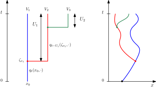
Figure 3: $K$-spine with $K=3$. Left panel: planar tree $\mathbb{T}$ generated from $2$ i.i.d. uniform random variables $(U_{1},U_{2})$. Right panel: branching $1$-spines running along the branches of the tree ${\mathbb{T}}$.

The resulting planar marked ultrametric tree will be referred to as the $K$-spine. We will denote by $Q^{K,t}_{x}$ the distribution of the $K$-spine rooted at $x$. The $t$ superscript refers to the depth of the underlying genealogy. Note that $Q^{K,t}_{x}$ has an implicit dependence on $N$ by our choice of $L$ – see (17). To ease the notation, this dependence will be dropped in the notation.

In the following, $\cal B$ will denote the set of $K-1$ branching points of the $K$-spine; $\cal L$ will denote the set of $K$ leaves. We will denote by $\zeta_{v}$ the mark (or the position) of the spine at a node $v\in\cal B\cup\cal L$. For $v\in{\cal B}$, $|v|$ will denote the time component of the branching point. Finally, $(V_{i};i\in[K])$ is the enumeration of the leaves from left to right in the $K$-spine (i.e., $V_{i}$ is the leaf with label $i$). We will also need the accelerated version of the $K$-spine.

Definition 5 (Accelerated $K$-spine).

Consider the $1$-spine accelerated by $N$, i.e. the transition kernel of the $1$-spine is now given by $q_{tN}(x,y)\equiv q^{L}_{tN}(x,y)$. We denote this kernel by $\bar{q}_{t}(x,y)$. Consider the same planar structure as before, i.e., the depth is $t$ and the distance between points at time $t$ is given by (19). We denote by $\bar{Q}_{x}^{K,t}$ the distribution of the $K$-spine obtained by running accelerated spines along the branches. For any vertex $v$ in the accelerated $K$-spine, $\bar{\zeta}_{v}$ will denote the mark of the vertex $v$.

Proposition 2.7 (Rescaled many-to-few).

Let $t>0$. Let $(\varphi_{i};i\in[K])$ and $(\psi_{i,j};i,j\in[K])$ be measurable bounded functions and define

$$\forall M=[X,d,\nu],\ \ \Psi(M)\ =\ \int\prod_{i,j}1(v_{i}\neq v_{j})\psi_{i,j}(d(v_{i},v_{j}))\prod_{i}\varphi(x_{i})\nu(dv_{i}\otimes dx_{i}).$$

Let $h$ be defined as in (18). Then

$${\mathbb{E}}_{x}\left(\Psi(\bar{M}^{L}_{t})\right)\ =\ \frac{1}{N}K!\ h(0,x)\ t^{K-1}\bar{Q}_{x}^{K,t}\left(\bar{\Delta}\prod_{i,j}\psi_{i,j}(U_{\sigma_{i},\sigma_{j}})\prod_{i}\varphi_{i}(\bar{\zeta}_{V_{\sigma_{i}}})\right),$$

where

$$\bar{\Delta}:=\prod_{v\in{\cal B}}r({\bar{\zeta}_{v}})h(|v|N,\bar{\zeta}_{v})\prod_{v\in{\cal L}}\frac{1}{h(tN,\bar{\zeta}_{v})}.$$

The second crucial result is the following convergence theorem.

Theorem 4.

Let $(\tilde{\varphi}_{i};i\in[K])$ and $(\psi_{i,j};i,j\in[K])$ be continuous bounded functions. Assume further that the $\tilde{\varphi}_{i}$’s are compactly supported in $(0,\infty)$. As $N\to\infty$,

$$\bar{Q}_{x}^{K,t}\left(\bar{\Delta}\prod_{i,j}\psi_{i,j}(U_{\sigma_{i},\sigma_{j}})\prod_{i}\tilde{\varphi}_{i}(\bar{\zeta}_{V_{\sigma_{i}}}){h^{\infty}(\bar{\zeta}_{V_{\sigma_{i}}})}\right)\ \to\left(\frac{\Sigma^{2}}{2}\right)^{K-1}{\mathbb{E}}\left(\prod_{i,j}\psi_{i,j}(U_{\sigma_{i},\sigma_{j}})\right)\prod_{i}\int_{{\mathbb{R}}_{+}}\tilde{\varphi}_{i}(x)\Pi^{\infty}(dx).$$

Let us now give a brief heuristics underlying the previous result. By definition

$$\bar{Q}_{x}^{K,t}\left(\bar{\Delta}\prod_{i,j}\psi_{i,j}(U_{\sigma_{i},\sigma_{j}})\prod_{i}{\tilde{\varphi}_{i}}(\bar{\zeta}_{V_{\sigma_{i}}}){h^{\infty}(\bar{\zeta}_{V_{\sigma_{i}}})}\right)\\ =\ \bar{Q}_{x}^{K,t}\left(\prod_{v\in\cal B}r(\bar{\zeta}_{v}){h(|v|N,\bar{\zeta}_{v})}\prod_{i,j}\psi_{i,j}(U_{\sigma_{i},\sigma_{j}})\prod_{i}\tilde{\varphi}_{i}(\bar{\zeta}_{V_{\sigma_{i}}}){\frac{h^{\infty}(\bar{\zeta}_{V_{\sigma_{i}}})}{h(tN,\bar{\zeta}_{V_{\sigma_{i}}})}}\right).$$

The branching structure for the $K$-spine is binary a.s. whereas the spines running along the branches are accelerated by $N$. We will show later on that under ($H_{fp}$), $h(tN,x)\approx h^{\infty}(x),\tilde{h}(tN,x)\approx\tilde{h}^{\infty}(x)$ for $N$ large. From Proposition 2.6, as $N\to\infty$,

$$\Pi(dx)\approx\Pi^{\infty}(dx)=h^{\infty}(x)\tilde{h}^{\infty}(x)dx\ =\ \frac{v_{1}^{\infty}(x)}{||v_{1}^{\infty}||^{2}}dx.$$

It is now reasonable to believe that, provided enough mixing, the RHS can be approximated by

$$\left(\int_{0}^{\infty}h^{\infty}(x)r(x)\Pi^{\infty}(dx)\right)^{K-1}\mathbb{E}\left(\prod_{i,j}\psi_{i,j}(U_{\sigma_{i},\sigma_{j}})\right)\prod_{i}\int\tilde{\varphi}_{i}(x)\Pi^{\infty}(dx),$$

assuming the values of the spine at the branching points and the leaves converge to a sequence of i.i.d. random variables with law $\Pi^{\infty}$. This yields the content of Theorem 4.

Challenge 1.

The previous argument relies on a $k$-mixing property of the $1$-spine. This analysis will be carried out in Section 4 using Sturm–Liouville theory.

2.5 Limiting moments

Let us now demonstrate the importance of Theorem 4. Let

$$\forall M=[X,d,\nu],\ \ \tilde{\Psi}(M)\ :=\ \int_{X}\prod_{i,j}\psi_{i,j}(d({v_{i},v_{j}}))\prod_{i}\tilde{\varphi}_{i}(x_{i})h^{\infty}(x_{i})\ \nu(dv_{i}\otimes dx_{i}).$$

for any bounded continuous functions $\tilde{\varphi}_{i},\psi_{i,j}$ such that the $\tilde{\varphi}_{i}$ are compactly supported. From the many-to-few formulae, Theorem 4 entails

$${\mathbb{E}}_{x}\left(\tilde{\Psi}(\bar{M}^{L}_{t})\right) = \ \mathbb{E}_{x}\bigg{(}\int\prod_{i,j}\psi_{i,j}(\bar{d}({v_{i},v_{j}}))\prod_{i}\tilde{\varphi}_{i}(x_{i})h^{\infty}(x_{i})\ \bar{\nu}_{t}^{L}(dv_{i}\otimes dx_{i})\bigg{)}$$

$$\approx \ \mathbb{E}_{x}\bigg{(}\int\prod_{i,j}1(v_{i}\neq v_{j})\psi_{i,j}(\bar{d}({v_{i},v_{j}}))\prod_{i}\tilde{\varphi}_{i}(x_{i})h^{\infty}(x_{i})\ \bar{\nu}_{t}^{L}(dv_{i}\otimes dx_{i})\bigg{)}$$

$$\approx \frac{2h^{\infty}(x)}{N\Sigma^{2}t}\ \times\ K!\left(t\frac{\Sigma^{2}}{2}\right)^{K}{\mathbb{E}}\left(\prod_{i,j}\psi_{i,j}(U_{\sigma_{i},\sigma_{j}})\right)\prod_{i}\int_{{\mathbb{R}}_{+}}\tilde{\varphi}_{i}(x)\Pi^{\infty}(dx).$$

Let us formally take $\psi_{i,j}\equiv 1$ and $\tilde{\varphi}_{i}\equiv 1/h^{\infty}$ in the previous expression (note that this is problematic since $\tilde{\varphi}_{i}$ is neither bounded nor compactly supported, see Challenge 4 below). Then for large $N$,

$${\mathbb{E}}_{x}\left(\left(\frac{1}{N}Z_{tN}^{L}\right)^{K}\right)\ \approx\ \ \frac{2h^{\infty}(x)}{N\Sigma^{2}t}\ \ \times\ \ \underbrace{K!\left(t\frac{\Sigma^{2}}{2}\right)^{K}}_{\mbox{exponential moments}}\times\quad{\underbrace{\int_{0}^{\infty}\tilde{h}^{\infty}(x)dx}_{=1}},$$

where we used the fact that $\tilde{h}^{\infty}=\Pi^{\infty}/h^{\infty}$. Now, the RHS coincides with the moments of a r.v. with law

$$\left(1-\frac{2h^{\infty}(x)}{N\Sigma^{2}t}\right)\delta_{0}(dx)+\frac{2h^{\infty}(x)}{N\Sigma^{2}t}\exp\left(-\frac{2x}{\Sigma^{2}t}\right)\frac{2dx}{\Sigma^{2}t}.$$

If we identify the Dirac measure at $0$ with the extinction probability, this suggests the Kolmogorov estimate and the Yaglom law exposed in Theorem 1 and Theorem 2. Further, if we replace $\tilde{\varphi}_{i}=\varphi_{i}/h^{\infty}$ in Theorem 4 (again a problematic step), the previous estimates entail

$${\mathbb{E}}_{x}\left(\Psi(\bar{M}^{L}_{t})\big{|}Z_{tN}^{L}>0\right)\approx K!{\mathbb{E}}\left(\prod_{i,j}\psi_{i,j}(U_{\sigma_{i},\sigma_{j}})\right)\prod_{i}\int_{{\mathbb{R}}_{+}}\varphi_{i}(x)\left(t\frac{\Sigma^{2}}{2}\right){\tilde{h}^{\infty}(x)dx.}$$

where $\Psi(M)$ is now an arbitrary product polynomial of the form

$$\Psi(M)\ :=\ \int\prod_{i,j}\psi_{i,j}({d(v_{i},v_{j})})\prod_{i}\varphi_{i}(x_{i})\nu(dv_{i}\otimes dx_{i}).$$

According to Proposition 2.4, this coincides with the moments of the Brownian CPP described in Theorem 3.

Challenge 2.

The previous computation only suggests that the probability for the population to be $o(\frac{1}{N})$ is given by the Kolmogorov estimate. Intuitively, the Dirac mass above corresponds to a population whose size becomes invisible at the limit after rescaling the population by $N$. It thus remains to show that if the population is small compared to $N$ then it must be extinct. This will be carried out in Section 6.

Challenge 3.

Going from Theorem 4 to the convergence of the $M_{tN}^{L}$ requires to use test functions exploding at the boundary. To overcome this technical difficultly, we will impose an extra thinning of the population by killing all the particles close to the boundaries at time $tN$. This final technical step will be carried in Section 7 using some general property of the Gromov-weak topology.

2.6 Choosing the cutoff $L$

We now motivate our choice for $L$. According to the previous arguments, we want to choose $L$ large enough such that on time scale $O(N)$

• The particles do not reach $L$ with high probability. This will imply that $\bar{M}_{t}^{L}$ and $\bar{M}_{t}$ coincide with high probability.

• The $1$-spine reaches equilibrium in a time $o(N)$ regardless of its initial position on $[0,L]$. This is needed to justify the calculations of Section 2.4.

(i) Hitting the right boundary. Let $E$ be a compact set in the vicinity of the boundary $L$ (say $[L-2,L-1]$). Recall from the discussion after Proposition 1.3 that for $x\geq 1$,

$$h^{\infty}(x)=\frac{1}{\tilde{c}\|v_{1}\|^{2}}\,e^{\mu x}v_{1}^{\infty}(x)\approx\frac{1}{\tilde{c}\|v_{1}^{\infty}\|^{2}}\,e^{\beta}e^{(\mu-\beta)x}.$$

A direct application of the many-to-few lemma with $K=1$ (many-to-one) and $\varphi_{1}(x)=\mathbb{1}_{x\in E}$ implies that

$$\mathbb{E}_{x}\left[\sum_{v\in\mathcal{N}^{L}_{tN}}\mathbb{1}_{x_{v}\in E}\right] = \int_{E}\frac{h(0,x)}{h(tN,y)}q_{tN}(x,y)dy\approx\int_{E}\frac{h^{\infty}(x)}{h^{\infty}(y)}\Pi^{\infty}(dy)\approx h^{\infty}(x)O(\overbrace{e^{-\frac{\mu+\beta}{\mu-\beta}\log(N)}}^{=N^{-\alpha}}),$$

where the last approximation holds under the assumption that $E$ is a compact set close to $L$. Integrating on $[0,tN]$, this yields that the occupation time of the set $E$ on the time interval $[0,tN]$ is $O(N^{1-\alpha})$. Recall that the probability of survival is of order $1/N$ so that the occupation time of the conditioned process is $O(N^{2-\alpha})$. Recalling that $\alpha>2$ under ($H_{fp}$), this yields the desired estimate.

(ii) Mixing time. Recall from the discussion after Proposition 1.3 that $v_{1}(x)\approx e^{-\beta(x-1)}$ for $x\geq 1$ and $L$ large enough. As a consequence, the $1$-spine (see Definition 4) is well approximated by the diffusion

$$dz_{t}=-\beta dt+dw_{t}\ \ \mbox{for $z_{t}\geq 1$}.$$

A good proxy for the mixing time is the first returning time at $1$ which is of the order $\log(N)=o(N)$ for every $x\in[1,L]$, as desired. A more refined analysis will be carried in Section 4.

3 The many-to-few theorem

3.1 The general case

In this section, we consider a general BBM killed at the boundary of a regular open domain $\Omega\subset\mathbb{R}^{d}$. Unless otherwise specified, we used the same notation as in the previous sections. We will assume that

1. The generator of a single particle is given by a differential operator

   $${\cal L}f(x)\ =\ \frac{1}{2}\sum_{i,j}a_{ij}(x)\partial_{x_{i}x_{j}}f(x)\ +\ \sum_{i}b_{i}(x)\partial_{x_{i}}f(x),\quad x\in\Omega,$$ (20)

   $$f(x) =0,\quad x\in\partial\Omega.$$

   We assume that $(a_{ij})$ is uniformly elliptic, which means that there exists a constant $\theta>0$ such that for all $\xi\in\mathbb{R}^{d}$ and a.e. $x\in\Omega$, $\sum_{i,j=1}^{d}a_{ij}(x)\xi_{i},\xi_{j}\geq\theta\|\xi\|^{2}$ (see [Eva10, §6.1]). In addition, we assume that $a_{i,j}\in\mathcal{C}^{1}(\Omega)$ and $\sup_{x\in\Omega}|b_{i}(x)|<\infty$ for all $1\leq i,j\leq d$.

2. A particle at location $x$ branches into two particles at rate $r(x)$ (we only consider binary branching).

We denote by ${\cal N}_{t}$ the set of particles alive at time $t$. For any pair of particles $v,w\in{\cal N}_{t}$, $d(u,w)$ will denote the time to their most recent common ancestor. Finally, we define the random mmm space

$$M_{t}\ =\ [{\cal N}_{t},d,\nu_{t}],\ \ \mbox{where $\nu_{t}=\sum_{v\in{\cal N}_{t}}\delta_{v,x_{v}}$}.$$

We say that a function $h(x)$ is harmonic if and only $h$ satisfies the Dirichlet problem

$$\begin{array}[]{c}{\cal B}h(x):={\cal L}h(x)+r(x)h(x)=0,\ \ \mbox{for every $x\in\Omega$,}\\ h(x)=0,\ \ \mbox{for $x\in\partial\Omega$}.\end{array}$$

Definition 6.

The $1$-spine whose generator is given by the Doob $h$-transform of the differential operator ${\cal B}$

$$\frac{{\cal B}(hf)}{h}(x) =\frac{1}{2}\sum_{i,j}a_{ij}(x)\left(\partial_{x_{i}x_{j}}f(x)+\frac{\partial_{x_{i}}h}{h}\partial_{x_{j}}f(x)+\frac{\partial_{x_{j}}h}{h}\partial_{x_{i}}f(x)\right)+\sum_{i}b_{i}(x)\partial_{x_{i}}f(x),\quad x\in\Omega,$$

$$f(x) =0,\quad x\in\partial\Omega,$$

where the first equality is a direct consequence of the fact that $h$ is harmonic. We will denote by $q_{t}(x,y)$ the transition probability at time $t$. The $K$-spine distribution $Q^{K,t}_{x}$ is defined analogously to Section 2.4.

Our many-to-few formulae rely on a uniform planarisation of the BBM that we now describe. At every time $t>0$, every particle is now endowed with two marks $({x_{v}},p_{v})$ where $p_{v}\in\cup_{n\in\mathbb{N}}\{0,1\}^{n}$. As before, ${x_{v}}$ denotes the position of the particle. The planarisation marks $p_{v}$ are assigned recursively as follows. We mark the root with $\emptyset$ and

1. At every branching point $v$, we distribute the marks $(p_{v},0)$ and $(p_{v},1)$ uniformly among the two children: $(p_{v},0)$ (resp. $(p_{v},1)$) is said to the left (resp. right) child of $v$.

2. The mark $p_{v}$ does not vary between two branching points, i.e., $p_{v_{1}}=p_{v_{2}}$ if the trajectory connecting $v_{1}$ and $v_{2}$ does not encounter any branching points.

Let ${\cal N}_{t}^{pl}$ be the the set particles at time $t$ in the planar BBM. For every $K$-uplet $v_{1},v_{2}\cdots,v_{K}$ in ${\cal N}_{t}^{pl}$, let

$${\mathbb{U}}(\vec{v})\ =\ [X(\vec{v}),d(\vec{v}),\nu(\vec{v})]$$

be the planar mmm space induced by this set of vertices. The space consists of the set of vertices ancestral to the vertices in $\vec{v}$. In particular, ${\mathbb{U}}(\vec{v})$ is binary and made of $K$ leaves and $K-1$ branching points. The measure is given by the counting measure on the leaves

$$\nu(\vec{v})=\sum_{\vec{v}}\delta_{v,({x_{v}},p_{v})}$$

so that the support of $\nu$ is given by the set of leaves $\vec{v}$ and the cardinality of the support is $K$.

Let us now introduce some definition. If $\mathbb{U}(\vec{v})=U$, the set of branching points of $U$ will be denoted by ${\cal B}\equiv{\cal B}(U)$ and $\vec{v}={\cal L}\equiv{\cal L}(U)$ will refer to the set of leaves. We define $T_{0}(U)$ (resp. $T_{1}(U)$) to be the left (resp. right) subtree attached to the MRCA (Most Recent Common Ancestor) of the sample and we denote by $x_{MRCA}(U)$ the spatial position of the MRCA. Finally, let $\tau(U)=\max_{u\neq w}d(u,w)$ (where the maximum is taken over the pair of distinct leaves in $U$).

Lemma 3.1 (Many-to-one).

For every bounded continuous function $f$

$$\mathbb{E}_{x}\left[\sum_{v\in{\cal N}_{t}}f({x}_{v})\right]\ =\ \int_{\Omega}f(y)q_{t}(x,y)\frac{h(x)}{h(y)}dy.$$

Proof.

One can readily check that $p_{t}(x,y):=q_{t}(x,y)\frac{h(x)}{h(y)}$ are the fundamental solutions of the same PDE

$$\begin{cases}\partial_{t}u(t,y)=\mathcal{L}^{*}u(t,y),&y\in\Omega,\\ u(t,y)=0,&y\in\partial\Omega,\end{cases}$$

where $\mathcal{L}^{*}$ is the adjoint of the differential operator (20). ∎

Lemma 3.2.

Let $K\in\mathbb{N}$ and $t>0$. Define the measure $R^{K,t}_{x}$ on the set of planar mmm so that for every bounded measurable function $F$,

$$R^{K,t}_{x}(F)\ :=\ \mathbb{E}_{x}\left(\sum_{v_{1}<\cdots<v_{K},\ v_{i}\in{\cal N}_{t}^{pl}}F({\mathbb{U}}(\vec{v}))\right).$$

Then

$$R^{K,t}_{x}(F)\ =\ \ h(x)t^{K-1}\ Q_{x}^{K,t}(\Delta F)\ \ \mbox{with $\Delta=\prod_{v\in{\cal B}}r(\zeta_{v})h(\zeta_{v})\prod_{v\in{\cal L}}\frac{1}{h(\zeta_{v})}$}.$$

Proof.

We will show the result by an induction of $K$. The case $K=1$ is the many-to-one lemma. Let us now consider $F$ of the following product form

$$F(U)\ =\ f(\tau(U))\psi_{0}(T_{0}(U))\psi_{1}(T_{1}(U)).$$

Then

$$R^{K,t}_{x}(F) = \mathbb{E}_{x}\left(f(\tau(U))\sum_{n=1}^{K-1}\left(\sum_{v_{1}<\cdots<v_{n},v_{i}\in T_{0}(U),|v_{i}|=t}\psi_{0}(\mathbb{U}(\vec{v}))\right)\left(\sum_{w_{1}<\cdots<w_{K-n},w_{i}\in T_{1}(U),|w_{i}|=t}\psi_{1}(\mathbb{U}(\vec{w}))\right)\right),$$

where the ordering in the sum is meant in the planar sense and $|v|=t$ means that $v\in{\cal N}_{t}^{pl}$. By the Markov property, we have

$$R^{K,t}_{x}(F) = \mathbb{E}_{x}\left(\sum_{v_{1}<\cdots<v_{K},\ |v_{i}|=t}F({\mathbb{U}}(\vec{v}))\right)$$

$$= \mathbb{E}_{x}\left(\int_{0}^{t}f(s)\sum_{v\in{\cal N}_{t-s}^{pl}}{r({x_{v}})}\sum_{n=1}^{K-1}\mathbb{E}_{{x_{v}}}\left(\sum_{v_{1}<\cdots<v_{n},|v_{i}|=s}\psi_{0}(\mathbb{U}(\vec{v}))\right)\mathbb{E}_{{x_{v}}}\left(\sum_{w_{1}<\cdots<w_{K-n},|w_{i}|=s}\psi_{1}(\mathbb{U}(\vec{w}))\right)ds\right).$$

By the many-to-one formula, the RHS is equal to

$$h(x)\int_{0}^{t}f(s)\int_{y\in\Omega}r(y)\frac{q_{t-s}(x,y)}{h(y)}\sum_{n=1}^{K-1}\mathbb{E}_{y}\left(\sum_{v_{1}<\cdots<v_{n},|v_{i}|=s}\psi_{0}(\mathbb{U}(\vec{v}))\right)\mathbb{E}_{y}\left(\sum_{w_{1}<\cdots<w_{K-n},|w_{i}|=s}\psi_{1}(\mathbb{U}(\vec{w}))\right)dyds.$$

By induction

$$\mathbb{E}_{y}\left(\sum_{v_{1}<\cdots<v_{n},|v_{i}|=s}\psi_{0}(\mathbb{U}(\vec{v}))\right) = h(y)s^{n-1}Q^{n,s}_{y}(\Delta\psi_{0}),$$

$$\mathbb{E}_{y}\left(\sum_{w_{1}<\cdots<w_{K-n},|w_{i}|=s}\psi_{1}(\mathbb{U}(\vec{w}))\right) = h(y)s^{K-n-1}Q^{K-n,s}_{y}(\Delta\psi_{1}).$$

As a consequence,

$$R^{K,t}_{x}(F) = h(x)\int_{0}^{t}f(s)s^{K-2}\int_{y\in\Omega}r(y)\frac{q_{t-s}(x,y)h(y)^{2}}{h(y)}\sum_{n=1}^{K-1}Q_{y}^{n,s}(\Delta\psi_{0})Q_{y}^{K-n,s}(\Delta\psi_{1})dyds$$

$$= h(x)t^{K-1}\int_{0}^{t}f(s)\frac{(K-1)s^{K-2}}{t^{K-1}}\int_{y\in\Omega}r(y)q_{t-s}(x,y)h(y)\sum_{n=1}^{K-1}\frac{1}{K-1}Q_{y}^{n,s}(\Delta\psi_{0})Q_{y}^{K-n,s}(\Delta\psi_{1})dyds.$$

It remains to show that

$$Q^{K,t}_{x}(F)=\int_{0}^{t}f(s)\underbrace{\frac{(K-1)s^{K-2}}{t^{K-1}}}_{(i)}\int_{y\in\Omega}q_{t-s}(x,y)\underbrace{r(y)h(y)}_{(v)}\sum_{n=1}^{K-1}\underbrace{\frac{1}{K-1}}_{(ii)}\underbrace{Q_{y}^{n,s}(\Delta\psi_{0})Q_{y}^{K-n,s}(\Delta\psi_{1})}_{(iii)}dyds.$$ (21)

This follows from the next observations

1. The depth $\tau(U)$ of the deepest branch is distributed as $\max(U_{1},\cdots,U_{K-1})$, where the $U_{i}$’s are i.i.d. random variables uniform on $[0,t]$. The density of this variable is given by (i).

2. The index $I$ of the deepest branch is chosen uniformly at random in $[K-1]$.

3. Let us condition on $I=n$, the position $x_{MRCA}(U)=y$ and $\tau(U)=s$. Then the left and right subtrees $T_{0}$ and $T_{1}$ are independent and are distributed as $n$ and $K-n$ spines with depth $s$ respectively. By the Markov property, the initial condition of each spine is a single particle at $y$.

4. $x_{MRCA}(U)$ is distributed as the $1$-spine at time $t-s$.

5. If $x_{MRCA}(U)=y,\tau(U)=s$, then

   $$\Delta(U)={r(y)}h(y)\Delta(T_{0}(U))\Delta(T_{1}(U))$$

∎

Theorem 5 (Many-to-few).

Let $t>0$. Let $(\varphi_{i};i\in[K])$ and $(\psi_{i,j};i,j\in[K])$ be continuous bounded functions. Define the product polynomial

$$M=[X,d,\nu],\ \ \Psi(M)\ :=\ \int\prod_{i,j}\mathbb{1}_{v_{i}\neq v_{j}}\psi_{i,j}(d({v_{i},v_{j}}))\prod_{i}\varphi_{i}(x_{i})\nu(dv_{i}\otimes dx_{i}).$$

Then

$$\mathbb{E}_{x}\left(\Psi(M_{t})\right)\ =K!\ h(x)\ t^{K-1}Q_{x}^{K,t}\left(\Delta\prod_{i,j}\psi_{i,j}(U_{\sigma_{i},\sigma_{j}})\prod_{i}\varphi_{i}(\zeta_{V_{\sigma_{i}}})\right),$$

where $\sigma$ is an independent random permutation of $[K]$.

Proof.

$[X,d,\nu]$ be a random mmm such that the support of $\nu$ is a set of cardinality $K$ a.s.. In our case, the support is given by the set of $K$ leaves of the sample. Define

$$F(U)\ =\ \frac{1}{K!}\sum_{\sigma\in S_{K}}\prod_{i,j}\psi_{i,j}(d(V_{\sigma_{i}},V_{\sigma_{j}}))\prod_{i}\varphi_{i}(x_{V_{\sigma_{i}}}),$$

where $(V_{1},\cdots,V_{K})$ is an arbitrary labelling of the support of $\nu$ and $S_{K}$ is the set of permutations of $[K]$. Note that this functional does not depend on the labelling so that $F$ is constant on a given isometric class.

We have

$$\mathbb{E}_{x}\left(\sum_{v_{1}\neq\cdots\neq v_{K}\in{\cal N}_{t}}\prod_{i,j}\psi_{i,j}(d(v_{i},v_{j}))\prod_{i}\varphi_{i}(x_{v_{i}})\right) = \mathbb{E}_{x}\left(K!\sum_{v_{1}<\cdots<v_{K}\in{\cal N}_{t}}\frac{1}{K!}\sum_{\sigma\in S_{K}}\prod_{i,j}\psi_{i,j}(d(v_{\sigma_{i}},v_{\sigma_{j}}))\prod_{i}\varphi_{i}(x_{v_{\sigma_{i}}})\right)$$

$$= K!\mathbb{E}_{x}\left(\sum_{v_{1}<\cdots<v_{K}\in{\cal N}_{t}}F({\mathbb{U}}(\vec{v}))\right).$$

The result immediately follows from Lemma 3.2. ∎

3.2 The subcritical BBM

We now apply the previous setting to the problem at hands. The idea is to enrich the mark space by adding time as an extra variable. More precisely, for every $v\in{\cal N}_{t}^{L}$, we equip $v$ with a two dimensional mark $(t,x_{v})$ where $x_{v}$ is the position of the particle on $[0,L]$.

Lemma 3.3.

Let $\mu,\lambda_{1},\lambda_{1}^{\infty},r(x)$ be defined as in Section 1. Define

$${\cal L}f(t,x)\ =\partial_{t}f(t,x)+\frac{1}{2}\partial_{xx}f(t,x)-\mu\partial_{x}f(t,x),\ \ \mbox{$f(t,0)=f(t,L)=0$.}$$

Then, the function $h$ defined in (18) is harmonic. In addition,

$$\frac{{\cal B}(hf)}{h}(t,x)\ =\ \partial_{t}f(t,x)+\ \frac{1}{2}\partial_{xx}f(t,x)+\frac{v_{1}^{\prime}(x)}{v_{1}(x)}\partial_{x}f(t,x).$$

Proof.

This is a straightforward consequence of Definition 6. ∎

A direct application of Theorem 5 entails the following result.

Corollary 3.4 (Many-to-few).

Let $t>0$. Let $(\varphi_{i};i\in[K])$ and $(\psi_{i,j};i,j\in[K])$ be measurable bounded functions. Define the product polynomial

$$M=[X,d,\nu],\ \ \Psi(M)\ :=\ \int\prod_{i,j}\mathbb{1}_{v_{i}\neq v_{j}}\psi_{i,j}(d({v_{i},v_{j}}))\prod_{i}\varphi_{i}(x_{i})\nu(dv_{i}\otimes dx_{i}).$$

Then

$$\mathbb{E}_{x}\left(\Psi{(M^{L}_{t})}\right)\ =\ K!\ {h(0,x)}\ t^{K-1}Q_{x}^{K,t}\left(\Delta\prod_{i,j}\psi_{i,j}(U_{\sigma_{i},\sigma_{j}})\prod_{V_{i}\in{\cal L}}\varphi_{i}(\zeta_{V_{\sigma_{i}}})\right),$$

where $\sigma$ is an independent permutation of $[K]$ and

$$\Delta:=\prod_{v\in{\cal B}}r({\zeta_{v}})h(|v|,\zeta_{v})\prod_{v\in{\cal L}}\frac{1}{h(t,{\zeta_{v}})}.$$

Proof of Proposition 2.7.

This is a direct consequence Corollary 3.4 after rescaling the measure by $N$ and time by $N$. ∎

4 Spectral theory

In this section, we examine the density of the particles in $\mathbf{X}^{L}$. In Section 4.1 and Section 4.2, we give precise estimates on the heat kernel $p_{t}$ associated to (A) and compute the relaxation time of the system. All the lemmas in these sections hold under ($H_{p}$) and do not require the additional assumption ($H_{fp}$). Sections 4.3 and 4.4 are aimed at quantifying the fluctuations in $\mathbf{X}^{L}$ and are specific to the fully pushed regime.

4.1 Preliminaries

Consider the Sturm–Liouville problem (SLP) together with boundary conditions (BC). Let us first recall some well-known facts about Sturm–Liouville theory following [Zet12, Section 4.6]:

• A solution of (SLP) is defined as a function $v:[0,L]\to\mathbb{R}$ such that $v$ and $v^{\prime}$ are absolutely continuous on $[0,L]$ and satisfies (SLP) a.e. on $(0,L)$. In particular, any solution $v$ is continuously differentiable on $[0,L]$. Since $f$ is continuous on $[0,L]$, the solutions are also twice differentiable on $[0,L]$ and (SLP) holds for all $x\in(0,L)$.

• A complex number $\lambda$ is an eigenvalue of the Sturm–Liouville problem (SLP) with boundary conditions (BC) if Equation (SLP) has a solution $v$ which is not identically zero on $[0,L]$ and that satisfies (BC). This set of eigenvalues will be referred to as the spectrum.

• It is known that this set of eigenvalues is infinite, countable and it has no finite accumulation point. Besides, it is upper bounded and all the eigenvalues are simple and real so that they can be numbered

  $$\lambda_{1}>\lambda_{2}>...>\lambda_{n}>...$$

  where

  $$\lambda_{n}\rightarrow-\infty\quad\textnormal{ as }\quad n\rightarrow+\infty.$$

  We will denote by $K$ the largest integer such that

  $$\lambda_{K}>0.$$

• As a consequence, the eigenvector $v_{i}$ associated to $\lambda_{i}$ is unique up to constant multiplies. Furthermore, the sequence of eigenfunctions can be normalised to be an orthonormal sequence of $\mathrm{L}^{2}([0,L])$. This orthonormal sequence is complete in $\mathrm{L}^{2}([0,L])$ so that the fundamental solution of PDE (B) can be written as

  $$g_{t}(x,y)=\sum_{k=1}^{\infty}e^{\lambda_{k}t}\frac{v_{k}(x)v_{k}(y)}{\|v_{k}\|^{2}}.$$ (22)

• The function $v_{1}$ does not change sign in $(0,L)$. More generally, the eigenfunction $v_{k}$ has exactly $k-1$ zeros on $(0,L)$.

• The eigenvalues and the eigenvectors of (SLP) with boundary conditions (BC) can be characterised through the Prüfer transformation (see [Zet12, Section 4.5]). For all $\lambda\in\mathbb{R}$, consider the Cauchy problems

  $$\dot{\theta}_{\lambda}(x)=\cos^{2}(\theta_{\lambda}(x))+(W(x)-2\lambda)\sin^{2}(\theta_{\lambda}(x)),\quad\theta_{\lambda}(0)=0,$$ (23)

  and

  $$\dot{\rho}_{\lambda}(x)=\left(\frac{1-W(x)}{2}+\lambda\right)\sin(2\theta_{\lambda}(x))\rho_{\lambda}(x),\quad\rho_{\lambda}(0)=1.$$ (24)

  Note that (23) and (24) have a unique solution defined on $[0,+\infty)$ for each $\lambda\in\mathbb{R}$. The eigenvalue $\lambda_{k}$ is characterised as the unique solution of $\theta_{\lambda}(L)=k\pi$.

  Note that for all $\lambda^{*}<\lambda$,

  $$0\leq\theta_{\lambda}(x)\leq\theta_{\lambda*}(x),\quad\forall x\in[0,L].$$ (25)

  If $u_{k}$ is the eigenvector associated to $\lambda_{k}$ such that $u_{k}^{\prime}(0)=1$, then

  $$u_{k}(x)=\rho_{\lambda_{k}}(x)\sin(\theta_{\lambda_{k}}(x)),\quad u_{k}^{\prime}(x)=\rho_{\lambda_{k}}(x)\cos(\theta_{\lambda_{k}}(x)),\quad\forall x\in[0,L].$$ (26)

• Denote by $\bar{\lambda}_{1}>\bar{\lambda}_{2}>...$ the eigenvalues of the Sturm–Liouville problem

  $$\frac{1}{2}v^{\prime\prime}(x)+\frac{1}{2}\|W\|_{\infty}\mathbb{1}_{[0,1]}(x)v(x)=\lambda v(x),\quad v(0)=v(L)=0.$$

  and by $\underline{\lambda}_{1}>\underline{\lambda}_{2}>...$ the eigenvalues of the Laplacian with homogeneous Dirichlet boundary conditions (at $0$ and $L$). Then, for all $k\in\mathbb{N}$,

  $$\underline{\lambda}_{k}\leqslant\lambda_{k}\leqslant\bar{\lambda}_{k}.$$ (27)

  See [Zet12, Theorem 4.9.1] for a proof of this comparison principle. Recall that

  $$\underline{\lambda}_{k}=-\frac{k^{2}\pi^{2}}{2L^{2}},$$ (28)

  and that the eigenvalues $(\bar{\lambda}_{k})$ have been fully characterised in [Tou21]. See (10) for a characterisation of the negative spectrum for a special case of $W$. In particular, we know that there exists $\bar{K}\geq K$ that is fixed for $L$ large enough and such that $\bar{\lambda}_{k}>0$ for all $k\geq\bar{K}$ and $\bar{\lambda}_{k}<0$ for all $k<\bar{K}$.

• For fixed $i\in\mathbb{N}$, the eigenfunction $\lambda_{i}$ is an increasing function of $L$ (see e.g. [Zet12, Theorem 4.4.4]). Since $\lambda_{1}$ converges, the $i$-th eigenvalue $\lambda_{i}$ also converges. Furthermore, by (27), this implies that the number of positive eigenvalues $K$ is fixed for $L$ large enough. For $i>K$, this limit, that we denote by $\lambda_{i}^{\infty}$ is positive and we have

  $$\lambda_{1}^{\infty}\geq\lambda_{2}^{\infty}\geq\lambda_{3}^{\infty}\geq...\geq\lambda_{K}^{\infty}.$$

  We will prove below that these inequalities are strict inequalities.

Throughout the article, the eigenvector $v_{1}$ will be chosen such that $v_{1}(1)=1$ and $u_{1}$ in such a way that $u_{1}^{\prime}(0)=1$. Note that for $x\in[1,L]$, we have

$$v_{1}(x)=\sinh\left(\sqrt{2\lambda_{1}}(L-x)\right)/\sinh\left(\sqrt{2\lambda_{1}}(L-1)\right).$$ (29)

On $[0,1]$, the eigenvector $u_{1}$ is the unique solution of the Cauchy problem

$$u^{\prime\prime}(x)=\left(2\lambda_{1}-W(x)\right)u(x),\quad u(0)=0,\;u^{\prime}(0)=1.$$ (30)

Lemma 4.1 ([Zet12], Theorem 4.5.1).

Let $a,b,c\in\mathcal{C}([0,1])$. Let $\theta$ and $\rho$ be the solutions of the Cauchy problems

$$\begin{cases}\dot{\theta}(x)=a(x)\cos(\theta(x))^{2}+b(x)\sin(\theta(x))^{2},\quad\theta(0)=0,\\ \dot{\rho}(x)=c(x)\sin(2\theta(x))\rho(x),\quad\rho(0)=1.\end{cases}$$

Let $\Phi$ be the application from $(C([0,1])^{3},||\cdot||_{\infty})$ to $(C(0,1)^{2},||\cdot||_{\infty})$ which maps $(a,b,c)$ to the solutions $(\rho,\theta)$ of the Cauchy problems. Then $\Phi$ is continuous.

The next result is a generalisation of Proposition 1.3 in the introduction.

Lemma 4.2.

Assume that ($H_{p}$) holds. Then,

$$\lambda_{1}^{\infty}-\lambda_{1}=O\left(e^{-2\beta L}\right)=O\left(\frac{1}{N^{\alpha-1}}\right).$$ (31)

As a consequence, for all $0<t\lesssim N$,

$$h(t,x)=\left(1+O\left(e^{(\mu-3\beta)L}\right)\right)h(0,x),\quad x\in[0,L].$$ (32)

In addition,

$$v_{1}(x)\asymp(1\wedge x\wedge(L-x))e^{-\beta x},\quad x\in[1,L],$$ (33)

and we have $v_{1}\mathbb{1}_{\in[0,L]}\to v_{1}^{\infty}$ as $L\to\infty$ pointwise, in $\mathrm{L}^{2}(\mathbb{R}^{+})$ and in ${\cal C}^{1}([0,1])$. Further, $v_{1}^{\infty}(x)=e^{-\beta(x-1)}$ for $x\geq 1$.

Proof.

We first prove the convergence of $u_{1}$. Recall from (26) that $u_{1}(x)=\rho_{\lambda_{1}}(x)\sin(\theta_{\lambda_{1}}(x))$ and $u^{\prime}_{1}(x)=\rho_{\lambda_{1}}(x)\cos(\theta_{\lambda_{1}}(x))$ for all $x\in[0,L]$. By Lemma 4.1, $u_{1}$ converges to $u_{1}^{\infty}=\rho_{\lambda_{1}^{\infty}}\sin(\theta_{\lambda_{1}^{\infty}})$ in $\mathcal{C}^{1}([0,1])$ as $L\to\infty$. The pointwise convergence on $[0,\infty]$ follows from the fact that

$$u_{1}(x)=u_{1}(1)\frac{\sinh(\sqrt{2\lambda_{1}}(L-x))}{\sinh(\sqrt{2\lambda_{1}}(L-1))},\quad\forall x\in[1,L].$$ (34)

The convergence in $\mathrm{L}^{2}$ follows from the uniform convergence on $[0,1]$ and the explicit form of $u_{1}$ on $[1,L]$.

It follows from the integrated version of (30) that $u_{1}^{\prime\prime}$ converges to $(u_{1}^{\infty})^{\prime\prime}$ in $\mathcal{C}([0,1])$ and that $u_{1}^{\infty}$ is the unique solution of the Cauchy problem

$$\frac{1}{2}u^{\prime\prime}(x)+\frac{1}{2}u(x)=\lambda_{1}^{\infty}u(x),\quad x\in(0,1),\quad u_{1}(0)=0,\;u_{1}^{\prime}(0)=1.$$ (35)

As a consequence, $u_{1}^{\infty}(x)\neq 0$ for every $x\in[0,1]$. Indeed, $u_{1}^{\infty}\geq 0$ so that if $u_{1}^{\infty}(x)=0$ then $(u_{1}^{\infty})^{\prime}(x)=0$ and $u_{1}^{\infty}\equiv 0$ on $[0,L]$, which contradicts the fact that $(u_{1}^{\infty})^{\prime}(0)=1$. It easily follows that $u_{1}^{\infty}(x)\asymp x$ on $[0,1]$.

The convergence of $v_{1}$ then follows from the relation $v_{1}(x)=u_{1}(x)/u_{1}(1)$ and the convergence of $u_{1}$. Finally, Equation (33) then follows from (34).

Let us now prove the first part of the lemma. According to [Zet12, Theorem 4.4.4], $L\mapsto\lambda_{1}(L)$ is differentiable on $(1,+\infty)$ and we have

$$\lambda_{1}^{\prime}(L)=\frac{|u_{1}^{\prime}(L)|^{2}}{\|u_{1}\|^{2}}.$$

Yet,

$$u_{1}^{\prime}(L)=u_{1}(1)v^{\prime}_{1}(L)=-u_{1}(1)\sqrt{2\lambda_{1}}\left(\sinh{\sqrt{2\lambda_{1}}(L-1)}\right)^{-1}=O(e^{-\sqrt{2\lambda_{1}}L}).$$

Thus,

$$\lambda_{1}^{\prime}(L)=O(e^{-2\sqrt{2\lambda_{1}}L}).$$

Define $\tilde{L}$ such that $\lambda_{1}>\frac{\lambda_{1}^{\infty}}{2}$ for all $L>\tilde{L}$. Hence, for $L>\tilde{L}$

$$\lambda_{1}^{\infty}-\lambda_{1}\leqslant C\int_{L}^{\infty}e^{-2\sqrt{\lambda_{1}^{\infty}}L^{\prime}}dL^{\prime}\leqslant Ce^{-2\sqrt{\lambda_{1}^{\infty}}L}.$$

This implies that $\lambda_{1}^{\infty}-\lambda_{1}\ll\frac{1}{L}$ so that

$$\sinh(\sqrt{2\lambda_{1}}(L-1))\sim\frac{1}{2}e^{\beta(L-1)},\quad L\to\infty,$$

and

$$\lambda_{1}^{\prime}(L)=\frac{2\lambda_{1}}{\|u_{1}\|^{2}}u_{1}(1)\sinh(\sqrt{2\lambda_{1}}(L-1))^{-2}=O\left(e^{-2\beta L}\right),\quad L\to\infty.$$

Therefore, for $L$ large enough, we obtain

$$\lambda_{1}^{\infty}-\lambda_{1}\leqslant\frac{C}{2}\int_{L}^{\infty}e^{-2\beta L^{\prime}}dL^{\prime}=O(e^{-2\beta L}).$$

This concludes the proof of the (31) and (32).

∎

Corollary 4.3.

Assume that ($H_{p}$) holds. Let $k\in\mathbb{N}$. Let $g:[0,\infty)^{k}\to\mathbb{R}$ and $f:[0,\infty)^{2k}\to\mathbb{R}$ be bounded and continuous test functions. Let $t>0$. We have

$$\int g(x_{1},...,x_{k})\prod_{i=1}^{k}\Pi(dx_{i})\to\int g(x_{1},...,x_{k})\prod_{i=1}^{k}\Pi^{\infty}(dx_{i}),\quad\text{as}\quad L\to\infty,$$

and uniformly in $(t_{1},...,t_{k})\in[0,T]^{k}$, as $N$ goes to $\infty$, we have

$$\int f(x_{1},...,x_{k},h(t_{1}N,x_{1}),...,h(t_{k}N,x_{k}))\prod_{i=1}^{k}\Pi(dx_{i})\to\int f(x_{1},...,x_{k},h^{\infty}(x_{1}),...,h^{\infty}(x_{k}))\prod_{i=1}^{k}\Pi^{\infty}(dx_{i}).$$

Proof.

We restrict ourself to the case $k=1$. The case $k>1$ can be proved along the same lines. We start with the first limit. Since $||v_{1}||\to||v_{1}^{\infty}||$, we need to prove that

$$\int g(x_{1},...,x_{k})\prod_{i=1}^{k}v_{1}^{2}(x_{i})dx_{i}\to\int g(x_{1},...,x_{k})\prod_{i=1}^{k}(v_{1}^{\infty})^{2}(x_{i})dx_{i},\quad\text{as}\quad L\to\infty,$$

We first note that

$$v_{1}(x)\leq v_{1}^{\infty}(x)\quad\forall x\in[1,L].$$

The result then follows from the dominated convergence theorem and the fact that that $v_{1}$ converges to $v_{1}^{\infty}$ uniformly on $[0,1]$. The second limit follows from (32) combined with similar arguments. ∎

Lemma 4.4.

Assume that ($H_{p}$) holds. For all $k\in\mathbb{N}$, we have

$$|u_{k}(x)|\leqslant e^{3\bar{c}}e^{|\lambda_{k}|}(1+2|\lambda_{k}|)x,\quad x\in[0,1],$$

with $\bar{c}=1+\|f\|_{\infty}$.

Proof.

First, note that for all $\lambda\in\mathbb{R}$, the solution $\rho_{\lambda}$ of the Cauchy problem (24) can be expressed as

$$\rho_{\lambda}(x)=\rho_{\lambda}(0)\exp\left(\int_{y=0}^{x}\left(\frac{1-f(y)}{2}+\lambda\right)\sin(2\theta_{\lambda}(y))dy\right),\quad\quad x\in[0,1].$$

Therefore,

$$0\leqslant\rho_{\lambda}(x)\leqslant\exp(\bar{c}+|\lambda|),\quad x\in[0,1].$$ (36)

On the other hand, note that for all $\lambda\in\mathbb{R}$, the unique solution $\theta_{\lambda}$ of (23) is such that

$$\dot{\theta}_{\lambda}(x)-\dot{\theta}_{0}(x)\leqslant|\dot{\theta}_{\lambda}(x)-\dot{\theta}_{0}(x)|\leqslant 2\bar{c}|\theta_{\lambda}(x)-\theta_{0}(x)|+2|\lambda|,\quad x\in[0,1],$$

where we use that $\cos^{2}$ and $\sin^{2}$ are $2$-Lipschitz. Moreover, recall from (25) that $\theta_{\lambda}\geq\theta_{0}$ on $[0,L]$. Hence, for all $\lambda<0$, we have

$$\theta_{\lambda}(x)-\theta_{0}(x)\leqslant-2\lambda x+\int_{y=0}^{x}2\bar{c}(\theta_{\lambda}(y)-\theta_{0}(y))dy,\quad x\in[0,1],$$

and Grönwall’s lemma yields

$$\theta_{\lambda}(x)\leqslant\theta_{0}(x)-2\lambda x\exp(2\bar{c}x),\quad x\in[0,1].$$ (37)

In addition, we see from (23) that $0\leq\theta_{0}(x)\leq\bar{c}x$ for all $x\in[0,L]$, so that

$$\theta_{\lambda}(x)\leqslant(\bar{c}+2|\lambda|e^{2\bar{c}})x,\quad x\in[0,1],$$ (38)

for all $\lambda<0$. For $\lambda>0$, we use that $0\leq\theta_{\lambda}(x)\leq\theta_{0}(x)$ for all $x\in[0,L]$ (see (25)) so that the last inequality still holds for positive $\lambda$. We finally get the result by combining (26), (36), (38) and the facts that $|\sin(x)|\leqslant x$ for all $x\geq 0$ and that $\bar{c}\leqslant e^{2\bar{c}}$. ∎

Lemma 4.5.

There exists a constant $c_{\ref{lem:K}}>0$ such that for sufficiently large $L$, we have $\sqrt{-\lambda_{K+1}}L>c_{\ref{lem:K}}$.

Proof.

Recall that $\lambda_{K+1}\leq 0\leq\lambda_{K}$, $\theta_{0}$ and $\theta_{\lambda_{K+1}}$ are non-decreasing functions, $\theta_{\lambda_{K}}(L)=K\pi$ and that $\theta_{\lambda_{K+1}}(L)=(K+1)\pi$. Moreover, we see from (25) that

$$\theta_{\lambda_{K}}\leq\theta_{0}\leq\theta_{\lambda_{K+1}}\quad\text{on}\quad[0,L].$$

Hence, $\theta_{0}(L)$ converges to $(K+\frac{1}{2})\pi$ (i.e., the unique fixed point of the ODE (23) belonging to $[K\pi,(K+1)\pi]$). It follows that $\theta_{0}(1)\in((K-\frac{1}{2})\pi,(K+\frac{1}{2})\pi]$ since $(K-\frac{1}{2})$ is also a fixed point for the dynamics of $\theta_{0}$.

We now argue by contradiction and assume that $\lim_{L\to\infty}\sqrt{-2\lambda_{K+1}}L=0$. Let $\varepsilon:=\sqrt{-\lambda_{k+1}}$. We see from (37) that for $L$ large enough

$$0\leq\theta_{\lambda_{K+1}}(1)-\theta_{0}(1)\leq C|\lambda_{K+1}|\leq C\varepsilon^{2}.$$ (39)

Let $I_{\varepsilon}:=\theta_{\lambda_{K+1}}^{-1}((K+\frac{1}{2})\pi,(K+\frac{1}{2})\pi+\varepsilon))\cap[1,L]=[x_{0},x_{\varepsilon}]$. Recalling that $\theta_{0}(1)\leq(K+\frac{1}{2})\pi$ and using (39), we see that $x_{\varepsilon}>1$. Define $D(x):=\theta_{\lambda_{K+1}}(x)-\left(K+\frac{1}{2}\right)\pi.$ Note that $D(x_{0})\in[0,C\varepsilon^{2}]$. In order see this, we distinguish two cases (1) if $\theta_{0}(1)=(K+\frac{1}{2})\pi$ then $x_{0}=1$. Using the fact that $\theta_{\lambda_{K+1}}>\theta_{0}$, and (39) entails the result; (2) if $\theta_{0}(1)<(K+\frac{1}{2})\pi$ then $x_{0}>1$ (for $L$ large enough) and $D(x_{0})=0$. Since $D$ is non-decreasing, we have $|D(x)|\leq\varepsilon$ for $x\in[x_{0},x_{\varepsilon}]$. Further,

$$|\dot{D}(x)|\leqslant\sin^{2}(D(x))+2|\lambda_{K+1}|\cos^{2}(D(x))\leqslant C\varepsilon^{2}.$$

Hence, for $L$ large enough

$$\frac{\varepsilon}{2}\leq\varepsilon-C\varepsilon^{2}\leq D(x_{\varepsilon})-D(x_{0})\leqslant C\varepsilon^{2}(x_{\varepsilon}-x_{0})\leq C\varepsilon^{2}L,$$

which leads to a contradiction since $\varepsilon L\to 0$ as $L\to\infty$.

∎

Lemma 4.6.

Assume that ($H_{p}$) holds. There exists $c_{\ref{lem:l2}}>0$ such that for all $k\in\mathbb{N}$,

$$\|u_{k}\|^{2}\geqslant c_{\ref{lem:l2}}\left(1\wedge\frac{1}{|\lambda_{k}|}\right).$$

Proof.

Define $g_{1}:[-1,\lambda_{1}^{\infty}]\to[0,+\infty),\lambda\mapsto\int_{x=0}^{1}\rho_{\lambda}(x)^{2}\sin^{2}(\theta_{\lambda}(x))dx.$ By Lemma 4.1. the integrand is continuous in $x$ for every $\lambda$. Using (36), it can be bounded from above by an integrable function independent of $\lambda$. By a standard continuity theorem, the function $g_{1}$ is continuous and it attains a positive minimum at some $\lambda_{0}$.

Let us now consider $\lambda<-1$ and remark that

$$\int_{x=0}^{1}\rho_{\lambda}(x)^{2}\sin(\theta_{\lambda}(x))^{2}dx\geqslant\int_{x=0}^{\frac{1}{|\lambda|}}\rho_{\lambda}(x)^{2}\sin(\theta_{\lambda}(x))^{2}dx=\frac{1}{|\lambda|}\int_{x=0}^{1}\rho_{\lambda}(x/|\lambda|)^{2}\sin(\theta_{\lambda}(x/|\lambda|))^{2}dx.$$

For all $x\in[0,1]$, define $\tilde{\rho}_{\lambda}(x)=\rho_{\lambda}(x/|\lambda|)$ and $\tilde{\theta}_{\lambda}(x)=\theta_{\lambda}(x/|\lambda|)$. These functions correspond to the unique solutions of the Cauchy problems

$$\dot{\tilde{\theta}}_{\lambda}(x)=\frac{1}{|\lambda|}\left(\cos^{2}(\tilde{\theta}_{\lambda}(x))+(f(x/|\lambda|)-2\lambda)\sin^{2}(\tilde{\theta}_{\lambda}(x))\right),\quad\tilde{\theta}_{\lambda}(0)=0,$$

and

$$\dot{\tilde{\rho}}_{\lambda}(x)=\frac{1}{|\lambda|}\left(\left(\frac{1-f(x/|\lambda|)}{2}+\lambda\right)\sin(2\tilde{\theta}_{\lambda}(x))\tilde{\rho}_{\lambda}(x)\right),\quad\tilde{\rho}_{\lambda}(0)=1,$$

on $[0,1]$. As before, $g_{2}:[-1,0]\to[0,+\infty),\lambda\mapsto\int_{x=0}^{1}\tilde{\rho}_{1/\lambda}(x)^{2}\sin^{2}(\tilde{\theta}_{1/\lambda}(x))dx$ attains its minimum at some positive value. This completes the proof of the lemma.

∎

Proposition 4.7.

Assume that ($H_{p}$) holds. There exists a constant $c_{\ref{prop:ratio-u_k}}$ such that for $L$ large enough, for all $x\in[0,L]$,

$$\forall k\ \leq K, \frac{1}{\|u_{k}\|}\frac{|u_{k}(x)|}{u_{1}(x)} \leqslant c_{\ref{prop:ratio-u_k}}\ \ e^{\beta x},$$

$$\forall k>K, \ \frac{1}{\|u_{k}\|}\frac{|u_{k}(x)|}{u_{1}(x)} \leqslant c_{\ref{prop:ratio-u_k}}e^{\beta x}\ e^{|\lambda_{k}|}(1+2|\lambda_{k}|)^{2}.$$

Proof.

Let us consider the case $k\leq K$. By the same argument as in (33), $u_{k}$ converges to a limiting function $u_{k}^{\infty}$ in $\mathrm{L}^{2}$ and

$$|u_{k}(x)|\asymp(x\wedge 1\wedge(L-x))e^{-\sqrt{2\lambda^{\infty}_{k}}x},\ \ \ \mbox{on $[0,L]$.}$$

This shows the result for $k\leq K$.

We now turn to the case $k>K$. First, we use Lemma 4.4 along with Lemma 4.6 to bound $u_{k}/\|u_{k}\|$ on $[0,1]$: there exists $c_{2}>0$ such that

$$\frac{|u_{k}(x)|}{\|u_{k}\|}\leqslant c_{2}e^{|\lambda_{k}|}(1+2|\lambda_{k}|)(1\vee|\lambda_{k}|)^{1/2}x\leqslant c_{2}e^{|\lambda_{k}|}(1+2|\lambda_{k}|)^{2}x,\quad\forall x\in[0,1],\;k>K.$$ (40)

On $[1,L]$, we have $u_{k}(x)=d_{k}\sin(\sqrt{-2\lambda_{k}}(L-x))$ for some $d_{k}\in\mathbb{R}$. Hence,

$$\|u_{k}\|^{2}\geqslant\int_{x=1}^{L}u_{k}(x)^{2}dx=d_{k}^{2}(L-1)\left(1-\frac{\sin(2\sqrt{-2\lambda_{k}}(L-1))}{2\sqrt{-2\lambda_{k}}(L-1)}\right).$$

Recall from Lemma 4.5, there exists $c_{3}>0$ such that

$$\left(1-\frac{\sin(2\sqrt{-2\lambda_{k}}(L-1))}{2\sqrt{-2\lambda_{k}}(L-1)}\right)>c_{3},\quad\forall k>K.$$

Using that $|\sin(x)|\leqslant 1\wedge x$ for all $x\geq 0$, we get that for sufficiently large $L$,

$$\frac{|u_{k}(x)|}{\|u_{k}\|}\leqslant\frac{1}{\sqrt{c_{3}(L-1)}}\leqslant 1,\quad\forall x\in[1,L-1],$$ (41)

and

$$\frac{|u_{k}(x)|}{\|u_{k}\|}\leqslant\frac{1}{\sqrt{c_{3}(L-1)}}\sqrt{-2\lambda_{k}}(L-x)\leqslant\sqrt{-2\lambda_{k}}(L-x)\leqslant(1+2|\lambda_{k}|)^{2}(L-x),\quad\forall x\in[L-1,L].$$ (42)

Equations (40), (41) and (42) and Lemma 4.2 yield the result for ${k>K}$. ∎

Proposition 4.8 (Spectral gap).

Assume that ($H_{p}$) holds. Then, $\lambda_{1}^{\infty}>\lambda_{2}^{\infty}$.

Proof.

Assume, for the sake of contradiction, that $\lambda_{1}^{\infty}=\lambda_{2}^{\infty}$. Then, it follows from Lemma 4.1 that $u_{2}$ converges to $u_{1}^{\infty}$ (see (35)) in $\mathcal{C}^{1}([0,1])$. Recall that $u_{1}^{\infty}(x)>0$ for all $x\in(0,1]$. On the other hand, we know that $u_{2}$ has a single $0$ located in $(0,1]$ (it can not be located in $[1,L)$ since $u_{2}(x)$ is a multiple of $\sinh(\sqrt{2\lambda_{2}}(L-x))$ in this interval). We denote by $x_{L}$ the position of this $0$ and remark that $u_{2}(2x_{L})<0$. Hence, since $u_{2}$ converges to a positive function, $x_{L}\to 0$ as $L\to\infty$ and $u_{2}(2x_{L})/(2x_{L})<0$ converges to $(u_{1}^{\infty})^{\prime}(0)>0$ (e.g. using the mean value theorem). This leads to a contradiction.

∎

4.2 Heat kernel estimate

Proposition 4.9.

Assume that ($H_{p}$) holds. There exists a constant $c_{\ref{lem:hk}}>0$ such that for $L$ large enough and $t>c_{\ref{lem:hk}}L$, we have

$$\left|p_{t}(x,y)-h(0,x)\tilde{h}(t,y)\right|\leqslant e^{-\beta L}h(0,x)\tilde{h}(t,y),\quad x,y\in[0,L].$$

As a consequence, for $L$ large enough and $t>c_{\ref{lem:hk}}L$,

$$\left|q_{t}(x,y)-\Pi(y)\right|\leqslant e^{-\beta L}\Pi(y),\quad x,y\in[0,L].$$

Proof.

By Proposition 4.7, for $L$ large enough and $t>2$,

$$\sum_{k=2}^{K}e^{\lambda_{k}t}\frac{1}{\|u_{k}\|^{2}}\frac{u_{k}(x)u_{k}(y)}{v_{1}(x)v_{1}(y)}\leqslant K(c_{\ref{prop:ratio-u_k}})^{2}e^{2\beta L+\lambda_{2}^{\infty}t},$$

and

$$\sum_{k=K+1}^{\infty}e^{\lambda_{k}t}\frac{1}{\|u_{k}\|^{2}}\frac{u_{k}(x)u_{k}(y)}{v_{1}(x)v_{1}(y)}\leqslant(c_{\ref{prop:ratio-u_k}})^{2}e^{2\beta L}\sum_{k=K+1}^{\infty}(1+2|\lambda_{k}|)^{4}e^{\lambda_{k}(t-2)}.$$ (43)

In order to evaluate the former sum, we rely on the comparaison principle (27). First, assume that $\|f\|_{\infty}\neq(k-\frac{1}{2})^{2}\pi^{2}$, $\forall k\in\mathbb{N}$. Define

$$A_{i}=\frac{1}{2}\left(\left(\bar{K}+\frac{1}{2}+i\right)^{2}-\|f\|_{\infty}\right),\ \ \ N_{i}=\left\lfloor\frac{(L-1)}{\pi}\sqrt{2A_{i}}+\frac{1}{2}\right\rfloor+i,$$

for all $i\geq 0$ and $A_{-1}=N_{-1}=0$. One can show by an explicit calculation that for all $j\in\mathbb{N}$ such that $N_{i-1}<j\leqslant N_{i}$, we have

$$\lambda_{\bar{K}+j}\in(-A_{i},-A_{i-1}).$$ (44)

See [Tou21] for further details. If $\|f\|_{\infty}=(k-\frac{1}{2})^{2}\pi^{2}$ for some $k\in\mathbb{N}$, one can replace $\|f\|_{\infty}$ by $\|f\|_{\infty}+\varepsilon$ for some small $\varepsilon>0$ and get similar estimates. We now use (27), (28) and (44) to bound the sum on the RHS of (43). We get that for $L$ large enough,

$$\sum_{k=K+1}^{\infty}(1+2|\lambda_{k}|)^{4}e^{\lambda_{k}(t-2)} \leqslant\sum_{k=K+1}^{\bar{K}}\left(1+\frac{k^{2}\pi^{2}}{L^{2}}\right)^{4}+\sum_{j=1}^{\infty}\left(1+\frac{(\bar{K}+j)^{2}\pi^{2}}{L^{2}}\right)^{4}e^{\bar{\lambda}_{\bar{K}+j}(t-2)}$$

$$\leqslant\bar{K}\left(1+\frac{\bar{K}^{2}\pi^{2}}{L^{2}}\right)^{4}+\sum_{i=0}^{\infty}\sum_{j=N_{i-1}+1}^{N_{i}}\left(1+\frac{(\bar{K}+j)^{2}\pi^{2}}{L^{2}}\right)^{4}e^{\bar{\lambda}_{\bar{K}+j}(t-2)}$$

$$\leqslant 2\bar{K}+\sum_{i=0}^{\infty}(N_{i}-N_{i-1})\left(1+\frac{(\bar{K}+N_{i})^{2}\pi^{2}}{L^{2}}\right)^{4}e^{-A_{i-1}(t-2)}.$$

One can easily show that, for $i\in\mathbb{N}$, $\frac{i^{2}}{2}\lesssim A_{i}$, $N_{i}\lesssim iL$ and that $N_{i}-N_{i-1}\lesssim iL$ (see [Tou21] for further details). Therefore, there exists $c_{0},c_{1}>0$ such that

$$\sum_{k=K+1}^{\infty}(1+2|\lambda_{k}|)^{4}e^{\lambda_{k}(t-2)}\leqslant c_{0}\left(1+L\sum_{i=0}^{\infty}i(1+i^{2})^{4}e^{-c_{1}(i-1)^{2}(t-2)}\right).$$

Note that $\sum_{i=0}^{\infty}i(1+i^{2})^{4}e^{-c_{1}(i-1)^{2}(t-2)}<\sum_{i=0}^{\infty}i(1+i^{2})^{4}e^{-c_{1}(i-1)^{2}}<\infty$ for $t$ large enough. Thus, there exists $c_{2}>0$ such that for all $L$ large enough,

$$\sum_{k=K+1}^{\infty}(1+2|\lambda_{k}|)^{4}e^{\lambda_{k}(t-2)}\leqslant c_{2}L,$$

say for all $t>3$. Putting all of this together, we see that

$$\sum_{k=2}^{\infty}e^{\lambda_{k}t}\frac{|v_{k}(x)v_{k}(y)|}{\|v_{k}\|^{2}}\leqslant(c_{\ref{prop:ratio-u_k}})^{2}v_{1}(x)v_{1}(y)e^{2\beta L}\left(Ke^{\lambda_{2}^{\infty}t}+c_{2}L\right).$$

Recalling that $\lambda_{1}^{\infty}-\lambda_{2}^{\infty}>0$ under ($H_{p}$) (see Proposition 4.8), we obtain

$$\left|p_{t}(x,y)-\frac{1}{\|v_{1}\|^{2}}e^{(\lambda_{1}-\lambda_{1}^{\infty})t}e^{\mu(x-y)}v_{1}(x)v_{1}(y)\right|\leqslant(c_{\ref{prop:ratio-u_k}})^{2}(K+c_{2}L)e^{2\beta L-(\lambda_{1}^{\infty}-\lambda_{2}^{\infty})t}e^{(\lambda_{1}-\lambda_{1}^{\infty})t}e^{\mu(x-y)}v_{1}(x)v_{1}(y),$$

for all $t>3$ and $L$ large enough. This concludes the proof of Proposition 4.9. ∎

4.3 Green function

The Green function can be expressed thanks to the fundamental solutions of the ODE

$$\frac{1}{2}u^{\prime\prime}+\frac{1}{2}W(x)u=\lambda u.$$ (45)

Let $\varphi_{\lambda}$ (resp. $\psi_{\lambda}$) be a solution of (45) such that $\varphi_{\lambda}(0)=0$ (resp. $\psi_{\lambda}(L)=0$). Define the Wronskian as

$$\omega_{\lambda}=\psi_{\lambda}(1)\varphi_{\lambda}^{\prime}(1)-\psi_{\lambda}^{\prime}(1)\varphi_{\lambda}(1).$$

Note that $\varphi_{\lambda}$ and $\psi_{\lambda}$ are unique up to constant multiplies. Without loss of generality, we can set $\psi_{\lambda}$ and $\varphi_{\lambda}$ so that

$$\psi_{\lambda}(x)=\frac{\sinh(\sqrt{2\lambda}(L-x)}{\sinh(\sqrt{2\lambda_{1}}(L-1)},\qquad\varphi_{\lambda}^{\prime}(0)=v_{1}^{\prime}(0).$$ (46)

Proposition 4.10.

Let $\xi>0$ and $\lambda(\xi)\equiv\lambda:=\lambda_{1}^{\infty}+\xi$. Define

$$G_{\xi}(x,y)\ =\ \int_{0}^{\infty}e^{-\xi t}p_{t}(x,y)dt.$$

Then

$$G_{\xi}(x,y)=\begin{cases}(\omega_{\lambda})^{-1}e^{\mu(x-y)}\psi_{\lambda}(x)\varphi_{\lambda}(y)&0\leq y\leq x\leq L,\\ (\omega_{\lambda})^{-1}e^{\mu(x-y)}\varphi_{\lambda}(x)\psi_{\lambda}(y)&0\leq x\leq y\leq L.\end{cases}$$ (47)

Proof.

Recall the definition of $g$ from (2) and define

$$H_{\lambda}(x,y):=\int_{0}^{\infty}e^{-\lambda t}g_{t}(x,y)\,dt.$$

By [BS12, p.19], $H_{\lambda}$ is given by

$$H_{\lambda}(x,y)=\begin{cases}(\omega_{\lambda})^{-1}\psi_{\lambda}(x)\varphi_{\lambda}(y)&0\leq y\leq x\leq L,\\ (\omega_{\lambda})^{-1}\varphi_{\lambda}(x)\psi_{\lambda}(y)&0\leq x\leq y\leq L.\end{cases}$$

On the other hand, we see from (2) that

$$H_{\lambda}(x,y)=\int_{0}^{\infty}e^{-\lambda t}g_{t}(x,y)\,dt=e^{\mu(y-x)}\int_{0}^{\infty}e^{(\lambda_{1}^{\infty}-\lambda)t}p_{t}(x,y)dt.$$

This yields the result. ∎

Lemma 4.11.

Assume that ($H_{fp}$) holds and that $\frac{1}{N}\lesssim\xi\ll\frac{1}{L}$. Then,

$$\varphi_{\lambda}(x)=v_{1}(x)+O(\xi)(1\wedge x)\left(e^{\beta x}+Le^{-\beta x}\right),$$ (48)

and

$$\psi_{\lambda}(x)=v_{1}(x)+O(\xi L)(1\wedge(L-x))e^{-\beta x}.$$ (49)

In addition, we also have

$$\varphi_{\lambda}(x) =(1\wedge x)\left(O(1)e^{-\beta x}+O(\xi)e^{\beta x}\right),$$ (50)

$$\psi_{\lambda}(x) =O(1)(1\wedge(L-x)){e^{-\beta x}}.$$ (51)

Proof.

First, note that $e^{-2\beta L}\ll N^{-1}\lesssim\xi$ under ($H_{fp}$) so that $\lambda>\lambda_{1}$ for sufficiently large $L$.

We have

$$\varphi_{\lambda}(x)-v_{1}(x)=\int_{z=0}^{x}\int_{y=0}^{z}\left(\varphi_{\lambda}^{\prime\prime}(y)-v_{1}^{\prime\prime}(y)\right)dy\,dz,\quad x\in[0,1].$$ (52)

Yet, we know that

$$\varphi_{\lambda}^{\prime\prime}(y)-v_{1}^{\prime\prime}(y)=(2\lambda-f(y))(\varphi_{\lambda}(y)-v_{1}(y))+2(\lambda-\lambda_{1})v_{1}(y).$$ (53)

Besides, we see from Lemma 4.2 that $2(\lambda-\lambda_{1})v_{1}=O(\xi)$. Therefore, we obtain that for all $x\in[0,1]$

$$|\varphi_{\lambda}(x)-v_{1}(x)| \leqslant\int_{z=0}^{1}\int_{y=0}^{x}|2\lambda-f(y)||\varphi_{\lambda}(y)-v_{1}(y)|dy\;dz+C\xi$$

$$\leqslant\int_{y=0}^{x}(2\lambda_{1}^{\infty}+\|f\|_{\infty})|\varphi_{\lambda}(y)-v_{1}(y)|dy+C\xi.$$

Grönwall’s lemma then yields

$$\varphi_{\lambda}(x)-v_{1}(x)=O(\xi),\quad x\in[0,1].$$

Putting this together with (52) and (53) we get that

$$\varphi_{\lambda}(x)-v_{1}(x)=O(\xi)x=O(\xi)(1\wedge x)e^{\beta x},\quad x\in[0,1].$$ (54)

Using a similar argument, one can easily show that

$$\varphi_{\lambda}^{\prime}(1)-v_{1}^{\prime}(1)=O(\xi).$$ (55)

Then, we see from (45) that, on $[1,L]$, $\varphi_{\lambda}$ can be written as

$$\varphi_{\lambda}(x)=\varphi_{\lambda}(1)\frac{\sinh(\sqrt{2\lambda}(L-x))}{\sinh(\sqrt{2\lambda}(L-1))}+Ae^{\sqrt{2\lambda}(x-1)}+Be^{-\sqrt{2\lambda}(x-1)},$$

for some $A,B\in\mathbb{R}$. Applying this equality to $x=1$, we get that $A=-B$. In addition, we know that $\varphi_{\lambda}(1)=v_{1}(1)+O(\xi)=1+O(\xi)$ and one can show by an explicit computation (e.g. using the mean value theorem on $[1,L-1]$ and expanding $\sinh(\sqrt{2\lambda}(L-x))=\sinh((\sqrt{2\lambda_{1}}+O(\xi))(L-x))$ on $[L-1,L]$) that

$$\frac{\sinh(\sqrt{2\lambda}(L-x))}{\sinh(\sqrt{2\lambda}(L-1))}=(1+O(\xi L))v_{1}(x),\quad x\in[1,L].$$ (56)

Besides, one can easily see that

$$\varphi_{\lambda}^{\prime}(1)=\sqrt{2\lambda}\left(2A-\varphi_{\lambda}(1)\frac{\cosh(\sqrt{2\lambda}(L-1))}{\sinh(\sqrt{2\lambda}(L-1))}\right).$$

Then, recalling from (55) that $\varphi_{\lambda}^{\prime}(1)=v^{\prime}_{1}(1)+O(\xi)$ with $v_{1}^{\prime}(1)=-\sqrt{2\lambda_{1}}/\tanh(\sqrt{2\lambda_{1}}(L-1))$ and remarking that $\sqrt{2\lambda}=\sqrt{2\lambda_{1}^{\infty}}(1+O(\xi))$, $\sqrt{2\lambda_{1}}=\sqrt{2\lambda_{1}^{\infty}}(1+O(e^{-2\beta L})),$ $\tanh(\sqrt{2\lambda_{1}}(L-1))^{-1}=1+O(e^{-2\beta L})$, $\tanh(\sqrt{2\lambda}(L-1))^{-1}=1+O(e^{-2\beta L})$ and that $e^{-2\beta L}=O(\xi)$ under ($H_{fp}$), we get that

$$A=O(\xi).$$

Therefore,

$$\varphi_{\lambda}(x)=(1+O(\xi L))v_{1}(x)+O(\xi)\sinh(\sqrt{2\lambda}(x-1))=v_{1}(x)+O(\xi L)(1\wedge x)e^{-\beta x}+O(\xi)(1\wedge x)e^{\beta x},\quad x\in[1,L].$$

Putting this together with (54) yields (48). Equation (50) can then be deduced from the first part of the above: one can easily show that $\sinh(\sqrt{2\lambda}x)=O(1)(1\wedge x)e^{\beta x}$ for all $x\in[1,L]$. We then use (54) to conclude.

We now move to the estimate on $\psi_{\lambda}$. We recall from (46) that

$$\psi_{\lambda}(x)=\frac{\sinh(\sqrt{2\lambda}(L-x))}{\sinh(\sqrt{2\lambda_{1}}(L-1))},\quad x\in[1,L].$$

As for (56), one can show that

$$\psi_{\lambda}(x)=(1+O(\xi L))v_{1}(x),\quad x\in[1,L].$$ (57)

The same argument also yields that $\psi_{\lambda}^{\prime}(1)=v_{1}^{\prime}(1)+O(\xi L)$.

We now prove that this bound also holds on $[0,1]$. On [0,1], the function $\psi_{\lambda}$ also satisfies (53). Hence, we get that for all $x\in[0,1]$

$$\psi_{\lambda}(x)-v_{1}(x) ={\psi_{\lambda}(1)-v_{1}(1)}+\int_{z=1}^{x}\psi_{\lambda}^{\prime}(z)-v_{1}^{\prime}(z)dz$$

$$=\underbrace{\psi_{\lambda}(1)-v_{1}(1)}_{=O(\xi L)}+\int_{z=1}^{x}\left(\underbrace{\psi_{\lambda}^{\prime}(1)-v_{1}^{\prime}(1)}_{=O(\xi L)}+\int_{y=1}^{z}(\psi_{\lambda}^{\prime\prime}(y)-v_{1}^{\prime\prime}(y))\;dy\right)dz$$

$$=O(\xi L)+\int_{z=1}^{x}\int_{y=1}^{z}(2\lambda-f(y))(\psi_{\lambda}(y)-v_{1}(y))dy\,dz.$$

Applying Grönwall’s inequality in the same way as for $\varphi_{\lambda}$ we get that

$$\psi_{\lambda}(x)=v_{1}(x)+O(\xi L),\quad x\in[0,1].$$

This concludes the proof of the lemma.

∎

Lemma 4.12.

Assume that ($H_{fp}$) holds and that $\frac{1}{N}\lesssim\xi\ll\frac{1}{L}$. Then,

$$\omega_{\lambda}=\xi\left(\int_{y=0}^{L}v_{1}(y)^{2}dy+O(\xi L)\right).$$

Proof.

Recall that $q_{t}(x,\cdot)$ is a probability density function and that $h(t,y)=e^{(\lambda_{1}^{\infty}-\lambda_{1})t}h(0,y)$. Thus,

$$\int_{0}^{\infty}e^{-\xi t}q_{t}(x,y)dt=\frac{h(0,y)}{h(0,x)}G_{\xi-(\lambda_{1}^{\infty}-\lambda_{1})}(x,y),$$ (58)

and

$$\frac{1}{\xi} =\int_{0}^{\infty}e^{-\xi t}\overbrace{\int_{0}^{L}q_{t}(x,y)dy}^{=1}\ dt=\frac{1}{h(0,x)}\int_{0}^{L}h(0,y)G_{\tilde{\xi}}(x,y)dy,$$

with $\tilde{\xi}=\xi-(\lambda_{1}^{\infty}-\lambda_{1})$. Note that under ($H_{fp}$), $\lambda_{1}^{\infty}-\lambda_{1}\ll\xi$.

Set $\lambda=\lambda_{1}^{\infty}+\tilde{\xi}$. We see from (47) that

$$\int_{y=0}^{L}h(0,y)G_{\tilde{\xi}}(x,y)dy=e^{\mu x}\omega_{\lambda}^{-1}\left(\psi_{\lambda}(x)\int_{y=0}^{x}\varphi_{\lambda}(y)v_{1}(y)dy+\varphi_{\lambda}(x)\int_{y=x}^{L}\psi_{\lambda}(y)v_{1}(y)dy\right).$$

Using Lemma 4.2 and Lemma 4.11, and remarking that for $0<x_{1}<x_{2}<L$, we have

$$\int_{x_{1}}^{x_{2}}v_{1}(y)^{2}dy=O(1)(1\wedge(x_{2}-x_{1})),$$

we get that

$$\psi_{\lambda}(x)\int_{y=0}^{x}\varphi_{\lambda}(y)v_{1}(y)dy =\psi_{\lambda}(x)\int_{y=0}^{x}\left(v_{1}(y)^{2}+O(\tilde{\xi})(1+Le^{-2\beta y})\right)dy$$

$$=\psi_{\lambda}(x)\left(\int_{y=0}^{x}v_{1}(y)^{2}dy+O(\tilde{\xi}L)(1\wedge y)\right)$$

$$=v_{1}(x)\int_{y=0}^{x}v_{1}(y)^{2}dy+O(\tilde{\xi}L)(1\wedge x\wedge(L-y))e^{-\beta x}$$

$$=v_{1}(x)\left(\int_{y=0}^{x}v_{1}(y)^{2}dy+O(\tilde{\xi}L)\right),$$

and

$$\varphi_{\lambda}(x)\int_{y=x}^{L}\psi_{\lambda}(y)v_{1}(y)dy =\varphi_{\lambda}(x)\int_{y=x}^{L}\left(v_{1}(y)^{2}+O(\tilde{\xi}L)e^{-2\beta y}\right)dy$$

$$=\varphi_{\lambda}(x)\left(\int_{y=x}^{L}v_{1}(y)^{2}dy+O(\tilde{\xi}L)(1\wedge(L-x)e^{-2\beta x})\right)$$

$$=v_{1}(x)\int_{y=x}^{L}v_{1}(y)^{2}dy+O(\tilde{\xi}L)(x\wedge 1\wedge(L-x))e^{-\beta x}$$

$$=v_{1}(x)\left(\int_{y=x}^{L}v_{1}(y)^{2}dy+O(\tilde{\xi}L)\right).$$

Putting all of this together, we get that

$$\omega_{\lambda}=\xi\left(\int_{0}^{L}v_{1}(y)^{2}dy+O(\tilde{\xi}L)\right).$$

We conclude the proof by remarking that under ($H_{fp}$), $\tilde{\xi}=O(\xi)$. ∎

Remark 4.13.

For all $t>0$,

$$\int_{0}^{t}p_{s}(x,y)ds\leqslant eG_{\frac{1}{t}}(x,y).$$

This follows from the fact that $\mathbb{1}_{s\in[0,t]}\leqslant e^{\frac{t-s}{t}}$ for all $0<s<t$.

4.4 The number of particles escaping the bulk

In this section, $\gamma$ denotes a real number in $(0,1]$. We are interested in the number of particles reaching the level $\gamma L$ during the time interval $[0,tN]$. The following lemma allows to prove that, for a suitable choice of $\gamma$, this number is exponentially small (in $L$).

For $t>0$, we denote by $R^{\gamma}([0,tN])$ the number of particles that reach (for the first time) the level $\gamma L$ between times $0$ and $tN$. We also define $p_{t}^{\gamma}(x,y)$, $v_{1}^{\gamma}$, $\lambda_{1}^{\gamma}$ and $G_{\cdot}^{\gamma}(x,y)$ (as well as $\varphi_{\lambda}^{\gamma}$, $\psi_{\lambda}^{\gamma}$ and $\omega_{\lambda}^{\gamma}$) in the same way as $p_{t}(x,y)$, $v_{1}$, $\lambda_{1}$ and $G_{\cdot}(x,y)$ but with $\gamma L$ instead of $L$.

Lemma 4.14.

Assume that ($H_{fp}$) holds. Let $T>0$ and $\gamma\in(0,1]$. For $N$ large enough, for all $x\in[0,\gamma L]$ and $t\in[0,T]$,

$$\mathbb{E}_{x}\left[R^{\gamma}([0,tN])\right]=O(1)(1\wedge x)\left[e^{(\mu-\beta)x}e^{\left[(\mu-\beta)-\gamma(\mu+\beta)\right]L}+e^{(\mu+\beta)(x-\gamma L)}\right],$$

where the $O(\cdot)$ may depend on $T$ but not on $x$ nor on $t$.

Proof.

It is known (see e.g. [MS20, Lemma 5.7]) that

$$\mathbb{E}_{x}\left[R^{\gamma}([0,tN])\right]=-\frac{1}{2}\int_{s=0}^{tN}\frac{\partial}{\partial y}p_{s}^{\gamma}(x,y)|_{y=\gamma L}ds.$$

In words, this means [MS20] that the expected number of particles “killed” at $\gamma L$ between times $0$ and $tN$ is equal to the integral of the heat flow out of the boundary $\gamma L$. Given the boundary condition in (A), the flow out of $\gamma L$ is exactly $-\frac{1}{2}\frac{\partial}{\partial y}p_{s}^{\gamma}(x,y)|_{y=\gamma L}$ .

Hence, $\mathbb{E}_{x}\left[R^{\gamma}([0,tN])\right]$ is an increasing function of $t$ (as expected) and an argument similar to Remark 4.13 yields that

$$\mathbb{E}_{x}\left[R^{\gamma}([0,tN])\right]\leqslant\mathbb{E}_{x}\left[R^{\gamma}([0,TN])\right]\leqslant-\frac{1}{2}e\frac{\partial}{\partial y}G^{\gamma}_{(TN)^{-1}}(x,y)_{|y=\gamma L}.$$

Let $\xi=\frac{1}{TN}$ and $\lambda=\lambda_{1}^{\infty}+\xi$. We know from (47) that

$$\frac{\partial}{\partial y}G^{\gamma}_{(TN)^{-1}}(x,y)_{|y=\gamma L}=(\omega_{\lambda}^{\gamma})^{-1}e^{\mu(x-\gamma L)}\varphi_{\lambda}^{\gamma}(x)(\psi_{\lambda}^{\gamma})^{\prime}(\gamma L).$$

We then see from (46) and Lemma 4.2 that

$$(\psi_{\lambda}^{\gamma})^{\prime}(\gamma L)=\sqrt{2\lambda_{1}^{\gamma}}\sinh\left(\sqrt{2\lambda_{1}^{\gamma}}(\gamma L-1)\right)^{-1}=O(e^{-\beta\gamma L}).$$

By Lemmas 4.11 and 4.12, we have

$$(\omega_{\lambda}^{\gamma})^{-1}\varphi_{\lambda}^{{\gamma}}(x)=(\omega_{\lambda}^{\gamma})^{-1}(1\wedge x)\left(O(1)e^{-\beta x}+O(\xi)e^{\beta x}\right)=(1\wedge x)\left(O(N)e^{-\beta x}+O(1)e^{\beta x}\right).$$

Putting all these estimates together, we see that

$$-\frac{1}{2}\frac{\partial}{\partial y}G^{\gamma}_{(TN)^{-1}}(x,y)_{|y=\gamma L}=O(1)(1\wedge x)e^{-(\mu+\beta)\gamma L}\left[e^{(\mu-\beta)L}e^{(\mu-\beta)x}+e^{(\mu+\beta)x}\right],$$

which concludes the proof of the lemma. ∎

Corollary 4.15.

Assume that ($H_{fp}$) holds. Let $T>0$ and $\gamma\in\left(0,\frac{\mu-\beta}{2\beta}\right]$. For $N$ large enough, for all $x\in[0,\gamma L]$ and $t\in[0,T]$,

$$\mathbb{E}_{x}\left[R^{\gamma}([0,tN])\right]=O(1)(1\wedge x)e^{(\mu-\beta)x}e^{\left[(\mu-\beta)-\gamma(\mu+\beta)\right]L}.$$

Proof.

Note that for $\gamma\leq\frac{\mu-\beta}{2\beta}$ and $x\leq\gamma L$, we have

$$e^{(\mu+\beta)x}=e^{(\mu-\beta)x}e^{2\beta x}=O(1)e^{2\beta\gamma L}e^{(\mu-\beta)x}=O(1)e^{(\mu-\beta)L}e^{(\mu-\beta)x}.$$

∎

Corollary 4.16.

Let $0<\delta<\left(\frac{\mu-\beta}{2\beta}\right)\wedge\left(\frac{1}{2\beta}\frac{(\mu-\beta)^{2}}{\mu+\beta}\right)$ and $\gamma=\frac{\mu-\beta}{2\beta}-\delta$. Then,

$$\mathbb{P}_{x}(R^{\gamma}([0,tN])>0)=O\left(N^{-\left(\frac{\mu-\beta}{2\beta}-\delta\frac{\mu+\beta}{\mu-\beta}\right)}\right)(1\wedge x)e^{(\mu-\beta)x},\quad\forall x\in[0,\gamma L],\;t\in[0,T].$$

Proof.

This follows from Markov’s inequality and the fact that $(\mu-\beta)-\gamma(\mu+\beta)=(\mu-\beta)\left(-\frac{\mu-\beta}{2\beta}+\delta\frac{\mu+\beta}{\mu-\beta}\right).$ ∎

Corollary 4.17.

Assume that ($H_{fp}$) holds and let $x>0$. Then,

$$\frac{1}{h(0,x)}N\mathbb{P}_{x}(R^{1}([0,tN])>0)\to 0,\quad N\to\infty.$$

Proof.

According to Lemma 4.14, Lemma 4.2 and Markov’s inequality, it is enough to prove that

$$Ne^{-2\beta L}\to 0,\quad\text{and},\quad Ne^{2\beta x}e^{-(\mu+\beta)L}\to 0,$$

as $N\to\infty$. The first assertion is a direct consequence of ($H_{fp}$). The second convergence is clear when $x$ is fixed. ∎

5 Convergence of moments

From now on, we will assume that ($H_{fp}$) holds.

5.1 $K$-Mixing

Proposition 5.1.

Let $(\psi_{i};i\in[K])$ be bounded measurable functions and $(X_{i})$ be a sequence i.i.d. random variables with density $\Pi^{\infty}(dx)=v_{1}^{2}(x)/||v_{1}||^{2}$. Under $\bar{Q}_{x}^{K,t}$, define

$$\bar{R}^{N}:=\prod_{v\in\cal B}r\left(\bar{\zeta}_{v}\right)h\left(|v|N,\bar{\zeta}_{v}\right)\prod_{v\in\cal L}\psi_{i}(\bar{\zeta}_{v}).$$

Then as $N\to\infty$,

$$\bar{R}^{N}\Rightarrow\left(\prod_{i=1}^{K-1}r\left(X_{i}\right)h^{{\infty}}\left(X_{i}\right)\right)\left(\prod_{i=1}^{K}\psi_{i}(X^{i+K-1})\right)$$ (59)

in distribution.

Proof.

Let $\varphi:[0,\infty)\to\mathbb{R}$ be a continuous and bounded function. We first condition $\bar{R}^{N}$ on the tree structure of the $K$-spine (see (19)). Combining Proposition 4.9 and Corollary 4.3, we see that

$$\lim\limits_{N\rightarrow+\infty}\bar{Q}^{K,t}_{x}\left[\varphi(\bar{R}^{N})|U_{1},...U_{K-1}\right]=\int\varphi\left(\prod_{i=1}^{K-1}r\left(x_{i}\right)h^{\infty}\left(x_{i}\right)\prod_{i=1}^{K}\psi_{i}(x_{i+K-1})\right)\left(\prod_{i=1}^{2K-1}\Pi^{\infty}(dx_{i})\right),$$

where we use that, conditionally on the $(U_{i})$, for N large enough,

$$N|U_{i}-U_{j}|>c_{\ref{lem:hk}}L\quad\text{and}\quad N(U_{i}\wedge(1-U_{i}))>c_{\ref{lem:hk}}L\quad\text{a.s.}$$

for all $1\leq i\leq j\leq K-1$. In words, the accelerated spine reaches its stable distribution between the branching points and the leaves. The dominated convergence theorem then yields

$$\lim\limits_{N\rightarrow+\infty}\bar{Q}^{K,t}_{x}\left[\varphi\left(\bar{R}^{N}\right)\right]=\mathbb{E}\left[\lim\limits_{N\rightarrow+\infty}\bar{Q}^{K,t}_{x}\left[\varphi\left(\bar{R}^{N}\right)\bigg{|}U_{1},...,U_{K-1}\right]\right],$$

which concludes the proof of the proposition.

∎

5.2 Uniform integrability

Lemma 5.2.

Let $T>0$, $n\in\mathbb{N}$ and let

$$0\leq\varepsilon<\frac{3\beta-\mu}{n(\mu-\beta)}.$$ (60)

There exists a constant $c_{\ref{lem:I}}=c_{\ref{lem:I}}(T,\varepsilon,n)$ such that for sufficiently large $N$,

$$I_{n-1,\varepsilon,t}(x):=\int_{s=0}^{t}\int_{y=0}^{L}h(sN,y)^{1+\varepsilon}e^{\varepsilon(n-1)(\mu-\beta)y}\bar{q}_{s}(x,y)\,dy\,ds\leqslant c_{\ref{lem:I}}e^{\varepsilon n(\mu-\beta)x},\quad\forall x\in[0,L],\;\forall t\in[0,T].$$

Proof.

Recall from Lemma 4.2 that $h(sN,y)\leq 2h(0,y)$ for $N$ large enough (that only depends on $T$). Using Fubini’s theorem along with Remark 4.13, we see that

$$I_{n,\varepsilon,T}(x) =\int_{s=0}^{t}\int_{y=0}^{L}h(sN,y)^{1+\varepsilon}e^{\varepsilon(n-1)(\mu-\beta)y}\left(\frac{h(sN,y)}{h(0,x)}p_{sN}(x,y)\right)\,dy\,ds$$

$$\leqslant 2^{2+\varepsilon}\int_{s=0}^{T}\int_{y=0}^{L}h(0,y)^{1+\varepsilon}e^{\varepsilon(n-1)(\mu-\beta)y}\left(\frac{h(0,y)}{h(0,x)}p_{sN}(x,y)\right)\,dy\,ds$$

$$\leqslant 2^{1+\varepsilon}e\underbrace{\frac{1}{N}\int_{y=0}^{L}h(0,y)^{1+\varepsilon}e^{\varepsilon(n-1)(\mu-\beta)y}\left(\frac{h(0,y)}{h(0,x)}G_{(TN)^{-1}}(x,y)\right)dy}_{\begin{subarray}{c}=:J_{n,\varepsilon,T}(x)\end{subarray}}.$$

Let $\xi=\frac{1}{TN}$ and $\lambda=\lambda_{1}^{\infty}+\xi$. By definition of $G_{\xi}$ (see Section 4.3),

$$v_{1}(x)J_{n,\varepsilon,T}(x) =(N\omega_{\lambda})^{-1}\left(\psi_{\lambda}(x)\int_{y=0}^{x}h(0,y)^{1+\varepsilon}e^{\varepsilon(n-1)(\mu-\beta)y}\varphi_{\lambda}(y)v_{1}(y)dy\right.$$

$$\qquad\qquad\qquad\;\left.+\;\varphi_{\lambda}(x){\int_{y=x}^{L}}h(0,y)^{1+\varepsilon}e^{\varepsilon(n-1)(\mu-\beta)y}\psi_{\lambda}(y)v_{1}(y)dy\right)$$

$$=:(N\omega_{\lambda})^{-1}(\psi_{\lambda}(x)A(x)+\varphi_{\lambda}(x)B(x))$$

Yet, we see from Equation ($H_{fp}$), Equation (60), Lemma 4.2 and Lemma 4.11 that

$$A(x) =\int_{y=0}^{x}e^{(\mu-2\beta)y}\left(O(1)e^{-\beta y}+O(\xi)e^{\beta y}\right)e^{\varepsilon n(\mu-\beta)y}dy$$

$$=O(1)\int_{y=0}^{x}e^{(\mu-3\beta)y}e^{\varepsilon n(\mu-\beta)y}dy+O(\xi)\int_{y=0}^{x}e^{(\mu-\beta)y}e^{\varepsilon n(\mu-\beta)y}dy$$

$$=O(1)(1\wedge x)+O(\xi)(1\wedge x)e^{(\mu-\beta)x}e^{\varepsilon n(\mu-\beta)x},$$

and remarking that $\xi e^{(\mu-\beta)x}=O(1)$ for $x\in[0,L]$, we get that

$$\psi_{\lambda}(x)A(x)=\left(v_{1}(x)+O(\xi L)(1\wedge(L-x))e^{-\beta x}\right)A(x)=O(1)v_{1}(x)e^{\varepsilon n(\mu-\beta)x}.$$

Similarly,

$$B(x)=O(1)\int_{y=x}^{L}e^{(\mu-3\beta)y}e^{\varepsilon n(\mu-\beta)y}dy=O(1)(1\wedge(L-x))e^{(\mu-3\beta)x}e^{\varepsilon n(\mu-\beta)x},$$

so that (using that $\xi e^{(\mu-\beta)x}=O(1)$ again)

$$\varphi_{\lambda}(x)B(x) =(1\wedge x)(O(\xi)e^{\beta x}+O(1)e^{-\beta x})(1\wedge(L-x))e^{(\mu-3\beta)x}e^{\varepsilon n(\mu-\beta)x}$$

$$=O(1)v_{1}(x)e^{\varepsilon n(\mu-\beta)x}.$$

Applying Lemma 4.12 to $\xi=(TN)^{-1}$, we get that $\omega_{\lambda}^{-1}=O(N)$ so that

$$J_{n,\varepsilon,T}(x)=O(1)e^{\varepsilon n(\mu-\beta)x},$$

which concludes the proof of the lemma. ∎

Lemma 5.3.

Assume that ($H_{fp}$) holds. Let $K\geq 2$ and $T>0$. For

$$0\leq\varepsilon<\frac{1}{K-1}\frac{3\beta-\mu}{\mu-\beta},$$ (61)

there exists a constant $c_{\ref{lem:UI}}=c_{\ref{lem:UI}}(\varepsilon,T,K)>0$ such that

$$\bar{Q}_{x}^{K,t}\left[\prod_{v\in\cal B}h(|v|N,\bar{\zeta}_{v})^{1+\varepsilon}\right]\leqslant c_{\ref{lem:UI}}\frac{1}{t^{K-1}}e^{\varepsilon(K-1)(\mu-\beta)x},\quad\forall x\in[0,L],\;\forall t\in(0,T].$$

Proof.

We prove by induction that for every $n\leq K$ there exists a constant $c_{n}=c_{n}(\varepsilon,T)$ such that

$$\bar{Q}_{x}^{n,t}\left[\prod_{v\in\cal B}h(|v|N,\bar{\zeta}_{v})^{1+\varepsilon}\right]\leqslant c_{n}\frac{1}{t^{n-1}}e^{\varepsilon(n-1)(\mu-\beta)x},\quad\forall x\in[0,L],\;\ t\in(0,T].$$ (62)

We start with $n=2$. The $2$-spine has a single branching point $v$. Hence,

$$\bar{Q}_{x}^{2,t}\left[h(|v|N,\bar{\zeta}_{v})^{1+\varepsilon}\right]=\frac{1}{t}\int_{s=0}^{t}\int_{y=0}^{L}h(sN,y)^{1+\varepsilon}\bar{q}_{s}(x,y)\ dy\;ds.$$

Note that $\varepsilon<(3\beta-\mu)/(\mu-\beta)$. Thus we get from Lemma 5.2 that for any $t\leq T$

$$\bar{Q}_{x}^{2,t}\left[h(|v|N,\bar{\zeta}_{v})^{1+\varepsilon}\right]=\frac{1}{t}I_{1,\varepsilon,t}(x)\leqslant\frac{1}{t}c_{\ref{lem:I}}(T,\varepsilon,1)e^{\varepsilon(\mu-\beta)x}.$$

Assume that the property (62) holds at rank $n\leq K-1$. We know from (21) that

$$\bar{Q}_{x}^{n+1,t}\left[\prod_{v\in\cal B}h(|v|N,\bar{\zeta}_{v})^{1+\varepsilon}\right]$$ (63)

$$\quad=\int_{0}^{t}\int_{0}^{L}r(y)\bar{q}_{t-s}(x,y)h((t-s)N,y)^{1+\varepsilon}\frac{ns^{n-1}}{t^{n}}\sum_{m=1}^{n}\frac{1}{n}\bar{Q}_{y}^{m,s}\left[\prod_{v\in\cal B}h(|v|N,\bar{\zeta}_{v})^{1+\varepsilon}\right]\bar{Q}_{y}^{n+1-m,s}\left[\prod_{v\in\cal B}h(|v|N,\bar{\zeta}_{v})^{1+\varepsilon}\right].$$

It then follows by induction (see (62)) that

$$\bar{Q}_{x}^{n+1,t}\left[\prod_{v\in\cal B}h(|v|N,\bar{\zeta}_{v})^{1+\varepsilon}\right]\leqslant n\left(\max_{i\leq n}{c_{i}}^{2}\right)\ \frac{1}{t^{n}}I_{n-1,\varepsilon,t}.$$

Finally, we see from Lemma 5.2 that

$$\bar{Q}_{x}^{n+1,t}\left[\prod_{v\in\cal B}h(|v|N,\bar{\zeta}_{v})^{1+\varepsilon}\right]\leqslant n\left(\max_{i\leq n}{c_{i}}^{2}\right)c_{\ref{lem:I}}(n,\varepsilon,T)\ \frac{1}{t^{n}}e^{\varepsilon n(\mu-\beta)x}.$$

This concludes the proof of the lemma. ∎

Corollary 5.4.

The sequence of r.v.’s

$$\left(\prod_{v\in\cal B}r(\bar{\zeta}_{v}){h(|v|N,\bar{\zeta}_{v})}\prod_{i,j}\psi_{i,j}(U_{\sigma_{i},\sigma_{j}})\prod_{i}\tilde{\varphi}_{i}(\bar{\zeta}_{V_{\sigma_{i}}}){\frac{h^{\infty}(\bar{\zeta}_{V_{\sigma_{i}}})}{h(tN,\bar{\zeta}_{V_{\sigma_{i}}})}},\ N\in\mathbb{N}\right)$$

from Theorem 4 is uniformly integrable under $\bar{Q}^{K,t}_{x}$.

Proof of Theorem 4.

Recall that the functions $\tilde{\varphi}_{i}$ are compactly supported. Hence, there exists a constant $A>0$ such that $\tilde{\varphi}_{i}\equiv 0$ on $(A,\infty)$, $\forall i\in[K]$. Yet, we know from the proof of Lemma 4.2 that $v_{1}$ converges uniformly to $v_{1}^{\infty}$ on $[0,A]$. Putting this together with (32), we get that

$$\bigg{|}\prod_{v\in\cal B}r(\bar{\zeta}_{v}){h(|v|N,\bar{\zeta}_{v})}\prod_{i,j}\psi_{i,j}(U_{\sigma_{i},\sigma_{j}})\prod_{i}\tilde{\varphi}_{i}(\bar{\zeta}_{V_{\sigma_{i}}}){\frac{h^{\infty}(\bar{\zeta}_{V_{\sigma_{i}}})}{h(tN,\bar{\zeta}_{V_{\sigma_{i}}})}}\bigg{|}\leq C\prod_{v\in\cal B}h(|v|N,\bar{\zeta}_{v}).$$

The result then follows from Lemma 5.3 and Proposition 5.1. ∎

6 Survival probability ($0^{th}$ moment)

Let $L$ be as in (17) and $\tilde{c}$ as is (11). Define

$$u(t,x) :=\mathbb{P}_{x}(Z^{L}_{t}>0),$$

and

$$a(t):=\int_{0}^{L}\tilde{h}(0,y)u(t,y)dy=\tilde{c}\int_{0}^{L}e^{-\mu y}v_{1}(y)u(t,y)dy.$$

This section is aimed at proving Theorem 1. Essentially, we will show that for $N$ large

$$u(tN,x)\ \approx h(0,x)a(tN),$$

so that the problem boils down to estimating $a(tN)$. Fix $0<\eta<T$. The idea is to prove that for $N$ large enough, $a$ satisfies

$$\dot{a}(tN)\approx-\frac{\Sigma^{2}}{2}a(tN)^{2},\ \ \forall t\in[\eta,T].$$ (64)

As a consequence,

$$a(tN)\approx\frac{1}{\frac{\Sigma^{2}}{2}(t-\eta)N+\frac{1}{a(\eta N)}}.$$

Finally, the result will follow provided that

$$\liminf_{\eta\to 0}\liminf_{N\to\infty}\ \ {\eta Na(\eta N)>0}.$$ (65)

6.1 Step 1: Rough bounds

In the remainder of this section, we will often make use of a union bound that we describe now. We first remark from the branching property that for all $t>0$,

$$u(tN,x)=\mathbb{P}_{x}\left(\cup_{v\in\mathcal{N}^{L}_{L^{2}}}\{Z_{tN-L^{2}}^{(v)}>0\}\right),$$ (66)

where $Z^{(v)}_{s}$ refers to the number of descendants of the particles $v$ at time $|v|+s>0$ in the particle system ${\bf X}^{L}$. Using a union bound and the the many-to-one lemma (see Lemma 3.1), we see that

$$u(tN,x)\leqslant\int_{0}^{L}p_{L^{2}}(x,y)u(tN-L^{2},y)dy.$$

Proposition 4.9 along with (32) then yields

$$u(tN,x)\leq(1+O(e^{-bL}))h(0,x)a(tN-L^{2}),$$ (67)

for some positive constant $b=b(t)$ (note that this bound can be uniform in $t$ if we consider $t$ in a compact subset of $(0,\infty)$).

Lemma 6.1 (Rough upper bounds).

Let $T>0$. There exist two positive constants $\gamma$ and $c_{\ref{lem:rest}}=c_{\ref{lem:rest}}(T)$ such that for all $\eta>0$, there exists $\tilde{N}=\tilde{N}(T,\eta)$ such that, for all $N\geq\tilde{N}$, we have

$$a(tN)\leq\frac{c_{\ref{lem:rest}}}{N^{\gamma}},\quad\forall t\in[\eta,T],$$

and

$$u(tN,x)\leqslant c_{\ref{lem:rest}}\frac{h(0,x)}{N^{\gamma}},\quad x\in[0,L],\quad\forall t\in[\eta,T].$$

Proof.

In this proof the quantities $O(\cdot)$ can depend on $T$ but not on $\eta$ and we will make use of the notation defined in the beginning of Section 4.4.

Basically, we prove that, in order to survive a period of time of order $N$, the BBM has to reach the level $\frac{\mu-\beta}{2\beta}L<L$. We established in Corollary 4.16 that the probability to reach this level is of order $(N^{-\tilde{\gamma}})$ for some $\tilde{\gamma}>0$.

Let $0<\delta<\left(\frac{\mu-\beta}{2\beta}\right)\wedge\left(\frac{1}{4\beta}\frac{(\mu-\beta)^{2}}{\mu+\beta}\right)$ and $\tilde{\gamma}=\frac{\mu-\beta}{2\beta}-\delta$. For all $x\in\left[0,\tilde{\gamma}L\right]$, we have

$$\mathbb{P}_{x}(Z^{L}_{tN}>0) =\mathbb{P}_{x}(Z^{\tilde{\gamma}L}_{tN}>0,R^{\tilde{\gamma}}([0,tN])=0)+\mathbb{P}_{x}(Z^{L}_{tN}>0,R^{\tilde{\gamma}}([0,tN])>0)$$

$$\leqslant\mathbb{P}_{x}(Z^{\tilde{\gamma}L}_{tN}>0)+\mathbb{P}_{x}(R^{\tilde{\gamma}}([0,tN])>0).$$

The first probability can be bounded by Proposition 4.9. Indeed, for all $x\in[0,{\tilde{\gamma}}L]$, we have

$$\mathbb{P}_{x}(Z^{{\tilde{\gamma}}L}_{tN}>0)\leqslant\mathbb{E}_{x}[Z^{{\tilde{\gamma}}L}_{tN}]=\int_{0}^{\tilde{\gamma}L}p_{tN}^{\tilde{\gamma}}(x,y)dy=(1+O(e^{-\beta L}))e^{(\lambda_{1}^{\tilde{\gamma}}-\lambda_{1}^{\infty})tN}e^{\mu x}\frac{v_{1}^{\tilde{\gamma}}(x)}{\|v_{1}^{\tilde{\gamma}}\|^{2}}\int_{0}^{{\tilde{\gamma}}L}e^{-\mu y}v_{1}^{\tilde{\gamma}}(y)dy.$$

Lemma 4.2 yields that $\int_{0}^{\tilde{\gamma}L}e^{-\mu y}v_{1}^{\tilde{\gamma}}(y)dy<\infty$, $\|v_{1}^{\tilde{\gamma}}\|\to\|v_{1}^{\infty}\|$ as $N\to\infty$ and that

$$v_{1}^{\tilde{\gamma}}(x)\leqslant C(x\wedge 1\wedge({\tilde{\gamma}}L-x))e^{-\beta x}\leqslant Cv_{1}(x),\quad\forall x\in[0,{\tilde{\gamma}}L],$$ (68)

for $L$ large enough so that $L-{\tilde{\gamma}}L>1$. In addition, it implies that there exists a positive constant $C=C(\lambda_{1}^{\infty})>0$ such that

$$e^{(\lambda_{1}^{\tilde{\gamma}}-\lambda_{1}^{\infty})tN}\leq\exp(-Cte^{-2\beta{\tilde{\gamma}}L}e^{(\mu-\beta)L})=\exp(-Cte^{2\beta\delta L}).$$

Hence,

$$\mathbb{P}_{x}(Z^{\tilde{\gamma}L}_{tN}>0)=O(\exp(-C\eta e^{2\beta\delta L}))h(0,x),\quad x\in[0,{\tilde{\gamma}}L].$$ (69)

It then follows from Corollary 4.16 and (68) that for all $x\in(0,\tilde{\gamma}L)$

$$\mathbb{P}_{x}(R^{\tilde{\gamma}}([0,tN])>0)=O\left(N^{-\left(\frac{\mu-\beta}{2\beta}-\delta\frac{\mu+\beta}{\mu-\beta}\right)}\right)h(0,x).$$

Note that the exponential factor in (69) is smaller than any power of $N$ (for $N$ large enough) so that

$$\mathbb{P}_{x}(Z^{L}_{tN}>0)=O\left(N^{-\left(\frac{\mu-\beta}{2\beta}-\delta\frac{\mu+\beta}{\mu-\beta}\right)}\right)h(0,x),\quad\forall x\in[0,\tilde{\gamma}L].$$ (70)

Remark that this prove the second part of the lemma for all $x\leq\tilde{\gamma}L<L$. We now establish an upper bound on $a(t)$ to get a control on $u(t,x)$ for larger values of $x$.

We split the integral $a(tN)$ into two parts: we see from (70) and Lemma 4.2 that

$$a(tN) =\int_{0}^{\tilde{\gamma}L}\tilde{h}(0,x)u(tN,x)dx+\int_{\tilde{\gamma}L}^{L}\tilde{h}(0,x)u(tN,x)dx$$

$$=O\left(N^{-\left(\frac{\mu-\beta}{2\beta}-\delta\frac{\mu+\beta}{\mu-\beta}\right)}\right)\int_{0}^{\tilde{\gamma}L}v_{1}(y)^{2}dy+O(1)\int_{\tilde{\gamma}L}^{L}e^{-(\mu+\beta)x}dx,$$

where we bound $u(tN,x)$ by $1$ in the second integral. It follows that

$$\int_{\tilde{\gamma}L}^{L}e^{-(\mu+\beta)x}dx=O\left(e^{-(\mu+\beta)\tilde{\gamma}L}\right)=O\left(N^{-\frac{\mu+\beta}{\mu-\beta}\tilde{\gamma}}\right)$$

Finally, since we chose $\delta<\frac{1}{2}\frac{(\mu-\beta)^{2}}{2\beta(\mu+\beta)}$ in the beginning of the proof, we get that for sufficiently large $N$,

$$a(tN)=O\left(N^{-\frac{\mu-\beta}{4\beta}}\right),\quad\forall t\in[\eta,T].$$

Note that the constant depends on $T$ but not on $\eta$.

The upper bound on $u$ follows from (67) (and the remark following the equation). Indeed, for $N$ large enough, $L^{2}<\frac{1}{2}\eta N$ and we see from the first part of the result that for $N$ large enough,

$$a(tN-L^{2})\leqslant\frac{c_{\ref{lem:rest}}(\lambda_{1}^{\infty},T)}{N^{\frac{\mu-\beta}{4\beta}}}.$$

∎

Lemma 6.2 (Rough lower bounds).

Let $0<T_{1}<T_{2}$. There exist two positive constants $C_{1}=C_{1}(\lambda_{1}^{\infty})$, $C_{2}=C_{2}(\lambda_{1}^{\infty})$ and an integer $\tilde{N}=\tilde{N}(T_{1},T_{2})$ such that for all $N\geq\tilde{N}$, we have

$$u(tN,x)\geqslant C_{1}\frac{h(0,x)}{1+{t}N},\quad\forall x\in[0,L],\quad\forall t\in[T_{1},T_{2}],$$

and

$$a(tN)\geq\frac{C_{2}}{1+{t}N},\quad\forall t\in[T_{1},T_{2}].$$

Proof.

The idea of the proof is adapted from [HHKW21, Lemma 7.2]. Let $\tilde{\mathbb{P}}^{t}_{x}$ be the probability measure absolutely continuous w.r.t. to $\mathbb{P}_{x}$ and with Radon-Nykodim derivative

$$\frac{d\tilde{\mathbb{P}}^{t}_{x}}{d\mathbb{P}_{x}}\ =\ \frac{1}{h(0,x)}\sum_{v\in{\cal N}_{{tN}}^{L}}h(t,x_{v}).$$

This change of measure combined with Jensen’s inequality yields

$$\mathbb{P}_{x}(Z^{L}_{tN}>0)=\mathbb{E}_{x}\left[\mathbb{1}_{Z^{L}_{tN}>0}\right]=\tilde{\mathbb{P}}_{x}^{tN}\left[\frac{h(0,x)}{\sum_{v\in\mathcal{N}_{tN}^{L}}h(tN,x_{v})}\right]\geq\frac{h(0,x)}{\tilde{\mathbb{P}}_{x}^{tN}\left[\sum_{v\in\mathcal{N}_{tN}^{L}}h(tN,x_{v})\right]}.$$

Yet,

$$\tilde{\mathbb{P}}_{x}^{tN}\left[\sum_{v\in\mathcal{N}_{tN}^{L}}h(tN,x_{v})\right]=\frac{\mathbb{E}_{x}\left[\left(\sum_{v\in\mathcal{N}_{tN}^{L}}h(tN,x_{v})\right)^{2}\right]}{h(0,x)}.$$ (71)

Corollary 3.4 then yields

$$\mathbb{E}_{x}\left[\left(\sum_{v\in\mathcal{N}_{tN}^{L}}h(tN,x_{v})\right)^{2}\right]=\mathbb{E}_{x}\left[\sum_{v\in\mathcal{N}_{tN}^{L}}h(tN,x_{v})^{2}\right]+{2h(0,x)tNQ^{2,tN}_{x}\left[r(\zeta_{v})h(|v|N,\zeta_{v})\right]},$$

where $v$ refers to the unique branching point in the $2$-spine of depth $tN$. The first term on the RHS of the above can be calculated using the many-to-one lemma: we see again from Corollary 3.4 that

$$\mathbb{E}_{x}\left[\sum_{v\in\mathcal{N}_{tN}^{L}}h(tN,x_{v})^{2}\right]=h(0,x)Q_{x}^{1,{tN}}[h(tN,\zeta_{v})]$$

where $v$ is the unique leaf of the $1$-spine at time $tN$.

It also follows from Proposition 5.1 that

$$\lim\limits_{N\rightarrow+\infty}Q^{1,tN}_{x}\left[h(|v|N,\zeta_{v})\right] = \mathbb{E}[h^{\infty}(Y)],$$

$$\lim\limits_{N\rightarrow+\infty}Q^{2,tN}_{x}\left[r(\zeta_{v})h(|v|N,\zeta_{v})\right] = \mathbb{E}[r(Y)h^{\infty}(Y)],$$

where $Y$ is a r.v. distributed according to $\Pi^{\infty}$ and we used Lemma 5.2 to get the desired uniform integrability. Putting all of this together, we see that there exists a constant $C_{1}>0$ such that

$$\lim_{N\to\infty}\mathbb{E}_{x}\left[\left(\sum_{v\in\mathcal{N}_{tN}^{L}}h(tN,x_{v})\right)^{2}\right]\leq C_{1}(1+tN)h(0,x),$$

and that $C_{1}$ does not depend on $T_{1}$ nor on $T_{2}$. This equation combined with (71) yields the first part of the lemma. The second part of the result follows from an integration. ∎

6.2 Step 2. Comparing $a(t)$ and $u(t,x)$

Lemma 6.3.

For all $t>0$, we have

$$\dot{a}(t)=-\int_{0}^{L}\tilde{h}(0,x)r(x)u(t,x)^{2}dx+O\left(\frac{1}{N^{\alpha-1}}\right)a(t).$$

Proof.

By definition of $a(t)$, we see that

$$\dot{a}(t)=\int_{0}^{L}\tilde{h}(0,x)\partial_{t}u(t,x)dx.$$

Yet, $u$ is solution of the FKPP equation

$$\partial_{t}u(t,x)=\frac{1}{2}\partial_{xx}u(t,x)-\mu\partial_{x}u(t,x)+r(x)(u(t,x)-u(t,x)^{2}),\ \ \ u(t,0)=u(t,L)=0.$$ (72)

On the other hand, note that $x\mapsto\tilde{h}(0,x)$ is solution to the ODE $\frac{1}{2}y^{\prime\prime}+\mu y^{\prime}+r(x)y=(\lambda_{1}-\lambda_{1}^{\infty})y$. An integration by parts then entails

$$\dot{a}(t)=(\lambda_{1}-\lambda_{1}^{\infty})a(t)-\int_{0}^{L}r(x)\tilde{h}(0,x)u(t,x)^{2}dx.$$

Lemma 4.2 finally yields the result. ∎

Corollary 6.4.

Let $0<T_{1}<T_{2}$. For $N$ large enough,

$$|\dot{a}(tN)|=O\left(\frac{1}{N^{\gamma}}\right)a(tN),\quad t\in[T_{1},T_{2}].$$

Proof.

Recall from (67) that

$$u(tN,x)=O(1)h(0,x)a(tN-L^{2})$$

for $N$ large enough (that only depends on $T_{1}$). In addition, we see from Lemma 6.1 that for any $k\in\mathbb{N}$ and $N$ large enough (that only depends on $T_{1}$, $T_{2}$ and $k$), we have

$$a(tN-kL^{2})\leqslant\frac{c_{\ref{lem:rest}}(T_{2})}{N^{\gamma}}.$$ (73)

Thus, the union bound (67), Lemma 6.3 and Proposi tion 1.3 yield

$$|\dot{a}(tN)|=O\left(\frac{1}{N^{\alpha-1}}\right)a(tN)+O\left(\frac{1}{N^{\gamma}}\right)a(tN-L^{2}),\quad t\in[T_{1},T_{2}].$$

Without loss of generality, one can assume that $\gamma<\alpha-1$. Hence, using that for $N\in\mathbb{N}$ fixed, the function $t\mapsto a(t)$ is decreasing, we see that

$$|\dot{a}(tN)|=O\left(\frac{1}{N^{\gamma}}\right)a(tN-L^{2}),\quad t\in[T_{1},T_{2}].$$ (74)

Using the mean value theorem, we then obtain

$$|a(tN)-a(tN-L^{2})|=O\left(\frac{1}{N^{\gamma}}\right)a(tN-2L^{2}),\quad t\in[T_{1},T_{2}],$$

so that (74) implies that

$$|\dot{a}(tN)|=O\left(\frac{1}{N^{\gamma}}\right)a(tN)+O\left(\frac{1}{N^{2\gamma}}\right)a(tN-2L^{2}),\quad t\in[T_{1},T_{2}].$$

Let $k\in\mathbb{N}$ be such that $k\gamma>1$. Iterating the above estimates, we see that

$$|\dot{a}(tN)|=O\left(\frac{1}{N^{\gamma}}\right)a(tN)+O\left(\frac{1}{N^{k\gamma}}\right)a(tN-kL^{2}),\quad t\in[T_{1},T_{2}].$$

Note that it suffices to choose $N$ large enough such that $kL^{2}/N<T_{1}/2$. Then, recall from Lemma 6.2 that $\frac{1}{N}\lesssim a(tN)$. This, combined with (73) yields the result. ∎

Corollary 6.5.

Let $\varepsilon>0$ and $0<T_{1}<T_{2}$. There exists $\tilde{N}=\tilde{N}(\varepsilon,T_{1},T_{2})$ large enough such that for every $N\geq\tilde{N}$,

$$(1-\varepsilon)h(0,x)a(tN)\leq u(tN,x)\leq(1+\varepsilon)h(0,x)a(tN).$$

Proof.

It follows from (66) along with Bonferroni inequalities that

$$u(tN,x) \geq\mathbb{E}_{x}\left[\sum_{v\in\mathcal{N}^{L}_{L^{2}}}\mathbb{P}_{x_{v}}\left(Z^{(v)}_{tN-L^{2}}>0\right)\right]-\frac{1}{2}\mathbb{E}_{x}\left[\sum_{v\neq w\in\mathcal{N}^{L}_{L^{2}}}\mathbb{P}_{x_{v}}\left(Z^{(v)}_{tN-L^{2}}>0\right)\mathbb{P}_{x_{w}}\left(Z^{(w)}_{tN-L^{2}}>0\right)\right]$$

$$\geq\mathbb{E}_{x}\left[\sum_{v\in\mathcal{N}^{L}_{L^{2}}}\mathbb{P}_{x_{v}}\left(Z^{(v)}_{tN}>0\right)\right]-\frac{1}{2}\mathbb{E}_{x}\left[\sum_{v\neq w\in\mathcal{N}^{L}_{L^{2}}}\mathbb{P}_{x_{v}}\left(Z^{(v)}_{tN-L^{2}}>0\right)\mathbb{P}_{x_{w}}\left(Z^{(w)}_{tN-L^{2}}>0\right)\right].$$ (75)

By Proposition 4.9

$$\mathbb{E}_{x}\left[\sum_{v\in\mathcal{N}^{L}_{L^{2}}}\mathbb{P}_{x_{v}}\left(Z^{(v)}_{tN}>0\right)\right] =\int_{0}^{L}p_{L^{2}}(x,y)u(tN,y)dy=\left(1+O\left(e^{-bL}\right)\right)h(0,x)a(tN),$$

where $b$ is as in (67). Hence, for $N$ large enough (that only depends on $\varepsilon$), we have

$$\mathbb{E}_{x}\left[\sum_{v\in\mathcal{N}^{L}_{L^{2}}}\mathbb{P}_{x_{v}}\left(Z^{(v)}_{tN}>0\right)\right]\geqslant(1-\varepsilon)h(0,x)a(tN).$$ (76)

Corollary 3.4 then yields

$$\mathbb{E}_{x}\left[\sum_{v\neq w\in\mathcal{N}^{L}_{L^{2}}}\mathbb{P}_{x_{v}}\left(Z^{(v)}_{tN-L^{2}}>0\right)\mathbb{P}_{x_{w}}\left(Z^{(w)}_{tN-L^{2}}>0\right)\right]=2h(0,x)L^{2}Q_{x}^{2,L^{2}}\left[r(\zeta_{v})h({|v|},\zeta_{v})\prod_{i=1,2}\frac{u(tN-L^{2},\zeta_{v_{i}})}{h(L^{2},{\zeta_{v_{i}}})}\right],$$ (77)

where $v$ is the unique branching point of the $2$-spine tree of depth $L^{2}$ and $v_{1},v_{2}$ are the two leaves. Using a similar argument to (67), we get that for $N$ large enough,

$$u(tN-L^{2},y)\leqslant 2h(0,y)a(tN-2L^{2}).$$

On the other hand, $h(L^{2},y)\geq\frac{1}{2}h(0,y)$ for $N$ large enough (see Lemma 4.2). These upper and lower bounds, combined with (77) yield

$$\mathbb{E}_{x}\left[\sum_{v\neq w\in\mathcal{N}^{L}_{L^{2}}}\mathbb{P}_{x_{v}}\left(N^{(v)}_{tN-L^{2}}>0\right)\mathbb{P}_{x_{w}}\left(N^{(w)}_{tN-L^{2}}>0\right)\right]\leqslant 16CL^{2}h(0,x)a(tN-2L^{2})^{2}{Q_{x}^{2,L^{2}}(r(\zeta_{v})h(|v|,\zeta_{v})),}$$

for some $C=C(\lambda_{1}^{\infty})$ and $N$ large enough. The term $Q_{x}^{2,L^{2}}(r(\zeta_{v})h({|v|,\zeta_{v}}))$ can be shown to be uniformly bounded in $N$ and $x$ for $\varepsilon=0$ by the same technic as Lemma 5.3.

We know from Corollary 6.4 and the mean value theorem that

$$a(tN)=\left(1+O\left(\frac{L^{2}}{N^{\gamma}}\right)\right)a(tN-2L^{2}),$$

so that, for $N$ large enough,

$${(1-\varepsilon)}a(tN)\leq a(tN-2L^{2})\leq{(1+\varepsilon)}a(tN)$$ (78)

Putting this together with (75), (76) and Lemma 6.1, we get that for sufficiently large $N$,

$$u(tN,x)\geq(1-2\varepsilon)a(tN)h(0,x).$$ (79)

The upper-bound of the lemma can be obtained in a similar manner, using only the many-to-one lemma and (78). ∎

6.3 Step 3. Kolmogorov estimates

Lemma 6.6.

Let $\varepsilon>0$ and $0<T_{1}<T_{2}$. For $N$ large enough, we have

$$-\frac{\Sigma^{2}}{2}(1+\varepsilon)a(tN)^{2}\leqslant\dot{a}(tN)\leqslant-\frac{\Sigma^{2}}{2}(1-\varepsilon)a(tN)^{2},\quad T_{1}<t<T_{2}.$$

Proof.

We see from ($H_{fp}$) and Lemma 6.2 that there exists a small $\delta>0$ such that

$$\frac{1}{N^{\alpha-1}}=O\left(\frac{1}{N^{\delta}}\right)a(tN).$$ (80)

The result follows from a direct application of Lemma 6.3 and Corollary 6.5. ∎

Proof of Theorem 1.

Integrating the inequality in Lemma 6.6 allows to approximate $a(tN)$ by the solution of (64) on $[\eta N,TN]$. On the other hand, Lemma 6.2 yields that (65) is satisfied. As a result, we obtain the following: for all $\varepsilon>0$ and $x>0$, there exists $\tilde{N}=\tilde{N}(\varepsilon,t)$ such that for all $N\geq\tilde{N}$,

$$(1-\varepsilon)\frac{2h(0,x)}{\Sigma^{2}t}\leq\mathbb{P}_{x}(Z_{tN}^{L}>0)\leq(1+\varepsilon)\frac{2h(0,x)}{\Sigma^{2}t}.$$

It remains to prove that for $N$ large enough $\{Z_{tN}^{L}>0\}=\{Z_{tN}>0\}$ with high probability. Note that $\{Z_{tN}^{L}>0\}=\{Z_{tN}>0\}$ on the event $\{R^{1}([0,TN])=0\}$. Corollary 4.17 then yields the result. ∎

7 Convergence of metric spaces

7.1 Some useful lemmas on marked metric spaces

Let $M=[X,d,\nu]\in{\mathbb{M}}$. For any measurable set $X^{\prime}\subset X$, we will write $|X^{\prime}|=\nu(X^{\prime}\times E)$. We define the Marked Gromov Prokhorov distance between two elements of ${\mathbb{M}}$ as

$$\forall[X_{i},d_{i},\nu_{i}]\in{\mathbb{M}},\quad d_{MGP}\left([X_{1},d_{1},\nu_{1}],[X_{2},d_{2},\nu_{2}]\right)\ =\ \inf_{Z,\varphi_{1},\varphi_{2}}d_{Pr}(\varphi_{1}\star\nu_{1},\varphi_{2}\star\nu_{2}),$$

where the infimum is taken over all complete metric spaces $(Z,d_{Z})$ and over all isometric embeddings $\varphi_{i}$ from $X_{i}$ to $Z$, $i=1,2$. Finally, $d_{Pr}$ is the standard Prokhorov distance between measures. It is now a standard result that the Gromov weak topology is metrisable by the metric $d_{MGP}$ [GPW09, Glö13, Gro99].

Let ${\mathbb{M}}_{>0}$ be the set of mmm with strictly positive measure. We introduce the polar Marked Gromov-Prokhorov distance on ${\mathbb{M}}_{>0}$ as

$$\forall M_{i}=[X_{i},d_{i},\nu_{i}]\in{\mathbb{M}}_{>0},\quad d_{pMGP}(M_{1},M_{2})\ :=\ d_{MGP}(\tilde{M}_{1},\tilde{M}_{2})\ +\ \ \big{|}|X_{1}|-|X_{2}|\big{|},$$

where $\tilde{M}_{i}:=[X_{i},d_{i},\frac{\nu_{i}}{|X_{i}|}]$ is obtained from $M_{i}$ by renormalising the sampling measure $\nu_{i}$ to make it a probability measure. In the case of measured metric space (with no mark), the polar Gromov Prokhorov distance induces the Gromov weak topology [GPW09, Glö13, Gro99]. It can readily be checked that the same argument applies in the case of mmm. For the sake of conciseness, the details are left to the reader.

Lemma 7.1.

Let $(X,d,\nu)\in{\mathbb{M}}_{>0}$ and let $X^{\prime}$ be a closed subset of $X$ such that $\nu(X^{\prime}\times E)>0$. Then

$$d_{pGMP}\left([X^{\prime},d,\nu],[X,d,\nu]\right)\leq|X\setminus X^{\prime}|+\left(1-\frac{|X^{\prime}|}{|X|}\right).$$

Proof.

The proof is identical to Lemma 3.4 [BFRS22] in the case of measured metric spaces (with no mark). ∎

Corollary 7.2.

Let $\left(M_{n}=[X_{n},d_{n},\nu_{n}];n\geq 0\right)$ be a sequence of random mmm and for every $n$, let $X_{n}^{\prime}$ be a closed measurable subset of $X_{n}$. Assume further

1. $|X^{\prime}_{n}|$ converges in distribution to a strictly positive r.v.

2. $\mathbb{E}(|X_{n}|-|X_{n}^{\prime}|)\to 0$ as $n\to\infty$.

Assume that $[X_{n}^{\prime},d_{n},\nu_{n}]$ converges to $[X_{\infty},d_{\infty},\nu_{\infty}]$ in distribution. Then $[X_{n},d_{n},\nu_{n}]$ converges in distribution to the same limit.

Proof.

The proof goes along the same as in Corollary 3.5 [BFRS22]. We repeat the argument for the sake of completeness. Define $M_{n}^{\prime}=[X_{n}^{\prime},d_{n},\nu_{n}]$. The sequence $X_{n}^{\prime}$ converges to a positive r.v. so that we can assume w.l.o.g that $M_{n}^{\prime},M_{n}\in{\mathbb{M}}_{>0}$ by conditioning on the event $\{|M_{n}^{\prime}|>0\}$. The result will follow by showing that the polar Gromov–Prokhorov distance between the two spaces converges to $0$ in probability. By Lemma 7.1, we have that

$$\mathbb{P}\big{(}d_{\mathrm{pMGP}}\big{(}[X_{n},d_{n},\nu_{n}],[X^{\prime}_{n},d_{n},\nu_{n}]\big{)}\geq 2\epsilon\big{)}\leq\mathbb{P}(|X_{n}|-|X_{n}^{\prime}|>\epsilon)+\mathbb{P}(|X_{n}|-|X^{\prime}_{n}|>\epsilon|X_{n}|).$$

The first term goes to $0$ by our second assumption. For the second term, note that for any $\epsilon^{\prime}>0$,

$$\mathbb{P}(|X_{n}|-|X^{\prime}_{n}|>\epsilon|X_{n}|)\leq\mathbb{P}(|X_{n}|-|X^{\prime}_{n}|>\epsilon\epsilon^{\prime})+\mathbb{P}(|X^{\prime}_{n}|\leq\epsilon^{\prime}).$$

The first term goes to $0$ by our assumption while the second term can be made arbitrarily small by using the convergence of $|X^{\prime}_{n}|$ to a positive limit. Since the distance between the two spaces converges to $0$ in probability, they have to converge to the same limit in distribution.

∎

In the following, we restrict ourself to the case where the mark space is an open set $E\subseteq\mathbb{R}_{+}$. We also consider an increasing sequence of closed finite sets $(E_{\varepsilon},\varepsilon>0)$ such that $\bigcup_{\varepsilon>0}E_{\varepsilon}=E.$ For every finite mmm $M=[X,d,\nu]$, we define

$$X^{\varepsilon}\ :=\ \bigg{\{}(x,m):m\in E_{\varepsilon}\bigg{\}},\ \mbox{and }\ M^{\varepsilon}\ :=\ [X^{\varepsilon},d,\nu].$$

Corollary 7.3.

Consider a sequence of finite random mmm $(M_{n}=[X_{n},d_{n},\nu_{n}];n\geq 0)$. Assume that

1. $\limsup_{\varepsilon\to 0}\limsup_{n\to\infty}\mathbb{E}\left(|X_{n}|-|X_{n}^{\varepsilon}|\right)=0$

2. For every $\varepsilon>0$, $(|X^{\varepsilon}_{n}|;n\geq 0)$ converges in distribution to a strictly positive random variable.

Then

$$\limsup_{\varepsilon\to 0}\limsup_{n\to\infty}\ d_{MGP}\left(M_{n}^{\varepsilon},M_{n}\right)\ =\ 0\ \ \mbox{in probability.}$$

Proof.

The argument goes along the same lines as the proof of Corollary 7.2. ∎

7.2 Proof of Theorem 2 and 3

For any $\varepsilon\in(0,1)$, set $E_{\varepsilon}:=[\varepsilon,\frac{1}{\varepsilon}]$ and define $M_{t}^{L,\varepsilon}$ out of $M_{t}^{L}$ by killing all the particles which do not belong to the interval $E_{\varepsilon}$ at time $t$. In other words, we only keep the particle in $E_{\varepsilon}$ at $t$ with no ancestor outside of $[0,L]$ on the time interval $[0,{t}]$. Finally, $\bar{M}_{t}^{L,\varepsilon}$ is defined analogously to $\bar{M}^{L}_{t}$ by rescaling the total mass of the space and by accelerating time by $N$.

Proposition 7.4.

Fix $\varepsilon>0$ and define

$$\tilde{h}^{\infty}_{\varepsilon}(x):=\ 1(x\in E_{\varepsilon})\tilde{h}^{\infty}(x).$$

Conditional on $\{Z_{{tN}}>0\}$, $\left(\bar{M}_{t}^{L,\varepsilon},N\geq 0\right)$ converges in distribution to a marked Brownian CPP with parameters $(t,\frac{\Sigma^{2}}{2}\tilde{h}^{\infty}_{\varepsilon}(x)dx)$.

Proof.

We follow the heuristics of Section 2.5. Let $(\tilde{\varphi}_{i},i\in[K])$ and $(\psi_{i,j},i,j\in[K])$ be bounded and continuous functions. Assume that the $\tilde{\varphi}_{i}$’s are compactly supported on $(0,\infty)$. For a mmm $[X,d,\nu]$, define the polynomial

$$\forall M=[X,d,\nu],\quad\tilde{\Psi}(M)\ =\ \int\prod_{i,j}1(v_{i}\neq v_{j})\psi_{i,j}(d({v_{i},v_{j}}))\prod_{i}\tilde{\varphi}_{i}(x_{i})h^{\infty}(x_{i})\nu(dv_{i}\otimes dx_{i}).$$

From Theorem 4, our Kolmogorov estimate and the many-to-few formula (see Theorem 2.7), we have

$$\lim_{N\to\infty}\mathbb{E}_{x}\left(\tilde{\Psi}(\bar{M}_{t}^{L})\big{|}Z_{tN}>0\right)\ =\ K!\left(\frac{\Sigma^{2}}{2}t\right)^{K}\mathbb{E}\left(\prod_{i,j}\psi_{i,j}(U_{\sigma_{i},\sigma_{j}})\right)\prod_{i}\int\Pi^{\infty}(x)\tilde{\varphi}_{i}(x)dx.$$

Let $\varphi_{i}$ be a bounded and measurable function and consider

$$\tilde{\varphi}_{i}(x)\ =\ \frac{\varphi_{i}(x)1(x\in E_{\varepsilon})}{h^{\infty}(x)}.$$

Note that $\tilde{\varphi}_{i}$ is now bounded and compactly supported. Define

$$\forall M=[X,d,\nu],\quad\Psi^{\prime}(M)\ :=\ \int\prod_{i,j}1(v_{i}\neq v_{j})\psi_{i,j}(d({v_{i},v_{j}}))\prod_{i}\varphi_{i}(x_{i})\nu(dv_{i}\otimes dx_{i}).$$

Recall that $\Pi^{\infty}(dx)=h^{\infty}(x)\tilde{h}^{\infty}(x)dx$. The previous limit translates into

$$\lim_{N\to\infty}\mathbb{E}_{x}\left(\Psi^{\prime}(\bar{M}_{t}^{L,\varepsilon})\big{|}Z_{tN}>0\right) =K!\mathbb{E}\left(\prod_{i,j}\psi_{i,j}(U_{\sigma_{i},\sigma_{j}})\right)\prod_{i}\int\frac{t\Sigma^{2}}{2}\tilde{h}^{\infty}_{\varepsilon}(x)\varphi_{i}(x)dx.$$

Let us now define

$$\forall M=[X,d,\nu],\quad\Psi(M)\ :=\ \int\prod_{i,j}\psi_{i,j}(d({v_{i},v_{j}}))\prod_{i}\varphi_{i}(x_{i})\nu(dv_{i}\otimes dx_{i}).$$

From Proposition 2.4, it remains to show that

$$\lim_{N\to\infty}\bigg{|}\mathbb{E}_{x}\left(\Psi(\bar{M}_{t}^{L,\varepsilon})-\Psi^{\prime}(\bar{M}_{t}^{L,\varepsilon})\big{|}Z_{tN}>0\right)\bigg{|}\ =\ 0.$$

In turns, it is is sufficient to show by induction on $K$ that

$$\lim_{N\to\infty}\mathbb{E}_{x}\bigg{(}\int 1\left(\cup_{1\leq i<j\leq K}\{v_{i}=v_{j}\}\right)\prod_{k=1}^{K}\bar{\nu}_{t}^{L,\varepsilon}(dv_{k}\otimes dx_{k})\big{|}Z_{tN}>0\bigg{)}\ =\ 0.$$

On the one hand,

$$\mathbb{E}_{x}\bigg{(}\int 1\left(\cup_{1\leq i<j\leq K}\{v_{i}=v_{j}\}\right)\prod_{k=1}^{K}\bar{\nu}_{t}^{L,\varepsilon}(dv_{k}\otimes dx_{k})\ \big{|}\ Z_{tN}>0\bigg{)} \leq \sum_{1\leq i<j\leq K}\frac{1}{N}\mathbb{E}_{x}\left(\prod_{k=1}^{K-1}\bar{\nu}_{t}^{L,\varepsilon}(dv_{k}\otimes dx_{k})\ \big{|}\ Z_{tN}>0\right).$$

On the other hand, the RHS vanishes since by induction and the first part of the proof

$$\lim_{N\to\infty}\mathbb{E}_{x}\left(\prod_{k=1}^{K-1}\bar{\nu}_{t}^{L,\varepsilon}(dv_{k}\otimes dx_{k})\ \big{|}\ Z_{tN}>0\right) = \lim_{N\to\infty}\mathbb{E}_{x}\left(\int 1\left(\cup_{1\leq i<j\leq K-1}\{v_{i}\neq v_{j}\}\right)\prod_{k=1}^{K-1}\bar{\nu}_{t}^{L,\varepsilon}(dv_{k}\otimes dx_{k})\ \big{|}\ Z_{tN}>0\right)$$

$$= \ K!\left(\frac{\Sigma^{2}t}{2}\int_{E_{\varepsilon}}\tilde{h}^{\infty}(x)dx\right)^{K}.$$

This completes the proof of the proposition. ∎

Proposition 7.5.

Conditional on the event $\{Z_{tN}>0\}$, $\bar{M}_{t}^{L}$ converges in distribution for the Gromov weak topology to the marked Brownian CPP with parameters $(t,\frac{\Sigma^{2}}{2}\tilde{h}^{\infty}(x)dx)$.

Proof.

By observing the moments of Brownian CPPs in Proposition 2.4, it is clear that a marked Brownian CPP with parameters $(t,\frac{\Sigma^{2}}{2}\tilde{h}^{\infty}_{\varepsilon}(x)dx)$ converges to a marked CPP with parameters $(T,\frac{\Sigma^{2}}{2}\tilde{h}^{\infty}(x)dx)$ as $\varepsilon\to 0$. Next, a simple triangular inequality shows that our proposition now boils down to proving that

$$\mbox{Conditional on $Z_{tN}>0$},\ \ \ \ \ \lim_{\varepsilon\to 0}\lim_{N\to\infty}d_{MGP}(\bar{M}^{L,\varepsilon}_{t},\bar{M}_{t}^{L})=0\ \mbox{in probability.}$$

From Proposition 7.4, $\frac{1}{N}Z_{tN}^{L,\varepsilon}$ conditional on $\{Z_{tN}^{L}>0\}$ converges to an exponential random variable with mean $\frac{t\Sigma^{2}}{2}\int_{E_{\varepsilon}}\tilde{h}^{\infty}(x)dx$ and by Corollary 7.3, it remains to show that

$$\limsup_{\varepsilon\to 0}\limsup_{N\to\infty}\frac{1}{N}\mathbb{E}_{x}\left(Z_{tN}^{L}-Z^{L,\varepsilon}_{tN}\ \big{|}\ Z_{tN}>0\right)\ =\ 0.$$

Since

$$\frac{1}{N}\mathbb{E}_{x}\left(Z_{tN}^{L}-Z_{tN}^{L,\varepsilon}\ \big{|}\ Z_{tN}>0\right)=\frac{1}{N\mathbb{P}_{x}(Z_{tN}>0)}\int_{x\notin E_{\varepsilon}}p_{tN}(x,y)dy,$$

the proof is complete after a direct application of Proposition 4.9 and Theorem 1. ∎

Proof of Theorem 3..

By Proposition 7.5, it is enough to prove that conditioned on $\{Z_{{tN}}>0\}$, $M_{{tN}}$ and $M_{{tN}}^{L}$ are coupled in such a way that they coincide with a probability going to $1$ as $N\to\infty$. In light of Corollary 7.2 and of our Kolmogorov estimate, it is sufficient to show that $N\mathbb{E}_{x}[R^{1}([0,tN])]\to 0$ as $N\to\infty$. Corollary 4.17 then yields the result.

∎

Proof of Theorem 2.

This is a simple corollary of Theorem 3. The proof goes along the exact same lines as Theorem 2 in [BFRS22] where the convergence of the population size and the genealogy of a finite sample is deduced from the convergence of the discrete metric space to the Brownian CPP. We recall the main steps of the argument for completeness.

Both maps

$$[X,d,\nu]\mapsto|X|,\qquad[X,d,\nu]\mapsto\left[X,d,\tfrac{\nu}{|X|}\right]$$

are continuous w.r.t. the Gromov-weak topology. Since the r.v. $\bar{M}_{{t}}$ conditioned on survival converges in the MGW topology, (i) readily follows from the fact that the limiting CPP has a total mass exponentially distributed with mean $\frac{\Sigma^{2}t}{2}$ (see Remark 2.3).

For (ii), let $[X,d,m]$ be a general random mmm space. Sample $k$ points $(v_{1},\cdots,v_{k})$ uniformly at random with replacement. Let $(x_{v_{1}},\cdots,x_{v_{k}})$ be the types of the sampled individuals. Then $\mathbb{E}\big{[}\psi\big{(}\big{(}\tfrac{d_{T}(v_{i},v_{j})}{N}\big{)}_{i,j},\ (x_{v_{i}})\big{)}\big{]}$ is nothing but the moment of order $k$ of $[X,d,\tfrac{\nu}{|X|}]$. Since $\bar{M}_{{t}}$ conditioned on survival converges to a Brownian CPP, (ii) follows from Proposition 2.5. ∎

References

- [AN72] K. B. Athreya and P. E. Ney. Branching Processes. Grundlehren der mathematischen Wissenschaften. Springer-Verlag Berlin Heidelberg, 1972.
- [BBC+05] M. Birkner, J. Blath, M. Capaldo, A. Etheridge, M. Möhle, J. Schweinsberg, and A. Wakolbinger. Alpha-stable branching and beta-coalescents. Electronic Journal of Probability, 10:303–325, 2005.
- [BBS13] J. Berestycki, N. Berestycki, and J. Schweinsberg. The genealogy of branching brownian motion with absorption. The Annals of Probability, 41(2):527–618, 2013.
- [BFRS22] F. Boenkost, F. Foutel-Rodier, and E. Schertzer. The genealogy of a nearly critical branching processes in varying environment. arXiv preprint arXiv:2207.11612, 2022.
- [BHK18] G. Birzu, O. Hallatschek, and K. Korolev. Fluctuations uncover a distinct class of traveling waves. Proceedings of the National Academy of Sciences, 115(16):E3645–E3654, 2018.
- [BHK21] G. Birzu, O. Hallatschek, and K. Korolev. Genealogical structure changes as range expansions transition from pushed to pulled. Proceedings of the National Academy of Sciences, 118(34):e2026746118, 2021.
- [BS12] A.N. Borodin and P. Salminen. Handbook of Brownian motion-facts and formulae. Birkhäuser, 2012.
- [DG19] A. Depperschmidt and A. Greven. Tree-valued Feller diffusion. arXiv 1904.02044, 2019.
- [DGP11] A. Depperschmidt, A. Greven, and P. Pfaffelhuber. Marked metric measure spaces. Electronic Communications in Probability, 16:174–188, 2011.
- [Dur19] R. Durrett. Probability: Theory and Examples. Cambridge Series in Statistical and Probabilistic Mathematics. Cambridge University Press, fifth edition, 2019.
- [EP22] A. Etheridge and S. Penington. Genealogies in bistable waves. Electronic Journal of Probability, 27:1–99, 2022.
- [Eva10] L. Evans. Partial differential equations, volume 19. American Mathematical Soc., 2010.
- [FRS22] F. Foutel-Rodier and E. Schertzer. Convergence of genealogies through spinal decomposition, with an application to population genetics. arXiv preprint arXiv:2201.12412, 2022.
- [GHK22] I. Gonzalez, E. Horton, and A. E. Kyprianou. Asymptotic moments of spatial branching processes. Probability Theory and Related Fields, pages 1–54, 2022.
- [Glö13] P. K. Glöde. Dynamics of Genealogical Trees for Autocatalytic Branching Processes. doctoralthesis, Friedrich-Alexander-Universität Erlangen-Nürnberg (FAU), 2013.
- [GPW09] A. Greven, P. Pfaffelhuber, and A. Winter. Convergence in distribution of random metric measure spaces (-coalescent measure trees). Probab Theory Rel, 145(1):285–322, Sep 2009.
- [Gro99] M. Gromov. Metric structures for Riemannian and non-Riemannian spaces, volume 152 of Progress in Mathematics. Birkhäuser Boston, 1999.
- [HHK20] S. C. Harris, E. Horton, and A. E. Kyprianou. Stochastic methods for the neutron transport equation ii: Almost sure growth. The Annals of Applied Probability, 30(6):2815–2845, 2020.
- [HHKW21] S. C. Harris, E. Horton, A.E. Kyprianou, and M. Wang. Yaglom limit for critical neutron transport. arXiv preprint arXiv:2103.02237, 2021.
- [HHKW22] S. C. Harris, E. Horton, A.E. Kyprianou, and M. Wang. Yaglom limit for critical nonlocal branching markov processes. The Annals of Probability, 50(6):2373–2408, 2022.
- [HJR20] S. C. Harris, S. G. G. Johnston, and M. I. Roberts. The coalescent structure of continuous-time Galton–Watson trees. The Annals of Applied Probability, 30:1368–1414, 2020.
- [HKV20] E. Horton, A. E. Kyprianou, and D. Villemonais. Stochastic methods for the neutron transport equation i: Linear semigroup asymptotics. The Annals of Applied Probability, 30(6):2573–2612, 2020.
- [HR17] S. C. Harris and M. I. Roberts. The many-to-few lemma and multiple spines. Ann. inst. Henri Poincare (B) Probab. Stat., 53(1):226–242, 2017.
- [Joh19] S.G.G. Johnston. The genealogy of Galton-Watson trees. Electron J Probab, 24:1–35, 2019.
- [Lam18] A. Lambert. The coalescent of a sample from a binary branching process. Theoretical Population Biology, 122:30–35, 2018.
- [Law18] G. F. Lawler. Introduction to stochastic processes. Chapman and Hall/CRC, 2018.
- [LS21] J. Liu and J. Schweinsberg. Particle configurations for branching brownian motion with an inhomogeneous branching rate. arXiv preprint arXiv:2111.15560, 2021.
- [MS20] P. Maillard and J. Schweinsberg. Yaglom-type limit theorems for branching brownian motion with absorption. arXiv preprint arXiv:2010.16133, 2020.
- [Pin95] R. G. Pinsky. Positive harmonic functions and diffusion, volume 45. Cambridge university press, 1995.
- [Pit99] J. Pitman. Coalescents with multiple collisions. The Annals of Probability, 27:1870–1902, 1999.
- [Pop04] L. Popovic. Asymptotic genealogy of a critical branching process. The Annals of Applied Probability, 14:2120–2148, 2004.
- [Pow19] E. Powell. An invariance principle for branching diffusions in bounded domains. Probability Theory and Related Fields, 173(3):999–1062, 2019.
- [RGHK12] L. Roques, J. Garnier, F. Hamel, and E. K. Klein. Allee effect promotes diversity in traveling waves of colonization. Proceedings of the National Academy of Sciences of the United States of America, 109(23):8828–8833, 2012.
- [RS21] M. I. Roberts and J. Schweinsberg. A gaussian particle distribution for branching brownian motion with an inhomogeneous branching rate. Electronic Journal of Probability, 26:1–76, 2021.
- [Sag99] S. Sagitov. The general coalescent with asynchronous mergers of ancestral lines. Journal of Applied Probability, 36:1116–1125, 1999.
- [Tou21] J. Tourniaire. A branching particle system as a model of semi pushed fronts. arXiv preprint arXiv:2111.00096, 2021.
- [Zet12] A. Zettl. Sturm-liouville theory. American Mathematical Soc., 2012.