High-order projection-based upwind method for implicit large eddy simulation

Abstract.

We assess the ability of three different approaches based on high-order discontinuous Galerkin methods to simulate under-resolved turbulent flows. The capabilities of the mass conserving mixed stress method as structure resolving large eddy simulation solver are examined. A comparison of a variational multiscale model to no-model or an implicit model approach is presented via numerical results. In addition, we present a novel approach for turbulent modeling in wall-bounded flows. This new technique provides a more accurate representation of the actual subgrid scales in the near wall region and gives promising results for highly under-resolved flow problems. In this paper, the turbulent channel flow and periodic hill flow problem are considered as benchmarks for our simulations.

1. Introduction

1.1. Motivation

A complete capture of the broad range of time and length scales presented in high Reynolds number flows can be obtained by direct numerical simulation (DNS). This highly computational demanding approach for simulating turbulent flows requires to resolve the smallest appearing scales, which leads to exceptionally large problems to solve. The most common alternative to overcome this prohibitively expensive technique is the large eddy simulation (LES) [1]. In LES, only the large scale structures of the flow are resolved and the fine scale part is modeled using an explicit subgrid scale (SGS) model. By now, LES simulation is a well-established field in computational engineering and numerous different SGS models have been developed till today. A further refined method for scale resolving turbulent flows is the variational multiscale simulation (VMS) [2]. By separating the turbulent flow regime in large and small resolved scales, the VMS approach allows to treat them differently.

The introduction of discontinuous Galerkin (DG) discretization methods has gained notable attention for simulating complex turbulent flows. A significant amount of research has been spent in the field of DG methods for LES [3, 4, 5, 6, 7, 8, 9, 10]. Due to the low dissipation (dissipation on high-order terms only), high robustness and flexibility, DG approaches in general prove to be very suitable for the multiscale characteristic of LES. These conditions have lead to the development of no-model or implicit LES (ILES). While conventional LES methods rely heavily on the accuracy of SGS models, ILES or also known as under-resolved DNS uses its intrinsic dissipation mechanism of the discretization itself as model. Therefore, by no explicit model incorporated in the simulation, the ILES has several advantages and has been successfully used in [11, 3, 12, 13, 14].

In this work, we are interested in a comparison of VMS to ILES for different wall-bounded turbulent flow scenarios. Our main goal is to introduce and analyze an entirely new ILES approach, which further improves the in-built LES capabilities of the underlying discretization. This more enhanced ILES method uses a projection-based upwind term as the convection stabilization.

We consider the mass conserving mixed stress method (MCS) introduced in [15] for solving the Navier-Stokes equations. This method can be seen as a mixed formulation of the exactly divergence-free $H(\mathrm{div})$-conforming hybrid discontinuous Galerkin (HDG) method from [16]. The advantage is that MCS results in less (the minimal) numerical dissipation needed to guarantee inf-sup stability of the underlying Stokes system as compared to an interior penalty HDG approach, which makes it very attractive as baseline discretization. The numerical results have been obtained by using the open-source finite element framework NGSolve/Netgen [17].

1.2. Overview

The rest of the paper is organized as follows. We introduce the spatial and temporal discretization in section 2. A derivation of the different modeling approaches is given in section 3. We consider the turbulent channel flow problem in section 4 and the periodic hill flow problem in section 5. The mesh convergence and accuracy of the methods for both flow problems is investigated respectively. The final part, section 6, summarizes the observations made in this work and gives conclusions.

1.3. Mathematical Model

Let $\Omega\subset\mathbb{R}^{3}$ be a connected and bounded Lipschitz domain and $[0,T_{e}]$ a given time interval with end time $T_{e}\in\mathbb{R}^{+}$. We consider the velocity field $\underline{u}$ and the pressure $p$ as the solution of the incompressible Navier-Stokes equations

(1a) $$\nabla\,\cdot\,\underline{u} =0 \qquad\textnormal{in}\>\Omega\times[0,T_{e}],$$

(1b) $$\frac{\partial\underline{u}}{\partial t}+(\underline{u}\,\cdot\,\nabla)\underline{u}-2\nu\nabla\,\cdot\,\epsilon(\underline{u})+\nabla p =\underline{f} \qquad\textnormal{in}\>\Omega\times[0,T_{e}],$$

(1c) $$\underline{u} =\underline{u}_{0} \qquad\textnormal{in}\>\Omega,t=0,$$

(1d) $$\underline{u} =0 \qquad\textnormal{in}\>\partial\Omega_{D}\times[0,T_{e}],$$

where $\underline{u}_{0}$ is a compatible initial condition. The boundary is split into two part such that $\partial\Omega=\partial\Omega_{D}\cup\partial\Omega_{P}$. On $\partial\Omega_{D}$ we prescribe a zero no-slip (Dirichlet) value $\underline{u}=0$, and on $\partial\Omega_{P}$ we consider periodic boundary conditions. In addition we denote by $\underline{f}$ a (sufficiently smooth) external force, and by $\nu\in\mathbb{R}^{+}\setminus\{0\}$ the constant kinematic viscosity. In (1b), the term $\epsilon(\underline{u})=\frac{1}{2}(\nabla\underline{u}+\nabla\underline{u}^{T})$ is the (symmetric) strain rate tensor, and $\nabla\,\cdot\,\epsilon(\underline{u})$ indicates the divergence applied to each row of $\epsilon(\underline{u})$.

2. Solver for turbulent incompressible flows

2.1. Notation

Let $\mathcal{T}_{h}$ be a triangulation of the domain $\Omega$ into hexahedral elements. The skeleton $\mathcal{F}_{h}$ denotes the set of all element facets which is split into two sets $\mathcal{F}_{h}=\mathcal{F}^{I}_{h}\cup\mathcal{F}^{D}_{h}$ where $\mathcal{F}^{I}_{h}$ denotes the set of all interior and periodic facets and $\mathcal{F}^{D}_{h}$ indicates the facets at the Dirichlet boundary. Now let $\underline{\phi}$ be an element-wise smooth vector-valued function. For arbitrary elements $T,T^{\prime}\in\mathcal{T}_{h}$ with a common facet $E\in\mathcal{F}_{h}$ let $\underline{\phi}^{T}=\underline{\phi}|_{T}$ and $\underline{\phi}^{T^{\prime}}=\underline{\phi}|_{T^{\prime}}$. We define the jump $\llbracket\cdot\rrbracket$ and average $\langle\cdot\rangle$ operators by

$$\llbracket\underline{\phi}\rrbracket=\underline{\phi}^{T}|_{E}-\underline{\phi}^{T^{\prime}}|_{E},\quad\textrm{and}\quad\langle\underline{\phi}\rangle=\frac{1}{2}(\underline{\phi}^{T}|_{E}+\underline{\phi}^{T^{\prime}}|_{E}).$$

On the element boundary $\partial T$ the tangential trace operator is given by

$$\underline{\phi}_{t}=\underline{\phi}-(\underline{\phi}\cdot\underline{n})\underline{n},$$

where $\underline{n}$ is the outward pointing normal vector. Additionally, we introduce the normal-normal and normal-tangential trace operators for smooth matrix-valued functions $\underline{\underline{\phi}}$ by

$$\underline{\underline{\phi}}_{nn}=(\underline{\underline{\phi}}n)\cdot n,\quad\textrm{and}\quad\underline{\underline{\phi}}_{nt}=\underline{\underline{\phi}}n-(\underline{\underline{\phi}}_{nn})n.$$

The $\mathrm{skew}(\cdot)$ operator and the deviatoric part of a matrix is given as

$$\mathrm{skew}(\underline{\underline{\phi}})=\frac{1}{2}(\underline{\underline{\phi}}-\underline{\underline{\phi}}^{T}),\quad\textrm{and}\quad\operatorname{dev}({\underline{\underline{\phi}}})=\underline{\underline{\phi}}-\frac{1}{3}\operatorname{tr}(\underline{\underline{\phi}})I,$$

where $\operatorname{tr}(\cdot)$ is the matrix trace and $I$ is the identity matrix.

In this work we include the range into the notation of the spaces. Thus while $H^{1}(\Omega,\mathbb{R})$ denotes the standard Sobolev space of order one, $H^{1}(\Omega,\mathbb{R}^{3})$ denotes its vector-valued version. The Sobolev space $H(\mathrm{div})$ is defined as

$$H(\mathrm{div},\Omega)=\{\underline{v}\in L^{2}(\Omega,\mathbb{R}^{3}):\nabla\,\cdot\,\underline{v}\in L^{2}(\Omega,\mathbb{R})\}.$$

Note that for all the above Sobolev spaces, we use a zero subscript to denote that the corresponding continuous trace vanishes on $\partial\Omega_{D}$, i.e. $H_{0}(\operatorname{div},\Omega)$ denotes all functions $v\in H(\operatorname{div},\Omega)$ such that $v_{n}=0$ on $\partial\Omega_{D}$. For conforming (i.e. normal continuous) approximations of functions in $H(\mathrm{div},\Omega)$, we consider the Raviart-Thomas finite element space $RT^{k}(\mathcal{T}_{h})$, see [18, 19], where $k$ is a given order. In addition we denote by $\mathbb{P}^{k}(\mathcal{T}_{h},\mathbb{R})$ the space of all element-wise polynomials defined on $\mathcal{T}_{h}$ whose total order is less or equal $k$.

2.2. The discrete model - the MCS method

In this work, we consider a variant of the so called mass conserving mixed stress (MCS) method that has its origin in [20, 15, 21]. In the following, we discuss the fundamental ideas and give a precise definition of the method and the finite element spaces that we use. The main idea is to rewrite the incompressible Navier-Stokes equations into a formulation which includes the (pseudo) stress and the rotations. For this let $\omega(\underline{u})=\mathrm{skew}(\nabla\underline{u})$ be the rotation rate tensor, then we have

$$\nabla\underline{u}=\epsilon(\underline{u})+{\omega}(\underline{u}).$$

Introducing the auxillary variables $\underline{\underline{\gamma}}={\omega}(\underline{u})$ and $\underline{\underline{\sigma}}=2\nu\epsilon(\underline{u})$, we can rewrite the original system (1) as

(2a) $$-\frac{1}{2\nu}{\underline{\underline{\sigma}}}+\nabla\underline{u}-\underline{\underline{\gamma}} =\underline{\underline{0}} \qquad\textnormal{in}\>\Omega\times[0,T_{e}],$$

(2b) $$\frac{\partial\underline{u}}{\partial t}-\nabla\cdot\underline{\underline{\sigma}}+(\underline{u}\,\cdot\,\nabla)\underline{u}+\nabla p =\underline{f} \qquad\textnormal{in}\>\Omega\times[0,T_{e}],$$

(2c) $$\nabla\,\cdot\,\underline{u} =0 \qquad\textnormal{in}\>\Omega\times[0,T_{e}],$$

(2d) $$\mathrm{skew}(\underline{\underline{\sigma}}) =0 \qquad\textnormal{in}\>\Omega\times[0,T_{e}],$$

(2e) $$\underline{u} =\underline{u}_{0} \qquad\textnormal{in}\>\Omega,t=0,$$

(2f) $$\underline{u} =0 \qquad\textnormal{in}\>\partial\Omega_{W}\times[0,T_{e}].$$

Note that the constraint $\mathrm{skew}(\underline{\underline{\sigma}})=0$ assures symmetry of $\underline{\underline{\sigma}}$, and is used below to enforce weak symmetry also of the approximate stress. This approach is very common for mixed finite element methods for elasticity, see for example [22, 23, 24] and very recently [25]. In addition, it is worth noting that

(3) $$\sigma=\operatorname{dev}(\underline{\underline{\sigma}}),\quad\textrm{since}\quad\operatorname{tr}(\underline{\underline{\sigma}})=\nabla\cdot u=0.$$

In [20] the author showed how the underlying Stokes system in (2) can be discretized by means of using an $H(\mathrm{div})$-conforming approximation space for the velocity. We proceed similarly and choose the finite element spaces for the velocity and pressure by

(4) $$V_{h}=RT^{k}(\mathcal{T}_{h})\cap H_{0}(\mathrm{div},\Omega),\quad\textrm{and}\quad Q_{h}=\mathbb{P}^{k}(\mathcal{T}_{h})\subset L^{2}(\Omega).$$

Note that we have the compatibility (or kernel preserving, see [19]) condition

(5) $$\nabla\,\cdot\,V_{h}=Q_{h}.$$

It remains to define spaces for the approximation of the stress/strain and the rotations. To motivate our choice, we consider well posedness of a variational formulation (on the continuous level) of (2b) with test functions $\underline{v}\in H_{0}(\mathrm{div},\Omega)$. If $\nabla\cdot\underline{\underline{\sigma}}$ is an element of $L^{2}(\Omega,\mathbb{R}^{3})$, the second term in (2b) can be written as $(\nabla\cdot\underline{\underline{\sigma}},\underline{v})$. Unfortunately, this does not lead to a stable formulation. Alternatively, one could introduce less regularity of the divergence of the stress by demanding that $\nabla\cdot\underline{\underline{\sigma}}$ can just continuously act (in the sense of a functional) on $\underline{v}$. Thus the second term would read as $\langle\nabla\cdot\underline{\underline{\sigma}},v\rangle$, where $\langle\cdot,\cdot\rangle$ denotes the duality pair. Indeed, this allows to show stability (see [20]) where $\underline{\underline{\sigma}}$ is an element of

$$H(\mathrm{curl}\,\mathrm{div},\Omega)=\{\underline{\underline{\tau}}\in L^{2}(\Omega,\mathbb{R}^{3\times 3}):\operatorname{tr}(\underline{\underline{\tau}})=0,\nabla\,\cdot\,\underline{\underline{\tau}}\in H_{0}(\mathrm{div},\Omega)^{*}\}.$$

Here $H_{0}(\mathrm{div},\Omega)^{*}$ denotes the dual space. The trace-free condition $\operatorname{tr}(\underline{\underline{\tau}})=0$ is motivated by (3). To approximate functions in $H(\mathrm{curl}\,\mathrm{div},\Omega)$, it was then shown that the discrete functions need to be normal-tangential continuous. This motivates to define the finite element space

$$\{\underline{\underline{\tau}}_{h}\in\mathbb{P}^{k+1}(\mathcal{T}_{h},\mathbb{R}^{3\times 3}):\,\operatorname{tr}(\underline{\underline{\tau}}_{h})=0,(\underline{\underline{\tau}}_{h})_{nt}\in\mathbb{P}^{k}(E,\mathbb{R}^{3}),\llbracket(\underline{\underline{\tau}}_{h})_{nt}\rrbracket=0\,\forall\;E\in\mathcal{F}_{h}^{I}\}.$$

This reads as the space of element-wise matrix-trace-free matrix-valued polynomials of order $k+1$, whose normal-tangential trace (on facets) is a vector-valued polynomial of order $k$ and whose normal-tangential jump vanishes. Note that the additional normal-tangential bubbles, i.e. those polynomials that are of order $k+1$ but have a normal-tangential trace of order $k$, are only needed for stability of the method which follows with the same lines as in [15, 21]. Instead of incorporating normal-tangential continuity into the space as above, we use an additional hybrid variable (on the skeleton $\mathcal{F}_{h}$), that will be used as a Lagrange multiplier, see [26]. This has the advantage that the (local element-wise) degrees of freedom of the stress approximation are decoupled, and thus can be locally eliminated (see Section 4.2 in [27]). Overall this leads to the definition of

$$\Sigma_{h} =\{\underline{\underline{\tau}}_{h}\in\mathbb{P}^{k+1}(\mathcal{T}_{h},\mathbb{R}^{3\times 3}):\operatorname{tr}(\underline{\underline{\tau}}_{h})=0,(\underline{\underline{\tau}}_{h})_{nt}\in\mathbb{P}^{k}(E,\mathbb{R}^{3})\;\forall E\in\mathcal{F}_{h}^{I}\},$$

$$\hat{V}_{h} =\{\hat{\underline{v}}_{h}\in\mathbb{P}^{k}(\mathcal{F}_{h},\mathbb{R}^{3}):\hat{\underline{v}}_{h}\,\cdot\,\underline{n}=0\;\forall E\in\mathcal{F}_{h},\;\hat{\underline{v}}=0\;\forall E\in\mathcal{F}^{D}_{h}\}.$$

It is important to note that by the above choice, the normal-tangential jump of functions from the "broken" stress space $\Sigma_{h}$ are elements of $\hat{V}_{h}$, i.e.

(6) $$\llbracket(\underline{\underline{\tau}}_{h})_{nt}\rrbracket\in\hat{V}_{h}\quad\forall\tau_{h}\in\Sigma_{h},\forall E\in\mathcal{F}_{h}.$$

Additionally note that the symbol $\hat{V}_{h}$ for the space of the Lagrange multipliers (used to incorporate the normal-tangential continuity of the stress approximation) was chosen, since functions in $\hat{V}_{h}$ correspond to approximations of the tangential trace of the (exact) velocity solution, compare [26], or Section 7.2.2 in [19]. It remains to define a space for the approximation of $\underline{\underline{\gamma}}$ which is given by

$$W_{h}=\mathbb{P}^{k}_{skew}(\mathcal{T}_{h},\mathbb{R}^{3\times 3})=\{\underline{\underline{\eta}}\in\mathbb{P}^{k}(\mathcal{T}_{h},\mathbb{R}^{3\times 3}):(\underline{\underline{\eta}}+\underline{\underline{\eta}}^{T})=0\>\forall T\in\mathcal{T}_{h}\}.$$

The (semi-)discrete hybrid MCS method with weakly imposed symmetry then reads as: Find $(\underline{\underline{\sigma}}_{h},\underline{u}_{h},\underline{\hat{u}}_{h},\underline{\underline{\gamma}}_{h},p_{h})\in\Sigma_{h}\times V_{h}\times\hat{V}_{h}\times W_{h}\times Q_{h}$ such that,

(7a) $$a_{h}(\underline{\underline{\sigma}}_{h},\underline{\underline{\tau}}_{h})+b_{2h}(\underline{\underline{\tau}}_{h},(\underline{u}_{h},\underline{\hat{u}}_{h},\underline{\underline{\gamma}}_{h})) =0 \forall\underline{\underline{\tau}}_{h}\in\Sigma_{h},$$

(7b) $$(\frac{\partial\underline{u}_{h}}{\partial t},\underline{v}_{h})+b_{2h}(\underline{\underline{\sigma}}_{h},(\underline{v}_{h},\underline{\hat{v}}_{h},\underline{\underline{\eta}}_{h}))$$

$$+b_{1h}(\underline{v}_{h},p_{h})+c_{h}(\underline{u}_{h},\underline{u}_{h},\underline{v}_{h}) =(\underline{f},\underline{v}_{h}) \forall(\underline{v}_{h},\underline{\hat{v}}_{h},\underline{\underline{\eta}}_{h})\in V_{h}\times\hat{V}_{h}\times W_{h},$$

(7c) $$b_{1h}(\underline{u}_{h},q_{h}) =0 \forall q_{h}\in Q_{h}.$$

The bilinear forms are defined as follows. The symmetric form which includes the stress variables, and the incompressibility constraint are given by

$$a_{h}(\underline{\underline{\sigma}}_{h},\underline{\underline{\tau}}_{h}) =\sum_{T\in\mathcal{T}_{h}}\int_{T}-\frac{1}{2\nu}\>\underline{\underline{\sigma}}_{h}\,:\,\underline{\underline{\tau}}_{h}\>d\underline{x},$$

$$b_{1h}(\underline{u}_{h},q_{h}) =-\sum_{T\in\mathcal{T}_{h}}\int_{T}(\nabla\,\cdot\,\underline{u}_{h})q_{h}\>d\underline{x}=-(\nabla\,\cdot\,\underline{u}_{h},q_{h}),$$

respectively, where the last equation follows since $\underline{u}_{h}$ is normal continuous. Note that due to (5), equation (7c) enforces an exactly divergence-free property of the discrete velocity solution $\underline{u}_{h}$. The other constraint is given by

(8) $$b_{2h}(\underline{\underline{\sigma}}_{h},(\underline{v}_{h},\underline{\hat{v}}_{h},\underline{\underline{\eta}}_{h}))= \sum_{T\in\mathcal{T}_{h}}\bigg{(}-\int_{T}(\nabla\,\cdot\,\underline{\underline{\sigma}}_{h})\,\cdot\,\underline{v}_{h}\>d\underline{x}+\int_{\partial T}(\underline{\underline{\sigma}}_{h})_{nn}(\underline{v}_{h}\,\cdot\,\underline{n})\>d\underline{s}$$

$$-\int_{T}\underline{\underline{\sigma}}_{h}\,:\,\underline{\underline{\eta}}_{h}\>d\underline{x}+\int_{\partial T}(\underline{\underline{\sigma}}_{h})_{nt}\,\cdot\,\underline{\hat{v}}_{h}\>d\underline{s}\bigg{)}.$$

Whereas the first and the second term can be interpreted as a discrete distributional divergence (see also the explanation and equation (4.2) in [21]), i.e. a discrete version of the term $\langle\nabla\cdot\underline{\underline{\sigma}},\underline{v}\rangle$ as mentioned above, the third integral enforces weak symmetry. The last integral enforces normal-tangential continuity since from (7b) we have

$$\sum_{T\in\mathcal{T}_{h}}\int_{\partial T}(\underline{\underline{\sigma}}_{h})_{nt}\,\cdot\,\underline{\hat{v}}_{h}\>d\underline{s}=\sum_{F\in\mathcal{F}_{h}}\int_{F}\llbracket(\underline{\underline{\sigma}}_{h})_{nt}\rrbracket\,\cdot\,\underline{\hat{v}}_{h}\>d\underline{s}=0\quad\forall\underline{\hat{v}}_{h}\in\hat{V}_{h},$$

and thus by (6) we have $\llbracket(\underline{\underline{\sigma}}_{h})_{nt}\rrbracket=0$.

The non-linear convective term is the same as in [16] and is given by

(9) $$c_{h}(\underline{u}_{h},\underline{u}_{h},\underline{v}_{h})= \sum_{T\in\mathcal{T}_{h}}\int_{T}(\nabla\underline{u}_{h}\cdot\underline{u}_{h})\cdot\underline{v}_{h}\>d\underline{x}$$

$$+\sum_{E\in\mathcal{F}_{h}}\bigg{(}-\int_{E}(\underline{u}_{h}\,\cdot\,\underline{n})\llbracket\underline{u}_{h}\rrbracket\,\cdot\,\langle\underline{v}_{h}\rangle\>d\underline{s}$$

$$+\frac{1}{2}(\underline{u}_{h}\,\cdot\,\underline{n})\llbracket\underline{u}_{h}\rrbracket\,\cdot\,\llbracket\underline{v}_{h}\rrbracket\>d\underline{s}\bigg{)}.$$

The last integral results in a standard (DG) upwind stabilization, see for example [28]. If this term is left out, we have no convection stabilization, i.e. a central flux is used.

In (7) the Dirichlet no-slip conditions (2) were split into tangential and normal parts. While $\underline{u}_{h}\cdot n=0$ is incorporated into the space $V_{h}$, see (4), the vanishing tangential trace is incorporated into the facet variables in $\hat{V}_{h}$. A detailed discussion on the boundary conditions (including Neumann and mixed conditions) is given in Section 4 in [20].

To derive the fully discrete system, we use the second-order Runge-Kutta scheme ARS(2,2,2) of the implicit-explicit (IMEX) method introduced in [29] as it was also used in [16]. Therein the stiff parts of the system, i.e. the diffusive terms that include the bilinear-forms $a_{h}(\cdot,\cdot)$ and $b_{2h}(\cdot,\cdot)$, and the terms related to the incompressibility constraint $b_{1h}(\cdot,\cdot)$, are treated implicitly, and the convective term is always treated explicitly. Note that this is essential in order to maintain the exact divergence-free property of the discrete velocity solution. A crucial advantage of this approach is that no non-linear solver is needed. Instead, we only need to assemble and factorize the matrix that corresponds to the linear parts of (7) once, which results in a very efficient implementation. As already discussed above, this elimination is only possible due to the hybridization of the system by means of the space $\hat{V}_{h}$.

Finally, note that numerical quadrature is applied to all bilinear forms such that exact integration is performed. This is of crucial importance for the stability of the method in turbulent flow regime. We use $k$ Gaussian quadrature points in each direction for $a_{h}(\cdot,\cdot)$, $k+1$ points are sufficient for $b_{1h}(\cdot,\cdot)$ and $b_{2h}(\cdot,\cdot)$ and $\frac{3(k+1)}{2}$ points are required for the convective term $c_{h}(\cdot,\cdot,\cdot)$.

3. Methodology

In the following, we introduce the three different methodologies that we consider in this work. First, we discuss the extension of classical VMS methods in combination with the MCS discretization introduced in the previous section. Then, we consider the ILES approach (i.e. no explicit turbulence model is used) and finally we introduce a novel idea which can be understood as a VMS method applied to the intrinsic stabilization mechanisms of the ILES setting.

3.1. Variational multiscale

Since its introduction in [2], the variational multiscale finite element method has been applied to several problems appearing in computational fluid dynamics. This framework has been originally developed to stabilize methods in problems where stability is not ensured for high Reynolds number flows. The origin can be found in the introduction of LES, which consists of resolving the large scale structures and model the non-resolving part of the turbulent flow. Occasionally, by using the filtered Navier-Stokes equations, the new appearing subgrid stress tensor term leads to a closure problem. This mathematical term represents the effect of the missing unresolved scales on the resolved ones. The Boussinesq assumption allows to solve the closure problem and introduces the most common type of models, the eddy viscosity models. The modeled subgrid stress tensor acts purely as an additional dissipation mechanism in the system.

The classic explicit LES framework has drawbacks such as commutation error and restricting theory of LES in unbounded domains [1]. One remarkable disadvantage is that some explicit turbulence models may produce unphysical dissipation in the laminar regime, thus without existence of subgrid scales. Further on, the modeled impact of unresolved scales is incorporated into the entire range of resolved scales, whereas adding the effect on the largest scale structures may lead to undesired behaviour of the flow. Therefore, the VMS proposes an alternative to the standard LES turbulence modeling technique. It allows to separate the range of flow scales and hence the numerical scheme can be utilized for different scale subranges. The main idea in VMS is to only apply the effect of the non-resolving structures to the small resolved scales, therefore allow the large resolved eddies to be untouched. Nevertheless, the large range of scales are still influenced indirectly by the model because of the inherent coupling of all scales. Many shortcomings (such as commutation error) of the traditional LES are avoided by the VMS approach. LES results often show overexceeding stabilization behaviour, where the VMS allows more fine-grained stabilization effects at the higher frequent modes.

Several versions of VMS-type implementations have been proposed in the literature. In this paper, the three-scale projection-based VMS method from [30, 31] is considered and is explained in the following.

To explain the basic concept, we consider a standard $H^{1}$-conforming discrete velocity space $V_{h}$ and will then explain how the ideas can be extended to the MCS method from the previous section. The idea is to split the velocity space into (fictitious) spaces used to approximate large, small resolved and unresolved scales respectively, i.e. we consider

$$V_{h}=V^{L}_{h}\oplus V^{S}_{h}\oplus V^{U}_{h}.$$

Applying this decomposition, we can then write the solution and test functions as

$$\underline{u}_{h}=\underline{u}^{L}_{h}+\underline{u}^{S}_{h}+\underline{u}^{U}_{h},\quad\textrm{and}\quad\underline{v}_{h}=\underline{v}^{L}_{h}+\underline{v}^{S}_{h}+\underline{v}^{U}_{h}.$$

Following [31], one motivates an additional viscosity, called the eddy viscosity, which appears in the diffusive part related to $\underline{u}^{S}_{h}$ in the momentum equation. More precisely, a finite element approximation (based on the space $V_{h}$ from above) of the momentum equation (1b) then includes the additional term

(10) $$(2\nu_{t}\epsilon(\underline{u}^{S}_{h}),\epsilon(\underline{v}^{S}_{h})),$$

which models the influence of the unresolved scales onto the small resolved ones and ignoring direct effect of the large resolved structures. Of course, additional modeling is needed to derive a proper definition of $\nu_{t}$, commonly done via an SGS model. Since a direct decomposition of $V_{h}$ is not desired, a crucial question when considering a VMS method is how to incorporate (10). In this work, we use a coarse space projection-based method where (10) is written as

(11) $$\big{(}2\nu_{t}\epsilon(\underline{u}^{S}_{h}),\epsilon(\underline{v}^{S}_{h}))\big{)}\cong\big{(}2\nu_{t}\epsilon(\underline{u}_{h}),\epsilon(\underline{v}_{h})\big{)}-\big{(}2\nu_{t}\Pi_{L_{h}}\epsilon(\underline{u}_{h}),\epsilon(\underline{v}_{h})\big{)},$$

with some projection operator $\Pi_{L_{h}}$. Note, that the right hand side only includes the velocity $\underline{u}_{h}$ and not $\underline{u}^{S}_{h}$. A common choice of $\Pi_{L_{h}}$ is the $L^{2}$-projection into the space $L_{h}$ given by

$$L_{h}=\mathbb{P}^{m}(\mathcal{T}_{h},\mathbb{R}^{3\times 3})\cap L\quad\textrm{with}\quad L=\{\underline{\underline{l}}\in L^{2}(\Omega,\mathbb{R}^{3\times 3}):\underline{\underline{l}}=\underline{\underline{l}}^{T}\},$$

which reads as element-wise symmetric matrix-valued polynomials of a given fixed order $m$. The VMS method is less sensitive to the choice of the SGS model (used to define $\nu_{t}$) than in traditional LES. This is due to the fact that the model influences only a subrange of scales which can be controlled by the order $m$ of the space $L_{h}$. On the one hand, if $L_{h}=\{0\}$ (i.e. the last term in (11) vanishes), the classic LES model is recovered. On the other hand, if $m$ is chosen high enough such that $\{\epsilon(\underline{v}_{h}):\underline{v}_{h}\in V^{h}\}\subset L_{h}$, the modeled viscosity is switched off (the right hand side in (11) is zero) and the no-model approach is reobtained. Summarizing, a small order $m$ results in a bigger impact of the turbulence model, while a higher order $m$ results in no model at all.

In the following, we discuss how the VMS approach can be extended to the MCS method from the previous chapter. For this purpose, let $V_{h}$ be again the normal continuous Raviart-Thomas space, see (4). The main idea is to apply the projection based splitting from (11) already in the original definition of the auxillary variable $\underline{\underline{\sigma}}$ in (2a). We define

$$\underline{\underline{\sigma}}=2\big{(}(\nu+\nu_{t})\epsilon(\underline{u})-\nu_{t}\underline{\underline{g}}\big{)},$$

where $g$ is some additional strain tensor. Reformulating above equation gives

(12) $$\epsilon(\underline{u})=\frac{1}{2(\nu+\nu_{t})}\big{(}\underline{\underline{\sigma}}+2\nu_{t}\underline{\underline{g}}\big{)},$$

thus, testing with a test function $\underline{\underline{\tau}}$ and integrating over the domain we have

(13) $$\int_{\Omega}\frac{1}{2(\nu+\nu_{t})}(\underline{\underline{\sigma}}+2\nu_{t}\underline{\underline{g}}):\underline{\underline{\tau}}\>d\underline{x}-\int_{\Omega}\epsilon(\underline{u}):\underline{\underline{\tau}}\>d\underline{x}=0.$$

In addition (motivated by the findings from (11)), we define $g$ as the $L^{2}$ projection in $L$ by

(14) $$\int_{\Omega}(\epsilon(\underline{u})-\underline{\underline{g}}):\underline{\underline{l}}\>d\underline{x}=0\quad\forall\underline{\underline{l}}\in L.$$

Note that these equations are still formulated on the continuous level. To derive the discrete method, we continue as follows. In a first step, we insert (12) into (14), and substitute the continuous functions by their discrete counterpart in $\Sigma_{h}$ and $L_{h}$, which results in

$$\sum_{T\in\mathcal{T}}\bigg{(}\int_{T}\frac{1}{2(\nu+\nu_{t})}\big{(}\underline{\underline{\sigma}}_{h}+2\nu_{t}\underline{\underline{g}}_{h}\big{)}:(2\nu_{t}\underline{\underline{l}}_{h})\>d\underline{x}-\int_{T}\underline{\underline{g}}_{h}:(2\nu_{t}\underline{\underline{l}}_{h})\>d\underline{x}\bigg{)}=0.$$

Thus, adding the discrete version of (13), again interpreting the last integral in a (discrete) distributional way, see discussion below (8), we have with the bilinear form

$$a_{h}^{VMS}((\underline{\underline{\sigma}}_{h},\underline{\underline{g}}_{h}),(\underline{\underline{\tau}}_{h},\underline{\underline{l}}_{h}))= \sum_{T\in\mathcal{T}}\bigg{(}\int_{T}\frac{1}{2(\nu+\nu_{t})}\big{(}\underline{\underline{\sigma}}_{h}+2\nu_{t}\underline{\underline{g}}_{h}\big{)}:(\underline{\underline{\tau}}_{h}+2\nu_{t}\underline{\underline{l}}_{h})\>d\underline{x}$$

$$-\int_{T}\underline{\underline{g}}_{h}:(2\nu_{t}\underline{\underline{l}}_{h})\>d\underline{x}\bigg{)}.$$

the following MCS VMS formulation:
Find $(\underline{\underline{\sigma}}_{h},\underline{\underline{g}}_{h},\underline{u}_{h},\underline{\hat{u}}_{h},\underline{\underline{\gamma}}_{h},p_{h})\in\Sigma_{h}\times L_{h}\times V_{h}\times\hat{V}_{h}\times W_{h}\times Q_{h}$ such that,

$$a_{h}^{VMS}((\underline{\underline{\sigma}}_{h},\underline{\underline{g}}_{h}),(\underline{\underline{\tau}}_{h},\underline{\underline{l}}_{h}))$$

$$+b_{2h}(\underline{\underline{\tau}}_{h},(\underline{u}_{h},\underline{\hat{u}}_{h},\underline{\underline{\gamma}}_{h})) =0 \forall(\underline{\underline{\tau}}_{h},\underline{\underline{l}}_{h})\in\Sigma_{h}\times L_{h},$$

$$(\frac{\partial\underline{u}_{h}}{\partial t},\underline{v}_{h})+b_{2h}(\underline{\underline{\sigma}}_{h},(\underline{v}_{h},\underline{\hat{v}}_{h},\underline{\underline{\eta}}_{h}))$$

$$+b_{1h}(\underline{v}_{h},p_{h})+c_{h}(\underline{u}_{h},\underline{u}_{h},\underline{v}_{h}) =(\underline{f},\underline{v}_{h}) \forall(\underline{v}_{h},\underline{\hat{v}}_{h},\underline{\underline{\gamma}}_{h})\in V_{h}\times\hat{V}_{h}\times W_{h},$$

$$b_{1h}(\underline{u}_{h},q_{h}) =0 \forall q_{h}\in Q_{h}.$$

For this study, we used the WALE turbulence model from [32] for calculating the turbulent viscosity $\nu_{t}$. The WALE model is based on the square of the velocity gradient tensor, which takes into account the stress tensor as well as the rotation tensor. It takes near-wall turbulence into consideration, without the use of any dynamic models or damping functions. To this end, we define

$$\nu_{t}=(C_{w}\Delta)^{2}\frac{S^{2}(\underline{u}_{h})^{\frac{3}{2}}}{\epsilon^{2}(\underline{u}_{h})^{\frac{5}{2}}+S^{2}(\underline{u}_{h})^{\frac{5}{4}}},$$

with $\epsilon^{2}(\underline{u}_{h})=\epsilon(\underline{u}_{h}):\epsilon(\underline{u}_{h}),$ and

$$S^{2}(\underline{u}_{h})= \frac{1}{6}\big{(}\epsilon^{2}(\underline{u}_{h})\epsilon^{2}(\underline{u}_{h})+\omega^{2}(\underline{u}_{h})\omega^{2}(\underline{u}_{h})\big{)}+\frac{2}{3}\epsilon^{2}(\underline{u}_{h})\omega^{2}(\underline{u}_{h})$$

$$+2\operatorname{tr}\big{(}\epsilon(\underline{u}_{h})\epsilon(\underline{u}_{h})\omega(\underline{u}_{h})\omega(\underline{u}_{h})\big{)}.$$

Here, $C_{w}=0.5$ is a model constant and the length scale is defined as $\Delta=\frac{\sqrt[3]{\Delta x\Delta y\Delta z}}{k+1}$.

Regarding to the numerical quadrature of the MCS VMS method, the polynomial order has to be increased for $a_{h}^{VMS}(\cdot,\cdot)$ in order to obtain exact integration. Since the update matrix does not keep constant coefficients anymore ($\nu_{t}$ varies over time), we recompute the corresponding system matrix after a given (fixed) time interval. This highly reduces the computational effort and has shown to be of negligible impact on the simulation. For simplicity reasons, the polynomial order of the $L_{h}$ space, which defines the scale separation, is set to be equal for every element.

3.2. ILES

As mentioned in section 1, the general question of turbulence modeling is how to account for the unresolved subgrid scales in the best way. Conventional LES methods have shown that additional dissipation ensures stability and appropriate results. By introducing more sophisticated SGS models, many insufficiencies of LES could be avoided and increased the accuracy of computations of more complex flows. The VMS does not show much dependence on the chosen turbulence model, as the intrinsic scale separation overcomes many of the drawbacks of classical LES and reduces the total amount of additional model dissipation in the system.

The very flexible and stable characteristic of DG discretization methods has made the stabilization requirement, i.e. the turbulence model used in LES/VMS obsolete. By this, it makes the ILES approach attractive since the theoretical and computational complexities of classical turbulence modeling are avoided. A DG formulation often enforces stability by using upwind Riemann fluxes which introduces numerical dissipation by means of additional jump terms, as can be seen in the definition of the convective trilinear form (9). It is recognized that this is the main source for providing stability in under-resolved flow regimes. The idea here is that in contrast to laminar flows, the jump terms in an under-resolved turbulent flow state get significantly bigger which introduces an additional (local) diffusion. A linear dispersion-diffusion analysis in [33] justified the capabilites of general DG methods for under-resolved turbulent flow simulation.

For MCS ILES, the standard formulation of section (2.2) is taken.

3.3. High-order projection-based upwind ILES

For highly under-resolved simulations, we obtain large amount of numerical dissipation in the near-wall region due to the turbulent boundary layer. This excessive dissipation is not necessarily needed for a stable solution and origins from the upwind term from equation (9). This term acts as a convection stabilization in order to stabilize high fluctuating turbulent flows. In principle, upwinding is an anisotropic mechanism, however, the turbulent mixing properties of the flow lead to the fact that it acts more isotropically. If any subgrid scales appear in the flow, the effect of those non-resolved structures is taken into account by the velocity jump at the element interfaces. Note, that we use an $H(\mathrm{div})$-conforming method, therefore only the tangential component of the velocity produces jumps at element interfaces.

As mentioned above, the last integral (resulting from the chosen upwind Riemann solver) in (9) produces artificial dissipation that is proportional to the velocity jumps. A numerical investigation shows that the magnitude of these jumps are in general larger in the near-wall region than in the outer area of the flow. This effect results into excessive amount of additional dissipation in the proximity of walls. To overcome this problem, we introduce the so called high-order projection-based upwind method (HOPU) for ILES, which follows a similar idea as used in the VMS approach. The upwind term penalizes the whole range of resolved scales in the flow regime. Typically, areas with high turbulent kinetic energy lead to an increased jump size at the element interfaces. In order to avoid influencing large resolved structures in such areas, we introduce a projection-based scale separation of the jumps. Then, the numerical dissipation only acts on the high-order parts of the flow field. This is done by the introduction of an additional $L^{2}$-projection in the last integral of (9). Thus, the low-frequent part of the velocity (jump) is not taken into consideration. Consequently, low-order terms are considered in a central flux manner.

To this end, we define an additional space

$$\hat{V}_{h}^{proj}=\{\underline{v}_{h}\in\mathbb{P}^{l}(\mathcal{F}_{h},\mathbb{R}^{3}):\underline{v}_{h}\,\cdot\,\underline{n}=0\;\text{on}\;E\in\mathcal{F}_{h}\},$$

where the polynomial order is chosen such that $0\leq l\leq k$. Then, the convective term is changed to

$$c^{HOPU}_{h}(\underline{u}_{h},\underline{u}_{h},\underline{v}_{h})= \sum_{T\in\mathcal{T}_{h}}\int_{T}(\nabla\underline{u}_{h}\cdot\underline{u}_{h})\cdot\underline{v}_{h}\>d\underline{x}$$

$$+\sum_{E\in\mathcal{F}_{h}}\bigg{(}-\int_{E}(\underline{u}_{h}\,\cdot\,\underline{n})\llbracket\underline{u}_{h}\rrbracket\,\cdot\,\langle\underline{v}_{h}\rangle\>d\underline{s}$$

$$+\int_{E}\frac{1}{2}(\underline{u}_{h}\,\cdot\,\underline{n})(I-\Pi^{l}_{\hat{V}})\llbracket\underline{u}_{h}\rrbracket\,\cdot\,\llbracket\underline{v}_{h}\rrbracket\>d\underline{s}\Big{)},$$

where $\Pi^{l}_{\hat{V}}:L^{2}(E)\rightarrow\hat{V}_{h}^{proj}(E)$ is the facet wise $L^{2}$-projection into $\hat{V}_{h}^{proj}(E)$.

If $l=0$, we nearly reobtain the standard upwinding approach. In practice, the lowest order part is of no relevance and therefore negligible. On the other hand, if $l=k$, no upwinding takes place and we obtain a central treatment of the convection. In principle, regions with large velocity jumps should have a higher order upwind projection. Areas with smaller jumps, are not affected a lot by the convection stabilization and therefore a small order projection is sufficient as it converges to the standard ILES method. Note, as the resolution increases and a larger range of scales is covered, the impact of the upwind mechanism is getting reduced since there holds $\lim\limits_{h\rightarrow 0}{\llbracket\underline{u}_{h}\rrbracket}=0$.

A simple way to address the problem of determining the local polynomial order used in $\Pi^{l}_{\hat{V}}$ is to divide the domain into two regions. Thus, we treat the near-wall region with HOPU while in the outer region we consider the standard upwind technique. This approach works well for simple geometries i.e. channel flow problem, but is rather difficult to predict in more complicated domains and in the presence of complex flow phenomenons. Another difficulty, which is not fulfilled by a simple wall layer, is that regions with high turbulent kinetic energy may also occur in the outer flow field.

A more intrinsic way to solve this problem is to use an adaptive local order version. For this purpose, we define a parameter to give an estimate about the size of the jumps across element-interfaces. The high order average absolute value jump is given by

$$\eta=\frac{\int_{E}|(I-\Pi^{l}_{\hat{V}})\llbracket\underline{u}_{h}\rrbracket|\>d\underline{s}}{\int_{E}|\langle\underline{u}_{h}\rangle|\>d\underline{s}}.$$

Based on this local (spatial) average $\eta$, we can then decide which polynomial order is used. We choose values $\eta_{i}$ such that $\eta_{0}=0<\eta_{1}<\eta_{2}<...<\eta_{k+1}=1$. Then for $\eta_{i}<\eta_{loc}\leq\eta_{i+1}$ we use the local order $l_{loc}=i$. In our computations the local polynomial order $l_{loc}$ was determined after each time step and changed appropriately. The adaptive HOPU variant will be motivated in more detail in section 4.

4. Turbulent channel flow

The 3D turbulent channel flow problem is a common test case problem for assessing the ability of structure resolving flow solvers to deal with the wall-bounded turbulence phenomena. We consider the rectangular cuboid sized $\Omega=(0,2\pi)\times(0,2)\times(0,\pi)$ for all flow simulations. In $x$-direction as well as $z$-direction we use periodic boundary conditions. For $y=0$ and $y=2$ we consider no-slip boundary conditions in order to intimidate rigid walls. The time step size $\Delta t=0.001$ is used. The grid consists of $N$ hexahedral elements in each direction, leading to a total number of $N^{3}$ elements per domain. Additionally, as commonly done [11], the mesh is stretched in $y$-direction to be able to resolve the sharp velocity gradient in the boundary layer by means of the stretching function

$$\Phi(y)=\frac{\mathrm{tanh}(1.8(y-1))}{\mathrm{tanh}(1.8)}+1.$$

The flow characteristic is specified by the friction Reynolds number $Re_{t}=u_{t}L_{y}/\nu=392.24$ for all channel flow computations, where $L_{y}=1$ is half the channel height and $u_{t}=\sqrt{\frac{\tau_{w}}{\rho}}$ the friction velocity with the the wall shear stress $\tau_{w}$ and the density $\rho=1$ of the fluid.

Usually, the fluid motion is driven by a bulk force $\underline{f}=(f_{x},\>0,\>0)^{T}$, whereas $f_{x}$ is dynamically adjusted to match the aimed friction Reynolds number flow. However, this is not necessary for MCS in general since it naturally preserves the wall stress for every time step. It can be simply shown (by choosing the test function $v_{h}=(1,0,0)^{T}\in V_{h}$) that

$$\sum_{T\in\mathcal{T}}\int_{T}f_{x}\>d\underline{x}=\sum_{T\in\mathcal{T}}\int_{\partial T\cap\partial\Omega_{D}}(\underline{\underline{\sigma}}_{h})_{nt,x}\>d\underline{s},$$

where $(\underline{\underline{\sigma}}_{h})_{nt,x}$ is the $x$-component of the vector $(\underline{\underline{\sigma}}_{h})_{nt}$. Note that due to (2a) we have that $(\underline{\underline{\sigma}}_{h})_{nt,x}=\tau_{w}$, thus the MCS method naturally preserves the wall stress. Therefore, in order to obtain an average friction Reynolds number over a time interval, we do not have to use any bulk velocity or wall stress control mechanism for solving the problem but simply set $f_{x}$ to the corresponding value.

The relevant quantities of interest are the three velocity components $\underline{u}_{h}=(u,v,w)^{T}$, where we skipped the $h$-index for readability. After a statistical-stationary state of the flow is reached, sampling data of the velocity solution are taken. Our main interest are the normalized mean of the velocity $\underline{\overline{u}}^{+}=\overline{\underline{u}_{h}}/u_{t}$ and the normalized Reynolds stresses $\overline{\underline{u}^{\prime}_{i}\underline{u}^{\prime}_{j}}^{+}=(\overline{\underline{u}_{i}\underline{u}_{j}}-\overline{\underline{u}}_{i}\overline{\underline{u}}_{j})/u_{t}^{2}$ where $\underline{u}_{i}$ with $i=1,\ldots,3$ are the velocity components of $\underline{u}_{h}$. The mean operator $\overline{(*)}$ involves averaging over time and in the homogenous spatial directions. By doing so, both quantities can be presented as functions over $y$. Furthermore, wall units $y^{+}=yu_{t}/\nu$ are used. The energy spectrum $E^{+}$ is obtained by discrete Fourier transformation of $\underline{u}_{h}$ at planes orthogonal to $y$, averaged in time and normalized by $u_{t}^{2}$.

$N$/$k$	6/3	12/3	16/3	4/6	6/6	8/6
gDOF$\cdot 10^{-3}$	43.2	331.0	775.7	63.6	208.1	485.6
$\Delta y^{+}_{W}$	11.8	4.3	3.0	13.6	6.7	4.3

Table 1. Simulation parameters for the turbulent channel flow.

4.1. Comparison of results

We investigate the accuracy of the different methods (ILES, VMS, HOPU) by comparing statistical and spectral quantities of the turbulent channel flow to DNS reference data from [34]. Two different polynomial degrees are chosen. The parameters of our simulations are shown in table 1. Here, $\Delta y^{+}_{W}$ represents the resolution of the nearest wall element. The globally coupled degrees of freedom (gDOF) are defined as the number of DOFs that remain in the system after an elimination (static condensation) of the local DOFs that are associated to the variables $\underline{\underline{\sigma}}_{h}$ and $\underline{\underline{\gamma}}_{h}$. We want to mention that we did not take into consideration the additional computational costs of the VMS (since the matrix is factorized more than once due to the non-constant eddy viscosity) but compare each approach on the same mesh with the same approximation order. Note that although this favours the VMS in terms of accuracy vs. efficiency, no significant improvement can be observed in the following comparison.

Generally we observe for all test cases, see figure 1, figure 4 and table 2, that by increasing the spatial resolution, the results converge to the reference data. Remarkably, even the highly under-resolved settings deliver meaningful prediction of the involved quantities. The higher order cases $k=6$ show overall better results than the lower order ones. This is mainly due to two reasons. Firstly, if a low and high order method with roughly the same number of DOF is considered (thus using a finer spatial resolution for the low order method), the higher order simulation is able to capture a broader range of fine scales, i.e. frequencies. Secondly, the inbuilt high-order dissipation mechanism of the DG method allows dissipation for the high-frequent modes only. Despite the roughly same number of DOF, the $k=3$ case adds generally more numerical dissipation at larger scales to the scheme than the $k=6$ case. In the following we discuss the results in more detail.

Comparison of VMS and ILES: For the VMS calculations we use the polynomial orders $m=1$ (for $k=3$) and $m=3$ (for $k=6$) for the large scale strain rate tensor space $L_{h}$. By comparing the ILES and VMS simulations in figure 1, we observe roughly the same resulting data for the $N=\{12,16\}$/$k=3$ and $N=\{6,8\}$/$k=6$ cases. This is mainly due to the reason that the eddy viscosity vanishes for increasing resolutions and by that the VMS approach converges to the ILES.

The viscous sublayer ($y^{+}<5$) for $\overline{u}^{+}$ is accurately approximated by all test cases. No eddy viscosity is applied by the model in the laminar subregion. In the logarithmic layer and outer region ($y^{+}>40$), the results show some differences for the highly under-resolved case $N=6$/$k=3$ and $N=4$/$k=6$. For both setups, the VMS simulations give slightly worse results for all quantities. Additionally, the latter approach reduces the resolved turbulent transport and in general damps more than the ILES. Therefore, the buffer layer ($10<y^{+}<40$) is not well resolved and results in a small offset of $\overline{u}^{+}$.

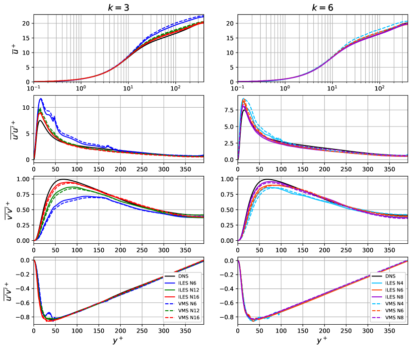
Figure 1. Normalized mean velocity $\overline{u}^{+}$ and normalized Reynolds stresses $\overline{u^{\prime}u^{\prime}}^{+}$, $\overline{v^{\prime}v^{\prime}}^{+}$ and $\overline{u^{\prime}v^{\prime}}^{+}$ over $y^{+}$.

Comparison of HOPU and ILES: As mentioned at the end of section 3.3, one could choose either the standard or the adaptive HOPU method. To motivate the usage of the latter, we plot in figure 2 the absolute value of the average value jump $\eta$ for the channel flow problem using an ILES approach with resolution $N=6/k=3$.

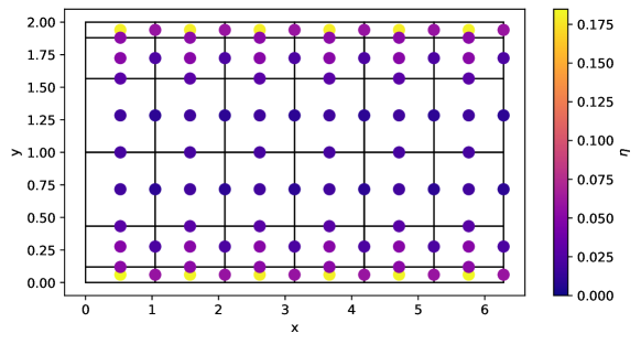
Figure 2. Average absolute value jump $\eta$ for the channel flow problem.

The parameter $\eta$ is averaged over time and in $z$-direction and is visualized in the midpoint of all facets. One observes that $\eta$ is drastically increased close to the lower and upper wall. This motivates to use an adaptive HOPU version with a high-order projection closer to the walls and a low-order projection in the inner region. In figure 3 we again plot $\eta$ but from a different perspective where we also applied an average in $x$-direction. We present the values for an adaptive HOPU approach as motivated above (the exact choice of the local order limits is given below) with the same resolution $N=6/k=3$ (squares) and the ILES from before (circles). We want to emphasize that $\eta$ represents only the high-order part of the averaged jump when using HOPU ($l\geq 0$), but the full average jump for the standard ILES ($\Pi^{l}_{\hat{V}}$ is removed). As we can see, both approximations have roughly the same values in the inner region of the channel. Since in that part of the channel the adaptive HOPU method uses a low-order projection, this is the expected result. Similarly, since a high-order projection is used closer to the wall, we observe a bigger difference of $\eta$ there. This shows, that the amount of additional (numerical) dissipation due to the convection stabilization applied to the highest order functions, is roughly the same in the inner part of the channel, but is reduced closer to the wall when using the HOPU method.

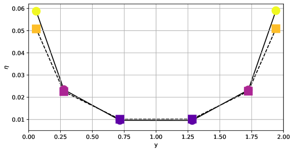
Figure 3. Average absolute value jump $\eta$ at $yz$-facets plotted over $y$ for the ILES (circles) and the HOPU variant (squares).

For the comparison of the velocity profiles and the Reynolds stresses given in figure 4, we have chosen an adaptive HOPU approach with the limits $\eta=\{0.025,0.05,0.1\}$ for $k=3$ and $\eta=\{0.005,0.015,0.03,0.07,0.12,0.2\}$ for $k=6$. A significant improvement of the mean velocity $\overline{u}^{+}$ for the $k=3$ case, especially for $N=6$, is observed for the new method. The HOPU version resolves the buffer region and therefore gives a better approximation of the velocity field in the logarithmic and outer area. The $k=6$ test cases do not show any remarkable differences in the mean velocity and all resolutions give a good prediction of the DNS data. This is because the jumps vanish for highly resolved approximations, and thus naturally removes the additional turbulence model due to HOPU.

For the Reynolds stresses, no significant differences are observed except slight improvements in the near-wall region. A more closed look is given in figure 5. The highly under-resolved $N=6$ and $k=3$ HOPU case shows better agreement of the different moments with the reference data in the proximity of the wall.

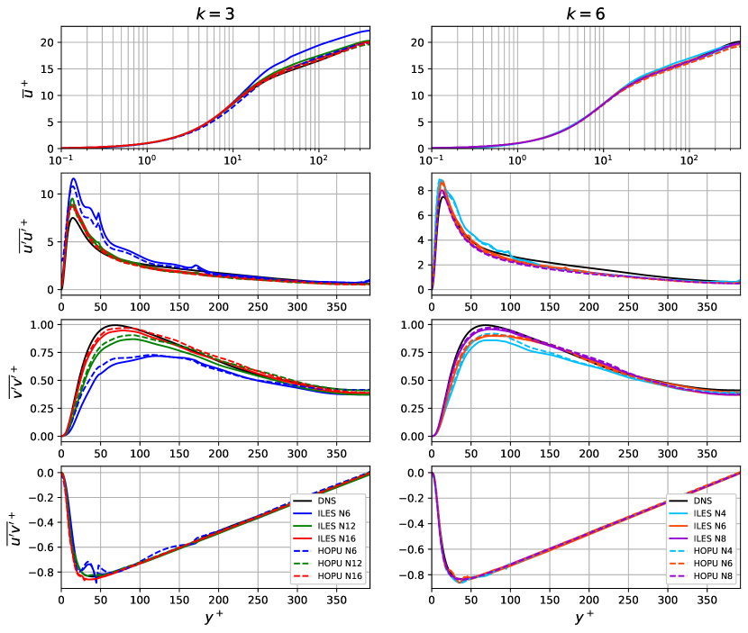
Figure 4. Normalized mean velocity $\overline{u}^{+}$ and normalized Reynolds stresses $\overline{u^{\prime}u^{\prime}}^{+}$, $\overline{v^{\prime}v^{\prime}}^{+}$ and $\overline{u^{\prime}v^{\prime}}^{+}$ over $y^{+}$.

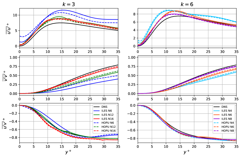
Figure 5. Normalized Reynolds stresses $\overline{u^{\prime}u^{\prime}}^{+}$, $\overline{v^{\prime}v^{\prime}}^{+}$ and $\overline{u^{\prime}v^{\prime}}^{+}$ over $y^{+}$ for the $p=6$ test case.

The relative error between the actual Reynolds number defined by the mean bulk velocity $U_{b}=1/(2\pi)\int_{\partial\Omega|_{x=0}}u\>d\underline{s}$, and the target Reynolds number, can be seen in table 2. Compared to the ILES and VMS simulations, the HOPU variant gives significantly smaller errors in the range of $\leqslant 1\%$ for all resolutions. These results highlight the observations made in figure 1 and 4. It is important to bear in mind that the relative error based on the mean velocity is only a rough error estimation of the approximation.

$N$/$k$	6/3	12/3	16/3
ILES	13.4%	3.1%	1.1%
VMS	16.3%	4.7%	2.7%
HOPU	0.7%	1.0%	0.6%

Table 2. Relative error of the target bulk velocity Reynolds number.

Comparison of the energy spectrum: In figure 6 we compare the methods by its energy spectrum (obtained from the discrete Fourier transformation mentioned before). The time-averaged normalized total energy spectrum $E^{+}$ over the wave number $\kappa$ for the respective approaches is given. Its values are calculated at two different planes normal to the $y$-direction. The first plane is in the viscous sublayer at $y^{+}=5$ and the other one in the buffer layer at $y^{+}=40$. The velocity data for the calculation of the spectrum is provided from a simulation performed with a resolution $N=12$/$k=3$.

In all cases we observe a good approximation of the spectrum in the low-frequent range. As for higher values of $\kappa$, the energy spectrum successively drops as it reaches the dissipative range. The VMS method introduces additional dissipation to the mid to high range. There, the energy spectrum begins to drop at lower wave numbers compared to the ILES approach. Remarkably, the HOPU variant reduces excessive damping and gives a much better prediction of the high wave number range in comparison to the reference DNS data for $y^{+}=5$.

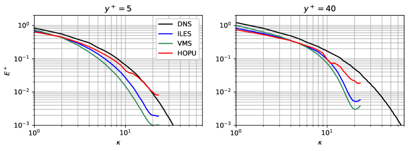
Figure 6. Normalized energy spectrum $E^{+}$ over the wave number $\kappa$ at two different planes, $y^{+}=5$ and $y^{+}=40$ respectively.

5. Periodic hill flow

The prediction of flow quantities from curved surfaces can be assased by the well-known periodic hill flow test case originally proposed in [35]. This type of flow induces several complex flow phenomenons including reattachment, separation and strong interaction with the outer flow. The transition of a boundary layer flow to a separated shear layer can not be predicted by law of the wall and standard model assumptions.

We use the same boundary conditions as for the channel flow. The grid is composed of hexahedral elements that are first stretched with the same stretching function (adapted to the height) as used in section 4, and then curved (using a third order polynomial mapping) to fit the geometry see figure 7. The dimensions of the domain $\Omega=(0,L_{x})\times(0,L_{y})\times(0,L_{z})$ are $L_{x}=9h$, $L_{y}=3.0335h$ and $L_{z}=4.5h$, where $h=1$ denotes the hill height. The characteristic flow is described by the bulk velocity Reynolds number $Re=U_{b}h/\nu$, where the bulk velocity is now given by

$$U_{b}=\frac{1}{(L_{y}-h)L_{z}}\int_{\partial\Omega|_{x=0}}u\>d\underline{s}.$$

In order to obtain a constant bulk velocity Reynolds number (in contrast to a Reynolds number defined with respect to $\tau_{w}$ as for the channel flow) the force on the right hand side is dynamically controlled. For our results, we used $Re=2800$ for all simulations. Two different resolutions are used in this study, which can be seen in table 3. The same time step size is used as for the channel flow. The choice of polynomial order is $k=3$ for both cases.

	$k$	$N_{x}$	$N_{y}$	$N_{z}$	gDOF$\cdot 10^{-3}$
coarse	3	12	8	6	43.2
fine	3	24	16	12	331.0

Table 3. Simulation parameters for the periodic hill flow.

After a statistically-steady state is achieved, the statistical properties at different planes in x-direction are measured over a given time period. The chosen planes are located at $x:\{h,2h,3h,5h,8h\}$. The obtained solutions are compared with the reference DNS data provided by [36].

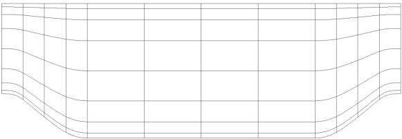
Figure 7. Curvilinear grid for the periodic hill problem.

5.1. Comparison of results

Figure 8 shows the profiles of normalized and averaged velocity components from the different approaches at the considered levels of resolution. The VMS approach uses the order $m=1$ for the space $L_{h}$ and the adaptive HOPU uses the limits $\eta=\{0.025,0.05,0.1\}$. It can be seen that all simulations are able to reproduce the streamwise velocity component $\overline{u}^{+}$ reasonably well. Notable differences are observed in the approximations of $\overline{v}^{+}$. Naturally, the best match with the reference data is obtained for the simulations on the fine grid. In comparison of HOPU to no-model approach, we observe better aggrement of $\overline{v}^{+}$ with HOPU at $x=\{3h,5h,8h\}$ for the coarse mesh. The novel approach shows improved profiles in areas where flow reattachment occurs. The results yielded by the ILES and VMS approaches on the coarse grid are not fundamentally different.

The profiles of the Reynolds stresses can be seen in figure 9. As for the velocities, the solutions accomplished by the finer grid shows overall good agreement in comparison with the reference data. The results obtained by the coarse mesh mostly overestimates the DNS profiles. For the Reynolds stresses $\overline{v^{\prime}v^{\prime}}^{+}$ and $\overline{u^{\prime}v^{\prime}}^{+}$, the HOPU simulation obtains significantly better profiles than the ILES approach. For the VMS approach, only slight to no improvment is observed by the given results.

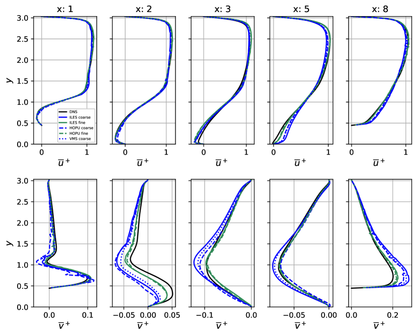
Figure 8. Normalized mean velocity $\overline{u}^{+}$ and $\overline{v}^{+}$ over $y$ at different planes in x-direction.

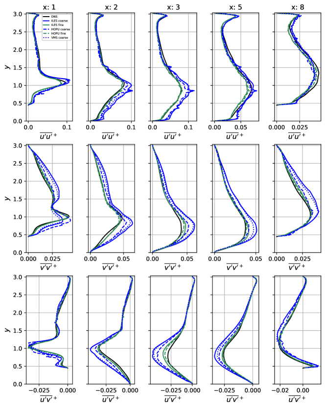
Figure 9. Normalized Reynolds stresses $\overline{u^{\prime}u^{\prime}}^{+}$, $\overline{v^{\prime}v^{\prime}}^{+}$ and $\overline{u^{\prime}v^{\prime}}^{+}$ over $y$ at different planes in x-direction.

The averaged absolute value jump calculated from the coarse ILES simulation is given in figure 10. High values of $\eta$ are observed in the proximity of the lower wall and especially in the downstream region of the hill. Interestingly, the peak value seems to be located in the immediate vicinity of the separation point. This figure gives a rough representation of the areas, which are mostly affected by the HOPU approach.

Figure 10. Average absolute value jump $\eta$ for the periodic hill flow problem.

6. Conclusion

The capacity of the MCS approach to capture structure-resolving turbulent flow in a wall-bounded configuration has been assessed for two different test cases. In addition to the use of a no-model and explicit VMS method, an entirely new technique called high-order projected upwinding, has been introduced to further improve the in-built dissipation capabilites.

In view of the results, we can conclude that the use of a SGS model does not appear to be fundamentally different to the no-model approach. The WALE model incoporated with the VMS approach seems to have an inferior implification on the DG discretization. Furthermore, artificial dissipation introduced by the model can harm the implicit dissipation mechanism and may lead to slightly worse results.
The new high-order projected upwind method significantly improves the results of the standard ILES method for $k=3$ in many areas, especially in the case of the turbulent channel flow. The problem of excessive numerical dissipation introduced by the convection stabilization term in the near-wall region can be avoided by HOPU. It allows for less penalized turbulent transport in this area and overall improved impact on the resolved structures. Results obtained by the discretization using $k=6$ have shown to be not affected considerably by HOPU.

We conclude that the adaptive local order HOPU can be interpreted as a wall model approach for standard DG ILES discretization. However, it is still unclear whether using the absolute value jump as an indicator is the best practice and additional research regarding the adaptivity is needed. However, even in flows where separation appears as in the periodic hill case, HOPU showed an improvement where reattachment appears. By these insights, the novel HOPU method applied to complex turbulent flow problems has to be further investigated in future work.

7. Acknowledgments

This research was funded in part, by the Austrian Science Fund (FWF) [F65-P10 and P35931-N]. For the purpose of open access, the author has applied a CC BY public copyright licence to any Author Accepted Manuscript version arising from this submission.

References

- [1] P. Sagaut and D. Drikakis “Large Eddy Simulation” In Encyclopedia of Aerospace Engineering John WileySons, Ltd, 2010 DOI: https://doi.org/10.1002/9780470686652.eae055
- [2] T. Hughes, L. Mazzei and K. Jansen “Large Eddy Simulation and the variational multiscale method” In Computing and Visualization in Science 3.1, 2000, pp. 47–59 DOI: 10.1007/s007910050051
- [3] P. Fernandez, N. Nguyen and J. Peraire “Subgrid-scale modeling and implicit numerical dissipation in DG-based Large-Eddy Simulation” 23rd AIAA Computational Fluid Dynamics Conference, 2017-3951, 2017 AIAA DOI: 10.1002/fld.4763
- [4] T. Bolemann, A. Beck, D. Flad, H. Frank, V. Mayer and C. Munz “High-Order Discontinuous Galerkin Schemes for Large-Eddy Simulations of Moderate Reynolds Number Flows” In IDIHOM: Industrialization of High-Order Methods - A Top-Down Approach: Results of a Collaborative Research Project Funded by the European Union, 2010 - 2014 Springer International Publishing, 2015, pp. 435–456 DOI: 10.1007/978-3-319-12886-3_20
- [5] S. Collis “Discontinuous Galerkin methods for turbulence simulation” In Studying Turbulence Using Numerical Simulation Databases-IX: Proceedings of the 2002 Summer Program, 2002 URL: https://ntrs.nasa.gov/citations/20030020461
- [6] Marta de la Llave Plata, Vincent Couaillier and M. le Pape “On the use of a high-order discontinuous Galerkin method for DNS and LES of wall-bounded turbulence” In Computers and Fluids 176, 2018, pp. 320–337 DOI: https://doi.org/10.1016/j.compfluid.2017.05.013
- [7] C. Wiart, K. Hillewaert, M. Duponcheel and G. Winckelmans “Assessment of a discontinuous Galerkin method for the simulation of vortical flows at high Reynolds number” In International Journal for Numerical Methods in Fluids 74.7, 2014, pp. 469–493 DOI: https://doi.org/10.1002/fld.3859
- [8] Fan Zhang, Jian Cheng and Tiegang Liu “A high-order discontinuous Galerkin method for the incompressible Navier-Stokes equations on arbitrary grids” In International Journal for Numerical Methods in Fluids 90.5, 2019, pp. 217–246 DOI: https://doi.org/10.1002/fld.4718
- [9] E. Ferrer and R. Willden “A high order Discontinuous Galerkin Finite Element solver for the incompressible Navier–Stokes equations” 10th ICFD Conference Series on Numerical Methods for Fluid Dynamics (ICFD 2010) In Computers and Fluids 46.1, 2011, pp. 224–230 DOI: https://doi.org/10.1016/j.compfluid.2010.10.018
- [10] F. Bassi and S. Rebay “A High-Order Accurate Discontinuous Finite Element Method for the Numerical Solution of the Compressible Navier–Stokes Equations” In Journal of Computational Physics 131.2, 1997, pp. 267–279 DOI: https://doi.org/10.1006/jcph.1996.5572
- [11] N. Fehn, M. Kronbichler, C. Lehrenfeld, G. Lube and P. Schroeder “High-order DG solvers for under-resolved turbulent incompressible flows: A comparison of L2 and H(div) methods” In Numerical Methods in Fluids 91, 2019, pp. 533–556 DOI: 10.1002/fld.4763
- [12] G. Gassner and A. Beck “On the accuracy of high-order discretizations for underresolved turbulence simulations” In Theoretical and Computational Fluid Dynamics 27.3 Springer, 2013, pp. 221–237 DOI: 10.1007/s00162-011-0253-7
- [13] A. Uranga, P. Persson, M. Drela and J. Peraire “Implicit Large Eddy Simulation of transition to turbulence at low Reynolds numbers using a Discontinuous Galerkin method” In International Journal for Numerical Methods in Engineering 87.1-5, 2011, pp. 232–261 DOI: https://doi.org/10.1002/nme.3036
- [14] R. Moura, G. Mengaldo, J. Peiró and S. Sherwin “On the Eddy-Resolving Capability of High-Order Discontinuous Galerkin Approaches to Implicit LES / under-Resolved DNS of Euler Turbulence” In J. Comput. Phys. 330.C USA: Academic Press Professional, Inc., 2017, pp. 615–623 DOI: 10.1016/j.jcp.2016.10.056
- [15] J. Gopalakrishnan, P. Lederer and J. Schöberl “A mass conserving mixed stress formulation for Stokes flow with weakly imposed stress symmetry” In SIAM J. Numer. Anal. 58.1, 2020, pp. 706–732 DOI: 10.1137/19M1248960
- [16] C. Lehrenfeld and J. Schöberl “High order exactly divergence-free Hybrid Discontinuous Galerkin Methods for unsteady incompressible flows” In Computer Methods in Applied Mechanics and Engineering 307, 2016, pp. 339–361 DOI: 10.1016/j.cma.2016.04.025
- [17] J. Schöberl “C++11 Implementation of Finite Elements in NGSolve” In Institute of Analysis and Scientific Computing, Vienna University of Technology, 2014
- [18] P. Raviart and J. Thomas “A Mixed Finite Element Method for Second Order Elliptic Problems” In Mathematical Aspects of Finite Element Methods, Lecture Notes in Mathematics 606, 2006, pp. 292–315 DOI: 10.1007/BFb0064470
- [19] Daniele Boffi, Franco Brezzi and Michel Fortin “Mixed finite element methods and applications” 44, Springer Series in Computational Mathematics Springer, Heidelberg, 2013, pp. xiv+685 DOI: 10.1007/978-3-642-36519-5
- [20] P. Lederer “A Mass Conserving Mixed Stress Formulation for Incompressible Flows” na, 2019
- [21] Jay Gopalakrishnan, Philip Lederer and Joachim Schöberl “A mass conserving mixed stress formulation for the Stokes equations” In IMA J. Numer. Anal. 40.3, 2020, pp. 1838–1874 DOI: 10.1093/imanum/drz022
- [22] Baudouin Veubeke “Discretization of rotational equilibrium in the finite element method” In Mathematical aspects of finite element methods (Proc. Conf., Consiglio Naz. delle Ricerche (C.N.R.), Rome, 1975) Springer, Berlin, 1977, pp. 87–112. Lecture Notes in Math., Vol. 606
- [23] Douglas Arnold, Franco Brezzi and Jim Douglas “PEERS: a new mixed finite element for plane elasticity” In Japan J. Appl. Math. 1.2, 1984, pp. 347–367 DOI: 10.1007/BF03167064
- [24] Rolf Stenberg “A family of mixed finite elements for the elasticity problem” In Numer. Math. 53.5, 1988, pp. 513–538 DOI: 10.1007/BF01397550
- [25] Philip Lederer and Rolf Stenberg “Analysis of Mixed Finite Elements for Elasticity. II. Weak stress symmetry” arXiv, 2022 DOI: 10.48550/ARXIV.2206.14610
- [26] Arnold, D. and Brezzi, F. “Mixed and nonconforming finite element methods : implementation, postprocessing and error estimates” In ESAIM: M2AN 19.1, 1985, pp. 7–32 DOI: 10.1051/m2an/1985190100071
- [27] Lukas Kogler, Philip Lederer and Joachim Schöberl “A conforming auxiliary space preconditioner for the mass conserving mixed stress method” arXiv, 2022 DOI: 10.48550/ARXIV.2207.08481
- [28] George Karniadakis and Spencer Sherwin “Spectral/ element methods for computational fluid dynamics”, Numerical Mathematics and Scientific Computation Oxford University Press, New York, 2005, pp. xviii+657 DOI: 10.1093/acprof:oso/9780198528692.001.0001
- [29] U. Ascher, S. Ruuth and R. Spiteri “Implicit-explicit Runge-Kutta methods for time-dependent partial differential equations” In Applied Numerical Mathematics 25, 1997, pp. 151–167 DOI: 10.1016/S0168-9274(97)00056-1
- [30] B. Pal and S. Ganesan “Projection-based variational multiscale method for incompressible Navier–Stokes equations in time-dependent domains” In International Journal for Numerical Methods in Fluids 84.1, 2017, pp. 19–40 DOI: https://doi.org/10.1002/fld.4338
- [31] V. John and A. Tambulea “On finite element variational multiscale methods for incompressible turbulent flows”, 2006
- [32] F. Ducros, N. Franck and T. Poinsot “Wall-Adapting Local Eddy-Viscosity Models for Simulations in Complex Geometries” In Numerical Methods for Fluid Dynamics VI, 1998
- [33] R. Moura, S. Sherwin and J. Peiró “Linear dispersion–diffusion analysis and its application to under-resolved turbulence simulations using discontinuous Galerkin spectral/hp methods” In Journal of Computational Physics 298, 2015, pp. 695–710 DOI: https://doi.org/10.1016/j.jcp.2015.06.020
- [34] R. Moser, J. Kim and N. Mansour “Direct Numerical Simulation of Turbulent Channel Flow up to Re=590” In Physics of Fluids 11, 1999, pp. 943–945 DOI: 10.1063/1.869966
- [35] C. Mellen, J. Froehlich and W. Rodi “Large eddy simulation of the flow over periodic hills” In 16th IMACS World Congress, Lausanne, Switzerland., 2000
- [36] Ponnampalam Balakumar and George Ilhwan “DNS/LES Simulations of Separated Flows at High Reynolds Numbers” In 45th AIAA Fluid Dynamics Conference DOI: 10.2514/6.2015-2783