Validity in Music Information Research Experiments

Abstract

Validity is the truth of an inference made from evidence, such as data collected in an experiment, and is central to working scientifically. Given the maturity of the domain of music information research (MIR), validity in our opinion should be discussed and considered much more than it has been so far. Considering validity in one’s work can improve its scientific and engineering value. Puzzling MIR phenomena like adversarial attacks and performance glass ceilings become less mysterious through the lens of validity. In this article, we review the subject of validity in general, considering the four major types of validity from a key reference: Shadish et al. [2002]. We ground our discussion of these types with a prototypical MIR experiment: music classification using machine learning. Through this MIR experimentalists can be guided to make valid inferences from data collected from their experiments.

1 Introduction

The multi-disciplinary field of Music Information Research (MIR) is focused on making music and information about music accessible to a variety of users. This ranges from systems for search and retrieval, e.g., Shazam [Wang, 2003] or TunePal [Duggan and O’Shea, 2011], to recommendation, e.g., Spotify or Pandora, and even to more creative applications like generation. These systems consist of many computational components working in domains between the acoustic and symbolic where computability is possible [Müller, 2015]. The effectiveness and reliability of these complex systems and their components are of prime importance to the MIR researcher, not to mention other stakeholders.

The MIR researcher performs experiments to compare approaches for modelling and retrieving music data. A principal focus is on users, but the cost of performing experiments with users is high, and the replicability of such studies is difficult. This has motivated the use of computer-based experiments where “test collections” serve as proxies for human users, known as the Cranfield Paradigm [Cleverdon, 1991]: the researcher predicts the usefulness of an MIR system by applying it to a representative sample of the problem domain (e.g., queries and relevant documents). While such an approach is inexpensive and replicable, its relevance and reliability for MIR, and information retrieval in general, have been questioned [Voorhees, 2001, Urbano et al., 2013].

Under the Cranfield Paradigm, state-of-the-art MIR systems perform exceptionally well in reproducing the ground truth of some datasets, e.g., inferring rhythm, genre or emotion from audio data. However, slight and irrelevant transformations of the audio can suddenly render these systems ineffectual [Sturm, 2014b, Kereliuk et al., 2015, Rodríguez-Algarra et al., 2016, Prinz et al., 2021]. In one case [Rodríguez-Algarra et al., 2016], a “genre recognition” system relies on infrasonic signatures, seemingly originating from the data collection, but nonetheless imperceptible and irrelevant for human listeners. In another case [Sturm et al., 2015], a “rhythm recognition” system seemingly uses tempo to infer rhythm, a confusion originating again from the data collection.

Related are discussions about “glass ceilings” of MIR systems [Aucouturier and Pachet, 2004, Pohle et al., 2008], i.e., that the observed barrier to improving system performance to perfect or human level is due to the psychophysical and cultural factors of music missing from computable features extracted from audio recordings [Wiggins, 2009]. MIR researchers striving for great improvement of those numbers in established problems and datasets might actually make no practical difference for human users [Urbano et al., 2012]. Flexer and Grill [2016] identifies one reason contributing to performance glass ceilings: the data used to train and test MIR systems can arise from tasks that are not well-posed (e.g., music similarity), and thus render meaningless the pursuit of better numbers using that data. The lack of definition in research problems motivates Sturm and Collins [2014] to propose MIR researchers solve synthetic yet well-defined simplifications of harder, ill-posed problems.

At the heart of an MIR experiment is the relationship between conclusions drawn from its results and their validity, or “truth value” [Shadish et al., 2002]. Ideally, an experiment will be carefully designed and implemented to answer a well-defined hypothesis. Its components – units, treatments, design, observations, and settings – should be operationalised (translated from theory into practice) to maximize quality and minimize cost (money, time, ethics). This is the purview of the discipline Design of Experiments: how can one get the best evidence for the least cost? A look through the proceedings of MIR’s premier conference ISMIR and related publications, however, reveals a general lack of awareness of validity in the MIR community.

The first reference explicitly introducing validity to MIR is Urbano [2011], discussing it in relation to text information retrieval (IR) literature, and specifically advocating validity-based meta-evaluation of MIREX results. This is further developed in Urbano et al. [2013], embracing the validity typology of Shadish et al. [2002], and bringing in notions of reliability and efficiency. While the review of Schedl et al. [2013] does not explicitly refer to validity or even mentions the Cranfield Paradigm, it makes clear how central computer experiments are to MIR, and criticizes a general lack of consideration of users in its conclusions. Sturm [2013] asserts that just reporting figures of merit like accuracy is not sufficient to decide whether an MIR system is really recognizing “genre” in musical signals, or whether it relies on irrelevant confounding factors, later stating that these uncontrolled factors are a danger to the validity of conclusions drawn from such experiments [Sturm, 2014b, 2017]. Sturm et al. [2014] attempts to define music description (including the “use case”) to motivate evaluating music description systems in ways that allow for valid and relevant conclusions.

More recently, Rodríguez-Algarra et al. [2019] propose and test a method for detecting the existence of confounding in MIR experiments, thus addressing the lack of construct validity of conclusions drawn from them. Liem and Mostert [2020] studies construct validity of high-level musical concepts like genre by confronting MIR systems with data different from what they have been trained on. Flexer et al. [2021] criticizes the lack of external validity of experiments on general music similarity and demands focus on specific aspects of music similarity and definition of a specific use case. Probably the most recent attempt to comprehensively discuss validity and reliability in MIR is an unpublished tutorial held at ISMIR 2018 [Urbano and Flexer, 2018].

The above review of previous work on validity in MIR shows it to be dispersed and fragmented across only relatively few publications. Despite a small chorus of calls to address major methodological problems of MIR experiments to improve validity in the discipline, e.g., Urbano [2011], Schedl et al. [2013], Sturm [2014b], Urbano and Flexer [2018], Liem and Mostert [2020], Flexer et al. [2021], there has yet to be published a systematic and critical engagement of what validity means in the context of MIR, and how to consider it when designing, implementing and analyzing experiments.

In this article, we review the four principal types of validity in Shadish et al. [2002], an authoritative resource about validity in causal inference and experimental science. Other typologies exist, e.g., Lund [2021], but we focus on that of Shadish et al. [2002] because it is an established point of reference, and has already been introduced to MIR [Urbano et al., 2013]. For each type, we discuss common threats, relate it to the MIR discipline in general, and then more concretely in terms of a typical MIR experiment, presented in Sec. 2. We include a python jupyter notebook that runs the experiment and computes a variety of statistics and results discussed below. Section 3 reviews the components of the experiment, on which the discussion of validity hinges. Each section 4–7 reviews the four types of validity and presents actionable questions which can help MIR researchers to scrutinize the conclusions they draw from their experiments.

2 A Typical MIR Experiment

To ground our general discussion of validity, we present a typical MIR experiment that exemplifies a considerable amount of MIR research: audio classification using machine learning and a benchmark dataset. Consider the BALLROOM dataset [Dixon et al., 2004], created around 2004 from downloading excerpts of music CDs for sale at a website focused on ballroom dancing. BALLROOM consists of 698 audio recordings, each about 30 seconds long and labeled with one of eight dance styles or music rhythms, e.g., “Waltz”. BALLROOM has appeared in dozens of studies [Sturm, 2017], and most often in experiments measuring the amount of ground truth labels reproduced by different combinations of classifiers and features.

We create a random 70/30 partition, with 488/210 recordings comprising the training/testing dataset. From each recording we compute the spectral flux onset strength envelope using a hop size of 1024 samples, or 46 ms [McFee et al., 2015]. We compute the normalised autocorrelation of the envelope and retain the portion relating to lags in $[0.23,4.14]$ seconds. Finally, we model the autocorrelation by a 12th-order autoregressive model, which results in a feature of 13 dimensions describing the 30-second audio recording. We normalise each dimension of the training features to be zero mean and unit variance. We normalise the testing data features using the same parameters as for normalising the training data features.

	Accuracy	Precision	Recall	f1-score
LDA	$0.714$	$0.711$	$0.711$	$0.703$
QDA	$0.719$	$0.715$	$0.723$	$0.717$
1NN	$0.662$	$0.644$	$0.635$	$0.638$
3NN	$0.681$	$0.673$	$0.651$	$0.656$
5NN	$0.719$	$0.699$	$0.687$	$0.689$
7NN	$0.695$	$0.669$	$0.656$	$0.659$
9NN	$0.700$	$0.681$	$0.664$	$0.668$
unif	$0.12\pm 0.02$	$0.13\pm 0.03$	$0.12\pm 0.02$	$0.12\pm 0.02$
freq	$0.13\pm 0.02$	$0.13\pm 0.03$	$0.13\pm 0.02$	$0.13\pm 0.02$
maj	$0.16$	$0.02$	$0.12$	$0.03$

Table 1: Accuracy, and macro-averaged precision, recall and f1-score observed for several models in a testing partition of BALLROOM [Dixon et al., 2004]. The performance of two models randomly selecting labels (with standard deviation) are shown in the rows labeled: unif samples labels uniformly; freq samples labels according to training data label frequency. The last row maj shows the performance of a model choosing the label most frequent in the training data.

We model features using multivariate Gaussian distributions (linear and quadratic discriminant analysis, LDA and QDA), or k-nearest neighbours (KNN). We compare the labels inferred by a model to the ground truth and compute the accuracy, and macro-averaged precision, recall, and f1-score. Table 1 shows the outcomes of this experiment, which can be reproduced with the supplementary python jupyter notebook. The last rows show statistics of three other strategies: unif samples labels according to a uniform prior and freq samples labels according to training data label frequency; maj selects the most frequent label in the training data. These provide comparison points.

A criticism can be made here that the above experiment is not really representative of MIR experiments today: datasets are now several orders of magnitude larger, and deep learning has in many cases made obsolete the engineering of features. However, we will press on with this example for four reasons. First, the BALLROOM dataset is analyzed to such an extent that classification experiments with it illustrate the four types of validity in clear and graspable ways. Using a larger dataset can illustrate the same things, but would first require a thorough analysis of its composition and provenance. Second, concerns about validity are not rendered moot by simply increasing data or shifting the machine learning approach. Third, the experiment above is typical in its design: a dataset is collected and processed, submitted to a variety of machine learning approaches, and measurements are made by applying the trained systems to some test collection. Finally, the BALLROOM dataset is unique in that an “extended” version of it was created a decade later from the same web resource [Marchand and Peeters, 2016]. This allows us to meaningfully test the external validity of conclusions about systems trained in BALLROOM, e.g., the concepts learned from BALLROOM are relevant to ballroom dance music, and not just ballroom dance music in 2004 (see Sec. 7.2).

3 Components of an Experiment

Before discussing the validity of conclusions drawn from the typical MIR experiment, we must identify its units, treatments, design, observations, and settings. Treatments are the things applied to units in order to cause an effect (or not in the case of a control), units are the things that are treated, and observations are what is measured on a unit. The design specifies which treatment is applied to which unit, and settings involve time, place, and condition. To make this more concrete, consider a medical experiment in which the effect of a treatment on blood pressure is being studied. A number of people are sampled from a population, some of whom will receive the treatment while the others receive a placebo (control). The design describes which people get the treatment, and which do not. The observation is the blood pressure of a person after one month. The setting can include particulars of the population (rural or urban), place of treatment (hospital or home), and so on. The experimentalist contrasts blood pressure observations across groups to conclude if the treatment has an effect.

Returning to our typical MIR experiment, we wish to determine the effectiveness of different machine learning (ML) algorithms in predicting the labels of a test recording dataset. There are two possibilities here. We can see the treatments as the ten algorithms, and the units as the entire testing dataset (how does the dataset respond to each algorithm?), or we can see the entire testing dataset as the one treatment, and the units as the ten algorithms (how does each algorithm respond to the dataset?). Since Table 1 reports figures of merit (observations) of each algorithm on the entire dataset, the latter interpretation motivates conclusions about the effectiveness of particular algorithms. In this case, the design is simple: each unit is given the same treatment. The setting involves the partitioning of BALLROOM, the features extracted, random seeds, software libraries, and so on.

4 Statistical Conclusion Validity

Statistical conclusion validity is “the validity of inferences about covariation between two variables” [Shadish et al., 2002]. This includes concluding that a covariation exists, and perhaps its strength as well. This is the level at which one is concerned with statistical significance, i.e., that an observed covariation between treatment and effect is not likely to arise by chance. Shadish et al. [2002] (p. 45) includes a table of nine different threats to statistical conclusion validity. Four threats relevant to computer-based experiments are: violated assumptions about the statistics underlying the responses (and the use of the wrong statistical test, a type III error [Kimball, 1957]); a sample size too small to reliably detect covariation (lack of power); the purposeful search for significant results by trying multiple analyses and data selections (“p-hacking”, Head et al. [2015]); and increased variance in observations due to the heterogeneity of units.

4.1 MIR concerns about statistical conclusion validity

Are my results statistically significant? Null hypothesis statistical testing (NHST) quantifies whether the observed effects of the treatments on the responses arise by mere chance, as well as the direction of effect and its size. This answers the question: are the results statistically significant? Fundamentals about statistical testing in MIR are discussed by Flexer [2006], for Artificial Intelligence in general by Cohen [1995], and for machine learning by Japkowicz and Shah [2011]. One must take care in selecting a statistical test to use; each one makes strong assumptions that could be violated. NHST is most straightforwardly applicable to completely randomized experimental designs [Bailey, 2008], thereby reducing the possibility of structure in units and treatments interfering with the responses (which results in confounding, discussed in the next section). Most MIR experiments cannot use complete randomisation because the target population from which samples come is unclear (what is a random sample of “sad” music, with the term “sad” being quite ill-defined?), and so the kinds of conclusions that can be made with NHST in MIR are limited.

Is the observed statistical significance relevant for a user? In MIR, even if one finds statistical significance, this may not generalise to a perceivable difference for actual users interacting with the “improved” MIR system. As an example from MIR, a crowd-sourced user evaluation [Urbano et al., 2012] demonstrates that there is an upper bound of user satisfaction with music recommendation systems of about $80\%$, since this was the highest percentage of users agreeing that two systems “are equally good.” In addition, for the MIREX task of Audio Music Similarity and Retrieval Urbano et al. [2012] demonstrate that statistically significant differences between algorithms can be so small that they make no practical difference for users.

4.2 Statistical conclusion validity in the typical MIR experiment

Let us now consider the typical MIR experiment in Sec. 2 and reason about what conclusions we can draw from it that have statistical conclusion validity. Table 1 clearly shows that each response of machine learning (ML) to the dataset is greater than the random approaches unif, freq and maj. How likely is it that any of the responses of ML is due to chance, i.e., that any of the ML approaches is actually no better than one of the random approaches? Since we have the empirical distributions for unif and freq, we can estimate the probability of either of them resulting in, e.g., a macro-average recall at least as large as $0.6$: $p<e^{-200}$. Hence, a valid statistical conclusion is that we observe a significant covariation between the use of ML with these particular features and the responses measured on a specific partition of BALLROOM. An equivalent conclusion is that each response of these trained ML systems treated by this partition of BALLROOM are inconsistent with choosing randomly.

Whereas the conclusions above relate to the use of ML, one might consider statistical conclusions relating to the type of ML, i.e., Gaussian modelling (LDA and QDA) vs. nearest neighbour modelling (KNN), or LDA vs. QDA. One may want to conclude that Gaussian modelling is better than nearest neighbour modelling with these features on BALLROOM, or even more precisely, QDA performs the best with these features on BALLROOM. This involves looking at the differences between responses, called contrasts. While there is not much reason to suspect that the particular 70/30 partition of BALLROOM used is unusually beneficial to one kind of ML model over the other, what we do not know from our experiment is the distribution of any response due to ML, and so of any difference of responses due to ML, related to the random partitioning of BALLROOM. We have two measurements of Gaussian models, and five of nearest neighbour models, but we cannot simply compute and compare statistics of these without involving auxiliary information not present in the experiment, e.g., how the decision boundaries of an ML model vary according to variation in the training data.

In fact, if we conclude from Table 1 that Gaussian modelling performs better than nearest neighbour modelling with these features on 70/30 partitions of BALLROOM, we would be wrong. This is a “type I error”, which is concluding there to be a significant difference when in fact there is none. When we perform this experiment 1000 times with random 70/30 partitions we observe that the difference between the best response of a Gaussian model and the best response of a nearest neighbour model is distributed Gaussian, and that the probability of observing zero difference or less is $p>0.41$ for any of the figures of merit (see the accompanying jupyter notebook). That is, the more statistically valid conclusion is that three out of five times randomly partitioning BALLROOM the best Gaussian model performs better than the best nearest neighbor model. With this new data we see that the results in Table 1 do not merit a valid statistical conclusion that one of the modelling approaches is significantly better or worse than any other in BALLROOM using these features for any significance level $\alpha<0.4$. On the other hand, if we were to conclude that QDA performs better than nearest neighbour modelling with these features on 70/30 random partitions of BALLROOM, we would be correct – but only for macro-averaged recall. Performing 1000 repetitions of our experiment shows that the distribution of the difference between the response from QDA and the best response of all others is distributed such that the probability of observing a negative difference is $p<0.046$ only for recall (see the accompanying jupyter notebook). In other words, less than one out of 20 times do we see QDA perform worse than the other models in terms of recall.

In summary, the most general statistical conclusion we can make from Table 1 is that the responses we observe from ML are highly inconsistent with the responses of models choosing randomly. Each ML model knows something about BALLROOM linking the features computed from a music recording with its label. Because we do not know the amount of variation in any response due to partitioning in Table 1, we cannot make any valid statistical conclusion about which type of ML model is the best, or which particular realisation is the best, for this particular dataset. In order to go further, we had to run the experiment multiple times to obtain distributions of the contrasts. Even then, however, we cannot say anything about the cause of significant differences yet. This is where the notion of internal validity becomes relevant.

5 Internal Validity

Internal validity is “the validity of inferences about whether the observed covariation between two variables is causal” [Shadish et al., 2002]. While statistical conclusion validity is concerned only with the strength of covariation between treatment and responses, internal validity is focused on the cause of a particular response to the treatment. Shadish et al. [2002] (p. 55) includes a table of nine different threats to causal conclusions. Several of these involve confounding, which is the confusion of the treatment with other factors arising from poor operationalisation in an experiment.

As a concrete example, consider an experiment measuring the effects of two different medicines on lowering blood pressure, but where one medicine is given to young patients and the other is given to elderly patients. This experimental design confounds the two medicines and patient age, and so the effects caused by the two factors cannot be disambiguated. Any conclusion from this experiment about the effects of the medicines lacks internal validity.

5.1 MIR concerns about internal validity

Does my data collection introduce confounds? One’s methodology for collecting music data might unintentionally introduce structure. For instance, Sturm [2017] discusses how the BALLROOM dataset was assembled by downloading excerpts of music CDs sold at a website selling music for ballroom dance competitions. Ballroom dance competitions are regulated by organisations, e.g., World DanceSport Federation (WDSF), to ensure uniformity of events for competitors around the world. These organisations set strict requirements of tempo of each dance such that high skill is required of the dancers. Hence, the labels of the BALLROOM dataset can mean: 1) the rhythm of the music; 2) the type of dance; 3) the strict tempo requirements of the dance.

Does my data partitioning introduce confounds? Dataset partitioning can also introduce confounds, e.g., “bleeding ground truth.” An example is to first segment recordings into short (e.g., 40ms) time frames and then partition these frames into training and testing sets, thus spreading highly correlated features across these sets. In the context of audio-based genre classification, the presence of songs from the same artists or albums in both training and test data has been shown to artificially inflate performance [Pampalk et al., 2005, Flexer and Schnitzer, 2010]. Flexer [2007] shows that audio-based genre classification using very direct representations of spectral content degrade more when employing artist/album filters than classification based on more abstract kind of features like rhythmic content (fluctuation patterns). This insight that problems of data partitioning can affect MIR systems in quite different ways and hence change performance rankings has been confirmed in another meta-study [Sturm, 2014a].

Research on explainable and interpretable MIR might help to identify confounds, see e.g., [Mishra et al., 2018], but latest results have shown that many popular explainers struggle when being probed with deliberate confounding transformations [Praher et al., 2021, Hoedt et al., 2022b]. A general framework for detecting and characterising effects of confounding in MIR experiments through interventions is proposed by Sturm [2014b] and further refined in Rodríguez-Algarra et al. [2019]. More work has yet to be done in the domain of causal inference in MIR, but is difficult because its core concepts, like “similarity”, need to be operationalised first. Otherwise disentangling variables potentially influencing measurements is not possible.

5.2 Internal validity in the typical MIR experiment

Of interest is what it is in our trained ML models of Sec. 2 causing their response to be inconsistent with random selection. Knowing how Gaussian models used in LDA and QDA are built – mean and covariance parameters are estimated from training data – an internally valid conclusion is that these models work well in BALLROOM because likelihood distributions estimated from the training data also fit the testing data well. Similarly, knowing how nearest neighbour classifiers work, an internally valid conclusion is that in BALLROOM the neighbourhoods of the labeled features in the training data include to a large extent testing data features with the same labels. Another internally valid conclusion is that the high performances of these ML models in BALLROOM are caused by the features together with the expressivity of the models capturing information related to the labels in BALLROOM. Our ML models have learned something about BALLROOM, which causes their performance to be significantly better than random selection.

With reference to the aims of MIR research, we want to conclude something more specific, e.g., our ML models have learned to recognize the rhythms in BALLROOM. This is certainly one explanation consistent with the performance of our systems, but is it the only one? The internal validity of this conclusion relies on a key assumption: inferring the correct labels of BALLROOM can only be the result of learning to discriminate between and identify the rhythms in BALLROOM. In other words, we must assume that there is no other way to accurately infer labels in BALLROOM than by perceiving rhythm.

It is not difficult to imagine other ways to infer the labels in BALLROOM by considering the multitude of variables present in the music recordings. One can hear instrumentation unique to each class, e.g., many recordings labeled “Tango” feature strings, piano and accordion. Many recordings labeled “Waltz” and “Viennese Waltz” feature strings. Many recordings labeled “Quickstep” and “Jive” feature brass, piano, vocals, and drums. So perceiving instrumentation is one way to infer labels in BALLROOM with more success than random selection. We can reject such an explanation knowing that the time-domain nature of the features we are using are not sensitive to timbre, and so cannot clearly express the sound characteristic of an instrument. Then, are there time-domain variables other than rhythm that are closely associated with the labels in BALLROOM?

One possible variable is tempo. If tempo is correlated with rhythm in BALLROOM then tempo estimation is another way a ML model can reproduce the ground truth labels. From listening to BALLROOM recordings labeled “Waltz”, “Quickstep” or “Cha cha cha”, one can hear they feature different rhythms and different tempi, but discriminating between them can be done on the basis of tempo alone. Tempo and rhythm are related musical characteristics, but they are not one and the same thing [Sethares, 2007].

Let us perform an experiment to test the sensitivity of our trained ML models to tempo. We perform an intervention where we alter all test recordings by some amount of pitch-preserving time dilation, and then measure the responses of the models to these new “treatments”. Dilating a recording by an amount 1.1 increases its duration by 10% – or equivalently, makes the music in the recording have a tempo that is 10% slower. Dilating a recording by an amount 0.9 decreases its duration by 10% – or equivalently, makes the music in the recording have a tempo that is 10% faster. Figure 1 shows how the accuracy of all ML models from Table 1 covaries with the amount of dilation. Our intervention has clearly revealed the extent to which the ML models rely on the tempi in the test data – which is no surprise given the background information of BALLROOM in the previous subsection.

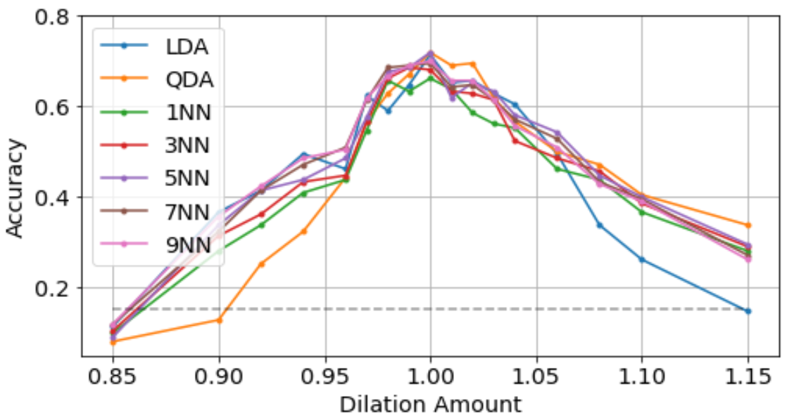
Figure 1: Accuracies of the ML models in Table 1 with test recordings undergoing pitch-preserving time dilation. Horizontal dashed line in grey is the mean accuracy of the best random system plus twice its standard deviation.

The validity of the conclusion that the responses of our ML models are caused by their recognition of the rhythms in BALLROOM relies on too strong of an assumption about BALLROOM, i.e., that rhythm recognition is the only way to infer labels in BALLROOM. The experimental design does not account for the structure present in the dataset; we do not control for other ways of inferring the labels of BALLROOM, which are guaranteed to exist by its very construction. From Table 1 and our experimental design, we thus cannot be any more specific in our causal inference than this: the responses of our ML models are caused by their having learned something about BALLROOM. At best, they are relying on at least tempo and rhythm. This then calls into question how comparing predictions with ground truth in BALLROOM relates to the ability we might actually want to measure, that is the recognition of rhythm. This is where the notion of construct validity becomes relevant.

6 Construct Validity

Construct validity is “the validity of inferences about the higher order constructs that represent sampling particulars” [Shadish et al., 2002]. This involves the relationship between what is meant to be inferred by the experimentalist from an experiment and what is actually measured, i.e., the operationalisation of the experimentalist’s intention. For instance, directly measuring the blood pressure of a person involves an invasive procedure inserting a measuring device in their veins. Blood pressure can be measured less invasively but indirectly by externally applying known pressure to a vein and listening for when blood flow ceases. Knowledge about the incompressibility of liquids in closed systems makes the measurement of pressure in the balloon a relevant measure of blood pressure. Shadish et al. [2002] (p. 73) includes a table of fourteen different threats to construct validity, but several of these are irrelevant to computer-based experiments. The main threat is a questionable relationship between what is being measured and what is intended to be measured. Selecting a measure by convenience but not relevance, sampling from convenient populations, and a lack of definition of what is intended to be measured, are threats to construct validity. Construct validity involves more than just how something is measured; it also involves what is measured and in what settings.

6.1 MIR concerns about construct validity

How is classification accuracy, or any figure of merit, in a labeled music dataset related to X? Two examples in MIR are the use of “genre” classification accuracy as an indirect measure of music similarity [Pohle et al., 2008], or IR user satisfaction (see, e.g., [Schedl et al., 2013] for a discussion). The relationship between these is very tenuous, especially so considering that accuracy itself is an unreliable measure of whether or not a system has learned anything relevant to music [Sturm, 2013, 2014b]. A key reference in this respect is that of Pfungst [1911] describing a series of experiments in trying to reliably measure the arithmetic acumen of a horse that was only able to tap out answers. Counting the number of correct answers tapped out by the horse, no matter how many questions are asked, is irrelevant without considering how each question is posed (the setting). The key to Pfungst discovering the cause of the horse’s apparent arithmetic acumen involved changing the setting: the questions remained the same, and accuracy of correct response was measured, but how the questions were posed was changed in order to control for different factors of the experiment. The same is true for MIR.

What is the “use case” of the system to be tested? To counter threats to construct validity the MIR experimentalist must operationalise as much as possible the use case of the system to be built and tested. An attempt to do so for music description is in Sturm et al. [2014], which emphasises the need to define success criteria. The experimentalist must determine how their method of measurement relates to the success criteria, e.g., relating classification accuracy in BALLROOM to the satisfaction of a specific user.

How can we test the construct validity of a conclusion? One possibility is to assess the outcomes of different experiments which are supposed to measure the same higher order constructs. An example in MIR is to study correlations of different genre classifiers when given identical inputs [Liem and Mostert, 2020]. Low correlations between classifiers point to problems of construct validity. A related topic is that of adversarial examples, which casts doubt on the conclusion that the high accuracy of an MIR system in some dataset reflects its “perception” of the music in the waveform. Adversarial examples have first been described in image analysis [Szegedy et al., 2014], where imperceptible perturbations of input data significantly degraded classification accuracy.

For music genre classification systems, irrelevant audio filtering transformations of music signals are used in Sturm [2014b] to both deflate and inflate classification accuracy to be no better than chance level or perfect $100\%$. The irrelevance is ascertained with listening tests and real human subjects, with the transformation being audible but not changing the clear impression of a certain musical genre. The same problematic behavior has been documented concerning music emotion classification [Sturm, 2014b]. For deep music embedding a test based on imperceptible audio transformations has been proposed [Kim et al., 2019], essentially verifying distance consistency both in the input audio space and corresponding latent deep space.

Following these so-called untargeted attacks which try to change a prediction to an arbitrary target, targeted attacks aiming at changing predictions to specific classes have been explored. A targeted attack on genre recognition has been reported [Kereliuk et al., 2015], where magnitude spectral frames computed from audio are treated as images and attacked using approaches from image object recognition. For music instrument classification a targeted attack allowing to add perturbations directly to audio waveforms instead of spectrograms has also been presented [Prinz et al., 2021]. Quite similar to the results by [Kereliuk et al., 2015], the attacks were able to reduce the accuracy close to a random baseline and produce misclassifications to any desired instrument. Signal perturbations were almost imperceptible apart from some high-frequency deviations. The authors also artificially boosted playcounts via an attack on a real-world music recommender, thereby demonstrating that such attacks can be a security issue in MIR. Follow-up work presented lines of defence against such malicious attacks [Hoedt et al., 2022a].

6.2 Construct validity in the typical MIR experiment

When it comes to our typical MIR experiment in Sec. 2, we are interested in making construct inferences around the latent ability of rhythm recognition we are supposedly measuring. For instance, one construct inference is that our features measure relevant aspects of rhythm in recorded music. In some sense, by their definition from basic signal processing components, our features come from temporal aspects that are certainly relevant to rhythm. Our features are also reliant on acoustic information, and in particular there being high-contrast differences in onsets captured by spectral flux – hence limiting their relationship to rhythms played by particular kinds of instruments with sharp attacks. However, we have seen above that the features are also indicative of tempo, which is not rhythm [Sethares, 2007], and that tempo is another path an ML algorithm can use to get to the rhythm label. Hence we are left to question the relationship of our features to the concept we are trying to operationalise, i.e., rhythm.

The construction of the BALLROOM dataset, intended to reflect different ballroom dance rhythms, is closely related to the validity of construct inferences derived from its use. How do the “Waltz” excerpts exemplify the “Waltz” rhythm? Is there one “Waltz” rhythm? In BALLROOM, there are actually two different labels for waltz: “Waltz” and “Viennese Waltz.” The distinction between them is based in part on tempo, according to the World Sport Dance Federation, a Viennese waltz is to be performed at a tempo between 174-180 BPM Federation [2014].

Having a system label any partition of the BALLROOM dataset provides no reliable measure of a system’s ability to recognise rhythm without changing the setting to control for other factors. It is not as simple as choosing a different feature, measure, cross-validation method, or using a particular statistical test. One must change the experiment itself such that rhythm recognition is what is actually being measured. This means that BALLROOM can still be useful to measuring the rhythm recognition of a ML system. Indeed, in the previous section we used it to disprove the causal claim that the good performance of the ML systems of Table 1 is caused by their ability to recognize rhythm. Might performance in BALLROOM also be an indication of performance in other datasets focused on rhythm? This is where the notion of external validity becomes relevant.

7 External Validity

External validity is “the validity of inferences about the extent to which a causal relationship holds over variations in experimental units, settings, treatment variables and measurement variables” [Shadish et al., 2002]. More generally, external validity is the truth of a generalised causal inference drawn from an experiment. An example is inferring that medicine found to lower blood pressure in patients living in Germany will also lower blood pressure in people living in Mexico – a conclusion that can lack validity due to differences in diet, living and working conditions, and so on. Another example is that increasing the dose of the medicine will cause blood pressure to lower further in the studied population. If a causal inference we draw from an experiment lacks internal validity, then generalising that inference to include variations not tested will not have external validity. Shadish et al. [2002] (p. 87) includes a table of five different threats to external validity, which are in addition to the threats to internal validity. The main threat is that variation of the components of the experiment might destroy the causal inference that holds in the experiment. For instance, a medication may work for the type of illness tested, but that type of illness may not be generalisable to other closely related illnesses.

7.1 MIR concerns about external validity

Does my model generalize to out-of-sample data? The standard approach in evaluating MIR classification systems is to use separate train and test sets in cross-validation experiments to obtain seemingly unbiased estimates of performance. However, if such MIR systems are exposed to independent out-of-sample data often severe loss of performance is observed. One example are experiments on genre recognition where accuracy results do not hold when evaluated across different collections that are not part of the training sets [Bogdanov et al., 2016, 2019]. The results do not generalize to supposedly identical genre labels in different collections, which reflects a lack of external validity. Genre labels like e.g. ’Rock’ will be used differently by different annotators working on these collections – which is a threat to construct validity. Another example are how different audio encodings affect subsequent computation of descriptors and classification results [Urbano et al., 2014], or how in general differences in software implementations diminish replicability [McFee et al., 2018].

Do different raters agree on a ground truth? Human perception of music is highly subjective resulting in possible low inter-rater agreement. Therefore only a certain amount of agreement can be expected if several human subjects are asked to rate the same song pairs according to their perceived similarity, depending on a number of subjective factors [Schedl et al., 2013, Flexer and Grill, 2016] like personal taste, listening history, familiarity with the music, current mood, etc. Concerning annotation of music, Seyerlehner et al. [2010] shows that the performance of humans classifying songs into 19 genres ranges from modest $26\%$ to $71\%$. Audio-based grounding of everyday musical terms shows the same problematic results [Aucouturier, 2009]. It has even been argued [Wiggins, 2009] that no such thing as an immovable ‘ground’ exists in the context of music, because music itself is subjective, highly context-dependent and dynamic.

The lack of inter-rater agreement presents a problem of external validity because inferences from the experiment do not generalize from users or annotators in the experiment to the intended target population of arbitrary users/annotators. It is also a problem of reliability, since different groups of users or annotators with their differing subjective opinions will impede repeatability of experimental results. This lack of inter-rater agreement presents an upper bound for MIR approaches, since it is not meaningful to have computational models going beyond the level of human agreement. Such upper bounds have been reported [Jones et al., 2007, Schedl et al., 2013, Flexer and Grill, 2016] for the MIREX tasks of ‘Audio Music Similarity and Retrieval’ (AMS) and ‘Music Structural Segmentation’ (MSS). For AMS the upper bound has already been reached in 2009, while for MSS the upper bound is within reach for at least some genres of music. Comparable results exist concerning music structure analysis [Nieto et al., 2014] and chord estimation [Ni et al., 2013, Koops et al., 2019].

Do raters agree with themselves at different points in time? Going beyond the question of whether different annotators agree on a ground truth one can also access what the level of agreement within one person is when faced with identical annotation tasks at different points in time. A high intra-rater agreement would help to overcome the problem of upper bounds in MIR systems since it would make personalization of models meaningful, i.e. to have separate models for individual persons. However, at least for the task of general music similarity it has been shown that intra-rater agreement is only slightly higher than inter-rater agreement [Flexer et al., 2021], with the absolute level also depending on music material and mood of raters at test time. An approach to personalize chord labels for individual annotators via deep learning was more successful [Koops et al., 2020].

Returning to the impact of irrelevant transformations [Sturm, 2014b, Kereliuk et al., 2015, Rodríguez-Algarra et al., 2016] and the existence of adversarial examples [Prinz et al., 2021], one can ask, does my model generalize to these kinds of attacks? More constructively, one can seek ways to lessen the impact of these attacks, thus possibly increasing the generalization of the models [Hoedt et al., 2022a].

7.2 External validity in the typical MIR experiment

Considering the typical MIR experiment in Sec. 2, we cannot validly conclude that any of our models is recognizing rhythm in general because we do not know if they are recognizing rhythm in BALLROOM. Our dilation intervention experiment in Sec. 5.2 reveals that all of the models lose their supposed ability to recognize rhythm in BALLROOM, so there is no reason to infer they will recognize rhythm elsewhere. One causal conclusion we might generalise is that all our models perform well in BALLROOM because they have learned something about BALLROOM — a curated set of recordings downloaded from a specific website in 2004. Might our models have also learned something about other recordings from that same website but collected many years later?

The extended BALLROOM dataset (X-BALLROOM) [Marchand and Peeters, 2016] consists of 3,484 audio recordings in the same eight dance styles or music rhythms as BALLROOM, but downloaded from the same website over a decade later. This gives us a chance to test our hypothesis. The figures of merit measured from our models trained in BALLROOM but applied to all of X-BALLROOM are shown in Table 2. We still see significant covariation between response and the use of ML with our features. By and large, whatever concepts our ML models have learned about BALLROOM carry over to X-BALLROOM – but we still do not know whether or not those concepts have to do with rhythm.

	Accuracy	Precision	Recall	f1-score
LDA	$0.659$	$0.647$	$0.643$	$0.643$
QDA	$0.682$	$0.678$	$0.672$	$0.673$
1NN	$0.622$	$0.616$	$0.602$	$0.604$
3NN	$0.636$	$0.629$	$0.610$	$0.613$
5NN	$0.644$	$0.643$	$0.617$	$0.619$
7NN	$0.647$	$0.646$	$0.619$	$0.621$
9NN	$0.645$	$0.643$	$0.615$	$0.618$
unif	$0.12\pm 0.01$	$0.13\pm 0.01$	$0.12\pm 0.01$	$0.12\pm 0.01$
freq	$0.13\pm 0.01$	$0.13\pm 0.01$	$0.12\pm 0.01$	$0.12\pm 0.01$
maj	$0.13$	$0.02$	$0.12$	$0.03$

Table 2: As in Table 1, models trained in BALLROOM and tested in all of X-BALLROOM [Marchand and Peeters, 2016].

We can take this opportunity to test the generalizability of a conclusion about Gaussian modelling outperforming nearest neighbor modelling from Table 1. Training and testing the same ML models with a 70/30 random partition of X-BALLROOM produces the results in Table 3. We still see QDA performing the best, but the nearest neighbor models show large performance increases. The cause of this change in performance should be investigated, and related to the confounding known to exist in BALLROOM. Does the confounding also exist in X-BALLROOM, suggested by the results in Table 2? This shows how the observations made in the typical MIR experiment represent the beginning of avenues for exploration, sources of hypotheses, and not the final result.

Mod	Accuracy	Precision	Recall	f1-score
LDA	$0.726$	$0.721$	$0.722$	$0.717$
QDA	$0.763$	$0.764$	$0.773$	$0.758$
1NN	$0.702$	$0.691$	$0.693$	$0.690$
3NN	$0.741$	$0.731$	$0.727$	$0.727$
5NN	$0.750$	$0.744$	$0.736$	$0.738$
7NN	$0.753$	$0.746$	$0.736$	$0.738$
9NN	$0.751$	$0.746$	$0.734$	$0.737$
unif	$0.12\pm 0.01$	$0.13\pm 0.01$	$0.12\pm 0.01$	$0.12\pm 0.01$
freq	$0.13\pm 0.01$	$0.13\pm 0.01$	$0.13\pm 0.01$	$0.12\pm 0.01$
maj	$0.13$	$0.02$	$0.12$	$0.03$

Table 3: As in Table 1, but models trained and tested in X-BALLROOM [Marchand and Peeters, 2016].

8 Conclusion

This article provides a review of the notion of validity based on the typology given in Shadish et al. [2002]. It brings together the few sources in MIR that mention anything to do with validity, and several sources that do not but are related. This article does not aim to prescribe how to design and perform experiments such that valid conclusions can be drawn from them. Instead it aims to bring within the realm of MIR what validity means, why it is important, and how it can be threatened.

In MIR the predominant experimental methodology is given by the Cranfield paradigm: train a model on a partition of a dataset and count the number of correct answers on another partition. This kind of experiment is inexpensive to do with the data conveniently at hand, and provides numbers that can be compared in ways that convince peer reviewers that progress has been accomplished [Hand, 2006]. Despite various appeals [Peeters et al., 2012, Schedl et al., 2013] and beseechings [Urbano et al., 2012, 2013, Sturm, 2013, 2014b, Flexer and Grill, 2016, Flexer et al., 2021], such an experimental approach is still standard in the field and its serious flaws are ignored. Any inference from this experiment that is more general than “the system has learned something about this dataset” lacks internal, construct and external validity. This does not mean that all such inferences are false, just that they cannot follow from the experiment as designed and implemented. Reproducing the ground truth of a dataset represents a beginning and must be followed by a search for the causes of the observed behavior. One must resist the urge to conclude that a system must be doing whatever is hoped for.

Shadish et al. [2002] provides an established starting point for MIR, but there exist other types of validity. For instance, Lund [2021] revises the typology of Shadish et al. [2002] to address ambiguities between causes and treatments, to better define aspects of settings, and to establish a hierarchical ordering of five types of validity: statistical conclusion, causal, construct, generalization and theoretical. An important distinction in this typology from that of Shadish et al. [2002] is its emphasis on a major aim of basic research: to contribute theory. Other kinds of validity include ecological, convergent, and criterion [Urbano, 2011]; but these still deal with the kind of conclusion one is drawing from evidence collected in some way.

As a final note, a frustration when encountering Shadish et al. [2002] as an engineer is that of its 623 pages there are only five pages with at least one equation on them. Instead, Shadish et al. [2002] describe experiments and how each type of validity manifests in the conclusions drawn, with specific threats to the reasoning of those conclusions. Experiments, not to mention experimentalists, are such complex assemblages that expressing them in formal ways that appear to permit the computation of numbers that relate to each type of validity would probably have very limited applicability, and then only be understood by a limited audience. The language of validity is reason, and we hope this manuscript will inspire MIR researchers to think creatively about the phenomena they observe to discover their causes.

References

- Aucouturier [2009] J.-J. Aucouturier. Sounds like teen spirit: Computational insights into the grounding of everyday musical terms. Language, evolution and the brain, pages 35–64, 2009.
- Aucouturier and Pachet [2004] J.-J. Aucouturier and F. Pachet. Improving timbre similarity: How high is the sky? J. Neg. Results Speech Audio Sci., 1(1):1–13, 2004.
- Bailey [2008] R. A. Bailey. Design of comparative experiments. Cambridge University Press, 2008.
- Bogdanov et al. [2016] D. Bogdanov, A. Porter, H. Boyer, X. Serra, et al. Cross-collection evaluation for music classification tasks. In Proceedings of the 17th International Society for Music Information Retrieval Conference, pages 379 – 385, 2016.
- Bogdanov et al. [2019] D. Bogdanov, A. Porter, H. Schreiber, J. Urbano, and S. Oramas. The acousticbrainz genre dataset: Multi-source, multi-level, multi-label, and large-scale. In Proceedings of the 20th Conference of the International Society for Music Information Retrieval, 2019.
- Chase [2001] A. Chase. Music discriminations by carp “Cyprinus carpio”. Animal Learning & Behavior, 29(4):336–353, 2001.
- Cleverdon [1991] C. W. Cleverdon. The significance of the cranfield tests on index languages. In Proceedings of the 14th annual international ACM SIGIR conference on Research and development in information retrieval, pages 3–12, 1991.
- Cohen [1995] P. R. Cohen. Empirical methods for artificial intelligence, volume 139. MIT press Cambridge, MA, 1995.
- Dixon et al. [2004] S. Dixon, F. Gouyon, and G. Widmer. Towards characterisation of music via rhythmic patterns. In Proceedings of the 5th Conference of the International Society for Music Information Retrieval, pages 509–517, 2004.
- Downie [2006] J. S. Downie. The music information retrieval evaluation exchange (mirex). D-Lib Magazine, 12(12), 2006.
- Duggan and O’Shea [2011] B. Duggan and B. O’Shea. Tunepal: searching a digital library of traditional music scores. OCLC Systems & Services, 27:284–297, 2011.
- Federation [2014] W. S. D. Federation. WSDF Competition Rules. Bucharest, Romania, 2014.
- Flexer [2006] A. Flexer. Statistical evaluation of music information retrieval experiments. Journal of New Music Research, 35(2):113–120, 2006.
- Flexer [2007] A. Flexer. A closer look on artist filters for musical genre classification. In Proceedings the 8th International Conference on Music Information Retrieval, pages 341–344, 2007.
- Flexer and Grill [2016] A. Flexer and T. Grill. The problem of limited inter-rater agreement in modelling music similarity. Journal of new music research, 45(3):239–251, 2016.
- Flexer and Schnitzer [2010] A. Flexer and D. Schnitzer. Effects of album and artist filters in audio similarity computed for very large music databases. Computer Music Journal, 34(3):20–28, 2010.
- Flexer et al. [2021] A. Flexer, T. Lallai, and K. Rašl. On evaluation of inter-and intra-rater agreement in music recommendation. Transactions of the International Society for Music Information Retrieval, 4(1):182–194, 2021.
- Hand [2006] D. J. Hand. Classifier technology and the illusion of progress. Statistical Science, 21(1):1–15, 2006.
- Head et al. [2015] M. L. Head, L. Holman, R. Lanfear, A. T. Kahn, and M. D. Jennions. The extent and consequences of p-hacking in science. PLOS Biology, 13(3):1–15, 2015.
- Hoedt et al. [2022a] K. Hoedt, A. Flexer, and G. Widmer. Defending a Music Recommender Against Hubness-Based Adversarial Attacks. In Proceedings of the 19th Sound and Music Computing Conference, pages 385–390, 2022a.
- Hoedt et al. [2022b] K. Hoedt, V. Praher, A. Flexer, and G. Widmer. Constructing adversarial examples to investigate the plausibility of explanations in deep audio and image classifiers. Neural Computing and Applications, 2022b.
- Japkowicz and Shah [2011] N. Japkowicz and M. Shah. Evaluating Learning Algorithms: A Classification Perspective. Cambridge University Press, New York, NY, USA, 2011.
- Jones et al. [2007] M. C. Jones, J. S. Downie, and A. F. Ehmann. Human similarity judgments: Implications for the design of formal evaluations. In Proceedings of the 8th Conference of the International Society for Music Information Retrieval, pages 539–542, 2007.
- Kereliuk et al. [2015] C. Kereliuk, B. L. Sturm, and J. Larsen. Deep learning and music adversaries. IEEE Transactions on Multimedia, 17(11):2059–2071, 2015.
- Kim et al. [2019] J. Kim, J. Urbano, C. Liem, and A. Hanjalic. Are nearby neighbors relatives? Testing deep music embeddings. Frontiers in Applied Mathematics and Statistics, page 53, 2019.
- Kimball [1957] A. W. Kimball. Errors of the third kind in statistical consulting. J. American Statistical Assoc., 52(278):133–142, June 1957.
- Koops et al. [2019] H. V. Koops, W. B. De Haas, J. A. Burgoyne, J. Bransen, A. Kent-Muller, and A. Volk. Annotator subjectivity in harmony annotations of popular music. Journal of New Music Research, 48(3):232–252, 2019.
- Koops et al. [2020] H. V. Koops, W. B. de Haas, J. Bransen, and A. Volk. Automatic chord label personalization through deep learning of shared harmonic interval profiles. Neural Computing and Applications, 32(4):929–939, 2020.
- Liem and Mostert [2020] C. C. Liem and C. Mostert. Can’t trust the feeling? how open data reveals unexpected behavior of high-level music descriptors. In Proceedings of the 21st International Society for Music Information Retrieval Conference, pages 240–247, 2020.
- Lund [2021] T. Lund. A revision of the campbellian validity system. Scandinavian J. Educational Research, 65(3):523–535, 2021.
- Marchand and Peeters [2016] U. Marchand and G. Peeters. Scale and shift invariant time/frequency representation using auditory statistics: Application to rhythm description. In IEEE International Workshop on Machine Learning for Signal Processing, 2016.
- McFee et al. [2015] B. McFee, C. Raffel, D. Liang, D. P. W. Ellis, M. McVicar, E. Battenberg, and O. Nieto. librosa: Audio and music signal analysis in python. In Proceedings Python in Science Conference, pages 18–25, 2015.
- McFee et al. [2018] B. McFee, J. W. Kim, M. Cartwright, J. Salamon, R. M. Bittner, and J. P. Bello. Open-source practices for music signal processing research: Recommendations for transparent, sustainable, and reproducible audio research. IEEE Signal Processing Magazine, 36(1):128–137, 2018.
- Mishra et al. [2018] S. Mishra, B. L. Sturm, and S. Dixon. Understanding a deep machine listening model through feature inversion. In Proceedings of the 19th International Society for Music Information Retrieval Conference, pages 755–762, 2018.
- Müller [2015] M. Müller. Fundamentals of Music Processing: Audio, Analysis, Algorithms, Applications. Springer, 2015.
- Ni et al. [2013] Y. Ni, M. McVicar, R. Santos-Rodriguez, and T. De Bie. Understanding effects of subjectivity in measuring chord estimation accuracy. IEEE Transactions on Audio, Speech, and Language Processing, 21(12):2607–2615, 2013.
- Nieto et al. [2014] O. Nieto, M. M. Farbood, T. Jehan, and J. P. Bello. Perceptual analysis of the f-measure for evaluating section boundaries in music. In Proceedings of the 15th International Society for Music Information Retrieval Conference, pages 265–270, 2014.
- Pampalk et al. [2005] E. Pampalk, A. Flexer, G. Widmer, et al. Improvements of audio-based music similarity and genre classificaton. In Proceedings of the 6th Conference of the International Society for Music Information Retrieval, pages 634–637, 2005.
- Peeters et al. [2012] G. Peeters, J. Urbano, and G. J. F. Jones. Notes from the ISMIR 2012 late-breaking session on evaluation in music information retrieval. In Proceedings of the 13th Conference of the International Society for Music Information Retrieval, 2012.
- Pfungst [1911] O. Pfungst. Clever Hans (The horse of Mr. Von Osten): A contribution to experimental animal and human psychology. Henry Holt, New York, 1911.
- Pohle et al. [2008] T. Pohle, E. Pampalk, and G. Widmer. Evaluation of frequently used audio features for classification of music into perceptual categories. In International Workshop Content-Based Multimedia Indexing, 2008.
- Praher et al. [2021] V. Praher, K. Prinz, A. Flexer, and G. Widmer. On the Veracity of Local, Model-agnostic Explanations in Audio Classification: Targeted Investigations with Adversarial Examples. In Proceedings of the 22nd International Society for Music Information Retrieval Conference, pages 531–538, 2021.
- Prinz et al. [2021] K. Prinz, A. Flexer, and G. Widmer. On end-to-end white-box adversarial attacks in music information retrieval. Transactions of the International Society for Music Information Retrieval, 4(1):93–104, 2021.
- Rodríguez-Algarra et al. [2016] F. Rodríguez-Algarra, B. L. Sturm, and H. Maruri-Aguilar. Analysing scattering-based music content analysis systems: Where’s the music? In Proceedings of the 17th Conference of the International Society for Music Information Retrieval, pages 344–350, 2016.
- Rodríguez-Algarra et al. [2019] F. Rodríguez-Algarra, B. Sturm, and S. Dixon. Characterising confounding effects in music classification experiments through interventions. Transactions of the International Society for Music Information Retrieval, pages 52–66, 2019.
- Schedl et al. [2013] M. Schedl, A. Flexer, and J. Urbano. The neglected user in music information retrieval research. Journal of Intelligent Information Systems, 41(3):523–539, 2013.
- Sethares [2007] W. A. Sethares. Rhythm and Transforms. Springer, 2007.
- Seyerlehner et al. [2010] K. Seyerlehner, G. Widmer, and P. Knees. A comparison of human, automatic and collaborative music genre classification and user centric evaluation of genre classification systems. In International Workshop on Adaptive Multimedia Retrieval, pages 118–131. Springer, 2010.
- Shadish et al. [2002] W. R. Shadish, T. D. Cook, and D. T. Campbell. Experimental and quasi-experimental designs for generalized causal inference. Boston: Houghton Mifflin, 2002.
- Sturm [2013] B. L. Sturm. Classification accuracy is not enough. Journal of Intelligent Information Systems, 41(3):371–406, 2013.
- Sturm [2014a] B. L. Sturm. The state of the art ten years after a state of the art: Future research in music information retrieval. Journal of New Music Research, 43(2):147–172, 2014a.
- Sturm [2014b] B. L. Sturm. A simple method to determine if a music information retrieval system is a “horse”. IEEE Transactions on Multimedia, 16(6):1636–1644, 2014b.
- Sturm [2017] B. L. Sturm. The “horse” inside: seeking causes behind the behaviors of music content analysis systems. Computers in Entertainment (CIE), 14(2):1–32, 2017.
- Sturm and Collins [2014] B. L. Sturm and N. Collins. The kiki-bouba challenge: Algorithmic composition for content-based mir research & development. In Proceedings of the 15th Conference of the International Society for Music Information Retrieval, pages 21–26, 2014.
- Sturm et al. [2014] B. L. Sturm, R. Bardeli, T. Langlois, and V. Emiya. Formalizing the problem of music description. In Proceedings of the 15th Conference of the International Society for Music Information Retrieval, pages 89–94, 2014.
- Sturm et al. [2015] B. L. Sturm, C. Kereliuk, and J. Larsen. ¿El Caballo Viejo? Latin genre recognition with deep learning and spectral periodicity. In Proceedings of the International Conference on Mathematics and Computation in Music, pages 335–346, 2015.
- Szegedy et al. [2014] C. Szegedy, W. Zaremba, I. Sutskever, J. Bruna, D. Erhan, I. J. Goodfellow, and R. Fergus. Intriguing properties of neural networks. In Proceedings of the 2nd International Conference on Learning Representations, ICLR, 2014.
- Urbano [2011] J. Urbano. Information retrieval meta-evaluation: Challenges and opportunities in the music domain. In Proceedings of the 12th Conference of the International Society for Music Information Retrieval, pages 609–614, 2011.
- Urbano and Flexer [2018] J. Urbano and A. Flexer. Statistical analysis of results in music information retrieval: why and how (abstract). In Proceedings of the International Society for Music Information Retrieval Conference, pages xli–xlii, 2018.
- Urbano et al. [2012] J. Urbano, J. S. Downie, B. Mcfee, and M. Schedl. How significant is statistically significant? the case of audio music similarity and retrieval. In Proceedings of the 13th Conference of the International Society for Music Information Retrieval, pages 181–186, 2012.
- Urbano et al. [2013] J. Urbano, M. Schedl, and X. Serra. Evaluation in music information retrieval. Journal of Intelligent Information Systems, 41(3):345–369, 2013.
- Urbano et al. [2014] J. Urbano, D. Bogdanov, H. Boyer, E. Gómez Gutiérrez, X. Serra, et al. What is the effect of audio quality on the robustness of mfccs and chroma features? In Proceedings of the 15th Conference of the International Society for Music Information Retrieval, pages 573–578, 2014.
- Voorhees [2001] E. M. Voorhees. The philosophy of information retrieval evaluation. In Proceedings of the Cross-Language Evaluation Forum, 2001.
- Wang [2003] A. Wang. An industrial strength audio search algorithm. In Proceedings of the 4th Conference of the International Society for Music Information Retrieval, pages 7–13, Oct. 2003.
- Wiggins [2009] G. A. Wiggins. Semantic gap?? schemantic schmap!! methodological considerations in the scientific study of music. In Proceedings of the 11th IEEE International Symposium on Multimedia, pages 477–482. IEEE, 2009.