Learning Decorrelated Representations Efficiently
Using Fast Fourier Transform

Abstract

Barlow Twins and VICReg are self-supervised representation learning models that use regularizers to decorrelate features. Although these models are as effective as conventional representation learning models, their training can be computationally demanding if the dimension $d$ of the projected embeddings is high. As the regularizers are defined in terms of individual elements of a cross-correlation or covariance matrix, computing the loss for $n$ samples takes $O(nd^{2})$ time. In this paper, we propose a relaxed decorrelating regularizer that can be computed in $O(nd\log d)$ time by Fast Fourier Transform. We also propose an inexpensive technique to mitigate undesirable local minima that develop with the relaxation. The proposed regularizer exhibits accuracy comparable to that of existing regularizers in downstream tasks, whereas their training requires less memory and is faster for large $d$. The source code is available.

1 Introduction

Self-supervised learning (SSL) of representations [29, 4, 30, 16, 5, 14, 6, 33, 1, 11, 34] has become an integral part of deep learning applications in computer vision. Most SSL models for visual representations employ a multi-view, Siamese network architecture. First, an input image is altered by different transformations that preserve its original semantics. The two augmented examples are then fed to a neural network (or in some cases, two different networks) that consists of a backbone network cascaded with a small projection network (usually a multi-layer perceptron) to produce “twin” projected embeddings, or views, of the original. Finally, the network weights are trained so that the twin embeddings (referred to as a “positive pair”) are similar, reflecting the fact that they represent the same original image. After training, the projection network is discarded, while the backbone network is reused for downstream tasks; the idea is that the pretrained backbone should produce generic representations of images that also benefit downstream tasks.

One major issue in SSL is to sidestep collapsed embeddings, or the presence of trivial solutions such that all examples are projected to a single embedding vector. Contrastive approaches [29, 4, 30, 16, 5] eliminate such solutions by a loss term that repels embeddings of different original images (known as “negative pairs”) from each other. Considering all possible negative pairs is infeasible, and negative sampling is usually performed.

Recent studies have explored non-contrastive SSL models. Among these models, Barlow Twins [33] and VICReg [1] use loss functions to penalize features (components of embedding vectors) with a small variance, which are characteristic of collapsed embeddings. Also notable in these loss functions are regularization terms for feature decorrelation. They reduce redundancy in the learned features and make Barlow Twins and VICReg perform as well as contrastive models. However, since the regularizers are defined in terms of elements in a sample cross-correlation or covariance matrix, they require $O(nd^{2})$ time to compute, where $n$ is the number of examples in a batch, and $d$ is the dimensionality of the projected embeddings. This is problematic, as an increased $d$ has been reported to improve the performance of both Barlow Twins and VICReg [33, 1].

Contributions.

We propose a relaxed decorrelating regularizer to address the inefficiency of Barlow Twins and VICReg. The proposed regularizer does not require the explicit calculation of cross-correlation or covariance matrices and can be computed in $O(nd\log d)$ time by means of Fast Fourier Transform (FFT) [8]. Although undesirable local minima develop as a result of relaxation, they can be mitigated by feature permutation; we give an account of why this simple technique works. The SSL models using the proposed regularizer achieve competitive performance with Barlow Twins and VICReg in downstream tasks, with substantially less computation time for large $d$. With $d=8192$, training is 1.2 (with a ResNet-50 backbone) or 2.2 (with a lightweight ResNet-18 backbone) times as fast as Barlow Twins. The proposed method also reduces memory consumption, which allows for larger batch size.

Notation.

We use zero-based indexing for vector and matrix components unless stated otherwise; thus, for a vector $\mathbf{x}\in\mathbb{R}^{d}$, the component index ranges from $0$ to $d-1$. We use $[\mathbf{x}]_{i}$ to denote the $i$th component of vector $\mathbf{x}$, and $[\mathbf{M}]_{ij}$ to denote the $(i,j)$th element of matrix $\mathbf{M}$. For a complex vector $\mathbf{c}$, $\overline{\mathbf{c}}$ denotes its componentwise complex conjugate. For vectors $\mathbf{x}$ and $\mathbf{y}$, $\mathbf{x}\circ\mathbf{y}$ denotes their componentwise product.

2 Related Work

Contrastive SSL.

Contrastive SSL uses positive and negative pairs of augmented samples [29, 4, 30, 16, 5, 10, 7, 26]. The commonly used InfoNCE loss [29] consists of an alignment term, which maximizes the similarity between positive pairs, and a uniformity term, which minimizes the similarity between negative pairs [30]. SimCLR [4] is a state-of-the-art contrastive SSL method. However, to obtain effective representations, SimCLR requires a large number of negative pairs [4], or, in other words, a large batch (or memory bank) size $n$. This can be a computational bottleneck, as the loss computation of SimCLR takes $O(n^{2}d)$ time where $d$ is the dimensionality of the projected embeddings.

Non-contrastive SSL Using Asymmetric Architecture.

Recently, researchers have started exploring non-contrastive approaches to SSL, i.e., those that do not use negative pairs for training. To overcome collapsed embeddings, models such as BYOL [14] and SimSiam [6] introduce asymmetry in the architecture, e.g., by suppressing gradient updates and/or using the moving average of network parameters for one branch of the Siamese network. These methods are heuristically motivated, as collapsed embeddings are not explicitly penalized; however, they are effective in practice.

Non-contrastive SSL by Decorrelating Regularization.

A line of work exists that maintains a standard (symmetric) Siamese network but introduces loss functions to suppress collapsed embeddings. These loss functions also have regularization terms to promote feature decorrelation. Barlow Twins [33] is the first method in this line. It uses a decorrelating regularizer based on cross-correlation across two views. VICReg [1] uses regularizers that are defined in terms of covariance matrices of individual views. We review these methods in detail in Sec. 3.

Non-contrastive SSL by Whitening.

Some authors [11, 19] have used whitening to explicitly decorrelate features during training, as opposed to performing regularization. Subsequent work [34] whitened both features and instances. Because the whitening procedures used in these approaches require the computation of all the eigenvalues of the covariance matrices, a training epoch takes $O(\min(dn^{2},nd^{2}))$ time, which is inefficient with large $d$ or $n$.

Use of Convolution in Machine Learning.

Convolution is the fundamental building block of convolution neural networks (CNNs). CNNs take (linear) convolution of input vectors with small learnable kernels to extract local features. Although FFT reduces the asymptotic complexity of convolution computation, it is seldom used with CNNs, because the size of kernels is typically too small to benefit from speed-up by FFT. In contrast to CNNs, we use (circular) convolution to compute summary statistics of covariance and cross-correlation matrices.

In other areas of machine learning, circular convolution and its non-commutative analogue, circular correlation, have been used for implementing associative memory [3, 24, 22]. The idea has recently been applied to knowledge graph embeddings (KGEs) [20], with the resulting model later shown [15] to be isomorphic to complex-valued KGEs [27] by means of the convolution theorem.

3 SSL Using Decorrelating Regularizers

This section reviews Barlow Twins [33] and VICReg [1]. Given a batch of $n$ original training examples, these models apply two randomly chosen transformations to each example. The transformed examples are then processed independently by a neural network to produce twin embeddings (views) of the original. Let $\mathbf{a}^{(k)},\mathbf{b}^{(k)}\in\mathbb{R}^{d}$ denote the twin embeddings thus obtained for the $k$th example, and let $\mathrm{A}=\{\mathbf{a}^{(k)}\}_{k=1}^{n}$, $\mathrm{B}=\{\mathbf{b}^{(k)}\}_{k=1}^{n}$ be the sets of embeddings for individual views. Given these embeddings, the network is trained to minimize the loss function specific to each model.

Barlow Twins.

Barlow Twins optimizes the loss function defined in terms of the cross-correlation matrix $\mathbf{C}(\mathrm{A},\mathrm{B})\in\mathbb{R}^{d\times d}$ between views $\mathrm{A}$ and $\mathrm{B}$:

$$L_{\textup{BT}} =\sum_{i=0}^{d-1}\left(1-[\mathbf{C}(\mathrm{A},\mathrm{B})]_{ii}\right)^{2}+\lambda R_{\textup{off}}(\mathbf{C}(\mathrm{A},\mathrm{B})),$$ (1)

where hyperparameter $\lambda\geq 0$ controls the strength of regularization, and $R_{\textup{off}}:\mathbb{R}^{d\times d}\to\mathbb{R}$ is a regularizer function defined as

$$R_{\textup{off}}(\mathbf{M}) =\sum_{i=0}^{d-1}\sum_{\begin{subarray}{c}j=0\\ j\neq i\end{subarray}}^{d-1}[\mathbf{M}]_{ij}^{2}.$$ (2)

The first term in Eq. 1 is minimized when the corresponding features of two views are fully correlated, i.e., $[\mathbf{C}(\mathrm{A},\mathrm{B})]_{ii}=1$ for $i=0,\dots,d-1$. This term can be efficiently computed in $O(nd)$ time. Regularizer $R_{\textup{off}}(\mathbf{C}(\mathrm{A},\mathrm{B}))$ in the second term is responsible for feature decorrelation, as it is minimized when all the off-diagonal elements in $\mathbf{C}(\mathrm{A},\mathrm{B})$ are zero. For a large $d$, $R_{\textup{off}}(\mathbf{C}(\mathrm{A},\mathrm{B}))$ can be a computational burden, as it takes $O(nd^{2})$ time to compute due to the $d\times d$ matrix $\mathbf{C}(\mathrm{A},\mathrm{B})$.

VICReg.

Let $\mathbf{K}(\mathrm{A}),\mathbf{K}(\mathrm{B})\in\mathbb{R}^{d\times d}$ be the covariance matrices of $\mathrm{A}$ and $\mathrm{B}$, respectively. The VICReg loss function is

$$L_{\textup{VIC}} =\frac{\alpha}{n}\sum_{k=1}^{n}\|\mathbf{a}^{(k)}-\mathbf{b}^{(k)}\|^{2}_{2}$$

$$\quad+\frac{\mu}{d}\left(R_{\textup{var}}(\mathbf{K}(\mathrm{A}))+R_{\textup{var}}(\mathbf{K}(\mathrm{B}))\right)$$

$$\quad+\frac{\nu}{d}\left(R_{\textup{off}}(\mathbf{K}(\mathrm{A}))+R_{\textup{off}}(\mathbf{K}(\mathrm{B}))\right),$$ (3)

where hyperparameters $\alpha,\mu,\nu\geq 0$ control the importance of individual terms, and $R_{\textup{var}}$ is the regularizer defined as

$$R_{\textup{var}}(\mathbf{M}) =\sum_{i=0}^{d-1}\text{max}(0,\gamma-\sqrt{[\mathbf{M}]_{ii}}),$$ (4)

with the target standard deviation $\gamma>0$. Function $R_{\textup{off}}$ is the same regularizer as used in Barlow Twins (Eq. 2), but here, it is applied to $\mathbf{K}(\mathrm{A})$ and $\mathbf{K}(\mathrm{B})$ instead of $\mathbf{C}(\mathrm{A},\mathrm{B})$.

The first term in Eq. 3 brings two embeddings of the same example closer. Regularizer $R_{\textup{var}}$ penalizes collapsed embeddings with zero variance, whereas $R_{\textup{off}}$ promotes the diversity of features by encouraging the feature covariance to be zero. The time complexity of calculating $R_{\textup{off}}(\mathbf{K}(\mathrm{A}))$ and $R_{\textup{off}}(\mathbf{K}(\mathrm{B}))$ is $O(nd^{2})$, identical to that of $R_{\textup{off}}(\mathbf{C}(\mathrm{A},\mathrm{B}))$ in Barlow Twins.

4 Proposed Method

We propose a weaker but efficiently computable alternative to the regularizer function $R_{\textup{off}}$. In the following, our regularizer is presented in terms of cross-correlation matrix $\mathbf{C}(\mathrm{A},\mathrm{B})$, similarly to Barlow Twins. However, if applied instead to $\mathbf{K}(\mathrm{A})$ and $\mathbf{K}(\mathrm{B})$, it produces a relaxed version of the corresponding regularization terms in the VICReg loss.

4.1 Regularizer Based on Sums of Cross-correlations

Recall that the Barlow Twins loss is based on the cross-correlation matrix $\mathbf{C}=\mathbf{C}(\mathrm{A},\mathrm{B})$ of two views $\mathrm{A}=\{\mathbf{a}^{(k)}\}_{k=1}^{n}$ and $\mathrm{B}=\{\mathbf{b}^{(k)}\}_{k=1}^{n}$. For brevity, assume that both $A$ and $B$ are standardized. Then, we can simply write $\mathbf{C}=(1/(n-1))\sum_{k=1}^{n}\mathbf{a}^{(k)}{\mathbf{b}^{(k)}}^{\textup{T}}$.

Our regularizer is defined in terms of a $d$-dimensional “summary” vector of the $d\times d$ matrix $\mathbf{C}$. This vector, denoted by $\mathop{\textup{sumvec}}(\mathbf{C})$, is given componentwise by

$$\left[\mathop{\textup{sumvec}}(\mathbf{C})\right]_{i} =\sum_{j=0}^{d-1}[\mathbf{C}]_{j,(i+j)\bmod d}.$$ (5)

Note the zero-based component indices. The zeroth component $[\mathop{\textup{sumvec}}(\mathbf{C})]_{0}$ is the trace of $\mathbf{C}$. Each of the remaining $d-1$ components corresponds to a sum of $d$ different off-diagonal elements of $\mathbf{C}$, with no single element appearing in two distinct sums. Thus, every element in $\mathbf{C}$ appears exactly once in the summations in Eq. 5. The calculation of a summary vector for a $3\times 3$ covariance matrix is illustrated in Fig. 1.

$\left\{\;\begin{aligned} v_{0}&=c_{00}+c_{11}+c_{22}\\ v_{1}&=c_{01}+c_{12}+c_{20}\\ v_{2}&=c_{02}+c_{10}+c_{21}\end{aligned}\right.$

Figure 1: A $3\times 3$ cross-correlation matrix $\mathbf{C}=\left[c_{ij}\right]$ ($i,j=0,1,2$) and $\mathop{\textup{sumvec}}(\mathbf{C})=[v_{0}\;v_{1}\;v_{2}]^{\textup{T}}$.

Now, we define a regularizer in terms of all but the zeroth component of $\mathop{\textup{sumvec}}(\mathbf{C})$:

$$R_{\textup{sum}}(\mathbf{C})=\sum_{i=1}^{d-1}\|[\mathop{\textup{sumvec}}(\mathbf{C})]_{i}\|_{q}^{q},$$ (6)

where hyperparameter $q\in\{1,2\}$. This function $R_{\textup{sum}}$ can be used as a drop-in replacement for $R_{\textup{off}}$ in the Barlow Twins loss (Eq. 1). The zeroth component $[\mathop{\textup{sumvec}}(\mathbf{C})]_{0}$ is excluded in Eq. 6, because it concerns the diagonal elements of $\mathbf{C}$ that are irrelevant to feature decorrelation; they do not appear in Barlow Twin’s regularizer $R_{\textup{off}}(\mathbf{C})$ either.

The regularizer $R_{\textup{sum}}$ is weaker than $R_{\textup{off}}$ in that it imposes constraints on the components of the summary vector, or the sums of $d$ elements of $\mathbf{C}$, whereas $R_{\textup{off}}$ constrains individual elements. Indeed, the minimizers of $R_{\textup{off}}(\mathbf{C})$ also minimize $R_{\textup{sum}}(\mathbf{C})$, but the converse does not necessarily hold. However, as we discuss in Sec. 4.2, $R_{\textup{sum}}$ allows faster computation. Furthermore, in Sec. 4.3, we provide a simple technique to mitigate the weakness of $R_{\textup{sum}}$.

4.2 Efficient Computation

Computing $\mathop{\textup{sumvec}}(\mathbf{C})$ by Eq. 5 requires the cross-correlation matrix $\mathbf{C}(\mathrm{A},\mathrm{B})$, whose calculation incurs the same computational cost as that of the Barlow Twins loss. However, by means of the Fourier transform, $\mathop{\textup{sumvec}}(\mathbf{C})$ can be calculated directly from the vectors in $\mathrm{A}$ and $\mathrm{B}$ without explicit calculation of their cross-correlation matrix. To this end, we use involution and circular convolution.

For a vector $\mathbf{x}\in\mathbb{R}^{d}$, its involution [24] (also called flipping [25]) $\mathop{\textup{inv}}(\mathbf{x})$ is the vector obtained by reversing the order of its first (not the zeroth) to $(d-1)$st components; i.e., $[\mathop{\textup{inv}}(\mathbf{x})]_{i}=[\mathbf{x}]_{(d-i)\bmod d}$ for $i=0,\ldots,d-1$.

For vectors $\mathbf{x},\mathbf{y}\in\mathbb{R}^{d}$, their circular convolution $\mathbf{x}*\mathbf{y}$ is a $d$-dimensional vector with components given as

$$\left[\mathbf{x}*\mathbf{y}\right]_{i} =\sum_{j=0}^{d-1}\left[\mathbf{x}\,\mathbf{y}^{\textup{T}}\right]_{j,(i-j)\bmod d}.$$ (7)

As a result, circular convolution is known as the “compressed outer product.”

Now, for each twin embedding pair $\mathbf{a}^{(k)}\in\mathrm{A}$ and $\mathbf{b}^{(k)}\in\mathrm{B}$ ($k=1,\ldots,n$), let us consider vector $\mathop{\textup{inv}}(\mathbf{a}^{(k)})*\mathbf{b}^{(k)}\in\mathbb{R}^{d}$. Noting the indices altered by involution, we see that this vector is given componentwise by

$$\left[\mathop{\textup{inv}}(\mathbf{a}^{(k)})*\mathbf{b}^{(k)}\right]_{i} =\sum_{j=0}^{d-1}\left[\mathbf{a}^{(k)}{\mathbf{b}^{(k)}}^{\textup{T}}\right]_{j,(i+j)\bmod d}.$$ (8)

Substituting $\mathbf{C}=(1/(n-1))\sum_{k=1}^{n}\mathbf{a}^{(k)}{\mathbf{b}^{(k)}}^{\textup{T}}$ into Eq. 5 and using Eq. 8, we have

$$\left[\mathop{\textup{sumvec}}(\mathbf{C})\right]_{i} =\sum_{j=0}^{d-1}{\overbrace{\left[\frac{1}{n-1}\sum_{k=1}^{n}\mathbf{a}^{(k)}{\mathbf{b}^{(k)}}^{\textup{T}}\right]}^{\mathbf{C}}}_{j,(i+j)\bmod d}$$

$$=\frac{1}{n-1}\sum_{k=1}^{n}\sum_{j=0}^{d-1}\left[\mathbf{a}^{(k)}{\mathbf{b}^{(k)}}^{\textup{T}}\right]_{j,(i+j)\bmod d}$$

$$=\frac{1}{n-1}\sum_{k=1}^{n}\left[\mathop{\textup{inv}}(\mathbf{a}^{(k)})*\mathbf{b}^{(k)}\right]_{i},$$ (9)

or, as a vector,

$$\mathop{\textup{sumvec}}(\mathbf{C}) =\frac{1}{n-1}\sum_{k=1}^{n}\mathop{\textup{inv}}(\mathbf{a}^{(k)})*\mathbf{b}^{(k)}.$$ (10)

Let $\mathop{\mathscr{F}}$ and $\mathop{\mathscr{F}^{-1}\!}$ denote the discrete Fourier transform and inverse discrete Fourier transform, respectively. Noting that $\mathop{\mathscr{F}}(\mathop{\textup{inv}}(\mathbf{x}))=\overline{\mathop{\mathscr{F}}(\mathbf{x})}$ for any $\mathbf{x}\in\mathbb{R}^{d}$ (see e.g., [25], Section 7.4.2) and using the convolution theorem $\mathop{\mathscr{F}}(\mathbf{x}*\mathbf{y})=\mathop{\mathscr{F}}(\mathbf{x})\circ\mathop{\mathscr{F}}(\mathbf{y})$, we have

$$\mathop{\textup{inv}}(\mathbf{a}^{(k)})*\mathbf{b}^{(k)} =\mathop{\mathscr{F}^{-1}\!}\left(\overline{\mathop{\mathscr{F}}(\mathbf{a}^{(k)})}\circ\mathop{\mathscr{F}}(\mathbf{b}^{(k)})\right).$$ (11)

Substituting Eq. 11 into Eq. 10, we obtain

$$\mathop{\textup{sumvec}}(\mathbf{C}) =\frac{1}{n-1}\sum_{k=1}^{n}\overbrace{\mathop{\mathscr{F}^{-1}\!}\left(\overline{\mathop{\mathscr{F}}(\mathbf{a}^{(k)})}\circ\mathop{\mathscr{F}}(\mathbf{b}^{(k)})\right)}^{\mathop{\textup{inv}}(\mathbf{a}^{(k)})*\mathbf{b}^{(k)}}$$

$$=\frac{1}{n-1}\mathop{\mathscr{F}^{-1}\!}\left(\sum_{k=1}^{n}\overline{\mathop{\mathscr{F}}(\mathbf{a}^{(k)})}\circ\mathop{\mathscr{F}}(\mathbf{b}^{(k)})\right).$$ (12)

Using this equation, we can compute $\mathop{\textup{sumvec}}(\mathbf{C})$ directly from the embedding vectors $\{\mathbf{a}^{(k)},\mathbf{b}^{(k)}\}_{k=1}^{n}$, bypassing the cumbersome calculation of $\mathbf{C}$. Noting that the (inverse) Fourier transform of a $d$-dimensional vector can be performed in $O(d\log d)$ time by the FFT algorithm, while the calculation of complex conjugates, component products, and the sum of $n$ vectors takes $O(nd)$ time, we can see that the overall time to obtain $\mathop{\textup{sumvec}}(\mathbf{C})$ is $O(nd\log d)$, which is also the time needed to compute $R_{\textup{sum}}(\mathbf{C})$. This is a substantial improvement over the $O(nd^{2})$ computation time of $R_{\textup{off}}(\mathbf{C})$ in the Barlow Twins loss.

Furthermore, the space complexity of computing $R_{\textup{sum}}(\mathbf{C})$ is $O(nd)$, which is optimal if the $O(nd)$ space needed to store input vectors $\mathrm{A}$ and $\mathrm{B}$ is considered as part of the complexity. In contrast, Barlow Twins requires extra $O(d^{2})$ space to store $\mathbf{C}$.

4.3 Feature Permutation to Mitigate Undesirable Local Minima

As seen from Eq. 5, the components of $\mathop{\textup{sumvec}}(\mathbf{C})$ are the sums of $d$ elements in $\mathbf{C}$, and the proposed regularizer $R_{\textup{sum}}$ (Eq. 6) encourages these sums to be close to zero. This is weaker than the regularizer $R_{\textup{off}}$ (Eq. 2) in the Barlow Twins loss, which pushes individual elements of $\mathbf{C}$ towards zero. Indeed, $R_{\textup{sum}}(\mathbf{C})$ can be close to zero even if individual elements in $\mathbf{C}$ are not; the summands in Eq. 5 can cancel each other, since they can be either positive or negative. As a result, undesirable local minima develop in the parameter space, rendering our regularizer ineffective.

Here, we propose a technique to eliminate these local minima: we randomly permute feature indices during training so that sums of different cross-correlation terms constitute $\mathop{\textup{sumvec}}(\mathbf{C})$. To understand why this simple technique is effective, consider minimizing $R_{\textup{sum}}(\mathbf{C})$, regarding the elements of $\mathbf{C}$ as independent variables. It is easy to see that the minimum is attained by the solutions to a homogeneous system of linear equations:

$$\overbrace{\sum_{j=0}^{d-1}[\mathbf{C}]_{j,(i+j)\bmod d}}^{\left[\mathop{\textup{sumvec}}(\mathbf{C})\right]_{i}} =0,\qquad\text{for }i=1,\ldots,d-1.$$

This is an underdetermined system, with only $d-1$ equations but with $d(d-1)$ unknowns, namely, $[\mathbf{C}]_{j\ell}$, $j,\ell=0,\ldots,d-1,j\neq\ell$. This underdeterminacy is the cause of nontrivial solutions such that $[\mathbf{C}]_{j\ell}\neq 0$, that is, undesirable solutions in which summands with opposite signs cancel each other in an equation.

Now, by repeatedly permuting the feature indices and minimizing the loss, we effectively introduce additional equations to the system, since permutation can produce different sets of linear equations over the unknowns, and these new constraints eventually render nontrivial solutions inadmissible.

For ease of implementation, we permute feature indices randomly during training, instead of generating all permutations systematically at once, similarly to the way that stochastic gradient descent is a modification to full gradient descent. Note that the permuted feature indices need not be identical across mini-batches, even within a single epoch; indeed, in the experiments presented in Sec. 5, we use a different random permutation of features in every mini-batch in every epoch.

4.4 Feature Grouping to Control the Degree of Relaxation

Instead of computing a summary vector for an entire cross-correlation matrix $\mathbf{C}$, we can compute summaries at a more fine-grained level. Specifically, we partition $d$ features into groups of size $b$ each. This partitioning induces in $\mathbf{C}$ a total of $\lceil d/b\rceil^{2}$ block submatrices of size $b\times b$, i.e., $\mathbf{C}=[\mathbf{C}_{ij}]$ $(i,j=1,\ldots,\lceil d/b\rceil)$ with submatrices $\mathbf{C}_{ij}\in\mathbb{R}^{b\times b}$. We then define the regularizer as

$$R_{\textup{sum}}^{(b)}(\mathbf{C}) =\sum_{i=1}^{\lceil d/b\rceil}\sum_{\ell=1}^{b-1}\left\|[\mathop{\textup{sumvec}}(\mathbf{C}_{ii})]_{\ell}\right\|_{q}^{q}$$

$$\qquad+\sum_{\begin{subarray}{c}i,j=1\\ i\neq j\end{subarray}}^{\lceil d/b\rceil}\sum_{\ell=0}^{b-1}\left\|[\mathop{\textup{sumvec}}(\mathbf{C}_{ij})]_{\ell}\right\|_{q}^{q}.$$ (13)

As before, $\mathop{\textup{sumvec}}(\mathbf{C}_{ij})$ can be computed without explicitly computing $\mathbf{C}_{ij}$ by means of involution, circular convolution (of subvectors of embeddings), and the Fourier transform. Calculating a single $\mathop{\textup{sumvec}}(\mathbf{C}_{ij})$ takes $O(nb\log b)$ time using FFT, and since there are $\lceil d/b\rceil^{2}$ blocks, the total time needed to compute $R_{\textup{sum}}^{(b)}$ is $O((nd^{2}/b)\log b)$.

The block size hyperparameter $b$ controls the granularity of the summary computation and interpolates the proposed and existing regularizers. On one hand, the regularizer $R_{\textup{sum}}^{(1)}(\mathbf{C})$ reduces $R_{\textup{off}}(\mathbf{C})$ of Barlow Twins when $b=1$, provided that $q=2$. On the other hand, when $b=d$, we recover $R_{\textup{sum}}^{(d)}(\mathbf{C})=R_{\textup{sum}}(\mathbf{C})$ given in Eq. 6. Thus, this grouping formulation provides a generalization of Barlow Twins, with parameter $b$ controlling the trade-off between the computational efficiency and the degree of relaxed regularization. Empirically, the performance can be slightly improved by the use of a feature group of moderate size, with no substantial degradation observed in training time and memory usage; see Sec. 5.

It should be noted that the permutation and grouping of features are compatible and can be combined.

4.5 Regularizer Based on Sums of Feature Covariances

The function $R_{\textup{sum}}$ can also be used to define a VICReg-style regularizer based on covariance, simply by replacing $R_{\textup{off}}$ with $R_{\textup{sum}}$ in Eq. 3, and passing correlation matrices $\mathbf{K}(\mathrm{A})$ or $\mathbf{K}(\mathrm{B})$ instead of $\mathbf{C}(\mathrm{A},\mathrm{B})$ as the argument. Fast computation is possible with FFT, and the grouping version is also straightforward; this is described in greater detail in Supplementary Material.

4.6 Summary of Proposed Models

The loss functions of the proposed models are summarized below. Let the function $R=R_{\textup{sum}}^{(b)}$ if feature grouping is used with block size $b$, or let $R=R_{\textup{sum}}$ if grouping is not used.

For Barlow Twins-style cross-correlation regularization, the loss function is

$$L =\sum_{i}\left(1-[\mathbf{C}(\mathrm{A},\mathrm{B})]_{ii}\right)^{2}+\lambda R(\mathbf{C}(\mathrm{A},\mathrm{B})),$$ (14)

whereas for VICReg-style covariance regularization, we use

$$L =\frac{\alpha}{n}\sum_{i}\|\mathbf{a}^{(i)}-\mathbf{b}^{(i)}\|^{2}_{2}+\frac{\mu}{d}\left(R_{\textup{var}}(\mathbf{K}(\mathrm{A}))+R_{\textup{var}}(\mathbf{K}(\mathrm{B}))\right)$$

$$\qquad+\frac{\nu}{d}\left(R(\mathbf{K}(\mathrm{A}))+R(\mathbf{K}(\mathrm{B}))\right).$$ (15)

Setting $R=R_{\textup{off}}$ in these formulas gives the original Barlow Twins and VICReg, when hyperparameter $q=2$.

5 Experiments

We empirically evaluate the effect of the proposed regularizers. To be precise, we train SSL models using the Barlow Twins–style loss function of Eq. 14 and the VICReg-style loss function of Eq. 15 and compare their performance with Barlow Twins and VICReg in downstream tasks. The training time and memory consumption are also evaluated. For our models, feature permutation is performed in every batch iteration except for the ablation study.

In the following, we briefly present the tasks and datasets used in the experiments. See Appendices D and E for the complete experimental setup, including the hyperparameter values and the results of additional experiments.

5.1 Tasks and Datasets

Models are pretrained with images in the ImageNet dataset [9] or its subset, ImageNet-100 [26], depending on the experiment. ResNet-50 [17] is used as the backbone for ImageNet, while ResNet-18 is used for ImageNet-100.

To evaluate downstream SSL performance, we follow the standard linear evaluation protocol: After the backbone network is pretrained by a SSL method, we train a linear classifier on top of the frozen backbone using labeled data from the ImageNet or ImageNet-100 training set. The resulting classifier is then evaluated by the top-1 and top-5 accuracy on the respective validation sets.

For transfer learning evaluation, we apply the pretrained models to an object detection task on Pascal VOC07+12 [12]. Following previous studies [16, 33, 1], we use the trainval set of VOC2007 and VOC2012 for training and the test split of VOC2007 for testing. We fine-tune Faster R-CNN [23] with R50-C4. Models are evaluated by three types of average precision (AP): AP, $\text{AP}_{50}$, and $\text{AP}_{75}$, where $\text{AP}_{x}$ signifies the intersection-over-union (IoU) threshold of $x$ %. We report the average scores over five trials.

5.2 Results and Discussion

Table 1: Linear evaluation accuracy (%) on ImageNet-100 with $d=2048$. Bold numbers indicate the best performance within each family (cross-correlation regularization, covariance regularization, or other SSL models). ${\dagger}$: quoted from the solo-learn [28] GitHub repository as of December 28, 2022; ${\ddagger}$: quoted from [34].

Model	Top-1	Top-5
Barlow Twins†	80.16	95.14
Barlow Twins	80.12	95.24
Proposed (Barlow Twins–style; no grouping)	79.94	94.76
Proposed (Barlow Twins–style; $b=128$)	81.02	95.24
VICReg†	79.40	95.02
VICReg	79.30	94.30
Proposed (VICReg-style; no grouping)	79.20	94.96
Proposed (VICReg-style; $b=128$)	80.04	94.98
W-MSE† [11]	69.06	91.22
Zero-FCL‡ [34]	79.32	94.94
Zero-CL‡ [34]	79.26	94.98
NNCLR† [10]	80.16	95.30
BYOL† [14]	80.32	94.94
MoCo V3† [7]	80.36	94.96

Linear evaluation on ImageNet-100.

Tab. 1 presents the results. We can see that the accuracy of the proposed models is comparable to that of all existing models in the table, including Barlow Twins and VICReg, with or without feature grouping.

Linear evaluation on ImageNet.

Table 2: Linear evaluation accuracy (%) on ImageNet; highest accuracy over 100 epochs of linear head training. $d=8192$ for the proposed model, Barlow Twins, and VICReg. ${\dagger}$: quoted from the original papers of the respective methods; ${\ddagger}$: quoted from the MoCo V3 GitHub repository.

Model	Epochs	Top-1	Top-5
Barlow Twins†	1000	73.2	91.0
Barlow Twins	1000	72.4	90.6
Proposed (Barlow Twins–style; no grouping)	1000	73.0	91.2
Proposed (Barlow Twins–style; $b=128$)	1000	73.2	91.3
VICReg†	1000	73.2	91.1
VICReg	1000	72.6	90.9
Proposed (VICReg-style; no grouping)	1000	72.8	91.1
W-MSE 4† [11]	400	72.6	—
Zero-CL† [34]	400	72.6	90.5
SimCLR† [4]	1000	69.3	89.0
NNCLR† [10]	1000	75.4	92.3
BYOL† [14]	1000	74.3	91.6
MoCo V3‡ [7]	1000	74.6	—

Tab. 2 presents the results. Due to the high computational cost of this large-scale experiment, we do not evaluate feature grouping with the VICReg-style regularization. The proposed models perform slightly worse than NNCLR, BYOL, and MoCo V3, but have comparable performance to that of Barlow Twins and VICReg.

Transfer learning evaluation on Pascal VOC object detection.

Table 3: Results of transfer learning for object detection on VOC07+12. ${\dagger}$: quoted from original papers; ${\ddagger}$: quoted from [16].

Model	$\text{AP}_{\text{50}}$	AP	$\text{AP}_{\text{75}}$
Supervised‡	81.3	53.5	58.8
Barlow Twins†	82.6	56.8	63.4
Proposed (Barlow Twins–style; no grouping)	82.5	55.0	61.1
VICReg†	82.4	—	—
Proposed (VICReg-style; no grouping)	82.3	56.1	62.1

Tab. 3 presents the results of transfer learning. Again, the proposed models demonstrate performance comparable to that of Barlow Twins and VICReg.

Table 4: Linear evaluation accuracy (%) and the total training time on ImageNet with ResNet-50 backbone ($d=8192$). The per GPU batch size is 128. Proposed refers to the proposed method using the Barlow Twins–style regularizer without grouping. Barlow Twins^∗ refers to the results quoted from [33, Figure 2].

#GPUs (Batch size)	Model	Top-1	Top-5	Time
8 (1024)	Barlow Twins∗	73.2	91.0	—
	Barlow Twins	72.4	90.7	06d 14h 00m
	Proposed	73.0	91.3	05d 14h 58m
4 (512)	Barlow Twins∗	—	—	—
	Barlow Twins	72.1	90.2	12d 19h 30m
	Proposed	72.8	91.2	10d 21h 06m

Training time on ImageNet.

Tab. 4 presents the training time over 1000 epochs on ImageNet. We tested two situations: training using 8 and 4 GPUs. In both situations, we set the per GPU batch size to 128, which leads to the effective batch size of 1024 for 8 GPUs and 512 for 4 GPUs. As indicated in Tab. 4, the accuracy of the proposed model is comparable to that of Barlow Twins, with a noticeable reduction in training time. More precise evaluation of training speed is provided in the next experiment, and additional results are provided in Secs. E.2, E.3 and E.4.

	Cross-correlation regularization	Covariance regularization
Elapsed time per 10 epochs
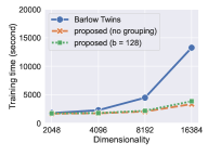
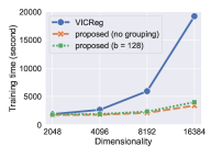
Peak GPU allocated memory

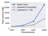
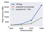
Figure 2: Training time and memory usage on ImageNet-100 with ResNet-18 on a single GPU.

Dimensionality of embeddings and computational cost.

Fig. 2 presents the elapsed time and the peak GPU memory allocation over 10 epochs on ImageNet-100 on a single GPU, with varying dimensionality of the projected embeddings: $d\in\{2048,\allowbreak 4096,\allowbreak 8192,16384\}$. The improvement over Barlow Twins and VICReg becomes noticeable as $d$ is increased; at $d=8192$, the proposed models (without grouping) are 2.8 times as fast as VICReg, and 2.2 times as fast as Barlow Twins; while at $d=16384$, they are 5.7 times as fast as VICReg, and 4.0 times as fast as Barlow Twins. For both $d=8192$ and $16384$, memory consumption is reduced by more than half. See Secs. E.2 and E.4 for the results with the ResNet-50 backbone on multiple GPUs and the detail of forward/backward/loss computation time.

Table 5: The effect of feature permutation: accuracy (%) and training time per 10 epochs (second) on ImageNet-100.

Grouping	Permutation	Top-1	Top-5	Time
no	no	59.64	85.20	1646.2
	yes	79.94	94.76	1668.7
$b=128$	no	73.58	93.36	1697.5
	yes	81.02	95.24	1709.6

(a)

Grouping	Permutation	Top-1	Top-5	Time
no	no	57.42	84.26	1692.2
	yes	79.20	94.96	1718.0
$b=128$	no	66.26	89.68	1802.1
	yes	80.04	94.98	1813.3

(b)

Effectiveness of feature permutation.

Tab. 5 presents the effect of feature permutation on ImageNet-100 at $d=2048$. Regardless of whether grouping is used, the accuracy decreases significantly without permutation, suggesting that feature permutation is essential for the effectiveness of our proposed regularizer. As illustrated in the column “Time” in Tab. 5, the cost of permutation is negligible, even though it was performed as frequently as every batch iteration.

Table 6: The regularizers of Barlow Twins and VICReg applied to the embeddings produced by the proposed models. Perm.: permutation; Diff: difference to the baselines.

			Normalized Barlow
Model	Grouping	Perm.	Twins loss (Eq. 16)	Diff
Barlow Twins	—	—	0.005	0
Proposed	no	no	0.564	0.559
		yes	0.010	0.005
	$b=128$	no	0.049	0.044
		yes	0.009	0.004

(c)

			Normalized
Model	Grouping	Perm.	VICReg loss (Eq. 17)	Diff
VICReg	—	—	0.002	0
Proposed	no	no	1.999	1.997
		yes	0.011	0.009
	$b=128$	no	0.379	0.377
		yes	0.007	0.005

(d)

We also quantitatively evaluate the degree of decorrelation obtained by feature permutation. After the proposed models are trained, we compute the normalized values of Barlow Twins’ and VICReg’s regularizers applied to the embeddings $A,B$ output by the proposed models, given as follows:

$$\frac{R_{\textup{off}}(\mathbf{C}(\mathrm{A},\mathrm{B}))}{d(d-1)}$$ (16)

$$\frac{R_{\textup{off}}(\mathbf{K}(\mathrm{A}))+R_{\textup{off}}(\mathbf{K}(\mathrm{B}))}{2d(d-1)}$$ (17)

The normalization factor $d(d-1)$ is to make the resulting values the means over $d(d-1)$ off-diagonal elements of $\mathbf{K}(\mathrm{A})$, $\mathbf{K}(\mathrm{B})$, and $\mathbf{C}(\mathrm{A},\mathrm{B})$. Since VICReg has regularization terms for $\mathbf{K}(\mathrm{A})$ and $\mathbf{K}(\mathrm{B})$, its loss is further divided by 2. Tab. 6 presents the results on ImageNet-100 ($d$=2048). We observe that feature permutation promotes decorrelation from the point of view of the baseline loss functions.

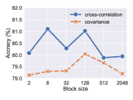
(a)

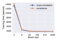
(b)

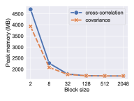
(c)

Figure 3: The impact of the block size on ImageNet-100. The $x$-axis indicates the block size $b$.

Impact of block size in feature grouping.

To evaluate the effect of feature grouping on ImageNet-100, we fix the embedding dimension at $d=2048$ and change the block size $b\in\{2,4,8,...,2048\}$. The block size $b=d=2048$ corresponds to no feature grouping. Figure 3 presents the result, which indicates that unless $b$ is extremely small (i.e., 8 or less), there is no significant increase in training time or GPU memory usage. Setting $b$ to a moderate size, such as $b=128$, improves performance.

6 Conclusion

We have proposed a new decorrelating regularizer for non-contrastive SSL. Given $d$-dimensional embeddings of $n$ samples, the regularizer can be computed in $O(nd\log d)$ time, which is an improvement over the $O(nd^{2})$ time required by the existing models (Barlow Twins and VICReg). The reduced memory consumption allows for a larger batch size, which in general enables more effective models to be learned. We also proposed a feature permutation technique to alleviate the weakness of our regularizer.

With our regularizer, the speed-up is most notable with networks with a lightweight backbone, wherein computation at the loss node takes a large part of training time. This makes our method an attractive option to use with knowledge-distilled backbones [18, 13].

The proposed method is not limited to SSL but potentially useful to a wider range of applications that involve decorrelation. We plan to pursue this avenue in future work.

Appendix A Derivation of Eq. 8

Let $d$-dimensional vectors $\mathbf{x}=[x_{0}\cdots x_{d-1}]^{\textup{T}}$, $\mathbf{y}=[y_{0}\cdots y_{d-1}]^{\textup{T}}$. We first show $\mathop{\textup{inv}}(\mathbf{x})*\mathbf{y}=\sum_{j=0}^{d-1}x_{j}y_{(i+j)\bmod d}$.

$$\left[\mathop{\textup{inv}}(\mathbf{x})*\mathbf{y}\right]_{i} =\sum_{j=0}^{d-1}[\mathop{\textup{inv}}(\mathbf{x})]_{j}\,y_{(i-j)\bmod d}$$

$$=\sum_{j=0}^{d-1}x_{(d-j)\bmod d}\;y_{(i-j)\bmod d} \because\;[\mathop{\textup{inv}}(\mathbf{x})]_{j}=x_{(d-j)\bmod d}$$

$$=\sum_{j^{\prime}=0}^{d-1}x_{j^{\prime}}\,y_{(i-(d-j^{\prime}))\bmod d} \because\;\text{substituting }j^{\prime}=(d-j)\bmod d$$

$$=\sum_{j^{\prime}=0}^{d-1}x_{j^{\prime}}\,y_{(i+j^{\prime})\bmod d} \because\;(a-d)\bmod d=a\bmod d$$

$$=\sum_{j=0}^{d-1}\left[\mathbf{x}{\mathbf{y}}^{\textup{T}}\right]_{j,(i+j)\bmod d}. \because\;\text{renaming variable }j^{\prime}\to j$$

Setting $\mathbf{x}=\mathbf{a}^{(k)}$ and $\mathbf{y}=\mathbf{b}^{(k)}$, we obtain Eq. 8 in Sec. 4.2. In the literature (e.g., [22, 25]), $\mathop{\textup{inv}}(\mathbf{x})*\mathbf{y}$ is called the circular correlation of $\mathbf{x}$ and $\mathbf{y}$, and the above equation is usually presented as its definition.

Appendix B Regularizers Based on Sums of Feature Covariances

As mentioned in Sec. 4.5, if we substitute $R_{\textup{sum}}$ for $R_{\textup{off}}$ in the loss function of VICReg given in Eq. 3, we obtain regularization based on the covariance matrices $\mathbf{K}(\mathrm{A}),\mathbf{K}(\mathrm{B})$ of individual views. The resulting regularizer for $\mathbf{K}(\mathrm{A})$ is:

$$R_{\textup{sum}}(\mathbf{K}(\mathrm{A})) =\sum_{i=1}^{d-1}\|[\mathop{\textup{sumvec}}(\mathbf{K}(\mathrm{A}))]_{i}\|_{q}^{q},$$ (18)

where hyperparameter $q\in\{1,2\}$. The regularizer for $\mathbf{K}(\mathrm{B})$ has the same form and is omitted.

$R_{\textup{sum}}(\mathbf{K}(\mathrm{A}))$ can be efficiently computed by FFT, in a similar manner to $R_{\textup{sum}}(\mathbf{C}(\mathrm{A},\mathrm{B}))$. For brevity, assume that set $\mathrm{A}$ is centered; i.e., all features have mean $0$ in $\mathrm{A}$. In this case, its covariance matrix is $\mathbf{K}(\mathrm{A})=(1/(n-1))\sum_{k=1}^{n}\mathbf{a}^{(k)}{\mathbf{a}^{(k)}}^{\textup{T}}$.

Noting that $\mathop{\mathscr{F}}(\mathop{\textup{inv}}(\mathbf{a}^{(k)})=\overline{\mathop{\mathscr{F}}(\mathbf{a}^{(k)})}$ and the convolution theorem $\mathop{\mathscr{F}}(\mathbf{x}*\mathbf{y})=\mathop{\mathscr{F}}(\mathbf{x})\circ\mathop{\mathscr{F}}(\mathbf{y})$, we have

$$\mathop{\textup{sumvec}}(\mathbf{K}(\mathrm{A})) =\frac{1}{n-1}\sum_{k=1}^{n}\mathop{\textup{inv}}(\mathbf{a}^{(k)})*\mathbf{a}^{(k)}$$

$$=\frac{1}{n-1}\sum_{k=1}^{n}\overbrace{\mathop{\mathscr{F}^{-1}\!}\left(\overline{\mathop{\mathscr{F}}(\mathbf{a}^{(k)})}\circ\mathop{\mathscr{F}}(\mathbf{a}^{(k)})\right)}^{\mathop{\textup{inv}}(\mathbf{a}^{(k)})*\mathbf{a}^{(k)}}$$

$$=\frac{1}{n-1}\mathop{\mathscr{F}^{-1}\!}\left(\sum_{k=1}^{n}\overline{\mathop{\mathscr{F}}(\mathbf{a}^{(k)})}\circ\mathop{\mathscr{F}}(\mathbf{a}^{(k)})\right),$$ (19)

The grouping version is also straightforward. Partitioning $\mathbf{K}(\mathrm{A})$ into block submatrices of size $b\times b$, i.e., $\mathbf{K}(A)=[\mathbf{K}_{ij}]$ ($i,j=1,\ldots,\lceil d/b\rceil$), where $\mathbf{K}_{ij}\in\mathbb{R}^{b\times b}$, and applying $R_{\textup{sum}}^{(b)}$ defined in Eq. 13 to it, we obtain

$$R_{\textup{sum}}^{(b)}(\mathbf{K}(\mathrm{A})) =\sum_{i=1}^{\lceil d/b\rceil}\sum_{\ell=1}^{b-1}\|[\mathop{\textup{sumvec}}(\mathbf{K}_{ii})]_{\ell}\|_{q}^{q}+\sum_{\begin{subarray}{c}i,j=1\\ i\neq j\end{subarray}}^{\lceil d/b\rceil}\sum_{\ell=0}^{b-1}\left\|[\mathop{\textup{sumvec}}(\mathbf{K}_{ij})]_{\ell}\right\|_{q}^{q}.$$ (20)

where block size $b$ is the hyperparameter that controls the granularity of the summary computation. When $q=2$ and $b=d$, i.e., the block size is $(b/d)\times(b/d)=1\times 1$, the regularizer $R_{\textup{sum}}^{(b)}(\mathbf{K}(\mathrm{A}))$ reduces to $R_{\textup{off}}(\mathbf{K}(\mathrm{A}))$ of VICReg.

Appendix C Summary of Computational Complexity

Table 7: Complexity of loss computation. The space complexity includes $O(nd)$ memory needed to store input embeddings. Grouping = $b$ indicates $b$ being the size of the group (i.e., block size).

Regularizer	Grouping	Time	Space
Barlow Twins	—	$O(nd^{2})$	$O(nd+d^{2})$
VICReg	—	$O(nd^{2})$	$O(nd+d^{2})$
Proposed ($R_{\textup{sum}}$)	no	$O(nd\log d)$	$O(nd)$
Proposed ($R_{\textup{sum}}^{(b)}$)	$b$	$O((nd^{2}/b)\log b)$	$O(nd)$

Tab. 7 summarizes the computational complexity of the regularizers discussed in this paper. As the table shows, the proposed regularizers are faster and cheaper than the Barlow Twins and VICReg in terms of time and space complexity.

Appendix D Detailed Experimental Setups

All the experiments in Sec. 5 were conducted on commercial Linux servers with CUDA v11.6.2 and cuDNN v8. We implemented our model using PyTorch v1.12.0 [21] and solo-learn v1.0.5 [28], a library of self-supervised methods for visual representation learning built on top of PyTorch and PyTorch Lightning v1.6.4. We also used NVIDIA DALI, a library for data loading and pre-processing to accelerate deep learning applications. For object detection, detectron2 [31] was used. To manage the experiments, we used Weights & Biases, a machine learning platform for the tracking and visualization of experiments [2]. As PyTorch v1.12.0 only provides experimental support for half precision FFT, we trained every model with 32-bit precision, including Barlow Twins and VICReg.

D.1 Compared Methods

Table 8: Loss functions and regularizers in the proposed method (with and without grouping), Barlow Twins, and VICReg. Grouping = $b$ indicates $b$ being the size of the group (i.e., block size).

Method	Grouping	Regularizer function $R$
Barlow Twins	—	$R_{\textup{off}}$
Proposed	no	$R_{\textup{sum}}$
Proposed	$b$	$R_{\textup{sum}}^{(b)}$

(d) Cross-correlation–regularization with Barlow Twins–style loss function $L=\sum_{i}\left(1-[\mathbf{C}(\mathrm{A},\mathrm{B})]_{ii}\right)^{2}+\lambda R(\mathbf{C}(\mathrm{A},\mathrm{B}))$

Method	Grouping	Regularizer function $R$
VICReg	—	$R_{\textup{off}}$
Proposed	no	$R_{\textup{sum}}$
Proposed	$b$	$R_{\textup{sum}}^{(b)}$

(e) Covariance regularization with VICReg-style loss function $L=\frac{\alpha}{n}\sum_{i}\|\mathbf{a}^{(i)}-\mathbf{b}^{(i)}\|^{2}_{2}+\frac{\mu}{d}\left(R_{\textup{var}}(\mathbf{K}(\mathrm{A}))+R_{\textup{var}}(\mathbf{K}(\mathrm{B}))\right)+\frac{\nu}{d}\left(R(\mathbf{K}(\mathrm{A}))+R(\mathbf{K}(\mathrm{B}))\right)$

In each comparison, the proposed method and the two baselines, Barlow Twins and VICReg, used an identical network architecture, with the exception of the training loss. The loss functions of the baselines are given by Eqs. 1 and 3, which are repeated below as Eqs. 21 and 22 for convenience. Let $\mathrm{A}=\{\mathbf{a}^{(i)}\}_{i=1}^{m}$, $\mathrm{B}=\{\mathbf{b}^{(i)}\}_{i=1}^{m}$ be the embeddings of the two views, with $i=1,\ldots,m$ indicating the original sample indices, $\mathbf{K}(\mathrm{A}),\mathbf{K}(\mathrm{B})\in\mathbb{R}^{d\times d}$ be their respective covariance matrices, and $\mathbf{C}(\mathrm{A},\mathrm{B})\in\mathbb{R}^{d\times d}$ be the cross-correlation matrices between $A$ and $B$.

$$L_{\textup{BT}} =\sum_{i=0}^{d-1}\left(1-[\mathbf{C}(\mathrm{A},\mathrm{B})]_{ii}\right)^{2}+\lambda R_{\textup{off}}(\mathbf{C}(\mathrm{A},\mathrm{B})),$$ (21)

$$L_{\textup{VIC}} =\frac{\alpha}{n}\sum_{i=1}^{m}\|\mathbf{a}^{(i)}-\mathbf{b}^{(i)}\|^{2}_{2}+\frac{\mu}{d}\left(R_{\textup{var}}(\mathbf{K}(\mathrm{A}))+R_{\textup{var}}(\mathbf{K}(\mathrm{B}))\right)+\frac{\nu}{d}\left(R_{\textup{off}}(\mathbf{K}(\mathrm{A}))+R_{\textup{off}}(\mathbf{K}(\mathrm{B}))\right),$$ (22)

where hyperparameters $\alpha,\mu,\nu,\lambda\geq 0$ determine the importance of individual terms, and the regularization functions are given by

$$R_{\textup{off}}(\mathbf{M}) =\sum_{i=0}^{d-1}\sum_{\begin{subarray}{c}j=0\\ j\neq i\end{subarray}}^{d-1}[\mathbf{M}]_{ij}^{2},$$

$$R_{\textup{var}}(\mathbf{M}) =\sum_{i=0}^{d-1}\text{max}(0,\gamma-\sqrt{[\mathbf{M}]_{ii}}).$$

For the proposed method, we replace all occurrences of $R_{\textup{off}}$ in Eqs. 21 and 22 with either $R_{\textup{sum}}$ (Eq. 6) or $R_{\textup{sum}}^{(b)}$ (Eq. 13) depending on whether grouping is used. These functions are repeated below.

$$R_{\textup{sum}}(\mathbf{M}) =\sum_{i=1}^{d-1}\|[\mathop{\textup{sumvec}}(\mathbf{M})]_{i}\|_{q}^{q},$$ (23)

$$R_{\textup{sum}}^{(b)}(\mathbf{M}) =\sum_{i=1}^{\lceil d/b\rceil}\sum_{\ell=1}^{b-1}\|[\mathop{\textup{sumvec}}(\mathbf{M}_{ii})]_{\ell}\|_{q}^{q}+\sum_{\begin{subarray}{c}i,j=1\\ i\neq j\end{subarray}}^{\lceil d/b\rceil}\sum_{\ell=0}^{b-1}\|[\mathop{\textup{sumvec}}(\mathbf{M}_{ij})]_{\ell}\|_{q}^{q},$$ (24)

where $\mathbf{M}=[\mathbf{M}_{ij}]$ is a block matrix with block elements $\mathbf{M}_{ij}\in\mathbb{R}^{b\times b}$, $i,j=1,\ldots,\lceil d/b\rceil$.

Tab. 8 summarizes the regularizers and loss functions for Barlow Twins, VICReg, and the proposed models.

D.2 Data Augmentation

Following the Barlow Twins paper [33], we used non-symmetric parameters for Barlow Twins-style objectives. For VICReg-style objectives in ImageNet-100 experiments, we used the symmetrized augmentation pipeline reported in the VICReg paper [1, Appendix C.1]. Following a comment in the VICReg GitHub repository, we used the non-symmetric augmentation parameters (the same parameters as in Barlow Twins) for ImageNet experiments.

D.3 Hyperparameters

ImageNet-100.

For ImageNet-100 experiments, we followed the optimization procedure described in [28]. To train models, stochastic gradient descent (SGD) was used with the LARS optimizer [32] for 400 epochs. We used linear warm-up with cosine annealing decay for the learning rate scheduler. The batch size was wet to 256 (per GPU batch size is 32). The loss scaling value and the importance coefficients for the proposed regularizers ($\nu$ in Eq. 3 and $\lambda$ in Eq. 1) were sought by grid search. In addition to these parameters, we further tuned the block size and $q$ in our regularizers (Eqs. 6 and 13).

In linear evaluation, linear classifiers was optimized with SGD for 100 epochs. In training for ImageNet-100, we used the hyperparameters provided by the solo-learn library.

Tab. 9 summarizes the hyperparameters for ImageNet-100 experiments.

Table 9: The hyperparameters for ImageNet-100 experiments that were used for training models. The hyperparameters for Barlow Twins and VICReg were set to the values reported by [28]. For the proposed methods, we found values by grid search.

Method	Grouping	Loss scale	$q$	$\lambda$
Barlow Twins	—	0.1	—	0.0051
Proposed (Barlow Twins–style)	no	0.125	2	$2^{-10}$
Proposed (Barlow Twins–style)	$b=128$	0.125	2	$2^{-10}$

(f) Cross-correlation regularization with Barlow Twins–style loss function

Method	Grouping	Loss scale	$q$	$\nu$
VICReg	—	—	—	1.0
Proposed (VICReg-style)	no	0.25	1	1.0
Proposed (VICReg-style)	$b=128$	0.25	1	2.0

(g) Covariance regularization

Learning rate	Weight decay	Batch size	Warmup epochs	$\alpha$	$\mu$
0.3	$10^{-4}$	256	10	25.0	25.0

(h) All other hyperparameters were set to the values reported by [28].

Pretrained model	Learning rate	Steps for learning rate decay	Weight decay	Batch size
Barlow Twins / Proposed (Barlow Twins–style)	0.1	[60, 80]	0	256
VICReg / Proposed (VICReg-style)	0.3	[60, 80]	0	512

(i) Hyperparameters for linear evaluation on ImageNet-100.

ImageNet.

For ImageNet experiments, we followed the optimization procedure described in [33, 1]. We used SGD with the LARS optimizer for 1000 epochs and linear warmup with cosine annealing decay. We set the batch size to 1024 (per GPU batch size is 128) and used a learning rate of 0.25 by reference to the Barlow Twins GitHub repository. We searched for $\lambda$ and $q$ for the proposed regularizers by grid search.

In the linear evaluation on ImageNet, the linear head was trained for 100 epochs with SGD and cosine learning rate decay. We tuned the learning rate and batch size for the proposed methods. For Barlow Twins and VICReg, the learning rate and batch size are set to the values reported in the original papers [33, 1].

In object detection, we trained a Faster R-CNN with a C-4 backbone for 24K iterations. The backbone is initialized with the pretrained ResNet-50 backbone. Following [16, 33, 1], we set the batch size to 16 (per GPU batch size is 2) and used a step learning rate decay (divided by 10 at 18K and 22K iterations) with a linear warmup (slope of 0.333 for 1K iterations). We tuned the learning rate and the region proposal network loss weight for the proposed methods.

Tab. 10 summarizes the hyperparameters for ImageNet experiments.

Table 10: The hyperparameters for ImageNet experiments that were used for training models.

Method	Grouping	Loss scale	$q$	$\lambda$
Barlow Twins	—	0.024	—	0.0051
Proposed (Barlow Twins–style)	no	0.024	2	$2^{-11}$
Proposed (Barlow Twins–style)	$b=128$	0.024	2	$2^{-11}$

(j) Cross-correlation regularization

Method	Grouping	Loss scale	$q$	$\alpha$	$\mu$	$\nu$
VICReg	—	—	—	25.0	25.0	1.0
Proposed (VICReg-style)	no	—	1	2.5	2.5	0.1

(k) Covariance regularization

Learning rate	Weight decay	Batch size	Warmup epochs
0.25	$10^{-6}$	1024	10

(l) Hyperparameters for optimization.

Pretrained model	Learning rate	Learning rate decay	Weight decay	Batch size
Barlow Twins	0.3	cosine decay	$10^{-6}$	256
VICReg	0.02	cosine decay	$10^{-6}$	256
Proposed (Barlow Twins–style)	0.125	cosine decay	$10^{-6}$	2048
Proposed (VICReg-style)	0.125	cosine decay	$10^{-6}$	256

(m) Hyperparameters for linear evaluation on ImageNet.

Pretrained model	Learning rate	Region proposal network loss weigh
Proposed (Barlow Twins–style)	0.125	0.03125
Proposed (VICReg-style)	0.125	0.125

(n) Hyperparameters for object detection on VOC07+12.

D.4 Evaluation of Training Time and Memory Consumption

To discuss empirical complexity, we measured the elapsed time and peak GPU memory allocation over ten epochs. We conducted three trials and reported the average time and memory allocation. To avoid communication overhead between GPUs, we evaluated the results of single GPU training (not distributed data parallel training) unless otherwise noted. The batch size was set to 32 for ImageNet-100 and 128 for ImageNet as in pretraining settings (per GPU batch size is 32 and 128). The number of workers (the argument “num_workers” in the solo-learn library used for implementation) is set to 32 for ImageNet-100 and 4 for ImageNet.

We used the Simple Profiler in PyTorch Lightning to measure training time. From the profiler output, the value of the “Total time (s)” in the “run_training_epoch” line was extracted and plotted as the training time in Figs. 3, 7, 2, 4, 5, 6 and 6. We used a function in PyTorch to monitor memory occupied by tensors. The value of “Peak Usage” in the “Allocated memory” line was used as the peak GPU memory allocation.

As regards the total training time in Tab. 4, we reported the runtime counted by WandB. As mentioned in the footnote of Sec. 5.2, our experiment was performed on a commercial cloud platform that terminates a session after three days. To finish training Barlow Twins and VICReg with 8 GPUs for 1000 epochs on ImageNet, we needed three sessions, and the proposed model only two (see Tab. 4). The timing reported in Tab. 4 is the run time of these sessions that includes the time for initialization at the beginning of each session. This initialization takes only 3–5 seconds at each session and does not affect the trend observed in the table. Note that in addition to this initialization, data copy takes about 15 minutes at the start of a session, but this has already been excluded from the timing in Tab. 4.

D.5 Computational Resources

We used a cloud computing platform for the experiments. In the main experiments, we trained models with eight Nvidia A100-SXM4 GPUs on this platform. We used a single Nvidia A100 GPU to evaluate empirical complexity, except where noted.

D.6 License of the Assets

PyTorch has a BSD-style license. Solo-learn has an MIT license. PyTorch Lightning is licensed under the Apache License 2.0. The ImageNet dataset is publicly available and frequently used as the benchmark dataset. The category list of ImageNet-100 is also publicly available.

Appendix E Additional Experiments

E.1 Impact of Hyperparameter $q$

Table 11: The accuracy with $q\in\{1,2\}$ on ImageNet-100.

Model	Grouping	$q$	Top-1	Top-5
Proposed (Barlow Twins–style)	no	1	75.94	94.28
		2	79.94	94.76
	$b=128$	1	76.44	94.46
		2	81.02	95.24
Proposed (VICReg-style)	no	1	79.20	94.96
		2	57.98	84.56
	$b=128$	1	80.04	94.98
		2	71.78	92.54

We investigate the effect of the hyperparameter $q$ in our regularizers (Eqs. 6 and 13). Tab. 11 shows the results with $q\in\{1,2\}$ on ImageNet-100 ($d=2048$). The results indicate that $q=1$ works better than $q=2$ in VICReg-style covariance regularizers. Conversely, $q=2$ works well in Barlow Twins–style cross-correlation regularizers.

E.2 Training Time with ResNet-50 Backbone

	Cross-correlation regularization	Covariance regularization
Elapsed time per 10 epochs
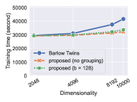
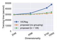
Peak GPU allocated memory

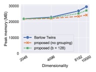
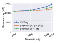
Figure 4: Training time and memory usage on ImageNet with ResNet-50 on a single GPU.

Figure 4 presents the single GPU training cost with ResNet-50 on ImageNet. Due to GPU memory limitation, we were unable to run Barlow Twins and VICReg at $d=16384$, and also the grouped version of the proposed models with block size $b=128$. Instead of $d=16384$, we present the results at $d=10000$. As in the results of ImageNet-100, we can observe that the proposed regularizers are more efficient than the existing regularizers. At $d=8192$, the proposed model (without grouping) is 1.3 ($=41414.3/31280.0$) times faster than VICReg, and 1.2 ($=37522.0/31306.0$) times faster than Barlow Twins; while at $d=10000$, it is 1.5 ($=47448.0/32208.3$) times faster than VICReg, and 1.3 times ($=41546.3/32143.7$) faster than Barlow Twins.

E.3 Training Time with Distributed Data Parallel

	Cross-correlation regularization family	Covariance regularization family
Elapsed time per 10 epochs

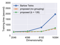
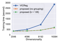
Figure 5: The elapsed DDP training time on ImageNet-100 with ResNet-18.

Except for Tab. 4, the training time figures reported in Sec. 5 and Sec. E.2 were measured on a single GPU. Here we evaluate the timing of distributed data parallel (DDP) training, when multiple GPUs are available. Fig. 5 shows the elapsed time of DDP training for ten epochs on eight A100 GPUs. With DDP, the cost of communication between GPUs emerges as an additional factor determining the total computational time, and hence the relative merit of our method in reducing loss computation time is expected to diminish. Although this is certainly true, our method is still effective, improving the computation time by a factor of more than 2.2 ($=945.5/428.7$) for VICReg and 2.0 ($=740.6/366.4$) for Barlow Twins when $d=8192$ and a factor of 4.4 ($=2833.3/647.1$) and 3.1 ($=1943.7/622.7$) when $d=16384$.

	Cross-correlation regularization family	Covariance regularization family
Elapsed time per 10 epochs

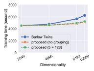
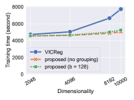
Figure 6: The elapsed DDP training time on ImageNet with ResNet-50.

Fig. 6 shows the elapsed time on ImageNet with ResNet-50. As in ImageNet-100 with ResNet-18 (Fig. 5), our method improves speed, but the speed-up factor is smaller: 1.4 ($=6658.1/4858.9$) for VICReg and 1.2 ($=5657.6/4868.7$) for Barlow Twins when $d=8192$. When $d=10000$, the factors are 1.5 ($=7729.9/5035.1$) for VICReg and 1.2 ($=6247.7/5129.6$) for Barlow Twins.

	Cross-correlation regularization family	Covariance regularization family
Elapsed time per 10 epochs

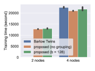
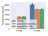
Figure 7: The elapsed multi-node DDP training time on ImageNet with ResNet-50 ($d=16384$).

In the ImageNet experiments (Figs. 4 and 6), all models triggered an out-of-GPU-memory error when $d=16384$. We thus use multi-node DDP training for $d=16384$. We evaluated two situations: training using 2 nodes and 4 nodes. In both situations, we set the effective batch size to 1024. Figure 7 shows the results. Barlow Twins and VICReg still ran out of memory under 2 nodes, but the proposed models (with or without grouping) worked in this situation thanks to their efficient memory usage. With 4 nodes, all models were trained successfully, and the proposed models were slightly faster than Barlow Twins and VICReg. However, in this setting, there is no point in training our models using 4 nodes, when they are trainable on 2 nodes. If we compare the speed of our models trained on 2 nodes with Barlow Twins and VICReg (which failed to be trained on 2 nodes) on 4 nodes, the advantage of our models becomes more pronounced.

E.4 Computation Time for Forward and Backward Passes

We analyzed the training time spent for the forward pass (in the model network excluding the loss node), forward loss computation, and backpropagation. These three types are denoted by “Forward (model)”, “Forward (loss)”, and “Backward (model + loss)”, respectively. These measurements were quoted from the “Total time (s)” column in the respective lines in the output of the Simple Profiler in PyTorch Lightning. Note that by default, the profiler only reports total forward computation time. To separate the total time into “Forward (model)” and “Forward (loss)”, we specified custom measurement points in our code where the model (backbone network and projection network) forward computation and the loss computation are performed. Since the custom measurement points did not work for backpropagation, we plot the value of “Strategy.backward” line as the total backpropagation time “Backward (model + loss)”.

Fig. 8 presents the results. The times for loss computation and backpropagation both improved with our method; see Tabs. 12 and 13 for the detail of improvements. The improvement in backpropagation is due to reduced time at the loss node, because Barlow Twins and the proposed method have the same model network and differ only in the loss used. This reduction in the backpropagation time is not surprising because the same computation graph is traversed in both the forward and backward passes, and therefore their asymptotic computational complexity is roughly identical.

Setting	Cross-correlation regularization	Covariance regularization
(a) ImageNet-100 ResNet-18 1 GPU
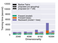
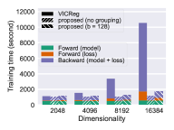
(b) ImageNet ResNet-50 1 GPU
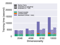
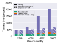
(c) ImageNet-100 ResNet-18 8-GPU DDP
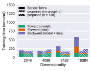
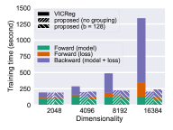
(d) ImageNet ResNet-50 8-GPU DDP

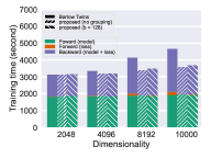
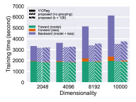
Figure 8: The elapsed 10-epoch training time spent on forward model (green) and loss (orange) computation, and backpropagation (total of model and loss; purple).

Table 12: The improvements for loss and backward computations on ImageNet100 with ResNet-18.

Model	#GPU	$d$	Forward (loss)	Backward (model + loss)
Barlow Twins–style	1	8192	7.5 ($=285.5/38.0$)	2.5 ($=1101.6/448.6$)
		16384	23.1 ($=1038.7/44.9$)	6.3 ($=2959.1/468.0$)
	8	8192	7.4 ($=52.5/7.1$)	1.9 ($=124.3/67.1$)
		16384	24.8 ($=183.6/7.4$)	3.9 ($=274.0/70.3$)
VICReg-style	1	8192	6.0 ($=323.0/53.5$)	5.4 ($=2548.8/473.2$)
		16384	19.5 ($=1166.5/59.8$)	18.3 ($=8820.3/482.0$)
	8	8192	7.0 ($=62.6/8.9$)	4.1 ($=300.5/74.2$)
		16384	24.2 ($=215.7/8.9$)	13.2 ($=996.3/75.5$)

Table 13: The improvements for loss and backward computations on ImageNet with ResNet-50.

Model	#GPU	$d$	Forward (loss)	Backward (model + loss)
Barlow Twins–style	1	8192	9.5 ($=751.1/79.2$)	2.9 ($=8594.0/2977.5$)
		10000	13.2 ($=1097.5/83.2$)	3.6 ($=11583.0/3181.2$)
	8	8192	10.6 ($=125.8/11.9$)	1.5 ($=2129.1/1463.5$)
		10000	15.0 ($=184.4/12.3$)	1.6 ($=2552.2/1593.5$)
VICReg-style	1	8192	8.4 ($=898.8/107.0$)	4.1 ($=12346.0/3016.6$)
		10000	11.9 ($=1311.1/110.3$)	5.4 ($=17249.3/3221.7$)
	8	8192	18.1 ($=280.7/15.5$)	2.0 ($=2937.3/1467.1$)
		10000	25.2 ($=415.7/16.5$)	2.4 ($=3752.4/1557.9$)

Appendix F Code

LABEL:lst:covsum and LABEL:lst:xcorr present Python-based implementations for covariance and cross-correlation regularizers (without feature grouping). As explained in Sec. 4, the summary vectors can be efficiently calculated with FFT (see Listing LABEL:lst:sumvec).

In the computation of the proposed regularizers, we do not conduct collective operations, such as all-reduce and gather functions.

⬇

1# Z1, Z2: projected image embeddings (n x d)

2# q: a hyperprameter for L_q^q norm

3

4def xsum_regularizer(Z1, Z2, G, q):

5 # pre-process: centering and normalization

6 Z1 = batch_normalization(Z1)

7 Z2 = batch_normalization(Z2)

8

9 # feature permutation

10 idx = torch.randperm(Z1.shape[1])

11 Z1 = Z1[:, idx]

12 Z2 = Z2[:, idx]

13

14 # summary vector

15 sumvec = cal_sumvec(Z1, Z2, 0) / n

16

17 # loss for off-diagonal elements

18 if q == 1:

19 loss = torch.sum(sumvec[1:].abs())

20 elif q == 2:

21 loss = torch.sum(sumvec[1:].pow(2))

22

23 return loss

Listing 1: Computing Barlow Twins–style cross-correlation regularizer

⬇

1# Z: projected image embeddings ([n: batch size] x [d: embedding dimension])

2# q: a hyperparameter for L_q^q norm

3

4def covsum_regularizer(Z, blck_size, q):

5 # pre-process: centering

6 Z = Z - Z.mean(dim=0)

7

8 # feature permutation

9 idx = torch.randperm(Z.shape[1])

10 Z = Z[:, idx]

11

12 # summary vector

13 sumvec = cal_sumvec(Z, Z, 0) / (n - 1)

14

15 # loss for off-diagonal elements

16 if q == 1:

17 loss = torch.sum(sumvec[1:].abs())

18 elif q == 2:

19 loss = torch.sum(sumvec[1:].pow(2))

20

21 return loss

Listing 2: Computing VICReg-style covariance regularizer

⬇

1def cal_sumvec(z1, z2, dim):

2 fz1 = fft.rfft(z1)

3 fz2 = fft.rfft(z2)

4 fz1_conj = fz1.conj()

5 fz_prod = fz1_conj * fz2

6 fc = fz_prod.sum(dim=dim)

7 sumvec= fft.irfft(fc)

8 return sumvec

Listing 3: Summary vector computation

References

- [1] Adrien Bardes, Jean Ponce, and Yann LeCun. VICReg: Variance-invariance-covariance regularization for self-supervised learning. In ICLR, 2022.
- [2] Lukas Biewald. Experiment tracking with Weights and Biases. Software available from https://www.wandb.com/, 2020.
- [3] A. Borsellino and T. Poggio. Convolution and correlation algebras. Kybernetik, 13(2):113–122, 1973.
- [4] Ting Chen, Simon Kornblith, Mohammad Norouzi, and Geoffrey Hinton. A simple framework for contrastive learning of visual representations. In ICML, pages 1597–1607, 2020.
- [5] Ting Chen, Simon Kornblith, Kevin Swersky, Mohammad Norouzi, and Geoffrey E. Hinton. Big self-supervised models are strong semi-supervised learners. In NeurIPS, pages 22243–22255, 2020.
- [6] Xinlei Chen and Kaiming He. Exploring simple Siamese representation learning. In CVPR, pages 15750–15758, 2021.
- [7] Xinlei Chen, Saining Xie, and Kaiming He. An empirical study of training self-supervised vision transformers. In ICCV, pages 9640–9649, 2021.
- [8] James W. Cooley and John W. Tukey. An algorithm for the machine calculation of complex Fourier series. Mathematics of Computation, 19(90):297–301, 1965.
- [9] Jia Deng, Wei Dong, Richard Socher, Li-Jia Li, Kai Li, and Li Fei-Fei. ImageNet: A large-scale hierarchical image database. In CVPR, pages 248–255, 2009.
- [10] Debidatta Dwibedi, Yusuf Aytar, Jonathan Tompson, Pierre Sermanet, and Andrew Zisserman. With a little help from my friends: Nearest-neighbor contrastive learning of visual representations. In ICCV, pages 9588–9597, 2021.
- [11] Aleksandr Ermolov, Aliaksandr Siarohin, Enver Sangineto, and Nicu Sebe. Whitening for self-supervised representation learning. In ICML, pages 3015–3024, 2021.
- [12] Mark Everingham, Luc Van Gool, Christopher KI Williams, John Winn, and Andrew Zisserman. The PASCAL visual object classes (VOC) challenge. International Journal of Computer Vision, 88(2):303–338, 2010.
- [13] Yuting Gao, Jia Xin Zhuang, Shaohui Lin, Hao Cheng, Xing Sun, Ke Li, and Chunhua Shen. DisCo: Remedying self-supervised learning on lightweight models with distilled contrastive learning. In ECCV, pages 237–253, 2022.
- [14] Jean-bastien Grill, Florian Strub, Florent Altché, Corentin Tallec, Pierre H Richemond, Elena Buchatskaya, Carl Doersch, Bernardo Avila Pires, Zhaohan Daniel Guo, Mohammad Gheshlaghi Azar, Bilal Piot, Koray Kavukcuoglu, Rémi Munos, and Michal Valko. Bootstrap your own latent: A new approach to self-supervised learning. In NeurIPS, pages 21271–21284, 2020.
- [15] Katsuhiko Hayashi and Masashi Shimbo. On the equivalence of holographic and complex embeddings for link prediction. In ACL ’17, pages 554–559, 2017.
- [16] Kaiming He, Haoqi Fan, Yuxin Wu, Saining Xie, and Ross Girshick. Momentum contrast for unsupervised visual representation learning. In CVPR, pages 9729–9738, 2020.
- [17] Kaiming He, Xiangyu Zhang, Shaoqing Ren, and Jian Sun. Deep residual learning for image recognition. In CVPR, pages 770–778, 2016.
- [18] Geoffrey Hinton, Oriol Vinyals, and Jeff Dean. Distilling the knowledge in a neural network. arXiv preprint arXiv:1503.02531, 2015.
- [19] Tianyu Hua, Wenxiao Wang, Zihui Xue, Yue Wang, Sucheng Ren, and Hang Zhao. On feature decorrelation in self-supervised learning. In ICCV, pages 9598–9608, 2021.
- [20] Maximilian Nickel, Lorenzo Rosasco, and Tomaso Poggio. Holographic embeddings of knowledge graphs. In AAAI, pages 1955–1961, 2016.
- [21] Adam Paszke, Sam Gross, Francisco Massa, Adam Lerer, James Bradbury, Gregory Chanan, Trevor Killeen, Zeming Lin, Natalia Gimelshein, Luca Antiga, Alban Desmaison, Andreas Kopf, Edward Yang, Zachary DeVito, Martin Raison, Alykhan Tejani, Sasank Chilamkurthy, Benoit Steiner, Lu Fang, Junjie Bai, and Soumith Chintala. PyTorch: An imperative style, high-performance deep learning library. In NeurIPS, pages 8024–8035, 2019.
- [22] Tony Plate. Holographic Reduced Representation: Distributed Representation for Cognitive Structures. CSLI Lecture Notes No. 150. CSLI Publications, 2003.
- [23] Shaoqing Ren, Kaiming He, Ross Girshick, and Jian Sun. Faster R-CNN: Towards real-time object detection with region proposal networks. In NIPS, pages 91–99, 2015.
- [24] P. H. Schönemann. Some algebraic relations between involutions, convolutions, and correlations, with applications to holographic memories. Biological Cybernetics, 56:367–374, 1987.
- [25] Julius O. Smith, III. Mathematics of the Discrete Fourier Transform (DFT) with Audio Applications. W3K Publishing, 2nd edition, 2008.
- [26] Yonglong Tian, Dilip Krishnan, and Phillip Isola. Contrastive multiview coding. In ECCV, pages 776–794, 2020.
- [27] Théo Trouillon, Johannes Welbl, Sebastian Riedel, Éric Gaussier, and Guillaume Bouchard. Complex embeddings for simple link prediction. In ICML, pages 2071–2080, 2016.
- [28] Victor G. Turrisi da Costa, Enrico Fini, Moin Nabi, Nicu Sebe, and Elisa Ricci. solo-learn: A library of self-supervised methods for visual representation learning. Journal of Machine Learning Research, 23(56):1–6, 2022.
- [29] Aaron van den Oord, Yazhe Li, and Oriol Vinyals. Representation learning with contrastive predictive coding. arXiv.cs preprint, 1807.03748, 2018.
- [30] Tongzhou Wang and Phillip Isola. Understanding contrastive representation learning through alignment and uniformity on the hypersphere. In ICML, pages 9929–9939, 2020.
- [31] Yuxin Wu, Alexander Kirillov, Francisco Massa, Wan-Yen Lo, and Ross Girshick. Detectron2. https://github.com/facebookresearch/detectron2, 2019.
- [32] Yang You, Igor Gitman, and Boris Ginsburg. Large batch training of convolutional networks. arXiv.cs preprint, 1708.03888, 2017.
- [33] Jure Zbontar, Li Jing, Ishan Misra, Yann LeCun, and Stéhane Deny. Barlow Twins: Self-supervised learning via redundancy reduction. In ICML, pages 12310–12320, 2021.
- [34] Shaofeng Zhang, Feng Zhu, Junchi Yan, Rui Zhao, and Xiaokang Yang. Zero-CL: Instance and feature decorrelation for negative-free symmetric contrastive learning. In ICLR, 2022.