Complex dynamics of knowledgeable monopoly models with gradient mechanisms

Abstract

In this paper, we explore the dynamics of two monopoly models with knowledgeable players. The first model was initially introduced by Naimzada and Ricchiuti, while the second one is simplified from a famous monopoly introduced by Puu. We employ several tools based on symbolic computations to analyze the local stability and bifurcations of the two models. To the best of our knowledge, the complete stability conditions of the second model are obtained for the first time. We also investigate periodic solutions as well as their stability. Most importantly, we discover that the topological structure of the parameter space of the second model is much more complex than that of the first one. Specifically, in the first model, the parameter region for the stability of any periodic orbit with a fixed order constitutes a connected set. In the second model, however, the stability regions for the 3-cycle, 4-cycle, and 5-cycle orbits are disconnected sets formed by many disjoint portions. Furthermore, we find that the basins of the two stable equilibria in the second model are disconnected and also have complicated topological structures. In addition, the existence of chaos in the sense of Li-Yorke is rigorously proved by finding snapback repellers and 3-cycle orbits in the two models, respectively.

Keywords: monopoly; gradient mechanism; stability; periodic orbit; chaos

1 Introduction

Unlike a competitive market with a large number of relatively small companies producing homogeneous products and competing with each other, an oligopoly is a market supplied only by a few firms. It is well known that Cournot developed the first formal theory of oligopoly in [Cournot1838R], where players are supposed to have the naive expectations that their rivals produce the same quantity of output as in the immediately previous period. Cournot introduced a gradient mechanism of adjusting the quantity of output and proved that his model has one unique equilibrium, which is globally stable provided that only two firms exist in the market.

A monopoly is the simplest oligopoly, which is a market served by one unique firm. In the existing literature, a market supplied by two, three, or even four companies is called a duopoly [Li2022A], a triopoly [Ma2013C], or a quadropoly [Matouk2017N], respectively. However, a monopoly may also exhibit complex dynamic behaviors such as periodic orbits and chaos if the involved firm is supposed to be boundedly rational. As distinguished by Matsumoto and Szidarovszky [Matsumoto2022N], a boundedly rational monopolist is said to be knowledgeable if it has full information regarding the inverse demand function, and limited if it does not know the form of the inverse demand function but possesses the values of output and price only in the past two periods. Knowledgeable and limited players have been considered in several monopoly models.

For example, Puu [Puu1995T] introduced a monopoly where the inverse demand function is a cubic function with an inflection point, and the marginal cost is quadratic. In this model, the monopolist is supposed to be a limited player. Puu indicated that there exist multiple (at most three) equilibria, and complex dynamics such as chaos may appear if the reactivity of the monopolist becomes sufficiently large. Moreover, Puu’s model was reconsidered by Al-Hdaibat and others in [AlHdaibat2015O], where a numerical continuation method is used to compute solutions with different periods and determine their stability regions. In particular, they analytically investigated general formulae for solutions with period four.

It should be mentioned that the equilibrium multiplicity and complex dynamics of Puu’s model might depend strictly on the inverse demand function that has an inflection point. In this regard, Naimzada and Ricchiuti [Naimzada2008C] introduced a simpler monopoly with a knowledgeable player, where the inverse demand function is still cubic but has no inflection points. It was discovered that complex dynamics can also arise, especially when the reaction coefficient to variation in profits is high. Askar [Askar2013O] and Sarafopoulos [Sarafopoulos2015C] generalized the inverse demand function of Naimzada and Ricchiuti to a function of a similar form, but the degree of their function could be any positive integer. The difference is that the cost function in Askar’s model is linear but quadratic in Sarafopoulos’s.

Cavalli and Naimzada [Cavalli2015E] studied a monopoly model characterized by a constant elasticity demand function, in which the firm is also assumed to be knowledgeable with a linear cost. They focused on the equilibrium stability as the variation of the price elasticity of demand and proved that there are two possible different cases, where elasticity has either a stabilizing or a mixed stabilizing/destabilizing effect. Moreover, Elsadany and Awad [Elsadany2016D] explored a monopoly game with delays where the inverse demand is a log-concave function. Caravaggio and Sodini [Caravaggio2020M] considered a nonlinear model, where a knowledgeable monopolist provides a fixed amount of an intermediate good and then uses this good to produce two vertically differentiated final commodities. They found that there are chaotic and multiple attractors. Furthermore, continuous dynamical systems have also been applied in the study of monopolistic markets. In [Matsumoto2012N], Matsumoto and Szidarovszky proposed a monopoly model formulated in continuous time and investigated the effect of delays in obtaining and implementing the output information. Motivated by the aforementioned work, other remarkable contributions including [Gori2016D, Guerrini2018E] were done in this strand of research.

In our study, we consider two monopoly models formulated with discrete dynamical systems, where the players are supposed to be knowledgeable. The two models are distinct mainly in their inverse demand functions. The first model uses the inverse demand of Naimzada and Ricchiuti [Naimzada2008C], while the second one employs that of Puu [Puu1995T]. For both models, we analyze the existence and local stability of equilibria and periodic solutions by using tools based on symbolic computations such as the method of triangular decomposition and the method of partial cylindrical algebraic decomposition. It should be mentioned that different from numerical computations, symbolic computations are exact, thus the results can be used to rigorously prove economic theorems in some sense.

The main contributions of this paper are as follows. To the best of our knowledge, the complete stability conditions of the second model are obtained for the first time. We also investigate the periodic solutions in the two models as well as their stability. Most importantly, we find different topological structures of the parameter spaces of the two considered models. Specifically, in the first model, the parameter region for the stability of any periodic solution with a fixed order constitutes a connected set. In the second model, however, the stability regions for the 3-cycle, 4-cycle, and 5-cycle orbits are disconnected sets formed by many disjoint portions. In other words, the topological structures of the regions for stable periodic orbits in Model 2 are much more complex than those in Model 1. This may be because the inverse demand function of Model 2 has an inflection point. Furthermore, according to our numerical simulations of Model 2, it is discovered that the basins of the two stable equilibria are disconnected and also have complex topological structures. In addition, the existence of chaos in the sense of Li-Yorke is rigorously proved by finding snapback repellers and 3-cycle orbits in the two models, respectively.

The rest of this paper is organized as follows. In Section 2, we revisit the construction of the two models. In Section 3, the local stability of the equilibrium is thoroughly studied, and bifurcations through which the equilibrium loses its stability are also investigated. In Section 4, the existence and stability of periodic orbits with relatively lower orders are explored for the two models. In Section 5, we rigorously derive the existence of chaotic dynamics in the sense of Li-Yorke. The paper is concluded with some remarks in Section 6.

2 Basic Models

Suppose a monopolist exists in the market, and the quantity of its output is denoted as $x$. We use $P(x)$ to denote the price function (also called inverse demand function), which is assumed to be downward sloping, i.e.,

$$\frac{dP(x)}{dx}<0,~{}~{}~{}\text{for any}~{}x>0.$$ (1)

It follows that $P(x)$ is invertible. The demand function (the inverse of $P(x)$) exists and is also downward sloping. Furthermore, the cost function is denoted as $C(x)$. Then the profit is

$$\Pi(x)=P(x)x-C(x).$$

The monopolist is assumed to adopt a gradient mechanism of adjusting its output to achieve increased profits. Suppose that the firm is a knowledgeable player, which means that it has full information regarding the inverse demand function $P(x)$ and has the capability of computing the marginal profit ${{\rm d}\Pi}/{{\rm d}x}$. The firm adjusts its output by focusing on how the variation of $x$ affects the variation of $\Pi(x)$. Specifically, the adjustment process is formulated as

$$x(t+1)=x(t)+K\frac{{\rm d}\Pi(x(t))}{{\rm d}x(t)},~{}~{}~{}K>0.$$

Since $K>0$, a positive marginal profit induces the monopolist to adjust the quantity of its output in a positive direction and vice versa.

The first model considered in this paper was initially proposed by Naimzada and Ricchiuti [Naimzada2008C], where a cubic price function without the inflection point is employed. We restate the formulation of this model in the sequel.

Model 1.

The price function is cubic and the cost function is linear as follows.

$$P(x)=a-bx^{3},~{}~{}~{}C(x)=cx,$$

where $a,b,c$ are parameters. The downward sloping condition (1) is guaranteed if ${\rm d}P/{\rm d}x=-3bx^{2}<0$, that is if $b>0$. Moreover, assume that the marginal cost ${\rm d}C/{\rm d}x=c>0$. We adopt the general principle of setting price above marginal cost, i.e., $P(x)-c>0$ for any $x\geq 0$. Therefore, we must have that $a>c$. One knows the profit function is

$$\Pi(x)=P(x)x-C(x)=(a-bx^{3})x-cx=(a-c)x-bx^{4}.$$

Thus, the gradient adjustment mechanism can be described as

$$x(t+1)=x(t)+K(a-c-4bx^{3}(t)),~{}~{}~{}K>0.$$

Without loss of generality, we denote $f=4bK$ and $e=(a-c)/4b$. Then, the model is simplified into a map with only two parameters:

$$x(t+1)=x(t)+f(e-x^{3}(t)),~{}~{}~{}e,f>0.$$ (2)

The second model considered in this paper is simplified from a famous monopoly model introduced by Puu [Puu1995T]. We retain the same inverse demand function and cost function. The only difference is that the monopolist in our model is knowledgeable, whereas the monopolist in Puu’s original model is limited.

Model 2.

The price function is cubic of a more general form

$$P(x)=a_{1}-b_{1}x+c_{1}x^{2}-d_{1}x^{3},$$

where $a_{1},b_{1},c_{1},d_{1}>0$ are parameters. The cost function is also cubic and has no fixed costs, i.e.,

$$C(x)=a_{2}x-b_{2}x^{2}+c_{2}x^{3},$$

where $a_{2},b_{2},c_{2}>0$. Hence, the profit function becomes

$$\Pi(x)=P(x)x-C(x)=(a_{1}-a_{2})x-(b_{1}-b_{2})x^{2}+(c_{1}-c_{2})x^{3}-d_{1}x^{4},$$

which can be denoted as

$$\Pi(x)=ax-bx^{2}+cx^{3}-dx^{4}$$

with

$$a=a_{1}-a_{2},~{}b=b_{1}-b_{2},~{}c=c_{1}-c_{2},~{}\text{and}~{}d=d_{1}.$$

For the sake of simplicity, we assume that $a,b,c,d>0$. The marginal profit $d\Pi/dx$ is directly obtained and the gradient adjustment mechanism can be formulated as

$$x(t+1)=x(t)+K(a-2bx(t)+3cx^{2}(t)-4dx^{3}(t)),~{}~{}~{}a,b,c,d>0.$$ (3)

3 Local Stability and Bifurcations

Firstly, we explain the main idea of the symbolic approach used in this paper by analyzing stepwise the local stability of Model 1. Then the theoretical results of Model 2 are reported without giving all the calculation details.

3.1 Model 1

Proposition 1.

Model 1 always has a unique equilibrium, which is stable if

$$4b(a-c)^{2}K^{3}<\frac{8}{27}$$

Moreover, there is a period-doubling bifurcation if

$$4b(a-c)^{2}K^{3}=\frac{8}{27}.$$

The above proposition is a known result, which was first derived by Naimzada and Ricchiuti [Naimzada2008C]. Indeed, this proposition can be easily proved since the analytical expression of the unique equilibrium can be obtained, i.e., $x^{*}=(\frac{a-c}{4b})^{1/3}.$ However, we would like to provide another proof in a computational style to demonstrate in detail how our symbolic approach works.

In what follows, the model formulation (2) is taken. By setting $x(t+1)=x(t)=x$, we acquire the equilibrium equation $x=x+f(e-x^{3})$. An equilibrium $x$ of the one-dimensional iteration map is locally stable if

$$\left|\frac{{\rm d}x(t+1)}{{\rm d}x(t)}\bigg{|}_{x(t)=x}\right|=\left|1-3fx^{2}\right|<1.$$

Moreover, we say the equilibrium $x$ to be feasible if $x>0$. Thus, a stable and feasible equilibrium can be characterized as a real solution of

$$\left\{\begin{split}&x=x+f(e-x^{3}),\\ &\left|1-3fx^{2}\right|<1,\\ &x>0,~{}e>0,~{}f>0.\end{split}\right.$$ (4)

Although system (4) is so simple that one can solve the closed-form expression of $x$ from the equality part, the problem is how we handle a general polynomial that may have no closed-form solutions. Furthermore, it is also a nontrivial task to identify the conditions on the parameters whether a system with inequalities has real solutions. In [Li2014C], the first author of this paper and his coworker proposed an algebraic approach to systematically tackle these problems. The main idea of this approach is as follows.

The parametric system (4) is univariate in $x$. For a univariate system, we introduce a key concept called border polynomial in the sequel. One useful property of a border polynomial is that its real zeros divide the parameter space into separated regions and the solution number of the original system is invariant for all parameter points in each region.

Definition 1 (Border Polynomial).

Consider a univariate system

$$\left\{\begin{array}[]{l}\vskip 3.0pt plus 1.0pt minus 1.0ptP(\bm{u},x)=\sum_{i=0}^{m}a_{i}(\bm{u})\,x^{i}=0,\\ Q_{1}(\bm{u},x)>0,\ldots,Q_{s}(\bm{u},x)>0,\end{array}\right.$$ (5)

where $P$ and $Q_{1},\ldots,Q_{s}$ are univariate polynomials in $x$, and $\bm{u}$ stands for all parameters. The product

$$a_{m}(\bm{u})\cdot\operatorname{discr}(P)\cdot\prod_{i=1}^{s}\operatorname{res}(P,Q_{i})$$

is called the border polynomial of system (5). Here, $\operatorname{res}(F,G)$ stands for the resultant of two polynomials $F$ and $G$, while $\operatorname{discr}(F)$ denotes the discriminant of $F$.

More specifically, the formal definitions of the resultant and the discriminant in the above definition are given as follows. Let

$$F=\sum_{i=0}^{m}a_{i}\,x^{i},\quad G=\sum_{j=0}^{l}b_{j}\,x^{j}$$

be two univariate polynomials in $x$ with coefficients $a_{i},b_{j}$ in the field of complex numbers, and $a_{m},b_{l}\neq 0$. The determinant

$$\begin{array}[]{c@{\hspace{-5pt}}l}\left|\begin{array}[]{cccccc}a_{m}&a_{m-1}&\cdots&a_{0}&&\\ &\ddots&\ddots&\ddots&\ddots&\\ &&a_{m}&a_{m-1}&\cdots&a_{0}\\[5.0pt] b_{l}&b_{l-1}&\cdots&b_{0}&&\\ &\ddots&\ddots&\ddots&\ddots&\\ &&b_{l}&b_{l-1}&\cdots&b_{0}\end{array}\right|&\begin{array}[]{l}\left.\rule{0.0pt}{22.76219pt}\right\}l\\ \\ \left.\rule{0.0pt}{22.76219pt}\right\}m\end{array}\end{array}$$

is called the Sylvester resultant (or simply resultant) of $F$ and $G$, and denoted by $\operatorname{res}(F,G)$. The resultant of $F$ and its derivative ${\rm d}F/{\rm d}x$, i.e., $\operatorname{res}(F,{\rm d}F/{\rm d}x)$, is called the discriminant of $F$ and denoted by $\operatorname{discr}(F)$. The following lemma is one of the well-known properties of resultants, which could be found in [Mishra1993A].

Lemma 1.

Two univariate polynomials $F$ and $G$ have common zeros in the field of complex numbers if and only if $\operatorname{res}(F,G)=0$. Moreover, a univariate polynomial $F$ has a multiple zero in the field of complex numbers if and only if $\operatorname{discr}(F)=0$.

It is worth noticing that the number of real zeros of $P$ may change when the leading coefficient $a_{m}(\bm{u})$ or the discriminant $\operatorname{discr}(P)$ goes from non-zero to zero and vice versa. In addition, if $\operatorname{res}(P,Q_{i})$ goes across zero, then the zeros of $P$ will pass through the boundaries of $Q_{i}>0$, which means that the number of real roots of (5) may change. Therefore, the following lemma is derived.

Lemma 2.

Consider a univariate system as (5). Let $A$ and $B$ be two points in the space of parameters $\bm{u}$. Suppose that any of $A$, $B$ does not annihilate the border polynomial of system (5). If there exists a real path $C$ from $A$ to $B$ such that any point on $C$ is not a root of the border polynomial, then the number of real solutions of system (5) evaluated at $A$ is the same as that at $B$.

Since $1-3fx^{2}<1$, we know that system (4) is equivalent to

$$\left\{\begin{split}&x^{3}-e=0,\\ &2-3fx^{2}>0,\\ &x>0,~{}e>0,~{}f>0.\end{split}\right.$$ (6)

We have $a_{m}=1$ and $\operatorname{discr}(x^{3}-e)=27e^{2}$. Moreover, $\operatorname{res}(x^{3}-e,2-3fx^{2})=-27e^{2}f^{3}+8$ and $\operatorname{res}(x^{3}-e,x)=e$. According to Definition 1, the border polynomial of system (6) is $27e^{3}(-27e^{2}f^{3}+8)$, the zeros of which are marked in blue as shown in Figure 1. This blue curve divides the parameter set $\{(e,f)\,|\,e>0,f>0\}$ into two (the northeast and the southwest) regions.

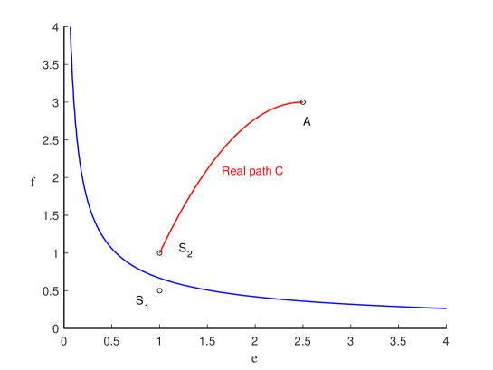
Figure 1: Partitions of the parameter space of Model 1 and sample points

Notice the two points $S_{2}$ and $A$ in Figure 1. One can find a real path $C$ from $A$ to $S_{2}$ such that it does not pass through the blue curve. According to Lemma 2, system (6) has the same number of real roots with the parameters evaluated at $S_{2}$ and $A$. This means that the number of real solutions of system (6) is invariant in the northeast region. Therefore, we can choose a sample point from each region to determine the root number. For this simple system, sample points might be selected directly by eyes, e.g., $S_{1}=(1,1/2)$, $S_{2}=(1,1)$. However, the choosing process might be extremely complex in general, which could be done automatically by using, e.g., the method of partial cylindrical algebraic decomposition or called the PCAD method [Collins1991P].

For each region, one can determine the root number by counting roots of the non-parametric system of (6) evaluated at the corresponding sample point. Take $S_{1}$ as an example, where (6) becomes

$$\left\{x^{3}-1=0,~{}2-\frac{3}{2}x^{2}>0,~{}x>0\right\}.$$ (7)

In order to count the number of its real roots, an obvious way is directly solving $x^{3}-1=0$, i.e., $x=1$, and then checking whether $2-\frac{3}{2}x^{2}>0$ and $x>0$ are satisfied. The result is true, which means that there exists one unique real solution of (7). However, it is difficult to precisely obtain all real zeros of a general univariate system since root formulae do not exist for polynomials with degrees greater than $4$. Therefore, a more systematic method called real root counting [Xia2002A] is generally needed here, and we demonstrate how this method works by using (7) as an example.

It is noted that $x^{3}-1$, $2-\frac{3}{2}x^{2}$ and $x$ have no common zeros, i.e., they have no factors in common. Otherwise, one needs to reduce the common factors from the inequalities first. After that, we isolate all real zeros of $2-\frac{3}{2}x^{2}$ and $x$ by rational intervals, e.g.,

$$\left[-\frac{12}{10},-\frac{11}{10}\right],~{}\left[-\frac{1}{10},\frac{1}{10}\right],~{}\left[\frac{11}{10},\frac{12}{10}\right].$$ (8)

Although it is trivial for this simple example, the isolation process could be particularly tough for general polynomials, which may be handled by using, e.g., the modified Uspensky algorithm [Collins1983R]. Moreover, the intervals can be made as small as possible to guarantee no zeros of $x^{3}-1$ lie in these intervals, which could be checked by using, e.g., Sturm’s theorem [Sturmfels2002S]. Thus, the real zeros of $x^{3}-1$ must be in the complement of (8):

$$\left(-\infty,-\frac{12}{10}\right),~{}\left(-\frac{11}{10},-\frac{1}{10}\right),~{}\left(\frac{1}{10},\frac{11}{10}\right),~{}\left(\frac{12}{10},+\infty\right).$$ (9)

In each of these open intervals, the signs of $2-\frac{3}{2}x^{2}$ and $x$ are invariant and can be determined by checking them at selected sample points. For instance, to determine the sign of $2-\frac{3}{2}x^{2}$ on $(12/10,+\infty)$, we check the sign at a sample point, e.g., $x=2$. We have that $2-\frac{3}{2}x^{2}|_{x=2}=-4<0$, thus $2-\frac{3}{2}x^{2}<0$ on $(12/10,+\infty)$. Similarly, it is obtained that the signs of $2-\frac{3}{2}x^{2}$ and $x$ at (9) are $-,+,+,-$ and $-,-,+,+$, respectively. Hence, $(1/10,11/10)$ is the only interval such that the two inequalities $2-\frac{3}{2}x^{2}>0$ and $x>0$ of system (7) are simultaneously satisfied.

We focus on $(1/10,11/10)$. Using Sturm’s theorem, we can count the number of the real zeros of $x^{3}-1$ at $(1/10,11/10)$, which is one. Therefore, system (6) has one real root at $S_{1}=(1,1/2)$. The above approach works well for a system formulated with univariate polynomial equations and inequalities although some steps seem silly and not necessary for this simple example. Similarly, we know that system (6) has no real roots at $S_{2}=(1,1)$.

In conclusion, system (6) has one real root if the parameters take values from the southwest region where $S_{1}$ lies, and has no real roots if the parameters take values from the northeast region where $S_{2}$ lies. Furthermore, the inequalities of some factors of the border polynomial may be used to explicitly describe a given region. It is evident that $27e^{2}f^{3}-8<0$ describes the region where $S_{1}$ lies. Therefore, Model 1 has one unique stable equilibrium provided that

$$e^{2}f^{3}=\left(\frac{a-c}{4b}\right)^{2}(4bK)^{3}=4b(a-c)^{2}K^{3}<\frac{8}{27},$$

which is consistent with Proposition 1.

According to the classical bifurcation theory, for a one-dimensional iteration map $x(t+1)=F(x(t))$, we know that bifurcations may occur if

$$\left|\frac{{\rm d}x(t+1)}{{\rm d}x(t)}\bigg{|}_{x(t)=x}\right|=\left|\frac{{\rm d}F}{{\rm d}x}\right|=1.$$

More specifically, if ${\rm d}F/{\rm d}x=-1$, then the system may undergo a period-doubling bifurcation (also called flip bifurcation), where the dynamics switch to a new behavior with twice the period of the original system. On the other hand, if ${\rm d}F/{\rm d}x=1$, then the system may undergo a saddle-node (fold), transcritical, or pitchfork bifurcation. One might determine the type of bifurcation from the change in the number of the (stable) equilibria. In the case of saddle-node bifurcation, one stable equilibrium (a node) annihilates with another unstable one (a saddle). Before and after a transcritical bifurcation, there is one unstable and one stable equilibrium, and the unstable equilibrium becomes stable and vice versa. In the case of pitchfork bifurcation, the number of equilibria changes from one to three or from three to one, while the number of stable equilibria changes from one to two or from one to zero. Accordingly, it is concluded that Model 1 may undergo a period-doubling bifurcation if

$$e^{2}f^{3}=4b(a-c)^{2}K^{3}=\frac{8}{27},$$

and there are no other bifurcations.

3.2 Model 2

According to (3), by setting $x(t+1)=x(t)=x$, we know that Model 2 has at most three equilibria. The analytical expressions of the equilibria exist, but are complex, i.e.,

$$\begin{split}x_{1}=\,&{\frac{\sqrt[3]{M}}{12d}}-{\frac{8bd-3{c}^{2}}{4d\sqrt[3]{M}}}+{\frac{c}{4d}},\\ x_{2,3}=\,&-{\frac{\sqrt[3]{M}}{24d}}+{\frac{8bd-3{c}^{2}}{8d\sqrt[3]{M}}}+{\frac{c}{4d}}\pm\frac{\operatorname{i}\sqrt{3}}{2}\left({\frac{\sqrt[3]{M}}{12d}}+{\frac{8bd-3{c}^{2}}{4d\sqrt[3]{M}}}\right),\end{split}$$ (10)

where

$$M=12d\sqrt{3}\sqrt{108{a}^{2}{d}^{2}-108abcd+27\,a{c}^{3}+32{b}^{3}d-9{b}^{2}{c}^{2}}+216a{d}^{2}-108bcd+27{c}^{3}.$$

Furthermore, an equilibrium $x$ is locally stable provided that

$$\left|\frac{{\rm d}x(t+1)}{{\rm d}x(t)}\bigg{|}_{x(t)=x}\right|=\left|1+K(-2b+6cx-12dx^{2})\right|<1.$$

Hence, a stable equilibrium of map (3) is a real solution of

$$\left\{\begin{split}&x=x+K(a-2bx+3cx^{2}-4dx^{3}),\\ &K(-2b+6cx-12dx^{2})<0,\\ &2+K(-2b+6cx-12dx^{2})>0,\\ &x>0,~{}a>0,~{}b>0,~{}c>0,~{}d>0.\end{split}\right.$$ (11)

Obviously, analyzing the stable equilibrium by substituting the closed-form solutions (10) into (11) is complicated and impractical. In comparison, the approach applied in the analysis of Model 1 does not require explicitly solving any closed-form equilibrium. If the analytical solution has a complicated expression or even if there are no closed-form solutions, our approach still works in theory.

Concerning the border polynomial of system (11), we compute

$$\operatorname{discr}(K(a-2bx+3cx^{2}-4dx^{3}))=-16K^{5}dR_{1},$$

$$\operatorname{res}(K(a-2bx+3cx^{2}-4dx^{3}),K(-2b+6cx-12dx^{2}))=-16K^{5}dR_{1},$$

$$\operatorname{res}(K(a-2bx+3cx^{2}-4dx^{3}),2+K(-2b+6cx-12dx^{2}))=-16K^{2}dR_{2},$$

$$\operatorname{res}(K(a-2bx+3cx^{2}-4dx^{3}),x)=-Ka,$$

where

$$R_{1}=\, 108a^{2}d^{2}-108abcd+27ac^{3}+32b^{3}d-9b^{2}c^{2},$$

$$R_{2}=\, 108K^{3}a^{2}d^{2}-108K^{3}abcd+27K^{3}ac^{3}+32K^{3}b^{3}d-9K^{3}b^{2}c^{2}-24Kbd+9Kc^{2}-8d.$$

Therefore, the border polynomial is $-16384\,d^{4}K^{14}aR_{1}^{2}R_{2}$, the zeros of which divide the parameter set $\{(a,b,c,d,K)\,|\,a,b,c,d,K>0\}$ into separated regions. The PCAD method [Collins1991P] permits us to select at least one sample point from each region. In Table 1, we list the 30 selected sample points and the corresponding numbers of distinct real solutions of system (11).

Table 1: Selected Sample Points in $\{(a,b,c,d,K)\,|\,a,b,c,d,K>0\}$

$(a,b,c,d,K)$	num	$R_{1}$	$R_{2}$	$(a,b,c,d,K)$	num	$R_{1}$	$R_{2}$
$(1,1,1/4,1/64,1/2)$	2	$-$	$-$	$(1,1,1/4,1/64,1)$	1	$-$	$+$
$(1,1,1/4,1/64,2)$	0	$-$	$-$	$(1,1,1/4,19/1024,1)$	2	$-$	$-$
$(1,1,1/4,19/1024,2)$	1	$-$	$+$	$(1,1,1/4,19/1024,3)$	0	$-$	$-$
$(1,1,1/4,1/16,1)$	1	$+$	$-$	$(1,1,1/4,1/16,2)$	0	$+$	$+$
$(1,1,1/4,1,1/2)$	1	$+$	$-$	$(1,1,1/4,1,1)$	0	$+$	$+$
$(1,1,3/8,1/64,1/8)$	1	$+$	$-$	$(1,1,3/8,1/64,1)$	0	$+$	$+$
$(1,1,3/8,1/32,1/4)$	2	$-$	$-$	$(1,1,3/8,1/32,1)$	1	$-$	$+$
$(1,1,3/8,1/32,17)$	0	$-$	$-$	$(1,1,3/8,49/1024,1)$	2	$-$	$-$
$(1,1,3/8,49/1024,4)$	1	$-$	$+$	$(1,1,3/8,49/1024,8)$	0	$-$	$-$
$(1,1,3/8,1/16,1)$	1	$-$	$+$	$(1,1,3/8,1/16,3)$	0	$-$	$-$
$(1,1,3/8,1,1/2)$	1	$+$	$-$	$(1,1,3/8,1,1)$	0	$+$	$+$
$(1,1,15/32,1/16,1/2)$	1	$+$	$-$	$(1,1,15/32,1/16,1)$	0	$+$	$+$
$(1,1,15/32,3/32,1)$	1	$+$	$-$	$(1,1,15/32,3/32,8)$	0	$+$	$+$
$(1,1,15/32,1,1/2)$	1	$+$	$-$	$(1,1,15/32,1,1)$	0	$+$	$+$
$(1,1,1,1,1/2)$	1	$+$	$-$	$(1,1,1,1,1)$	0	$+$	$+$

According to Table 1, one can see that system (11) has one real solution if and only if $R_{1}<0,R_{2}>0$ or $R_{1}>0,R_{2}<0$. Moreover, a necessary condition that system (11) has two real solutions is that $R_{1}<0$ and $R_{2}<0$, which is not a sufficient condition, however. For example, at $(a,b,c,d,K)=(1,1,1/4,1/64,2)$, system (11) has no real solutions but $R_{1}<0$ and $R_{2}<0$ are fulfilled. To acquire the necessary and sufficient condition, additional polynomials ($R_{3}$ and $R_{4}$) are needed, which can be found in the so-called generalized discriminant list and can be picked out by repeated trials. Regarding the generalized discriminant list, readers may refer to [Yang2001A] for more details. Due to space limitations, we directly report below the necessary and sufficient condition that system (11) has two real solutions without giving the calculation details:

$$R_{1}<0,R_{2}<0,R_{3}>0,R_{4}<0,$$

where

$$R_{3}=\, 8Kbd-3Kc^{2}+8d,$$

$$R_{4}=\, 432K^{2}a^{2}d^{3}-432K^{2}abcd^{2}+108K^{2}ac^{3}d+128K^{2}b^{3}d^{t}2-36K^{2}b^{2}c^{2}d+192Kb^{2}d^{2}$$

$$-144Kbc^{2}d+27Kc^{4}+64bd^{2}-24c^{2}d.$$

We continue to analyze the bifurcations of this model. An equilibrium $x$ of map (3) may undergo a period-doubling bifurcation if

$$\frac{{\rm d}x(t+1)}{{\rm d}x(t)}\bigg{|}_{x(t)=x}=1+K(-2b+6cx-12dx^{2})=-1.$$

Hence, a period-doubling bifurcation may occur if the following system has at least one real solution.

$$\left\{\begin{split}&x=x+K(a-2bx+3cx^{2}-4dx^{3}),\\ &K(-2b+6cx-12dx^{2})+2=0,\\ &x>0,~{}a>0,~{}b>0,~{}c>0,~{}d>0.\end{split}\right.$$ (12)

By using the method of triangular decomposition, we transform the solutions of the first two equations of system (12) into zeros of the triangular set

$$\mathcal{T}=[(8Kbd-3Kc^{2}+4d)x-6adK+bcK-c,R_{2}].$$

Obviously, the system $\{\mathcal{T}=0,~{}x>0,~{}a>0,~{}b>0,~{}c>0,~{}d>0\}$ has at least one real positive solution if $R_{2}=0$ and $x=(6adK-bcK+c)/(8Kbd-3Kc^{2}+4d)>0$, i.e.,

$$R_{2}=0,~{}R_{5}>0,$$

where

$$R_{5} =\,(6adK-bcK+c)(8Kbd-3Kc^{2}+4d)$$

$$=\,48K^{2}abd^{2}-18K^{2}ac^{2}d-8K^{2}b^{2}cd+3K^{2}bc^{3}+24Kad^{2}+4Kbcd-3Kc^{3}+4cd.$$

Similarly, concerning the occurrence of a pitchfork bifurcation, we consider

$$\left\{\begin{split}&x=x+K(a-2bx+3cx^{2}-4dx^{3}),\\ &K(-2b+6cx-12dx^{2})=0,\\ &x>0,~{}a>0,~{}b>0,~{}c>0,~{}d>0,\end{split}\right.$$ (13)

and count the number of stable equilibria. More details are not reported here due to space limitations. We summarize all the obtained results in the following theorem.

Theorem 1.

Model 2 has at most two stable equilibria. Specifically, there exists just one stable equilibrium if

$$R_{1}<0,R_{2}>0~{}\text{or}~{}R_{1}>0,R_{2}<0,$$

and there exist two stable equilibria if

$$R_{1}<0,R_{2}<0,R_{3}>0,R_{4}<0.$$

Moreover, there is a period-doubling bifurcation if

$$R_{2}=0,~{}R_{5}>0,$$

and there is a pitchfork bifurcation if

$$R_{1}=0,~{}R_{2}>0,~{}R_{6}>0~{}\text{or}~{}R_{1}=0,~{}R_{2}>0,~{}R_{4}<0,~{}R_{6}>0,$$

where

$$R_{6}=\, 48abd^{2}-18ac^{2}d-8b^{2}cd+3bc^{3}.$$