A new over-dispersed count model

Abstract

A new two-parameter discrete distribution, namely the $PoiG$ distribution is derived by the convolution of a Poisson variate and an independently distributed geometric random variable. This distribution generalizes both the Poisson and geometric distributions and can be used for modelling over-dispersed as well as equi-dispersed count data. A number of important statistical properties of the proposed count model, such as the probability generating function, the moment generating function, the moments, the survival function and the hazard rate function. Monotonic properties are studied such as the log concavity and the stochastic ordering are also investigated in detail. Method of moment and the maximum likelihood estimators of the parameters of the proposed model are presented. It is envisaged that the proposed distribution may prove to be useful for the practitioners for modelling over-dispersed count data compared to its closest competitors.

Keywords Geometric distribution, Poisson distribution, Conway-Maxwell Poisson distribution; $BerG$ distribution; $BerPoi$ distribution; Incomplete gamma function.

MSC 2010 60E05, 62E15.

1 Introduction

The phenomenon of the variance of a count data being more than its mean is commonly termed as over-dispersion in the literature. Over-dispersion is relevant in many modelling applications and it is encountered more often compared to the phenomena of under-dispersion and equi-dispersion. A number of count models are available in the literature for over-dispersed data. However, addition of a simple yet adequate model is of importance given the ongoing research interest in this direction ([37], [25], [32], [35], [30], [29], [9], [19], [26], [34], [5], [2] and [36]). The simplest and the most common count data model is the Poisson distribution. Its equi-dispersion characteristic is well-known. This is a limitation for the Poisson model and to overcome this issue, several alternatives have been developed and used for their obvious advantage over the classical Poisson model. Notable among these distributions are the hyper-Poisson (HP) of Bardwell and Crow [6], generalized Poisson distribution of Jain and Consul [20], double-Poisson of Efron [16], weighted Poisson of Castillo and Pérez-Casany [15], weighted generalized Poisson distribution of Chakraborty [10], Mittag-Leffler function distribution of Chakraborty and Ong [13] and the popular COM-Poisson distribution Shmueli et al. [31]. COM-Poisson generalizes the binomial and the negative binomial distribution. The classical geometric and negative binomial models are also used for over-dispersed count datasets. The gamma mixture of the Poisson distribution generates the negative binomial distribution [17]. Thus unlike the Poisson distribution, these two count models posses the over-dispersion characteristic. Consequently, several extensions of the geometric distribution have been introduced in the literature for over-dispersed count data modelling ([11], [12], [18], [20], [22], [27], [28], and [33] among others). Two most widely used distributions for over-dispersed data are of course the negative binomial and COM-Poisson. As pointed out earlier, there is still plenty of opportunity for developing new discrete distributions with simple structure and explicit interpretation, appropriate for over-dispersed data.

Recently, Bourguignon et al. have introduced the $BerG$ distribution [8] by using the convolution of a Bernoulli random variable and a geometric random variable. In a very recent publication, Bourguignon et al. have introduced the $BerPoi$ distribution from a similar motivation [7]. This is a convolution of a Bernoulli random variable and a Poisson random variable. The first one is capable of modelling over-dispersed, under-dispersed and equi-dispersed data whereas the second one is efficient for modelling under-dispersed data. This approach is simple and has enormous potential. Here we use this idea to develop a novel over-dispersed count model.

In this article, we propose a new discrete distribution derived from the convolution of two independent count random variables. The random variables are Poisson and geometric. Hence we identify the proposed model as $PoiG$. This two-parameter distribution has many advantages. Structural simplicity is one of them. It is easy to comprehend unlike the COM-Poisson distribution, which involves a difficult normalising constant in its probability mass function. A model with closed-form expressions of the mean and the variance is well-suited for regression modelling. Unlike the COM-Poisson distribution, mean and variance of the proposed distribution can be written in closed form expressions. The proposed distribution extends both the Poisson and geometric distributions.

Rest of the article is organized as follows. In section 2, we present the $PoiG$ distribution. In Section 3, we describe its important statistical properties such as recurrence relation, generating functions, moments, dispersion index, mode, reliability properties, monotonic properties and stochastic ordering. In Section 4, we present the moment and the maximum likelihood methods of parameter estimation. We conclude the article with a few limitations and future scopes of the current study.

2 The $PoiG$ distribution

In this section, we introduce a novel discrete distribution by considering two independent discrete random variables $Y_{1}$ and $Y_{2}$. Let us denote the set of non-negative integers, $\{0,1,2,...\}$ by $N_{0}$. Also let, $Y_{1}$ and $Y_{2}$ follow the Poisson distribution with mean $\lambda>0$ and the geometric distribution with mean $0<1/\theta<1$, respectively. Both $Y_{1}$ and $Y_{2}$ have the same support $N_{0}$. For convenience, we write $Y_{1}\sim P(\lambda)$ and $Y_{2}\sim G(\theta)$. Consider, $Y=Y_{1}+Y_{2}$. Then,

$$\Pr(Y=y) =\sum_{i=0}^{y}\Pr(Y_{1}=i)\Pr(Y_{2}=y-i)$$

$$=\sum_{i=0}^{y}\dfrac{e^{-\lambda}\lambda^{i}}{i!}\theta(1-\theta)^{y-i}$$

$$=\theta(1-\theta)^{y}e^{-\lambda}\sum_{i=0}^{y}\dfrac{1}{i!}\left(\dfrac{\lambda}{1-\theta}\right)^{i},\hskip 40.0pty=0,1,2,...\,\,.$$ (1)

The distribution in (2) being the convolution Poisson and geometric, is named the $PoiG$ distribution and we write $Y\sim PoiG(\lambda,\theta)$. Thus, the probability mass function (pmf) of $PoiG(\lambda,\theta)$ can be written as

$$p_{Y}(y) =\dfrac{\theta{(1-\theta)^{y}}}{\Gamma(y+1)}\exp{\left(\dfrac{\lambda\theta}{1-\theta}\right)}{\Gamma\left(y+1,\dfrac{\lambda}{1-\theta}\right)},\hskip 30.0pty=0,1,2,...\,\,.$$ (2)

Figure 1 exhibits nature of the pmf for different choices of $(\lambda,\theta)$. The cumulative distribution function (cdf) of $PoiG$ distribution is

$$F_{Y}(y) =\Pr(Y_{1}+Y_{2}\leq y)$$

$$=\sum_{y_{1}=0}^{y}\sum_{y_{2}=0}^{y-y_{1}}p_{Y}(y_{1})p_{Y}(y_{2})$$

$$=\sum_{y_{1}=0}^{y}F_{G}(y-y_{1})p_{Y}(y_{1})$$

$$=\sum_{y_{1}=0}^{y}(1-(1-\theta)^{y-y_{1}+1})p_{Y}(y_{1})$$

$$=\sum_{y_{1}=0}^{y}\dfrac{e^{-\lambda}\lambda^{y_{1}}}{y_{1}!}-(1-\theta)^{y+1}e^{-\lambda}\sum_{y_{1}=0}^{y}\dfrac{1}{y_{1}!}\left(\dfrac{\lambda}{1-\theta}\right)^{y_{1}}.$$ (3)

An explicit expression of (2) is given by

$$F_{Y}(y) =\dfrac{\Gamma(y+1,\lambda)}{\Gamma(y+1)}-\dfrac{(1-\theta)^{y+1}}{\Gamma(y+1)}\exp{\left(\dfrac{\lambda\theta}{1-\theta}\right)}\Gamma\left(y+1,\dfrac{\lambda}{1-\theta}\right),\hskip 25.0pty=0,1,2,...\,\,.$$ (4)

Figure 2 exhibits nature of the cdf for different choices of $(\lambda,\theta)$. The mean and variance of the $PoiG(\lambda,\theta)$ distribution are given as follows.

$$E(Y)=\mu=\lambda+\dfrac{1-\theta}{\theta}\hskip 10.0pt\textrm{and}\hskip 10.0ptV(Y)=\sigma^{2}=\lambda+\dfrac{1-\theta}{\theta^{2}}$$ (5)

Special cases

• For $\lambda\xrightarrow{}0$, $PoiG(\lambda,\theta)$ behaves like $G(\theta)$.

• For $\theta\xrightarrow{}1$, $PoiG(\lambda,\theta)$ behaves like $P(\lambda)$.

Remark 1

• The incomplete gamma function [1] is defined as $\Gamma(n,x)=\int_{x}^{\infty}t^{(n-1)}e^{-t}dt$ and it can also be rewrite as $\Gamma(n,x)=(n-1)!\sum_{k=0}^{n-1}\dfrac{e^{-x}x^{k}}{k!}$, which is valid for positive values of $n$ and any value of $x$. Thus the incomplete gamma function in (2) can be rewritten as

  $$\Gamma\left(y+1,\dfrac{\lambda}{1-\theta}\right) =\Gamma(y+1){\sum_{i=0}^{y}}\dfrac{1}{\Gamma(i+1)}\exp{\left(-\dfrac{\lambda}{1-\theta}\right)}{\left(\dfrac{\lambda}{1-\theta}\right)^{i}},$$

  where $\Gamma(y+1)=y!$ and $\Gamma(i+1)=i!$.

• $F_{Y}(0)=p_{Y}(0)=\theta e^{-\lambda}$. Thus, the proportion of zeros in case of the $PoiG$ distribution tends to $\theta$ as $\lambda\rightarrow 0$ and to zero as $\lambda\rightarrow\infty$.

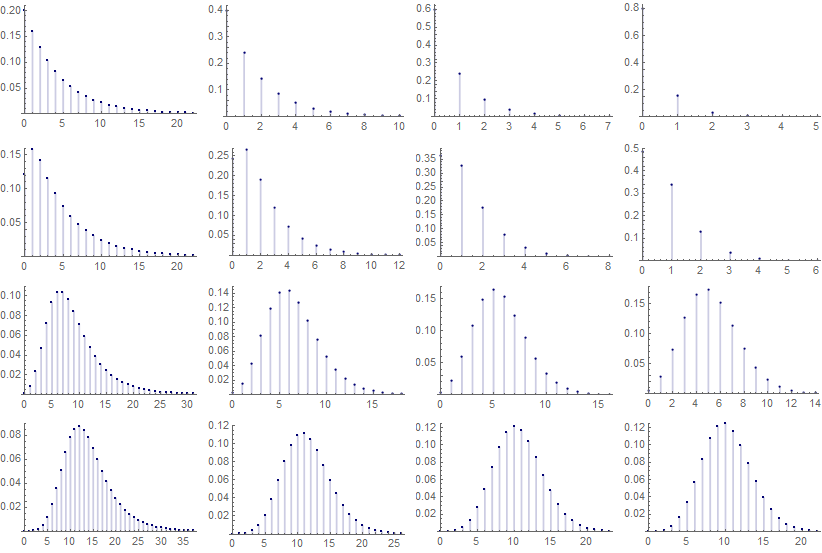
Figure 1: Probability mass function of $PoiG(\lambda,\theta)$ for $\lambda\in\{0,0.5,5,10\}$ and $\theta\in\{0.2,0.4,0.6,0.8\}$. The $(i,j)^{th}$ plot corresponds to the $i^{th}$ value of $\lambda$ and $j^{th}$ value of $\theta$ for $i,j=1,2,3,4$.

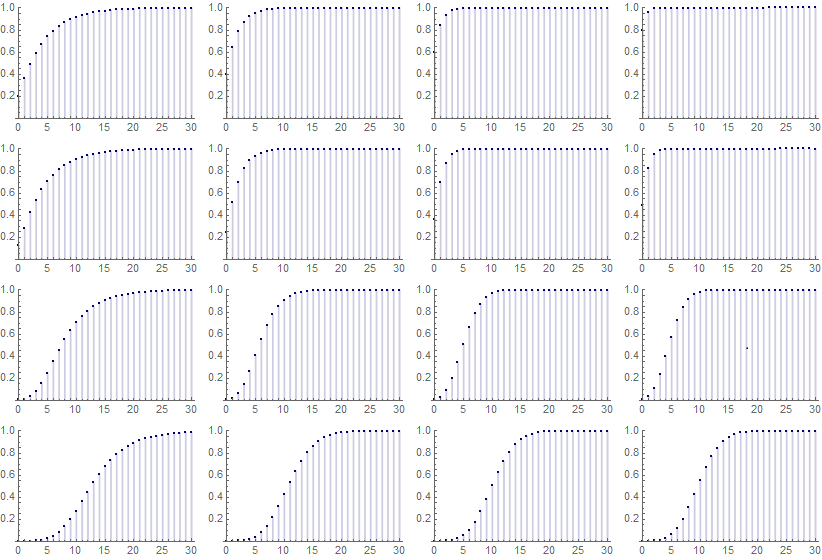
Figure 2: Cumulative distribution function of $PoiG(\lambda,\theta)$ for $\lambda\in\{0,0.5,5,10\}$ and $\theta\in\{0.2,0.4,0.6,0.8\}$ .The $(i,j)^{th}$ plot corresponds to the $i^{th}$ value of $\lambda$ and $j^{th}$ value of $\theta$ for $i,j=1,2,3,4$.

3 Properties of the $PoiG$ distribution

In this section, we explore several important statistical properties of the proposed $PoiG(\lambda,\theta)$ distribution. Some of the distributional properties studied here are the recurrence relation, probability generating function (pgf), moment generating function (mgf), characteristic function (cf), cumulant generating function (cgf), moments, coefficient of skewness and kurtosis. We also study the reliability properties such as the survival function and the hazard rate function. Log-concavity and stochastic ordering of the proposed model are also investigated.

3.1 Recurrence relation

Probability recurrence relation helps in finding the subsequent term using the preceding term. It usually proves to be advantageous in computing the masses at different values. Note that,

$$p_{Y}(y) =\dfrac{\theta{(1-\theta)^{y}}}{\Gamma(y+1)}\exp{\left(\dfrac{\lambda\theta}{1-\theta}\right)}{\Gamma\left(y+1,\dfrac{\lambda}{1-\theta}\right)}$$

$$=\theta{(1-\theta)^{y}}e^{-\lambda}\sum_{i=0}^{y}\dfrac{1}{\Gamma(i+1)}\left(\dfrac{\lambda}{1-\theta}\right)^{i}$$

$$=\theta{(1-\theta)^{y}}e^{-\lambda}s_{y}.$$

Where,

$$s_{y}=\sum_{i=0}^{y}\dfrac{1}{\Gamma(i+1)}\left(\dfrac{\lambda}{1-\theta}\right)^{i}$$

and

$$s_{y+1}=s_{y}+\dfrac{1}{\Gamma(y+2)}\left(\dfrac{\lambda}{1-\theta}\right)^{y+1}.$$

Now,

$$p_{Y}(y+1) =\theta{(1-\theta)^{y+1}}e^{-\lambda}s_{y+1}$$

$$=\theta{(1-\theta)^{y+1}}e^{-\lambda}\left[s_{y}+\dfrac{1}{\Gamma(y+2)}\left(\dfrac{\lambda}{1-\theta}\right)^{y+1}\right]$$

$$=(1-\theta)p_{Y}(y)+\theta e^{-\lambda}\dfrac{{\lambda}^{y+1}}{\Gamma(y+2)}.$$ (6)

This is the recurrence formula of the $PoiG$ distribution. It is easy to check that

$$\dfrac{s_{y+1}}{s_{y}} =1+\dfrac{1}{s_{y}\Gamma(y+2)}\left(\dfrac{\lambda}{1-\theta}\right)^{y+1}=1\hskip 25.0ptas\hskip 5.0pty\xrightarrow{}\infty,$$

and

$$\dfrac{p_{Y}(y+1)}{p_{Y}(y)} =(1-\theta)+\dfrac{\theta e^{-\lambda}}{p_{Y}(y)}\dfrac{\lambda^{y+1}}{\Gamma(y+2)}=1-\theta\hskip 25.0ptas\hskip 5.0pty\xrightarrow{}\infty.$$ (7)

From (7), it is clear that the behaviour of the tail of the distribution depends on $\theta$. When $\theta\xrightarrow{}0$, the tail of the distribution decays relatively slowly, which implies long tail. when $\theta\xrightarrow{}1$, the tail of the distribution decays fast, which implies short tail. This can easily be verified from Figure 1.

3.2 Generating functions

We use the notation $H$ to denote a pgf and use the notation of the corresponding random variable in the subscript. For $Y_{1}\sim P(\lambda)$ and $Y_{2}\sim G(\theta)$,

$$H_{Y_{1}}(s) =e^{\lambda(s-1)}\hskip 10.0pt\textrm{and}\hskip 10.0ptH_{Y_{2}}(s)=\dfrac{\theta}{1-(1-\theta)s}.$$

Now by using the convolution property of probability generating function we obtain the pgf of $PoiG(\lambda,\theta)$ as

$$H_{Y}(s) =\dfrac{\theta e^{\lambda(s-1)}}{1-s+\theta s}.$$ (8)

Similar methods are used to obtain the other generating functions, including the mgf $M_{Y}(t)$, cf $\phi_{Y}(t)$ and cgf $K_{Y}(t)$. These are given below.

$$M_{Y}(t)=\dfrac{\theta e^{\lambda(t-1)}}{1-(1-\theta)t}$$ (9)

$$\phi_{Y}(t) =\dfrac{\theta e^{\lambda(e^{it}-1)}}{1-(1-\theta)e^{it}}$$ (10)

$$K_{Y}(t) =\lambda(e^{t}-1)+log\left\{\dfrac{\theta}{1-(1-\theta)e^{t}}\right\}$$ (11)

Let us discuss some useful definitions and notations for Result 1 given below. The notation $G(\theta)$ has already been introduced in Section 2. Let $R$ be the number of failures preceding the first success in a sequence of independent Bernoulli trials. If the probability of success is $\theta\in(0,1)$, then $R$ is said to follow $G(\theta)$. Suppose, we wait for the $r^{th}$ success. Then the number of failures is a negative binomial random variable with index $r$ and the parameter $\theta$. Let $NB(r,\theta)$ denote this distribution. Suppose $R_{i}\sim G(\theta)$, for $i=1,2,...,r$ independently and $S\sim NB(r,\theta)$. Then $S=R_{1}+R_{2}+...+R_{r}$. Thus, it is clear that the $G(\theta)$ is a particular case of $NB(r,\theta)$ with $r=1$. Similar to the genesis of $PoiG$ model, if we add one Poisson random variable and an independently distributed negative binomial random variable, it is possible to obtain a generalization of the $PoiG$ model. An appropriate notation for this distribution would have been $PoiNB$. The objective of the current work is not to study this three-parameter distribution in detail. However, the following result establishes that the generalization from the geometric distribution to the negative binomial distribution translates similarly to the $PoiG-PoiNB$ case. This may prove to be a motivation for generalizing the proposed model to $PoiNB$ in future.

Result 1 The distribution of the sum of $n$ independent $PoiG$ random variables is a $PoiNB$ random variable for fixed $\theta$. Mathematically, if $Y_{i}\sim PoiG(\lambda_{i},\theta)$ for each $i=1,2,...,n$ then,

$$\sum_{i=1}^{n}Y_{i}\sim PoiNB(\sum_{i=1}^{n}\lambda_{i},n,\theta).$$

Proof of Result 1 From (8), the pgf of $Y_{i}\sim PoiG(\lambda_{i},\theta)$ is

$$H_{Y_{i}}(s) =\dfrac{\theta e^{\lambda_{i}(s-1)}}{1-s+\theta s}$$

for $i=1,2,...,n$. We can derive the pgf of sum of $n$ independent $PoiG(\lambda_{i},\theta)$ variates based on the convolution property of the pgf. Let, $Z=Y_{1}+Y_{2}+....+Y_{n}$. Then,

$$H_{Z}(s) =\prod_{i=1}^{n}H_{Y_{i}}(s)$$

$$=\dfrac{\theta^{n}}{(1-s+\theta s)^{n}}e^{\sum_{i=1}^{n}{\lambda_{i}(s-1)}}.$$ (12)

The term $\theta^{n}/(1-s+\theta s)^{n}$ in (3.2) is the pgf of $NB(n,\theta)$ which is a generalisation of geometric distribution and $e^{\sum_{i=1}^{n}{\lambda_{i}(s-1)}}$ is pgf of $P\left(\sum_{i=1}^{n}\lambda_{i}\right)$. Thus $\sum_{i=1}^{n}Y_{i}\sim PoiNB\left(\sum_{i=1}^{n}\lambda_{i},n,\theta\right)$.

3.3 Moments and related concepts

The $r^{th}$ order raw moment of $Y\sim PoiG(\lambda,\theta)$ can be obtained using the general expressions of the raw moments of $Y_{1}\sim P(\lambda)$ and $Y_{2}\sim G(\theta)$ as follows.

$$E(Y^{r}) =E\left(\sum_{j=0}^{r}\binom{Y}{j}{Y_{1}}^{j}{Y_{2}}^{y-j}\right)$$

$$=\sum_{j=0}^{r}\binom{Y}{j}E({Y_{1}}^{j})E({Y_{2}}^{y-j})$$

Note that,

$$E({Y_{1}}^{j}) =\sum_{{Y_{1}}=0}^{\infty}{Y_{1}}^{j}\hskip 5.0pt\dfrac{e^{-\lambda}{\lambda}^{Y_{1}}}{Y_{1}!}$$

$$=\sum_{{Y_{1}}=0}^{\infty}\lambda^{Y_{1}}S(j,{Y_{1}})$$

$$=\phi_{j}(\lambda).$$

Here, $S(j,{Y_{1}})$ is the Stirling number of the second kind [1] and $\phi_{j}(\lambda)$ is the Bell polynomial [24]. Again,

$$E({Y_{2}}^{y-j}) =\sum_{{Y_{2}}=0}^{\infty}{Y_{2}}^{y-j}\theta(1-\theta)^{Y_{2}}$$

$$=\theta\hskip 5.0ptLi_{-(y-j)}(1-\theta),$$

where $Li_{-(y-j)}(1-\theta)$ is the polylogarithm of negative integers [14]. Hence

$$E(Y^{r}) =\sum_{j=0}^{r}\binom{Y}{j}\phi_{j}(\lambda)\theta\hskip 5.0ptLi_{-(y-j)}(1-\theta).$$ (13)

The $r^{th}$ order raw moment can also be calculated by differentiating the mgf in (9) $r$ times with respect to $t$ and putting $t=0$. That is,

$$E(Y^{r})=M_{Y}^{(r)}(0)=\dfrac{d^{r}}{dt^{r}}[M_{Y}(t)]_{t=0}.$$

Explicit expressions of the first four moments are listed below.

$$E(Y) =\lambda+\dfrac{1-\theta}{\theta}$$ (14)

$$E(Y^{2}) =\dfrac{1}{\theta^{2}}[\theta^{2}(\lambda^{2}-\lambda+1)+\theta(2\lambda-3)+2]$$ (15)

$$E(Y^{3}) =\dfrac{1}{\theta^{3}}[\theta^{3}(\lambda^{3}+\lambda-1)+\theta^{2}(3\lambda^{2}-6\lambda+7)+\theta(6\lambda-12)+6]$$ (16)

$$E(Y^{4}) =\dfrac{1}{\theta^{4}}[\theta^{4}(\lambda^{4}+2\lambda^{3}+\lambda^{2}-\lambda+1)+\theta^{3}(4\lambda^{3}-6\lambda^{2}+14\lambda-15)$$

$$\hskip 30.0pt+2\theta^{2}(6\lambda^{2}-18\lambda+25)+12\theta(2\lambda-5)+24]$$ (17)

Using the above, explicit expressions of the first four central moments are given as follows.

$$\mu_{1} =0$$ (18)

$$\mu_{2} =\lambda+\dfrac{1-\theta}{\theta^{2}}$$ (19)

$$\mu_{3} =\frac{\theta^{3}\lambda+\theta^{2}-3\theta+2}{\theta^{3}}$$ (20)

$$\mu_{4} =\frac{\theta^{4}\lambda(3\lambda+1)-\theta^{3}(6\lambda+1)+2\theta^{2}(3\lambda+5)-18\theta+9}{\theta^{4}}$$ (21)

The first raw and second central moments are mean and variance of the $PoiG(\lambda,\theta)$ distribution, respectively. Let $\gamma_{1}$ and $\gamma_{2}$ denote the coefficients of skewness and kurtosis, respectively. Using the central moments, these coefficients can be derived in closed forms as follows.

$$\beta_{1} =\frac{{\mu_{3}}^{2}}{{\mu_{2}}^{3}}=\frac{\left(\theta^{3}\lambda+\theta^{2}-3\theta+2\right)^{2}}{\left(\theta^{2}\lambda-\theta+1\right)^{3}}$$

$$\gamma_{1} =\sqrt{\beta_{1}}=\sqrt{\frac{\left(\theta^{3}\lambda+\theta^{2}-3\theta+2\right)^{2}}{\left(\theta^{2}\lambda-\theta+1\right)^{3}}}$$

$$\beta_{2} =\frac{\mu_{4}}{{\mu_{2}}^{2}}=\frac{\theta^{4}\lambda(3\lambda+1)-\theta^{3}(6\lambda+1)+2\theta^{2}(3\lambda+5)-18\theta+9}{\left(\theta^{2}\lambda-\theta+1\right)^{2}}$$

$$\gamma_{2} =\beta_{2}-3=\frac{\theta^{4}\lambda(3\lambda+1)-\theta^{3}(6\lambda+1)+2\theta^{2}(3\lambda+5)-18\theta+9}{\left(\theta^{2}\lambda-\theta+1\right)^{2}}-3$$

Remark 3

• As $\theta\rightarrow 1$, $\beta_{1}\rightarrow\dfrac{1}{\lambda}$ and as $\theta\rightarrow 0$, $\beta_{1}\rightarrow 4$.

• As $\theta\rightarrow 1$, $\beta_{2}\rightarrow 3+\dfrac{1}{\lambda}$ and as $\theta\rightarrow 0$, $\beta_{2}\rightarrow 9$.

The statements made in Remark 3 can easily be realized visually from Figure 4 and Figure 4, respectively. Clearly, as $\lambda\rightarrow\infty$, the distribution tends to attain normal shape with $\beta_{1}\rightarrow 0$ and $\beta_{2}\rightarrow 3$.

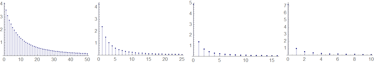
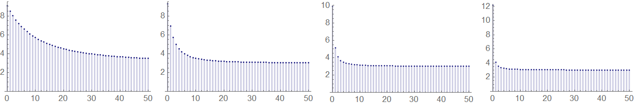
Figure 3: Skewness of $PoiG(\lambda,\theta)$ for $\theta\in\{0.2,0.4,0.6,0.8\}$. The $i^{th}$ plot corresponds to the $i^{th}$ value of $\theta$ for different values of $\lambda$ in the $x$-axis.

Figure 4: Kurtosis of $PoiG(\lambda,\theta)$ for $\theta\in\{0.2,0.4,0.6,0.8\}$. The $i^{th}$ plot corresponds to the $i^{th}$ value of $\theta$ for different values of $\lambda$ in the $x$-axis.

3.4 Dispersion index and coefficient of variation

The  dispersion index determines whether a distribution is suitable for modelling an over, under and equi-dispersed dataset or not. Let $I_{Y}$ denote the dispersion index of the distribution of the random variable $Y$. When $I_{Y}$ is more or less than one, the distribution of $Y$ can accommodate over-dispersion or under-dispersion, respectively. The notion of equi-dispersion is indicated when $I_{Y}=1$. The dispersion index is given by

$$I_{Y} =\dfrac{{\sigma}^{2}}{\mu}=1+\dfrac{(1-\theta)^{2}}{\theta(1+\lambda\theta-\theta)}.$$

From the expression of $I_{Y}$ above, it follows that the $PoiG$ distribution is equi-dispersed when $\theta=1$ and over-dispersed for all $0<\theta<1$. From Figure 5, it can be observed that $I_{Y}$ increases with decreasing $\lambda$ and $\theta$.

The coefficient of variation (CV) is an indicator for data variability. Higher value of the CV indicates the capability of a distribution to model data with higher variability. Note that,

$$CV(Y)=\dfrac{\sqrt{\lambda\theta^{2}-\theta+1}}{\lambda\theta-\theta+1}\times 100\%.$$

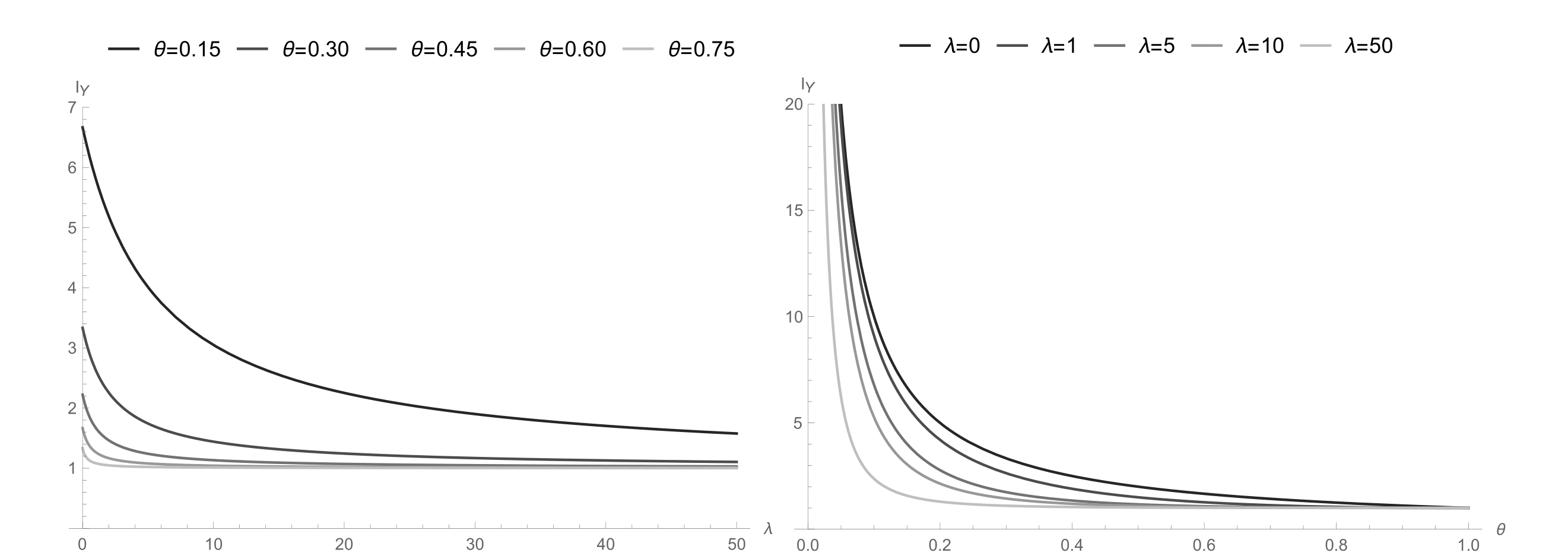
Figure 5: Dispersion index of $PoiG(\lambda,\theta)$.

3.5 Mode

In Section 3.7, we show that $PoiG(\lambda,\theta)$ is unimodal. Note that,

$$p_{Y}(1)\leq p_{Y}(0)$$

$$\implies (1+\lambda-\theta)\theta e^{-\lambda}\leq\theta e^{-\lambda}$$

$$\implies \lambda\theta e^{-\lambda}-\theta^{2}e^{-\lambda}\leq 0$$

$$\implies \lambda-\theta\leq 0$$

$$\implies \lambda\leq\theta.$$

The converse is trivially true. Thus, the distribution has mode at zero for $\lambda\leq\theta$. Figure 1 clearly shows that the mode is zero for $\lambda=0,0.5$ and $\theta>0,0.5$. For the equality case, that is $\lambda=\theta$, the masses at zero and at unity are the same. Figure 6 clearly exhibits this fact. However, for the $\lambda>\theta$ case, the distribution has non-zero mode. Unfortunately, an explicit expression for this non-zero mode is difficult to find, if not impossible.

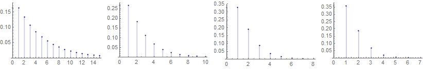
Figure 6: Probability mass function of $PoiG(\lambda,\theta)$ for $\lambda=\theta\in\{0.2,0.4,0.6,0.8\}$.

3.6 Reliability properties

Reliability function of a discrete random variable $Y$ at $y$ is defined as the probability of $Y$ assuming values greater than or equal to $y$. The reliability function is also termed as the survival function. The survival function of $Y\sim PoiG(\lambda,\theta)$ is

$$S_{Y}(y) =P(Y\geq y)=1-\dfrac{\Gamma(y,\lambda)}{\Gamma y}+\dfrac{(1-\theta)^{y}}{\Gamma y}\exp{\left(\dfrac{\lambda\theta}{1-\theta}\right)}\Gamma\left(y,\dfrac{\lambda}{1-\theta}\right).$$ (22)

The hazard rate or failure rate of a discrete random variable $T$ at time point $t$ is defined as the conditional probability of failure at $t$, given that the survival time is at least $t$. The hazard rate function (hrf) of $Y\sim PoiG(\lambda,\theta)$ can be obtained by using (2) and (4) as follows.

$$h_{Y}(y)=\dfrac{P(Y=y)}{P(Y\geq y)} =\dfrac{\dfrac{\theta(1-\theta)^{y}}{\Gamma(y+1)}\exp{\left(\dfrac{\lambda\theta}{1-\theta}\right)}\Gamma\left(y+1,\dfrac{\lambda}{1-\theta}\right)}{1-\dfrac{\Gamma(y,\lambda)}{\Gamma y}+\dfrac{(1-\theta)^{y}}{\Gamma y}\exp{\left(\dfrac{\lambda\theta}{1-\theta}\right)}\Gamma\left(y,\dfrac{\lambda}{1-\theta}\right)}$$

$$=\dfrac{\theta(1-\theta)^{y}\exp{\left(\dfrac{\lambda\theta}{1-\theta}\right)}\Gamma\left(y+1,\dfrac{\lambda}{1-\theta}\right)}{\Gamma(y+1)-y\Gamma(y,\lambda)+y(1-\theta)^{y}\exp{\left(\dfrac{\lambda\theta}{1-\theta}\right)}\Gamma\left(y,\dfrac{\lambda}{1-\theta}\right)}.$$ (23)

The hrf for different choices of the parameters are exhibited in Figure 7. The $PoiG$ distribution exhibits constant failure rate when $\lambda$ is very small and it exhibits an increasing failure rate, up to a specific time period, when $\lambda$ increases.

In reliability studies, the mean residual life is the expected additional lifetime given that a component has survived until a fixed time. If the random variable $Y\sim PoiG(\lambda,\theta)$ represents the life of a component, then the mean residual life is

$$\mu_{Y}(y) =E(Y-y|Y\geq y)$$

$$=\frac{\sum_{y=k}^{\infty}(y-k)P(Y=y)}{P(Y\geq y)}$$

$$=\frac{\sum_{y=k}^{\infty}\bar{F}(y)}{\bar{F}(k-1)}$$

$$=\frac{\sum_{y=k}^{\infty}\left(\ 1-\dfrac{\Gamma(y,\lambda)}{\Gamma y}+\dfrac{(1-\theta)^{y}}{\Gamma y}\exp{\left(\dfrac{\lambda\theta}{1-\theta}\right)}\Gamma\left(y,\dfrac{\lambda}{1-\theta}\right)\right)}{1-\dfrac{\Gamma(k-1,\lambda)}{\Gamma(k-1)}+\dfrac{(1-\theta)^{k-1}}{\Gamma(k-1)}\exp{\left(\dfrac{\lambda\theta}{1-\theta}\right)}\Gamma\left(k-1,\dfrac{\lambda}{1-\theta}\right)}.$$ (24)

3.7 Monotonic Properties

$Y\sim PoiG(\lambda,\theta)$ is log-concave if the following holds for all $y\geq 1$.

$$p_{Y}^{2}(y)\geq p_{Y}(y-1)p_{Y}(y+1)$$

A log-concave distribution possesses several desirable properties. Some of the notable examples of log-concave distributions are the Bernoulli, binomial, Poisson, geometric, and negative binomial. Convolution of two independent log-concave distributions is also a log-concave distribution [21]. Being the convolution of Poisson and Geometric distributions, the proposed $PoiG$ distribution is log-concave. Consequently, the following statements hold good for the $PoiG$ distribution ([23] and [3]).

• Strongly unimodal.

• At most one exponential tail.

• All the moments exist.

• Log-concave survival function.

• Monotonically increasing hazard rate function (see Figure 7).

• Monotonically decreasing mean residual life function.

Figure 7: Hazard rate function of $PoiG(\lambda,\theta)$ for $\lambda\in\{0,0.5,5,10\}$ row-wise and $\theta\in\{0.2,0.4,0.6,0.8\}$ column-wise. The $(i,j)^{th}$ plot corresponds to the $i^{th}$ value of $\lambda$ and $j^{th}$ value of $\theta$ for $i,j=1,2,3,4$.

3.8 Stochastic ordering

Stochastic order is an important statistical property used to compare the behaviour of different random variables [4]. We have considered here the likelihood ratio order $\geq_{lr}$. Let $X\sim PoiG(\lambda_{1},\theta)$ and $Y\sim PoiG(\lambda_{2},\theta)$. Then $Y$ is said to be smaller than $X$ in the usual likelihood ratio order, that is $Y\leq_{lr}X$) if $L(x)=p_{X}(x)/p_{Y}(x)$ is an increasing function in $x$, that is $L(x)\leq L(x+1)$ for all $0<\theta<1$ and $\lambda_{2}<\lambda_{1}$. Note that,

$$p_{X}(x) =\theta(1-\theta)^{x}e^{-\lambda_{1}}\sum_{i=0}^{x}\dfrac{1}{\Gamma(i+1)}\left(\dfrac{\lambda_{1}}{1-\theta}\right)^{i},\hskip 25.0ptx=0,1,2,...$$

$$p_{Y}(x) =\theta(1-\theta)^{x}e^{-\lambda_{2}}\sum_{i=0}^{x}\dfrac{1}{\Gamma(i+1)}\left(\dfrac{\lambda_{2}}{1-\theta}\right)^{i},\hskip 25.0ptx=0,1,2,...\,.$$

$$L(x) =\exp{[-(\lambda_{1}-\lambda_{2})]}\dfrac{\sum_{i=0}^{x}\dfrac{1}{\Gamma(i+1)}\left(\dfrac{\lambda_{1}}{1-\theta}\right)^{i}}{\sum_{i=0}^{x}\dfrac{1}{\Gamma(i+1)}\left(\dfrac{\lambda_{2}}{1-\theta}\right)^{i}},\hskip 12.0ptx=0,1,2,...$$

It is easy to see that, $L(x)\leq L(x+1)$ for all $0<\theta<1$ and $\lambda_{2}<\lambda_{1}$.

Let $Y\leq_{st}X$ denote $P(Y\geq x)\leq P(X\geq x)$ for all $x$. This is the notion of stochastic ordering. Similarly, the hazard rate order $Y\leq_{hr}X$ implies

$$\dfrac{p_{X}(x)}{P(X\geq x)}\leq\dfrac{p_{Y}(x)}{P(Y\geq x)}$$

for all $x$. The reversed hazard rate order $Y\leq_{rh}X$ implies

$$\dfrac{p_{Y}(x)}{P(Y\leq x)}\leq\dfrac{p_{X}(x)}{P(X\leq x)}$$

for all $x$. From the likelihood ratio order of $X$ and $Y$, the following statements are immediate [4].

• Stochastic order: $Y\leq_{st}X$.

• Hazard rate order: $Y\leq_{hr}X$.

• Reverse hazard rate order: $Y\leq_{rh}X$.

4 Estimation

Let ${\bf Y}=(Y_{1},Y_{2},...,Y_{n})$ be a random sample of size $n$ from the $PoiG(\lambda,\theta)$ distribution and ${\bf y}=(y_{1},y_{2},...,y_{n})$ be a realization on ${\bf Y}$. The objective of this section is estimate the parameters $\lambda$ and $\theta$ based on the available data ${\bf y}$. We present two different methods of estimation. We also find asymptotic confidence intervals for both the parameters based on the maximum likelihood estimates.

4.1 Method of moments

Using the expressions in (14) and (19), the mean and the variance of $Y\sim PoiG(\lambda,\theta)$ are as follows.

$$\mu_{1}^{{}^{\prime}}=\lambda+\dfrac{1-\theta}{\theta}\hskip 8.0ptand\hskip 8.0pt\mu_{2}=\lambda+\dfrac{1-\theta}{\theta^{2}}$$

Now by subtracting $\mu_{2}$ from $\mu_{1}^{{}^{\prime}}$,

$$\quad\quad\,\,\,\mu_{1}^{{}^{\prime}}-\mu_{2}=\dfrac{1-\theta}{\theta}-\dfrac{1-\theta}{\theta^{2}}$$

$$\implies\mu_{1}^{{}^{\prime}}-\mu_{2}=\dfrac{1-\theta}{\theta}\left(1-\dfrac{1}{\theta}\right)$$

$$\implies\mu_{2}-\mu_{1}^{{}^{\prime}}=\left(\dfrac{1-\theta}{\theta}\right)^{2}$$

$$\implies\dfrac{1-\theta}{\theta}=\sqrt{\mu_{2}-\mu_{1}^{{}^{\prime}}}$$

$$\implies\theta=\dfrac{1}{1+\sqrt{\mu_{2}-\mu_{1}^{{}^{\prime}}}}$$ (25)

By putting $\theta$ from (25) in $\mu_{1}^{{}^{\prime}}$, we obtain

$$\lambda=\mu_{1}^{{}^{\prime}}-\sqrt{\mu_{2}-\mu_{1}^{{}^{\prime}}}$$ (26)

This method involves equating sample moments with theoretical moments. Thus, by equating the first sample moment about the origin $m_{1}^{{}^{\prime}}=\sum_{i=1}^{n}y_{i}/n$ to $\mu_{1}^{{}^{\prime}}$ and the second sample moment about the mean $m_{2}=\sum_{i=1}^{n}(y_{i}-\bar{y})^{2}/n$ to $\mu_{2}$ in equation (25) and (26), we obtain the following estimators for $\lambda$ and $\theta$.

$$\hat{\lambda}_{MM} =m_{1}^{{}^{\prime}}-\sqrt{m_{2}-m_{1}^{{}^{\prime}}}$$ (27)

$$\hat{\theta}_{MM} =\dfrac{1}{1+\sqrt{m_{2}-m_{1}^{{}^{\prime}}}}$$ (28)

4.2 Maximum likelihood method

Using the pmf of $Y\sim PoiG(\lambda,\theta)$ in (2), the log-likelihood function of the parameters $\lambda$ and $\theta$ can easily be found as

$$l(\lambda,\theta;\bm{y}) =n\log\theta+n\overline{y}\log(1-\theta)+\dfrac{n\lambda\theta}{1-\theta}+\sum_{i=0}^{n}\log\left(\dfrac{\Gamma\left(y_{i}+1,\dfrac{\lambda}{1-\theta}\right)}{\Gamma(y_{i}+1)}\right).$$ (29)

Let us define,

$$\beta=\dfrac{\lambda}{1-\theta}$$

and for $j=1,2,3,...$

$$\alpha_{j}(y_{i})=\dfrac{e^{-\beta}}{\Gamma\left(y_{i}+1,\beta\right)}\dfrac{1}{(1-\theta)^{j}}.$$

Differentiating (29), with respect to parameters $\lambda$ and $\theta$, we get the score functions as

$$\dfrac{\partial}{\partial\lambda}l(\lambda,\theta;\bm{y}) =\frac{n\theta}{1-\theta}-\sum_{i=1}^{n}\alpha_{1}(y_{i})\beta^{y_{i}}$$ (30)

$$\dfrac{\partial}{\partial\theta}l(\lambda,\theta;\bm{y}) =\frac{n}{\theta}+\frac{n(\lambda-\bar{y})}{1-\theta}+\frac{n\lambda\theta}{(1-\theta)^{2}}-\sum_{i=1}^{n}\lambda\alpha_{2}(y_{i})\beta^{y_{i}}.$$ (31)

Ideally, the explicit maximum likelihood estimators are obtained by simultaneously solving the two equations obtained by setting right hand sides of (30) and (31) equal to zero. Unfortunately, the explicit expressions of the maximum likelihood estimators could not be obtained in this case due to the structural complexity. Thus, we directly optimize the log-likelihood function with respect to the parameters using appropriate numerical technique. Let $\hat{\lambda}_{ML}$ and $\hat{\theta}_{ML}$ denote the maximum likelihood estimates (MLE) of $\lambda$ and $\theta$ respectively.

Now, our objective is to obtain asymptotic confidence intervals for both the parameters. For this purpose, we require the information matrix. The second-order partial derivative of the log-likelihood are given below.

$$\dfrac{\partial^{2}l(\lambda,\theta;\bm{y})}{\partial\lambda^{2}} =\sum_{i=1}^{n}\left[(\beta^{y_{i}}-y_{i}\beta^{y_{i}-1})\alpha_{2}(y_{i})-\beta^{2y_{i}}\alpha_{1}(y_{i})^{2}\right]$$

$$\dfrac{\partial^{2}l(\lambda,\theta;\bm{y})}{\partial\lambda\partial\theta} =\dfrac{n}{(1-\theta)^{2}}+\sum_{i=1}^{n}\left[\lambda(\beta^{y_{i}}-y_{i}\beta^{y_{i}-1})\alpha_{3}(y_{i})-\beta^{y_{i}}\alpha_{2}(y_{i})-\lambda(1-\theta)\beta^{2y_{i}}\alpha_{1}(y_{i})^{2}\right]$$

$$\dfrac{\partial^{2}l(\lambda,\theta;\bm{y})}{\partial\theta^{2}} =\dfrac{2n\lambda-n\bar{y}(1-\theta)}{(1-\theta)^{3}}-\dfrac{n}{\theta^{2}}+$$

$$\hskip 12.0pt\sum_{i=1}^{n}\left[((\lambda^{2}-2\lambda(1-\theta))\beta^{y_{i}}-\lambda^{2}y_{i}\beta^{y_{i}-1})\alpha_{4}(y_{i})-\lambda^{2}\beta^{2y_{i}}\alpha_{2}(y_{i})^{2}\right]$$

The Fisher’s information matrix for $(\lambda,\theta)$ is

$$I=\begin{pmatrix}-E\left(\dfrac{\partial^{2}l(\lambda,\theta;\bm{y})}{\partial\lambda^{2}}\right)&-E\left(\dfrac{\partial^{2}l(\lambda,\theta;\bm{y})}{\partial\lambda\partial\theta}\right)\\ &\\ -E\left(\dfrac{\partial^{2}l(\lambda,\theta;\bm{y})}{\partial\lambda\partial\theta}\right)&-E\left(\dfrac{\partial^{2}l(\lambda,\theta;\bm{y})}{\partial\theta^{2}}\right).\end{pmatrix}$$

This can be approximated by

$$\widehat{I}=\begin{pmatrix}-\dfrac{\partial^{2}l(\lambda,\theta;\bm{y})}{\partial\lambda^{2}}&-\dfrac{\partial^{2}l(\lambda,\theta;\bm{y})}{\partial\lambda\partial\theta}\\ &\\ -\dfrac{\partial^{2}l(\lambda,\theta;\bm{y})}{\partial\lambda\partial\theta}&-\dfrac{\partial^{2}l(\lambda,\theta;\bm{y})}{\partial\theta^{2}}.\end{pmatrix}_{(\lambda,\theta)=(\hat{\lambda}_{ML},\hat{\theta}_{ML})}$$

Under some general regularity conditions, for large $n$, $\sqrt{n}(\hat{\lambda}_{ML}-\lambda,\hat{\theta}_{ML}-\theta)$ is bivariate normal with the mean vector $(0,0)$ and the dispersion matrix

$$\hat{I}^{-1}=\dfrac{1}{I_{11}I_{22}-I_{12}I_{21}}\begin{pmatrix}I_{22}&-I_{12}\\ &\\ -I_{21}&I_{11}\end{pmatrix}=\begin{pmatrix}J_{11}&-J_{12}\\ &\\ -J_{21}&J_{22}.\end{pmatrix}$$

Thus, the asymptotic $(1-\alpha)\times 100\%$ confidence interval for $\lambda$ and $\theta$ are given respectively by

$$\left(\hat{\lambda}_{ML}-Z_{\dfrac{\alpha}{2}}\sqrt{J_{11}}\hskip 5.0pt,\hskip 5.0pt\hat{\lambda}_{ML}+Z_{\dfrac{\alpha}{2}}\sqrt{J_{11}}\right)\text{and}\left(\hat{\theta}_{ML}-Z_{\dfrac{\alpha}{2}}\sqrt{J_{22}}\hskip 5.0pt,\hskip 5.0pt\hat{\theta}_{ML}+Z_{\dfrac{\alpha}{2}}\sqrt{J_{22}}\right).$$

5 Discussion

In this article, a new two-parameter distribution is proposed, extensively studied. Core of this work is theoretical development, its applied aspect is also important. From the application point of view, the proposed model is easy to use for modeling over-dispersed data. Despite the availability of several other over-dispersed count models, the proposed model may find wide applications due to the interpretability of its parameters. The parameter $\lambda$ controls the tail of the distribution while the parameter $\theta$ adjusts for the over-dispersion present in a given dataset. Their combined effect gives flexibility to the shape of the distribution. When $\theta$ dominates $\lambda$, it keeps the $J$-shaped mass distribution and for large $\lambda$, the bell-shaped mass distribution. Consequently, the hump or the concentration of the observations is well accommodated. Simulation experiment to investigate performance of the point and asymptotic interval estimator and comparative real life data analysis will be reported in the complete version of the article.

References

- [1] Abramowitz, M., and Stegun, I. A. Handbook of mathematical functions with formulas, graphs, and mathematical tables, vol. 55. US Government printing office, 1964.
- [2] Altun, E. A new generalization of geometric distribution with properties and applications. Communications in Statistics-Simulation and Computation 49, 3 (2020), 793–807.
- [3] Bagnoli, M., and Bergstrom, T. Log-concave probability and its applications. In Rationality and Equilibrium. Springer, 2006, pp. 217–241.
- [4] Bakouch, H. S., Jazi, M. A., and Nadarajah, S. A new discrete distribution. Statistics 48, 1 (2014), 200–240.
- [5] Bar-Lev, S. K., and Ridder, A. Exponential dispersion models for overdispersed zero-inflated count data. Communications in Statistics-Simulation and Computation (2021), 1–19.
- [6] Bardwell, G., and Crow, E. A two parameter family of hyper-Poisson distributions. Journal of the American Statistical Association 59 (1964), 133–141.
- [7] Bourguignon, M., Gallardo, D. I., and Medeiros, R. M. A simple and useful regression model for underdispersed count data based on Bernoulli–Poisson convolution. Statistical Papers 63, 3 (2022), 821–848.
- [8] Bourguignon, M., and Weiß, C. H. An INAR (1) process for modeling count time series with equidispersion, underdispersion and overdispersion. Test 26, 4 (2017), 847–868.
- [9] Campbell, N. L., Young, L. J., and Capuano, G. A. Analyzing over-dispersed count data in two-way cross-classification problems using generalized linear models. Journal of Statistical Computation and Simulation 63, 3 (1999), 263–281.
- [10] Chakraborty, S. On some distributional properties of the family of weighted generalized poisson distribution. Communications in Statistics—Theory and Methods 39, 15 (2010), 2767–2788.
- [11] Chakraborty, S., and Bhati, D. Transmuted geometric distribution with applications in modeling and regression analysis of count data. SORT-Statistics and Operations Research Transactions (2016), 153–176.
- [12] Chakraborty, S., and Gupta, R. D. Exponentiated geometric distribution: another generalization of geometric distribution. Communications in Statistics-Theory and Methods 44, 6 (2015), 1143–1157.
- [13] Chakraborty, S., and Ong, S. Mittag-leffler function distribution-a new generalization of hyper-Poisson distribution. Journal of Statistical distributions and applications 4, 1 (2017), 1–17.
- [14] Cvijović, D. New integral representations of the polylogarithm function. Proceedings of the Royal Society A: Mathematical, Physical and Engineering Sciences 463, 2080 (2007), 897–905.
- [15] Del Castillo, J., and Pérez-Casany, M. Weighted poisson distributions for overdispersion and underdispersion situations. Annals of the Institute of Statistical Mathematics 50, 3 (1998), 567–585.
- [16] Efron, B. Double exponential-families and their use in generalized linear-regression. Journal of the American Statistical Association 81 (1986), 709–721.
- [17] Fisher, R. A., Corbet, A. S., and Williams, C. B. The relation between the number of species and the number of individuals in a random sample of an animal population. The Journal of Animal Ecology (1943), 42–58.
- [18] Gómez-Déniz, E. Another generalization of the geometric distribution. Test 19, 2 (2010), 399–415.
- [19] Hassanzadeh, F., and Kazemi, I. Analysis of over-dispersed count data with extra zeros using the Poisson log-skew-normal distribution. Journal of Statistical Computation and Simulation 86, 13 (2016), 2644–2662.
- [20] Jain, G., and Consul, P. A generalized negative binomial distribution. SIAM Journal on Applied Mathematics 21, 4 (1971), 501–513.
- [21] Johnson, O. Log-concavity and the maximum entropy property of the poisson distribution. Stochastic Processes and their Applications 117, 6 (2007), 791–802.
- [22] Makcutek, J. A generalization of the geometric distribution and its application in quantitative linguistics. Romanian Reports in Physics 60, 3 (2008), 501–509.
- [23] Mark, Y. A. Log-concave probability distributions: Theory and statistical testing. Duke University Dept of Economics Working Paper, 95-03 (1997).
- [24] Mihoubi, M. Bell polynomials and binomial type sequences. Discrete Mathematics 308, 12 (2008), 2450–2459.
- [25] Moghimbeigi, A., Eshraghian, M. R., Mohammad, K., and Mcardle, B. Multilevel zero-inflated negative binomial regression modeling for over-dispersed count data with extra zeros. Journal of Applied Statistics 35, 10 (2008), 1193–1202.
- [26] Moqaddasi Amiri, M., Tapak, L., and Faradmal, J. A mixed-effects least square support vector regression model for three-level count data. Journal of Statistical Computation and Simulation 89, 15 (2019), 2801–2812.
- [27] Nekoukhou, V., Alamatsaz, M., and Bidram, H. A discrete analogue of the generalized exponential distribution. Communications in Statistics - Theory and Methods 41, 11 (2012), 2000–2013.
- [28] Philippou, A., Georghiou, C., and Philippou, G. A generalized geometric distribution and some of its properties. Statistics and Probability Letters 1, 4 (1983), 171–175.
- [29] Rodrigues-Motta, M., Pinheiro, H. P., Martins, E. G., Araújo, M. S., and dos Reis, S. F. Multivariate models for correlated count data. Journal of Applied Statistics 40, 7 (2013), 1586–1596.
- [30] Sarvi, F., Moghimbeigi, A., and Mahjub, H. GEE-based zero-inflated generalized Poisson model for clustered over or under-dispersed count data. Journal of Statistical Computation and Simulation 89, 14 (2019), 2711–2732.
- [31] Sellers, K. F., and Shmueli, G. A flexible regression model for count data. The Annals of Applied Statistics (2010), 943–961.
- [32] Tapak, L., Hamidi, O., Amini, P., and Verbeke, G. Random effect exponentiated-exponential geometric model for clustered/longitudinal zero-inflated count data. Journal of Applied Statistics 47, 12 (2020), 2272–2288.
- [33] Tripathi, R., Gupta, R., and White, T. Some generalizations of the geometric distribution. Sankhya Ser. B 49, 3 (1987), 218–223.
- [34] Tüzen, F., Erbaş, S., and Olmuş, H. A simulation study for count data models under varying degrees of outliers and zeros. Communications in Statistics-Simulation and Computation 49, 4 (2020), 1078–1088.
- [35] Wang, S., Cadigan, N., and Benoît, H. Inference about regression parameters using highly stratified survey count data with over-dispersion and repeated measurements. Journal of Applied Statistics 44, 6 (2017), 1013–1030.
- [36] Wang, Y., Young, L. J., and Johnson, D. E. A UMPU test for comparing means of two negative binomial distributions. Communications in Statistics-Simulation and Computation 30, 4 (2001), 1053–1075.
- [37] Wongrin, W., and Bodhisuwan, W. Generalized Poisson–Lindley linear model for count data. Journal of Applied Statistics 44, 15 (2017), 2659–2671.