Landscape classification through coupling method

Abstract.

This paper proposes a probabilistic approach to investigate the shape of the landscape of multi-dimensional potential functions. By using an appropriate coupling scheme, two copies of the overdamped Langevin dynamics of the potential function are coupled. For unimodal and multimodal potential functions, the tail distributions of the coupling times are shown to have qualitatively different dependency on the noise magnitude. More specifically, for a single-well potential function that is strongly convex, the exponential tail of the coupling time distribution is independent of noise and uniformly bounded away from zero by the convexity parameter; while for a multi-well potential function, the exponential tail is exponentially small with respect to the noise magnitude with the exponents determined by the essential barrier height, a quantity proposed in this paper which, in a sense, characterizes the “non-convexity” of the potential function. This provides a promising approach to detect the shape of a potential landscape through the coupling time distributions which, in certain sense, shares the similar spirit with the well-know problem “Can one hear the shape of a drum?” proposed by Kac in his famous paper [18]. Theoretical results are numerically verified and discussed for a variety of examples in different contexts, including the Rosenbrock function, the potential of interacting particle systems, as well as the loss functions of artificial neural networks.

1. Introduction

In 1966, a famous paper “Can one hear the shape of a drum?” by Mark Kac investigates the possibility of inferring the shape of a domain from the spectral property of the Laplace operator defined on this domain [18]. Although it is eventually proved that the shape of a domain cannot be uniquely determined except a certain class of planar domain with analytic boundary [36], some information about the domain can still be inferred from the eigenvalue set of the Laplace operator; please refer to [35, 16] for further details. Motivated by this spirit, the present paper investigates the approach of inferring the property of a multi-dimensional landscape by “knocking” it and “listening” the sound, where by “knocking” a multi-dimensional landscape, we mean to simulate a overdamped Langevin dynamics along the potential landscape. More specifically, we run a large number of samples of two coupled trajectories of the overdamped Langevin dynamics to infer the landscape properties from the statistics of the coupling times. By the coupling lemma, the tail distribution of the coupling times provides a lower bound of the spectral gap of the Fokker-Planck operator of the overdamped Langevin dynamics. In this way, our approach, similar to that in Kac’s paper, makes an attempt to establish a connection between the characteristics of the potential landscape and the spectral property of the corresponding operator.

We are interested in the multi-dimensional potential functions that have finitely many local minima. Potential landscapes arise naturally in various areas [19, 21, 34] which can be of simple type that has only one equilibrium, or be of more complex types that support multiple basins of attractions with the emergence of many local minima. To put in the mathematical way, let $U$ be a smooth function on a regular domain $D\subseteq\mathbb{R}^{k}(k\geq 1)$ with the local minima $x_{1},...,x_{L}.$ Generically, under the deterministic negative gradient flow $(\varphi^{t})_{t\geq 0}$ of $U$, $x_{i}$’s are the stable equilibria of $\varphi^{t}.$ For each $i\in\{1,...,L\},$ call $B_{i}=\{x\in D:\varphi^{t}(x)\to x_{i}\ \mbox{as}\ t\to\infty\}$ the basin (of attraction) of $x_{i}.$ A smooth function $U$ is called a single-well potential if it has only one local minimum $x_{1}$ such that $D=B_{1}$; $U$ is called a multi-well potential if $2\leq L<\infty$ and $D=\left(\bigcup_{1\leq i\leq L}B_{i}\right)\bigcup N$, where $N$ is a measure-zero set. A multi-well potential is in particular called a double-well potential if $L=2.$

This paper proposes a probabilistic approach to classify between the landscapes of single- and multi-well potential functions. Our approach makes strong use of the coupling idea in probability. Given two stochastic processes $\bm{X}=\{X_{t};t\geq 0\}$ and $\bm{Y}=\{Y_{t};t\geq 0\}$, a coupling of $\bm{X}$ and $\bm{Y}$ is a stochastic process $\{({\mathcal{X}}_{t},{\mathcal{Y}}_{t});t\geq 0\}$ such that (i) for any $t>0,$ ${\mathcal{X}}_{t}$ and ${\mathcal{Y}}_{t}$ are respectively identically distributed with $X_{t}$ and $Y_{t}$; (ii) if ${\mathcal{X}}_{s}={\mathcal{Y}}_{s}$ for certain $s>0,$ then ${\mathcal{X}}_{t}={\mathcal{Y}}_{t}$ for all $t\geq s.$ The first meeting time of ${\mathcal{X}}_{t}$ and ${\mathcal{Y}}_{t}$, called the coupling time, is denoted by a random variable

$$\tau_{c}=\inf\nolimits_{t\geq 0}\{{\mathcal{X}}_{t}={\mathcal{Y}}_{t}\}.$$ (1)

A coupling $\{({\mathcal{X}}_{t},{\mathcal{Y}}_{t});t\geq 0\}$ is said to be successful if $\tau_{c}<\infty$ almost surely.

In our setting, the two stochastic processes to be coupled, i.e., $\bm{X}$ and $\bm{Y}$ as above, will be the overdamped Langevin dynamics of $U$ given by the following stochastic differential equation(SDE)

$$dZ_{t}=-\nabla U(Z_{t})dt+\varepsilon dB_{t},$$ (2)

where $\{B_{t};t\geq 0\}$ is the Brownian motion, and $\varepsilon>0$ scales the noise magnitude. Throughout the paper, the following is always assumed for the potential function $U$.

(U1) The potential function $U\in C^{3}(D),$ where $D$ is open, convex and connected, such that $\lim\nolimits_{x\to\partial D}U(x)=\infty$, and if $D$ is unbounded, it further holds that

$$\lim\nolimits_{x\to\partial D}|\nabla U|=\infty,\ \lim\nolimits_{x\to\partial D}|\nabla U(x)|-2\Delta U(x)=\infty,$$

where $|\cdot|$ denotes the Euclidean norm.

To couple two stochastic processes, various coupling methods can be used in the different contexts [24]. In this paper, to achieve numerical efficiency, a mixture use of the reflection and maximal coupling methods is applied. More specifically, with certain threshold distance $d>0,$ the coupling $({\mathcal{X}}_{t},{\mathcal{Y}}_{t})$ is switched between the reflection and maximal couplings according to whether the distance $|{\mathcal{X}}_{t}-{\mathcal{Y}}_{t}|$ is greater than $d$ or not. To be more precise, let $({\mathcal{X}}_{t},{\mathcal{Y}}_{t})$ evolve according to the reflection coupling if $|{\mathcal{X}}_{t}-{\mathcal{Y}}_{t}|>d$ and be switched to the maximal coupling whenever $|{\mathcal{X}}_{t}-{\mathcal{Y}}_{t}|\leq d$; see Section 2 for more details. We call such mixed use of the reflection and maximal coupling methods the reflection-maximal coupling scheme.

How can the threshold $d$ be chosen? In our numerical scheme based on the reflection-maximal coupling, $d$ will be closely related to the time step size $h>0.$ More precisely, denote $\hat{\bm{X}}^{h}=\{\hat{X}_{n}^{h};n\geq 0\}$ (resp. $\hat{\bm{Y}}^{h}=\{\hat{Y}_{n}^{h};n\geq 0\}$) the Euler–Maruyama scheme of $\bm{X}$ (resp. $\bm{Y}$) with the time step size $h$, i.e., $\hat{X}^{h}_{n}=\hat{X}^{h}_{n-1}-\nabla U(\hat{X}^{h}_{n-1})h+\varepsilon\sqrt{h}N_{n}$ (resp. $\hat{Y}^{h}_{n}=\hat{Y}^{h}_{n-1}-\nabla U(\hat{Y}^{h}_{n-1})h+\varepsilon\sqrt{h}N_{n})$, where $\{N_{n}\}$ are i.i.d standard normal random variables. The threshold distance $d$ is chosen to be proportional to the (directional) standard deviations of the distribution of the random variable $\varepsilon\sqrt{h}N_{n}$, i.e., $d=\mathcal{O}(\varepsilon\sqrt{h}).$ This guarantees a sufficient overlap between the distributions of $\hat{X}^{h}_{n}$ and $\hat{Y}^{h}_{n}$ if, assume at the previous step, $|\hat{X}^{h}_{n-1}-\hat{Y}^{h}_{n-1}|<d.$ Then under the reflection-maximal coupling scheme, $(\hat{X}^{h}_{n},\hat{Y}^{h}_{n})$ is a maximal coupling and the probability $\mathbb{P}[\hat{X}^{h}_{n}=\hat{Y}^{h}_{n}]$ is in order $\mathcal{O}(1);$ see Lemma 2.3 for more details. Henceforth, by an $h$-reflection-maximal coupling we put particular emphasis on the choice of the time step size $h$, and by a reflection-maximal coupling (without $h$) we mean that the coupling is implemented under the reflection-maximal coupling scheme with a generally small $h$ and no further emphasis on its value.

We investigate how the exponential tail of the coupling time distributions of the overdamped Langevin dynamics depends on the noise magnitudes. Our main message is, this dependency will be both quantitatively and qualitatively different between potential functions with only a single well and those with double or multiple wells. More specifically, we prove that under the reflection-maximal coupling scheme, for a strongly convex single-well potential (see (3) below), the exponential tail of $\mathbb{P}[\tau_{c}>t]$ is uniformly bounded away from zero independent of $\varepsilon$; see Theorem 1.1. For double- or multi-well potential functions, the exponential tail, however, is exponentially small with respect to the noise magnitude; see Theorem 1.2 and Theorem 1.3.

A single-well potential function $U$ is said to be strongly convex with constant $m_{0}>0$ if

$$\langle\nabla U(x)-\nabla U(y),x-y\rangle\geq m_{0}|x-y|^{2},\quad\forall x,y\in D,$$ (3)

where $\langle\cdot,\cdot\rangle$ denotes the standard inner product in $\mathbb{R}^{k}$. The supremum of all positive $m_{0}$ satisfying (3) is called the convexity parameter. Throughout this paper, $m_{0}$ always denotes the convexity parameter.

Theorem 1.1.

Let $U$ be a single-well potential satisfying (U1). Assume that $U$ is strongly convex with constant $m_{0}>0.$ Then, given any $\delta>0$ there exists $h_{0}>0$ such that for any $h\in(0,h_{0})$, if $\{({\mathcal{X}}_{t},{\mathcal{Y}}_{t});t\geq 0\}$ is an $h$-reflection-maximal coupling of two solutions of (2) satisfying $\mathbb{E}[|{\mathcal{X}}_{0}-{\mathcal{Y}}_{0}|]<\infty,$ for all $\varepsilon>0$, it holds that

$$\limsup_{t\to\infty}\dfrac{1}{t}\log\mathbb{P}[\tau_{c}>t]\leq-m_{0}+\delta.$$

In the situation that the potential function $U$ is double-well with only two local minima, a crucial quantity is the least barrier height to be passed by any continuous path connecting the two local minima. Given any two subsets $A,B\subseteq D,$ define the communication height between $A$ and $B$ as

$$\Phi(A,B)=\inf_{\begin{subarray}{c}\phi(t)\in C([0,1],D),\\ \phi(0)\in A,\ \phi(1)\in B\end{subarray}}\sup\nolimits_{t\in[0,1]}U(\phi(t)),$$ (4)

where the infimum runs over all the continuous paths in $D.$ For a double-well potential $U$ with two local minima $x_{1},x_{2}$, define the essential barrier height

$$H_{U}=\min\big{\{}\Phi(x_{1},x_{2})-U(x_{1}),\Phi(x_{1},x_{2})-U(x_{2})\big{\}},$$ (5)

the lower height of the two barriers that has to be crossed from one local minimum to the other.

In the double-well setting, the following potential functions, which are generic in certain sense, are to be considered.

(U2) Let $U:D\to\mathbb{R}$ be a double-well potential function satisfying (U1) with two local minima $x_{1},x_{2}$ such that

(i) The communication height between $x_{1}$ and $x_{2}$ is reached at a unique saddle point $z^{*}(x_{1},x_{2}),$ i.e.,

$$U(z^{*}(x_{1},x_{2}))=\Phi(x_{1},x_{2});$$

(ii) $U$ is non-degenerate (i.e., the Hessian of $U$ has only non-zero eigenvalues) at the two local minima $x_{1},x_{2},$ and the saddle point $z^{*}(x_{1},x_{2}).$

Besides assumptions for potential functions, in the double-well, and more generally, the multi-well settings, the coupling scheme is also required to satisfy certain intuitive conditions which, in particular for the reflection-maximal coupling scheme, can be numerically verified. In the double-well setting, certain“local” coupling properties are assumed when the two processes are lying in the same basin; see (H1)-(H2) in Section 4.

To include all possible initial conditions, in Theorem 1.2 and Theorem 1.3, the coupling process is assumed to be initially related with all local minima. A probability measure $\mu$ on $D\times D$ is said to be fully supported (w.r.t all the local minima) if for any $\delta>0$,

$$\mu(B_{\delta}(x_{i})\times B_{\delta}(x_{j}))>0,\quad\forall i,j\in\{1,...,L\},$$

where $B_{\delta}(x)$ denotes the ball centered at $x$ with radius $\delta.$ Note that any probability measure equivalent with the Lebesgue measure is fully supported. A coupling $(X,Y)$ is said to be fully supported if the distribution of $(X,Y)$ is fully supported. Similarly in the same way, a probability measure $\mu$ on $D$ is said to be fully supported if for any $\delta>0,$

$$\mu(B_{\delta}(x_{i}))>0,\quad\forall i\in\{1,...,L\},$$

and a random variable $X$ is said to be fully supported if the distribution of $X$ is fully supported.

Throughout this paper, by $a\lesssim b$ (resp. $a\gtrsim b$) we mean $a\leq\mbox{\it const}\cdot b$ (resp. $a\geq\mbox{\it const}\cdot b$), where the const is independent of any parameter of the process. By $a\simeq b$ we mean both $a\lesssim b$ and $a\gtrsim b$ hold.

Theorem 1.2.

Let $U$ be a double-well potential satisfying (U2), and $\{({\mathcal{X}}_{t},{\mathcal{Y}}_{t});t\geq 0\}$ be a coupling of two solutions of (2) such that $({\mathcal{X}}_{0},{\mathcal{Y}}_{0})$ is fully supported. Then, if $({\mathcal{X}}_{t},{\mathcal{Y}}_{t})$ is a reflection-maximal coupling satisfying (H1)-(H2), for any $\varepsilon>0$ sufficiently small, it holds that

$$\lim_{t\to\infty}\dfrac{1}{t}\log\mathbb{P}[\tau_{c}>t]\simeq-C_{0}e^{-2H_{U}/{\varepsilon^{2}}},$$

where $H_{U}$ is defined in (5), and the constant $C_{0}>0$ is independent of $\varepsilon$ and $h.$

The result in Theorem 1.2 can be generalized to potential functions that have any finitely many local minima. In this case, besides the uniqueness of saddle points and the degeneracy conditions in (U2), the potential function $U$ is also assumed to satisfy a generic condition that $U$ has different potential values and depths corresponding to the different local minima.

(U3) Let $U:D\to\mathbb{R}$ be a multi-well potential function satisfying (U1) with the local minima $x_{1},...,x_{L}$ such that

(i) $U$ has different potential values at the different local minima. In particular, $U$ admits the unique global minimum;

(ii) The different basins of potential $U$ admit different depths. More precisely, there exists some $\delta>0$ such that the $L$ local minima of $U,$ $x_{1},...,x_{L},$ can be labeled in such way that

$$\Phi(x_{i},\mathcal{N}_{i-1})-U(x_{i})\leq\min\nolimits_{1\leq\ell<i}\{\Phi(x_{\ell},\mathcal{N}_{i}\backslash x_{\ell})-U(x_{\ell})\}-\delta,\quad i=1,...,L,$$ (6)

where $\mathcal{N}_{0}=D^{c},\mathcal{N}_{i}=\{x_{1},...,x_{i}\},i=1,...,L;$

(iii) Let $\mathcal{N}_{i}$ be as in (ii). Then for each $i\in\{1,...,L\},$ the communication height between $x_{i}$ and $\mathcal{N}_{i-1}$ is reached at the unique saddle point $z^{*}(x_{i},\mathcal{N}_{i-1}),$ i.e.,

$$U(z^{*}(x_{i},\mathcal{N}_{i-1}))=\Phi(x_{i},\mathcal{N}_{i-1});$$

Moreover, $U$ is non-degenerate at all the local minima $x_{1},...,x_{L},$ and the associated saddle points $z^{*}(x_{i},\mathcal{N}_{i-1}),1\leq i\leq L.$

Note that (U3)(iii) is reduced to (U2) for the double-well situation. The condition (U3) is from a nice work on metastability [4, 5] in which a sharp estimate of the first hitting time from a local minima to an appropriate set is rigorously proved. We will apply this result in an extensive way (see Lemma 2.7) to obtain an estimate of the first hitting time to the basin of the global minimum from which the notion of essential barrier height naturally arises (see (7) below). This finally yields the coupling time estimate for the multi-well situation.

We now define the essential barrier height in the general context. Let $U$ be a multi-well potential function and without loss of generality, let $x_{1}$ be the (unique) global minimum of $U.$ The essential barrier height of $U$ is defined as

$$H_{U}=\max\nolimits_{2\leq i\leq L}\big{\{}\Phi(x_{i},x_{1})-U(x_{i})\big{\}}.$$ (7)

Note that (7) is reduced to (5) when $L=2.$ In other words, the definitions of essential barrier height in the contexts of double- and multi-well potentials actually coincide.

We remark that the essential barrier height defined in this paper is different from the usual notion of barrier height in literature. The latter is a rather local characterization of the potential landscape by only focusing on the relevant barrier to be passed from certain local minimum to another. The essential barrier height, on the other hand, is a global quantity as it captures the greatest value of the heights of the barriers that have to be passed by any continuous path going towards the global minimum from any of the local ones. In Section 2.3, equivalent characterizations of $H_{U}$ are given (see Proposition 2.4 and Remark 2.5).

As has been mentioned, certain conditions on the coupling scheme are required in the multi-well setting. Besides the local conditions (H1)-(H2) as for the double-well situation, for multi-well potentials, a “global” condition on the coupling behavior (H3) is also assumed (see Section 4.4).

Theorem 1.3.

Let $U$ be a multi-well potential satisfying (U3), and $\{({\mathcal{X}}_{t},{\mathcal{Y}}_{t});t\geq 0\}$ be a coupling of two solutions of (2) such that $({\mathcal{X}}_{0},{\mathcal{Y}}_{0})$ is fully supported. Then, if $\{({\mathcal{X}}_{t},{\mathcal{Y}}_{t})\}$ is a reflection-maximal coupling satisfying (H1)-(H3), for any $\varepsilon>0$ sufficiently small, it holds that

$$\lim_{t\to\infty}\dfrac{1}{t}\log\mathbb{P}[\tau_{c}>t]\simeq-C_{0}e^{-2H_{U}/{\varepsilon^{2}}},$$

where $H_{U}$ is defined in (7), and the constant $C_{0}>0$ is independent of $\varepsilon$ and $h.$

As an application of Theorem 1.2 and Theorem 1.3, the essential barrier height of a potential function can be computed by empirically estimating the coupling time distributions. The essential barrier height captures the global nature of the non-convexity of a potential function which, in an intuitive sense, would be of essential importance in the non-convex optimization problems arising in the various areas. Based on the linear extrapolation of the exponential tails, a numerical algorithm for the estimate of the essential barrier height is developed. This algorithm is then validated in Section 5 for both 1D double-well potential and multi-dimensional interacting particle systems, and the numerical results of the essential barrier heights are shown to be very close to the theoretical ones. The algorithm is also applied to detect the loss landscapes of artificial neural networks. The conclusion is that the loss landscapes of large artificial neural networks generally have lower essential barrier heights than the small artificial neural networks, which is largely consistent with the previously known results.

This paper is organized as follows. Section 2 prepares basic facts and results that will be used in the subsequent sections including estimations related to the reflection and maximal coupling methods, multi-well potentials and first hitting times, as well as the probability generating functions. Section 3 studies the case of single-well potential and proves Theorem 1.1. Section 4 investigates the double- and multi-well situations and proves Theorem 1.2 and Theorem 1.3. Section 5 explores various examples of single and multi-well potentials for which the theoretical results and assumptions in the previous sections are numerically verified.

2. Preliminary

This section prepares some instrumental facts that shall be used in the rest of the paper.

2.1. Reflection coupling and single-well potential

Let $\bm{X},\bm{Y}$ be two solutions of

$$dZ_{t}=g(Z_{t})dt+\varepsilon dB_{t},\quad Z_{t}\in\mathbb{R}^{k},$$ (8)

where $g:\mathbb{R}^{k}\to\mathbb{R}^{k}$ is Lipschitz continuous. A reflection coupling of $\bm{X}$ and $\bm{Y}$ is a stochastic process $\{(X_{t},Y_{t});t\geq 0\}$ taking values in $\mathbb{R}^{k}\times\mathbb{R}^{k}$ such that

$$dX_{t}=g(X_{t})dt+\varepsilon dB_{t},$$

$$dY_{t}=g(Y_{t})dt+\varepsilon P_{t}dB_{t},\quad 0<t<\tau_{c};\quad Y_{t}=X_{t},\quad t\geq\tau_{c},$$ (9)

where $P_{t}=I_{k}-2e_{t}e^{\top}_{t}$ is the orthogonal matrix in which $e_{t}=(X_{t}-Y_{t})/|X_{t}-Y_{t}|$, and $\tau_{c}$ is the coupling time defined in (1).

The reflection coupling, as its name suggests, is to make the noise terms in $X_{t}$ and $Y_{t}$ the mirror reflection of each other [25]. It is particularly efficient in high-dimension by only keeping the noise projections on the vertical direction of the hyperplane between $X_{t}$ and $Y_{t}$ while projections in other directions are cancelled so that the coupling effect in making $X_{t}$ and $Y_{t}$ towards each other are maximized.

Under the reflection coupling, the exponential tail of coupling time distributions of the over-damped Langevin dynamics along a uniformly convex single-well potential is bounded away from zero.

Proposition 2.1.

Let $U$ be a single-well potential satisfying (U1). Assume that $U$ is strongly convex with constant $m_{0}>0$. Then there exists a constant $c_{0}>0$ such that, if $\{(X_{t},Y_{t});t\geq 0\}$ is a reflection coupling of two solutions of (2) with $X_{0}=x_{0},Y_{0}=y_{0},$ for any $\varepsilon>0$ and any $t>0,$ it holds that

$$\mathbb{P}[\tau_{c}>t]\leq\frac{c_{0}|x_{0}-y_{0}|}{2\varepsilon}e^{-m_{0}t}.$$

Proof.

Denote $R_{t}=|X_{t}-Y_{t}|/2\varepsilon.$ It is not hard to see that $\{R_{t};t\geq 0\}$ is a one-dimensional stochastic process satisfying

$$dR_{t}=-R_{t}^{-1}\langle\nabla U(X_{t})-\nabla U(Y_{t}),X_{t}-Y_{t}\rangle dt+2\varepsilon d\bar{B}_{t},\ 0\leq t<\tau_{c},$$ (10)

where $\{\bar{B}_{t};t\geq 0\}$ is a one-dimensional Brownian motion.

By the strong convexity of $U$, the drift term in (10) is upper bounded by $-m_{0}R_{t}.$ Then there exists a one-dimensional Ornstein-Uhlenbeck(O-U) process $\{S_{t};t\geq 0\}$

$$dS_{t}=-m_{0}S_{t}dt+d\bar{B}_{t},\quad S_{0}=|x_{0}-y_{0}|/2\varepsilon,$$ (11)

such that $R_{t}$ is always bounded by $S_{t}$ for $t\in[0,\tau_{c}).$ Let

$$\tau_{0}=\inf\{t\geq 0:S_{t}=0\}.$$

Then it is sufficient to estimate $\mathbb{P}[\tau_{0}>t].$

Under the change of variables that $t$ replaced by $m_{0}t$ and $S$ replaced by $\sqrt{m_{0}}S,$ (11) becomes a standard O-U process

$$dS_{t}=-S_{t}dt+d\bar{B}_{t},\quad S_{0}=\sqrt{m_{0}}|x_{0}-y_{0}|/2\varepsilon.$$ (12)

By Proposition 1 in [22], the density function of $\tau_{0}$ of (12) has an analytic expression

$$p(t)=S_{0}\dfrac{1}{\sqrt{2\pi\sinh(t)^{3}}}e^{\frac{t}{2}-\frac{e^{-t}S_{0}^{2}}{2\sinh(t)}},\quad t\geq 0.$$

Thus,

$$\mathbb{P}[\tau_{0}\geq t] = \int_{m_{0}t}^{\infty}p(s)ds$$

$$\leq \sqrt{\dfrac{m_{0}}{2\pi}}|x_{0}-y_{0}|(2\varepsilon)^{-1}\int_{m_{0}t}^{\infty}\dfrac{e^{\frac{s}{2}}}{\sinh(s)^{\frac{3}{2}}}ds$$

$$\leq c_{0}|x_{0}-y_{0}|(2\varepsilon)^{-1}\int_{m_{0}t}^{\infty}e^{-s}ds=\dfrac{c_{0}|x_{0}-y_{0}|}{2\varepsilon}e^{-m_{0}t}$$

where the constant $c_{0}>0$ is independent of $x_{0},y_{0}$ and $\varepsilon$. ∎

2.2. Maximal coupling and estimations

Let $\mu_{1}$ and $\mu_{2}$ be two probability distributions on $\mathbb{R}^{k}.$ Call $(X,Y)$ a coupling of $\mu_{1}$ and $\mu_{2}$ if $X\sim\mu_{1},Y\sim\mu_{2}.$ By the well-known coupling inequality (see, for instance, Lemma 3.6 in [2]),

$$\text{TV}(\mu_{1},\mu_{2})\leq 2\mathbb{P}[X\neq Y],$$ (13)

where $\text{TV}(\mu_{1},\mu_{2}):=2\sup_{A\subseteq\mathbb{R}^{k}}|\mu_{1}(A)-\mu_{2}(A)|$ denotes the total variation distance between probability measures on $\mathbb{R}^{k}.$ A coupling $(X,Y)$ is said to be a maximal coupling if the equality in (13) is attained, i.e., the probability $\mathbb{P}[X=Y]$ is maximized.

A particular way to obtain a maximal coupling is as follows. Denote the “minimum” distribution of $\mu_{1}$ and $\mu_{2}$ by $\nu(\cdot)=\alpha^{-1}\min\{\mu_{1}(\cdot),\mu_{2}(\cdot)\},$ where $\alpha$ is the normalizer. With probability $(1-\alpha),$ let $X$ and $Y$ be independently sampled such that

$$X\sim(1-\alpha)^{-1}(\mu_{1}-\alpha\nu),\quad Y\sim(1-\alpha)^{-1}(\mu_{2}-\alpha\nu),$$ (14)

and with probability $\alpha,$ let $X=Y\sim\nu.$ It is not hard to see that $\mathbb{P}[X\neq Y]=\text{TV}(\mu_{1},\mu_{2})/2.$ Hence, $(X,Y)$ is a maximal coupling.

The following proposition is about the maximal coupling of normal distributions.

Proposition 2.2.

Let $X\sim\mathcal{N}(\bar{x},\sigma^{2}\text{Id}),Y\sim\mathcal{N}(\bar{y},\sigma^{2}\text{Id})$ be normal random variables taking values in $\mathbb{R}^{k}$, where $\bar{x},\bar{y}\in\mathbb{R}^{k},$ $\sigma>0.$ Assume that $(X,Y)$ is a maximal coupling. Then there exist a universal constant $c_{0}>0$ and a constant $c_{k}>0$ only depending on $k$ such that

(i) $\mathbb{P}[|X-Y|>0]\leq c_{0}\sigma^{-1}|\bar{x}-\bar{y}|;$ (ii) $\mathbb{E}[|X-Y|]\leq c_{k}\sigma+2|\bar{x}-\bar{y}|$

Proof.

(i) By the definition of maximal coupling,

$$\mathbb{P}[|X-Y|>0]=\dfrac{1}{2}\text{TV}(X,Y)\leq c_{0}\sigma^{-1}|\bar{x}-\bar{y}|,$$

where by TV$(X,Y)$ we mean TV$(\mu,\nu)$ if $X\sim\mu,Y\sim\nu.$ The last inequality follows from the standard calculation on Gaussian distributions [9].

(ii) Let $p_{\bar{x},\sigma}$ and $p_{\bar{y},\sigma}$ be the probability density functions of $X$ and $Y$, respectively. By the definition of maximal coupling,

$$\mathbb{E}[|X-Y|] = \int_{\mathbb{R}^{k}\times\mathbb{R}^{k}}|x-y|\cdot\big{(}p_{\bar{x},\sigma}(x)-\min\{p_{\bar{x},\sigma}(x),p_{\bar{y},\sigma}(x)\}\big{)}\cdot\big{(}p_{\bar{y},\sigma}(y)-\min\{p_{\bar{x},\sigma}(y),p_{\bar{y},\sigma}(y)\}\big{)}dxdy$$ (15)

$$\leq 2\int_{x\in A_{1},y\in A_{2}}p_{\bar{x},\sigma}(x)p_{\bar{y},\sigma}(y)|x-y|dxdy,$$

where $A_{1}=\{z\in\mathbb{R}^{k}:p_{\bar{x},\sigma}(z)\geq p_{\bar{y},\sigma}(z)\},A_{2}=\{z\in\mathbb{R}^{k}:p_{\bar{x},\sigma}(z)<p_{\bar{y},\sigma}(z)\}.$

Further split the upper bound in (15) into three terms

$$\eqref{ineq:gaussian} \leq 2\int_{x\in A_{1},y\in A_{2}}p_{\bar{x},\sigma}(x)p_{\bar{y},\sigma}(y)|x-\bar{x}|dxdy+2\int_{x\in A_{1},y\in A_{2}}p_{\bar{x},\sigma}(x)p_{\bar{y},\sigma}(y)|\bar{x}-\bar{y}|dxdy$$ (16)

$$+ 2\int_{x\in A_{1},y\in A_{2}}p_{\bar{x},\sigma}(x)p_{\bar{y},\sigma}(y)|y-\bar{y}|dxdy:=\psi_{1}+\psi_{2}+\psi_{3}.$$

Plainly, $\psi_{2}\leq 2|\bar{x}-\bar{y}|.$ For the estimate of $\psi_{1},$ note that $p_{\bar{x},\sigma}(x)=\dfrac{1}{(2\pi)^{k/2}\sigma^{k}}e^{-\frac{1}{2\sigma^{2}}|x-\bar{x}|^{2}}.$ Then

$$\psi_{1}\leq 2\int_{\mathbb{R}^{k}}p_{\bar{x},\sigma}(x)|x-\bar{x}|dx=2(2\pi)^{k/2}\sigma^{-k}\int_{\mathbb{R}^{k}}e^{-\frac{1}{2\sigma^{2}}|x-\bar{x}|^{2}}|x-\bar{x}|dx,$$

which, under the spherical coordinate, yields

$$\psi_{1}\leq 2S_{k}(2\pi)^{k/2}\sigma^{-k}\int_{0}^{\infty}e^{-\frac{r^{k}}{2\sigma^{2}}r^{2}}dr:=\frac{1}{2}c_{k}\sigma,$$

where $S_{k}$ denotes the unit sphere volume, and the constant $c_{k}$ only depends on $k.$

Similarly, $\psi_{3}\leq\frac{1}{2}c_{k}\sigma.$ Hence

$$\mathbb{E}[|X-Y|]\leq c_{k}\sigma+2|\bar{x}-\bar{y}|.$$

∎

In the context of stochastic process, the maximal coupling is defined in terms of the conditional distributions of the associated discrete-time chains. Let $\bm{X}^{h}=\{X^{h}_{n}\},\bm{Y}^{h}=\{Y^{h}_{n}\}$ be the time-$h$ sample chains of two solutions of (8), and $\{({\mathcal{X}}^{h}_{n},{\mathcal{Y}}^{h}_{n})\}$ be a coupling of $\bm{X}^{h}$ and $\bm{Y}^{h}.$ Assume at step $(n-1),$ $({\mathcal{X}}^{h}_{n-1},{\mathcal{Y}}^{h}_{n-1})$ takes the value $(x,y)\in\mathbb{R}^{k}\times\mathbb{R}^{k},$ and let $\mu_{x}$ (resp. $\mu_{y}$) be the probability distribution of ${\mathcal{X}}^{h}_{n}$ (resp. ${\mathcal{Y}}^{h}_{n}$) conditioning on ${\mathcal{X}}^{h}_{n-1}=x$ (resp. ${\mathcal{Y}}^{h}_{n-1}=y$). Then $({\mathcal{X}}^{h},{\mathcal{Y}}^{h})$ is a maximal coupling at step $n$ if

$$\text{TV}(\mu_{x},\mu_{y})=2\mathbb{P}[{\mathcal{X}}^{h}_{n}\neq{\mathcal{Y}}^{h}_{n}|{\mathcal{X}}^{h}_{n-1}=x,{\mathcal{Y}}^{h}_{n-1}=y].$$ (17)

In the reflection-maximal coupling scheme, the maximal coupling is implemented if and only if it is triggered at the previous step, i.e., $({\mathcal{X}}^{h}_{n},{\mathcal{Y}}^{h}_{n})$ is a maximal coupling if and only if $|{\mathcal{X}}^{h}_{n-1}-{\mathcal{Y}}^{h}_{n-1}|\leq d,$ where $d=\mathcal{O}(\varepsilon\sqrt{h})$ is the threshold distance. In the numerical implementations, at each step, the distance between ${\mathcal{X}}^{h}$ and ${\mathcal{Y}}^{h}$ is checked to determine whether the maximal coupling is triggered for the next step. If at certain step, the distance between ${\mathcal{X}}^{h}$ and ${\mathcal{Y}}^{h}$ is greater than $d$, then the maximal coupling is not triggered and the reflection coupling is implemented instead at the next step.

The trigger of maximal coupling is the key mechanism, especially under the numerical scheme, to achieving a successful coupling. This is because under the maximal coupling, a positive success rate, which is robust against small perturbations, is guaranteed. Without the maximal coupling, numerical errors may cause the numerical trajectories of ${\mathcal{X}}_{n}^{h}$ and ${\mathcal{Y}}_{n}^{h}$ “miss” each other even if theoretically, they should have been coupled successfully. In addition, with an appropriate choice of the threshold distance $d$, the coupling probability of ${\mathcal{X}}_{n}^{h}$ and ${\mathcal{Y}}_{n}^{h}$ has a lower bound independent of $h$; see Lemma 2.3 below.

Lemma 2.3.

Let $\{({\mathcal{X}}^{h}_{n},{\mathcal{Y}}^{h}_{n});n\geq 0\}$ be a coupling of the time-$h$ sample chain of two solutions of (8). Assume for $n\geq 1$, $({\mathcal{X}}^{h}_{n},{\mathcal{Y}}^{h}_{n})$ is a maximal coupling conditional on ${\mathcal{X}}^{h}_{n-1}=x_{0},{\mathcal{Y}}^{h}_{n-1}=y_{0},$ where $x_{0},y_{0}\in\mathbb{R}^{k}$ satisfying $|x_{0}-y_{0}|\leq d:=\mathcal{O}(\varepsilon\sqrt{h}).$ Then there exist a universal constant $\gamma\in(0,1)$ and a constant $C_{k}>0$ only depending on $k$ such that for any $\varepsilon>0,$ any $h>0$ sufficiently small, the followings hold.

(i) $\mathbb{P}[|{\mathcal{X}}^{h}_{n}-{\mathcal{Y}}^{h}_{n}|>0|{\mathcal{X}}^{h}_{n-1}=x_{0},{\mathcal{Y}}^{h}_{n-1}=y_{0}]\leq\gamma,\quad\forall n\geq 1;$

(ii) $\mathbb{E}[|{\mathcal{X}}^{h}_{n}-{\mathcal{Y}}^{h}_{n}|\big{|}{\mathcal{X}}^{h}_{n-1}=x_{0},{\mathcal{Y}}^{h}_{n-1}=y_{0}]\leq C_{k}\varepsilon\sqrt{h},\quad\forall n\geq 1.$

We note that Lemma 2.3 is a conditional version of Proposition 2.2 in the setting of stochastic processes. For its proof, we need the following estimations (18) - (19).

Intuitively, the time-$h$ sample chain $\{X^{h}_{n};n\geq 0\}$ of solution of (8) should be “close to” the time-$h$ sample chain of its numerical integrator which, recall in the Introduction section, is denote by $\{\hat{X}^{h}_{n};n\geq 0\}$. In fact, by combining Girsanov Theorem and Pinsker’s inequality, it is a standard result (see, for instance, Proposition 4.2 in [29]) that the total variation distance between $X^{h}_{n}$ and $\hat{X}^{h}_{n}$ conditional on $X^{h}_{n-1}=x_{0},\hat{X}^{h}_{n-1}=x_{0}$ is of order $\mathcal{O}(h)$. If denote the probability density function of the distribution of $\{X^{h}_{n};n\geq 0\}$ (resp. $\{\hat{X}^{h}_{n};n\geq 0\}$) conditional on $X^{h}_{n-1}=x_{0}$ (resp. $\hat{X}^{h}_{n-1}=x_{0}$) as $\rho^{h}_{x_{0}}$ (resp. $\hat{\rho}^{h}_{x_{0}}$), then

$$\int_{\mathbb{R}^{k}}|\rho^{h}_{x_{0}}(x)-\hat{\rho}^{h}_{x_{0}}(x)|dx\to 0,\quad\text{as}\ h\to 0.$$ (18)

Under the approximation in (18), the proof of Lemma 2.3 follows the same line of the proof of Proposition 2.2 by the following approximations

$$\lim_{h\rightarrow 0}\int_{\mathbb{R}^{k}}|x-x_{0}|\rho^{h}_{x_{0}}(x)\mathrm{d}x=0\quad(\text{\it resp.}\quad\lim_{h\rightarrow 0}\int_{\mathbb{R}^{k}}|x-x_{0}|\hat{\rho}^{h}_{x_{0}}(x)\mathrm{d}x=0).$$ (19)

To see (19), let $Z_{t}^{x_{0}}$ be the solution of SDE (8) with initial condition $Z_{0}=x_{0}$. By the Gronwall’s Lemma and standard computations,

$$\mathbb{E}|Z^{x_{0}}_{t}-x_{0}|\leq(|g(x_{0})|t+\varepsilon H_{k}\sqrt{t})e^{|g|_{\text{Lip}}t},\quad\forall t>0,$$

where $|g|_{\text{Lip}}$ denotes the Lipschitz constant of $g,$ and $H_{k}$ denotes the expectation of the standard normal random variable in $\mathbb{R}_{k}$. Thus

$$\mathbb{E}|Z^{x_{0}}_{t}-x_{0}|\to 0,\quad\text{as}\ h\to 0.$$

Then (19) is yielded by taking $Z_{t}^{x_{0}}$ as $X^{h}_{n}$ and $\hat{X}^{h}_{n},$ respectively.

Now, we are prepared to prove Lemma 2.3.

Proof of Lemma 2.3.

(i) Since $\hat{\mathcal{X}}_{n}^{h},\hat{\mathcal{Y}}_{n}^{h}$ are normal random variables when conditioning on $\hat{\mathcal{X}}_{n-1}^{h}=x_{0},\hat{\mathcal{Y}}_{n-1}^{h}=y_{0}$, respectively. Applying Proposition 2.2 (i) with $\sigma=\varepsilon\sqrt{h},$

$$\mathbb{P}[|\hat{\mathcal{X}}^{h}_{n}-\hat{\mathcal{Y}}^{h}_{n}|>0|\hat{\mathcal{X}}^{h}_{n-1}=x_{0},\hat{\mathcal{Y}}^{h}_{n-1}=y_{0}]\leq c_{0}(\varepsilon\sqrt{h})^{-1}|\bar{x}-\bar{y}|,$$

where $\bar{x}=x_{0}+g(x_{0})h,\bar{y}=y_{0}+g(y_{0})h.$

Since $g$ is Lipschitz continuous with the Lipschitz constant $|g|_{\text{Lip}}.$ Then for any $h>0$ sufficiently small, it holds that

$$|\bar{x}-\bar{y}|\leq|x_{0}-y_{0}|+|g|_{\text{Lip}}|x_{0}-y_{0}|h\leq\mathcal{O}(\varepsilon\sqrt{h}).$$ (20)

By making the coefficient in the term $\mathcal{O}(\varepsilon\sqrt{h})$ small enough, there exists a universal constant $\gamma\in(0,1)$ such that

$$\mathbb{P}[|\hat{\mathcal{X}}^{h}_{n}-\hat{\mathcal{Y}}^{h}_{n}|>0|\hat{\mathcal{X}}^{h}_{n-1}=x_{0},\hat{\mathcal{Y}}^{h}_{n-1}=y_{0}]<\gamma.$$

By the definition of maximal coupling,

$$\mathbb{P}[|{\mathcal{X}}^{h}_{n}-{\mathcal{Y}}^{h}_{n}|>0|{\mathcal{X}}^{h}_{n-1}=x_{0},{\mathcal{Y}}^{h}_{n-1}=y_{0}]=\text{TV}({\mathcal{X}}^{h}_{n},{\mathcal{Y}}^{h}_{n})/2$$

$$(\text{\it resp.}\quad\mathbb{P}[|\hat{\mathcal{X}}^{h}_{n}-\hat{\mathcal{Y}}^{h}_{n}|>0|\hat{\mathcal{X}}^{h}_{n-1}=x_{0},\hat{\mathcal{Y}}^{h}_{n-1}=y_{0}]=\text{TV}(\hat{\mathcal{X}}^{h}_{n},\hat{\mathcal{Y}}^{h}_{n}))/2\ ).$$

Then combined with (18) that

$$\text{TV}({\mathcal{X}}^{h}_{n},\hat{\mathcal{X}}^{h}_{n})\to 0,\quad\text{TV}({\mathcal{Y}}^{h}_{n},\hat{\mathcal{Y}}^{h}_{n})\to 0,\quad\text{as $h\to 0$},$$

it holds that for any $h>0$ sufficiently small,

$$\mathbb{P}[|{\mathcal{X}}^{h}_{n}-{\mathcal{Y}}^{h}_{n}|>0|{\mathcal{X}}^{h}_{n-1}=x_{0},{\mathcal{Y}}^{h}_{n-1}=y_{0}]\leq\gamma.$$

(ii) As in the proof of Proposition 2.2 (ii), by splitting $\mathbb{E}[|{\mathcal{X}}_{n}^{h}-{\mathcal{Y}}_{n}^{h}||{\mathcal{X}}^{h}_{n-1}=x_{0},{\mathcal{Y}}^{h}_{n-1}=y_{0}]$ into three terms, it similarly holds that

$$\mathbb{E}[|{\mathcal{X}}_{n}^{h}-{\mathcal{Y}}_{n}^{h}||{\mathcal{X}}^{h}_{n-1}=x_{0},{\mathcal{Y}}^{h}_{n-1}=y_{0}]\leq\psi_{1}+\psi_{2}+\psi_{3},$$

where $\psi_{i}$’s are the same as in (16) with $p_{\bar{x},\sigma}$ (resp. $p_{\bar{y},\sigma}$) being replaced by $\rho^{h}_{x_{0}}$ (resp. $\rho^{h}_{y_{0}}$).

Note that $|\bar{x}-x_{0}|=|g(x_{0})|h\to 0$ (resp. $|\bar{y}-y_{0}|=|g(y_{0})|h\to 0$) as $h\to 0.$ Then it follows from (19) that for any $\delta>0$ and any $h>0$ sufficiently small,

$$\psi_{1}\leq\hat{\psi}_{1}+2\int_{\mathbb{R}^{k}}(\hat{\rho}_{\bar{x}}^{h}(x)-\rho_{\bar{x}}^{h}(x))|x-\bar{x}|dx\leq\hat{\psi}_{1}+\delta$$

$$(\text{\it resp.}\ \psi_{3}\leq\hat{\psi}_{3}+2\int_{\mathbb{R}^{k}}(\hat{\rho}_{\bar{x}}^{h}(x)-\rho_{\bar{x}}^{h}(x))|x-\bar{x}|dx\leq\hat{\psi}_{3}+\delta)$$

where $\hat{\psi}_{1}$ (resp. $\hat{\psi}_{3}$) is as in Proposition 2.2 with $p_{\bar{x},\sigma}$ (resp. $p_{\bar{y},\sigma}$) being $\hat{\rho}^{h}_{x_{0}}$ (resp. $\hat{\rho}^{h}_{y_{0}}$).

Applying Proposition 2.2(ii) with $\sigma$ being $\hat{\sigma}=\varepsilon\sqrt{h},$ we have

$$\hat{\psi}_{1}\leq c_{k}\varepsilon\sqrt{h},\ \hat{\psi}_{3}\leq c_{k}\varepsilon\sqrt{h},$$

where $c_{k}>0$ is as in Proposition 2.2 only depending on $k.$ Still, $\hat{\psi}_{2}\leq 2|\bar{x}-\bar{y}|,$ which, by (20), yields $\hat{\psi}_{2}\leq\mathcal{O}(\varepsilon\sqrt{h}).$ Thus, with certain constant $C_{k}>0$ only depending on $k$, it holds that

$$\mathbb{E}[|{\mathcal{X}}_{n}^{h}-{\mathcal{Y}}_{n}^{h}||{\mathcal{X}}^{h}_{n-1}=x_{0},{\mathcal{Y}}^{h}_{n-1}=y_{0}]\leq C_{k}\varepsilon\sqrt{h}.$$

This completes the proof of Lemma 2.3. ∎

In concluding this subsection, we remark that as proposed for the numerical efficiency, the maximal coupling is of discrete essentials. However, the theoretical results of the reflection-maximal coupling stated in this paper is for the continuous-time setting. To ensure a consistency between the discrete-time numerical scheme and its theoretical continuous-time counterpart, it is assumed that all the values of the processes between the discrete steps are ignored when the maximal coupling is implemented. In other words, as long as $({\mathcal{X}}_{t},{\mathcal{Y}}_{t})$ is a maximal coupling, for all the time that follows before ${\mathcal{X}}_{t},{\mathcal{Y}}_{t}$ are successfully coupled or $({\mathcal{X}}_{t},{\mathcal{Y}}_{t})$ is switched to the reflection coupling, only the values of $({\mathcal{X}}_{t},{\mathcal{Y}}_{t})$ at $t=nh$ matters and it does not make any difference which value $({\mathcal{X}}_{t},{\mathcal{Y}}_{t})$ take for all the $t$’s between the $h$-discrete steps.

2.3. Multi-well potentials and first hitting time

Let $U:D\to\mathbb{R}$ be a multi-well potential satisfying (U3). Henceforth and throughout this paper, all the $L$ local minima of $U$ are labeled in such a way that

$$U(x_{1})<\cdots<U(x_{L}).$$ (21)

In particular, $x_{1}$ always denotes the unique global minimum of $U$. Denote

$$\mathcal{M}_{i}=\{x_{1},...,x_{i}\},\quad 1\leq i\leq L.$$ (22)

The following proposition gives an equivalent characterization of the essential barrier height $H_{U}$.

Proposition 2.4.

Let $U$ be a multi-well potential on $D$ with $L$ local minima $x_{i}(1\leq i\leq L).$ Then

$$H_{U}=\max\nolimits_{2\leq i\leq L}\big{\{}\Phi(x_{i},\mathcal{M}_{i-1})-U(x_{i})\big{\}}.$$ (23)

Proof.

Since for each $i\in\{2,...,L\},$ $x_{1}\in\mathcal{M}_{i-1}$. Then

$$H_{U}\geq\Phi(x_{i},x_{1})-U(x_{i})\geq\Phi(x_{i},\mathcal{M}_{i-1})-U(x_{i}),$$ (24)

and hence

$$H_{U}\geq\max\nolimits_{2\leq i\leq L}\big{\{}\Phi(x_{i},\mathcal{M}_{i-1})-U(x_{i})\big{\}}.$$ (25)

It remains to show that “$\geq$” in (25) can only be “$=$”. This can be shown by contradiction. Suppose that “$=$” does not hold, i.e., for each $i\in\{2,...,L\},$

$$\Phi(x_{i},\mathcal{M}_{i-1})-U(x_{i})<H_{U}.$$ (26)

Then we claim that for each $i_{0}\in\{2,...,L\}$, there exists a continuous path $\psi:[0,1]\to D$ such that

$$\sup\nolimits_{t\in[0,1]}U(\psi(t))-U(x_{i_{0}})<H_{U},\quad\psi(0)=x_{i_{0}},\ \psi(1)=x_{1}.$$ (27)

This would yield a contradiction that

$$H_{U}=\max\nolimits_{2\leq i_{0}\leq L}\{\Phi(x_{i_{0}},x_{1})-U(x_{i_{0}})\}<H_{U}.$$

Hence, “$=$” in (25) must be attained.

To prove the claim, we construct such a continuous path $\psi$. By (26), for each $i\in\{2,...,L\},$ there exists a continuous path $\phi_{i}:[0,1]\to D$ such that

$$\sup\nolimits_{t\in[0,1]}U(\phi_{i}(t))-U(x_{i})<H_{U},\quad\phi_{i}(0)=x_{i},\ \phi_{i}(1)\in\mathcal{M}_{i-1}.$$ (28)

First take the path $\phi_{i_{0}}$ and denote $x_{i_{1}}=\phi_{i_{0}}(1)\in\mathcal{M}_{{i_{0}}-1}.$ By the definition of $\mathcal{M}_{i},$ it must be that $1\leq i_{1}<i_{0}.$ If $i_{1}=1,$ then (27) is proved by letting $\psi=\phi_{i_{0}}$; for otherwise, turn to the path $\phi_{i_{1}}$ and obtain a new index $1\leq i_{2}<i_{1}$ with $\phi_{i_{1}}(1)=x_{i_{2}}.$ The procedure is repeated until $i_{k}=1$ for some finite $k.$ Then by gluing all the continuous paths $\phi_{i_{0}},...,\phi_{i_{k}}$ one by one and up to a rescaling of $t$, we end up with a new continuous path $\psi:[0,1]\to D$ satisfying $\psi(0)=x_{i_{0}},\psi(1)=x_{1}.$

It remains to verify (27). Since $U(x_{i_{0}})\geq U(x_{i_{j}}),0\leq j\leq k.$ Then

$$\sup\nolimits_{t\in[0,1]}U(\psi(t))-U(x_{i_{0}}) = \max\nolimits_{0\leq j\leq k}\sup\nolimits_{t\in[0,1]}U(\phi_{i_{j}}(t))-U(x_{i_{0}})$$

$$\leq \max\nolimits_{0\leq j\leq k}\sup\nolimits_{t\in[0,1]}\big{\{}U(\phi_{i_{j}}(t))-U(x_{i_{j}})\big{\}}<H_{U},$$

where the last inequality follows from (28). ∎

Remark 2.5.

In fact, (23) still holds if the maximum is taken on certain subset of $\{2,...,L\}.$ Let $\mathcal{I}$ collect all the indexes at which the maximum in (7) is attained, i.e.,

$$\mathcal{I}=\{2\leq i\leq L:\Phi(x_{i},x_{1})-U(x_{1})=H_{U}\}.$$ (29)

Then we have the following stronger version of Proposition 2.4 that

$$H_{U}=\max\nolimits_{i\in\mathcal{I}}\{\Phi(x_{i},\mathcal{M}_{i-1})-U(x_{i})\}.$$ (30)

The proof of (30) follows the same line of the proof of Proposition 2.4. The “$\geq$” directly follows from (24) and we only need to show that “$\geq$” must be an equality. Still, this can be proved by contradiction. Suppose for each $i\in\mathcal{I},$ $\Phi(x_{i},\mathcal{M}_{i-1})-U(x_{i})<H_{U}.$ Then corresponding to each $i\in\mathcal{I},$ there exists a continuous path $\phi_{i}(t)$ connecting $x_{i}$ with certain $x_{j_{i}}\in\mathcal{M}_{i-1}$ such that $\sup_{t}U(\phi_{i}(t))-U(x_{i})<H_{U}.$ Following the constructing procedure in the proof of Proposition 2.4, starting from any $x_{i_{0}}$ with $i_{0}\in\mathcal{I},$ we can construct a continuous path $\psi$ by gluing certain $\phi_{i}$’s piece by piece, passing a sequence of local minima $x_{i_{1}},...,x_{i_{k-1}}$ with ${i_{j}}\in\mathcal{I}$ and ending with a local minimum $x_{i_{k}}$ with $i_{k}\notin\mathcal{I}.$ If $i_{k}=1,$ then $\psi(t)$ is a continuous path connecting $x_{i_{0}}$ and $x_{1}$ such that

$$\sup\nolimits_{t}U(\psi(t))-U(x_{i_{k}})<H_{U}.$$ (31)

This contradicts with $i_{0}\in\mathcal{I}.$ If $i_{k}\neq 1,$ we can construct a new path $\tilde{\psi}$ satisfying (31) by choosing a continuous path $\tilde{\phi}(t)$ connecting $x_{i_{k}}$ with $x_{1}$ satisfying $\sup_{t}U(\tilde{\phi}(t))-U(x_{i_{0}})<H_{U}$ (such a path $\tilde{\phi}$ exists because $i_{k}\notin\mathcal{I}$) and then glue $\psi$ and $\tilde{\phi}$ together. Still, the contradiction is yielded.

Let $\{Z_{t};t\geq 0\}$ be a solution of (2), and $A\subseteq D$ be a subset. Denote the first hitting time of $Z_{t}$ to the set $A$ as

$$\kappa_{\{Z_{t}\}}(A)=\inf\{t>0:Z_{t}\in A\}.$$ (32)

The large deviation theory tells us that the first hitting time from a local minimum to an appropriate subset $A$ can be characterized by the related barrier height.

Proposition 2.6.

(Exponential law of first hitting time [4, 5]) Let $\bm{Z}=\{Z_{t};t\geq 0\}$ be a solution of (2) with initial condition $Z_{0}=x_{i},$ where $2\leq i\leq L.$ Let $A\subseteq D$ be a closed subset such that $\cup_{\ell=1}^{i-1}B_{\varepsilon}(x_{\ell})\subset A$ and dist$(z^{*}(x_{i},\mathcal{M}_{i-1}),A)>\delta$ for certain $\delta>0$ independent of $\varepsilon.$ Then there exists $\varepsilon_{0}>0$ such that for any $\varepsilon\in(0,\varepsilon_{0})$ and any $t>0$,

$$\mathbb{P}[\kappa_{\{Z_{t}\}}(A)>t]\simeq\exp\Big{\{}-C_{0}e^{-{2(\Phi(x_{i},\mathcal{M}_{i-1})-U(x_{i}))}/{\varepsilon^{2}}}t\Big{\}},$$ (33)

where $\mathcal{M}_{i}$’s are defined in (22) and $C_{0}>0$ is a constant independent of $t$ and $\varepsilon.$

In the multi-well setting, the essential barrier height $H_{U}$ plays a similar role in the global sense that it characterizes the first hitting time to the basin of the global minimum from any of the local ones.

Lemma 2.7.

Let $\{Z_{t};t\geq 0\}$ be a solution of (8). Then for any $t>0$ and any $\varepsilon>0$ sufficiently small,

$$\mathbb{P}[\kappa_{\{Z_{t}\}}(B_{1})>t]\lesssim\exp\{-C_{0}e^{-2H_{U}/\varepsilon^{2}}t\},$$ (34)

where $C_{0}$ is independent of $\varepsilon$ and $t.$

Moreover, if $Z_{0}$ is fully supported, then “$\lesssim$” in (34) becomes “$\simeq$”.

Proof.

Note that when $Z_{0}\in B_{1},$ (34) automatically holds. In the following, we only consider the case $Z_{0}\in B_{i}$ for $2\leq i\leq L.$ For each $1\leq i\leq L,$ let $\tilde{B}_{i}\subseteq B_{i}$ be an open neighborhood of $x_{i}$ such that $B_{\varepsilon}(x_{i})\subset\tilde{B}_{i}$ and dist$(\tilde{B}_{i},\partial B_{i})>\delta$ holds for certain $\delta>0$ and any $i\in\{1,...,L\}.$ Denote $D_{i}=\bigcup_{\ell=1}^{i}\tilde{B}_{\ell},$ and define the stopping times

$$T_{i}=\inf\{t>0:Z_{t}\in D_{i}\},\quad 1\leq i\leq L,$$ (35)

and set $T_{L+1}=0,D_{L+1}=D.$ Note that each $T_{i}$ is the infimum time at which $Z_{t}$ enters the neighborhood of a new lower local minimum, where by “new lower” we mean that the local minimum has a potential value that is lower than all the local minima the neighborhoods of which have been passed by $Z_{t}.$ Plainly, $0=T_{L+1}\leq T_{L}\leq\cdots\leq T_{1}<\infty,$ and

$$\kappa_{\{Z_{t}\}}(B_{1})\leq\kappa_{\{Z_{t}\}}(\tilde{B}_{1})=T_{1}.$$

Denote $\Delta T_{i}=T_{i}-T_{i+1},1\leq i\leq L.$ Then

$$T_{1}=\sum_{i=1}^{L}\Delta T_{i}.$$

We claim that for each $i\in\{1,...,L\}$ satisfying $\Delta T_{i}>0$, it must be that $Z_{T_{i+1}}\in\tilde{B}_{i+1},$ In fact, suppose $\Delta T_{i}>0$ and $Z_{T_{i+1}}\notin\tilde{B}_{i+1}.$ Then $Z_{T_{i+1}}\in D_{i+1}\backslash\tilde{B}_{i+1}=D_{i}$ which, by (35), yields $T_{i}\leq T_{i+1}.$ Since it generally holds that $T_{i+1}\leq T_{i}$. This yields a contradiction that $\Delta T_{i}=T_{i}-T_{i+1}=0.$

By Proposition 2.6, for any $1\leq i\leq L-1,$

$$\sup\nolimits_{x\in\tilde{B}_{i+1}}\mathbb{P}_{x}[\kappa_{\{Z_{t}\}}(D_{i})>t]\simeq\exp\{-C_{0}e^{-{2(\Phi(x_{i+1},\mathcal{M}_{i})-U(x_{i+1}))}/{\varepsilon^{2}}}t\},$$

which, by (23), yields

$$\sup\nolimits_{x\in\tilde{B}_{i+1}}\mathbb{P}_{x}[\kappa_{\{Z_{t}\}}(D_{i})>t]\lesssim\exp\{-C_{0}e^{-2H_{U}/\varepsilon^{2}}t\}.$$

Note that

$$\kappa_{\{Z_{t}\}}(D_{i})\circ\theta^{T_{i+1}}=\Delta T_{i},\quad 1\leq i\leq L-1.$$

By the Markov property,

$$\mathbb{P}[\Delta T_{i}>t|Z_{T_{i+1}}\in\tilde{B}_{i+1}]\lesssim\mathbb{P}_{Z_{T_{i+1}}}[\kappa_{\{Z_{t}\}}(D_{i})>t]\lesssim\exp\{-C_{0}e^{-{2H_{U}}/{\varepsilon^{2}}}t\}.$$

Hence

$$\mathbb{P}[T_{1}>t] \leq \sum\nolimits_{1\leq i\leq L,\Delta T_{i}>0}\mathbb{P}[\Delta T_{i}>t/L]$$

$$= \sum\nolimits_{1\leq i\leq L}\mathbb{P}[\Delta T_{i}>t/L|Z_{T_{i+1}}\in\tilde{B}_{i+1}]\lesssim\exp\{-C_{0}e^{-2H_{U}/\varepsilon^{2}}t\},$$

where $C_{0}$ denotes a constant independent of $\varepsilon$ and $t.$

For the other side of (34), by Proposition 2.4, there exists $i_{0}\in\{2,...,L\}$ such that

$$H_{U}=\Phi(x_{i_{0}},\mathcal{M}_{i_{0}-1})-U(x_{i_{0}}).$$

Since $Z_{0}$ is fully supported, we have for any $\delta>0,$ $\mathbb{P}[Z_{0}\in B_{\delta}(x_{i_{0}})]>0.$ Note that if $Z_{0}\in B_{\delta}(x_{i_{0}}),$ $0=T_{L}=\cdots=T_{i_{0}+1}<T_{i_{0}}\leq T_{1}.$ Hence, by Proposition 2.6,

$$\mathbb{P}[T_{1}>t]\geq\mathbb{P}[\Delta T_{i_{0}}>t,Z_{0}\in B_{\delta}(x_{i_{0}})]\simeq\exp\{-C_{0}e^{-2H_{U}/\varepsilon^{2}}t\}.$$

∎

The result in Lemma 2.7 can be strengthened to certain set containing $B_{1}.$ More specifically, let

$$\mathcal{J}=\{1\leq j\leq L:U(x_{j})<U(x_{i})\ \text{$\forall$ $i\in\mathcal{I}$}\},$$ (36)

where the index set $\mathcal{I}$ is defined in (29). Note that $\mathcal{J}$ collects the indexes of all the local minima whose potential values are smaller than $U(x_{i})$ for any $i\in\mathcal{I}.$ Plainly, $1\in\mathcal{J}.$ We claim that (34) holds for $\mathbf{B}_{1}=\cup_{j\in\mathcal{J}}B_{j},$ i.e., for any $\varepsilon>0$ sufficiently small and any $t>0,$

$$\mathbb{P}[\kappa_{\{Z_{t}\}}(\mathbf{B}_{1})>t]\simeq\exp\{-C_{0}e^{-2H_{U}/\varepsilon^{2}}t\}.$$ (37)

The estimation (37) can be proved following the same line of that of Lemma 2.7. The only modification is in obtaining “$\gtrsim$”, we apply (30) (i.e., the stronger version of Proposition 2.4) instead of (23).

2.4. An upper bound of probability generating function

In this subsection, we introduce a function that plays a key role in the estimation of exponential tails of the coupling time distributions.

Given $C_{0}>0,\lambda_{0}>1,$ define

$$g(\lambda;C_{0},\lambda_{0})=\lambda+C_{0}\sum_{n=1}^{\infty}(\lambda^{n+1}-\lambda^{n})\lambda_{0}^{-n},\quad\lambda\in\mathbb{R}.$$ (38)

Then $g(\lambda;C_{0},\lambda_{0})<\infty$ holds for any $\lambda\in(1,\lambda_{0}).$ Plainly,

$$g(\lambda;C_{0},\lambda_{0})\to 1,\quad\text{as}\ \lambda\to 1.$$ (39)

In Section 3, a quantitative characterization of the limit in (39) will be needed. For $\rho>1,\lambda_{0}>1,C_{0}>0,$ define

$$\beta(\rho;C_{0},\lambda_{0})=\min\big{\{}\frac{\sqrt{\rho}-1}{\lambda_{0}-1},\frac{\sqrt{\rho}-1}{C_{0}+\sqrt{\rho}-1}\big{\}}.$$ (40)

Obviously, $\beta\in(0,1).$

Proposition 2.8.

Given $\rho>1,\lambda_{0}>1$ and $C_{0}>0.$ Then for any $\lambda\in(1,1+\beta(\lambda_{0}-1))$ where $\beta=\beta(\rho;C_{0},\lambda_{0})$ is defined in (40),

$$g(\lambda;C_{0},\lambda_{0})<\rho.$$

Proof.

Write $\lambda=1+\tilde{\beta}(\lambda_{0}-1)$ with $\tilde{\beta}\in(0,1),$ we have

$$g(\lambda;C_{0},\lambda_{0}) = \lambda+C_{0}(\lambda-1)\sum_{n=1}^{\infty}(\lambda/\lambda_{0})^{n}$$

$$= \lambda(1+C_{0}\tilde{\beta}/(1-\tilde{\beta}))\leq(1+\tilde{\beta})(1+C_{0}{\tilde{\beta}}/{(1-\tilde{\beta})}).$$

To obtain $g(\lambda;C_{0},\lambda_{0})<\rho,$ we only need

$$(1+\tilde{\beta})<\sqrt{\rho},\quad 1+C_{0}\dfrac{\tilde{\beta}}{1-\tilde{\beta}}<\sqrt{\rho}.$$

This tells how (40) is defined. ∎

The function $g$ in (38) is motivated by the probability generating function in probability. Actually, if a random variable $T$ admits an exponentially decaying tail, then $\mathbb{E}[\lambda^{T}]$, i.e., the generating function of $T$ is non-negative integer valued, is upper bounded by $g.$ This elementary fact is often used throughout the paper for estimating the exponential tails of coupling time distributions.

Proposition 2.9.

Let $T$ be a random variable taking values in $\mathbb{R}_{>0}.$ Assume that for any $t>0,$ $\mathbb{P}[T>t]\leq C_{0}\lambda_{0}^{-t}.$ Then for any $\lambda\in(1,\lambda_{0}),$ it holds that

$$\mathbb{E}[\lambda^{T}]\leq g(\lambda;C_{0},\lambda_{0})<\infty.$$

Proof.

Note that

$$\mathbb{E}[\lambda^{T}]=\lambda\mathbb{P}[T>0]+\sum_{n=1}^{\infty}(\lambda^{n+1}-\lambda^{n})\mathbb{P}[T>n]\leq\lambda+\sum_{n=1}^{\infty}(\lambda^{n+1}-\lambda^{n})\mathbb{P}[\tau>n].$$

∎

3. Single-well potential and proof of Theorem 1.1

Throughout this section, $U$ is assumed to be a strongly convex single-well potential satisfying (U1). Let $\{({\mathcal{X}}_{t},{\mathcal{Y}}_{t});t\geq 0\}$ be an $h$-reflection-maximal coupling of two solutions of (2). Recall that there is a threshold $d=\mathcal{O}(\varepsilon\sqrt{h})$ at which $({\mathcal{X}}_{t},{\mathcal{Y}}_{t})$ is switched between the reflection and maximal couplings. Throughout this paper, the threshold $d$ is set as $2\varepsilon\sqrt{h}$.

Define

$$\tau_{h}^{(1)}=\inf\Big{\{}t\geq 0:|{\mathcal{X}}_{t}-{\mathcal{Y}}_{t}|\in(0,2\varepsilon\sqrt{h}],\ {\text{and for certain $s\in(0,t),$}}\ |{\mathcal{X}}_{s}-{\mathcal{Y}}_{s}|>2\varepsilon\sqrt{h}\Big{\}},$$

and let $\tau_{h}^{(1)}=\infty$ if the set is empty. We see that $\tau_{h}^{(1)}$ captures the infimum time when $|{\mathcal{X}}_{t}-{\mathcal{Y}}_{t}|$ attains the threshold $d$ (from far away) at which $({\mathcal{X}}_{t},{\mathcal{Y}}_{t})$ is switched from the reflection coupling to the maximal coupling.

It may happen that the distance $|{\mathcal{X}}_{t}-{\mathcal{Y}}_{t}|$ has always been not exceeding the threshold $d$ before being successfully coupled, and hence $\tau_{h}^{(1)}=\infty.$ Let

$$\tau_{h}=\tau_{h}^{(1)}\wedge\tau_{c}.$$

Then $\tau_{h}<\infty$ holds almost surely. As will be seen later, the coupling time $\tau_{c}$ is of a finite iterations of $\tau_{h}$.

3.1. Estimation of $\tau_{h}$.

In this subsection, $\tau_{h}$ is estimated under different initial conditions of $\{({\mathcal{X}}_{t},{\mathcal{Y}}_{t})\}$ in terms of $|{\mathcal{X}}_{0}-{\mathcal{Y}}_{0}|>2\varepsilon\sqrt{h}$ and $|{\mathcal{X}}_{0}-{\mathcal{Y}}_{0}|\leq 2\varepsilon\sqrt{h},$ respectively.

Note that when $|{\mathcal{X}}_{0}-{\mathcal{Y}}_{0}|>2\varepsilon\sqrt{h},$ $({\mathcal{X}}_{t},{\mathcal{Y}}_{t})$ has always been a reflection coupling until $\tau_{h}$ at which $({\mathcal{X}}_{t},{\mathcal{Y}}_{t})$ is switched to the maximal coupling. Then Proposition 2.1 immediately yields the following.

Lemma 3.1.

Assume $|{\mathcal{X}}_{0}-{\mathcal{Y}}_{0}|=r_{0}>2\varepsilon\sqrt{h}.$ Then $\tau_{h}=\tau_{h}^{(1)}$ holds $\mathbb{P}{\text{-a.s.}}$ such that

$$\mathbb{P}[\tau_{h}>t]\leq\frac{c_{0}r_{0}}{2\varepsilon}e^{-m_{0}t},\quad\forall t>0,$$ (41)

where $c_{0}>0$ is as in Proposition 2.1. Consequently, by Proposition 2.9, for any $\lambda\in(1,e^{m_{0}}),$

$$\mathbb{E}[\lambda^{\tau_{h}}]\leq g(\lambda;c_{0}r_{0}/2\varepsilon,e^{m_{0}}).$$ (42)

Remark 3.2.

Note that the estimation in (41) is for the continuous-time process instead of its time-$h$ sample chain which the numerical scheme truly approximates. Let $\tau_{h}^{0}$ (resp. $\tau_{h}^{h}$) be the first passage time of the coupling process $({\mathcal{X}}_{t},{\mathcal{Y}}_{t})$ (resp. its time-$h$ sample chain $({\mathcal{X}}_{n}^{h},{\mathcal{Y}}_{n}^{h})$) to the set $\{(x,y)\in\mathbb{R}^{k}\times\mathbb{R}^{k}:|x-y|<2\varepsilon\sqrt{h}\}.$ It is easy to see that $\tau_{h}^{h}\geq\tau_{h}^{0},$ and it is intuitive that their difference, which is usually difficult to be theoretically estimated, should approach to zero as $h$ vanishes, i.e.,

$$\lim\nolimits_{h\to 0}(\tau_{h}^{h}-\tau^{0}_{h})=0,\quad\text{$\mathbb{P}$-a.s.}$$ (43)

Throughout this section, (43) is always assumed and will be numerically verified in Section 5 for the example of symmetric quadratic potential functions. Hence, the estimation (41) applies to the time-$h$ sample chain $({\mathcal{X}}^{h}_{n},{\mathcal{Y}}^{h}_{n})$ (slightly enlarge $c_{0}$ if necessary) whenever $h$ is sufficiently small.

It becomes more complicated when $|{\mathcal{X}}_{0}-{\mathcal{Y}}_{0}|<2\varepsilon\sqrt{h}$ since the coupling method between ${\mathcal{X}}_{t}$ and ${\mathcal{Y}}_{t}$ may change during $(0,\tau_{h}).$ More precisely, there exists $n>0$ such that $({\mathcal{X}}_{ih},{\mathcal{Y}}_{ih})$ is a maximal coupling for any integer $0\leq i<n,$ and for $i=n,$ it holds either that ${\mathcal{X}}_{nh}={\mathcal{Y}}_{nh},$ i.e., ${\mathcal{X}}_{t},{\mathcal{Y}}_{t}$ are coupled successfully, or $|{\mathcal{X}}_{nh}-{\mathcal{Y}}_{nh}|>2\varepsilon\sqrt{h}.$ In the former case, $\tau_{c}=\tau_{h}$, while for the latter one, $({\mathcal{X}}_{t},{\mathcal{Y}}_{t})$ is a reflection coupling ever since until it again holds that $|{\mathcal{X}}_{t}-{\mathcal{Y}}_{t}|<2\varepsilon\sqrt{h}$.

The following proposition provides the estimation of $\tau_{h}$ under the initial condition $|{\mathcal{X}}_{0}-{\mathcal{Y}}_{0}|<2\varepsilon\sqrt{h}.$

Lemma 3.3.

Assume $|{\mathcal{X}}_{0}-{\mathcal{Y}}_{0}|\leq 2\varepsilon\sqrt{h}.$ Then there exists constants $h_{0}>0,$ $C_{0}>0$ such that for any $h\in(0,h_{0}),$

$$\mathbb{P}[\tau_{h}>t]\leq C_{0}\sqrt{h}\lambda_{h}^{-n},\quad\forall t>0,$$

where $n=\lfloor t/h\rfloor.$ Consequently, by Proposition 2.9, for any $\lambda\in(1,e^{m_{0}}),$

$$\mathbb{E}[\lambda^{\tau_{h}}] \leq g(\lambda;C_{0}\sqrt{h},e^{m_{0}}).$$ (44)

Proof.

Recall in the proof of Proposition 2.1, we denote $R_{t}=|{\mathcal{X}}_{t}-{\mathcal{Y}}_{t}|/2\varepsilon.$ Then $\{R_{t};t\geq 0\}$ is a one-dimensional stochastic process on $\mathbb{R}_{\geq 0}$ induced by the coupling $\{({\mathcal{X}}_{t},{\mathcal{Y}}_{t});t\geq 0\}$. By the above analysis on the coupling behavior between ${\mathcal{X}}_{t}$ and ${\mathcal{Y}}_{t}$ on $(0,\tau_{h}),$

$$\mathbb{P}[\tau_{h}>t] \leq \mathbb{P}[\tau_{h}>nh]$$

$$= \sum_{j=1}^{n-1}\mathbb{P}[R_{ih}\in(0,\sqrt{h}],0\leq i\leq j-1]$$

$$\cdot\big{(}\mathbb{P}[R_{jh}>\sqrt{h}|R_{(j-1)h}\in(0,\sqrt{h}]]\cdot\mathbb{P}[\tau_{h}^{(1)}\circ\theta^{jh}>t-jh|R_{jh}>\sqrt{h}]\big{)}$$

$$+ \mathbb{P}[R_{ih}\in(0,\sqrt{h}],0\leq i\leq n-1]\cdot\mathbb{P}[R_{nh}>0|R_{(n-1)h}\in(0,\sqrt{h}]],$$

where $\theta$ is the usual shift operator.

Note that

$$\mathbb{P}[R_{ih}\in(0,\sqrt{h}],0\leq i\leq j-1]=\begin{cases}1&j=1\\ \prod_{i=1}^{j-1}\mathbb{P}[R_{ih}\in(0,\sqrt{h}]|R_{(i-1)h}\in(0,\sqrt{h}]],&j>1.\end{cases}$$

Since $({\mathcal{X}}_{ih},{\mathcal{Y}}_{ih})$ is a maximal coupling whenever $|{\mathcal{X}}_{(i-1)h}-{\mathcal{Y}}_{(i-1)h}|\leq 2\varepsilon\sqrt{h}.$ It follows from Lemma 2.3 (i) that for certain $\gamma\in(0,1),$ $\mathbb{P}[R_{ih}>0|R_{(i-1)h}\in(0,\sqrt{h}]]<\gamma.$ Hence,

$$\mathbb{P}[R_{ih}\in(0,\sqrt{h}],0\leq i\leq j-1]\leq\gamma^{j-1},$$

and

$$\mathbb{P}[R_{ih}\in(0,\sqrt{h}],0\leq i\leq n-1]\cdot\mathbb{P}[R_{nh}>0|R_{(n-1)h}\in(0,\sqrt{h}]]\leq\gamma^{n}.$$

Therefore,

$$\mathbb{P}[\tau_{h}>nh]\leq\gamma^{n}+\sum_{j=1}^{n-1}\gamma^{j-1}\big{(}\mathbb{P}[R_{jh}>\sqrt{h}|R_{(j-1)h}\in(0,\sqrt{h}]]\cdot\mathbb{P}[\tau_{h}\circ\theta^{jh}>t-jh|R_{jh}>\sqrt{h}]\big{)}.$$

Now, it only remains to estimate

$$\mathbb{P}[R_{jh}>\sqrt{h}|R_{(j-1)h}\in(0,\sqrt{h}]]\cdot\mathbb{P}[\tau_{h}\circ\theta^{jh}>t-jh|R_{jh}>\sqrt{h}]$$ (45)

for $1\leq j\leq n-1.$

By the Markov property,

$$\eqref{expression:1} = \int_{\sqrt{h}}^{\infty}\mathbb{P}[\tau_{h}\circ\theta^{jh}>t-jh|R_{jh}=s]\mathbb{P}[R_{jh}=ds|R_{(j-1)h}\in(0,\sqrt{h}]]$$

$$= \int_{\sqrt{h}}^{\infty}\mathbb{P}[\tau_{h}>t-jh|R_{0}=s]\mathbb{P}[R_{jh}=ds|R_{(j-1)h}\in(0,\sqrt{h}]].$$

Then it follows from Lemma 3.1 that

$$\eqref{expression:1} \leq c_{0}e^{-m_{0}(t-jh)}\int_{\sqrt{h}}^{\infty}r\mathbb{P}[R_{jh}=dr|R_{(j-1)h}\in(0,\sqrt{h}]]$$

$$\leq c_{0}e^{-m_{0}h(n-j)}\mathbb{E}[R_{jh}|R_{(j-1)h}\in(0,\sqrt{h}]].$$

By Lemma 2.3 (ii),

$$\mathbb{E}[R_{jh}|R_{(j-1)h}\in(0,\sqrt{h}]]\leq\frac{1}{2}c_{2}\sqrt{h}.$$

Thus, for certain constant $C_{0}>0$ independent of $h$ and $\varepsilon,$

$$\eqref{expression:1}\leq C_{0}\sqrt{h}e^{-m_{0}h(n-j)}.$$

Therefore,

$$\mathbb{P}[\tau_{h}>t]\leq\sum_{j=1}^{n-1}C_{0}\sqrt{h}\gamma^{j-1}e^{-m_{0}h(n-j)}+\gamma^{n}=C_{0}\sqrt{h}e^{-m_{0}h(n-1)}\sum_{j=1}^{n-1}(\gamma e^{m_{0}h})^{j-1}+\gamma^{n}$$

which, by letting $h>0$ sufficiently small and enlarging $C_{0}$ if necessary, yields

$$\mathbb{P}[\tau_{h}>t]\leq C_{0}\sqrt{h}e^{-m_{0}t}.$$

∎

Combining Lemma 3.1 and Lemma 3.3, we have the following.

Lemma 3.4.

Assume $\mathbb{E}[|{\mathcal{X}}_{0}-{\mathcal{Y}}_{0}|]<\infty.$ Then for any $h\in(0,h_{0})$ where $h_{0}>0$ is as in Lemma 3.3, for any $\lambda\in(1,\lambda_{h}),$ it holds that

$$\mathbb{E}[\lambda^{\tau_{h}}]<\infty.$$

Proof.

Recall the one-dimensional stochastic process $R_{t}=|{\mathcal{X}}_{t}-{\mathcal{Y}}_{t}|/(2\varepsilon),t\geq 0.$ Then, if denote $\mu$ as the initial distribution of $\{R_{t};t\geq 0\}$, we have

$$\mathbb{E}[\lambda^{\tau_{h}}] = \int_{0}^{\sqrt{h}}\mathbb{E}_{r}[\lambda^{\tau_{h}}]\mu(dr)+\int_{\sqrt{h}}^{\infty}\mathbb{E}_{r}[\lambda^{\tau_{h}}]\mu(dr)$$

$$\leq g(\lambda;C_{0}\sqrt{h},\lambda_{h})\sqrt{h}+g(\lambda;c_{0}\int_{\sqrt{h}}^{\infty}r\mu(dr),\lambda_{h})$$

$$\leq g(\lambda;C_{0}\sqrt{h},\lambda_{h})\sqrt{h}+g(\lambda;c_{0}\mathbb{E}[R_{0}],\lambda_{h}),$$

where $\mathbb{E}_{r}[\cdot]$ denotes the expectation with respect to the initial condition $R_{0}=r.$

Since $\mathbb{E}[R_{0}]=\mathbb{E}[|{\mathcal{X}}_{0}-{\mathcal{Y}}_{0}|]/2\varepsilon<\infty,$ the lemma is proved. ∎

3.2. Iteration of $\tau_{h}$ and coupling times

The coupling time $\tau_{c}$ is in fact certain iteration of $\tau_{h}.$ To see this, define

$$\tau_{h}^{0}=0,\quad\tau_{h}^{k}=\tau_{h}^{k-1}+\tau_{h}\circ\theta^{\tau_{h}^{k-1}},\ k\geq 1,$$

and let

$$\eta=\inf\big{\{}k\geq 1:{\mathcal{X}}_{\tau_{h}^{k}}={\mathcal{Y}}_{\tau_{h}^{k}}\big{\}}.$$

By the definition of $\tau_{h},$ the following proposition immediately follows.

Proposition 3.5.

Given any $h>0,$ any $k\geq 1.$ The followings hold.

• $|{\mathcal{X}}_{\tau_{h}^{k}}-{\mathcal{Y}}_{\tau_{h}^{k}}|=2\varepsilon\sqrt{h}\ \text{or}\ 0,$ where ${\mathcal{X}}_{\tau_{h}^{k}}={\mathcal{Y}}_{\tau_{h}^{k}}$ if and only if $k\geq\eta.$

• If $k>1,$ then

  $$\mathbb{P}[|{\mathcal{X}}_{\tau_{h}^{k}}-{\mathcal{Y}}_{\tau_{h}^{k}}|>0|{\mathcal{F}}_{\tau_{h}^{k-1}}]<\gamma.$$

  where $\gamma$ is as in Lemma 2.3.

By Proposition 3.5 (i),

$$\tau_{c}=\tau_{h}^{\eta},\quad\mathbb{P}\mbox{-a.s.}$$

Thus, the estimation of $\tau_{c}$ is reduced to the estimation of $\tau^{\eta}_{h}.$

Theorem 3.6.

Assume $\mathbb{E}[|{\mathcal{X}}_{0}-{\mathcal{Y}}_{0}|]<\infty.$ Then for any $\delta>0,$ there exists $h_{0}>0$ such that for any $h\in(0,h_{0})$ and any $\lambda\in(1,e^{m_{0}-\delta}),$ it holds that

$$\mathbb{E}[\lambda^{\tau_{h}^{\eta}}]<\infty.$$

Proof.

The idea of the proof follows Lemma 2.9 in [28]. Note that

$$\mathbb{E}[\lambda^{\tau_{h}^{\eta}}] \leq \sum_{k=1}^{\infty}\mathbb{E}[\lambda^{\tau_{h}^{k}}\mathbb{I}_{\eta\geq k}]$$

$$= \mathbb{E}[\lambda^{\tau_{h}}\mathbb{I}_{\eta\geq 1}]+\sum_{k=2}^{\infty}\mathbb{E}[\mathbb{I}_{\eta\geq k}\lambda^{\tau_{h}^{k-1}}\mathbb{E}[\lambda^{\tau_{h}\circ\theta^{\tau_{h}^{k-1}}}|{\mathcal{F}}_{\tau_{h}^{k-1}}]],$$

where the last equality is by the observation that $\lambda^{\tau_{h}^{k-1}}\in{\mathcal{F}}_{\tau_{h}^{k-1}},\{\eta\geq k\}\in{\mathcal{F}}_{\tau_{h}^{k-1}}.$

Still, we use the notation $R_{t}=|{\mathcal{X}}_{t}-{\mathcal{Y}}_{t}|/2\varepsilon,$ and $\mathbb{E}_{r}$ denotes the expectation with initial condition $R_{0}=r.$ By Proposition 3.5 (i), $R_{\tau_{h}^{k-1}}=\sqrt{h}$ whenever $2\leq k<\eta.$ By (44) and strong Markov property,

$$\mathbb{E}[\lambda^{\tau_{h}\circ\theta^{\tau_{h}^{k-1}}}|{\mathcal{F}}_{\tau_{h}^{k-1}}]\leq\mathbb{E}_{\sqrt{h}}[\lambda^{\tau_{h}}]\leq g(\lambda;C_{0}\sqrt{h},e^{m_{0}}),\quad\forall k\geq 1,$$

where $C_{0}>0$ is as in Lemma 3.3. Thus,

$$\mathbb{E}[\lambda^{\tau_{h}^{\eta}}] \leq \mathbb{E}[\lambda^{\tau_{h}}\mathbb{I}_{\eta\geq 1}]+g(\lambda;C_{0}\sqrt{h},e^{m_{0}})\sum_{k=2}^{\infty}\mathbb{E}[\mathbb{I}_{\eta\geq k}\lambda^{\tau_{h}^{k-1}}].$$ (47)

Now we estimate $\mathbb{E}[\mathbb{I}_{\eta\geq k}\lambda^{\tau_{h}^{k-1}}]$ for $k\geq 2.$ First, by writing $\mathbb{I}_{\{\eta\geq k\}}=\mathbb{I}_{\{\eta\geq k-1\}}\mathbb{I}_{\{R_{\tau_{h}^{k-1}}>0\}},$ we obtain

$$\mathbb{E}[\mathbb{I}_{\{\eta\geq k\}}\lambda^{\tau_{h}^{k-1}}] = \mathbb{E}[\mathbb{I}_{\{\eta\geq k-1\}}\lambda^{\tau_{h}^{k-2}}\mathbb{E}[\mathbb{I}_{\{R_{\tau_{h}^{k-1}}>0\}}\lambda^{\tau_{h}\circ\theta^{\tau_{h}^{k-2}}}|{\mathcal{F}}_{\tau_{h}^{k-2}}]]$$

$$= \mathbb{E}[\mathbb{I}_{\{\eta\geq k-1\}}\lambda^{\tau_{h}^{k-2}}\mathbb{E}_{R_{\tau_{h}^{k-2}}}[\mathbb{I}_{\{R_{\tau_{h}}>0\}}\lambda^{\tau_{h}}]].$$

Since $R_{\tau_{h}^{k-2}}\in[0,\sqrt{h}]$ for $k>2,$ by the strong Markov property,

$$\mathbb{E}_{R_{\tau_{h}^{k-2}}}[\mathbb{I}_{\{R_{\tau_{h}}>0\}}\lambda^{\tau_{h}}] \leq \begin{cases}\mathbb{E}[\lambda^{\tau_{h}}],&k=2,\\ \mathbb{E}_{\sqrt{h}}[\mathbb{I}_{\{R_{\tau_{h}}>0\}}\lambda^{\tau_{h}}],&k>2.\end{cases}$$

Note that by Hölder inequality, for any $p\in(0,1),$

$$\mathbb{E}[\mathbb{I}_{\{R_{\tau_{h}}>0\}}\lambda^{\tau_{h}}]\leq(\mathbb{E}[\mathbb{I}_{\{R_{\tau_{h}}>0\}}])^{1-p}\cdot(\mathbb{E}[\lambda^{\tau_{h}/p}])^{p}=(\mathbb{P}[{R_{\tau_{h}}>0}])^{1-p}\cdot(\mathbb{E}[\lambda^{\tau_{h}/p}])^{p}.$$

Then it follows from Proposition 3.5 (ii) and Lemma 3.3 that

$$\mathbb{E}_{\sqrt{h}}[\mathbb{I}_{\{R_{\tau_{h}}>0\}}\lambda^{\tau_{h}/p}] \leq \gamma^{1-p}g(\lambda^{1/p};C_{0}\sqrt{h},e^{m_{0}})^{p}.$$

Therefore,

$$\mathbb{E}[\mathbb{I}_{\{\eta\geq k\}}\lambda^{\tau_{h}^{k-1}}] \leq \begin{cases}\mathbb{E}[\mathbb{I}_{\eta\geq 1}\lambda^{\tau_{h}}],&k=2\\ \gamma^{1-p}g(\lambda^{1/p};C_{0}\sqrt{h},e^{m_{0}})^{p}\mathbb{E}[\mathbb{I}_{\{\eta\geq k-1\}}\lambda^{\tau_{h}^{k-2}}],&k>2.\end{cases}$$

By induction, we have for $k\geq 2,$

$$\mathbb{E}[\mathbb{I}_{\{\eta\geq k\}}\lambda^{\tau_{h}^{k-1}}] \leq \gamma^{(1-p)(k-2)}g(\lambda^{1/p};C_{0}\sqrt{h},e^{m_{0}})^{p(k-2)}\mathbb{E}[\lambda^{\tau_{h}}].$$

Hence, (47) yields

$$\mathbb{E}[\lambda^{\tau_{h}^{\eta}}] \leq \mathbb{E}[\lambda^{\tau_{h}}]\Big{(}1+g(\lambda;C_{0}\sqrt{h},e^{m_{0}})\sum_{k=0}^{\infty}\Big{(}\gamma^{1-p}g(\lambda^{1/p};C_{0}\sqrt{h},e^{m_{0}})^{p}\Big{)}^{k}\Big{)}$$

By Lemma 3.4, $\mathbb{E}[\lambda^{\tau_{h}}]<\infty.$ Thus, to guarantee $\mathbb{E}[\lambda^{\tau_{h}^{\eta}}]<\infty$, it only requires

$$g(\lambda^{1/p};C_{0}\sqrt{h},e^{m_{0}})<\gamma^{-(1-p)/p}$$ (48)

By Proposition 2.8, (48) holds for any $\lambda>1$ such that $\lambda^{1/p}\in(1,1+\beta_{h}(e^{m_{0}}-1))$, where by choosing $h>0$ sufficiently small,

$$\beta_{h}=\min\Big{\{}\dfrac{\gamma^{-(1-p)/p}-1}{e^{m_{0}}-1},\dfrac{\gamma^{-(1-p)/p}-1}{C_{0}\sqrt{h}+\gamma^{-(1-p)/p}-1}\Big{\}}=\dfrac{\gamma^{-(1-p)/p}-1}{C_{0}\sqrt{h}+\gamma^{-(1-p)/p}-1}.$$

Note that $\beta_{h}\to 1$ as $h\to 0.$ Since $p$ can be arbitrarily close to $1$. Then by choosing $h$ sufficiently small, we have

$$\mathbb{E}[\lambda^{\tau_{h}^{\eta}}]<\infty$$

holds for any $\lambda\in(1,e^{m_{0}-\delta})$ with $\delta>0$ being arbitrarily small. ∎

Now, the proof of Theorem 1.1 is straightforward.

Proof of Theorem 1.1: Note that for any $\lambda\in(1,\infty)$ satisfying $\mathbb{E}[\lambda^{\tau_{h}^{\eta}}]<\infty,$ we have for any $t>0,$

$$\mathbb{P}[\tau_{h}^{\eta}>t]\leq\mathbb{E}[\lambda^{\tau_{h}^{\eta}}]\lambda^{-t}.$$

Hence, by Theorem 3.6, for any $\lambda\in(1,e^{m_{0}-\delta})$ and any $\delta>0,$

$$\limsup_{t\to\infty}\dfrac{1}{t}\log\mathbb{P}[\tau_{h}^{\eta}>t]\leq-m_{0}+m_{0}\delta.$$

Theorem 1.1 is proved by taking $\delta$ as $m_{0}\delta.$

4. Multi-well potentials and proof of Theorem 1.2 and Theorem 1.3

In this section, potential functions with multiple wells are considered. The case of double-well potential is first studied in Section 4.1-4.3, and following the same idea, potential functions with more wells are investigated in Section 4.4.

4.1. Key stopping times for double-well potentials

In this subsection, several key stopping times for the estimate of $\tau_{c}$ are introduced for the double-well situation.

Let $U$ be a double-well potential satisfying (U2) with two basins $B_{1}$ and $B_{2}$, and $\{({\mathcal{X}}_{t},{\mathcal{Y}}_{t});t\geq 0\}$ be a coupling of two solutions of (2). Denote

$$\tau^{(1)}_{\varepsilon}=\inf\Big{\{}t>h:({\mathcal{X}}_{t},{\mathcal{Y}}_{t})\in B_{1}\times B_{1}\ \text{or}\ B_{2}\times B_{2}\Big{\}}$$

the infimum time when ${\mathcal{X}}_{t}$ and ${\mathcal{Y}}_{t}$ lie in the same basin of $U$. To avoid the possible repeated boundary-crossing in an initial infinitesimal time interval when ${\mathcal{X}}_{t}$ (or ${\mathcal{Y}}_{t}$) starts from the basin boundaries, let $\tau^{(1)}_{\varepsilon}$ be measured after some small positive time which we choose to be the step size $h$ to make it compatible with the numerical simulations.

Plainly, $\tau^{(1)}_{\varepsilon}<\infty$ for $\mathbb{P}\mbox{-a.s.}$ If initially ${\mathcal{X}}_{t}$ and ${\mathcal{Y}}_{t}$ already belong to the same basin, then $\tau_{\epsilon}^{(1)}=h$ with probability close to $1$. Now, let ${\mathcal{X}}_{t}$ and ${\mathcal{Y}}_{t}$ be initially lie in the different basins, and assume, without loss of generality, that ${\mathcal{Y}}_{t}$ starts from $B_{1}$. Then

$$\tau_{\varepsilon}^{(1)}=\kappa_{\{{\mathcal{X}}_{t}\}}(B_{1})\wedge\kappa_{\{{\mathcal{Y}}_{t}\}}(B_{2}),$$

where recall that $\kappa_{\{{\mathcal{X}}_{t}\}}(\cdot)$ and $\kappa_{\{{\mathcal{Y}}_{t}\}}(\cdot)$ are the first hitting times defined in (32).

Denote

$$\lambda_{\varepsilon}=\exp\{C_{0}e^{{-2H_{U}}/{\varepsilon^{2}}}\},$$ (49)

where $C_{0}>0$ is certain constant independent of $\varepsilon.$ By Lemma 2.7,

$$\mathbb{P}[\tau_{\varepsilon}^{(1)}>t]\leq\mathbb{P}[\kappa_{\{{\mathcal{X}}_{t}\}}(B_{1})>t]\lesssim\lambda_{\varepsilon}^{-t},\quad\forall t>0.$$ (50)

The reverse of (50) also holds under appropriate conditions. For a multi-well potential $U$, recall the index sets $\mathcal{I}$ and $\mathcal{J}$ defined in (29) and (36), respectively. It is easy to see that

$$\Phi(x_{j},x_{i})-U(x_{j})>\Phi(x_{i},x_{j})-U(x_{i})=H_{U},\ \text{$\forall$}\ i\in\mathcal{I},j\in\mathcal{J}.$$ (51)

Denote

$$\mathbf{B}_{1}=\bigcup\nolimits_{j\in\mathcal{J}}B_{j},\quad{\mathbf{B}_{2}=\bigcup\nolimits_{i\in\mathcal{I}}B_{i}},$$

where $\mathbf{B}_{1}$ has been defined at the end of Section 2.3. Plainly, $B_{1}\subseteq\mathbf{B}_{1}.$ We note that $\mathbf{B}_{2}$ collects all the “far-away” basins from $B_{1},$ where by “far-away” we mean that any path starting from such a basin has to overcome the largest barrier height (i.e., the essential barrier height $H_{U}$) to enter $B_{1}$.

In this paper, for the multi-well situation (which, of course, includes the double-well case), the following (H1) is always assumed and will be numerically verified in Section 5.

(H1) There exist $\delta_{0}>0,\gamma_{0}>0$ such that, if $\{({\mathcal{X}}_{t},{\mathcal{Y}}_{t})\}$ is a reflection-maximal coupling of two solutions of (2) satisfying ${\mathcal{X}}_{0}\in\cup_{i\in\mathcal{I}}B_{\delta_{0}}(x_{i}),{\mathcal{Y}}_{0}\in\cup_{j\in\mathcal{J}}B_{\delta_{0}}(x_{j}),$ then for any $t>0$ and any $\varepsilon>0$ sufficiently small,

$$\mathbb{P}\big{[}{\mathcal{Y}}_{s}\in\mathbf{B}_{1}\ \text{for all}\ s\in[0,t]\big{|}\kappa_{\{{\mathcal{X}}_{t}\}}(\mathbf{B}_{1})>t\big{]}>\gamma_{0}.$$ (52)

(H1) states that when ${\mathcal{X}}_{t}$ and ${\mathcal{Y}}_{t}$ start from the “bottom” of the basins from $\mathbf{B}_{2}$ and $\mathbf{B}_{1}$ respectively, the probability of ${\mathcal{Y}}_{t}$ not leaving $\mathbf{B}_{1}$ conditioning that ${\mathcal{X}}_{t}$ has not entered $\mathbf{B}_{1}$ yet is uniformly positive and independent of $\varepsilon$ and $t$. This is intuitive because by (51), processes starting from the local minima with indexes from $\mathcal{I}$ have to overcome a higher barrier to exist $\mathbf{B}_{1}$ than the vice versa.

In the double-well setting, $\mathbf{B}_{i}$ is simply $B_{i}$ for $i=1,2,$ and (52) is reduced to

$$\mathbb{P}[\kappa_{\{{\mathcal{Y}}_{t}\}}(B_{2})>t|\kappa_{\{{\mathcal{X}}_{t}\}}(B_{1})>t]>\gamma_{0}.$$ (53)

Then under condition (H1), if ${\mathcal{X}}_{0}\in B_{\delta_{0}}(x_{1})$ and ${\mathcal{Y}}_{0}\in B_{\delta_{0}}(x_{2})$, the reverse of (50) holds

$$\mathbb{P}[\tau^{(1)}_{\varepsilon}>t] \geq \mathbb{P}[\kappa_{\{{\mathcal{X}}_{t}\}}(B_{1})>t,\kappa_{\{{\mathcal{Y}}_{t}\}}(B_{2})>t]$$ (54)

$$= \mathbb{P}[\kappa_{\{{\mathcal{Y}}_{t}\}}(B_{2})>t|\kappa_{\{{\mathcal{X}}_{t}\}}(B_{1})>t]\cdot\mathbb{P}[\kappa_{\{{\mathcal{X}}_{t}\}}(B_{1})>t]$$

$$\geq \gamma_{0}\cdot\mathbb{P}[\kappa_{\{{\mathcal{X}}_{t}\}}(B_{1})>t]\simeq\lambda_{\varepsilon}^{-t},$$

where the last “$\simeq$” holds by letting $\delta_{0}>0$ be sufficiently small.

In a rather contrary sense to $\tau^{(1)}_{\varepsilon},$ define another stopping time

$$\tau^{(2)}_{\varepsilon}= \inf \Big{\{}t>h:({\mathcal{X}}_{t},{\mathcal{Y}}_{t})\in B_{1}\times B_{2}\ \text{or}\ B_{2}\times B_{1},\ \text{and for certain}\ s\in(0,t),$$

$$({\mathcal{X}}_{s},{\mathcal{Y}}_{s})\in B_{1}\times B_{1}\ \text{or}\ B_{2}\times B_{2}\Big{\}},$$

and let $\tau^{(2)}_{\varepsilon}=\infty$ if the set is empty. Then $\tau^{(2)}_{\varepsilon}$ captures the infimum time when ${\mathcal{X}}_{t},{\mathcal{Y}}_{t}$ are separated (again) by the two different basins, where “again” applies when ${\mathcal{X}}_{0},{\mathcal{Y}}_{0}$ are already belong to the different basins.

Denote

$$\tau_{\varepsilon}=\tau^{(2)}_{\varepsilon}\wedge\tau_{c}.$$

It is not hard to see that $\tau_{\varepsilon}=\tau^{(2)}_{\varepsilon}<\tau_{c}$ when ${\mathcal{X}}_{t},{\mathcal{Y}}_{t}$ are not coupled when staying within the same basin, and $\tau_{\varepsilon}=\tau_{c}<\tau_{\varepsilon}^{(2)}=\infty$ for otherwise. As will be seen in Section 4.3, the coupling time $\tau_{c}$ is a finite iteration of $\tau_{\varepsilon}$ for $\mathbb{P}$-a.s.

4.2. Estimation of $\tau_{\varepsilon}$.

In the multi-well situation, the following (H2) characterizes the local coupling behaviors when both ${\mathcal{X}}_{t}$ and ${\mathcal{Y}}_{t}$ are lying in the same basin.

(H2) Let $\{({\mathcal{X}}_{t},{\mathcal{Y}}_{t})\}$ be a reflection-maximal coupling of two solutions of (2) such that $({\mathcal{X}}_{0},{\mathcal{Y}}_{0})\in\bigcup_{1\leq i\leq L}\overline{B_{i}\times B_{i}}$. The followings hold.

(i) There exists $\gamma_{1}<1$ such that

$$\mathbb{P}[{\mathcal{X}}_{\tau_{\varepsilon}}\neq{\mathcal{Y}}_{\tau_{\varepsilon}}]<\gamma_{1}.$$

(ii) There exist $r_{1},r_{2}>0$ such that for any $t>0$ and any $\varepsilon>0$ sufficiently small,

$$\mathbb{P}[\tau_{\varepsilon}>t|{\mathcal{X}}_{\tau_{\varepsilon}}={\mathcal{Y}}_{\tau_{\varepsilon}}]\lesssim e^{-r_{1}t},\quad\mathbb{P}[\tau_{\varepsilon}>t|{\mathcal{X}}_{\tau_{\varepsilon}}\neq{\mathcal{Y}}_{\tau_{\varepsilon}}]\lesssim e^{-r_{2}t}.$$

We note that (H2) is intuitive that (H2)(i) suggests a positive probability for a successful coupling when ${\mathcal{X}}_{t},{\mathcal{Y}}_{t}$ belong to the same basin. The first inequality in (H2)(ii) is a “conditional” version of Theorem 1.1 conditioning that ${\mathcal{X}}_{t}$ and ${\mathcal{Y}}_{t}$ are being successfully coupled within the same basin, and the second inequality states that for otherwise, the exponential tail of $\tau_{\varepsilon}$ remains largely unchanged (although the probability $\mathbb{P}[{\mathcal{X}}_{\tau_{\varepsilon}}\neq{\mathcal{Y}}_{\tau_{\varepsilon}}]$ drops dramatically as $\varepsilon$ decreases).

In this paper, for the multi-well situation, (H2) is always assumed and will be numerically verified in Section 5. We see that when ${\mathcal{X}}_{0}$ and ${\mathcal{Y}}_{0}$ belong to the same basin, the two inequalities in (H2)(ii) together yield the following estimate of $\tau_{\varepsilon}.$

Proposition 4.1.

Let $\{({\mathcal{X}}_{t},{\mathcal{Y}}_{t});t\geq 0\}$ be a reflection-maximal coupling of two solutions of (2) such that $({\mathcal{X}}_{0},{\mathcal{Y}}_{0})\in\overline{B_{1}\times B_{1}}$ or $\overline{B_{2}\times B_{2}.}$ Then there exists $r_{0}>0$ such that for any $t>0$ and any $\varepsilon>0$ sufficiently small, it holds that

$$\mathbb{P}[\tau_{\varepsilon}>t]\lesssim e^{-r_{0}t}.$$

In the estimate of $\tau_{\varepsilon},$ it becomes more complicated when ${\mathcal{X}}_{0}$ and ${\mathcal{Y}}_{0}$ belong to the different basins. Typically in this case, the coupling process $\{({\mathcal{X}}_{t},{\mathcal{Y}}_{t})\}$ should experience two stages during $(0,\tau_{\varepsilon})$. In Stage I, ${\mathcal{X}}_{t},{\mathcal{Y}}_{t}$ are lying in the different basins until one of them, ${\mathcal{X}}_{t}$ or ${\mathcal{Y}}_{t},$ jumps out of the basin it initially belongs to and enters the other basin so that ${\mathcal{X}}_{t},{\mathcal{Y}}_{t}$ are staying in the same basin; then it comes to the Stage II that ${\mathcal{X}}_{t}$ and ${\mathcal{Y}}_{t}$ are lying in the same basin for another period of time until they are either successfully coupled, or not coupled and one of them, ${\mathcal{X}}_{t}$ or ${\mathcal{Y}}_{t},$ jumps out of the same basin again. Hence, we write

$$\tau_{\varepsilon}=\tau_{\varepsilon}\circ\theta^{\tau_{\varepsilon}^{(1)}}+\tau^{(1)}_{\varepsilon},\quad\mathbb{P}\text{- a.s.},$$ (55)

where $\theta$ is the usual shift operator.

We note that Stage I and Stage II illustrate different time scales: Stage I has the slow time-scale which typically lasts for an exponentially long period of time with the tail exponent being exponentially small; while Stage II has the fast time-scale for which, according to Proposition 4.1, the tail exponent of the distribution is uniformly bounded away from zero.

According to above analysis, we have the following estimate of $\tau_{\varepsilon}$ when ${\mathcal{X}}_{t},{\mathcal{Y}}_{t}$ initially belong to the different basins.

Lemma 4.2.

Let $\{({\mathcal{X}}_{t},{\mathcal{Y}}_{t});t\geq 0\}$ be a reflection-maximal coupling of two solutions of (2) such that $({\mathcal{X}}_{0},{\mathcal{Y}}_{0})\in\overline{B_{1}\times B_{2}}$ or $\overline{B_{2}\times B_{1}}.$ Then there exists $C_{1}>0$ such that for any $t>0$ and any $\varepsilon>0$ sufficiently small,

$$\mathbb{P}[\tau_{\varepsilon}>t]\leq C_{1}\lambda_{\varepsilon}^{-t}.$$

Consequently, by Proposition 2.9, for any $\lambda\in(1,\lambda_{\varepsilon}),$

$$\mathbb{E}[\lambda^{\tau_{\varepsilon}}]\leq g(\lambda;C_{1},\lambda_{\varepsilon})<\infty.$$ (56)

Proof.

According to (55),

$$\mathbb{P}[\tau_{\varepsilon}>t]=\int_{0}^{t}\mathbb{P}[\tau_{\varepsilon}^{(1)}=s]\mathbb{P}[\tau_{\varepsilon}>t|\tau_{\varepsilon}^{(1)}=s]ds.$$ (57)

Note that for any given $\delta>0,$ $\mathbb{P}[\tau_{\varepsilon}^{(1)}<\delta]\to 0$ as $\varepsilon\to 0.$ Hence, for any $\delta^{\prime},\delta>0$ sufficiently small,

$$\eqref{ineq:8} \leq \int_{\delta}^{t}\mathbb{P}[\tau_{\varepsilon}^{(1)}>{s-\delta}]\mathbb{P}[\tau_{\varepsilon}>t|\tau_{\varepsilon}^{(1)}=s]ds+\delta^{\prime}$$

$$\leq \int_{\delta}^{t}\mathbb{P}[\tau_{\varepsilon}^{(1)}>{s-\delta}]\mathbb{P}[\tau_{\varepsilon}\circ\theta^{s}>t-s|\tau_{\varepsilon}^{(1)}=s]ds+\delta^{\prime}$$

By equation (50), there exists $C_{2}>0$ such that

$$\mathbb{P}[\tau_{\varepsilon}^{(1)}>s-\delta]\leq C_{2}\lambda_{\varepsilon}^{-(s-\delta)}.$$

Since ${\mathcal{X}}_{t},{\mathcal{Y}}_{t}$ belong to the same basin for $t=\tau_{\varepsilon}^{(1)}.$ By Proposition 4.1, there exists $C_{3}>0$ such that

$$\mathbb{P}[\tau_{\varepsilon}\circ\theta^{s}>t-s|\tau_{\varepsilon}^{(1)}=s]\leq C_{3}e^{-r_{0}(t-s)}.$$

Therefore,

$$\eqref{ineq:8}\leq C_{2}C_{3}\lambda_{\varepsilon}^{\delta}\int_{0}^{t}\lambda_{\varepsilon}^{-s}e^{-r_{0}(t-s)}ds+\delta^{\prime}\leq 2C_{2}C_{3}\lambda_{\varepsilon}^{-t}\int_{0}^{t}(\lambda_{\varepsilon}e^{-r_{0}})^{t-s}ds+\delta^{\prime},$$

where the last inequality is by the arbitrarily small of $\delta.$

Since $\lambda_{\varepsilon}e^{-r_{0}}<1$ for $\varepsilon>0$ sufficiently small, we have, with certain constant $C_{1}>0$ independent of $\varepsilon$ and $t,$

$$\eqref{ineq:8}\leq C_{1}\lambda_{\varepsilon}^{-t}+\delta^{\prime}$$

The lemma is proved since $\delta^{\prime}$ can be arbitrarily small. ∎

By noting that $1<\lambda_{\varepsilon}<e^{r_{0}}$ whenever $\varepsilon$ sufficiently small, Proposition 4.1 and Lemma 4.2 directly yield the following.

Proposition 4.3.

Let $\{({\mathcal{X}}_{t},{\mathcal{Y}}_{t})\}$ be a reflection-maximal coupling of two solutions of (2) such that $({\mathcal{X}}_{0},{\mathcal{Y}}_{0})$ is fully supported. Then for any $\varepsilon>0$ sufficiently small, any $\lambda\in(1,\lambda_{\varepsilon}),$ it holds that

$$\mathbb{E}[\lambda^{\tau_{\varepsilon}}]<\infty.$$

4.3. Proof of Theorem 1.2

This subsection proves Theorem 1.2. Similar to the proof of Theorem 1.1, a sequence of random times are inductively defined

$$\tau_{\varepsilon}^{0}=0,\ \tau_{\varepsilon}^{k}=\tau_{\varepsilon}^{k-1}+\tau_{\varepsilon}\circ\theta^{\tau_{\varepsilon}^{k-1}},\quad k\geq 1.$$ (58)

where $\theta$ is the usual shift operator. Note that by definition of $\tau_{\varepsilon},$ for each $k\geq 1,$ either ${\mathcal{X}}_{\tau_{\varepsilon}^{k}}={\mathcal{Y}}_{\tau_{\varepsilon}^{k}},$ or ${\mathcal{X}}_{\tau_{\varepsilon}^{k}}$ and ${\mathcal{Y}}_{\tau_{\varepsilon}^{k}}$ belong to the different basins. Let

$$\eta=\inf\{k\geq 1:{\mathcal{X}}_{\tau_{\varepsilon}^{k}}={\mathcal{Y}}_{\tau_{\varepsilon}^{k}}\}.$$ (59)

The following Proposition 4.4 and Theorem 4.5 are respectively the analogues of Proposition 3.5 and Theorem 3.6 in the double-well setting.

Proposition 4.4.

For any $\varepsilon>0$ sufficiently small, the followings hold.

(i) ${\mathcal{X}}_{\tau_{\varepsilon}^{k}}={\mathcal{Y}}_{\tau_{\varepsilon}^{k}}$ if and only if $k\geq\eta;$

(ii) For any $\varepsilon>0$ sufficiently small, it holds that

$$\mathbb{P}[{\mathcal{X}}_{\tau_{\varepsilon}^{k}}\neq{\mathcal{Y}}_{\tau_{\varepsilon}^{k}}|{\mathcal{F}}_{\tau_{\varepsilon}^{k-1}}]<\gamma_{1},\quad\forall k\geq 1,$$

where $\gamma_{1}<1$ is as in (H2)(i).

Plainly, Proposition 4.4 (i) holds and further yields

$$\tau_{c}=\tau_{\varepsilon}^{\eta},\quad\text{$\mathbb{P}$-a.s.}$$

By the strong Markov property, Proposition 4.4 (ii) directly follows from (H2)(i).

Theorem 4.5.

Let $\{({\mathcal{X}}_{t},{\mathcal{Y}}_{t});t\geq 0\}$ be a reflection-maximal coupling of two solutions of (2) such that $({\mathcal{X}}_{0},{\mathcal{Y}}_{0})$ is fully supported. Then for any $\varepsilon>0$ sufficiently small and any $\lambda\in(1,\lambda_{\varepsilon}),$ it holds that

$$\mathbb{E}[\lambda^{\tau_{\varepsilon}^{\eta}}]<\infty.$$

Proof.

The proof follows the same line of the proof of Theorem 3.6. With $\mathbb{I}_{\{R_{\tau_{\varepsilon}^{k}>0}\}}$ in the proof of Theorem 3.6 replaced by $\mathbb{I}_{\{{\mathcal{X}}_{\tau_{\varepsilon}^{k}}\neq{\mathcal{Y}}_{\tau_{\varepsilon}^{k}}\}},$ we have

$$\mathbb{E}[\lambda^{\tau_{\varepsilon}^{\eta}}]\leq\mathbb{E}[\lambda^{\tau_{\varepsilon}}]\Big{(}1+g(\lambda;C_{1},\lambda_{\varepsilon})\sum_{k=0}^{\infty}\Big{(}\gamma^{1-p}g(\lambda^{1/p};C_{1},\lambda_{\varepsilon})^{p}\Big{)}^{k}\Big{)},$$

where $C_{1}$ is as in Lemma 4.2, and $p$ can be any number in $(0,1).$ Thus, $\mathbb{E}[\lambda^{\tau_{\varepsilon}^{\eta}}]<\infty$ if

$$g(\lambda^{1/p};C_{1},\lambda_{\varepsilon})<\gamma^{-(1-p)/p}.$$ (60)

By Proposition 2.9, (60) holds for any $\lambda^{1/p}\in(1,(1+\beta(\lambda_{\varepsilon}-1))$ where

$$\beta=\dfrac{\gamma^{-(1-p)/2p}-1}{C_{4}+\gamma^{-(1-p)/2p}-1}\in(0,1).$$

Since $\ln\lambda_{\varepsilon}\simeq C_{0}e^{-2H_{U}/\varepsilon^{2}}$, it is not hard to see that $\ln\lambda$ is in the same order, i.e., there exists constant $\tilde{C}_{0}>0$ independent of $\varepsilon$ such that

$$\lim_{\varepsilon\to 0}\ln\lambda\cdot e^{2H/\varepsilon^{2}}=\tilde{C}_{0}.$$

Then with $\lambda_{\varepsilon}=\exp\{\tilde{C}_{0}e^{-2H_{U}/\varepsilon^{2}}\},$ the lemma is proved by letting $\varepsilon>0$ sufficiently small. ∎

Proof of Theorem 1.2:.

Note that for any $\lambda>1$ satisfying $\mathbb{E}[\lambda^{\tau_{\varepsilon}^{\eta}}]<\infty,$ it holds that

$$\mathbb{P}[\tau_{\varepsilon}^{\eta}>t]\lambda^{t}\leq\mathbb{E}[\lambda^{\tau_{\varepsilon}^{\eta}}].$$

It then follows from Proposition 4.4 (ii) and Theorem 4.5 that for any $t>0,$

$$\mathbb{P}[\tau_{c}>t]\lesssim\lambda_{\varepsilon}^{-t}.$$

For the other side of the inequality, since $({\mathcal{X}}_{0},{\mathcal{Y}}_{0})$ is fully supported, for any $\delta>0$ sufficiently small,

$$\mathbb{P}[\tau_{c}>t]\geq\mathbb{P}[\tau_{c}>t,({\mathcal{X}}_{0},{\mathcal{Y}}_{0})\in B_{\delta}(x_{1})\times B_{\delta}(x_{2})\ \mbox{or}\ B_{\delta}(x_{2})\times B_{\delta}(x_{1})].$$

Note that when ${\mathcal{X}}_{0}$ and ${\mathcal{Y}}_{0}$ belong to the different basins, $\tau_{c}\geq\tau^{(1)}_{\varepsilon}.$ Thus, by (54)

$$\mathbb{P}[\tau_{c}>t,({\mathcal{X}}_{0},{\mathcal{Y}}_{0})\in B_{\delta}(x_{1})\times B_{\delta}(x_{2})\ \mbox{or}\ B_{\delta}(x_{2})\times B_{\delta}(x_{1})]$$

$$\geq \mathbb{P}[\tau_{\varepsilon}^{(1)}>t,({\mathcal{X}}_{0},{\mathcal{Y}}_{0})\in B_{\delta}(x_{1})\times B_{\delta}(x_{2})\ \mbox{or}\ B_{\delta}(x_{2})\times B_{\delta}(x_{1})]\gtrsim\lambda_{\varepsilon}^{-t}.$$

This completes the proof of Theorem 1.2. ∎

4.4. Multi-well potentials and proof of Theorem 1.3

In this subsection, we study the general case of multi-well potentials. Let $U$ be a potential function satisfying (U3) with $L(L\geq 3)$ local minima $x_{1},\cdots,x_{L}$ and the corresponding basins $B_{1},\cdots,B_{L}$. Let $\{({\mathcal{X}}_{t},{\mathcal{Y}}_{t});t\geq 0\}$ be a coupling of two solutions of (2).

In the multi-well setting, the estimate of coupling time follows the same idea in the double-well case and some key stopping times have to be defined. Without any confusion, the notation $\tau_{\varepsilon}^{(1)}$ is continued to denote the infimum time when ${\mathcal{X}}_{t},{\mathcal{Y}}_{t}$ lie in the same basin, i.e.,

$$\tau^{(1)}_{\varepsilon}=\inf\Big{\{}t>h:({\mathcal{X}}_{t},{\mathcal{Y}}_{t})\in\cup_{1\leq i\leq L}B_{i}\times B_{i}\Big{\}}.$$

Define

$$\tau_{\varepsilon}^{(3)}= \inf \Big{\{}t>h:({\mathcal{X}}_{t},{\mathcal{Y}}_{t})\in\bigcup\nolimits_{\begin{subarray}{c}1\leq i,j\leq L,i\neq j\end{subarray}}B_{i}\times B_{j},\mbox{and for certain}\ s\in(0,t),$$

$$({\mathcal{X}}_{s},{\mathcal{Y}}_{s})\in\bigcup\nolimits_{1\leq i\leq L}B_{i}\times B_{i}\Big{\}},$$

and let $\tau_{\varepsilon}^{(3)}=\infty$ if the set is empty. We see that $\tau_{\varepsilon}^{(3)}$ is a generalization of $\tau_{\varepsilon}^{(2)}$ in the multi-well setting and coincides with $\tau_{\varepsilon}^{(2)}$ when $L=2.$

In the multi-well setting, of particular interest is the time when both ${\mathcal{X}}_{t}$ and ${\mathcal{Y}}_{t}$ are lying around the (unique) global minimum $x_{1}.$ Denote $\xi_{1}$ the infimum time when both ${\mathcal{X}}_{t}$ and ${\mathcal{Y}}_{t}$ lie in the basin $B_{1}$. Recall that $\kappa_{\{{\mathcal{X}}_{t}\}}(B_{1})$ (resp. $\kappa_{\{{\mathcal{Y}}_{t}\}}(B_{1})$), as defined in (32), denotes the infimum time when ${\mathcal{X}}_{t}$ (resp. ${\mathcal{Y}}_{t}$) lies in $B_{1}$. Then it must be that

$$\xi_{1}\geq\max\big{\{}\kappa_{\{{\mathcal{X}}_{t}\}}(B_{1}),\kappa_{\{{\mathcal{Y}}_{t}\}}(B_{1})\big{\}}.$$ (61)

We note that both ${\mathcal{X}}_{t}$ and ${\mathcal{Y}}_{t}$ may go into and out of the basin $B_{1}$ many times before $\xi_{1}.$ However, as long as $\varepsilon$ is sufficiently small, the typical scenario is that one of the two processes, say ${\mathcal{X}}_{t},$ first enters $B_{1}$ and “waits” the other process ${\mathcal{Y}}_{t}$ to come. Although ${\mathcal{X}}_{t}$ may leave $B_{1}$ before ${\mathcal{Y}}_{t}$ arrives, it should be very likely that ${\mathcal{X}}_{t}$ stays in the nearby basins and goes back to $B_{1}$ quickly before ${\mathcal{Y}}_{t}$ jumps out of $B_{1}$.

The following (H3) is assumed which states that $\xi_{1}$ is no greater than $\kappa_{\{{\mathcal{X}}_{t}\}}(B_{1})$ (or $\kappa_{\{{\mathcal{Y}}_{t}\}}(B_{1})$) by an infinitesimal the same order with $\kappa_{\{{\mathcal{X}}_{t}\}}(B_{1})$ and $\kappa_{\{{\mathcal{Y}}_{t}\}}(B_{1})$.

(H3) Let $\{({\mathcal{X}}_{t},{\mathcal{Y}}_{t});t\geq 0\}$ be a reflection-maximal coupling of two solutions of (2) such that $({\mathcal{X}}_{0},{\mathcal{Y}}_{0})\in\bigcup\nolimits_{1\leq i,j\leq L,i\neq j}\overline{B_{i}\times B_{j}}.$ Then for any $\varepsilon>0$ sufficiently small,

$$\limsup_{t\to\infty}\dfrac{1}{t}\log\mathbb{P}\big{[}\big{(}\xi_{1}-\max\big{\{}\kappa_{\{{\mathcal{X}}_{t}\}}(B_{1}),\kappa_{\{{\mathcal{Y}}_{t}\}}(B_{1})\big{\}}\big{)}>t\big{]}\lesssim e^{-2H_{U}/\varepsilon^{2}}.$$ (62)

Note that unlike (H2) which is the local characterization of the coupling behavior between ${\mathcal{X}}_{t}$ and ${\mathcal{Y}}_{t}$, (H3) is a global condition on the coupling behavior when ${\mathcal{X}}_{t}$ and ${\mathcal{Y}}_{t}$ run around the entire potential landscape. In Section 5.4, (H3) is numerically verified.

Still, as in (49), denote

$$\lambda_{\varepsilon}=\exp\{C_{0}e^{-2H_{U}/\varepsilon^{2}}\},$$

where $H_{U}$ is defined in (7). Under Assumption (H3), by Lemma 2.7, for the initial condition $({\mathcal{X}}_{0},{\mathcal{Y}}_{0})\in\bigcup\nolimits_{1\leq i,j\leq L,i\neq j}\overline{B_{i}\times B_{j}},$ we have

$$\mathbb{P}[\xi_{1}>t]\lesssim\lambda_{\varepsilon}^{-t}.$$ (63)

Since $\tau^{(1)}_{\varepsilon}\leq\xi_{1}$, (63) further yields

$$\mathbb{P}[\tau_{\varepsilon}^{(1)}>t]\lesssim\lambda_{\varepsilon}^{-t}.$$ (64)

Let

$$\tau_{\varepsilon}=\tau_{\varepsilon}^{(3)}\wedge\tau_{c}.$$

The subsequent analysis follows the same line as in the double-well case: if ${\mathcal{X}}_{t},{\mathcal{Y}}_{t}$ initially belong to the same basin, then under condition (H2), Proposition 4.1 holds without any change. If ${\mathcal{X}}_{t},{\mathcal{Y}}_{t}$ initially belong to the different basins, then during the time interval $(0,\tau_{\varepsilon}),$ the coupling behavior between $({\mathcal{X}}_{t},{\mathcal{Y}}_{t})$ is further “decomposed” into two stages. Stage I: ${\mathcal{X}}_{t}$ and ${\mathcal{Y}}_{t}$ are lying in the same basin before $\tau_{\varepsilon}^{(1)}$, and then Stage II: ${\mathcal{X}}_{t},{\mathcal{Y}}_{t}$ are either successfully coupled within the same basin, or not coupled before any one of them exists the basin.

In the multi-well setting when more than two wells are present, (H1)-(H3) are always assumed. The following Lemma 4.6 is a “multi-well version” of Lemma 4.2 for which the proof is omitted.

Lemma 4.6.

Let $\{({\mathcal{X}}_{t},{\mathcal{Y}}_{t});t\geq 0\}$ be a reflection-maximal coupling of two solutions of (2) such that $({\mathcal{X}}_{0},{\mathcal{Y}}_{0})\in\bigcup_{1\leq i,j\leq L,i\neq j}\overline{B_{i}\times B_{j}}.$ Then for any $t>0,$

$$\mathbb{P}[\tau_{\varepsilon}>t]\lesssim\lambda_{\varepsilon}^{-t}.$$

Now, the proof of Theorem 1.3 follows the same line of Theorem 1.2.

Proof of Theorem 1.3: As to the single and double-well cases, the coupling time $\tau_{c}$ is a finite iteration of $\tau_{\varepsilon}$ with $\tau_{c}=\tau_{\varepsilon}^{\eta},$ where $\eta$ is as in (59). Applying the same arguments in Theorem 3.6, for any $\lambda\in(1,\lambda_{\varepsilon}),$

$$\mathbb{E}[\lambda^{\tau_{\varepsilon}}]<\infty,$$

and hence

$$\mathbb{P}[\tau_{c}>t]\lesssim\lambda_{\varepsilon}^{-t}.$$

For the other side of the inequality, since $({\mathcal{X}}_{0},{\mathcal{Y}}_{0})$ is fully supported, we only consider the initial condition that ${\mathcal{X}}_{t}$ starts from certain basin “far-away” from $B_{1}$ (i.e., any basin with the index from $\mathcal{I}$) and ${\mathcal{Y}}_{t}$ starts from any of the basins with “low” values (i.e., any basin with the index from $\mathcal{J}$). By (H1), under such initial condition, the event that ${\mathcal{X}}_{t}$ enters $\mathbf{B}_{1}$ before ${\mathcal{Y}}_{t}$ has ever existed $\mathbf{B}_{1}$ occurs with a positive probability and independent of $\varepsilon$ and $t.$ Thus

$$\mathbb{P}[\tau_{c}>t] \geq \mathbb{P}\big{[}{\mathcal{Y}}_{s}\in\mathbf{B}_{1}\ \text{for all}\ s\in[0,t]\big{|}\kappa_{\{{\mathcal{X}}_{t}\}}>t\big{]}\cdot\mathbb{P}[\kappa_{\{{\mathcal{X}}_{t}\}}>t]$$ (65)

$$\geq \gamma_{0}\cdot\mathbb{P}[\kappa_{\{{\mathcal{X}}_{t}\}}>t]\simeq\lambda_{\varepsilon}^{-t}$$

where “$\simeq$” comes from (37), the strengthened version of Lemma 2.7.

This completes the proof of Theorem 1.3.

5. Numerical Examples

In this section, various numerical examples are presented to verify the theoretical results as well as assumptions that have been assumed in the previous sections. Please refer to [23] for a detailed description on the coupling algorithm that will be used.

We first propose an algorithm for a precise numerical estimate of the exponential tail of coupling times.

5.1. An algorithm for exponential tail estimation

Let $\tau_{c}$ be the coupling time. The first task is to estimate the exponential tail of $\mathbb{P}[\tau_{c}>t]$ with respect to $t$, or more precisely,

$$-\lim_{t\rightarrow\infty}\frac{1}{t}\log\mathbb{P}[\tau_{c}>t]\,.$$

Since only finitely many coupling events are to be sampled, an efficient algorithm is needed to both statistically confirm the existence of such exponential tail and to estimate it.

The main difficulty is that $\mathbb{P}[\tau_{c}>t]$ usually does not behave like an exponential distribution until $t$ is sufficiently large. A suitable $t^{*}$ then needs to be determined such that on one hand, $\mathbf{1}_{\{\tau_{c}>t^{*}\}}(\tau_{c}-t^{*})$ truly behaves like an exponential distribution, and on the other hand, such $t^{*}$ needs to be as small as possible so that enough samples with $\tau_{c}>t^{*}$ are collected. However, most exponentiality tests we have tried tend to provide a too small $t^{*}$ for which in the log-linear plot, $\mathbf{1}_{\{\tau_{c}>t^{*}\}}(\tau_{c}-t^{*})$ has not “stabilized” to a good exponential distribution probably due to the sensitivity of log-linear plot in terms of small changes of the tail distribution.

The purpose of our algorithm is to capture a suitable $t^{*}$ such that in the log-linear plot, $\mathbb{P}[\tau_{c}>t]$ v.s. $t$ statistically forms a straight line. In other words, the confidence interval of $\mathbb{P}[\tau_{c}>t]$ should cover the straight line in the log-linear plot for all $t>t^{*}$. Choose a sequence of times $t_{0},t_{1},\cdots t_{N}$, where $t_{N}$ is usually set to be the maximum of all the coupling times obtained in the simulation. Denote the total sample size as $M$, and for each $i$, let $n_{i}$ be the number of samples with $\tau_{c}>t_{i}$. Then the Agresti-Coull method [1] provides a confidence interval

$$[\tilde{p}_{i}^{-},\tilde{p}_{i}^{+}]:=[\tilde{p}_{i}-z\sqrt{\frac{\tilde{p}_{i}}{\tilde{M}}(1-\tilde{p}_{i})}\,,\tilde{p}_{i}+z\sqrt{\frac{\tilde{p}_{i}}{\tilde{M}}(1-\tilde{p}_{i})}]\,,$$

where $\tilde{M}=M+z^{2},$ $\tilde{p}_{i}={(n_{i}+\frac{z^{2}}{2})}/{\tilde{M}},$ and $z=\Phi^{-1}(1-\alpha/2)$ is the $\alpha$-quantile of the standard normal distribution. In the simulations, we usually choose $z=1.96,\alpha=0.05$

A weighted linear regression is used to fit the points $(t_{i},\log\tilde{p}_{i})$ for $i=N_{0},N_{0}+1,\cdots,N$, where the weight of $(t_{i},\log\tilde{p}_{i})$ equals $n_{i}/M$. The number $N_{0}$ is chosen in the following way. Suppose that the weighted linear regression provides a linear function $y=at+b$. A number $N_{0}$ is accepted if it satisfies

$$|\{i\,|\,at_{i}+b\notin[\tilde{p}_{i}^{-},\tilde{p}_{i}^{+}]|<\alpha(N-N_{0}+1)\,.$$

In other words, statistically, $\mathbf{1}_{\{\tau_{c}>t_{N_{0}}\}}(\tau_{c}-t_{N_{0}})$ is indistinguishable from an exponential distribution. The smallest possible value of such $N_{0}$ is the $N_{0}$ we finally choose which can be found through the binary search method. Then $t^{*}$ is given by $t_{N_{0}}$, and the exponential tail is given by the index $a$ in the weighted linear regression corresponding to $N_{0}.$

5.2. Quadratic potential function

The first example is the quadratic potential function. The main purpose of this example is to numerically verify the theoretical result of Theorem 1.1. Another purpose is to verify (43) which assumes that the first passage time of the discrete-time trajectory approaches to that of the continuous-time trajectory as the time step size vanishes.

Consider the quadratic potential function

$$U(x)=\frac{1}{2}{x}^{T}\bm{A}{x},\quad x\in\mathbb{R}^{k},$$

where $\bm{A}$ is a $k\times k$ Lehmer matrix, i.e., the entries $\bm{A}_{ij}=\min(i,j)/\max(i,j),$ which is symmetric and positive definite [27]. The corresponding SDE is

$$\mathrm{d}Z_{t}=-\bm{A}Z_{t}dt+\varepsilon\mathrm{d}W_{t}\,,$$ (66)

where $W_{t}$ is a $k$-dimensional Wiener process, and $\varepsilon>0$ is the strength of noise.

In the numerical simulations, the time step size $h$ is always set to be $0.001$ unless otherwise specified. In Figure 1, the probability distribution of $\tau_{c}$ is demonstrated. The four panels are $\mathbb{P}[\tau_{c}>t]$ v.s. $t$ in log-linear plot with respect to the $2\times 2$, $4\times 4$, $6\times 6$, and $8\times 8$ Lehmer matrices, respectively. In all the four cases, the strength of noise takes the value $0.02$, $0.1$, $0.5$, and $1.5$. The slope of each curve of $\mathbb{P}[\tau_{c}>t]$ v.s. $t$ in the log-linear plot is measured by the algorithm introduced in subsection 5.1.

In all the four cases, although as noise changes the probability distribution of $\tau_{c}$ is very different, the slope of the exponential tail remains unchanged. In addition, the least eigenvalue of $\bm{A}$, which can be explicitly computed, is very close to the slope of the corresponding exponential tails with an error less than $0.01$. This numerically verifies the result of Theorem 1.1 that the slope of the exponential tail is only determined by the convexity of the potential function and independent of the noise magnitudes.

Figure 1. $\mathbb{P}[\tau_{c}>t]$ v.s. $t$ in log-linear plots and their exponential tails. Four panels are for Lehmer matrices with size $2$, $4$, $6$, and $8$. The least eigenvalue of each matrix is demonstrated in the title of each subplot.

Now, we use this example to verify (43) in Remark 3.2 that

$$\lim\nolimits_{h\rightarrow 0}|\tau_{h}^{0}-\tau_{h}^{h}|=0,$$

where $\tau_{h}^{0}=\inf\nolimits_{t>0}\{|X_{t}-Y_{t}|=2\sqrt{h}\}$ is the continuous-time first passage time, and $\tau_{h}^{h}=h\cdot\inf\nolimits_{n>0}\{|X_{nh}-Y_{nh}|=2\sqrt{h}\}$ is the first passage time of the time-$h$ sample chain.

This can be done by the extrapolation argument. Let $h_{1}=h/n$ for some integer $n$, and define the first passage time of the time-$h_{1}$ sample chain

$$\tau_{h}^{h_{1}}=h_{1}\cdot\inf_{n>0}\{|X_{nh_{1}}-Y_{nh_{1}}|=2\sqrt{h}\}\,.$$

By the strong approximation of the Euler-Maruyama scheme of the SDE, i.e.,

$$\lim\nolimits_{h_{1}\rightarrow 0}\tau_{h}^{h_{1}}=\tau_{h}^{0},\quad\mathbb{P}\text{-a.s.},$$

we only need to compare $\tau_{h}^{h}$ and $\tau_{h}^{h_{1}},$ where the latter is an approximation of $\tau_{h}^{0}$, concerning the same trajectory.

In Figure 2 Left, $(\tau_{h}^{h}-\tau_{h}^{h_{1}})$ demonstrates a linear growth with respect to a decreasing $\sqrt{h_{1}}$, and an extrapolation at $h_{1}=0$ provides an estimate of $(\tau_{h}^{h}-\tau_{h}^{0})$. In Figure 2 Right, $(\tau_{h}^{h}-\tau_{h}^{0})$ is estimated for $h=0.0002,0.0005,0.001,0.005$, and $0.01$, respectively. We see that the error $(\tau_{h}^{h}-\tau_{h}^{0})$ decreases with respect to a decreasing $h$. A linear fit shows that $(\tau_{h}^{h}-\tau_{h}^{0})$ is approximately proportional to $\sqrt{h}$, which is consistent with the results in [14, 15].

Figure 2. Left: $(\tau_{h}^{h}-\tau_{h}^{h_{1}})$ v.s. $\sqrt{h_{1}}$ for five different values of $h$. Right: $(\tau_{h}^{h}-\tau_{h}^{0})$ v.s. $\sqrt{h}$ and a linear fitting.

5.3. 1D double-well potential

In this subsection we consider an asymmetric one-dimensional double-well potential

$$U(x)=x^{4}-2x^{2}+0.2x,\quad x\in\mathbb{R}.$$

It is easy to see that $U$ has two local minima, $0.9740$ and $-1.0241,$ respectively. The barrier heigh for any trajectory to overcome when moving between the two local minima is $1.2074$ if from left to right, and $0.8076$ if vice-versa; see Figure 3 Top.

The first goal of this example is to verify the theoretical result of Theorem 1.2 that the tail of the coupling time distribution is determined by the lower barrier height. The time step size and the coupling method are the same as before. The coupling time distribution of $\tau_{c}$ is estimated under the different noise magnitudes $\varepsilon=0.32,0.36,0.4,0.45,0.5,0.6$, and $0.7$. In Figure 3 Top, the exponential tail corresponding to each noise is estimated by the weighted linear regression described in Section 5.1. We see that the exponential tail $r(\varepsilon)$ changes dramatically as $\varepsilon$ decreases. In Figure 3 Bottom right,a linear relationship of $-\varepsilon^{2}\log r(\varepsilon)$ v.s. $\varepsilon^{2}$ is clearly presented. A linear extrapolation of $\varepsilon^{2},$ as $\varepsilon\rightarrow 0$, further shows that $r(0)=1.617$. This matches well with the theoretical value of $r(0)=2H_{U}$ which, in this example, equals $1.615$.

Figure 3. Top: Coupling time distributions for different noise magnitudes. Bottom left: Asymmetric double well potential. Bottom right: linear extrapolation for barrier height.

The second goal of this example is to numerically verify (H2) in Section 4.2. Let $dZ_{t}=-\nabla U(Z_{t})dt$ be the deterministic gradient flow of $U$, and $x_{u}=0.05129$ be the unstable equilibrium $Z_{t}$ for which the basins of the two local minima are $B_{1}=(-\infty,x_{u})$ and $B_{2}=(x_{u},\infty).$

Let both ${\mathcal{X}}_{t}$ and ${\mathcal{Y}}_{t}$ start from $B_{2}$. Recall that, as defined in Section 4.1, $\tau_{c}$, $\tau_{\varepsilon}^{(2)}$ and $\tau_{\varepsilon}$ denote the coupling time, first passage time to $B_{1}$, and the minimum of the former two, respectively. To numerically verify (H2)(ii), we examine the distributions of $\tau_{\varepsilon}$ conditioning on $\tau_{\varepsilon}=\tau_{c}$ and $\tau_{\varepsilon}=\tau_{\varepsilon}^{(2)},$ respectively. If under different noise magnitudes $\varepsilon$, the exponential tails of both two conditional distributions have a lower bound independent of $\varepsilon$, then (H2)(ii) is verified.

In Figure 4, $\mathcal{X}_{0}$ and $\mathcal{Y}_{0}$ are independently and uniformly sampled from $(0.1,1.5)$. Let the magnitude of noise change from $0.1$ to $0.6$, and under each noise magnitude, $1\times 10^{8}$ samples of the coupling processes are run until $\tau_{\varepsilon}$. Then the distribution of $\tau_{\varepsilon}$ is further conditioned on each of the two cases that (i) $\mathcal{X}_{t},\mathcal{Y}_{t}$ are couple before exiting to $B_{1}$, and (ii) any one of them, ${\mathcal{X}}^{t}$ or ${\mathcal{Y}}^{t}$, exits to $B_{1}$ before they are being coupled, respectively. As shown in Figure 4 Left and Middle, both the conditional exit time and the conditional coupling time remain largely unchanged with respect to the decreasing $\varepsilon$.

Finally, we verify (H2)(i) that the coupling probability is uniformly away from zero at $\tau_{\varepsilon}$, i.e., $\mathbb{P}[\tau_{c}=\tau_{\varepsilon}]>\gamma$ for some $\gamma>0,$ regardless of the initial conditions. The result is shown in Figure 4 Right. Let $\mathcal{X}_{0}$ be a fixed value $X_{0}$ and $\mathcal{Y}_{0}$ be uniformly distributed in $(0.1,1.5)$. Under three different values of $X_{0},$ the probability $\mathbb{P}[\tau_{c}=\tau_{\varepsilon}]$ is estimated with $\varepsilon$ ranged from $0.005$ to $0.6$. We see that $\mathbb{P}[\tau_{c}=\tau_{\varepsilon}]$ is uniformly away from zero regardless of $X_{0}$ and $\varepsilon$. Note that while the first initial value (the blue plot) is at the boundary of $B_{1}$, the coupling probability $\mathbb{P}[\tau_{c}=\tau_{\varepsilon}]$ is still uniformly positive.

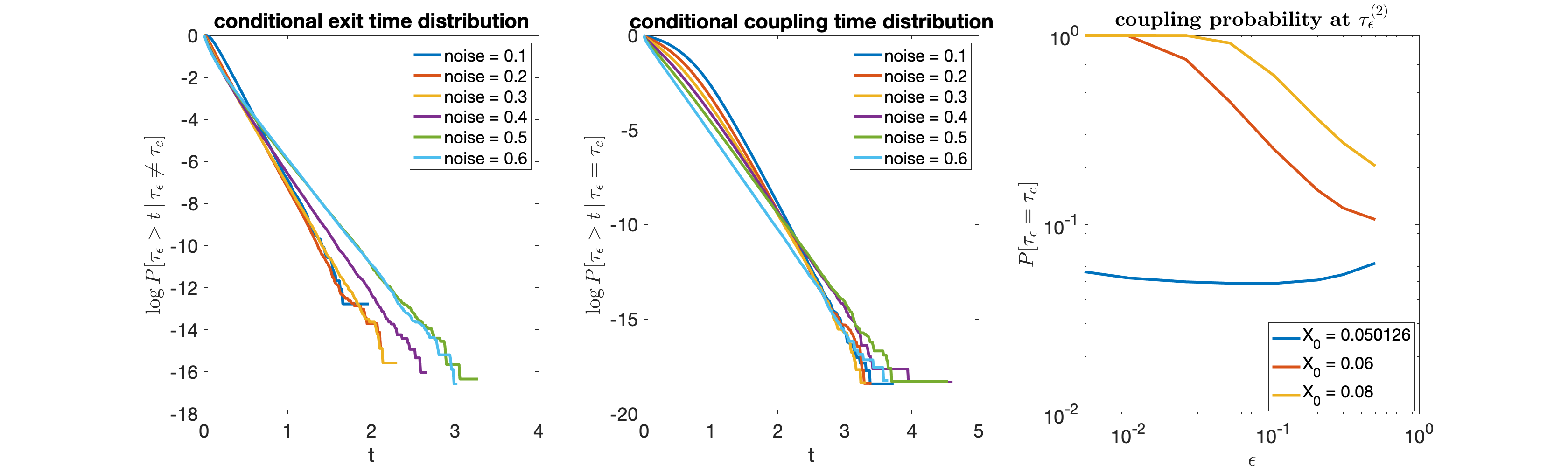
Figure 4. Left: Conditional exit time distribution. Middle: Conditional coupling time distribution. Right: Probability of couple at $\tau_{\varepsilon}$

5.4. Interacting particle system in the double-well potential

In this section, we study a variance of the double well potential of the previous section. Denote

$$V(x)=x^{4}-2x^{2}+0.2x,\quad x\in\mathbb{R}$$

be the double-well potential as in the previous section, and let three particles move along $V$ under the over-damped Langevin dynamics. Assume, besides the potential $V$, there is also a pairwise interaction potential between the three particles. The energy potential for the interacting particle system is

$$U(x_{1},x_{2},x_{3})=\sum\nolimits_{i=1}^{3}V(x_{i})+\sigma\sum\nolimits_{i,j=1,2,3,\,i\neq j}(x_{i}-x_{j})^{2}\,.$$

where $\sigma>0$ is the interaction strength.

It is not hard to see that $U$ has two trivial local minima $x_{1}=x_{2}=x_{3}=0.9740$ and $x_{1}=x_{2}=x_{3}=-1.0241,$ respectively, corresponding to which all the three particles are lying at the same local minimum of $V(x)$. When $\sigma>0$ is sufficiently small, there are another six local minima under which the three particles are staying in the different basins of $V(x)$; see Figure 5 Top for a sample trajectory of the solution of (2).

We see that there are two extreme cases in terms of the interactions of the interacting particle system. One extreme case is when there are no interactions between the three particles, i.e., $\sigma=0.$ In this case, the three particles are independent and passing between the two wells one by one, resulting the same barrier heights with that of the double-well potential $V$. The other extreme case corresponds to $\sigma=\infty$, which means that the interactions between the three particles are so strong that they always have to move together. In this case, the energy potential $U$ has the same local minima as that of $V$ and the essential barrier height is the triple of that of $V$. Hence, the essential barrier height $H_{U}$ of the interacting particle system should lie between that of the two extreme cases, i.e., $0.8076$ and $3\times 0.8076=2.4228$, respectively, and $H_{U}$ increases as $\sigma$ increases.

The distribution of the coupling time $\tau_{c}$ is computed for $\varepsilon=0.4,$ $0.41,$ $0.42,$ $0.43,$ $0.45,$ $0.47,$ $0.5,$ $0.55,$ $0.6,$ and $0.7$ when $\sigma=0.05$, and $\varepsilon=0.41,$ $0.42,$ $0.43,$ $0.44,$ $0.45,$ $0.47,$ $0.5,$ $0.55,$ $0.6$ and $0.7$ when $\sigma=0.1$, and the negative slopes $r(\varepsilon)$ are estimated for both cases. A similar relation of $r(\varepsilon)$ v.s. $\varepsilon$ is observed with the double-well potential, and a linear extrapolation of $-\varepsilon^{2}\log r(\varepsilon)$ provides an estimation of the the essential barrier height. In Figure 5 Middle right, the linear extrapolation yields $r(0)=1.7374$ for $\sigma=0.05$ and $r(0)=1.9598$ for $\sigma=0.1$, both of which are approximately equal to the double of the barrier height $2H_{U}$. As expected, the barrier height increases as the interaction between particles becomes stronger.

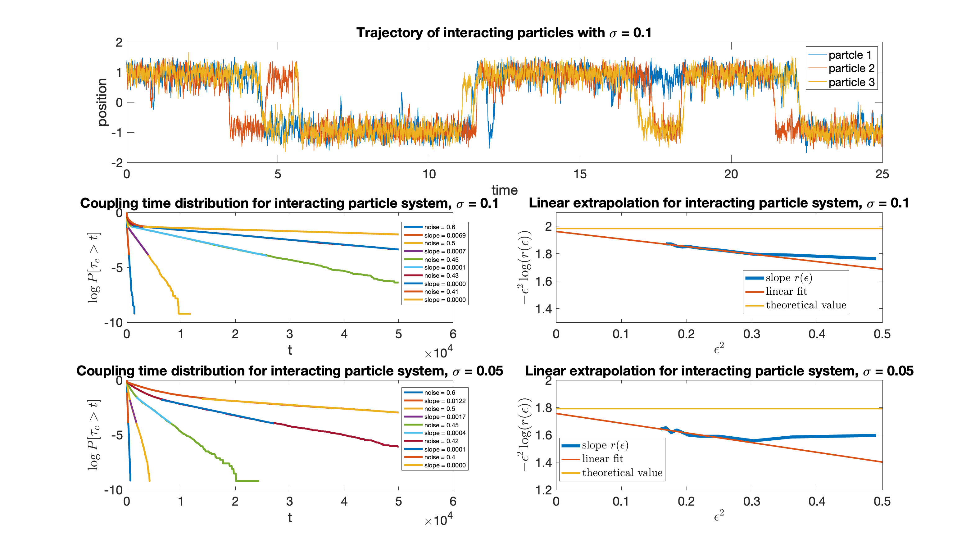
Figure 5. Top: Sample trajectory of a 3-particle interacting particle system in a double well potential. Middle: coupling time distribution and $\varepsilon$ v.s. $-\varepsilon^{2}\log r(\varepsilon)$ with $\sigma=0.05$. Bottom: coupling time distribution and $\varepsilon^{2}$ v.s. $-\varepsilon^{2}\log r(\varepsilon)$ with $\sigma=0.1$. Theoretical values of $r(0)$ are given by the minimum energy path.

The next task is to numerically verify (H1)-(H3) in Section 4 for the setting of multi-well potentials. In the following, the interaction strength is always set as $\sigma=0.05$.

Numerical verification of (H1). Let ${\mathcal{X}}_{0}=(1,1,1),$ and ${\mathcal{Y}}_{0}=(-1,-1,-1)$ so that ${\mathcal{Y}}_{t}$ starts near the global minimum. According to the definition of $\mathcal{I}$ and $\mathcal{J}$, it is easy to see from height of barriers in Figure 8 that $\mathbf{B}_{1}$ is in fact the complement of the basin of attraction that contains $(1,1,1)$. Our simulation uses four noise magnitudes $\varepsilon=0.6,0.65,0.7,$ and $0.75$. After each step of the Euler-Maruyama scheme, it will be numerically checked to determine whether ${\mathcal{X}}_{t}$ and ${\mathcal{Y}}_{t}$ are in $\mathbf{B}_{1}$. Interestingly, we have never seen ${\mathcal{Y}}_{t}$ leaves $\mathbf{B}_{1}$ before ${\mathcal{X}}_{t}$ enters $\mathbf{B}_{1}$ after tens of millions of samples collected. The same thing happens for the 1D double well potential: numerically ${\mathcal{Y}}_{t}$ never leaves $\mathbf{B}_{1}$ before ${\mathcal{X}}_{t}$ enters $\mathbf{B}_{1}$. Hence, (H1) is numerically concluded with a even stronger result that

$$\mathbb{P}\big{[}{\mathcal{Y}}_{s}\in\mathbf{B}_{1}\ \text{for all}\ s\in[0,t]\big{|}\kappa_{\{{\mathcal{X}}_{t}\}}(\mathbf{B}_{1})>t\big{]}\approx 1.$$

Numerical verification of (H2). Let ${\mathcal{X}}_{t}$ and ${\mathcal{Y}}_{t}$ both start from $B_{1}$. We simulate the coupling process until either that ${\mathcal{X}}_{t}$ and ${\mathcal{Y}}_{t}$ are coupled successfully before any one of them exists $B_{1},$ or one of them, ${\mathcal{X}}_{t}$ or ${\mathcal{Y}}_{t},$ exits $B_{1}$ before they are coupled within $B_{1}$, respectively. In Figure 6 Left and Middle panel, the conditional exit time distribution and conditional coupling time distribution are demonstrated, respectively. We see that the slopes of both the two tail distributions are largely unchanged as the noise magnitude decrease from $0.5$ to $0.1$. This is consistent with the result for the double-well potential.

In Figure 6 Right, the coupling probability is demonstrated in term of noise magnitude. Again, similar to the case of double-well potential, when starting within the same basin, the probability $\mathbb{P}[\tau_{\varepsilon}=\tau_{c}]$ significantly increases with respect to a decreasing $\varepsilon$ as the chance of ${\mathcal{X}}_{t},{\mathcal{Y}}_{t}$ to escape from the basin becomes lower. However, for those successfully leave $B_{1}$ before being coupled, the exit time distribution does not change much with respect to the noise magnitudes.

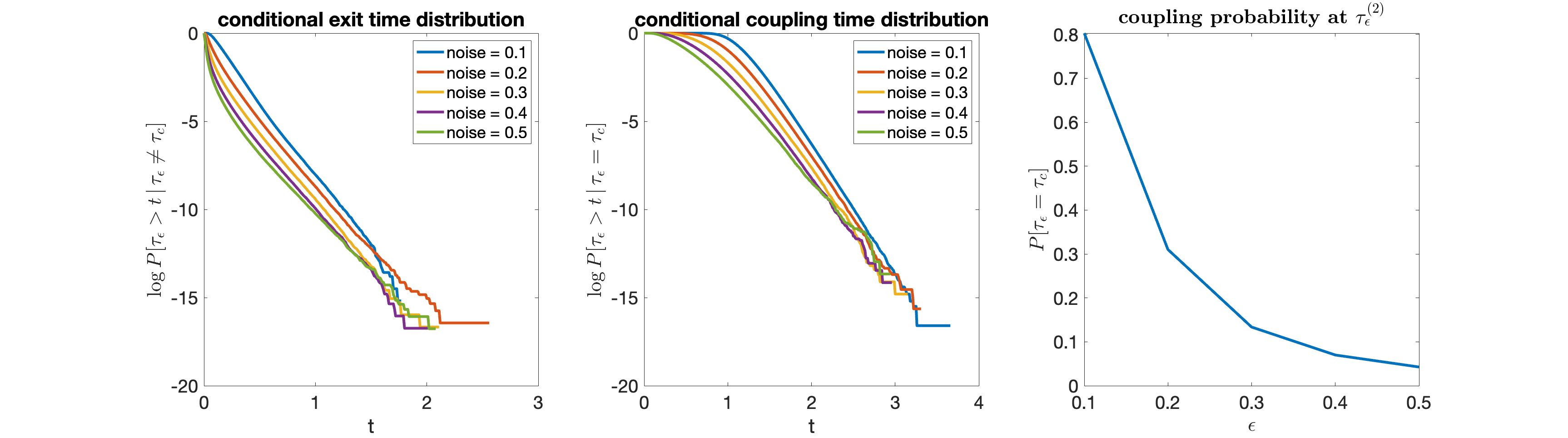
Figure 6. Left: Conditional exit time distribution. Middle: Conditional coupling time distribution. Right: Probability of coupling at $\tau_{\varepsilon}$

Numerical verification of (H3). The (H3) is numerically verified by computing the overshoot time. The criterion of deciding whether a trajectory hits the basin $B_{1}$ is the same as above. The probability distribution of the overshoot time $\xi_{1}-\max\{\kappa_{\mathcal{X}_{t}},\kappa_{\mathcal{Y}_{t}}\}$, i.e., the infimum time when both ${\mathcal{X}}_{t}$ and ${\mathcal{Y}}_{t}$ are staying in $B_{1}$ after each of them has visited $B_{1}$ is computed. The magnitudes of noise are chosen as $0.5,0.55,$ and $0.6$, and for each case, the probability distribution of $\xi_{1}-\max\{\kappa_{\mathcal{X}_{t}},\kappa_{\mathcal{Y}_{t}}\}$ is computed by running $1\times 10^{7}$ samples. As shown in Figure 7, the tail of $\xi_{1}-\max\{\kappa_{\mathcal{X}_{t}},\kappa_{\mathcal{Y}_{t}}\}$ has two phases. The second phase has a slower decrease of the exponential tail but is still faster than that of the coupling time. The second phase comes from the event that one of the two trajectories, $\mathcal{X}_{t}$ or $\mathcal{Y}_{t}$, takes an excursion to other basins after visiting $B_{1}$ and then returns back, while the other trajectory has always been staying in $B_{1}$. Note that the probability of such event is low and a large number of samples are required to capture the exponential tail. In Figure 7, the distributions of the overshoot time and coupling time are compared. We see that the slope of tail distribution of the overshoot time decays quickly as noise vanishes, but still remains steeper than that of the coupling time in the log-linear plot. Since it has been numerically verified that the coupling time distribution is consistent with the theoretical barrier height $H_{U}$, (H3) is verified automatically.

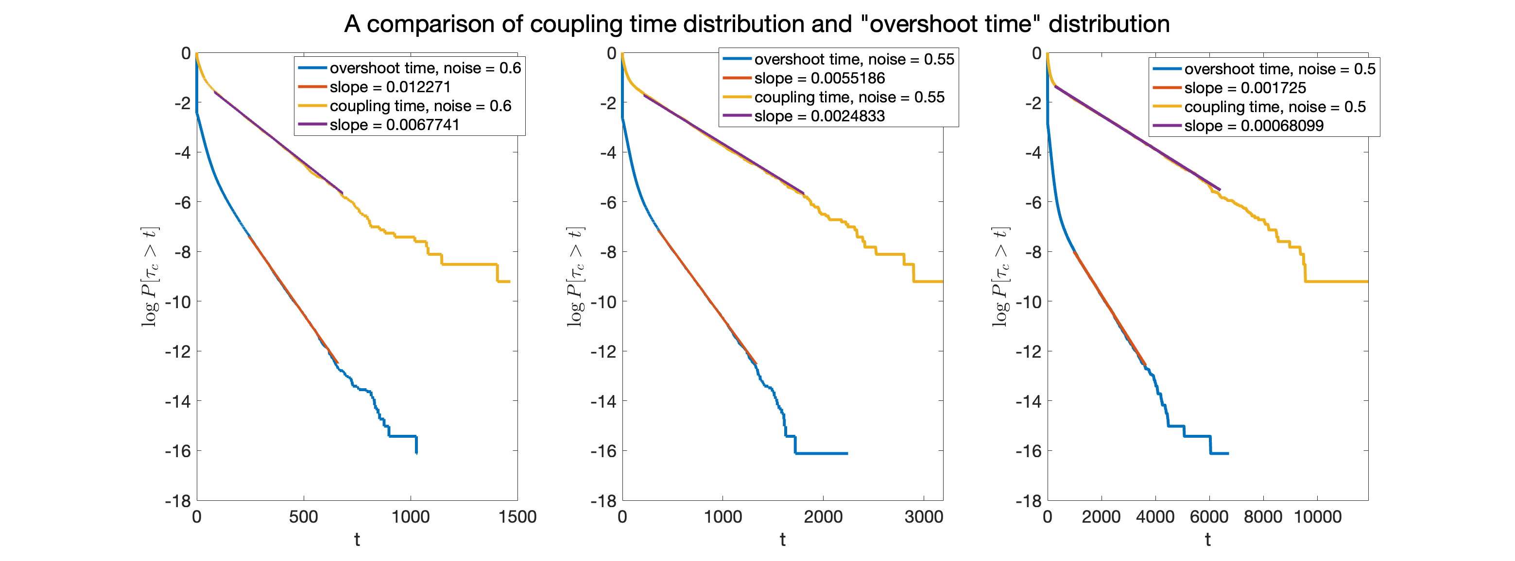
Figure 7. Comparison of probability distributions of the “overshoot time” $\xi_{1}-\max\{\kappa_{\mathcal{X}_{t}},\kappa_{\mathcal{Y}_{t}}\}$ and the coupling time. Left, middle, and right panels are for $\varepsilon=0.6,0.55$, and $0.5$ respectively.

Finally, the String method [12] is used to compute the heights of various barriers between the local minima $(0.9740,0.9740,0.9740)$ and $(-1.0241,-1.0241,-1.0241)$ in the energy landscape to validate the essential barrier height inferred from our coupling approach. As shown in Figure 8, the essential barrier, which is the highest barrier that a trajectory needs to overcome to enter the basin of the global minimum, is leftmost barrier in the lower left panel of Figure 8 (A)(B). In this example, since the three particles are indistinct, the energy potential is rather symmetric for which the eight local minima are of only two types consists of four particular cases that all the three particles are lying in the same well (global or local), or two of the three particles are lying in one well (global or local) with the other particle lying in the other well. We see in Figure 8 that the minimal energy path(MEP) connecting the two minima $(0.9740,0.9740,0.9740)$ and $(-1.0241,-1.0241,-1.0241)$ has actually passed all the four cases. Hence, the essential barrier height $H_{U}$ can be attained by such an MEP although in principle, it has to be taken over all the paths connecting any of the local minima to the global one. In Figure 8, it shows that $H_{U}=0.8961$ for $\sigma=0.05$ and $H_{U}=0.9916$ for $\sigma=0.1$, corresponding to the theoretical value $r(0)=1.7922$ for $\sigma=0.05$ and $r(0)=1.9832$ for $\sigma=0.1,$ respectively.

The result from the String method is further confirmed through the equivalent characterization (23) by numerically solving all the $27$ critical points (including all the local minima and saddle points) of $U$. The essential barrier height obtained in this way is $H_{U}=0.8962$ for $\sigma=0.05$ and $H_{U}=0.9916$ for $\sigma=0.1$, which are almost the same with the essential barrier heights given by the String method. As shown in Figure 5, both values are very close to $r(0)/2$ in the linear extrapolation.

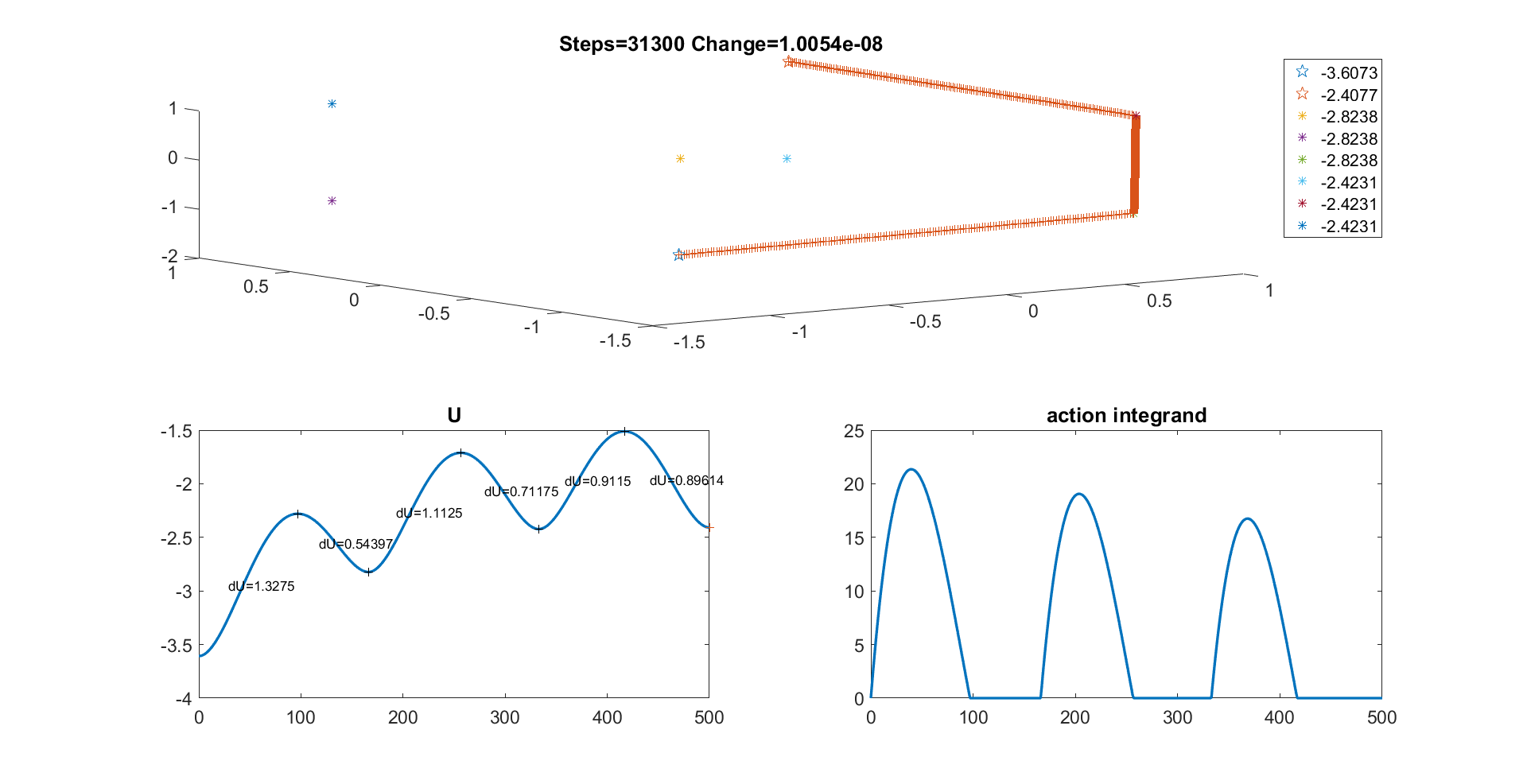
(a) $\sigma=0.05$

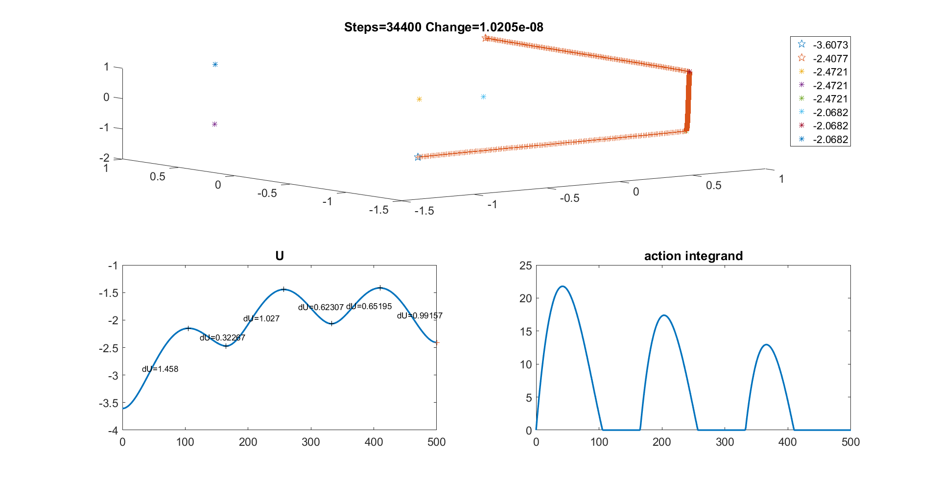
(b) $\sigma=0.1$

Figure 8. Minimum Energy Path (MEP) computed by String method [12] at high numerical resolution. MEP is the mostly likely path for transition from one metastable state to another in the zero-temperature limit of overdamped Langevin, and it is known (e.g., [11]) to reveal barrier heights and descent depths along the transition path, which are labeled by dV values in the bottom left panel. Top panel visualizes the MEP in 3D (i.e., $x_{1},x_{2},x_{3}$) where legend lists the potential $U$’s value at each local minimum. Bottom right panel is the integrand of the Freidlin-Wentzell action functional plotted as a function of arc-length parameterization of the path, which serves as a sanity check to ensure the MEP is computed correctly.

5.5. Rosenbrock function

In this example, we test on the famous non-convex landscape of the Rosenbrock function in 2D and 4D, respectively. For $N\in\mathbb{N}_{+}$, the Rosenbrock function is defined as

$$R_{N}(\bm{x})=\sum_{i=1}^{N-1}[b(x_{i+1}-x_{i}^{2})^{2}+(a-x_{i})^{2}],\quad\bm{x}\in\mathbb{R}^{N},$$

where $a,b$ are two constants. In this example, we choose $a=1,b=20$. When $N=2$, $R_{N}$ has a unique minimum at $(1,1)$, and when $N=4$, $R_{N}$ admits a global minimum $(1,1,1,1)$ and a local minimum $(-1,1,1,1)$. In Figure 9, the landscape of $\log R_{2}(\bm{x})$ is demonstrated in the Top Left panel and a slice of $\log R_{4}(\bm{x})$ at $x_{3}=x_{4}=1$ is demonstrated in the Bottom Left panel. We note that the logarithm scale is used to visualize the detailed landscape near each minimum. We see that near each minimum, the landscape looks like a valley which is only convex on a very small area around the minimum. The landscape of $R_{4}$ cannot be completely visualized by the heat map at a slice. However, it is not hard to check that for $a=1,b=20$, the region on which $R_{4}$ being convex is very small.

In the test of the landscape of $R_{2},$ the noise magnitude is set to be $\varepsilon=0.001,$ $0.01,$ $0.1,$ $1.0,$ $1.5,$ and $2.0$, and $\varepsilon=0.001,$ $0.003,$ $0.01,$ $0.03,$ $0.1,$ $0.3,$ and $1.0$ for $R_{4}$. The coupling time distributions are given in the two right panels of Figure 9. We see that when the noise is sufficiently small, the tail distributions of coupling times are parallel in the log-linear plot since the coupling time is almost determined by the convexity of the convex area near the global minimum. This is consistent with the result of Theorem 1.1. However, as noise magnitude increases, the probability of the coupling process to couple in the entire valley instead of just the vicinity of the global minimum becomes larger, and this changes the tail of the coupling time distributions.

Another interesting phenomenon is that unlike the case of double-well potential, for the potential function $R_{4}$, exponentially small tails of the coupling time distribution with respect to the noise magnitude is not observed even when the noise is as small as $0.001$. Even if one of the coupled processes start at the local minimum $(-1,1,1,1)$, the tail of the coupling time distribution has very little change; see the plot with legend “noise $=0.001$ fixed”. This is because the basin of the local minimum is so shallow with such a low barrier that the stochastic trajectories can easily pass the barrier and enter the valley of the global minimum.

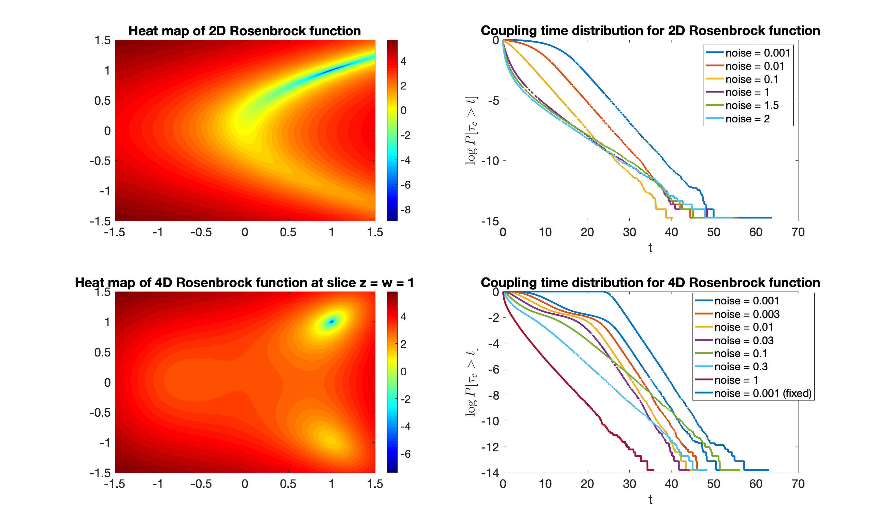
Figure 9. Top Left: landscape of $R_{2}(\bm{x})$. Top Right: Coupling time distribution for $R_{2}(\bm{x})$. Bottom Left: landscape of $R_{4}(\bm{x})$. Bottom Right: Coupling time distribution for $R_{4}(\bm{x})$.

5.6. Loss functions of artificial neural networks

In the last example, the performance of the coupling method in high dimension is examined. We consider the training process of an artificial neural network(ANN) including two hidden layers with $N_{1},N_{2}$ neurons, respectively, which has the following form

$$\mathbf{h}_{1}=\mbox{ReLU}(W_{1}\bm{x}+\mathbf{b}_{1})$$ (67)

$$\mathbf{h}_{2}=\mbox{ReLU}(W_{2}\mathbf{h}_{1}+\mathbf{b}_{2})$$ (68)

$$y=W_{3}\mathbf{h}_{2}+b_{3}\,,$$ (69)

where $\bm{x}\in\mathbb{R}^{2},y\in\mathbb{R},\mathbf{b}_{1}\in\mathbb{R}^{N_{1}},\mathbf{b}_{2}\in\mathbb{R}^{N_{2}},b_{3}\in\mathbb{R}$, and $W_{1}$, $W_{2}$, $W_{3}$ are $N_{1}\times 2$, $N_{2}\times N_{1}$, $1\times N_{2}$ matrices, respectively. Let $\bm{\theta}$ collect the entries of $W_{1},W_{2},W_{3},\mathbf{b}_{1},\mathbf{b}_{2}$, and $b_{3}$ which are the unknown parameters to be determined in the training. Note that the dimension of $\bm{\theta}$ is $(N_{1}N_{2}+3N_{1}+2N_{2}+1)$. For simplicity, (67) - (69) are collectively written as $y=\mbox{NN}(\bm{\theta},\bm{x}).$

For a given training set $\{\bm{x}_{1},\cdots,\bm{x}_{M};y_{1},\cdots y_{M}\}$, let the loss function

$$L(\bm{\theta})=\sum\nolimits_{i=1}^{M}\left(y_{i}-\mbox{NN}(\bm{\theta},\bm{x}_{i})\right)^{2},$$

where the size of the training set $M=100$. The collocation points $\bm{x}_{1},\cdots,\bm{x}_{100}$ are uniformed sampled from $[-1\,,1]^{2}$, $y_{i}=|\bm{x}_{i}|^{2}$; see the first column of Figure 11 for the distribution of collocation points and the target function $y=|\bm{x}|^{2}$. What we are interested in is the landscape of the loss surface $L(\bm{\theta})$.

Our coupling algorithm is tested on three ANNs for which the size of hidden layers are $N_{1}=4,N_{2}=3$, $N_{1}=N_{2}=10$, and $N_{1}=N_{2}=20$, which are called the “small network”, “medium network”, and “big network”, respectively. Note that in this example, the small network is under-parameterized and the big network is over-parameterized. It is believed that over-parametrization lowers the barrier heights of ANNs (e.g., [17, 33, 6, 26, 30, 31, 10]) which, however, is not easy to justify because the loss landscape is usually in high-dimension and very complicated. Our coupling approach provides a feasible way to explore this by computing the essential barrier height of the entire landscape.

In Figure 10, the coupling time distribution of each ANN is computed under $10$ different magnitudes of noise (while only $5$ of them are demonstrated in the figure to avoid a too crowded legend though). Similar to the previous examples, all slopes are estimated through the weighted linear fitting. The six smallest values of $\varepsilon^{2}$ are used in the linear extrapolation of $-\varepsilon^{2}\log r(\varepsilon)$ v.s. $\varepsilon^{2}$ which are demonstrated in the three lower panels. We see that the larger neural network has a lower essential barrier height. This is consistent with the study in [10] in which MEPs are computed between the local minima of loss functions of ANNs.

The small neural network in this example is under-parametrized because the number of unknown parameters to be determined is 31 while the size of the training set is $100$. As shown in Figure 10, the loss function of the small neural network has a much larger essential barrier height than that of both the medium and big neural networks. In the training process, when start from random initial conditions, the small neural network may converge to a “bad” local minimum which does not fit the target function very well (see the middle panels of Figure 11). In contrast, for all the initial values that have been tested, both the medium and big neural networks converge to a “good” local minimum that approximates the target function reasonably well (see the right panels of Figure 11). This is consistent with some known results on the loss surface of artificial neural networks in the literature [7, 20, 32].

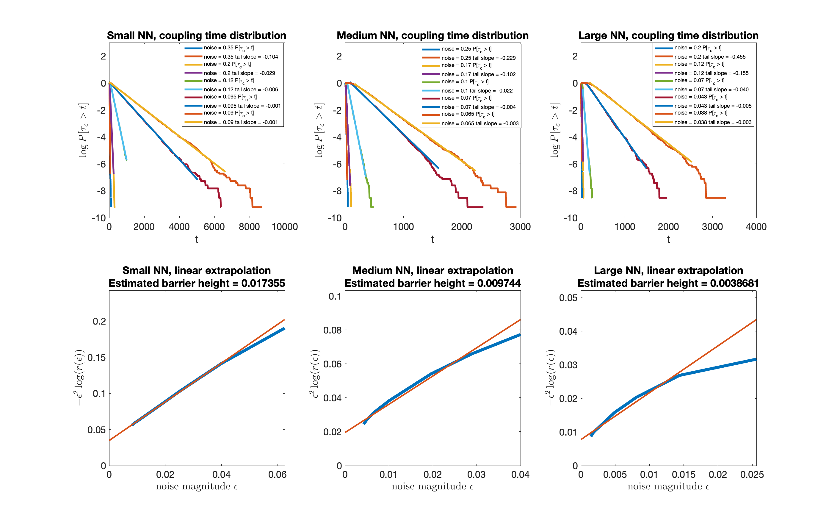
Figure 10. Coupling time distribution and linear extrapolation of $-\varepsilon^{2}\log r(\varepsilon)$ v.s. $\varepsilon^{2}$. Left: small network. Middle: medium network, Right: large network.

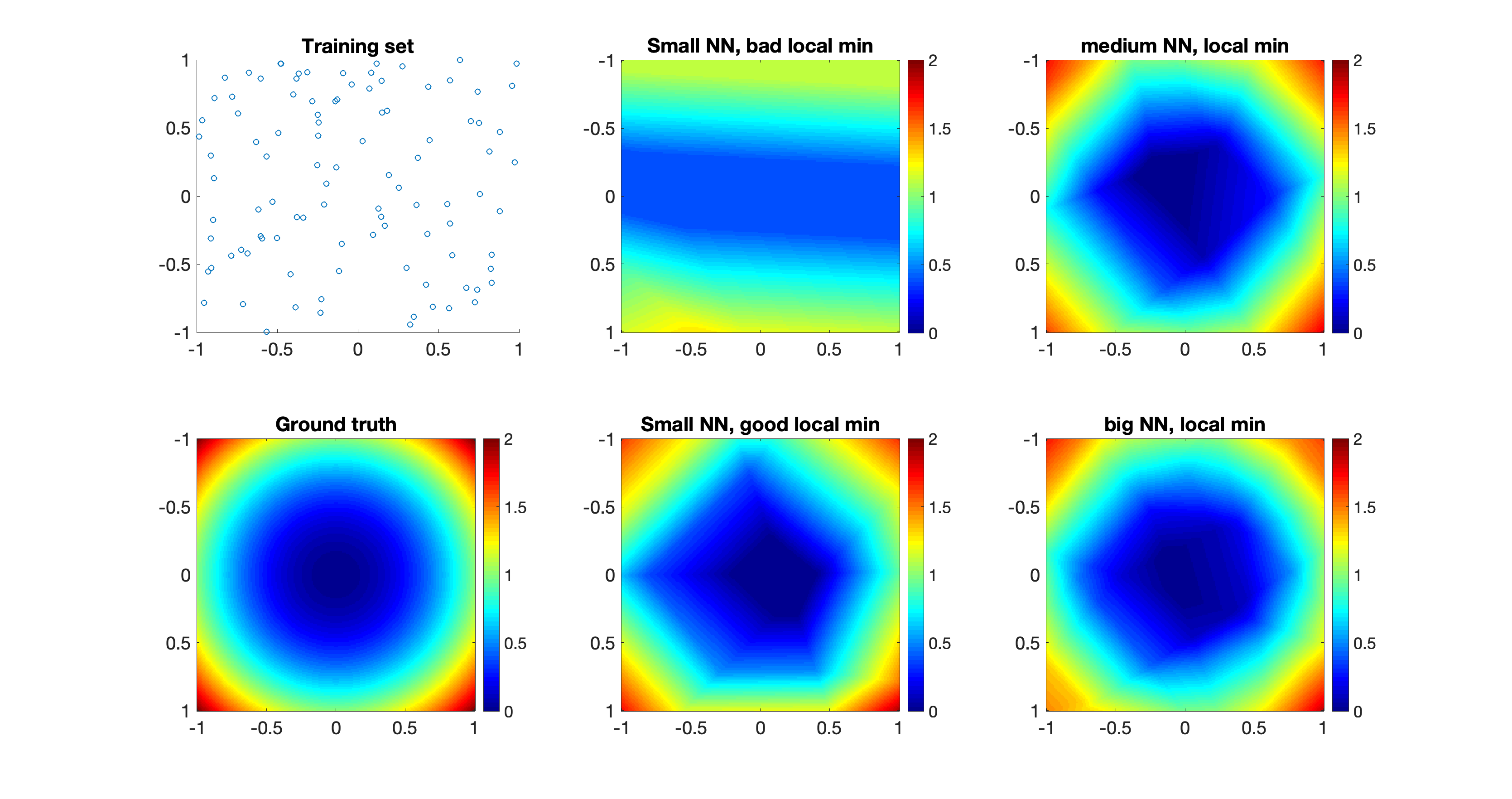
Figure 11. Left column: training set and target function. Middle column: $y=\mbox{NN}(\bm{\theta},\bm{x})$ for $\bm{\theta}$ at bad and good local minima of the small network. Right column: $y=\mbox{NN}(\bm{\theta},\bm{x})$ from medium and big neural network.

6. Conclusion and further discussions

This paper investigates the relations between the landscape of a multi-dimensional potential function and the coupling time distributions of the overdamped Langevin system with respect to the given potential. This is motivated by the fact that the exponential tail of the coupling time distribution gives a lower bound of the spectral gap of the Fokker-Planck operator of the overdamped Langevin dynamics. It has been known for a long time that some global information can be inferred from the spectrum of a differential operator, such as detailed by the famous problem “Can one hear the shape of a drum?” in [18]. As expected, certain connections between the shape of the landscape and the coupling time distributions are established.

This paper shows that as the magnitude of the noise vanishes, the variation of the exponential tails of the distribution of the overdamped Langevin dynamics of a single-well potential differs from that of a multi-well potential in a qualitative way. More specifically, for single-well potential functions that are strongly convex, the exponential tails is bounded from above by a constant depending on the convexity of the potential function; for a multi-well potential function, however, the exponential tail decreases exponentially fast as the noise magnitude goes to zero. A linear extrapolation can then be used to infer the slope of the exponential tail in the vanishing limit of the noise, which is defined and called the essential barrier height, characterizing the barrier height of the potential landscape in the global way. All these claims are justified both theoretically and numerically. In particular, the numerical results for the loss surface of artificial neural networks are corroborated by other studies in certain different ways.

The coupling scheme used in this paper is a combination of two coupling methods, the reflection coupling and maximal coupling, for the purpose of coupling efficiency. We find that the bound provided by the reflection-maximal coupling scheme is reasonably close to the optimal one (i.e., the one that makes the coupling inequality becomes an equality). Although in this paper only the coupling time is examined, more information are expected to be inferred from the coupling result in future work, e.g., the coupling location may provide us additional information about the landscape. In addition, this paper only considers the tail of the coupling time distribution that is related to the principal eigenvalue of the Fokker-Planck operator. The entire coupling time distribution, however, may provide additional information on the non-principal eigenvalue of the Fokker-Planck operator. For example, for a multi-well potential, the conditional coupling time distribution conditioning on not being coupled in the deepest “well” may be related to the heights of lower barriers. These could be potentially interesting future directions.

References

- [1] Alan Agresti and Brent A. Coull, Approximate is better than ’exact’ for interval estimation of binomial proportions, The American Statistician. 52 (1998), no. 2, 119–126.
- [2] David Aldous, Random walks on finite groups and rapidly mixing Markov chains, Séminaire de Probabilités XVII 1981/82, Springer, 1983, pp. 243–297.
- [3] Erich Baur, Metastabilität von reversiblen diffusionsprozessen., Diploma thesis, Bonn University (2011).
- [4] Anton Bovier, Michael Eckhoff, Vèronique Gayrard, and Markus Klein, Metastability in reversible diffusion processes. i. sharp asymptotics for capacities and exit times, J. Eur. Math. Soc. 6 (2004), no. 4, 399––424.
- [5] Anton Bovier, Vèronique Gayrard, and Markus Klein, Metastability in reversible diffusion processes. ii. precise asymptotics for small eigenvalues, J. Eur. Math. Soc. 7 (2005), no. 1, 69––99.
- [6] Lenaic Chizat, Edouard Oyallon, and Francis Bach, On lazy training in differentiable programming, Advances in Neural Information Processing Systems 32 (2019).
- [7] Anna Choromanska, Mikael Henaff, Michael Mathieu, Gérard Ben Arous, and Yann LeCun, The loss surfaces of multilayer networks, Artificial intelligence and statistics, PMLR, 2015, pp. 192–204.
- [8] Martin Day, On the exponential exit law in the small parameter exit problem, Stochastics 8 (1983), no. 4, 297––323.
- [9] Luc Devroye, Mehrabian Abbas, and Reddad Tommy, The total variation distance between high-dimensional gaussians, arXiv:1810.08693 (2018).
- [10] Felix Draxler, Kambis Veschgini, Manfred Salmhofer, and Fred Hamprecht, Essentially no barriers in neural network energy landscape, International conference on machine learning, PMLR, 2018, pp. 1309–1318.
- [11] Weinan E, Weiqing Ren, and Eric Vanden-Eijnden, String method for the study of rare events, Physical Review B 66 (2002), no. 5, 052301.
- [12] by same author, Simplified and improved string method for computing the minimum energy paths in barrier-crossing events, Journal of Chemical Physics 126 (2007), no. 16, 164103.
- [13] Mark Freidlin and Alexander Wentzell, Random Perturbations of Dynamical Systems, Springer, 1998.
- [14] Emmanuel Gobet and Stéphane Menozzi, Exact approximation rate of killed hypoelliptic diffusions using the discrete euler scheme, Stochastic Processes and their Applications 112 (2004), no. 2, 201–223.
- [15] by same author, Stopped diffusion processes: boundary corrections and overshoot, Stochastic Processes and their Applications 120 (2010), no. 2, 130–162.
- [16] Victor Yakovlevich Ivrii, On the second term of the spectral asymptotics for the laplace–beltrami operator on manifolds with boundary and for elliptic operators acting in fiberings, Doklady Akademii Nauk, vol. 250, Russian Academy of Sciences, 1980, pp. 1300–1302.
- [17] Arthur Jacot, Franck Gabriel, and Clément Hongler, Neural tangent kernel: Convergence and generalization in neural networks, Advances in neural information processing systems 31 (2018).
- [18] Mark Kac, Can one hear the shape of a drum?, Amer. Math. Monthly 73 (2020), no. 4 Part II, 1–23.
- [19] Stuart Kauffman and Simon Levin, Towards a general theory of adaptive walks on rugged landscapes, J. Theor. Biol. 128 (1987), no. 1, 11–45.
- [20] Kenji Kawaguchi, Jiaoyang Huang, and Leslie Pack Kaelbling, Every local minimum value is the global minimum value of induced model in nonconvex machine learning, Neural Computation 31 (2019), no. 12, 2293–2323.
- [21] Paul Krugman, Complex landscapes in economic geography, Am. Econ. Rev. 84 (1994), no. 2, 412–416.
- [22] Boris Leblanc, Renault Olivier, and Olivier Scaillet, A correction note on the first passage time of an ornstein-uhlenbeck process to a boundary, Finance Stoch. 4 (2000), no. 1, 109–111.
- [23] Yao Li and Shirou Wang, Numerical computations of geometric ergodicity for stochastic dynamics, Nonlinearity 33 (2020), no. 12, 6935–6970.
- [24] Torgny Lindvall, Lectures on the coupling method, Courier Corporation, 2002.
- [25] Torgny Lindvall and L. C. G Rogers, Coupling of multidimensional diffusions by reflection, Ann. Probab. 14 (1986), no. 3, 860––872.
- [26] Song Mei, Theodor Misiakiewicz, and Andrea Montanari, Mean-field theory of two-layers neural networks: dimension-free bounds and kernel limit, Conference on Learning Theory, PMLR, 2019, pp. 2388–2464.
- [27] Morris Newman and John Todd, The evaluation of matrix inversion programs, J. Soc. Indust. Appl. Math. 6 (1958), 466––476.
- [28] Esa Nummelin and Pekka Tuominen, Geometric ergodicity of harris recurrent markov chains with applications to renewal theory, Stochastic Process. Appl. 12 (1982), no. 2, 187––202.
- [29] Gilles Pagès and Fabien Panloup, Unajusted langevin algorithm with multiplicative noise: Total variation and wasserstein bounds, arXiv:2012.14310 (2020).
- [30] Grant M Rotskoff and Eric Vanden-Eijnden, Trainability and accuracy of neural networks: An interacting particle system approach, arXiv preprint arXiv:1805.00915 (2018).
- [31] Justin Sirignano and Konstantinos Spiliopoulos, Mean field analysis of neural networks: A central limit theorem, Stochastic Processes and their Applications 130 (2020), no. 3, 1820–1852.
- [32] Mahdi Soltanolkotabi, Adel Javanmard, and Jason D Lee, Theoretical insights into the optimization landscape of over-parameterized shallow neural networks, IEEE Transactions on Information Theory 65 (2018), no. 2, 742–769.
- [33] Mei Song, Andrea Montanari, and P Nguyen, A mean field view of the landscape of two-layers neural networks, Proceedings of the National Academy of Sciences 115 (2018), no. 33, E7665–E7671.
- [34] David Wales, Energy landscapes: Applications to clusters, biomolecules and glasses, Cambridge University Press, 2003.
- [35] Hermann Weyl, Über die asymptotische verteilung der eigenwerte, Nachrichten von der Gesellschaft der Wissenschaften zu Göttingen, Mathematisch-Physikalische Klasse 1911 (1911), 110–117.
- [36] Steve Zelditch, Spectral determination of analytic bi-axisymmetric plane domains, Geometric & Functional Analysis GAFA 10 (2000), no. 3, 628–677.