Binary black hole spins: model selection with GWTC-3

Abstract

The origin of the spins of stellar-mass black holes is still controversial, and angular momentum transport inside massive stars is one of the main sources of uncertainty. Here, we apply hierarchical Bayesian inference to derive constraints on spin models from the 59 most confident binary black hole merger events in the third gravitational-wave transient catalogue (GWTC-3). We consider up to five parameters: chirp mass, mass ratio, redshift, effective spin, and precessing spin. For model selection, we use a set of binary population synthesis simulations spanning drastically different assumptions for black hole spins and natal kicks. In particular, our spin models range from maximal to minimal efficiency of angular momentum transport in stars. We find that, if we include the precessing spin parameter into our analysis, models predicting only vanishingly small spins are in tension with GWTC-3 data. On the other hand, models in which most spins are vanishingly small, but that also include a sub-population of tidally spun-up black holes are a good match to the data. Our results show that the precessing spin parameter has a crucial impact on model selection.

1 Introduction

The third observing run (O3) of the Advanced LIGO (Aasi et al., 2015) and Virgo (Acernese et al., 2015) detectors has brought the number of compact binary merger observations up to 90 events with a probability of astrophysical origin $>0.5$ (Abbott et al., 2019, 2021d, 2021a, 2021b). In particular, the 63 confident detections of binary black hole (BBH) mergers (with a false alarm rate FAR$<0.25$ yr^-1) lead to more accurate constraints on the mass and spin distribution of these systems (Abbott et al., 2021c).

The intrinsic distribution of primary black hole (BH) masses inferred by the LIGO–Virgo–KAGRA collaboration (hereafter, LVK) shows several sub-structures, including a main peak at $\approx{10}$ M_⊙, a secondary peak at $\approx{30-40}$ M_⊙, and a long tail extending up to $\sim{80}$ M_⊙ (e.g., Abbott et al., 2021c). The inferred distribution of mass ratios has a strong preference for equal-mass systems, but several BBHs are confidently unequal-mass (e.g.,GW190412 Abbott et al., 2020)(,GW190517 Abbott et al., 2021d). Focusing on BH spins, we can safely exclude that all BHs are maximally spinning (Farr et al., 2017; Farr et al., 2018; Abbott et al., 2019). Typical spin magnitudes in BBHs are small, with $\sim{50}$% of BHs having $\chi\lesssim{}0.3$ (e.g., Wysocki et al., 2019; Abbott et al., 2021d), although not all BHs in the LVK sample have zero spin (Roulet & Zaldarriaga, 2019; Miller et al., 2020). For example, GW151226 (Abbott et al., 2016a) and GW190517 (Abbott et al., 2021c) confidently possess spin. LVK data also support some mild evidence for spin-orbit misalignment (e.g., Tiwari et al., 2018; Abbott et al., 2021d, c; Venumadhav et al., 2020; Olsen et al., 2022; Callister et al., 2021; Hannam et al., 2022; Callister et al., 2022).

These results provide crucial insights to understand BBH formation and evolution (e.g., Gerosa et al., 2013; Stevenson et al., 2015; Rodriguez et al., 2016; Stevenson et al., 2017; Talbot & Thrane, 2017; Fishbach & Holz, 2017; Vitale et al., 2017; Zevin et al., 2017; Farr et al., 2018; Barrett et al., 2018; Taylor & Gerosa, 2018; Fragione & Kocsis, 2020; Arca Sedda & Benacquista, 2019; Roulet & Zaldarriaga, 2019; Wysocki et al., 2019; Bouffanais et al., 2019, 2021a, 2021b; Kimball et al., 2021; Kimball et al., 2020; Baibhav et al., 2020; Arca Sedda et al., 2020; Zevin et al., 2021; Mapelli et al., 2021; Mapelli et al., 2022). Moreover, the mass and spin of BHs carry the memory of their progenitor stars and therefore are a key to unravel the details of massive star evolution and collapse (e.g., Fryer & Kalogera, 2001; Heger et al., 2003; Belczynski et al., 2010; Mapelli et al., 2013; Fragos & McClintock, 2015; Marchant et al., 2016; Eldridge & Stanway, 2016; de Mink & Mandel, 2016; Spera & Mapelli, 2017; Bavera et al., 2020; Belczynski et al., 2020; Fragione et al., 2022; Mandel et al., 2021; Fryer et al., 2022; Olejak et al., 2022; Chattopadhyay et al., 2022; van Son et al., 2022; Briel et al., 2022; Stevenson & Clarke, 2022; Broekgaarden et al., 2022a; Broekgaarden et al., 2022b). In particular, the spin magnitude of a stellar-origin BH should retain the imprint of the spin of the core of its progenitor star (e.g., Qin et al., 2018; Qin et al., 2019; Fuller & Ma, 2019; Bavera et al., 2020; Belczynski et al., 2020; Olejak & Belczynski, 2021; Stevenson, 2022).

Several models have been proposed to infer the spin magnitude of the BH from that of the progenitor star. The main open question concerns the efficiency of angular momentum transport within a star (e.g., Maeder & Meynet, 2000; Cantiello et al., 2014; Fuller et al., 2019). If angular momentum is efficiently transferred from the core to the outer layers, mass loss by stellar winds can dissipate most of it, leading to a low-spinning stellar core and then to a low-spinning BH. If instead the core retains most of its initial angular momentum until the final collapse, the BH will be fast spinning.

In the shellular model (Zahn, 1992; Ekström et al., 2012; Limongi & Chieffi, 2018; Costa et al., 2019), angular momentum is mainly transported by meridional currents and shear instabilities, leading to relatively inefficient spin dissipation. In contrast, according to the Tayler-Spruit dynamo mechanism (Spruit, 2002), differential rotation induces the formation of an unstable magnetic field configuration, leading to an efficient transport of angular momentum via magnetic torques. Building upon the Tayler-Spruit mechanism, Fuller & Ma (2019) derived a new model with an even more efficient angular momentum dissipation, predicting that the core of a single massive star might end its life with almost no rotation.

Electromagnetic observations yield controversial results. Asteroseismology favours slowly rotating cores in the late evolutionary stages, but the vast majority of stars with an asteroseismic estimate of the spin are low-mass stars (Mosser et al., 2012; Gehan et al., 2018; Aerts et al., 2019). Continuum-fitting derived spins of BHs in high-mass X-ray binaries are extremely high (e.g., Reynolds, 2021; Miller-Jones et al., 2021; Fishbach & Kalogera, 2022), but such measurements might be affected by substantial observational biases (e.g., Reynolds, 2021). Finally, BH spins inferred from quasi periodic oscillations yield notably smaller values than continuum fitting. For example, the estimate of the dimensionless spin of the BH in GRO J1655–40 is $\chi=0.7\pm{}0.1$ and $0.290\pm{}0.003$ from continuum fitting (Shafee et al., 2006) and quasi-periodic oscillations (Motta et al., 2014), respectively.

In a binary system, the evolution of the spin is further affected by tidal forces and accretion, which tend to spin up a massive star, whereas non-conservative mass transfer and common-envelope ejection enhance mass loss, leading to more efficient spin dissipation (Kushnir et al., 2016; Hotokezaka & Piran, 2017; Zaldarriaga et al., 2018; Qin et al., 2018). For example, the model by Bavera et al. (2020) shows that the second-born BH can be highly spinning if its progenitor was tidally spin up when it was a Wolf-Rayet star orbiting about the first-born BH.

Furthermore, the orientation of the BH spin with respect to the orbital angular momentum of the binary system encodes information about binary evolution processes. In a tight binary system, tides and mass transfer tend to align the stellar spins with the orbital angular momentum (Gerosa et al. 2018, but see Stegmann & Antonini 2021 for a possible spin flip process induced by mass transfer). If the binary system is in the field, the supernova kick is the main mechanism that can misalign the spin of a compact object with respect to the orbital angular momentum, by tilting the orbital plane (e.g., Kalogera, 2000). Finally, the spins of BHs in dynamically formed binary systems are expected to be isotropically distributed, because close encounters in a dense stellar cluster reset any previous signature of alignment (e.g., Rodriguez et al., 2016; Mapelli et al., 2021).

Here, we perform a model-selection hierarchical Bayesian analysis on confident LVK BBHs ($p_{\rm astro}\,>\,0.9$ and $\mathrm{FAR}\,<\,0.25\,{\rm yr}^{-1}$). We consider models of field BBHs for three of the most used angular-momentum transport models: (i) the shellular model as implemented in the Geneva stellar evolution code (Ekström et al., 2012), (ii) the Tayler-Spruit dynamo model as implemented in the mesa code (Cantiello et al., 2014), and (iii) the model by Fuller & Ma (2019). Hereafter, we will refer to these three models simply as GENEVA (G), MESA (M) and FULLER (F) models, following the description in Belczynski et al. (2020).

For each of these models, we consider an additional variation accounting for the Wolf-Rayet (WR) star tidal spin-up mechanism described by Bavera et al. (2020). Also, we account for spin tilts induced by core-collapse supernova explosions.

This paper is organized as follows. Section 2 presents our population-synthesis models. Section 3 describes the hierarchical Bayesian framework we used and discusses the LVK events used in our study. We lay down the results in Section 4, and summarize our conclusions in Section 5.

2 Astrophysical Models

2.1 mobse and natal kicks

We simulated our binary systems with the code mobse (Mapelli et al., 2017; Giacobbo et al., 2018). mobse is a custom and upgraded version of bse (Hurley et al., 2000, 2002), in which we introduced metallicity-dependent stellar winds for OB (Vink et al., 2001), WR (Belczynski et al., 2010), and luminous blue variable stars (Giacobbo & Mapelli, 2018). mobse includes a formalism for electron-capture (Giacobbo & Mapelli, 2019), core-collapse (Fryer et al., 2012), and (pulsational) pair-instability supernovae (Mapelli et al., 2020). Here, we adopt the rapid core-collapse supernova prescription, which enforces a gap between the maximum mass of neutron stars and the minimum mass of BHs (2–5 M_⊙, Özel et al. 2010; Farr et al. 2011).

We model natal kicks of neutron stars and BHs according to three different models, as shown in Fig. 1:

• A unified kick model, in which both neutron stars and BHs receive a kick $v_{\rm kick}\propto{}m_{\rm ej}/m_{\rm rem}$, where $m_{\rm ej}$ is the mass of the ejecta and $m_{\rm rem}$ the mass of the compact remnant (Giacobbo & Mapelli, 2020, hereafter GM20). This model naturally produces low-kicks for electron-capture, stripped and ultra-stripped supernovae (Tauris et al., 2015; Tauris et al., 2017). Hereafter, we call this model GM20.

• A model in which compact-object kicks are drawn from a Maxwellian curve with one-dimensional root-mean-square $\sigma=265$ km s^-1, consistent with observations of Galactic pulsars (Hobbs et al., 2005). This realistically represents the upper limit for BH natal kicks. Hereafter, we name this model $\sigma{}265$.

• A model in which compact-object kicks are drawn from a Maxwellian curve with $\sigma=150$ km s^-1. This value of $\sigma$ is more similar to what suggested from indirect measurements of Galactic BH kicks (e.g., Repetto et al., 2017; Atri et al., 2019). Hereafter, we refer to this model as $\sigma{}150$.

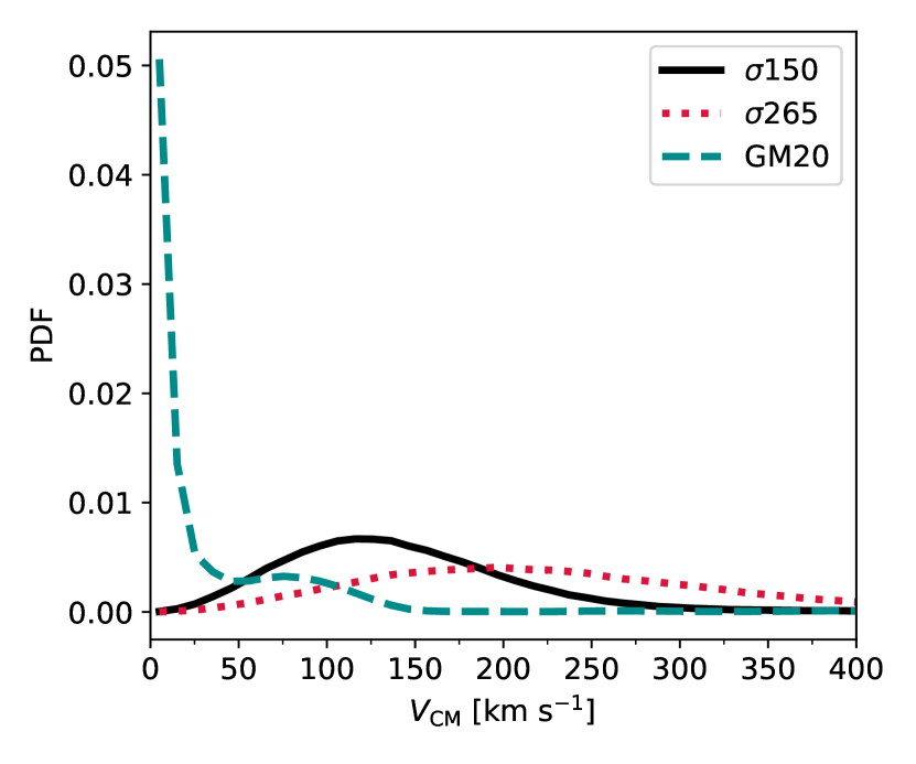
Figure 1: Probability distribution function (PDF) of the binary kick velocities in the centre of mass ($V_{\rm CM}$), for our sample of simulated BBH mergers. The centre-of-mass kick velocity takes into account both the first and the second supernova event in each binary system (Perna et al., 2022). Dashed dark-cyan line: model GM20; solid black line: $\sigma{}150$; dotted red line: $\sigma{}265$. This figure only shows the kick velocity of the stellar progenitors of BBHs that merge within the lifetime of the Universe.

For more details about mobse, see Giacobbo & Mapelli (2018). mobse is an open-source code and can be downloaded from this link.

2.2 Spin magnitude

We have implemented four models for the spin magnitude in mobse, the first three from Belczynski et al. (2020), and the fourth from Bouffanais et al. (2019). Given the large uncertainties on angular momentum transport, we do not claim that these four models are a complete description of the underlying physics: our models must be regarded as toy models, which bracket the current uncertainties on BH spins.

2.2.1 Geneva (G) model

In the Geneva (hereafer, G) model, the dimensionless natal spin magnitude of a BH ($\chi{}$) can be approximated as:

$$\chi{}=\begin{cases}0.85&M_{\textup{CO}}\leq m_{1}\\ a\,{}M_{\textup{CO}}+b&m_{1}<M_{\textup{CO}}<m_{2}\\ a_{\textup{low}}&M_{\textup{CO}},\geq m_{2}\end{cases}$$ (1)

where $a=-0.088$ for all models, $M_{\rm CO}$ is the final carbon-oxygen mass of the progenitor star, while the values of $b$, $m_{1}$, $m_{2}$, and $a_{\rm low}$ depend on metallicity, as indicated in Table 1. This model springs from a fit by Belczynski et al. (2020) to some evolutionary tracks by the Geneva group (Ekström et al., 2012), in which angular momentum transport is relatively inefficient.

$b$	$m_{1}\,{}({\rm M}_{\odot})$	$m_{2}\,{}({\rm M}_{\odot})$	$a_{\rm low}$	$Z$
2.258	16.0	24.2	0.13	$\geq{}0.010$
3.578	31.0	37.8	0.25	$[0.004,\,{}0.010)$
2.434	18.0	27.7	0.0	$[0.0012,0.004)$
3.666	32.0	38.8	0.25	$<0.0012$

Table 1: Parameters adopted in model G. See Eq. 1 for details.

2.2.2 MESA (M) model

In the M model, we use the fits done by Belczynski et al. (2020) to a set of stellar tracks run with the mesa code. mesa models the transport of angular momentum according to the Tayler-Spruit magnetic dynamo (Spruit 2002, see also Cantiello et al. 2014). This yields a dimensionless natal BH spin

$$\chi{}=\begin{cases}a_{1}\,{}M_{\textup{CO}}+b_{1}&{\rm if}\,{}M_{\textup{CO}}\leq m_{1}\\ a_{2}\,{}M_{\textup{CO}}+b_{2}&{\rm if}\,{}M_{\textup{CO}}>m_{1},\end{cases}$$ (2)

where $a_{1}$, $b_{1}$, and $m_{1}$ are given in Table 2.

$a_{1}$	$b_{1}$	$a_{2}$	$b_{2}$	$m_{1}\,{}({\rm M}_{\odot})$	$Z$
$-0.0016$	0.115	–	–	$\infty$	$\geq{}0.010$
$-0.0006$	0.105	–	–	$\infty$	$[0.004,\,{}0.010)$
$0.0076$	0.050	$-0.0019$	0.165	$12.09$	$[0.0012,0.004)$
$-0.0010$	0.125	–	–	$\infty$	$\leq{}0.0012$

Table 2: Parameters adopted in model M. See Eq. 2 for details.

2.2.3 Fuller (F) model

Fuller & Ma (2019) predict that angular momentum transport can be even more efficient than the one predicted by the Tayler-Spruit dynamo. Belczynski et al. (2020) summarize the results of the model by Fuller & Ma (2019) simply as $\chi{}=0.01$ for all single stars and metallicities.

2.2.4 Maxwellian model (Max)

Finally, we also introduce a toy model in which we represent the spin of a BH as a random number drawn from a Maxwellian curve with one-dimensional root-means square $\sigma{}_{\chi}=0.1$ and truncated to $\chi_{\rm max}=1.0$. This model has been first introduced by Bouffanais et al. (2019), because it is a good match to the distribution arising from LVK data (e.g., Abbott et al., 2019, 2021d, 2021c). Hereafter, we will indicate this Maxwellian toy model as Max, for brevity.

2.3 Tidal spin up

The progenitor star of the second-born BH can be substantially spun-up by tidal interactions. In the scenario explored by Bavera et al. (2020), a common-envelope or an efficient stable mass transfer episode can lead to the formation of a BH–WR binary system, in which the WR star is the result of mass stripping. The orbital period of this BH–WR binary system can be sufficiently short to lead to efficient tidal synchronisation and spin-orbit coupling. The WR star is then efficiently spun-up. If the WR star then collapses to a BH directly, the final spin of the BH will retain the imprint of the final WR spin.

Based on the simulations by Bavera et al. (2020), Bavera et al. (2021) derive a fitting formula to describe the spin-up of the WR star and the final spin of the second-born BH:

$$\chi{}=\begin{cases}\alpha_{\rm WR}\log_{10}^{2}{(P/[\textup{day}])}+\beta_{\rm WR}\,{}\log_{10}{(P/\textup{day})}&{\rm if}P\leq 1\,{}\textrm{d}\\ 0&\textrm{otherwise},\end{cases}$$ (3)

where $P$ is the orbital period of the BH–WR sytem, $\alpha_{\rm WR}=f\left(M_{\rm WR},c^{\alpha}_{1},c^{\alpha}_{2},c^{\alpha}_{3}\right)$ and $\beta_{\rm WR}=f\left(M_{WR},c^{\beta}_{1},c^{\beta}_{2},c^{\beta}_{3}\right)$. In this definition,

$$f\left(M_{\rm{WR}},c_{1},c_{2},c_{3}\right)=\frac{-c_{1}}{c_{2}+\exp{\left(-c_{3}M_{\rm{WR}}/[{\rm M}_{\odot}]\right)}},$$ (4)

where $M_{\rm WR}$ is the mass of the WR star, while the coefficients $c_{1}$, $c_{2}$ and $c_{3}$ have been determined through non-linear least-square minimization and can be found in Bavera et al. (2021).

In mobse, we can use these fits for the spin of the second-born BH, while still adopting one of the models presented in the previous subsections (G, M, F, and Max) for the first-born BH.

2.4 Spin orientation

We assume that natal kicks are the only source of misalignment between the orbital angular momentum vector of the binary system and the direction of BH spins (Rodriguez et al., 2016; Gerosa et al., 2018). Furthermore, we conservatively assume that accretion onto the first-born BH cannot change the direction of its spin (Maccarone et al., 2007). For simplicity, we also neglect the spin-flip process recently described by (Stegmann & Antonini, 2021). Under such assumptions, we can derive the angle between the direction of the spins of the two compact objects and that of the orbital angular momentum of the binary system as (Gerosa et al., 2013; Rodriguez et al., 2016)

$$\cos{\delta{}}=\cos{(\nu{}_{1})}\,{}\cos{(\nu{}_{2})}+\sin{(\nu{}_{1})}\,{}\sin{(\nu{}_{2})}\,{}\cos{(\phi{})},$$ (5)

where $\nu{}_{i}$ is the angle between the new (${\vec{L}}_{\rm new}$) and the old (${\vec{L}}_{\rm old}$) orbital angular momentum after a supernova ($i=1,\,{}2$ corresponding to the first and second supernova), so that $\cos{(\nu{})}={\vec{L}}_{\rm new}\cdot{}{\vec{L}}_{\rm old}/(L_{\rm new}\,{}L_{\rm old})$, while $\phi$ is the phase of the projection of the orbital angular momentum into the orbital plane.

2.5 Setup of mobse runs

Model Name	Spin Magnitudea	B21b	Kick Modelc
G	Geneva (G)	no	GM20, $\sigma{}265$, $\sigma{}150$
G_B21	Geneva (G)	yes	GM20, $\sigma{}265$, $\sigma{}150$
M	MESA (M)	no	GM20, $\sigma{}265$, $\sigma{}150$
M_B21	MESA (M)	yes	GM20, $\sigma{}265$, $\sigma{}150$
F	Fuller (F)	no	GM20, $\sigma{}265$, $\sigma{}150$
F_B21	Fuller (F)	yes	GM20, $\sigma{}265$, $\sigma{}150$
Max	Maxwellian (Max)	no	GM20, $\sigma{}265$, $\sigma{}150$
Max_B21	Maxwellian (Max)	yes	GM20, $\sigma{}265$, $\sigma{}150$

Table 3: Description of the runs performed for this work. ^aModel for the spin magnitude (Section 2.2). ^bCorrection of the spin magnitude accounting for tidal spin up, as described in B21 (Section 2.3). ^cModel for the natal kick (Section 2.1).

Hereafter, we consider eight possible models for the spins (see also Table 3):

• the first four models (hereafter, G, M, F, and Max) adopt the Geneva, Mesa, Fuller and Maxwellian models for both the first- and second-born BHs,

• the other four models (hereafter, G_B21, M_B21, F_B21, and Max_B21) adopt the fits by Bavera et al. (2021) for the second-born BH and the Geneva, Mesa, Fuller and Maxwellian models for the first-born BH.

For each of these eight spin models we consider three different kick models: the GM20, $\sigma{}265$, and $\sigma{}150$ models discussed in Section 2.1.

Finally, for each of these 24 models, we considered 12 metallicities ($Z=0.0002$, 0.0004, 0.0008, 0.0012, 0.0016, 0.002, 0.004, 0.006, 0.008, 0.012, 0.016, and 0.02). For each metallicity, we ran $10^{7}$ ($2\times{}10^{7}$) binary systems if $Z\leq{}0.002$ ($Z\geq{}0.004$). Hence, for each model we ran $1.8\times{}10^{8}$ binary systems, for a total of $4.32\times{}10^{9}$ binary systems encompassing the eight models.

We sampled the initial conditions for each binary system as follows. We have randomly drawn the zero-age main sequence mass of the primary stars from a Kroupa (Kroupa, 2001) initial mass function in the range $5-150$ M_⊙. The initial orbital parameters (semi-major axis, orbital eccentricity and mass ratio) of binary stars have been randomly drawn as already described in Santoliquido et al. (2021). In particular, we derive the mass ratios $q\equiv{}m_{2}/m_{1}$ (with $m_{2}\leq{}m_{1}$) as $\mathcal{F}(q)\propto q^{-0.1}$ with $q\in[0.1,\,{}1]$, the orbital period $P$ from $\mathcal{F}(\Pi)\propto{}-0.55$ with $\Pi=\log_{10}{(P/{\rm d})}\in[0.15,\,{}5.5]$ and the eccentricity $e$ from $\mathcal{F}(e)\propto{}e^{-0.42}$ with $0\leq{}e\leq{}0.9$ (Sana et al., 2012).

As to the main binary evolution parameters, here we use $\alpha=1$ for common envelope, while the parameter $\lambda{}$ depends on the stellar structure as described in Claeys et al. (2014). The other binary evolution parameters are set-up as described in Santoliquido et al. (2021).

2.6 Merger rate density

We estimate the evolution of BBH mergers with redshift by using our semi-analytic code Cosmo$\mathcal{R}$ate (Santoliquido et al., 2020; Santoliquido et al., 2021). With Cosmo$\mathcal{R}$ate, we convolve our mobse catalogues (Section 2.5) with an observation-based metallicity-dependent star formation rate (SFR) density evolution of the Universe, SFRD$(z,Z)$, in order to estimate the merger rate density of BBHs as

$$\mathcal{R}_{\rm BBH}(z)=\int_{z_{{\rm{max}}}}^{z}\left[\int_{Z_{{\rm{min}}}}^{Z_{{\rm{max}}}}{\rm{SFRD}}(z^{\prime},Z)\,{}\mathcal{F}(z^{\prime},z,Z)\,{}{\rm{d}}Z\right]\,{}\frac{{{\rm d}t(z^{\prime})}}{{\rm{d}}z^{\prime}}\,{}{\rm{d}}z^{\prime},$$ (6)

where

$$\frac{{\rm{d}}t(z^{\prime})}{{\rm{d}}z^{\prime}}=[H_{0}\,{}(1+z^{\prime})]^{-1}\,{}[(1+z^{\prime})^{3}\Omega_{M}+\Omega_{\Lambda}]^{-1/2}.$$ (7)

In the above equation, $H_{0}$ is the Hubble constant, $\Omega_{M}$ and $\Omega_{\Lambda}$ are the matter and energy density, respectively. We adopt the values in Aghanim et al. (2020). The term $\mathcal{F}(z^{\prime},z,Z)$ is given by:

$$\mathcal{F}(z^{\prime},z,Z)=\frac{1}{\mathcal{M}_{{\rm{TOT}}}(Z)}\frac{{\rm{d}}\mathcal{N}(z^{\prime},z,Z)}{{\rm{d}}t(z)},$$ (8)

where $\mathcal{M}_{{\rm{TOT}}}(Z)$ is the total simulated initial stellar mass, and ${{\rm{d}}\mathcal{N}(z^{\prime},z,Z)/{\rm{d}}}t(z)$ is the rate of BBHs forming from stars with initial metallicity $Z$ at redshift $z^{\prime}$ and merging at $z$, extracted from our mobse catalogues. In Cosmo$\mathcal{R}$ate, ${\rm{SFRD}}(z,Z)$ is given by

$${\rm{SFRD}}(z^{\prime},Z)=\psi(z^{\prime})\,{}p(z^{\prime},Z),$$ (9)

where $\psi(z^{\prime})$ is the cosmic SFR density at formation redshift $z^{\prime}$, and $p(z^{\prime},Z)$ is the log-normal distribution of metallicities $Z$ at fixed formation redshift $z^{\prime}$, with average $\mu(z^{\prime})$ and spread $\sigma_{Z}$. Here, we take both $\psi{}(z)$ and $\mu{}(z)$ from Madau & Fragos (2017). Finally, we assume a metallicity spread $\sigma_{Z}=0.3$.

2.7 Hyper-parametric model description

For each of our models (Table 3), described by their hyper-parameters $\lambda$, we predict the distributions of BBH mergers

$$\frac{\mathrm{d}N}{\mathrm{d}\theta}(\lambda)=N_{\lambda}\,{}p(\theta|\lambda),$$ (10)

where $\theta$ are the merger parameters, and $N_{\lambda}$ is the total number of mergers predicted by the model. Assuming an instrumental horizon redshift $z_{\rm max}=1.5$, $N_{\lambda}$ can be calculated as

$$N_{\lambda}=\int_{0}^{z_{\rm max}}\mathcal{R}(z)\,{}\frac{{\rm d}V_{\rm c}}{{\rm d}z}\,{}\frac{T_{\rm obs}}{(1+z)}\,{}{\rm d}z,$$ (11)

where $\frac{{\rm d}V_{\rm c}}{{\rm d}z}$ is the comoving volume and $T_{\rm obs}$ the observation duration.

To model the population of merging BBHs, we have chosen five observable parameters $\theta=\{\mathcal{M}_{\rm c},\,{}q,\,{}z,\,{}\chi_{\rm eff},\,{}\chi_{\rm p}\}$, where $\mathcal{M}_{\rm c}=(m_{1}\,{}m_{2})^{3/5}/(m_{1}+m_{2})^{1/5}$ is the chirp mass in the source frame with $m_{1}$ ($m_{2}$) the masses of the primary (secondary) BH of the binary, $q=m_{2}/m_{1}$. and $z$ is the redshift of the merger. In addition, we used two spin parameters: the effective spin ($\chi_{\rm eff}$) and the precessing spin ($\chi_{\rm p}$). The effective spin $\chi_{\rm eff}$ is the mass-weighted projection of the two individual BH spins on the binary orbital angular momentum $\vec{L}$

$$\chi_{\rm eff}=\frac{(\vec{\chi}_{1}+q\,{}\vec{\chi}_{2})}{1+q}\cdot{}\frac{\vec{L}}{L},$$ (12)

where $\vec{\chi}_{1,2}={\vec{s}_{1,2}\,{}c/(G\,{}m_{1,2}^{2})}$ is the dimensionless spin parameter of the two BHs. The precessing spin $\chi_{\rm p}$ is defined as

$$\chi_{\rm p}={\rm max}\left(\chi_{1,\perp},\,{}A\,\chi_{2,\perp}\right),$$ (13)

where $\chi_{1,\perp}$ ($\chi_{2,\perp}$) is the spin component of the primary (secondary) BH perpendicular to the orbital angular momentum vector $\vec{L}$, and $A=\left({4\,{}q+3}\right)\,{}q/\left({4+3\,{}q}\right)$.

To compute the distributions $p(\theta|\lambda)$, we constructed a catalogue of $10^{6}$ sources for all possible combinations of hyper-parameters $\lambda$, using the merger rate density and the metallicity given by Cosmo$\mathcal{R}$ate. From these catalogues we derived continuous estimations of $p(\theta|\lambda)$ by making use of a Gaussian kernel density estimation assuming a bandwidth of 0.15.

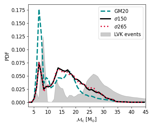
Figure 2: Predicted detectable distribution of chirp mass, for each kick model: GM20 (solid dark-cyan line), $\sigma{}150$ (dotted black line) and $\sigma 265$ (dashed red line). For detectable distribution we mean the distribution of simulated BBHs with sufficiently high signal-to-noise ratio (Section 3). The shaded gray area is the distribution we obtain by stacking the posterior samples of the 59 confident detections from GWTC-3 (Appendix A).

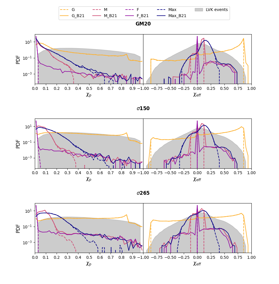
Figure 3: Predicted detectable distribution of $\chi_{\rm p}$ (left) and $\chi_{\rm eff}$ (right) for all of our models. Different colours refer to the spin model: G, M, F and Max. Solid (dashed) lines include (do not include) the tidal spin-up model by B21. From top to bottom: GM20, $\sigma{}150$, and $\sigma{}265$. The shaded gray areas are the distributions we obtain by stacking the posterior samples of the 59 confident detections from GWTC-3 (Appendix A).

3 Hierarchical Bayesian inference

Given a set $\mathcal{H}=\{h^{k}\}_{k=1}^{N_{\rm obs}}$ of $N_{\rm obs}$ GW observations, the posterior distribution of a set of hyper-parameters $\lambda$ associated to an astrophysical model can be described as an in-homogeneous Poisson distribution (e.g., Loredo, 2004; Mandel et al., 2019; Thrane & Talbot, 2019; Bouffanais et al., 2019, 2021a, 2021b):

$$p(\lambda,N_{\lambda}|\mathcal{H})=e^{-\mu_{\lambda}}\,\pi(\lambda,N_{\lambda})\prod^{N_{\rm obs}}_{k=1}N_{\lambda}\int\mathcal{L}^{k}(h^{k}|\theta)\,p(\theta|\lambda)\,\mathrm{d}\theta,$$ (14)

where $N_{\rm obs}$ is the number of events observed by the LVK, with an ensemble of parameters $\theta$, $N_{\lambda}$ is the number of predicted mergers by the model (as calculated in eq. 11), $\mu_{\lambda}$ the number of predicted observations given a model and a detector, $\pi(\lambda,\,{}N_{\lambda})$ are the prior distributions on $\lambda$ and $N_{\lambda}$, and $\mathcal{L}^{k}(\{h\}^{k}|\theta)$ is the likelihood of the $k^{\rm th}$ observation.

The predicted number of events $\mu_{\lambda}$ can be written in terms of detection efficiency $\beta(\lambda)$ for a given model:

$$\mu_{\lambda}=N_{\lambda}\,\beta(\lambda),\quad\mathrm{with}\quad\beta(\lambda)=\int_{\theta}p(\theta|\lambda)\,{}p_{\rm det}(\theta)\,{}\mathrm{d}\theta,$$ (15)

where $p_{\rm det}(\theta{})$ is the detection probability for a set of parameters $\theta$. This probability can be inferred by computing the optimal signal to noise ratio (SNR) of the sources and comparing it to a detection threshold. In our case we chose as reference a threshold $\rho_{\rm thr}=8$ in the LIGO Livingston detector, for which we approximated the sensitivity using the measurements for the three runs separately (Abadie et al., 2010; Abbott et al., 2016b; Wysocki et al., 2018). The values for the event’s log-likelihood were derived from the posterior and prior samples released by the LVK. Hence, the integral in eq. 14 is approximated with a Monte Carlo approach as

$$\mathcal{I}^{k}=\int\mathcal{L}^{k}(h^{k}|\theta)\,{}p(\theta|\lambda)\,{}\mathrm{d}\theta\approx\frac{1}{N^{k}_{s}}\sum^{N^{k}_{s}}_{i=1}\frac{p(\theta_{i}^{k}|\lambda)}{\pi^{k}(\theta^{k}_{i})},$$ (16)

where $\theta^{k}_{i}$ is the $i^{\rm th}$ posterior sample of the $k^{\rm th}$ detection and $N_{s}^{k}$ is the total number of posterior samples for the $k^{\rm th}$ detection. To compute the prior term in the denominator, we also used Gaussian kernel density estimation.

Finally, we can also choose to neglect the information coming from the number of sources predicted by the model when estimating the posterior distribution. By doing so, we can have some insights on the impact of the rate on the analysis. In practice, this can be done by marginalising eq. 14 over $N_{\lambda}$ using a prior $\pi(N_{\lambda})\sim 1/N_{\lambda}$ (Fishbach et al., 2018), which yields to the following expression for a model log-likelihood

$$\mathcal{L}=p(\lambda|\{h^{k}\})\sim\pi(\lambda)\,{}\prod_{k=1}^{N_{\rm obs}}\left[\frac{\mathcal{I}^{k}}{\beta(\lambda)}\right].$$ (17)

We adopted the formalism described in eqs. 14–17 to perform a hierarchical Bayesian inference to compare the astrophysical models presented Sec. 2 with the third gravitational-wave transient catalogue (GWTC-3), the most updated catalogue of gravitational-wave events from the LVK (Abbott et al., 2021b, c). GWTC-3 contains 90 event candidates with probability of astrophysical origin $p_{\rm astro}>0.5$. From GWTC-3, we extract 59 confident detections of BBHs with a false alarm rate ${\rm FAR}<0.25$ yr^-1. In this sub-sample, we do not include binary neutron stars and neutron star – BH systems, and we also exclude the other BBH candidates with an higher FAR. Our chosen FAR threshold ensures a sufficiently pure sample for our analysis (Abbott et al., 2021c). A list of the events used in this study is available in Appendix A. For the observable parameters $\theta$, we use the choice described in Section 2.7, namely $\theta=\{\mathcal{M}_{\rm c},\,{}q,\,{}z,\,{}\chi_{\rm eff},\,{}\chi_{\rm p}\}$.

4 Results

4.1 Chirp mass

The chirp mass distribution (Fig. 2) does not depend on the spin model, by construction. Therefore, we only show different natal kicks. Models $\sigma{}150$ and $\sigma{}265$ show a similar distribution of chirp masses with two peaks of similar importance, one at $\mathcal{M}_{\rm c}\approx{8}$ M_⊙ and the other (broader) peak at $\mathcal{M}_{\rm c}\approx{15}$ M_⊙. In contrast, model GM20 has a much stronger preference for low-mass BHs, with a dominant peak at $\mathcal{M}_{\rm c}\approx{8}$ M_⊙. The reason for this difference is that all BHs in tight binary systems receive slow natal kicks in model GM20 (Fig. 1). This happens because stars in tight binary systems lose their envelope during mass transfer episodes; hence, the mass of supernova ejecta ($m_{\rm ej}$) is small, triggering low kicks in model GM20.

Figure 2 also compares the detectable distribution of our models with the stacked posterior samples from the confident BBH detections in GWTC-3. This figure highlights two main differences between the population synthesis models and the posterior samples: the peak at $\mathcal{M}_{\rm c}\approx{15}$ M_⊙ is stronger in the models than it is in the data, while the data present a more significant excess at $\mathcal{M}_{\rm c}\approx{25-30}$ M_⊙ than the models. Finally, the peak at $\mathcal{M}_{\rm c}\approx{9}$ M_⊙ in the data approximately matches the peak at $\mathcal{M}_{\rm c}\approx{8}$ M_⊙ in the models. The main features of our population synthesis models (in particular, the peaks at $\mathcal{M}_{\rm c}\approx{8-10}$ M_⊙ and $\mathcal{M}_{\rm c}\approx{15-20}$ M_⊙) are also common to other population-synthesis models (e.g., Belczynski et al., 2020; van Son et al., 2022) and mostly spring from the core-collapse SN prescriptions by Fryer et al. (2012). Alternative core-collapse SN models (e.g., Mapelli et al., 2020; Mandel et al., 2021; Patton et al., 2022; Olejak et al., 2022) produce different features and deserve further investigation (Iorio et al., in prep.).

4.2 Spin parameters

Figure 3 shows the detectable distribution of spin parameters $\chi_{\rm p}$ and $\chi_{\rm eff}$ for all of our models. By construction, large spins are much more common in models G and G_B21, while models F and F_B21 have a strong predominance of vanishingly small spins. Models M, M_B21, Max and Max_B21 are intermediate between the other two extreme models.

Including or not the correction by B21 has negligible impact on the distribution of $\chi_{\rm p}$ and $\chi_{\rm eff}$ for models G, because of the predominance of large spin magnitudes. In contrast, introducing the spin-up correction by B21 has a key impact on models F, because it is the only way to account for mild to large spins in these models. The correction by B21 is important also for models M and Max, being responsible for the large-spin wings.

Finally, our model with slow kicks (GM20) results in a distribution of $\chi_{\rm p}$ that is more peaked at zero (for models G, M and Max) with respect to the other two kick models ($\sigma{}150$ and $\sigma{}265$). In fact, the supernova kicks in model GM20 are not large enough to appreciably misalign BH spins (see Fig. 1).

A similar effect is visible in the distribution of $\chi_{\rm eff}$: model $\sigma{}265$ produces a distribution of $\chi_{\rm eff}$ that is less asymmetric about the zero with respect to models $\sigma{}150$ and especially GM20.

4.3 Model Selection

Figure 4 and Table 4 report the values of the log-likelihood $\log\mathcal{L}$ defined in Eq. 17. We can quantify the difference between two models A and B by computing the average absolute difference in percentage

$$\Delta{\rm log}\mathcal{L}({\rm A,\,B})=\left<\frac{2\left|{\rm log}\mathcal{L}_{i}^{\rm A}-{\rm log}\mathcal{L}_{i}^{\rm B}\right|}{{\rm log}\mathcal{L}_{i}^{\rm A}+{\rm log}\mathcal{L}_{i}^{\rm B}}\right>_{var},$$ (18)

on the non-A,B variation $var$ ($var$ would be kick(spin) if A and B are spin(kick) models). For example to compare the two models G and G_B21, A and B become G_B21 and G and $var=\{{\rm GM}20,\,\sigma 150,\,\sigma 265\}$.

The tidal spin-up mechanism (B21) affects the spin of a small part of the population of each model (Fig. 3). However, it improves the likelihood of the F and M models significantly (e.g., $\Delta{\rm log}\mathcal{L}({\rm M\_B21},\,{}{\rm M})=89\%$, Table 4). This improvement of the log-likelihood can be explained by the presence of higher values of $\chi_{\rm p}$ and $\chi_{\rm eff}$ in the distribution of populations M_B21 and F_B21 compared to M and F (Fig. 3).

The F model yields $\mathcal{L}({\rm F})=-\infty{}$ if we do not include the tidal spin-up correction, regardless of the kick model. This indicates that the LVK data do not support vanishingly small BH spins for the entire BBH population. However, it is sufficient to inject a tiny sub-population of spinning BHs, by switching on the B21 correction, and the F model becomes one of the best considered models. In fact, the F_B21 models only includes 0.4% of BHs with $\chi>0.01$ and achieves $\log{\mathcal{L}}>200$ (for spin models $\sigma{150}$ and $\sigma{265}$).

The G and G_B21 spin models exhibit lower log-likelihood values than the others for all kicks models: ${\rm log}\mathcal{L}\leqslant 150$ for $\sigma{150}$ and $\sigma 265$, and ${\rm log}\mathcal{L}<0$ for GM20. This happens because the distribution of $\chi_{\rm eff}$ has non-negligible support for extreme values $\chi_{\rm eff}<-0.5$ and $\chi_{\rm eff}>0.5$ (Fig. 3).

The kick models $\sigma{150}$ and $\sigma 265$ show similar results ($\Delta{\rm log}\mathcal{L}({\rm\sigma{150},{}\sigma 265})<3\%)$ for every spin assumptions. Also, for all spin assumptions, the GM20 kick model scores a significantly lower likelihood than the other models $\sigma{150}$ and $\sigma 265$ with $\Delta{\rm log}\mathcal{L}({\rm\sigma 150,{}{\rm GM20}})\,\sim\,\Delta{\rm log}\mathcal{L}({\rm\sigma 265,{}GM20})\,\sim\,$150%. This result can be explained by the high peak of model GM20 at low chirp masses ($\mathcal{M}_{\rm c}\sim 8{\rm M}_{\odot}$, see Sec.4.1 and Fig.2) and by the low value of $\chi{}_{\rm p}$ compared to the other kick models (Fig. 3).

Models Max and Max_B21 are possibly the best match to the data, but this is not surprising, because they were built as a toy model to visually match the data. Among the astrophysically-motivated models (i.e., after excluding the Max model), M, M_B21 and F_B21 (with kick models $\sigma{150}$ and $\sigma{}265$) are the most favoured by the data. This might be interpreted as a support for the Tayler-Spruit instability mechanism (adopted in models M) and for the tidal spin-up model by B21.

4.4 Importance of $\chi{\rm{}_{p}}$

The $\chi{\rm{}_{p}}$ parameter encodes information on the spin component in the orbital plane. Its impact on gravitational-wave signals is much lower than that of $\chi_{\rm eff}$, and therefore its measurement is less precise. To understand the impact of $\chi_{\rm p}$ on our results, we re-ran the analysis without this parameter. The results are shown in Table 5 and in Fig. 4 with empty markers. Fig. 4 shows that, if we do not include $\chi_{\rm p}$, the models M and M_B21 have almost the same log-likelihood, and even the F model yields a positive log-likelihood. Furthermore, the analysis without $\chi_{\rm p}$ results in significantly larger values of $\mathcal{L}$ for the kick model GM20. Our results demonstrate that the measured $\chi_{\rm p}$ of GWTC-3 BBHs carries substantial information, despite the large uncertainties.

Table 4: Log-likelihood $\mathcal{L}$ (Eq. 17) estimated with five merger parameters $\theta=\left\{\mathcal{M}_{\rm c}\,,z\,,\chi_{\rm eff}\,,q\,,\chi_{\rm p}\right\}$.

Model Name	GM20	$\sigma$150	$\sigma$265
G	-1	149	145
G_B21	-12	150	141
M	0	162	171
M_B21	36	232	232
F	-$\infty$	-$\infty$	-$\infty$
F_B21	88	250	242
Max	92	255	254
Max_B21	106	257	250

Table 5: Log-likelihood $\mathcal{L}$ (Eq. 17) estimated with four merger parameters $\theta=\left\{\mathcal{M}_{\rm c}\,,z\,,\chi_{\rm eff}\,,q\right\}$. Here, we ignore $\chi_{\rm p}$.

Model Name	GM20	$\sigma$150	$\sigma$265
G	35	146	147
G_B21	47	149	154
M	141	192	190
M_B21	130	199	180
F	85	146	138
F_B21	185	207	180
Max	161	208	155
Max_B21	160	206	200

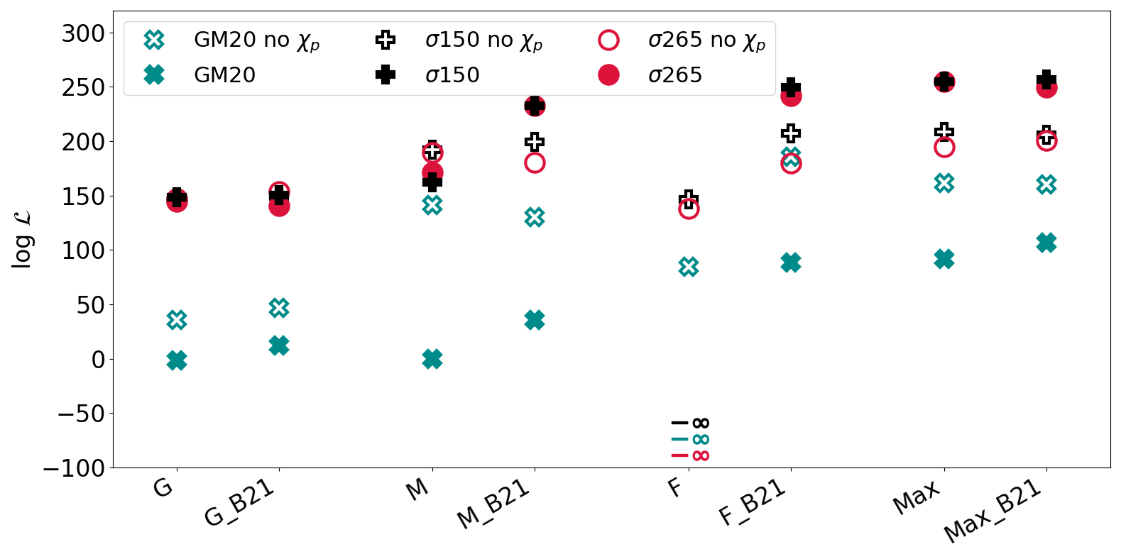
Figure 4: Values of the log-likelihood $\mathcal{L}$ defined in Eq. 17 for the four different models Geneva (G), MESA (M), Fuller (F), and Maxwellian (Max), with/without the tidal spin-up mechanism (B21). Blue crosses: GM20; dark pluses: $\sigma{}150$; red circles: $\sigma{}265$.

5 Discussion

The spin magnitude of BHs is largely uncertain, mostly because we do not fully understand angular momentum transport in massive stars. Here, we have taken a number of spin models bracketing the main uncertainties, we have implemented them into our population-synthesis code mobse, and compared them against GWTC-3 data within a hierarchical Bayesian framework.

The data do not support models in which the entire BH population has vanishingly small spins (model F). This result is mainly driven by the $\chi_{\rm p}$ parameter. This is in agreement with, e.g., the complementary analysis presented in Callister et al. (2022). They employed a variety of complementary methods to measure the distribution of spin magnitudes and orientations of BBH mergers, and concluded that the existence of a sub-population of BHs with vanishing spins is not required by current data. Callister et al. (2022) find that the fraction of non-spinning BHs can comprise up to $\sim{60-70}$% of the total population. In our F_B21 models, we have $\sim{99.6}$% of BHs with $\chi<0.01$.

Recently, Biscoveanu et al. (2021); Roulet et al. (2021); Galaudage et al. (2021) and Tong et al. (2022) claimed the existence of a sub-population of zero-spin BHs. From our analysis, we cannot exclude the existence of such sub-population, as the F model with B21 correction (F_B21) still represents a good match of the data. Similarly to Belczynski et al. (2020) and Gerosa et al. (2018), we find that models with large spins (G, G_B21) are less favoured by the data, but they are still acceptable if we allow for large kicks.

Overall, we find a preference for large natal kicks. This result goes into the same direction as the work by Callister et al. (2021). Actually, this preference for large natal kicks is degenerate with the adopted formation channel. Had we included the dynamical formation channel in dense star clusters, we would have added a sub-population of isotropically oriented spins (see, e.g., Figure 8 of Mapelli et al. 2022). In a forthcoming study, we will extend our analysis to a multi-channel analysis. While it is unlikely that BBH mergers only originate from one single channel, adding more formation channels to a hierarchical Bayesian analysis dramatically increases the number of parameters, making it more difficult to reject some portions of the parameter space.

6 Summary

The origin of BH spins is still controversial, and angular momentum transport inside massive stars is one of the main sources of uncertainty. Here, we apply hierarchical Bayesian inference to derive constraints on spin models from the 59 most confident BBH merger events in GWTC-3. We consider five parameters: chirp mass, mass ratio, redshift, effective spin, and precessing spin.

For model selection, we use a set of binary population synthesis simulations spanning different assumptions for black hole spins and natal kicks. In particular, our spin models account for relatively inefficient (G), efficient (Max and M), and very efficient angular-momentum transport (F). A higher efficiency of angular momentum transport is associated with lower BH spins. In particular, model F predicts vanishingly small spins for the entire BH population. For each of our models, we also include the possibility that some BHs are tidally spun-up (B21). We considered three different natal kick models: according to models $\sigma{}265$ and $\sigma{}150$, we randomly draw the kicks from a Maxwellian curve with $\sigma{}=265$ and 150 km s^-1, respectively; in the third model (G20), we also derive the kicks from a Maxwellian curve with $\sigma{}=265$ km s^-1, but the kick magnitude is then modulated by the ratio between the mass of the ejecta and the mass of the BH.

We summarize our main results as follows.

• The data from GWTC-3 do not support models in which the entire BH population has vanishingly small spins (model F).

• In contrast, models in which most spins are vanishingly small, but that also include a sub-population of tidally spun-up BHs (model F_B21) are a good match to the data.

• The models in which angular momentum transport is relatively inefficient (G and G_21) yield log-likelihood values that are much lower than models with efficient angular momentum transport (M, M_B21, Max, and Max_B21).

• Models with large BH kicks ($\sigma{}150$ and $\sigma{}265$ ) are favoured by our analysis with respect to low-kick models (G20).

• Our results show that the precessing spin parameter $\chi_{\rm p}$ plays a crucial impact to constrain the spin distribution of BBH mergers.

Data Availability

The data underlying this article will be shared on reasonable request to the corresponding author. The latest public version of mobse can be downloaded from this repository. Cosmo$\mathcal{R}$ate can be downlowaded from this link.

Appendix A Sample of gravitational-wave events

Table 6 lists all the gravitational-wave event candidates we used in our study. From GWTC-3, we selected all the event candidates with $p_{\rm astro}>0.9$ and FAR$<0.25$ yr^-1, excluding the following three systems:

• the binary neutron star GW170807;

• the (possible) neutron star–BH binary system GW190814;

• the BBH GW190521 ($m_{1}=98.4^{+33.6}_{-21.7}\mathrm{M}_{\odot}$, $m_{2}=57.2^{+27.1}_{-30.1}\mathrm{M}_{\odot}$ Abbott et al. 2021b), which can form only via dynamical interactions in our models (e.g., Di Carlo et al., 2019; Dall’Amico et al., 2021; Mapelli et al., 2021).

Table 6: Catalogue of BBH events adopted in this study. the ucertainties shown stand for the 90% credible intervals.

Name	$\mathbf{\mathcal{M}_{\rm c}}\mathbf{[M}\mathbf{{}_{\odot}}\mathbf{]}$	$\mathbf{q}$	$\mathbf{\chi_{\rm eff}}$	$\mathbf{\chi_{\rm p}}$	$\mathbf{z}$
GW150914	28.6${}_{-1.5}^{+1.7}$	0.86${}_{-0.2}^{+0.12}$	-0.01${}_{-0.13}^{+0.12}$	0.34${}_{-0.25}^{+0.45}$	0.09${}_{-0.03}^{+0.03}$
GW151012	15.2${}_{-1.2}^{+2.1}$	0.59${}_{-0.35}^{+0.36}$	0.05${}_{-0.2}^{+0.31}$	0.33${}_{-0.25}^{+0.45}$	0.21${}_{-0.09}^{+0.09}$
GW151226	8.9${}_{-0.3}^{+0.3}$	0.56${}_{-0.33}^{+0.38}$	0.18${}_{-0.12}^{+0.2}$	0.49${}_{-0.32}^{+0.39}$	0.09${}_{-0.04}^{+0.04}$
GW170104	21.4${}_{-1.8}^{+2.2}$	0.65${}_{-0.23}^{+0.3}$	-0.04${}_{-0.21}^{+0.17}$	0.36${}_{-0.27}^{+0.42}$	0.2${}_{-0.08}^{+0.08}$
GW170608	7.9${}_{-0.2}^{+0.2}$	0.69${}_{-0.36}^{+0.28}$	0.03${}_{-0.07}^{+0.19}$	0.36${}_{-0.27}^{+0.45}$	0.07${}_{-0.02}^{+0.02}$
GW170729	35.4${}_{-4.8}^{+6.5}$	0.68${}_{-0.28}^{+0.28}$	0.37${}_{-0.25}^{+0.21}$	0.44${}_{-0.28}^{+0.35}$	0.49${}_{-0.21}^{+0.19}$
GW170809	24.9${}_{-1.7}^{+2.1}$	0.68${}_{-0.24}^{+0.28}$	0.08${}_{-0.17}^{+0.17}$	0.35${}_{-0.26}^{+0.43}$	0.2${}_{-0.07}^{+0.05}$
GW170814	24.1${}_{-1.1}^{+1.4}$	0.83${}_{-0.23}^{+0.15}$	0.07${}_{-0.12}^{+0.12}$	0.48${}_{-0.36}^{+0.41}$	0.12${}_{-0.04}^{+0.03}$
GW170818	26.5${}_{-1.7}^{+2.1}$	0.76${}_{-0.25}^{+0.21}$	-0.09${}_{-0.21}^{+0.18}$	0.49${}_{-0.34}^{+0.37}$	0.21${}_{-0.07}^{+0.07}$
GW170823	29.2${}_{-3.6}^{+4.6}$	0.74${}_{-0.3}^{+0.23}$	0.09${}_{-0.26}^{+0.22}$	0.42${}_{-0.31}^{+0.41}$	0.35${}_{-0.15}^{+0.15}$
GW190408_181802	18.3${}_{-1.2}^{+1.9}$	0.75${}_{-0.24}^{+0.21}$	-0.03${}_{-0.19}^{+0.14}$	0.39${}_{-0.31}^{+0.37}$	0.29${}_{-0.1}^{+0.06}$
GW190412	13.3${}_{-0.3}^{+0.4}$	0.28${}_{-0.06}^{+0.12}$	0.25${}_{-0.11}^{+0.08}$	0.3${}_{-0.16}^{+0.19}$	0.15${}_{-0.03}^{+0.03}$
GW190413_052954	24.6${}_{-4.1}^{+5.5}$	0.69${}_{-0.29}^{+0.27}$	-0.01${}_{-0.34}^{+0.29}$	0.41${}_{-0.31}^{+0.43}$	0.59${}_{-0.24}^{+0.29}$
GW190413_134308	33.0${}_{-5.4}^{+8.2}$	0.69${}_{-0.31}^{+0.28}$	-0.03${}_{-0.29}^{+0.25}$	0.56${}_{-0.41}^{+0.37}$	0.71${}_{-0.3}^{+0.31}$
GW190421_213856	31.2${}_{-4.2}^{+5.9}$	0.79${}_{-0.3}^{+0.19}$	-0.06${}_{-0.27}^{+0.22}$	0.48${}_{-0.36}^{+0.4}$	0.49${}_{-0.21}^{+0.19}$
GW190503_185404	30.2${}_{-4.2}^{+4.2}$	0.65${}_{-0.23}^{+0.29}$	-0.03${}_{-0.26}^{+0.2}$	0.38${}_{-0.29}^{+0.42}$	0.27${}_{-0.11}^{+0.11}$
GW190512_180714	14.6${}_{-1.0}^{+1.3}$	0.54${}_{-0.18}^{+0.37}$	0.03${}_{-0.13}^{+0.12}$	0.22${}_{-0.17}^{+0.37}$	0.27${}_{-0.1}^{+0.09}$
GW190513_205428	21.6${}_{-1.9}^{+3.8}$	0.5${}_{-0.18}^{+0.42}$	0.11${}_{-0.17}^{+0.28}$	0.31${}_{-0.23}^{+0.39}$	0.37${}_{-0.13}^{+0.13}$
GW190517_055101	26.6${}_{-4.0}^{+4.0}$	0.68${}_{-0.29}^{+0.27}$	0.52${}_{-0.19}^{+0.19}$	0.49${}_{-0.29}^{+0.3}$	0.34${}_{-0.14}^{+0.24}$
GW190519_153544	44.5${}_{-7.1}^{+6.4}$	0.61${}_{-0.19}^{+0.28}$	0.31${}_{-0.22}^{+0.2}$	0.44${}_{-0.29}^{+0.35}$	0.44${}_{-0.14}^{+0.25}$
GW190521_074359	32.1${}_{-2.5}^{+3.2}$	0.78${}_{-0.21}^{+0.19}$	0.09${}_{-0.13}^{+0.1}$	0.4${}_{-0.29}^{+0.32}$	0.24${}_{-0.1}^{+0.07}$
GW190602_175927	49.1${}_{-8.5}^{+9.1}$	0.71${}_{-0.33}^{+0.25}$	0.07${}_{-0.24}^{+0.25}$	0.42${}_{-0.31}^{+0.41}$	0.47${}_{-0.17}^{+0.25}$
GW190620_030421	38.3${}_{-6.5}^{+8.3}$	0.62${}_{-0.27}^{+0.32}$	0.33${}_{-0.25}^{+0.22}$	0.43${}_{-0.28}^{+0.36}$	0.49${}_{-0.2}^{+0.23}$
GW190630_185205	24.9${}_{-2.1}^{+2.1}$	0.68${}_{-0.22}^{+0.27}$	0.1${}_{-0.13}^{+0.12}$	0.32${}_{-0.23}^{+0.31}$	0.18${}_{-0.07}^{+0.1}$
GW190701_203306	40.3${}_{-4.9}^{+5.4}$	0.76${}_{-0.31}^{+0.21}$	-0.07${}_{-0.29}^{+0.23}$	0.42${}_{-0.31}^{+0.42}$	0.37${}_{-0.12}^{+0.11}$
GW190706_222641	42.7${}_{-7.0}^{+10.0}$	0.58${}_{-0.25}^{+0.34}$	0.28${}_{-0.29}^{+0.26}$	0.38${}_{-0.28}^{+0.39}$	0.71${}_{-0.27}^{+0.32}$
GW190707_093326	8.5${}_{-0.5}^{+0.6}$	0.73${}_{-0.27}^{+0.24}$	-0.05${}_{-0.08}^{+0.1}$	0.29${}_{-0.23}^{+0.39}$	0.16${}_{-0.07}^{+0.07}$
GW190708_232457	13.2${}_{-0.6}^{+0.9}$	0.76${}_{-0.28}^{+0.21}$	0.02${}_{-0.08}^{+0.1}$	0.29${}_{-0.23}^{+0.43}$	0.18${}_{-0.07}^{+0.06}$
GW190720_000836	8.9${}_{-0.8}^{+0.5}$	0.58${}_{-0.3}^{+0.36}$	0.18${}_{-0.12}^{+0.14}$	0.33${}_{-0.22}^{+0.43}$	0.16${}_{-0.06}^{+0.12}$
GW190727_060333	28.6${}_{-3.7}^{+5.3}$	0.8${}_{-0.32}^{+0.18}$	0.11${}_{-0.25}^{+0.26}$	0.47${}_{-0.36}^{+0.41}$	0.55${}_{-0.22}^{+0.21}$
GW190728_064510	8.6${}_{-0.3}^{+0.5}$	0.66${}_{-0.37}^{+0.3}$	0.12${}_{-0.07}^{+0.2}$	0.29${}_{-0.2}^{+0.37}$	0.18${}_{-0.07}^{+0.05}$
GW190803_022701	27.3${}_{-4.1}^{+5.7}$	0.75${}_{-0.31}^{+0.22}$	-0.03${}_{-0.27}^{+0.24}$	0.44${}_{-0.33}^{+0.42}$	0.55${}_{-0.24}^{+0.26}$
GW190828_063405	25.0${}_{-2.1}^{+3.4}$	0.82${}_{-0.22}^{+0.15}$	0.19${}_{-0.16}^{+0.15}$	0.43${}_{-0.3}^{+0.36}$	0.38${}_{-0.15}^{+0.1}$
GW190828_065509	13.3${}_{-1.0}^{+1.2}$	0.43${}_{-0.16}^{+0.38}$	0.08${}_{-0.16}^{+0.16}$	0.3${}_{-0.23}^{+0.38}$	0.3${}_{-0.1}^{+0.1}$
GW190910_112807	34.3${}_{-4.1}^{+4.1}$	0.82${}_{-0.23}^{+0.15}$	0.02${}_{-0.18}^{+0.18}$	0.4${}_{-0.32}^{+0.39}$	0.28${}_{-0.1}^{+0.16}$
GW190915_235702	25.3${}_{-2.7}^{+3.2}$	0.69${}_{-0.27}^{+0.27}$	0.02${}_{-0.25}^{+0.2}$	0.55${}_{-0.39}^{+0.36}$	0.3${}_{-0.1}^{+0.11}$
GW190924_021846	5.8${}_{-0.2}^{+0.2}$	0.57${}_{-0.37}^{+0.36}$	0.03${}_{-0.09}^{+0.3}$	0.24${}_{-0.18}^{+0.4}$	0.12${}_{-0.04}^{+0.04}$
GW190925_232845	15.8${}_{-1.0}^{+1.1}$	0.73${}_{-0.34}^{+0.24}$	0.11${}_{-0.14}^{+0.17}$	0.39${}_{-0.29}^{+0.43}$	0.19${}_{-0.07}^{+0.07}$
GW190930_133541	8.5${}_{-0.5}^{+0.5}$	0.64${}_{-0.45}^{+0.3}$	0.14${}_{-0.15}^{+0.31}$	0.34${}_{-0.24}^{+0.4}$	0.15${}_{-0.06}^{+0.06}$
GW191105_143521	7.8${}_{-0.4}^{+0.6}$	0.72${}_{-0.31}^{+0.24}$	-0.02${}_{-0.09}^{+0.13}$	0.3${}_{-0.24}^{+0.45}$	0.23${}_{-0.09}^{+0.07}$
GW191109_010717	47.5${}_{-7.5}^{+9.6}$	0.73${}_{-0.24}^{+0.21}$	-0.29${}_{-0.31}^{+0.42}$	0.63${}_{-0.37}^{+0.29}$	0.25${}_{-0.12}^{+0.18}$
GW191129_134029	7.3${}_{-0.3}^{+0.4}$	0.63${}_{-0.29}^{+0.31}$	0.06${}_{-0.08}^{+0.16}$	0.26${}_{-0.19}^{+0.36}$	0.16${}_{-0.06}^{+0.05}$
GW191204_171526	8.6${}_{-0.3}^{+0.4}$	0.69${}_{-0.26}^{+0.25}$	0.16${}_{-0.05}^{+0.08}$	0.39${}_{-0.26}^{+0.35}$	0.13${}_{-0.05}^{+0.04}$
GW191215_223052	18.4${}_{-1.7}^{+2.2}$	0.73${}_{-0.27}^{+0.24}$	-0.04${}_{-0.21}^{+0.17}$	0.5${}_{-0.38}^{+0.37}$	0.35${}_{-0.14}^{+0.13}$
GW191216_213338	8.3${}_{-0.2}^{+0.2}$	0.64${}_{-0.29}^{+0.31}$	0.11${}_{-0.06}^{+0.13}$	0.23${}_{-0.16}^{+0.35}$	0.07${}_{-0.03}^{+0.02}$
GW191222_033537	33.8${}_{-5.0}^{+7.1}$	0.79${}_{-0.32}^{+0.18}$	-0.04${}_{-0.25}^{+0.2}$	0.41${}_{-0.32}^{+0.41}$	0.51${}_{-0.26}^{+0.23}$
GW191230_180458	36.5${}_{-5.6}^{+8.2}$	0.77${}_{-0.34}^{+0.2}$	-0.05${}_{-0.31}^{+0.26}$	0.52${}_{-0.39}^{+0.38}$	0.69${}_{-0.27}^{+0.26}$
GW200112_155838	27.4${}_{-2.1}^{+2.6}$	0.81${}_{-0.26}^{+0.17}$	0.06${}_{-0.15}^{+0.15}$	0.39${}_{-0.3}^{+0.39}$	0.24${}_{-0.08}^{+0.07}$
GW200128_022011	32.0${}_{-5.5}^{+7.5}$	0.8${}_{-0.3}^{+0.18}$	0.12${}_{-0.25}^{+0.24}$	0.57${}_{-0.4}^{+0.34}$	0.56${}_{-0.28}^{+0.28}$
GW200129_065458	27.2${}_{-2.3}^{+2.1}$	0.85${}_{-0.41}^{+0.12}$	0.11${}_{-0.16}^{+0.11}$	0.52${}_{-0.37}^{+0.42}$	0.18${}_{-0.07}^{+0.05}$
GW200202_154313	7.5${}_{-0.2}^{+0.2}$	0.72${}_{-0.31}^{+0.24}$	0.04${}_{-0.06}^{+0.13}$	0.28${}_{-0.22}^{+0.4}$	0.09${}_{-0.03}^{+0.03}$
GW200208_130117	27.7${}_{-3.1}^{+3.6}$	0.73${}_{-0.29}^{+0.23}$	-0.07${}_{-0.27}^{+0.22}$	0.38${}_{-0.29}^{+0.41}$	0.4${}_{-0.14}^{+0.15}$
GW200209_085452	26.7${}_{-4.2}^{+6.0}$	0.78${}_{-0.31}^{+0.19}$	-0.12${}_{-0.3}^{+0.24}$	0.51${}_{-0.37}^{+0.39}$	0.57${}_{-0.26}^{+0.25}$
GW200219_094415	27.6${}_{-3.8}^{+5.6}$	0.77${}_{-0.32}^{+0.21}$	-0.08${}_{-0.29}^{+0.23}$	0.48${}_{-0.35}^{+0.4}$	0.57${}_{-0.22}^{+0.22}$
GW200224_222234	31.1${}_{-2.6}^{+3.2}$	0.82${}_{-0.26}^{+0.16}$	0.1${}_{-0.15}^{+0.15}$	0.49${}_{-0.36}^{+0.37}$	0.32${}_{-0.11}^{+0.08}$
GW200225_060421	14.2${}_{-1.4}^{+1.5}$	0.73${}_{-0.28}^{+0.23}$	-0.12${}_{-0.28}^{+0.17}$	0.53${}_{-0.38}^{+0.34}$	0.22${}_{-0.1}^{+0.09}$
GW200302_015811	23.4${}_{-3.0}^{+4.7}$	0.53${}_{-0.2}^{+0.36}$	0.01${}_{-0.26}^{+0.25}$	0.37${}_{-0.28}^{+0.45}$	0.28${}_{-0.12}^{+0.16}$
GW200311_115853	26.6${}_{-2.0}^{+2.4}$	0.82${}_{-0.27}^{+0.16}$	-0.02${}_{-0.2}^{+0.16}$	0.45${}_{-0.35}^{+0.4}$	0.23${}_{-0.07}^{+0.05}$
GW200316_215756	8.8${}_{-0.6}^{+0.6}$	0.6${}_{-0.38}^{+0.34}$	0.13${}_{-0.1}^{+0.27}$	0.29${}_{-0.2}^{+0.38}$	0.22${}_{-0.08}^{+0.08}$

References

- Aasi et al. (2015) Aasi J., et al., 2015, Classical and Quantum Gravity, 32, 074001
- Abadie et al. (2010) Abadie J., et al., 2010, Classical and Quantum Gravity, 27, 173001
- Abbott et al. (2016a) Abbott B. P., et al., 2016a, Phys. Rev. Lett., 116, 241103
- Abbott et al. (2016b) Abbott B. P., et al., 2016b, ApJ, 833, L1
- Abbott et al. (2019) Abbott B. P., et al., 2019, Physical Review X, 9, 031040
- Abbott et al. (2020) Abbott R., et al., 2020, Phys. Rev. D, 102, 043015
- Abbott et al. (2021a) Abbott R., et al., 2021a, arXiv e-prints, p. arXiv:2108.01045
- Abbott et al. (2021b) Abbott R., et al., 2021b, arXiv e-prints, p. arXiv:2111.03606
- Abbott et al. (2021c) Abbott R., et al., 2021c, arXiv e-prints, p. arXiv:2111.03634
- Abbott et al. (2021d) Abbott R., et al., 2021d, Physical Review X, 11, 021053
- Abbott et al. (2021e) Abbott R., et al., 2021e, SoftwareX, 13, 100658
- Acernese et al. (2015) Acernese F., et al., 2015, Classical and Quantum Gravity, 32, 024001
- Aerts et al. (2019) Aerts C., Mathis S., Rogers T. M., 2019, ARA&A, 57, 35
- Aghanim et al. (2020) Aghanim N., et al., 2020, A&A, 641, A6
- Arca Sedda & Benacquista (2019) Arca Sedda M., Benacquista M., 2019, MNRAS, 482, 2991
- Arca Sedda et al. (2020) Arca Sedda M., Mapelli M., Spera M., Benacquista M., Giacobbo N., 2020, ApJ, 894, 133
- Atri et al. (2019) Atri P., et al., 2019, MNRAS, 489, 3116
- Baibhav et al. (2020) Baibhav V., Gerosa D., Berti E., Wong K. W. K., Helfer T., Mould M., 2020, Phys. Rev. D, 102, 043002
- Barrett et al. (2018) Barrett J. W., Gaebel S. M., Neijssel C. J., Vigna-Gómez A., Stevenson S., Berry C. P. L., Farr W. M., Mandel I., 2018, MNRAS, 477, 4685
- Bavera et al. (2020) Bavera S. S., et al., 2020, A&A, 635, A97
- Bavera et al. (2021) Bavera S. S., Zevin M., Fragos T., 2021, Research Notes of the American Astronomical Society, 5, 127
- Belczynski et al. (2010) Belczynski K., Bulik T., Fryer C. L., Ruiter A., Valsecchi F., Vink J. S., Hurley J. R., 2010, ApJ, 714, 1217
- Belczynski et al. (2020) Belczynski K., et al., 2020, A&A, 636, A104
- Biscoveanu et al. (2021) Biscoveanu S., Isi M., Vitale S., Varma V., 2021, Phys. Rev. Lett., 126, 171103
- Bouffanais et al. (2019) Bouffanais Y., Mapelli M., Gerosa D., Di Carlo U. N., Giacobbo N., Berti E., Baibhav V., 2019, ApJ, 886, 25
- Bouffanais et al. (2021a) Bouffanais Y., Mapelli M., Santoliquido F., Giacobbo N., Iorio G., Costa G., 2021a, MNRAS, 505, 3873
- Bouffanais et al. (2021b) Bouffanais Y., Mapelli M., Santoliquido F., Giacobbo N., Di Carlo U. N., Rastello S., Artale M. C., Iorio G., 2021b, MNRAS, 507, 5224
- Briel et al. (2022) Briel M. M., Stevance H. F., Eldridge J. J., 2022, arXiv e-prints, p. arXiv:2206.13842
- Broekgaarden et al. (2022a) Broekgaarden F. S., et al., 2022a, MNRAS, 516, 5737
- Broekgaarden et al. (2022b) Broekgaarden F. S., Stevenson S., Thrane E., 2022b, ApJ, 938, 45
- Callister et al. (2021) Callister T. A., Farr W. M., Renzo M., 2021, ApJ, 920, 157
- Callister et al. (2022) Callister T. A., Miller S. J., Chatziioannou K., Farr W. M., 2022, arXiv e-prints, p. arXiv:2205.08574
- Cantiello et al. (2014) Cantiello M., Mankovich C., Bildsten L., Christensen-Dalsgaard J., Paxton B., 2014, ApJ, 788, 93
- Chattopadhyay et al. (2022) Chattopadhyay D., Hurley J., Stevenson S., Raidani A., 2022, MNRAS, 513, 4527
- Claeys et al. (2014) Claeys J. S. W., Pols O. R., Izzard R. G., Vink J., Verbunt F. W. M., 2014, A&A, 563, A83
- Costa et al. (2019) Costa G., Girardi L., Bressan A., Marigo P., Rodrigues T. S., Chen Y., Lanza A., Goudfrooij P., 2019, MNRAS, 485, 4641
- Dall’Amico et al. (2021) Dall’Amico M., Mapelli M., Di Carlo U. N., Bouffanais Y., Rastello S., Santoliquido F., Ballone A., Arca Sedda M., 2021, MNRAS, 508, 3045
- Di Carlo et al. (2019) Di Carlo U. N., Giacobbo N., Mapelli M., Pasquato M., Spera M., Wang L., Haardt F., 2019, MNRAS, 487, 2947
- Ekström et al. (2012) Ekström S., et al., 2012, A&A, 537, A146
- Eldridge & Stanway (2016) Eldridge J. J., Stanway E. R., 2016, MNRAS, 462, 3302
- Farr et al. (2011) Farr W. M., Sravan N., Cantrell A., Kreidberg L., Bailyn C. D., Mandel I., Kalogera V., 2011, ApJ, 741, 103
- Farr et al. (2017) Farr W. M., Stevenson S., Miller M. C., Mandel I., Farr B., Vecchio A., 2017, Nature, 548, 426
- Farr et al. (2018) Farr B., Holz D. E., Farr W. M., 2018, ApJ, 854, L9
- Fishbach & Holz (2017) Fishbach M., Holz D. E., 2017, ApJ, 851, L25
- Fishbach & Kalogera (2022) Fishbach M., Kalogera V., 2022, ApJ, 929, L26
- Fishbach et al. (2018) Fishbach M., Holz D. E., Farr W. M., 2018, The Astrophysical Journal, 863, L41
- Fragione & Kocsis (2020) Fragione G., Kocsis B., 2020, Mon. Not. Roy. Astron. Soc., 493, 3920
- Fragione et al. (2022) Fragione G., Kocsis B., Rasio F. A., Silk J., 2022, Astrophys. J., 927, 231
- Fragos & McClintock (2015) Fragos T., McClintock J. E., 2015, ApJ, 800, 17
- Fryer & Kalogera (2001) Fryer C. L., Kalogera V., 2001, ApJ, 554, 548
- Fryer et al. (2012) Fryer C. L., Belczynski K., Wiktorowicz G., Dominik M., Kalogera V., Holz D. E., 2012, ApJ, 749, 91
- Fryer et al. (2022) Fryer C. L., Olejak A., Belczynski K., 2022, ApJ, 931, 94
- Fuller & Ma (2019) Fuller J., Ma L., 2019, ApJ, 881, L1
- Fuller et al. (2019) Fuller J., Piro A. L., Jermyn A. S., 2019, MNRAS, 485, 3661
- Galaudage et al. (2021) Galaudage S., Talbot C., Nagar T., Jain D., Thrane E., Mandel I., 2021, ApJ, 921, L15
- Gehan et al. (2018) Gehan C., Mosser B., Michel E., Samadi R., Kallinger T., 2018, A&A, 616, A24
- Gerosa et al. (2013) Gerosa D., Kesden M., Berti E., O’Shaughnessy R., Sperhake U., 2013, Phys. Rev. D, 87, 104028
- Gerosa et al. (2018) Gerosa D., Berti E., O’Shaughnessy R., Belczynski K., Kesden M., Wysocki D., Gladysz W., 2018, Phys. Rev. D, 98, 084036
- Giacobbo & Mapelli (2018) Giacobbo N., Mapelli M., 2018, MNRAS, 480, 2011
- Giacobbo & Mapelli (2019) Giacobbo N., Mapelli M., 2019, MNRAS, 482, 2234
- Giacobbo & Mapelli (2020) Giacobbo N., Mapelli M., 2020, ApJ, 891, 141
- Giacobbo et al. (2018) Giacobbo N., Mapelli M., Spera M., 2018, MNRAS, 474, 2959
- Hannam et al. (2022) Hannam M., et al., 2022, Nature, 610, 652
- Harris et al. (2020) Harris C. R., et al., 2020, Nature, 585, 357
- Heger et al. (2003) Heger A., Fryer C. L., Woosley S. E., Langer N., Hartmann D. H., 2003, ApJ, 591, 288
- Hobbs et al. (2005) Hobbs G., Lorimer D. R., Lyne A. G., Kramer M., 2005, MNRAS, 360, 974
- Hotokezaka & Piran (2017) Hotokezaka K., Piran T., 2017, ApJ, 842, 111
- Hunter (2007) Hunter J. D., 2007, Computing in Science & Engineering, 9, 90
- Hurley et al. (2000) Hurley J. R., Pols O. R., Tout C. A., 2000, MNRAS, 315, 543
- Hurley et al. (2002) Hurley J. R., Tout C. A., Pols O. R., 2002, MNRAS, 329, 897
- Kalogera (2000) Kalogera V., 2000, ApJ, 541, 319
- Kimball et al. (2020) Kimball C., Talbot C., Berry C. P. L., Carney M., Zevin M., Thrane E., Kalogera V., 2020, ApJ, 900, 177
- Kimball et al. (2021) Kimball C., et al., 2021, Astrophys. J. Lett., 915, L35
- Kroupa (2001) Kroupa P., 2001, MNRAS, 322, 231
- Kushnir et al. (2016) Kushnir D., Zaldarriaga M., Kollmeier J. A., Waldman R., 2016, MNRAS, 462, 844
- Limongi & Chieffi (2018) Limongi M., Chieffi A., 2018, ApJS, 237, 13
- Loredo (2004) Loredo T. J., 2004, in Fischer R., Preuss R., Toussaint U. V., eds, American Institute of Physics Conference Series Vol. 735, Bayesian Inference and Maximum Entropy Methods in Science and Engineering: 24th International Workshop on Bayesian Inference and Maximum Entropy Methods in Science and Engineering. pp 195–206 (arXiv:astro-ph/0409387), doi:10.1063/1.1835214
- Maccarone et al. (2007) Maccarone T. J., Kundu A., Zepf S. E., Rhode K. L., 2007, Nature, 445, 183
- Madau & Fragos (2017) Madau P., Fragos T., 2017, ApJ, 840, 39
- Maeder & Meynet (2000) Maeder A., Meynet G., 2000, ARA&A, 38, 143
- Mandel et al. (2019) Mandel I., Farr W. M., Gair J. R., 2019, MNRAS, 486, 1086
- Mandel et al. (2021) Mandel I., Müller B., Riley J., de Mink S. E., Vigna-Gómez A., Chattopadhyay D., 2021, MNRAS, 500, 1380
- Mapelli et al. (2013) Mapelli M., Zampieri L., Ripamonti E., Bressan A., 2013, MNRAS, 429, 2298
- Mapelli et al. (2017) Mapelli M., Giacobbo N., Ripamonti E., Spera M., 2017, MNRAS, 472, 2422
- Mapelli et al. (2020) Mapelli M., Spera M., Montanari E., Limongi M., Chieffi A., Giacobbo N., Bressan A., Bouffanais Y., 2020, ApJ, 888, 76
- Mapelli et al. (2021) Mapelli M., et al., 2021, MNRAS, 505, 339
- Mapelli et al. (2022) Mapelli M., Bouffanais Y., Santoliquido F., Arca Sedda M., Artale M. C., 2022, MNRAS, 511, 5797
- Marchant et al. (2016) Marchant P., Langer N., Podsiadlowski P., Tauris T. M., Moriya T. J., 2016, A&A, 588, A50
- Miller-Jones et al. (2021) Miller-Jones J. C. A., et al., 2021, Science, 371, 1046
- Miller et al. (2020) Miller S., Callister T. A., Farr W. M., 2020, ApJ, 895, 128
- Mosser et al. (2012) Mosser B., et al., 2012, A&A, 548, A10
- Motta et al. (2014) Motta S. E., Belloni T. M., Stella L., Muñoz-Darias T., Fender R., 2014, MNRAS, 437, 2554
- Olejak & Belczynski (2021) Olejak A., Belczynski K., 2021, ApJ, 921, L2
- Olejak et al. (2022) Olejak A., Fryer C. L., Belczynski K., Baibhav V., 2022, MNRAS, 516, 2252
- Olsen et al. (2022) Olsen S., Venumadhav T., Mushkin J., Roulet J., Zackay B., Zaldarriaga M., 2022, Phys. Rev. D, 106, 043009
- Özel et al. (2010) Özel F., Psaltis D., Narayan R., McClintock J. E., 2010, ApJ, 725, 1918
- Patton et al. (2022) Patton R. A., Sukhbold T., Eldridge J. J., 2022, MNRAS, 511, 903
- Perna et al. (2022) Perna R., Artale M. C., Wang Y.-H., Mapelli M., Lazzati D., Sgalletta C., Santoliquido F., 2022, MNRAS, 512, 2654
- Qin et al. (2018) Qin Y., Fragos T., Meynet G., Andrews J., Sørensen M., Song H. F., 2018, A&A, 616, A28
- Qin et al. (2019) Qin Y., Fragos T., Meynet G., Marchant P., Kalogera V., Andrews J., Sørensen M., Song H. F., 2019, IAU Symposium, 346, 426
- Repetto et al. (2017) Repetto S., Igoshev A. P., Nelemans G., 2017, MNRAS, 467, 298
- Reynolds (2021) Reynolds C. S., 2021, ARA&A, 59, 117
- Rodriguez et al. (2016) Rodriguez C. L., Zevin M., Pankow C., Kalogera V., Rasio F. A., 2016, ApJ, 832, L2
- Roulet & Zaldarriaga (2019) Roulet J., Zaldarriaga M., 2019, MNRAS, 484, 4216
- Roulet et al. (2021) Roulet J., Chia H. S., Olsen S., Dai L., Venumadhav T., Zackay B., Zaldarriaga M., 2021, Phys. Rev. D, 104, 083010
- Sana et al. (2012) Sana H., et al., 2012, Science, 337, 444
- Santoliquido et al. (2020) Santoliquido F., Mapelli M., Bouffanais Y., Giacobbo N., Di Carlo U. N., Rastello S., Artale M. C., Ballone A., 2020, ApJ, 898, 152
- Santoliquido et al. (2021) Santoliquido F., Mapelli M., Giacobbo N., Bouffanais Y., Artale M. C., 2021, MNRAS, 502, 4877
- Shafee et al. (2006) Shafee R., McClintock J. E., Narayan R., Davis S. W., Li L.-X., Remillard R. A., 2006, ApJ, 636, L113
- Spera & Mapelli (2017) Spera M., Mapelli M., 2017, MNRAS, 470, 4739
- Spruit (2002) Spruit H. C., 2002, A&A, 381, 923
- Stegmann & Antonini (2021) Stegmann J., Antonini F., 2021, Phys. Rev. D, 103, 063007
- Stevenson (2022) Stevenson S., 2022, ApJ, 926, L32
- Stevenson & Clarke (2022) Stevenson S., Clarke T. A., 2022, MNRAS,
- Stevenson et al. (2015) Stevenson S., Ohme F., Fairhurst S., 2015, ApJ, 810, 58
- Stevenson et al. (2017) Stevenson S., Berry C. P. L., Mandel I., 2017, MNRAS, 471, 2801
- Talbot & Thrane (2017) Talbot C., Thrane E., 2017, Phys. Rev. D, 96, 023012
- Tauris et al. (2015) Tauris T. M., Langer N., Podsiadlowski P., 2015, MNRAS, 451, 2123
- Tauris et al. (2017) Tauris T. M., et al., 2017, ApJ, 846, 170
- Taylor & Gerosa (2018) Taylor S. R., Gerosa D., 2018, Phys. Rev. D, 98, 083017
- The LIGO Scientific Collaboration et al. (2023) The LIGO Scientific Collaboration et al., 2023, arXiv e-prints, p. arXiv:2302.03676
- Thrane & Talbot (2019) Thrane E., Talbot C., 2019, Publ. Astron. Soc. Australia, 36, e010
- Tiwari et al. (2018) Tiwari V., Fairhurst S., Hannam M., 2018, ApJ, 868, 140
- Tong et al. (2022) Tong H., Galaudage S., Thrane E., 2022, Phys. Rev. D, 106, 103019
- Venumadhav et al. (2020) Venumadhav T., Zackay B., Roulet J., Dai L., Zaldarriaga M., 2020, Phys. Rev. D, 101, 083030
- Vink et al. (2001) Vink J. S., de Koter A., Lamers H. J. G. L. M., 2001, A&A, 369, 574
- Virtanen et al. (2020) Virtanen P., et al., 2020, Nature Methods, 17, 261
- Vitale et al. (2017) Vitale S., Lynch R., Sturani R., Graff P., 2017, Classical and Quantum Gravity, 34, 03LT01
- Wysocki et al. (2018) Wysocki D., Gerosa D., O’Shaughnessy R., Belczynski K., Gladysz W., Berti E., Kesden M., Holz D. E., 2018, Phys. Rev. D, 97, 043014
- Wysocki et al. (2019) Wysocki D., Lange J., O’Shaughnessy R., 2019, Phys. Rev. D, 100, 043012
- Zahn (1992) Zahn J. P., 1992, A&A, 265, 115
- Zaldarriaga et al. (2018) Zaldarriaga M., Kushnir D., Kollmeier J. A., 2018, MNRAS, 473, 4174
- Zevin et al. (2017) Zevin M., Pankow C., Rodriguez C. L., Sampson L., Chase E., Kalogera V., Rasio F. A., 2017, ApJ, 846, 82
- Zevin et al. (2021) Zevin M., et al., 2021, ApJ, 910, 152
- de Mink & Mandel (2016) de Mink S. E., Mandel I., 2016, MNRAS, 460, 3545
- van Son et al. (2022) van Son L. A. C., et al., 2022, Astrophys. J., 940, 184