Velocity waves in the Hubble diagram: signature of local galaxy clusters

Abstract

The Universe expansion rate is modulated around local inhomogeneities due to their gravitational potential. Velocity waves are then observed around galaxy clusters in the Hubble diagram. This paper studies them in a $\sim$738 Mpc wide, with 2048³ particles, cosmological simulation of our cosmic environment (a.k.a. CLONE: Constrained LOcal & Nesting Environment Simulation). For the first time, the simulation shows that velocity waves that arise in the lines-of-sight of the most massive dark matter halos agree with those observed in local galaxy velocity catalogs in the lines-of-sight of Coma and several other local (Abell) clusters. For the best-constrained clusters such as Virgo and Centaurus, i.e. those closest to us, secondary waves caused by galaxy groups, further into the non-linear regime, also stand out. This match is not utterly expected given that before being evolved into a fully non-linear z=0 state, assuming $\Lambda$CDM, CLONE initial conditions are constrained with solely linear theory, power spectrum and highly uncertain and sparse local peculiar velocities. Additionally, Gaussian fits to velocity wave envelopes show that wave properties are tightly tangled with cluster masses. This link is complex though and involves the environment and formation history of the clusters. Using machine learning techniques to grasp more thoroughly the complex wave-mass relation, velocity waves could in the near future be used to provide additional and independent mass estimates from galaxy dynamics within large cluster radii.

1 Introduction

As the largest gravitationally bound structures in the Universe, galaxy clusters bear imprints of the cosmic growth visible through the distribution and motion of galaxies in their surrounding environment (see Kravtsov & Borgani, 2012, for a review and references therein). They constitute therefore powerful complementary probes to supernovae and baryon acoustic oscillations in testing theories explaining cosmic acceleration origin (see Weinberg et al., 2013, for a review). Relations between halo masses and observables (optical galaxy richness, Sunyaev-Zel’dovich effect, X-ray luminosity) must however be calibrated beforehand to study the evolution of the cluster mass function. Our capacity to discriminate among cosmological models is thus tightly linked to the accuracy of cluster mass estimates. However, most of the cluster matter content is not directly visible making their mass estimates a particularly challenging task (see for a review Pratt et al., 2019; Planck Collaboration et al., 2016).

With future imaging surveys to come (Burke, 2006, LSST,; Peacock, 2008, Euclid,; Green et al., 2012, WFIRST,), stacked weak lensing measurements will certainly provide the best cluster mass estimates, i.e. with the 1% accuracy required (Mandelbaum et al., 2006) but limited to small radii around clusters. Independent virial mass estimators (Heisler et al., 1985), hydrostatic estimators for galaxy population (Carlberg et al., 1997) or velocity caustics (boundaries between galaxies bound to and escaping from the cluster potential, Diaferio, 1999) constitute complementary tools once calibrated. Their calibration suffers though from the influence of baryonic physics and galaxy bias on velocity fields and dispersion profiles. Perhaps velocity caustics are less prone to such systematics (Diaferio, 1999) explaining their recent increased popularity. Galaxy clusters can indeed be seen as disrupters of the expansion, thus creating a velocity wave first mentioned by Tonry & Davis (1981) as a triple-value region whose properties (mostly height and width) depend on the cluster mass. Combined with infall models (Mohayaee & Tully, 2005), velocities of galaxies in the infall zones constitute thus good mass proxies for galaxy clusters shown to be in good agreement with virial mass estimates (Tully, 2015). They have been used in different studies to retrieve the total amount of dark matter in groups and clusters as well as to detect groups (e.g. Karachentsev et al., 2013; Karachentsev & Nasonova, 2013). Moreover, Zu et al. (2014) showed that the wave shape is an excellent complementary probe: for instance, f(R) modified gravity models enhance the wave height (infall velocity) and broaden its width (velocity dispersions). This translates into a higher mass when considering a $\Lambda$CDM framework. Subsequently, it would lead to cosmological tensions between $S_{8}$ values measured with the cosmic microwave background and with the galaxy cluster counts. Furthermore, velocity waves probe a cluster mass within radii larger than those reached with weak lensing. Subsequently, combined together, stacked weak lensing and velocity wave mass measurements hold tighter constraints on dark energy than each of them separately. Indeed, velocity waves are signatures of a tug of war between gravity and dark energy. Differences between these two independent mass estimates, one dynamic and one static, permit measuring the gravitational slip between the Newtonian and curvature potentials. This constitutes an excellent test of gravity.

Given future galaxy redshift and large spectroscopic follow-up surveys (Peacock, 2008, with Euclid, ; de Jong et al., 2012, 4MOST,; Cirasuolo et al., 2014, MOONS,) of imaging ones, studying galaxy infall kinematics to derive better cluster dynamic mass estimates is surely the next priority. Cosmological simulations constitute critical tools to test, understand and eventually calibrate this mass estimate method applied to galaxy cluster observations. Ideally these simulations must be constrained simulations to properly set the zero point of the method. Namely, simulations must be designed to ensure that the simulated and observed waves match in every aspect but if the theoretical model somewhere fails and not because of, for instance, different formation histories and/or environments. We are now able to produce such simulations valid down to the cluster scale including the formation history of the clusters (e.g. Sorce et al., 2016a, 2019, 2021; Sorce, 2018). These simulations are thus faithful reproduction of our local environment including its clusters such as Virgo, Coma, Centaurus, Perseus and several Abell clusters.

This paper thus starts with the first comparison between line-of-sight velocity waves due to several observed local clusters and their counterparts from a Constrained LOcal & Nesting Environment Simulation (CLONE) built within a $\Lambda$CDM framework. First, we present the numerical CLONE used in this study. Next, we compare the observed and simulated lines-of-sight that host velocity waves. To facilitate the comparisons, the background expansion is subtracted. Before concluding, wave envelopes are fitted to study relations between wave properties and cluster masses in a $\Lambda$CDM cosmology.

2 The CLONE simulation

Figure 1: $\sim$40 Mpc thick XY supergalactic slice of the CLONE. Black dots stand for the dark matter halos (subhalos are excluded for clarity). Red dots are galaxies from the 2MASS Galaxy Redshift Catalog (XSCz) for comparison purposes only. Indeed, only a small fraction of local galaxy observational redshifts have been used to derive peculiar velocities that were used as constraints (about $\sim$2.5% of the XSCz catalog).

Constrained simulations are designed to match the local large-scale structure around the Local Group. Several techniques have been developed to build the initial conditions of such simulations (e.g. Gottlöber et al., 2010; Kitaura, 2013; Jasche & Wandelt, 2013) with density, velocity or both constraints. Here we use the technique whose details (algorithms and steps) are described in Sorce et al. (2016a); Sorce (2018). Local observational data used to constrain the initial conditions are distances of galaxies and groups (Tully et al., 2013; Sorce & Tempel, 2017) converted to peculiar velocities (Sorce et al., 2016b; Sorce & Tempel, 2018) that are bias-minimized (Sorce, 2015). We showed that constrained simulations obtained from this particular technique, a.k.a. the CLONES (Sorce et al., 2021), are currently the sole replicas of the local large-scale structure that include the largest local clusters using only galaxy peculiar velocities as constraints. Namely, the cosmic variance is effectively reduced within a 200 Mpc radius centered on the Local Group down to the cluster scale, i.e. 3-4 Mpc, (Sorce et al., 2016a). Galaxy clusters (such as Virgo, Centaurus, Coma) have masses in agreement with observational estimates (Sorce, 2018). Several ensuing studies focused in particular on the Virgo galaxy cluster. These studies confirmed the necessity of using CLONES to get a high-fidelity Virgo-like cluster. Additionally, they confirmed observationally-based formation scenarios of the latter (Olchanski & Sorce, 2018; Sorce et al., 2019, 2021).

To actually probe a large range of velocities in the infall zones, the CLONE for the present study needs to have a sufficient resolution to simulate, with a hundred particles at z=0, halos of intermediate mass ($\sim$10¹¹-10${}^{12}~{}$M_⊙). Its constrained initial conditions contain thus 2048³ particles in a $\sim$738 Mpc comoving box (particle mass $\sim$10⁹ M_⊙). It ran on more than 10,000 cores from z=120 to z=0 in the Planck cosmology framework ($\Omega_{m}$=0.307 ; $\Omega_{\Lambda}$=0.693 ; H₀=67.77  km s^-1 Mpc^-1 and $\sigma_{8}$ = 0.829, Planck Collaboration et al., 2014) using the adaptive mesh refinement Ramses code (Teyssier, 2002). The mesh is dynamically (de-)refined from level 11 up to 18 according to a pseudo-Lagrangian criterion, namely when the total density in a cell is larger (smaller) than the density of a cell containing 8 dark matter particles. The initial coarse grid is thus adaptively refined up to a best-achieved spatial resolution of $\sim$2.8 kpc roughly constant in proper length (a new level is added at expansion factors $a=0.1,0.2,0.4,0.8$ up to level 18 after $a=0.8$).

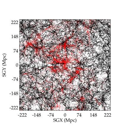
Using the halo finder, described in Aubert et al. (2004) and Tweed et al. (2009), modified to work with 2048³ ($>$2³¹) particles, dark matter halos and subhalos are detected in real space with the local maxima of dark matter particle density field. Their edge is defined as the point where the overdensity of dark matter mass drops below 80 times the background density. We further apply a lower threshold of a minimum of 100 dark matter particles. Fig. 1 shows the $\sim$40 Mpc thick XY supergalactic slice of the CLONE. Black (red) dots stand for the dark matter halos (galaxies from the 2MASS Galaxy Redshift Catalog - XSCz). Note that XSCz galaxies are used for sole comparison purposes. XSCz is indeed far more complete than the peculiar velocity catalog used to constrain the simulation ($\sim$2.5% of the redshift catalog is used to derive the peculiar velocity). In fact, it shows the constraining power of the peculiar velocities that are correlated on large scales. Namely, the simulation is constrained also in regions where no peculiar velocity measurements were available and thus used as constraints. It confirms once more that peculiar velocity catalogs fed to our technique, to reconstruct/constrain the local density and velocity fields, do not need to be complete (Sorce et al., 2017).

3 Velocity wave

Figure 2: Schema of the cylinder used to select (sub)halos whose radial peculiar velocities, derived as a function of the synthetic observer at the simulated box center, are used to study the velocity wave arisen from the massive halo in its center. While open circles stand for selected halos, dashed circles represent excluded ones.

Figure 3: Radial velocities of simulated dark matter (sub)halos (black and grey scale) and observed galaxies (orange, blue and red) as a function of the distance from the synthetic observer and us respectively. Error bars stand for uncertainties on observational distance and velocity estimates. Orange and light blue (red and dark blue) filled squares and diamonds show observed galaxies assuming H₀=74 (67.77) km s^-1 Mpc^-1 for scaling positions. CF2 (CF3) corresponds to the second (third) catalog of the Cosmicflows project. Larger symbols are used for galaxies, with a peculiar velocity higher than 1000  km s^-1, identified as the closest to the simulated massive halos assuming the synthetic observer at the box center and the same Supergalactic coordinate system and orientation as the local Universe. The arrow indicates the position of the massive dark matter halo in the simulation. Names of corresponding observed clusters are given at the top of each panel. Velocity waves stand out in the different lines-of-sight and there is a good agreement with observational datapoints for those two best-constrained clusters the closest to us. Top: Hubble diagram. Bottom: Hubble flow subtracted. The solid and dashed yellow lines are respectively the simulated positive-half velocity wave envelope and its Gaussian-plus-continuum fit. The color scale filling the black circles stands for their distance from the line-of-sight. From black to light grey, objects are less than 2.5, 5, 7.5 and 10 Mpc away from the line-of-sight. The dark matter halo virial masses in the simulation are M=9.8$\times$10¹⁴M_⊙ and M=9.0$\times$10¹⁴M_⊙ for the Virgo and Centaurus cluster counterparts respectively.

3.1 In simulated data

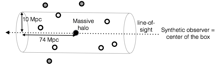
Positioning a synthetic observer at the simulation box center, we derive radial peculiar velocities for all the dark matter halos and subhalos in the z=0 catalog. We then draw lines-of-sight in the direction of each dark matter halo more massive than 5 10¹⁴M_⊙. All the (sub)halos within 10 Mpc from the line-of-sight and within 74 Mpc along the line-of-sight from a given massive dark matter halo (with the center and edge of the box as upper limits) are selected to plot the latter corresponding velocity wave. Namely, as shown on Fig. 2, radial peculiar velocities, with respect to the synthetic observer, of (sub)halos within a cylinder at maximum 148 Mpc long and 20 Mpc wide are used to visualize the velocity wave caused by the massive dark matter halo in the cylinder center. Note that because the simulation is constrained to reproduce the local Universe, we choose not to use the periodic boundary conditions to wrap around the box edges. It will indeed not be representative of local structures. A 10 Mpc radius cylinder corresponds to about three times the virial radius of the massive clusters under study here (M$>$5 10¹⁴M_⊙). Since the goal is to study the link between velocity wave properties and cluster masses, exact masses cannot be used to define the cylinder shape. Finally, such large volumes permit probing the infall region around the massive halos. Note that a cylinder shape is preferable to a cone shape to get an unbiased wave signal. A cone would indeed result in a distorted signal as it would probe a larger and larger region around a massive halo with the distance.

3.2 In observational data

Observational data are taken from the raw second and third catalogs of the Cosmicflows project (Tully et al., 2013, 2016). Note that the second catalog containing $\sim$8000 galaxies, with a mean distance of $\sim$90 Mpc, serves as the basis to build the constraint-catalog of $\sim$5000 bias-minimized radial peculiar velocities of galaxies and groups with a mean distance of $\sim$60 Mpc. By contrast, the third catalog contains $\sim$17,000 galaxies with a mean distance of $\sim$120 Mpc. The third catalog is not used to constrained our CLONE initial conditions and thus constitute partly an independent dataset for consistency check. More precisely, it serves the two-fold goal of extending the number of observational datapoints to be compared with the simulation and highlighting again the constraining power of peculiar velocities. The latter can indeed permit recovering structures that are not directly probed and that are at the limit of the non-linear threshold. In the sense that there is no direct measurement in a given region but, because the latter influences the velocities of other regions (large scale correlations), it can still be reconstructed.

Uncertainties on distances and radial peculiar velocities in these catalogs depend on the distance indicator used to derive the distance moduli. Error bar sizes need to be limited to see clearly velocity waves. Thus, to be able to compare with the simulated data, only galaxies with uncertainties on distance moduli smaller than 0.2 dex are retained. There remain 338 and 424 galaxies respectively from the second and third catalogs with a mean distance of $\sim$50 Mpc. These galaxies are mostly hosts of supernovae, especially those the furthest from us (distance indicator with a small uncertainty even as the distance increases).

To derive the radial peculiar velocities of these galaxies, we use both galaxy distance moduli ($\mu$) and observational redshifts (z_obs) following Davis & Scrimgeour (2014). We add supergalactic longitude and latitude coordinates to derive galaxy cartesian supergalactic coordinates. A cosmological model is then required to determine peculiar velocities. While we use $\Lambda$CDM, as cosmicflows catalog zero points are calibrated through a long process on WMAP (rather than Planck) values ($\Omega_{m}$=0.27, $\Omega_{\Lambda}$=0.73, H₀=74  km s^-1 Mpc^-1, Tully et al., 2013, 2016), we have to use the same parameter values. We indeed showed that when applying the bias minimization technique to the peculiar velocity catalog of constraints, we drastically reduce the dependence on $\Lambda$CDM cosmological parameter values (Sorce & Tempel, 2017). However, in order to be able to probe the whole velocity wave for the comparisons, we have to use the raw catalog i.e. with neither galaxy grouping nor bias minimization. Consequently, if were to take Planck values to derive galaxy peculiar velocities, the WMAP calibration would translate into a residual Hubble flow visible in the background-expansion-subtracted Hubble diagram. Subsequently, using WMAP values for the observations:

Luminosity distances, $d_{\mathrm{lum}}$, are derived from distance modulus measurements, $\mu$, obtained via distance indicators:

$$\mu=5\mathrm{log_{10}}(d_{\mathrm{lum}}~{}\mathrm{(Mpc)})+25$$ (1)

Cosmological redshifts, z_cos, are then obtained through the equation:

$$d_{\mathrm{lum}}=(1+z_{\mathrm{cos}})\int_{0}^{z_{\mathrm{cos}}}\frac{cdz}{H_{0}\sqrt{(1+z)^{3}\Omega_{m}+\Omega_{\Lambda}}}$$ (2)

Galaxy radial peculiar velocity, $v_{\mathrm{pec}}$, are finally estimated, using the observational z_obs and cosmological z_cos redshifts with the following formula:

$$v_{\mathrm{pec}}=c\frac{z_{\mathrm{obs}}-z_{\mathrm{cos}}}{1+z_{\mathrm{cos}}}$$ (3)

where $v_{\mathrm{pec}}$ will always refer to the radial peculiar velocity in this paper and $c$ is the speed of light.

3.3 Simulated vs. observed data

Assuming the synthetic observer at the box center and the simulated volume oriented similarly to the local volume, observed and simulated positions and lines-of-sight can be matched. We can only compare velocity waves born from local galaxy clusters for which infalling galaxy peculiar velocities, with uncertainties on corresponding distance moduli smaller than 0.2 dex, are available in the observed cluster surroundings. We thus select these clusters. For each simulated massive dark matter halo, the quickest way is then to search for the closest observed galaxy, in our selected above samples, with a radial peculiar velocity greater than 1000 km s^-1 ($\sim$2$\sigma$ above the average). This is indeed a signature that it has most probably an observed cluster with a mass of at least a few 10¹⁴M_⊙ as a neighbor. Whenever a simulated massive dark matter halo is within the 2$\sigma$ uncertainty of the observed galaxy distance, we select all the observed galaxies in the cylinder corresponding to the line-of-sight. For every case, there is indeed a massive observed cluster in the vicinity of the galaxies. More to the point, given the Supergalactic coordinates of the observed clusters and those of the simulated ones in the box, they indeed match.

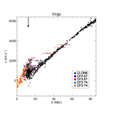
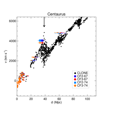
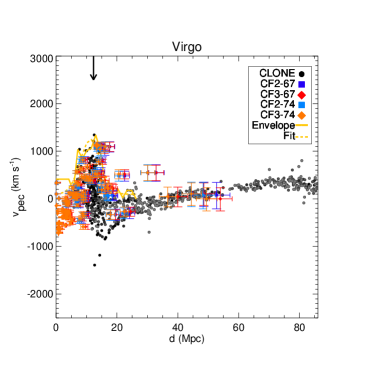
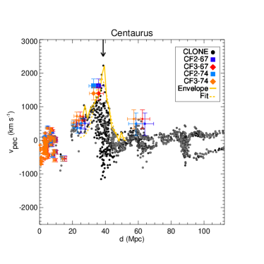
Fig. 3 superimposes observed and simulated lines-of-sight with the velocity waves born from the two closest most massive local clusters. Observational data is of sufficient quality in their respective infall region to warrant adequate comparisons. From left to right, galaxy clusters (dark matter halos) are at increasing distance from us (the synthetic observer). The name of the clusters is indicated at the top of each panel. Filled black and grey circles stand for simulated (sub)halos while filled light blue and orange squares and diamonds represent observed galaxies. Because the simulation was run with H₀ = 67.77  km s^-1 Mpc^-1, filled dark blue and red squares and diamonds are observed galaxies at positions rescaled with this latter value. Position differences are always within about the 1$\sigma$ uncertainty on the distance. Arrows indicate the position of the most massive halos in the lines-of-sight of interest.

In the top panels, the Hubble diagrams are clearly distorted by the presence of massive halos. Their corresponding velocity wave or triple-value region signatures show up. Bottom panels with the Hubble flow subtracted equally confirms the waves. The simulated velocity waves stand out in the peculiar velocity of (sub)halos plotted as a function of the distance from the synthetic observer diagrams for the two massive dark matter halos. The agreement with the observational data points is qualitatively good. All the more since only sparse peculiar velocities of today field galaxies and groups are used to constrained the linear initial density and velocity fields, at the positions of the latter progenitors, using solely linear theory and a power spectrum assuming a given cosmology. Then the full non-linear theory is used to evolved these initial conditions from the initial redshift down to z=0 within a $\Lambda$CDM framework.

The signatures of Virgo West and the group around NGC4709 that are respectively beyond Virgo and Centaurus in the lines-of-sight can also be identified as secondary waves. These smaller waves follow the highest ones representing the main clusters in both the observations and the simulation. Additionally, a void between us and Centaurus in the line-of-sight shows equally well in both the simulation and the observations. The accuracy with which the CLONE reproduces the lines-of-sight dynamical state of Virgo and Centaurus is visually excellent.

Cluster	CLONE/CF2	CLONE/CF2	CLONE/CF3	CLONE/CF3
Cylinder radius	10 Mpc	2.5 Mpc	10 Mpc	2.5 Mpc
Virgo	0.0098	0.011	0.0058	0.0071
Centaurus	0.010	0.011	0.006	0.0073
Abell 569	0.25	0.25	0.084	0.085
Coma	0.17	0.17	0.25	0.25
Abell 85	0.25	0.25	0.25	0.25
Abell 2256	0.50	0.50	0.50	0.50
PGC 765572	0.050	0.051	0.10	0.10
PGC 999654	0.50	0.50	0.50	0.50
PGC 340526	0.25	0.25	0.50	0.50
PGC 46604	0.50	0.50	0.50	0.50

Table 1: Kolmogorov-Smirnov statistic or highest distance between the cumulative distribution functions of the observed and simulated lines-of-sight including the velocity waves.

To quantify the agreement between simulated and observed lines-of-sight, we use a 2D-Kolmogorov-Smirnov statistic test applied to the simulated and observed galaxy velocity and position samples following Peacock (1983); Fasano & Franceschini (1987). p-values obtained for Virgo and Centaurus are above 0.20. They are actually close to 1.0 but values above 0.20 have no particular significance. They only confirm that the observed and simulated distributions along the line-of-sight are not significantly different. Additionally, Table 1 gives the 2D-Kolmogorov-Smirnov (KS) statistic or the highest distance between the cumulative distribution functions of the observed and simulated lines-of-sight including the velocity waves. A single 2D-KS statistic value has no particular meaning but several together permit ordering the simulated lines-of-sight from those that match the most their observational counterpart to those that match it the less (smallest to largest values). Virgo and Centaurus lines-of-sight happen to be equally well reproduced by the simulation. 2D-KS statistic values are barely different when considering all the subhalos/galaxies within a 10 Mpc radius or solely those within a 2.5 Mpc radius from the line-of-sight. The agreement is slightly better with galaxies from the third catalog (CF3) of the Cosmicflows project than with those of the second one, although the second one is the starting point to build the constrained initial conditions. However, given that the third catalog has more points and smaller uncertainties, it is encouraging that the simulation matches more the third catalog than the second one. The 2D-KS statistic test cannot indeed take into account uncertainties. Finally, 2D-KS statistic values do not differ when using H₀ = 67.77 rather than 74  km s^-1 Mpc^-1.

The 2D-KS statistic test cannot take into account the real distance of galaxies. It compares only the cumulative distributions of galaxies along the lines-of-sight using four directions (smallest to largest distances to the y-axis and vice versa, smallest to largest distances to the x-axis - in that case velocities because they are centered on zero - and vice versa). Consequently, we also define our own $\zeta$-metric to compare simulated and observed lines-of-sight as follows:

$$\zeta=\frac{1}{n}\sum^{n}_{i=1}\sqrt{(min[v_{obs}[i]-v_{sim}])^{2}+[(min[d_{obs}[i]-d_{sim}])\times H_{0}]^{2}}$$ (4)

where n is the number of observed galaxies in the line-of-sight. $v_{X}$ are the galaxy/subhalo observed and simulated peculiar velocities and $d_{X}$ are their distances.

Table 2 gives the values of $\zeta$ for the different lines-of-sight. Because $\zeta$-values are only modified by a few percent when changing H₀ value, their mean is reported in the table. Like for the 2D-KS statistic values, $\zeta$-values permit ordering the simulated lines-of-sight (including waves) that are the best reproduction of the observed ones to those that reproduce them the less. Since our $\zeta$-metric results in similar conclusions as the 2D-KS statistic does, it seems appropriate. Moreover, contrary to the 2D-KS statistic, it is sensitive to the real distance of the cluster, not solely to its position on the fraction of the line-of-sight that is studied. It thus includes both differences due to a difference in height and to a shift in position along the entire line-of-sight. It is easily checked by randomly shuffling observed and simulated lines-of-sights and comparing them. The $\zeta$-metric then gives values on average between a 100 and up to 1000 km s^-1. The $\zeta$-metric though, like the 2D-KS statistic, does not take into account uncertainties on observational distance and velocity estimates.

Cluster	CLONE/CF2	CLONE/CF2	CLONE/CF3	CLONE/CF3
Cylinder radius	10 Mpc	2.5 Mpc	10 Mpc	2.5 Mpc
Virgo	6	10	9	12
Centaurus	21	37	25	36
Abell 569	14	23	11	22
Coma	27	40	205	225
Abell 85	184	286	299	400
Abell 2256	152	152	364	364
PGC 765572	39	53	56	70
PGC 999654	687	687	662	662
PGC 340526	92	99	16	41
PGC 46604	544	544	544	544

Table 2: $\zeta$-metric in km s^-1. It measures the difference between the simulated and observed lines-of-sight. The higher $\zeta$ is the more different the lines-of-sight are. See the text for a detailed explanation.

Figure 4: Same as Figure 3 bottom panels for four clusters at increasing distance from us from left to right, top to bottom. Although these clusters are less constrained, the agreement between observed and simulated waves is still visually good especially for the first two. The dark matter halo masses in the simulation are M=9.0$\times$10¹⁴M_⊙, M=12.6$\times$10¹⁴M_⊙, M=6.6$\times$10¹⁴M_⊙ and M=11.7$\times$10¹⁴M_⊙ for Abell 569, Coma, Abell 85 and Abell 2256 cluster counterparts respectively.

In the rest of the paper, we work solely with the background expansion subtracted since it does not affect our conclusion and ease the comparisons, studies and analyses.

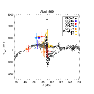
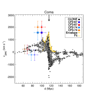
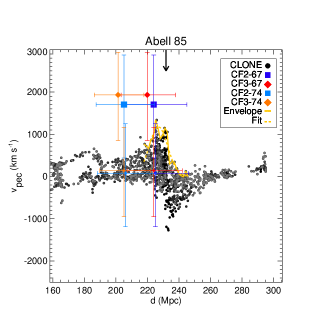
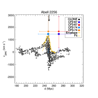
Given the above mentioned success, although the simulation matches best the local large-scale structure by construction in the inner part, where most of the constraints are, Fig. 4 shows an additional four massive halos that are more distant. These halos are still matching nicely observational clusters that are further away. Tables 1 and 2 confirm the visual impression. The different values also show the limitation of both metrics and confirm their complementarity. On the one hand, the $\zeta$-metric is more robust to small samples than the 2D-KS statistic: e.g. Abell 569 has a smaller observational sample in the second catalog of the Cosmicflows project than in the third one. However, the $\zeta$-values when comparing both observational samples to the simulated one differ by only a few percent. On the contrary, the 2D-KS statistic values grandly differ. One the other hand, the 2D-KS statistic is more robust to observational uncertainties: peculiar velocity values of galaxies in Coma, Abell 85 and Abell 2256 surroundings are compatible, given their uncertainties, between the second and third catalogs of the Cosmicflows project. They are higher though in the third catalog. Consequently, the $\zeta$-metric gives higher values when comparing lines-of-sight from this third catalog to the simulated ones rather than lines-of-sight from the second catalog to the simulated one. Note though that it is not completely unexpected that the simulated lines-of-sight match better those from the second catalog than the third one. Indeed, the second catalog is the starting point to build the constrained initial conditions.

Additionally, since observed galaxies with low distance uncertainties are usually not exactly along the line-of-sight of the massive clusters, their velocity constitutes a lower limit for the mass estimate of the observed clusters. Indeed, galaxies perfectly aligned with the observer and the cluster would have the highest possible velocity but such galaxies are difficult to distinguish from those belonging to the cluster. Consequently, for Virgo, Centaurus and Abell 569, the maximum peculiar velocity in the simulation is slightly higher than that in the observations: it confirms that the simulated cluster have reached the low mass limit set by the observations. Moreover, the difference between the observed and simulated wave maxima is small enough that masses are within the same mass range according to the Least Action modeling (see for instance Mohayaee & Tully, 2005; Tully & Mohayaee, 2004). This agreement is confirmed by observational data that follow the wave shape so as to reproduce its width. The next section expands on the link between wave properties and cluster masses. Note that the adequacy between simulated and observed velocity wave shapes is really good for Abell 569 given that even small uncertainty peculiar velocities, not used to constrain this wave progenitor in the initial conditions’ linear regime, follow also the simulated wave contour. There are indeed two orange/red datapoints from the third catalog that have no blue counterpart in the second catalog. The 2D-KS statistic small value confirms the adequacy.

Figure 5: Same as Figure 3 bottom panels for four additional clusters. Names at the top of each panel are PGC (Principal Galaxy Catalog) numbers of the galaxies with the highest velocity in the observational catalog at the given locations.

For Coma, Abell 85 and Abell 2256, given their hosted galaxy peculiar velocity uncertainties, masses are also in good agreement and the lower mass limit is reached. This is not fully expected given that these clusters are at the edge of the constrained region (50%, 90% and 99% of the constraints are in $\sim$75-80, 150-160 and 275-290 Mpc). Additional precise observational data are however required to probe the wave slopes and check their width to tighten the constraint on the masses.

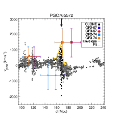
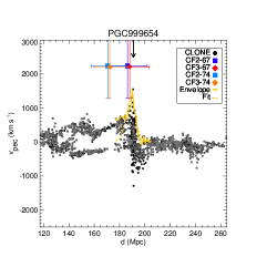
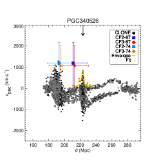
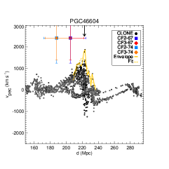
Fig. 5 shows four additional velocity waves born from massive dark matter halos to which we can associate observed galaxies. The galaxies with the largest peculiar velocities are identified by their PGC (Principal Galaxy Catalog) number at the top of each panel. Here again, given the distance of these clusters and the sparsity and limit of our constraint-catalog, the agreement is quite good. Tables 1 and 2 confirm again the visual impression. They also highlight again the limitations of both metrics. Both values must be given together to conclude on how much the observed and simulated lines-of-sight match. Note that we identify other simulated velocity waves corresponding to local clusters (e.g. in the Perseus-Pisces region) but observational data is not of sufficient quality or absent in the infall region for comparisons. Nonetheless, all the halos and associated waves are used for the next section studies. The mass range is actually extended down to 2 10¹⁴M_⊙.

4 Wave properties vs. cluster masses

4.1 The amplitude

The wave amplitude is the first obvious property to check against halo mass. Indeed, the deeper the gravitational potential well, the faster should galaxies fall onto it. The amplitude is thus defined as the difference between the maximum and minimum peculiar velocities of galaxies falling onto the cluster either from the front or from behind with respect to the synthetic observer. Fig. LABEL:fig:amplitude thus shows the amplitude of the simulated velocity waves as a function of the dark matter halo masses. Each black and red filled circle corresponds to a halo. Red ones stand for clusters identified in Fig. 3 to 5.

While it is immediate to notice that there is a clear correlation between the wave amplitude and the halo mass, one can also point out that the amplitude is extremely difficult to measure in observational data and that there is a residual scatter. Indeed, measuring the amplitude in observational data implies getting exquisite distance (peculiar velocity) estimates of galaxies exactly in the line-of-sight of the cluster with respect to us. It supposes first that there are actually galaxies exactly aligned. Then, identifying these galaxies and measuring their distances with great accuracy, while they fall onto the cluster from the front is already quite a challenge, let alone when they fall from behind.

In any case, the residual scatter suggests that the amplitude, be it measurable, alone cannot be used as a precise proxy for cluster mass estimates. Part of this scatter is probably due to the fact the galaxies are not perfectly aligned with us and the cluster. The gravitational potential well shape might also be responsible for another part of this scatter. To a lesser extent, the large-scale structure environment might also play a role.

4.2 The height

While the wave height is not expected to be a better proxy than the wave amplitude, it is interesting to check whether there still is a tight enough correlation. Indeed, while it is challenging to have precise distance measurements for both galaxies falling from the front and from behind a cluster in the line-of-sight with respect to us, it might be feasible especially for galaxies falling from the front. The height is thus defined as the maximum (minimum) peculiar velocities of galaxies falling onto the cluster from the front (behind) with respect to the synthetic observer. In Fig. LABEL:fig:height, each black and red (blue and orange) filled circles stand for the height of a dark matter halo positive-(negative-)half wave as a function of its mass. Red and orange are used for dark matter halos from Fig. 3 to 5.

A similar correlation as with the amplitude is found although with a somewhat larger scatter. Interestingly it also shows that velocity waves are not symmetric: their maximum differs from their minimum. Both the potential well shape and the non-perfect alignement observer-galaxy-halo or observer-halo-galaxy might be the reason for this asymmetry. Nonetheless because there still is a correlation and because in observational data it is easier to get accurate datapoints at the wave front than in its wake, it is legitimate to focus on the positive-half velocity wave shape to study more thoroughly the relation with the halo mass.

4.3 Height, width and continuum

After deriving the positive-half wave envelope of every dark matter halo, we choose to fit the simplest model possible, a Gaussian-plus-continuum model, to each one of them as follows:

$$v_{pec}=A_{fit}~{}\times~{}\mathrm{e}^{\frac{-(d-d_{0})^{2}}{2\sigma_{fit}^{2}}}+C_{fit}$$ (5)

where $A_{fit}$, $\sigma_{fit}$ and $C_{fit}$ are respectively the Gaussian amplitude, its standard deviation and a continuum. $d_{0}$ depends on the halo distance and has no other purpose than centering the Gaussian on zero. Its sole physical meaning is to be the actual distance of the halo. The amplitude is related to the positive-half wave envelope height while the standard deviation is linked to its width. Finally, the continuum gives the positive-half wave offset from a zero average velocity. For visualization, envelopes and their fits for halos presented in Fig. 3 to 5 are shown as solid and dashed lines on these same figures.

Fig. LABEL:fig:fits gathers the three parameters of the fits and halo masses for a concomitant study to highlight an eventual multi-parameter correlation. The Gaussian amplitude is represented as a function of the Gaussian standard deviation while the color scale stands for the continuum. From black-violet to red, the continuum decreases from positive values to negative ones. The model uncertainty is shown as error bars for the amplitude and standard deviation. The color scale smoothness includes the continuum uncertainty. The Gaussian-plus-continuum model choice proves to be robust given the tiny error bars that it results in. The filled circle sizes are proportional to the dark matter halo masses. Finally, an additional small red filled circle is used to identify each halo analyzed in Fig. 3 to 5.

The previous subsection (4.2) showed that there is a correlation between the wave height and the halo mass. It is thus not surprising to find back that the more massive the halo is (larger circle), the larger the Gaussian amplitude is (larger value). As stated above, the Gaussian amplitude is indeed the counterpart of the positive-half wave height.

In addition, there is a small correlation between the amplitude and standard deviation thus halo mass. More massive halos seem to give birth to wider waves. The scatter is however quite large. It certainly depends greatly on the halo triaxiality and thus on its orientation with respect to us. A similar conclusion is valid for the continuum, the smaller the continuum but for extreme values is, the more massive the halo is on average. Anyhow, the scatter is quite large in that case. A strong dependence on the global environment of the dark matter halo in addition to the halo mass might be in cause here.

Interestingly a general pattern emerges quite clearly though:
$\bullet$ the most massive halos ($\gtrsim$ 6 10¹⁴ M_⊙) tend to give birth to positive-half waves that have a continuum compatible with zero or slightly negative/positive in addition to high amplitude and standard deviation values.
$\bullet$ the less massive halos ( 2 10¹⁴ M_⊙$\lesssim$M$\lesssim$ 4 10¹⁴ M_⊙) tend to give birth to positive-half waves that have a continuum compatible with zero or slightly negative/positive in addition to low amplitude and standard deviation values.
$\bullet$ intermediate mass halos (4 10¹⁴ M_⊙$\lesssim$M$\lesssim$ 6 10¹⁴ M_⊙) give rise to positive-half waves that have high continuum absolute values. Such values permit distinguishing them from the most massive halos with which they share high amplitude and possibly standard deviation values, especially in the negative continuum case.
It is highly probable that the global environment or cosmic web is responsible for such a finding. We will investigate this link in more details in future studies.

The halo segregation in different continuum value classes is another quite inspiring source. There seems to be a different correlation for each continuum value class:
$\bullet$ Halos with fits resulting in a high (close to zero) continuum value seems to have masses correlated with the Gaussian amplitudes but not so much with the Gaussian standard deviations that appear to have low values (present a large scatter).
$\bullet$ Halos with fits resulting in a very low continuum value have both amplitudes and standard deviations correlated together as well as with the masses.
$\bullet$ Halos with fits resulting in either positive or negative intermediate continuum values present masses correlated with amplitudes and up to a certain point with standard deviations. Consequently, although to a lesser extent than for halos whose continuum values are quite low, amplitudes and standard deviations are slightly correlated.

To summarize, since the fit parameters are interdependent, a global fit to the velocity wave seems the best approach to obtain cluster rough mass estimates rather than single and independent measurements of amplitude, height and width. Because different categories appear among halos, in future studies, a machine learning approach might become handy to actually get accurate enough mass estimates from sparse observations. In a first approach, the simple Gaussian-plus-continuum fit presented here could be used as a model reduction.

5 Conclusions

Galaxy clusters are excellent cosmological probes provided their mass estimates are accurately determined. Fueled with large imaging surveys, stacked weak lensing is the most promising mass estimate method though it provides estimates within relatively small radii. Given the large amount of accompanying redshift and spectroscopic data overlapping the imaging surveys, we must take the opportunity to calibrate also with a reasonable accuracy a method based on galaxy dynamics. Two independent measures hold indeed better constraints on the cosmological model. Infall zones of galaxy clusters are probably the less sensitive to baryonic physics, thus mostly shielded from challenging systematics, and probe large radii. These manifestations of a tug of war between gravity and dark energy provide a unique avenue to test modified gravity theories when comparing resulting mass estimates to those from stacked weak lensing measurements. Combined with stacked weak lensing results, they might even yield evidence that departure from General Relativity on cosmological scales is responsible for the expansion acceleration.

The accurate calibration of the relation between infall zones properties and cluster masses starts with careful comparisons between cosmological simulations and observations. In this paper, we thus present our largest and highest resolution Constrained Local & Nesting Environment Simulation (CLONE) built so far to reproduce numerically our cosmic environment. This simulation stems from initial conditions constrained by peculiar velocities of local galaxies. By introducing this cosmological dark matter CLONE of the local large-scale structure with a particle mass of $\sim$10⁹M_⊙ within a $\sim$738 Mpc box, we have sufficient resolution to study the effect of the gravitational potential of massive local halos onto the velocity of (sub)halos. We can also compare with that of their observational cluster counterparts.

Velocity waves stand out in radial peculiar velocity - distance to a box-centered synthetic observer diagram. The agreement between lines-of-sight including velocity waves, caused by the most massive dark matter halos of the CLONE and those born from their observational local cluster counterparts, is visually good especially for the clusters the closest to us that are the best constrained (e.g. Virgo, Centaurus). Secondary waves due to smaller groups in (quasi) the same line-of-sight as the most massive clusters stand out equally even though they are further into the non-linear regime. Indeed, prior to full non-linear evolution to the z=0 state, assuming $\Lambda$CDM, CLONE initial conditions are constrained with solely the linear theory, a power spectrum and highly uncertain and sparse local peculiar velocities. The visual matching between the simulated and observed lines-of-sight is confirmed with 2D-Kolmogorov Smirnov (KS) statistic values and tests as well as with our own $\zeta$-metric. Contrary to the 2D-KS statistic, the $\zeta$-metric takes into account the real distance of galaxies along the entire lines-of-sight (not only the studied fractions). The $\zeta$-metric is however more sensitive to the fact that observational uncertainties are not taken into account in these metrics. The two metrics appear to be complementary. They show that the closest clusters have the best reproduced lines-of-sight. The lines-of-sight of clusters at the edges of the constrained region and even slightly beyond are also reproduced by the simulation although to a smaller extent.

Additionally, a Gaussian-plus-continuum fit to the envelope of the positive-half of all the velocity waves born from dark matter halos more massive than 2 10¹⁴M_⊙ in the simulation reveals both the variety and complexity of the potential wells as well as the correlation of the fit parameters with the halo masses. Overall, the Gaussian amplitude is mostly linked to the halo mass, but for a few exceptions, with a residual scatter. Although the Gaussian standard deviation is not always correlated with the mass, it can be slightly correlated with the Gaussian amplitude thus with the mass. The continuum is certainly an interesting parameter to consider as it permits splitting the halos into different classes. Each continuum value seems to drive a given correlation between the Gaussian amplitude and the halo mass and, to a smaller extent, with the Gaussian standard deviation. To summarize, parameter fits are completely interdependent, a global fit to the velocity wave is then the best approach to obtain a first rough cluster mass estimate.

First and foremost, this work confirms the potential of the velocity wave technique to get massive cluster mass estimates and test gravity and cosmological models. Our CLONES, with the first shown reproduction of observed lines-of-sight including velocity waves, could in the near future provide the zero point of galaxy infall kinematic technique calibrations (Zu & Weinberg, 2013). A bayesian inference model or/and a machine learning technique built and trained on random simulated galaxy surveys that is then applied to both constrained simulated and observed galaxy surveys must recover the same local velocity waves and corresponding mass estimates to be validated. Our CLONES will moreover allow minimizing observational biases as any real environmental and cluster property will be reproduced for perfect one-to-one comparisons. Local kinematic mass estimates can then become accurate. Once compared with other techniques of local galaxy cluster mass estimates, they will permit calibrating the zero-point of these other techniques to be applied to further-and-further away clusters.

Data availability

Synthetic catalogs are available upon reasonable request to the authors.

References

- Aubert et al. (2004) Aubert D., Pichon C., Colombi S., 2004, MNRAS, 352, 376
- Burke (2006) Burke D., 2006, in APS April Meeting Abstracts
- Carlberg et al. (1997) Carlberg R. G. et al., 1997, ApJ, 485, L13
- Cirasuolo et al. (2014) Cirasuolo M. et al., 2014, in Society of Photo-Optical Instrumentation Engineers (SPIE) Conference Series, Vol. 9147, Ground-based and Airborne Instrumentation for Astronomy V, Ramsay S. K., McLean I. S., Takami H., eds., p. 91470N
- Davis & Scrimgeour (2014) Davis T. M., Scrimgeour M. I., 2014, MNRAS, 442, 1117
- de Jong et al. (2012) de Jong R. S. et al., 2012, in Society of Photo-Optical Instrumentation Engineers (SPIE) Conference Series, Vol. 8446, Ground-based and Airborne Instrumentation for Astronomy IV, McLean I. S., Ramsay S. K., Takami H., eds., p. 84460T
- Diaferio (1999) Diaferio A., 1999, MNRAS, 309, 610
- Fasano & Franceschini (1987) Fasano G., Franceschini A., 1987, MNRAS, 225, 155
- Gottlöber et al. (2010) Gottlöber S., Hoffman Y., Yepes G., 2010, ArXiv e-prints: 1005.2687
- Green et al. (2012) Green J. et al., 2012, arXiv e-prints, arXiv:1208.4012
- Heisler et al. (1985) Heisler J., Tremaine S., Bahcall J. N., 1985, ApJ, 298, 8
- Jasche & Wandelt (2013) Jasche J., Wandelt B. D., 2013, MNRAS, 432, 894
- Karachentsev & Nasonova (2013) Karachentsev I. D., Nasonova O. G., 2013, MNRAS, 429, 2677
- Karachentsev et al. (2013) Karachentsev I. D., Nasonova O. G., Courtois H. M., 2013, MNRAS, 429, 2264
- Kitaura (2013) Kitaura F.-S., 2013, MNRAS, 429, L84
- Kravtsov & Borgani (2012) Kravtsov A. V., Borgani S., 2012, ARA&A, 50, 353
- Mandelbaum et al. (2006) Mandelbaum R., Seljak U., Cool R. J., Blanton M., Hirata C. M., Brinkmann J., 2006, MNRAS, 372, 758
- Mohayaee & Tully (2005) Mohayaee R., Tully R. B., 2005, ApJ, 635, L113
- Olchanski & Sorce (2018) Olchanski M., Sorce J. G., 2018, A&A, 614, A102
- Peacock (2008) Peacock J., 2008, in A Decade of Dark Energy
- Peacock (1983) Peacock J. A., 1983, MNRAS, 202, 615
- Planck Collaboration et al. (2014) Planck Collaboration et al., 2014, A&A, 571, A16
- Planck Collaboration et al. (2016) Planck Collaboration et al., 2016, A&A, 594, A24
- Pratt et al. (2019) Pratt G. W., Arnaud M., Biviano A., Eckert D., Ettori S., Nagai D., Okabe N., Reiprich T. H., 2019, Space Sci. Rev., 215, 25
- Sorce (2015) Sorce J. G., 2015, MNRAS, 450, 2644
- Sorce (2018) Sorce J. G., 2018, MNRAS, 478, 5199
- Sorce et al. (2019) Sorce J. G., Blaizot J., Dubois Y., 2019, MNRAS, 486, 3951
- Sorce et al. (2021) Sorce J. G., Dubois Y., Blaizot J., McGee S. L., Yepes G., Knebe A., 2021, MNRAS, 504, 2998
- Sorce et al. (2016a) Sorce J. G., Gottlöber S., Hoffman Y., Yepes G., 2016a, MNRAS, 460, 2015
- Sorce et al. (2016b) Sorce J. G. et al., 2016b, MNRAS, 455, 2078
- Sorce et al. (2017) Sorce J. G., Hoffman Y., Gottlöber S., 2017, MNRAS, 468, 1812
- Sorce & Tempel (2017) Sorce J. G., Tempel E., 2017, MNRAS, 469, 2859
- Sorce & Tempel (2018) Sorce J. G., Tempel E., 2018, MNRAS, 476, 4362
- Teyssier (2002) Teyssier R., 2002, A&A, 385, 337
- Tonry & Davis (1981) Tonry J. L., Davis M., 1981, ApJ, 246, 680
- Tully (2015) Tully R. B., 2015, AJ, 149, 54
- Tully et al. (2013) Tully R. B. et al., 2013, AJ, 146, 86
- Tully et al. (2016) Tully R. B., Courtois H. M., Sorce J. G., 2016, AJ, 152, 50
- Tully & Mohayaee (2004) Tully R. B., Mohayaee R., 2004, in IAU Colloq. 195: Outskirts of Galaxy Clusters: Intense Life in the Suburbs, Diaferio A., ed., pp. 205–211
- Tweed et al. (2009) Tweed D., Devriendt J., Blaizot J., Colombi S., Slyz A., 2009, A&A, 506, 647
- Weinberg et al. (2013) Weinberg D. H., Mortonson M. J., Eisenstein D. J., Hirata C., Riess A. G., Rozo E., 2013, Phys. Rep., 530, 87
- Zu & Weinberg (2013) Zu Y., Weinberg D. H., 2013, MNRAS, 431, 3319
- Zu et al. (2014) Zu Y., Weinberg D. H., Jennings E., Li B., Wyman M., 2014, MNRAS, 445, 1885