Spatially quasi-periodic water waves of finite depth

Abstract.

We present a numerical study of spatially quasi-periodic gravity-capillary waves of finite depth in both the initial value problem and traveling wave settings. We adopt a quasi-periodic conformal mapping formulation of the Euler equations, where one-dimensional quasi-periodic functions are represented by periodic functions on a higher-dimensional torus. We compute the time evolution of free surface waves in the presence of a background flow and a quasi-periodic bottom boundary and observe the formation of quasi-periodic patterns on the free surface. Two types of quasi-periodic traveling waves are computed: small-amplitude waves bifurcating from the zero-amplitude solution and larger-amplitude waves bifurcating from finite-amplitude periodic traveling waves. We derive weakly nonlinear approximations of the first type and investigate the associated small-divisor problem. We find that waves of the second type exhibit striking nonlinear behavior, e.g., the peaks and troughs are shifted non-periodically from the corresponding periodic waves due to the activation of quasi-periodic modes.

1. Introduction

Free surface waves on incompressible fluids arise in many contexts in fluid dynamics. Examples include ocean wave forecasting [36, 60], modeling the motion of flows over obstacles and varying bottom boundaries [66, 28, 5], and studying wind-wave interactions in extreme wave events, such as freak waves [38]. These models are described by the Euler equations, which are usually studied under periodic boundary conditions or the assumption that solutions decay to zero at infinity [37, 4, 32]. However, these assumptions are insufficient in many problems of interest. For instance, a periodic wave could interact with a bottom boundary with a different spatial period, or subharmonic perturbations of a periodic traveling wave can grow in amplitude, leading to quasi-periodic waves. To tackle these issues, we recently proposed methods [72, 73] to study the Euler equations under quasi-periodic boundary conditions; specifically, we studied spatially quasi-periodic waves of infinite depth in two dimensions and developed numerical algorithms to compute such waves. In this paper, we extend this previous work to the finite-depth case and discuss both the initial value and traveling wave problems in the quasi-periodic setting.

Finite-depth water waves exhibit interesting nonlinear dynamics. It has been shown numerically that Fermi-Pasta-Ulam recurrence can occur in free surface waves of finite depth when the wave amplitude is less than about $1/10$ of the fluid depth [57, 55]. A varying bottom boundary can lead to substantial amplifications of water waves. There have been both experimental and numerical studies demonstrating increased freak wave activities when waves propagate over a sloping bottom, from a deeper to a shallower domain [63, 20]. In the problem of long waves approaching vertical walls, an abrupt transition in the bottom boundary can cause large runups on the wall or wave breaking, which generally occurs when the wave crest overturns [65, 33]. The interaction between a rotational wave current and a varying bottom boundary gives rise to a time-dependent Kelvin cat-eye structure [28].

The quasi-periodic dynamics of water waves have recently drawn considerable attention. Berti and Montalto [9], Baldi et al. [6], Berti et al. [8, 7], and Feola and Giuliani [26] have used Nash-Moser theory to prove the existence of small-amplitude temporally quasi-periodic water waves. On the numerical side, Wilkening computed new families of relative-periodic [69] and traveling-standing [70] water waves. Although the physical mechanisms are different, temporally and spatially quasi-periodic waves have similar mathematical structures in that they can both be formulated in terms of periodic functions on a higher-dimensional torus. Damanik and Goldstein [17] proved the global existence and uniqueness of small-amplitude spatially quasi-periodic solutions of the KdV equation. Oh [49] and Dodson et al. [19] showed the local existence of spatially quasi-periodic solutions of nonlinear Schrödinger equations.

We were originally motivated by the structure of quasi-crystals in material science. Blinov [10] used quasi-periodic solutions of the Schrödinger equation to describe the electronic structure of non-interacting electrons in a quasi-crystals. To study how electrons move through quasi-crystals, Torres et al. [61] created quasi-periodic standing waves by vibrating a fluid-filled pan with a quasi-periodic bottom boundary and sent a transverse wave pulse across the fluid that develops a non-periodic pattern in which the spacing between the wave peaks is not constant. Their observation inspired us to ask the following question: how do we compute the exact dynamics of free surface waves in the presence of a quasi-periodic bottom boundary? To address this question, one needs to study the free surface wave problem in a quasi-periodic framework.

Another reason for our interest in quasi-periodic water waves originates from the dispersion relation of gravity-capillary waves of finite depth:

(1.1) $$c^{2}=(gk^{-1}+\tau k)\tanh(kh).$$

Here $c$ is the phase speed, $k$ is the wave number, $g$ is the acceleration due to gravity, $\tau$ is the coefficient of surface tension and $h$ is the depth of the fluid. It is known [62] that when $\tau/(gh^{2})<1/3$, there exists $c_{\text{crit}}$ between 0 and $\sqrt{gh}$ such that for any fixed phase speed $c>c_{\text{crit}}$, there are two distinct positive wave numbers satisfying the dispersion relation (1.1), which we denote by $k_{1}$ and $k_{2}$. Any superposition of waves with these two wave numbers is a solution of the linearized traveling wave problem. If $k_{1}$ and $k_{2}$ are rationally related, the linear solution is spatially periodic and related to the well-studied Wilton ripples [75, 62, 2, 1]. On the other hand, if $k_{1}$ and $k_{2}$ are irrationally related, the linear solution will be spatially quasi-periodic, which gives a natural place to search for nonlinear quasi-periodic traveling solutions. Bridges and Dias [13] first studied these spatially quasi-periodic traveling waves using a spatial Hamiltonian structure and constructed weakly nonlinear approximations of these waves. Recently, we [72] used a conformal mapping formulation of the water wave equations and computed highly accurate numerical solutions of the fully nonlinear problem in the case of deep water. These computations are performed on a two-dimensional torus from which we extract 1D quasi-periodic functions via $u(\alpha)=\tilde{u}(k_{1}\alpha,k_{2}\alpha)$. The computational challenges are similar to those of computing time-periodic standing waves [42, 68, 71]. The main difference is that standing waves can be formulated as a nonlinear two-point boundary value problem, which reduces the number of unknowns from $O(N^{2})$ to $O(N)$ initial degrees of freedom, while quasi-periodic traveling waves have $O(N^{2})$ unknowns but a simpler objective function whose main cost is the relatively inexpensive two-dimensional FFT. In the present work, we aim to further extend these techniques to the case of finite-depth water.

Following [72, 73], we adopt a conformal mapping formulation of the free surface Euler equations [22, 23, 15, 21, 77, 40, 34, 24]. In the finite depth case, the fluid domain with a curved surface and an uneven bottom boundary is mapped conformally onto a horizontal strip instead of the lower half-plane. Since the conformal mapping depends on time, even though the bottom boundary is fixed in physical space, the representation of the bottom boundary in conformal space varies with time. Ruban [54, 56] fixed the width of the strip and used a composition of two conformal mappings to map the strip to the fluid domain – the first leaves the real axis invariant and the second maps the real line to the bottom boundary. Viotti et al. [66], Flamarion et al. [29, 27] and Ribeiro et al. [53] let the width of the strip vary with time to keep the wave length the same in physical space and conformal space. They used a fixed-point iterative method to compute the bottom profile at different times. In order that water waves possess the same quasi-periods in both physical and conformal spaces, we also let the strip width be a time-dependent variable. However, in contrast to [66, 29], we compute the time evolution of the bottom profile directly, employing analytical properties of the conformal mapping, similar to [54, 56]. As in the infinite-depth case [73, 72], we introduce finite-depth quasi-periodic Hilbert transforms to relate the real and imaginary parts of the conformal mapping and to compute the kinematic boundary condition on the free surface. These Hilbert transforms are Fourier multiplier operators and are easier to compute in a quasi-periodic setting than a more direct computation of the Dirichlet-Neumann operator [16] in physical space, e.g., using boundary integral methods [5].

In computing the dynamics of free surface waves over a varying bottom boundary, it is usually assumed that the spatial periods of the free surface wave and the bottom boundary are the same or one is an integer multiple of the other. In this paper, we study a new situation where their spatial periods are irrationally related. Specifically, in one of the examples presented in Section 4.1, we compute the time evolution of an initially periodic free surface wave with period $2\pi$ in the presence of a periodic bottom boundary with period $2\sqrt{2}\pi$. We find that the periodic wave becomes a quasi-periodic wave, with each wave peak and trough evolving differently as it interacts with the bottom boundary. We also compute the time evolution of an initially flat free surface in the presence of a background flow and a quasi-periodic bottom boundary. Similar to the experiment by Torres et al. [61], we also observe that the free surface wave develops quasi-periodic patterns as a result of interactions between the background flow and the quasi-periodic bottom boundary. The wave peaks and troughs are asymmetric and the distance between adjacent wave peaks is not constant.

In Section 4.2, we compute two types of quasi-periodic traveling solutions: waves that bifurcate from the zero-amplitude solution and waves that bifurcate from finite-amplitude periodic traveling solutions. For the first type, we use linearization about the zero solution for the initial bifurcation direction and obtain a three-parameter family of solutions prescribed by the fluid depth and Fourier coefficients corresponding to wave numbers $k_{1}$ and $k_{2}$; these are called the base Fourier coefficients. Similar to the case of deep water [72], when the amplitudes of the base Fourier coefficients are small, the solutions are of small amplitude and are close to the linear solution. For the second type, we linearize the governing equations around a finite-amplitude $2\pi$-periodic traveling wave. For the bifurcation direction in this case, we use a quasi-periodic function of the following form in the kernel of the linear operator:

(1.2) $$\delta\eta(\alpha)=e^{ik\alpha}\eta_{0}(\alpha)+c.c.,$$

where $\eta_{0}$ possesses the same wavelength as the periodic traveling wave, the notation $c.c.$ denotes the complex conjugate of the preceding term, and we set $k=1/\sqrt{2}$ in this paper. This method has also been used to compute secondary periodic bifurcations with $k=1/2$ and $k=1/3$ by Chen and Saffman [14] and with $k=1/9$ by Vanden-Broeck [64]. In the present work, we obtain quasi-periodic traveling waves that bifurcate from a periodic traveling wave whose first Fourier mode resonates with the fifth Fourier mode. The periodic traveling wave is a solution of the Wilton ripple problem and the wave peaks look like “cat ears”. The bifurcated wave still preserves this characteristic; however, influenced by the Fourier modes in the quasi-periodic direction, the distance between the successive “ears” is no longer constant.

The paper is organized as follows. In Section 2, we define finite-depth quasi-periodic Hilbert transforms and derive equations of motion for quasi-periodic free surface waves in conformal space when the bottom boundary is not necessarily flat. In Section 3, we obtain the governing equations of quasi-periodic traveling waves in the case of finite-depth water with a flat bottom boundary and establish weakly nonlinear approximations of these waves and the role of small divisors in computing successive approximations. In Section  4, we use a Fourier pseudo-spectral method to compute solutions of the initial value and traveling wave problems and present various numerical examples. Following the idea in [73, 72], we lift the one-dimensional quasi-periodic problem to a higher-dimensional periodic torus where the computation is performed. We formulate the traveling wave problem as an overdetermined nonlinear least-squares problem that we solve through a variant of the Levenberg-Marquardt method [48, 71]. For the initial value problem, we consider the natural setting where the quasi-periodic initial condition and bottom boundary are posed in physical space. We present a method of transforming them to conformal space in Appendix A.

2. Equations of motion

2.1. Governing equations in physical space

Gravity-capillary waves of finite depth are governed by the free-surface Euler equations [76, 37]. In two dimensions, they may be written as

(2.1) $$\eta^{\text{s}}(x,0)=\eta^{\text{s}}_{0}(x),\qquad\varphi(x,0)=\varphi_{0}(x),\qquad t=0,\quad x\in\mathbb{R},$$

(2.2) $$\Phi_{xx}+\Phi_{yy} =0, \qquad\qquad\eta^{\text{b}}(x) <y<\eta^{\text{s}}(x,t),$$

$$\Phi =\varphi, \qquad\qquad y =\eta^{\text{s}}(x,t),$$

$$\nabla\Phi\cdot\boldsymbol{n} =0, \qquad\qquad y =\eta^{\text{b}}(x),$$

(2.3) $$\eta^{\text{s}}_{t}=\Phi_{y}-\eta^{\text{s}}_{x}\Phi_{x},\qquad\qquad y=\eta^{\text{s}}(x,t),$$

(2.4) $$\varphi_{t}=\Phi_{y}\eta^{\text{s}}_{t}-\frac{1}{2}\Phi_{x}^{2}-\frac{1}{2}\Phi_{y}^{2}-g\eta^{\text{s}}+\tau\frac{\eta_{xx}^{\text{s}}}{\big{(}1+(\eta_{x}^{\text{s}})^{2}\big{)}^{3/2}}+C(t),\qquad y=\eta^{\text{s}}(x,t),$$

where $x$ is the horizontal coordinate, $y$ is the vertical coordinate, $t$ is the time, $\Phi(x,y,t)$ is the velocity potential of the fluid, $\eta^{\text{s}}(x,t)$ is the free surface elevation, $\eta^{\text{b}}(x)$ is the fixed bottom profile, $g$ is the vertical acceleration due to gravity, and $\tau$ is the coefficient of surface tension, which is zero for gravity waves. Equation (2.3) is the kinematic boundary condition and (2.4) is the dynamic boundary condition. The function $C(t)$ in (2.4) is an arbitrary integration constant that is allowed to depend on time but not space. We are interested in the dynamics of the water waves in the presence of a varying bottom boundary; in other words, the bottom profile is not a constant function. When the bottom boundary is flat, it is usually assumed that there is no background flow. Indeed, in this case, the system is Galilean invariant, which means any background flow can be eliminated by viewing the system in a moving frame. However, this is not true when the bottom boundary is variable; the interaction between the background flow and the bottom boundary can lead to interesting nonlinear dynamics. Therefore, it is meaningful to incorporate a background flow in the problem description by including a secular growth term in the velocity potential, which is otherwise spatially periodic or quasi-periodic.

2.2. Finite-depth quasi-periodic Hilbert transforms

As defined in [44, 25], a quasi-periodic, real-analytic function $f(\alpha)$ is a function of the form

(2.5) $$f(\alpha)=\tilde{f}(\boldsymbol{k}\alpha),\qquad\tilde{f}(\boldsymbol{\alpha})=\sum_{\boldsymbol{j}\in\mathbb{Z}^{d}}\hat{f}_{\boldsymbol{j}}e^{i\langle\boldsymbol{j},\,\boldsymbol{\alpha}\rangle},\qquad\alpha\in\mathbb{R},\;\;\boldsymbol{\alpha},\boldsymbol{k}\in\mathbb{R}^{d},$$

where $\langle\cdot,\,\cdot\rangle$ denotes the standard inner product on $\mathbb{R}^{d}$ and $\tilde{f}$ is a periodic, real-analytic function defined on the $d$-dimensional torus $\mathbb{T}^{d}:=\mathbb{R}^{d}\big{/}(2\pi\mathbb{Z})^{d}.$ We assume that $d\geq 2$ so that $f$ can be genuinely quasi-periodic. Entries of the vector $\boldsymbol{k}$ are called the basic wave numbers (or basic frequencies) of $f$ and are required to be linearly independent over $\mathbb{Z}$. Given a quasi-periodic function $f$, the corresponding $\tilde{f}$ and $\boldsymbol{k}$ in (2.5) are not unique. Indeed, if $\boldsymbol{K}$ is any $d$-by-$d$ unimodular matrix, then $\tilde{f}^{\prime}(\boldsymbol{\alpha})=\tilde{f}(\boldsymbol{K}\boldsymbol{\alpha})$ also satisfies (2.5) with $\boldsymbol{k}^{\prime}=\boldsymbol{K}^{-1}\boldsymbol{k}$. For simplicity, we assume $\boldsymbol{k}$ is given, along with $f$ or $\tilde{f}$, to pin down the representation. Given $\boldsymbol{k}$, one can reconstruct $\tilde{f}$ and its Fourier coefficients $\hat{f}_{\boldsymbol{j}}$ from $f$ via

(2.6) $$\hat{f}_{\boldsymbol{j}}=\lim_{a\to\infty}\frac{1}{2a}\int_{-a}^{a}f(\alpha)e^{-i\langle\boldsymbol{j},\boldsymbol{k}\rangle\alpha}d\alpha,\qquad\boldsymbol{j}\in\mathbb{Z}^{d}.$$

We refer to [11] for detailed discussions of the above averaging formula. We assume that $\tilde{f}(\boldsymbol{\alpha})$ is real-analytic, which is equivalent to the conditions that $\hat{f}_{-\boldsymbol{j}}=\overline{\hat{f}_{\boldsymbol{j}}}$ for $\boldsymbol{j}\in\mathbb{Z}^{d}$ and there exist positive numbers $M$ and $\gamma$ such that $|\hat{f}_{\boldsymbol{j}}|\leq Me^{-\gamma\|\boldsymbol{j}\|}$, i.e., the Fourier modes $\hat{f}_{\boldsymbol{j}}$ decay exponentially as $\|\boldsymbol{j}\|\rightarrow\infty$. Next we introduce some operators that act on $f$ and $\tilde{f}$.

Definition 2.1.

The projection operators $P$ and $P_{0}$ are defined by

(2.7) $$P=\operatorname{id}-P_{0},\qquad P_{0}[f]=P_{0}[\tilde{f}]=\hat{f}_{\boldsymbol{0}}=\frac{1}{(2\pi)^{d}}\int_{\mathbb{T}^{d}}\tilde{f}(\boldsymbol{\alpha})\,d\alpha_{1}\cdots\,d\alpha_{d}.$$

Note that $P$ projects onto the space of zero-mean functions and $P_{0}$ returns the mean value. There are two versions of $P$ and $P_{0}$, one acting on quasi-periodic functions defined on $\mathbb{R}$ and one acting on torus functions defined on $\mathbb{T}^{d}$.

Definition 2.2.

The derivative operator $\partial_{\alpha}$ that acts on $f$ or $\tilde{f}$ is defined by

(2.8) $$\partial_{\alpha}f(\alpha)=\partial_{\alpha}\tilde{f}(\boldsymbol{k}\alpha),\qquad\partial_{\alpha}\tilde{f}(\boldsymbol{\alpha})=\sum_{\boldsymbol{j}\neq\boldsymbol{0}}i\langle\boldsymbol{j},\boldsymbol{k}\rangle\hat{f}_{\boldsymbol{j}}e^{i\langle\boldsymbol{j},\boldsymbol{\alpha}\rangle}.$$

For simplicity of notation, we denote $\partial_{\alpha}f$ (or $\partial_{\alpha}\tilde{f}$) by $f_{\alpha}$ (or $\tilde{f}_{\alpha}$). One can also interpret $\partial_{\alpha}\tilde{f}$ as the directional derivative of $\tilde{f}$ along the characteristic direction $\boldsymbol{k}$.

Definition 2.3.

We introduce four finite-depth quasi-periodic Hilbert transforms $H^{\tanh}$, $H^{\coth}$, $H^{\operatorname{csch}}$, $H^{\operatorname{sech}}$ that act on $f$ and $\tilde{f}$ as follows [51, 66]

(2.9) $$H^{\operatorname{op}}[f](\alpha)=H^{\operatorname{op}}[\tilde{f}](\boldsymbol{k}\alpha),\qquad H^{\operatorname{op}}[\tilde{f}](\boldsymbol{\alpha})=\sum_{\boldsymbol{j}\in\mathbb{Z}^{d}}i\hat{H}^{\operatorname{op}}\hat{f}_{\boldsymbol{j}}e^{i\langle\boldsymbol{j},\boldsymbol{\alpha}\rangle},$$

where $\operatorname{op}=\tanh,\coth,\operatorname{sech}$ or $\operatorname{csch}$ and the symbol $\hat{H}^{\operatorname{op}}$ is given by

(2.10) $$\hat{H}_{\boldsymbol{j}}^{\tanh} =i\tanh\big{(}\langle\boldsymbol{j},\boldsymbol{k}\rangle h\big{)}, \qquad\hat{H}_{\boldsymbol{j}}^{\coth} =\begin{cases}(-i)\coth\big{(}\langle\boldsymbol{j},\boldsymbol{k}\rangle h\big{)},&\boldsymbol{j}\neq\boldsymbol{0},\\ 0&\boldsymbol{j}=\boldsymbol{0},\end{cases}$$

$$\hat{H}_{\boldsymbol{j}}^{\operatorname{sech}} =\operatorname{sech}\big{(}\langle\boldsymbol{j},\boldsymbol{k}\rangle h\big{)}, \qquad\hat{H}_{\boldsymbol{j}}^{\operatorname{csch}} =\begin{cases}i\operatorname{csch}\big{(}\langle\boldsymbol{j},\boldsymbol{k}\rangle h\big{)}&\boldsymbol{j}\neq\boldsymbol{0},\\ 0&\boldsymbol{j}=\boldsymbol{0}.\end{cases}$$

Here $h$ is a positive parameter that will be discussed in Section 2.3.

We notice that

(2.11) $$\lim_{h\to\infty}\hat{H}_{\boldsymbol{j}}^{\tanh}=i\operatorname{sgn}\big{(}\langle\boldsymbol{j},\boldsymbol{k}\rangle\big{)},\qquad\qquad\lim_{h\to\infty}\hat{H}_{\boldsymbol{j}}^{\coth}=-i\operatorname{sgn}\big{(}\langle\boldsymbol{j},\boldsymbol{k}\rangle\big{)}.$$

The latter coincides with the quasi-periodic Hilbert transform introduced in [73, 72] in the case of deep water while the former is its pseudo-inverse.

2.3. The quasi-periodic conformal mapping

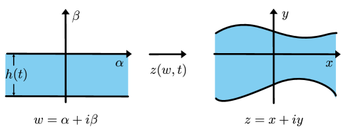
Figure 1. The time-dependent conformal mapping.

Figure 1 illustrates a time-dependent conformal mapping

(2.12) $$z(w,t)=x(\alpha,\beta,t)+iy(\alpha,\beta,t),\qquad\qquad w=\alpha+i\beta,$$

that maps the infinite strip in the complex plane

(2.13) $$S_{h}=\{\alpha+i\beta\,:\,\alpha\in\mathbb{R},\,-h(t)<\beta<0\}$$

to the fluid domain

(2.14) $$\Omega_{f}=\{(x,y)\,:\,x\in\mathbb{R},\,\eta^{\text{b},\text{phys}}(x)<y<\eta^{\text{s},\text{phys}}(x,t)\}.$$

To avoid ambiguity, we use $\eta^{\text{s},\text{phys}}$ and $\eta^{\text{b},\text{phys}}$ to denote the free surface elevation and the bottom profile in physical space, respectively, whereas $\eta^{\text{s}}$ and $\eta^{\text{b}}$ are used as conformal variables henceforth.

We assume that $z(w,t)$ can be extended continuously to $\overline{S_{h}}$ and maps the top and bottom boundary of the strip to the free surface and the bottom boundary of the fluid domain, respectively. Denoting

(2.15) $$\zeta^{\text{s}}(\alpha,t) =z|_{\beta=0}(\alpha,t)=x(\alpha,0,t)+iy(\alpha,0,t)=\xi^{\text{s}}(\alpha,t)+i\eta^{\text{s}}(\alpha,t),$$

$$\zeta^{\text{b}}(\alpha,t) =z|_{\beta=-h(t)}(\alpha,t)=x(\alpha,-h(t),t)+iy(\alpha,-h(t),t)=\xi^{\text{b}}(\alpha,t)+i\eta^{\text{b}}(\alpha,t),$$

we have

(2.16) $$\eta^{\text{s},\text{phys}}(\xi^{\text{s}}(\alpha,t),t)=\eta^{\text{s}}(\alpha,t),\qquad\qquad\eta^{\text{b},\text{phys}}(\xi^{\text{b}}(\alpha,t))=\eta^{\text{b}}(\alpha,t).$$

For later use in the derivation of the governing equations in conformal space, we compute the derivative with respect to $\alpha$ and $t$ on both sides of (2.15) and obtain that

(2.17) $$x_{\alpha}=\xi^{\text{s}}_{\alpha},\qquad y_{\alpha}=\eta^{\text{s}}_{\alpha},\qquad x_{t}=\xi^{\text{s}}_{t},\qquad y_{t}=\eta^{\text{s}}_{t},\qquad(\beta=0)$$

as well as

(2.18) $$x_{\alpha}=\xi^{\text{b}}_{\alpha},\qquad y_{\alpha}=\eta^{\text{b}}_{\alpha},\qquad y_{\alpha}h_{t}+x_{t}=\xi^{\text{b}}_{t},\qquad-x_{\alpha}h_{t}+y_{t}=\eta^{\text{b}}_{t},\qquad(\beta=-h(t))$$

where we use the Cauchy-Riemann relation $x_{\alpha}=y_{\beta}$ and $y_{\alpha}=-x_{\beta}$ in the last two equalities. The derivative of (2.16) with respect to $\alpha$ and $t$ yields

(2.19) $$\eta^{\text{s},\text{phys}}_{x}\xi^{\text{s}}_{\alpha}=\eta^{\text{s}}_{\alpha},\qquad\qquad\eta^{\text{s},\text{phys}}_{x}\xi^{\text{s}}_{t}+\eta^{\text{s},\text{phys}}_{t}=\eta^{\text{s}}_{t}.$$

and

(2.20) $$\eta^{\text{b},\text{phys}}_{x}\xi^{\text{b}}_{\alpha}=\eta^{\text{b}}_{\alpha},\qquad\qquad\eta^{\text{b},\text{phys}}_{x}\xi^{\text{b}}_{t}=\eta^{\text{b}}_{t}.$$

We are interested in the case where $\eta^{\text{s}}$ and $\eta^{\text{b}}$ are quasi-periodic functions of the form (2.5),

(2.21) $$\begin{aligned} \eta^{\text{s}}(\alpha,t)=\tilde{\eta}^{\text{s}}(\boldsymbol{k}\alpha,t),\qquad\tilde{\eta}^{\text{s}}(\boldsymbol{\alpha},t)=\sum_{\boldsymbol{j}\in\mathbb{Z}^{d}}\hat{\eta}_{\boldsymbol{j}}^{\text{s}}(t)e^{i\langle\boldsymbol{j},\boldsymbol{\alpha}\rangle},\\ \eta^{\text{b}}(\alpha,t)=\tilde{\eta}^{\text{b}}(\boldsymbol{k}\alpha,t),\qquad\tilde{\eta}^{\text{b}}(\boldsymbol{\alpha},t)=\sum_{\boldsymbol{j}\in\mathbb{Z}^{d}}\hat{\eta}_{\boldsymbol{j}}^{\text{b}}(t)e^{i\langle\boldsymbol{j},\boldsymbol{\alpha}\rangle},\end{aligned}\qquad\qquad\alpha\in\mathbb{R},\;\;\boldsymbol{\alpha},\boldsymbol{k}\in\mathbb{R}^{d},$$

where $\boldsymbol{k}$ is fixed and its components are linearly independent over $\mathbb{Z}$. This is different from the usual conformal mapping framework [41, 22, 21, 77, 40, 43], where $\eta^{\text{s}}$ and, if present, $\eta^{\text{b}}$ are assumed to be periodic. Using the fact that $y$ is a harmonic function defined on $S_{h}$ and the boundary values of $y$ are given by $y|_{\beta=0}=\eta^{\text{s}}$ and $y|_{\beta=-h}=\eta^{\text{b}}$, we obtain that

(2.22) $$y=\frac{1}{h}\big{(}\hat{\eta}_{\boldsymbol{0}}^{\text{s}}-\hat{\eta}_{\boldsymbol{0}}^{\text{b}}\big{)}\beta+\hat{\eta}_{\boldsymbol{0}}^{\text{s}}+\sum_{\boldsymbol{j}\neq\boldsymbol{0}}\frac{\sinh\big{(}\langle\boldsymbol{j},\boldsymbol{k}\rangle(\beta+h)\big{)}}{\sinh\big{(}\langle\boldsymbol{j},\boldsymbol{k}\rangle h\big{)}}\hat{\eta}_{\boldsymbol{j}}^{\text{s}}e^{i\langle\boldsymbol{j},\boldsymbol{k}\rangle\alpha}-\sum_{\boldsymbol{j}\neq\boldsymbol{0}}\frac{\sinh\big{(}\langle\boldsymbol{j},\boldsymbol{k}\rangle\beta\big{)}}{\sinh\big{(}\langle\boldsymbol{j},\boldsymbol{k}\rangle h\big{)}}\hat{\eta}_{\boldsymbol{j}}^{\text{b}}e^{i\langle\boldsymbol{j},\boldsymbol{k}\rangle\alpha}.$$

The harmonic conjugate of $y$, which is $x$, can be computed from (2.22) using the Cauchy-Riemann equations $x_{\alpha}=y_{\beta}$, $x_{\beta}=-y_{\alpha}$,

(2.23) $$x=\frac{1}{h}\big{(}\hat{\eta}_{\boldsymbol{0}}^{\text{s}}-\hat{\eta}_{\boldsymbol{0}}^{\text{b}}\big{)}\alpha+x_{0}-\sum_{\boldsymbol{j}\neq\boldsymbol{0}}i\frac{\cosh\big{(}\langle\boldsymbol{j},\boldsymbol{k}\rangle(\beta+h)\big{)}}{\sinh\big{(}\langle\boldsymbol{j},\boldsymbol{k}\rangle h\big{)}}\hat{\eta}_{\boldsymbol{j}}^{\text{s}}e^{i\langle\boldsymbol{j},\boldsymbol{k}\rangle\alpha}+\sum_{\boldsymbol{j}\neq\boldsymbol{0}}i\frac{\cosh\big{(}\langle\boldsymbol{j},\boldsymbol{k}\rangle\beta\big{)}}{\sinh\big{(}\langle\boldsymbol{j},\boldsymbol{k}\rangle h\big{)}}\hat{\eta}_{\boldsymbol{j}}^{\text{b}}e^{i\langle\boldsymbol{j},\boldsymbol{k}\rangle\alpha}.$$

Here $x_{0}$ is an integration constant, depending on time only, that we are free to choose. Given $\Omega_{f}$ at any time, to fix the mapping $z$, we need to specify two free parameters: $h$ and $x_{0}$. We set

(2.24) $$h=\hat{\eta}_{\boldsymbol{0}}^{\text{s}}-\hat{\eta}_{\boldsymbol{0}}^{\text{b}},\qquad\quad x_{0}=0.$$

Hence, the first terms in (2.22) and (2.23) are just $\alpha$ and $\beta$. One can choose $h$ in the same way when the fluid domain is periodic in $x$ so that wavelengths do not change under the conformal mapping [66]. Alternatively, one may set $h=1$, as is done in [54, 56] in the periodic case. Setting $x_{0}=0$ requires a certain choice to be made for a parameter in the time evolution equations [73]; this will be discussed in Section 2.5. Until then, we leave $x_{0}(t)$ in the representation as a time-dependent parameter.

Comparing (2.22) and (2.23), we notice that the values of $x$ and $y$ at the top and bottom boundary of $S_{h}$ are related by the quasi-periodic Hilbert transforms of (2.9),

(2.25) $$\xi^{\text{s}}(\alpha,t) =\alpha+x_{0}(t)+H^{\coth}[\eta^{\text{s}}](\alpha,t)+H^{\operatorname{csch}}[\eta^{\text{b}}](\alpha,t),$$

$$\xi^{\text{b}}(\alpha,t) =\alpha+x_{0}(t)-H^{\operatorname{csch}}[\eta^{\text{s}}](\alpha,t)-H^{\coth}[\eta^{\text{b}}](\alpha,t).$$

The corresponding torus functions are given in (2.53) below.

2.4. The quasi-periodic complex velocity potential

Let $\Phi^{\text{phys}}(x,y,t)$ denote the velocity potential in physical space from Section 2.1 and let $W^{\text{phys}}(x+iy,t)=\Phi^{\text{phys}}(x,y,t)+i\Psi^{\text{phys}}(x,y,t)$ be the complex velocity potential, where $\Psi^{\text{phys}}$ is the stream function. Using the conformal mapping (2.12), we pull back these functions to the strip $S_{h}$ and define

(2.26) $$W(w,t)=\Phi(\alpha,\beta,t)+i\Psi(\alpha,\beta,t)=W^{\text{phys}}(z(w,t),t),\qquad\quad w=\alpha+i\beta.$$

We denote $\varphi^{\text{s}}=\Phi|_{\beta=0}$, $\varphi^{\text{b}}=\Phi|_{\beta=-h}$, $\psi^{\text{s}}=\Psi|_{\beta=0}$, $\psi^{\text{b}}=\Psi|_{\beta=-h}$ and use (2.15) to obtain

(2.27) $$\varphi^{\text{s}}(\alpha,t) =\Phi^{\text{phys}}(\xi^{\text{s}}(\alpha,t),\eta^{\text{s}}(\alpha,t),t)=\varphi^{\text{s},\text{phys}}(\xi^{\text{s}}(\alpha,t),t),$$

$$\varphi^{\text{b}}(\alpha,t) =\Phi^{\text{phys}}(\xi^{\text{b}}(\alpha,t),\eta^{\text{b}}(\alpha,t),t),$$

$$\psi^{\text{s}}(\alpha,t) =\Psi^{\text{phys}}(\xi^{\text{s}}(\alpha,t),\eta^{\text{s}}(\alpha,t),t)=\psi^{\text{s},\text{phys}}(\xi^{\text{s}}(\alpha,t),t),$$

$$\psi^{\text{b}}(\alpha,t) =\Psi^{\text{phys}}(\xi^{\text{b}}(\alpha,t),\eta^{\text{b}}(\alpha,t),t),$$

where $\varphi^{\text{s},\text{phys}}$, $\psi^{\text{s},\text{phys}}$ represent the values of $\Phi^{\text{phys}}$ and $\Psi^{\text{phys}}$ on the free surface. Following [66] for the periodic case, we assume that there is a background flow of horizontal mean velocity $\mathcal{U}$ and the quasi-periodic part of $\varphi^{\text{s}}$ has the same quasi-periods as $\eta^{\text{s}}$ and $\eta^{\text{b}}$

(2.28) $$\varphi^{\text{s}}(\alpha,t)=\mathcal{U}\alpha+\tilde{\varphi}^{\text{s}}(\boldsymbol{k}\alpha,t),\qquad\tilde{\varphi}^{\text{s}}(\boldsymbol{\alpha},t)=\sum_{\boldsymbol{j}\in\mathbb{Z}^{d}}\hat{\varphi}_{\boldsymbol{j}}^{\text{s}}(t)e^{i\langle\boldsymbol{j},\boldsymbol{\alpha}\rangle},\qquad\alpha\in\mathbb{R},\;\;\boldsymbol{\alpha},\boldsymbol{k}\in\mathbb{R}^{d}.$$

According to (2.2), the bottom boundary is a streamline, therefore $\psi^{\text{b}}$ is a constant function (or a function of time only). Considering that adding constants (or functions of time) to $\Phi$ and $\Psi$ will not affect the fluid motion, we set $\hat{\varphi}^{\text{s}}_{\boldsymbol{0}}=0$ and

(2.29) $$\psi^{\text{b}}=0.$$

Since $\Phi$ and $\Psi$ are harmonic conjugates satisfying boundary conditions (2.28) and (2.29), we obtain

(2.30) $$\Phi =\mathcal{U}\alpha+\sum_{\boldsymbol{j}\neq\boldsymbol{0}}\hat{\varphi}_{\boldsymbol{j}}\frac{\cosh\big{(}\langle\boldsymbol{j},\boldsymbol{k}\rangle(\beta+h)\big{)}}{\cosh\big{(}\langle\boldsymbol{j},\boldsymbol{k}\rangle h\big{)}}e^{i\langle\boldsymbol{j},\boldsymbol{k}\rangle\alpha},$$

$$\Psi =(\beta+h)\mathcal{U}+\sum_{\boldsymbol{j}\neq\boldsymbol{0}}i\hat{\varphi}_{\boldsymbol{j}}\frac{\sinh\big{(}\langle\boldsymbol{j},\boldsymbol{k}\rangle(\beta+h)\big{)}}{\cosh\big{(}\langle\boldsymbol{j},\boldsymbol{k}\rangle h\big{)}}e^{i\langle\boldsymbol{j},\boldsymbol{k}\rangle\alpha}.$$

Comparing the values of $\Phi$ and $\Psi$ at $\beta=0$ and $\beta=\mathfrak{-}h$, we conclude that

(2.31) $$\begin{gathered}\varphi^{\text{s}}(\alpha,t)=\mathcal{U}\alpha+H^{\coth}[\psi^{\text{s}}](\alpha,t),\qquad\psi^{\text{s}}_{\alpha}(\alpha,t)=H^{\tanh}[\varphi^{\text{s}}_{\alpha}](\alpha,t),\\ \varphi^{\text{b}}_{\alpha}(\alpha,t)=\mathcal{U}+H^{\operatorname{sech}}[\varphi^{\text{s}}_{\alpha}](\alpha,t)=\mathcal{U}-H^{\operatorname{csch}}[\psi^{\text{s}}_{\alpha}](\alpha,t).\end{gathered}$$

2.5. Governing equations in conformal space

We now present a derivation of the equations of motion for quasi-periodic surface water waves in a conformal mapping formulation when the fluid is of finite depth and the bottom boundary is not necessarily flat. This is an extension of the results in [73], where the fluid depth is infinite. Since the conformal mapping is time-dependent, even though the bottom profile in physical space is fixed, the width of the strip in the conformal domain and the parameterization of the bottom boundary in conformal space, denoted $h(t)$ and $\zeta^{\text{b}}(\alpha,t)$, respectively, both vary with time. Therefore besides the free surface, the time evolution equations of $h$ and $\zeta^{\text{b}}$ in conformal space are needed to describe the evolution of the fluid domain. This is the main difference between the conformal mapping formulations in deep and finite-depth water.

To begin, we use the chain rule to obtain

(2.32) $$\frac{dW}{dw}=\frac{dW^{\text{phys}}}{dz}\cdot\frac{dz}{dw}\qquad\Rightarrow\qquad\Phi^{\text{phys}}_{x}+i\Psi^{\text{phys}}_{x}=\frac{\Phi_{\alpha}+i\Psi_{\alpha}}{x_{\alpha}+iy_{\alpha}}.$$

Since $\Phi^{\text{phys}}_{y}=-\Psi^{\text{phys}}_{x}$, we can express the velocity of the fluid, which is the gradient of $\Phi^{\text{phys}}$, in terms of $\Phi_{\alpha}$ and $\Psi_{\alpha}$

(2.33) $$\Phi_{x}^{\text{phys}}=\frac{\Phi_{\alpha}x_{\alpha}+\Psi_{\alpha}y_{\alpha}}{x_{\alpha}^{2}+y_{\alpha}^{2}},\qquad\qquad\Phi_{y}^{\text{phys}}=\frac{\Phi_{\alpha}y_{\alpha}-\Psi_{\alpha}x_{\alpha}}{x_{\alpha}^{2}+y_{\alpha}^{2}}.$$

Evaluating (2.33) on the free surface, we have

(2.34) $$\left.\Phi^{\text{phys}}_{x}\right|_{z=\zeta^{\text{s}}(\alpha,t)}=\frac{\varphi_{\alpha}^{\text{s}}\xi_{\alpha}^{\text{s}}+\psi_{\alpha}^{\text{s}}\eta_{\alpha}^{\text{s}}}{J^{\text{s}}},\quad\left.\Phi^{\text{phys}}_{y}\right|_{z=\zeta^{\text{s}}(\alpha,t)}=\frac{\varphi_{\alpha}^{\text{s}}\eta_{\alpha}^{\text{s}}-\psi_{\alpha}^{\text{s}}\xi_{\alpha}^{\text{s}}}{J^{\text{s}}},\quad J^{\text{s}}=(\xi_{\alpha}^{\text{s}})^{2}+(\eta_{\alpha}^{\text{s}})^{2}.$$

Next we derive the kinematic boundary condition in conformal space. We define the function

(2.35) $$\vartheta:=\frac{z_{t}}{z_{w}}=\frac{x_{t}x_{\alpha}+y_{t}y_{\alpha}}{x_{\alpha}^{2}+y_{\alpha}^{2}}+i\frac{y_{t}x_{\alpha}-x_{t}y_{\alpha}}{x_{\alpha}^{2}+y_{\alpha}^{2}},$$

which is holomorphic on $S_{h}$ as long as $z_{w}$ is bounded away from zero. Evaluating (2.35) at $\beta=0$ and $\beta=-h(t)$ and replacing the derivatives of $x$ and $y$ by the derivatives of $\xi^{\text{s}}$ and $\eta^{\text{s}}$ using (2.17), (2.18), we obtain that

(2.36) $$\operatorname{Re}\vartheta\Big{|}_{\beta=0}=\frac{\xi_{t}^{\text{s}}\xi_{\alpha}^{\text{s}}+\eta_{t}^{\text{s}}\eta_{\alpha}^{\text{s}}}{J^{\text{s}}},\qquad\qquad\operatorname{Im}\vartheta\Big{|}_{\beta=0}=\frac{\eta_{t}^{\text{s}}\xi_{\alpha}^{\text{s}}-\xi_{t}^{\text{s}}\eta_{\alpha}^{\text{s}}}{J^{\text{s}}},$$

(2.37) $$\begin{aligned} \operatorname{Re}\vartheta\Big{|}_{\beta=-h(t)}&=\frac{\xi_{t}^{\text{b}}\xi_{\alpha}^{\text{b}}+\eta_{t}^{\text{b}}\eta_{\alpha}^{\text{b}}}{J^{\text{b}}},\\ \operatorname{Im}\vartheta\Big{|}_{\beta=-h(t)}&=\frac{\eta_{t}^{\text{b}}\xi_{\alpha}^{\text{b}}-\xi_{t}^{\text{b}}\eta_{\alpha}^{\text{b}}}{J^{\text{b}}}+h_{t},\end{aligned}\qquad\qquad J^{\text{b}}=(\xi_{\alpha}^{\text{b}})^{2}+(\eta_{\alpha}^{\text{b}})^{2}.$$

Furthermore, the substitution of (2.19) and (2.34) into (2.3) gives

(2.38) $$\eta^{\text{s}}_{t}\xi^{\text{s}}_{\alpha}-\xi^{\text{s}}_{t}\eta^{\text{s}}_{\alpha}=-\psi^{\text{s}}_{\alpha}.$$

Therefore we have

(2.39) $$\operatorname{Im}\vartheta\Big{|}_{\beta=0}=-\frac{\psi_{\alpha}^{\text{s}}}{J^{\text{s}}}.$$

Substituting (2.20) into (2.37), we obtain that $\eta_{t}^{\text{b}}\xi_{\alpha}^{\text{b}}-\xi_{t}^{\text{b}}\eta_{\alpha}^{\text{b}}=0$, thus

(2.40) $$\operatorname{Im}\vartheta\Big{|}_{\beta=-h(t)}=h_{t}.$$

Since $h_{t}$ does not depend on the spatial variable, similar to (2.31), $\operatorname{Re}\vartheta|_{\beta=0}$ and $\operatorname{Re}\vartheta|_{\beta=-h(t)}$ can be determined by $\operatorname{Im}\vartheta|_{\beta=0}$ up to an additive constant (that may depend on time but not space) as follows,

(2.41) $$\frac{\xi_{t}^{\text{s}}\xi_{\alpha}^{\text{s}}+\eta_{t}^{\text{s}}\eta_{\alpha}^{\text{s}}}{J^{\text{s}}}=-H^{\coth}\bigg{[}\frac{\psi_{\alpha}^{\text{s}}}{J^{\text{s}}}\bigg{]}+C_{1},\qquad\qquad\frac{\xi_{t}^{\text{b}}\xi_{\alpha}^{\text{b}}+\eta_{t}^{\text{b}}\eta_{\alpha}^{\text{b}}}{J^{\text{b}}}=H^{\operatorname{csch}}\bigg{[}\frac{\psi_{\alpha}^{\text{s}}}{J^{\text{s}}}\bigg{]}+C_{1}.$$

Since $\vartheta$ is a holomorphic function defined on $S_{h}$, using Cauchy’s integral theorem, we obtain

(2.42) $$\int_{-a+i(\epsilon-h)}^{a+i(\epsilon-h)}+\int_{a+i(\epsilon-h)}^{a-i\epsilon}+\int_{a-i\epsilon}^{-a-i\epsilon}+\int_{-a-i\epsilon}^{-a+i(\epsilon-h)}\vartheta(w)\;dw=0,\qquad a,\epsilon>0.$$

Dividing both sides of (2.42) by $2a$ and taking the limit $a\to\infty$, $\epsilon\to 0^{+}$, we have

(2.43) $$\hat{\vartheta}_{\boldsymbol{0}}=P_{0}[\vartheta(\alpha)]=P_{0}[\vartheta(\alpha-ih)],$$

where we use (2.6) in the first equality. Substituting (2.39) and (2.40) into (2.43), we obtain the the time evolution equation of the width of the strip $S_{h}$

(2.44) $$h_{t}=-P_{0}\bigg{[}\frac{\psi_{\alpha}^{\text{s}}}{J^{\text{s}}}\bigg{]}.$$

Finally, combining (2.36), (2.37) and (2.41), we obtain the kinematic boundary conditions at both the free surface and the bottom boundary in conformal space

(2.45) $$\begin{pmatrix}\xi_{t}^{\text{s}}\\[7.0pt] \eta_{t}^{\text{s}}\end{pmatrix}=\begin{pmatrix}\xi_{\alpha}^{\text{s}}&-\eta_{\alpha}^{\text{s}}\\[7.0pt] \eta_{\alpha}^{\text{s}}&\xi_{\alpha}^{\text{s}}\end{pmatrix}\begin{pmatrix}-H^{\coth}\left[\frac{\psi_{\alpha}^{\text{s}}}{J^{\text{s}}}\right]+C_{1}\\[7.0pt] -\frac{\psi_{\alpha}^{\text{s}}}{J^{\text{s}}}\end{pmatrix},\qquad\begin{pmatrix}\xi_{t}^{\text{b}}\\[7.0pt] \eta_{t}^{\text{b}}\end{pmatrix}=\begin{pmatrix}\xi_{\alpha}^{\text{b}}\\[7.0pt] \eta_{\alpha}^{\text{b}}\end{pmatrix}\bigg{(}H^{\operatorname{csch}}\left[\frac{\psi_{\alpha}^{\text{s}}}{J^{\text{s}}}\right]+C_{1}\bigg{)}.$$

Since $\xi^{\text{s}}$ and $\xi^{\text{b}}$ are determined by $\eta^{\text{s}}$ and $\eta^{\text{b}}$ up to an additive constant $x_{0}$ by (2.25), we only need to evolve $h$, $\eta^{\text{s}}$ and $\eta^{\text{b}}$ to track the evolution of the fluid domain. Comparing (2.23) and (2.45), we know that the free parameter $x_{0}$ is related to $C_{1}$ through the ODE

(2.46) $$\frac{dx_{0}}{dt}=P_{0}\left[\xi_{\alpha}^{\text{s}}\left(-H^{\coth}\left[\frac{\psi_{\alpha}^{\text{s}}}{J^{\text{s}}}\right]+C_{1}\right)+\frac{\eta_{\alpha}^{\text{s}}\psi_{\alpha}^{\text{s}}}{J^{\text{s}}}\right].$$

Thus, $x_{0}(t)$ is uniquely determined by $C_{1}$ and $x_{0}(0)$. Several choices of $C_{1}$ have been discussed in detail in [73]. In the scope of this paper, we choose $C_{1}$ and $x_{0}(0)$ as follows

(2.47) $$C_{1}=P_{0}\big{[}\xi_{\alpha}^{\text{s}}H^{\coth}[\psi_{\alpha}^{\text{s}}/J^{\text{s}}]-\eta_{\alpha}^{\text{s}}\psi_{\alpha}^{\text{s}}/J^{\text{s}}\big{]},\qquad\qquad x_{0}(0)=0.$$

This ensures that $x_{0}(t)=0$ for $t\geq 0$ and alleviates the need to explicitly solve the ODE (2.46).

Now we derive the dynamic boundary condition at the free surface in conformal space from (2.4). Differentiating the first equation in (2.27) with respect to $t$, we obtain

(2.48) $$\varphi_{t}^{\text{s}}=\varphi_{x}^{\text{s},\text{phys}}\xi_{t}^{\text{s}}+\varphi_{t}^{\text{s},\text{phys}},$$

where $\varphi_{x}^{\text{s},\text{phys}}$ can be expressed in terms of the gradient of $\Phi^{\text{phys}}$ as follows

(2.49) $$\varphi_{x}^{\text{s},\text{phys}}=\Phi^{\text{phys}}_{x}+\Phi^{\text{phys}}_{y}\eta^{\text{s},\text{phys}}_{x}.$$

From (2.32), we know that $\big{|}\nabla\Phi^{\text{phys}}\big{|}^{2}=\left(\big{(}\varphi_{\alpha}^{\text{s}}\big{)}^{2}+\big{(}\psi_{\alpha}^{\text{s}}\big{)}^{2}\right)/J^{\text{s}}$ at $\beta=0$. Substitution of (2.45), (2.48) and (2.49) into (2.4) then gives

(2.50) $$\varphi_{t}^{\text{s}}=\underbrace{\big{(}\Phi^{\text{phys}}_{x}\,,\,\Phi^{\text{phys}}_{y}\big{)}\begin{pmatrix}\xi_{\alpha}^{\text{s}}&-\eta_{\alpha}^{\text{s}}\\ \eta_{\alpha}^{\text{s}}&\xi_{\alpha}^{\text{s}}\end{pmatrix}}_{\displaystyle\big{(}\varphi_{\alpha}^{\text{s}}\,,\,-\psi_{\alpha}^{\text{s}}\big{)}}\begin{pmatrix}-H^{\coth}\left[\psi_{\alpha}^{\text{s}}/J^{\text{s}}\right]+C_{1}\\ -\psi_{\alpha}^{\text{s}}/J^{\text{s}}\end{pmatrix}-\frac{\big{(}\varphi_{\alpha}^{\text{s}}\big{)}^{2}+\big{(}\psi_{\alpha}^{\text{s}}\big{)}^{2}}{2J^{\text{s}}}-g\eta^{\text{s}}+\tau\kappa+C,$$

where $\kappa$ is the mean curvature, given by

(2.51) $$\kappa=\frac{\xi^{\text{s}}_{\alpha}\eta^{\text{s}}_{\alpha\alpha}-\eta^{\text{s}}_{\alpha}\xi^{\text{s}}_{\alpha\alpha}}{\big{(}J^{\text{s}}\big{)}^{3/2}},$$

and $C$ is an arbitrary integration constant that may depend on time but not space. In the discussion of this paper, we choose $C$ such that $P_{0}[\varphi^{\text{s}}_{t}]=0$. In conclusion, (2.44), (2.45) and (2.50) are the governing equations in conformal space for finite-depth quasi-periodic gravity-capillary waves.

Following [73], instead of solving these equations directly, which are posed on the real line, we lift the problem to a higher dimensional torus $\mathbb{T}^{d}$ and compute the time evolution of the corresponding torus functions; then we evaluate the torus functions along the characteristic direction to obtain quasi-periodic functions on the real line. Using the torus version of the quasi-periodic derivative and Hilbert transform operators in Definitions 2.2 and 2.3, we obtain the governing equations on $\mathbb{T}^{d}$ from (2.44), (2.45) and (2.50),

(2.52) $$\begin{gathered}\tilde{\eta}_{t}^{\text{s}}=\big{(}{-}H^{\coth}[\tilde{\chi}^{\text{s}}]+C_{1}\big{)}\tilde{\eta}_{\alpha}^{\text{s}}-\tilde{\xi}_{\alpha}^{\text{s}}\tilde{\chi}^{\text{s}},\qquad\tilde{\eta}_{t}^{\text{b}}=\big{(}H^{\operatorname{csch}}[\tilde{\chi}^{\text{s}}]+C_{1}\big{)}\tilde{\eta}_{\alpha}^{\text{b}},\qquad h_{t}=-P_{0}[\tilde{\chi}^{\text{s}}],\\ \tilde{\varphi}_{t}^{\text{s}}=P\bigg{[}\frac{\big{(}\tilde{\psi}_{\alpha}^{\text{s}}\big{)}^{2}-\big{(}\tilde{\varphi}_{\alpha}^{\text{s}}+\mathcal{U}\big{)}^{2}}{2\tilde{J}^{\text{s}}}+\big{(}C_{1}-H^{\coth}[\tilde{\chi}^{\text{s}}]\big{)}\big{(}\tilde{\varphi}_{\alpha}^{\text{s}}+\mathcal{U}\big{)}-g\tilde{\eta}^{\text{s}}+\tau\tilde{\kappa}\bigg{]}\\ \tilde{\xi}^{\text{s}}=H^{\coth}[\tilde{\eta}^{\text{s}}]+H^{\operatorname{csch}}[\tilde{\eta}^{\text{b}}],\qquad\qquad\tilde{\psi}^{\text{s}}=H^{\tanh}[\tilde{\varphi}^{\text{s}}],\\ \tilde{J}^{\text{s}}=\big{(}1+\tilde{\xi}_{\alpha}^{\text{s}}\big{)}^{2}+\big{(}\tilde{\eta}_{\alpha}^{\text{s}}\big{)}^{2},\qquad\qquad\tilde{\chi}^{\text{s}}=\frac{\tilde{\psi}_{\alpha}^{\text{s}}}{\tilde{J}^{\text{s}}},\\ \tilde{\kappa}=\frac{\big{(}1+\tilde{\xi}_{\alpha}^{\text{s}}\big{)}\tilde{\eta}_{\alpha\alpha}^{\text{s}}-\tilde{\eta}_{\alpha}^{\text{s}}\tilde{\xi}_{\alpha\alpha}^{\text{s}}}{(\tilde{J}^{\text{s}})^{3/2}},\qquad\qquad C_{1}=P_{0}\big{[}\big{(}1+\tilde{\xi}_{\alpha}^{\text{s}}\big{)}H^{\coth}[\tilde{\chi}^{\text{s}}]-\tilde{\eta}_{\alpha}^{\text{s}}\tilde{\chi}^{\text{s}}\big{]}.\end{gathered}$$

We remark that $\tilde{\varphi}$, which is defined on $\mathbb{T}^{d}$, represents only the quasi-periodic part of $\varphi$. An extra term $\mathcal{U}\alpha$ is included in the definition (2.28) to account for the background flow (when present). Similarly, $\xi^{\text{s}}$ and $\xi^{\text{b}}$ are obtained from $\tilde{\xi}^{\text{s}}$ and $\tilde{\xi}^{\text{b}}$ via

(2.53) $$\xi^{\text{s}}(\alpha,t)=\alpha+\tilde{\xi}^{\text{s}}(\boldsymbol{k}\alpha,t),\qquad\qquad\xi^{\text{b}}(\alpha,t)=\alpha+\tilde{\xi}^{\text{b}}(\boldsymbol{k}\alpha,t),$$

where $\tilde{\xi}^{\text{s}}$ is given in (2.52) and $\tilde{\xi}^{\text{b}}$ is given by

(2.54) $$\tilde{\xi}^{\text{b}}=-H^{\operatorname{csch}}[\tilde{\eta}^{\text{s}}]-H^{\coth}[\tilde{\eta}^{\text{b}}].$$

According to (2.53), we have

(2.55) $$\xi^{\text{s}}_{\alpha}(\alpha,t)=1+\tilde{\xi}^{\text{s}}_{\alpha}(\boldsymbol{k}\alpha,t),\qquad\qquad\xi^{\text{b}}_{\alpha}(\alpha,t)=1+\tilde{\xi}^{\text{b}}_{\alpha}(\boldsymbol{k}\alpha,t),$$

which is the reason $(1+\tilde{\xi}^{\text{s}}_{\alpha})$ appears in various places in (2.52). We also note that the operators $H^{\coth}$, $H^{\operatorname{csch}}$ and $H^{\tanh}$ in (2.52) vary in time along with $h(t)$.

Remark 2.4.

Modifying the analysis of [73], one can show that if $\zeta^{\text{s}}$ and $\zeta^{\text{b}}$ are injective, then $\eta^{\text{s},\text{phys}}$ and $\eta^{\text{b},\text{phys}}$ are also quasi-periodic functions of the same quasi-periods. Moreover, the corresponding torus functions $\tilde{\eta}^{\text{s},\text{phys}}$ and $\tilde{\eta}^{\text{b},\text{phys}}$ can be obtained from $\tilde{\eta}^{\text{s}}$ and $\tilde{\eta}^{\text{b}}$ by

(2.56) $$\tilde{\eta}^{\text{s},\text{phys}}(\boldsymbol{x},t)=\tilde{\eta}^{\text{s}}(\boldsymbol{x}+\boldsymbol{k}\tilde{\mathcal{A}}^{\text{s}}(\boldsymbol{x},t),t),\qquad\tilde{\eta}^{\text{b},\text{phys}}(\boldsymbol{x},t)=\tilde{\eta}^{\text{b}}(\boldsymbol{x}+\boldsymbol{k}\tilde{\mathcal{A}}^{\text{b}}(\boldsymbol{x},t),t),$$

where $\tilde{\mathcal{A}}^{\text{s}}$ and $\tilde{\mathcal{A}}^{\text{b}}$ satisfy

(2.57) $$\tilde{\mathcal{A}}^{\text{s}}(\boldsymbol{x},t)+\tilde{\xi}^{\text{s}}(\boldsymbol{x}+\boldsymbol{k}\tilde{\mathcal{A}}^{\text{s}}(\boldsymbol{x},t),t)=0,\qquad\tilde{\mathcal{A}}^{\text{b}}(\boldsymbol{x},t)+\tilde{\xi}^{\text{b}}(\boldsymbol{x}+\boldsymbol{k}\tilde{\mathcal{A}}^{\text{b}}(\boldsymbol{x},t),t)=0.$$

In numerical computations, at any given $t$, one can formulate (2.56) as a nonlinear least-squares problem and solve it using a Levenberg-Marquardt method [71], which is discussed in Appendix A.

Remark 2.5.

Since the bottom boundary is stationary, conservation of mass requires that the mean surface height, which we denote by

(2.58) $$\mu=\frac{1}{(2\pi)^{d}}\int_{\mathbb{T}^{d}}\tilde{\eta}^{\text{s},\text{phys}}\,dx_{1}\cdots dx_{d}=\frac{1}{(2\pi)^{d}}\int_{\mathbb{T}^{d}}\tilde{\eta}^{\text{s}}(1+\tilde{\xi}^{\text{s}}_{\alpha})\,d\alpha_{1}\cdots d\alpha_{d},$$

is a constant in time. Indeed, one finds that $\mu_{t}=0$ by differentiating the second formula of (2.58) under the integral sign, integrating the term $\tilde{\eta}^{\text{s}}\tilde{\xi}^{\text{s}}_{\alpha t}$ by parts with respect to $\alpha$, and using (2.38), keeping in mind that $\xi^{\text{s}}_{\alpha}=1+\tilde{\xi}^{\text{s}}_{\alpha}$ due to (2.53). One usually assumes $\mu=0$, though for traveling waves it is convenient to first compute the wave assuming $\hat{\eta}_{\boldsymbol{0}}^{\text{s}}=0$ and then adjust $\hat{\eta}^{\text{s}}_{\boldsymbol{0}}$ and $\hat{\eta}^{\text{b}}_{\boldsymbol{0}}$ at the end to achieve $\mu=0$.

Remark 2.6.

The governing equations (2.52) still hold when the bottom boundary of the fluid domain is flat: $\eta^{\text{b},\text{phys}}(x)=-h^{\text{phys}}$. In the usual case that $\mu=0$, $h^{\text{phys}}$ is the mean depth of the fluid in physical space. Otherwise the mean depth is $\mu+h^{\text{phys}}$. From (2.24), we have

(2.59) $$h^{\text{phys}}=-\eta^{\text{b}}=-\hat{\eta}^{\text{b}}_{\boldsymbol{0}}=h-\hat{\eta}^{\text{s}}_{\boldsymbol{0}},$$

which is a constant independent of $\alpha$ and $t$ even though $h$ and $\hat{\eta}^{\text{s}}_{\boldsymbol{0}}$ vary in time. Moreover, $\xi^{\text{s}}$ is related to $\eta^{\text{s}}$ by

(2.60) $$\xi^{\text{s}}=\alpha+H^{\coth}[\eta^{\text{s}}].$$

Therefore, when the bottom boundary is flat, one only needs to evolve $\tilde{\eta}^{\text{s}}$, $\tilde{\varphi}^{\text{s}}$ and $h$.

Remark 2.7.

Even though we derive (2.52) in the quasi-periodic setting, these equations still hold for the periodic problem if we set $d=1$ and $\boldsymbol{k}=(1)$. To obtain the governing equations on $\mathbb{T}$, one just needs to replace the quasi-periodic Hilbert transforms by their periodic counterparts in (2.52), which can be obtained by changing $\langle\boldsymbol{j},\boldsymbol{k}\rangle$ to $j$ in (2.10). If $d>1$, the periodic problem may be embedded in the quasi-periodic problem by assuming that each of the torus functions in (2.52) is independent of $\alpha_{2},\dots,\alpha_{d}$.

3. Quasi-periodic traveling waves

3.1. Governing equations of quasi-periodic traveling waves

For traveling waves, the system should be translation invariant, so we assume the bottom boundary is flat. According to Remark 2.6, we only need to consider the surface variables in this case. Thus, to simplify the notation, we drop the superscript “s” in these variables in this section. Moreover, as discussed in Section 2.1, we focus our discussion on the laboratory frame and assume that there is no background flow.

Since the bottom boundary is flat, $\xi$, $\eta$ and $\varphi$, $\psi$ are related by Hilbert transforms

(3.1) $$\xi=\alpha+H^{\coth}[\eta],\qquad\xi_{\alpha}=1+H^{\coth}[\eta_{\alpha}],\qquad\varphi=H^{\coth}[\psi],\qquad\varphi_{\alpha}=H^{\coth}[\psi_{\alpha}].$$

We assume the wave is traveling from left to right at speed $c$; therefore, we have

(3.2) $$\eta^{\text{phys}}(x,t)=\eta_{0}^{\text{phys}}(x-ct),\qquad\qquad\varphi^{\text{phys}}(x,t)=\varphi_{0}^{\text{phys}}(x-ct).$$

Differentiating both sides of (3.2) with respect to $x$ and $t$ separately, we know that a traveling solution satisfies

(3.3) $$\eta^{\text{phys}}_{t}=-c\eta^{\text{phys}}_{x},\qquad\qquad\varphi^{\text{phys}}_{t}=-c\varphi^{\text{phys}}_{x}.$$

Substituting the second equation of (2.19) into the first equation of (3.3) and multiplying both sides of the equation by $\xi^{\text{s}}_{\alpha}$, we obtain

(3.4) $$\eta_{t}\xi_{\alpha}-\xi_{t}\eta_{\alpha}=-c\eta_{\alpha}.$$

Comparing (3.4) and (2.38), we conclude that a traveling solution satisfies

(3.5) $$\psi_{\alpha}=c\eta_{\alpha}$$

in conformal space. Applying the Hilbert transform $H^{\coth}$ to both sides of (3.5), we obtain

(3.6) $$\varphi_{\alpha}=c(\xi_{\alpha}-1).$$

Substituting the traveling condition of $\varphi^{\text{phys}}$ in (3.3) into (2.48) and employing (2.49) to express $\varphi^{\text{phys}}_{x}$ in terms of the gradient of $\Phi^{\text{phys}}$, we obtain that

(3.7) $$\varphi_{t} =\big{(}\Phi^{\text{phys}}_{x}+\Phi^{\text{phys}}_{y}\eta^{\text{phys}}_{x}\big{)}(\xi_{t}-c)=\frac{\varphi_{\alpha}}{\xi_{\alpha}}\big{(}\xi_{\alpha}\big{(}-H^{\coth}\Big{[}\frac{\psi_{\alpha}}{J}\Big{]}+C_{1}\big{)}+\eta_{\alpha}\frac{\psi_{\alpha}}{J}-c\big{)}$$

$$=\frac{\varphi_{\alpha}}{\xi_{\alpha}}\bigg{(}\xi_{\alpha}\big{(}-H^{\coth}\Big{[}\frac{\psi_{\alpha}}{J}\Big{]}+C_{1}\big{)}+\frac{c\big{(}\eta_{\alpha}\big{)}^{2}}{J}-c\bigg{)}=\varphi_{\alpha}\bigg{(}-H^{\coth}\Big{[}\frac{\psi_{\alpha}}{J}\Big{]}+C_{1}-\frac{c\xi_{\alpha}}{J}\bigg{)}.$$

Here in the second equality, we use the first equation in (2.19) to rewrite $\eta^{\text{phys}}_{x}$ as $\eta^{\text{s}}_{\alpha}/\xi^{\text{s}}_{\alpha}$ and substitute the gradient of $\Phi^{\text{phys}}$ and $\xi_{t}$ using (2.34) and (2.45), respectively. In the third equality, we use (3.5) to replace $\psi_{\alpha}$ by $c\eta_{\alpha}$. The substitution of (3.5) and (3.7) into (2.50) gives

(3.8) $$\frac{c}{J}\big{(}\varphi_{\alpha}\xi_{\alpha}+\psi_{\alpha}\eta_{\alpha}\big{)}-\frac{1}{2J}\big{(}(\varphi_{\alpha})^{2}+(\psi_{\alpha})^{2}\big{)}-g\eta+\tau\kappa+C=0.$$

Using (3.5) and (3.6) to express $\varphi_{\alpha}$ and $\psi_{\alpha}$ in terms of $\xi_{\alpha}$ and $\eta_{\alpha}$, respectively, we obtain the governing equation of traveling waves

(3.9) $$P\bigg{[}\frac{c^{2}}{2J}+g\eta-\tau\kappa\bigg{]}=0,$$

where we choose the integration constant $C$ in (3.8) such that $P_{0}$ acting on the left-hand side of (3.8) returns zero. Since (3.9) does not depend on time, the solution of (3.9) can be considered as the initial condition of a traveling wave. From (3.1) and (2.51), we know that $J$ and $\kappa$ are determined by $\eta$; hence, the unknowns in (3.9) are $\tau$, $c$ and $\eta$. Even though we are mainly interested in the case where $\eta$ is quasi-periodic, the governing equation (3.9) still holds when $\eta$ is periodic. Due to the projection operator, modifying $\eta$ by a constant will not influence (3.9); hence, we assume that $P_{0}[\eta]=0$. In this paper, we focus on traveling waves with even symmetry

(3.10) $$\eta(\alpha)=\eta(-\alpha).$$

We compute $\xi$ from $\eta$ using (3.1) and deduce that $\xi$ is odd. Asymmetric traveling waves have been studied in [67, 30, 78] in the periodic setting.

As in the initial value problem, we first solve for $\tilde{\eta}$ on $\mathbb{T}^{d}$ and then reconstruct $\eta$ from $\tilde{\eta}$ using (2.21). The governing equations of traveling waves on the torus read

(3.11) $$\begin{gathered}\mathcal{R}[\tau,b,\tilde{\eta}]=P\bigg{[}\frac{b}{2\tilde{J}}+g\tilde{\eta}-\tau\tilde{\kappa}\bigg{]}=0,\\ \tilde{\xi}=H^{\coth}[\tilde{\eta}],\qquad\qquad\tilde{J}=\big{(}1+\tilde{\xi}_{\alpha}\big{)}^{2}+\tilde{\eta}_{\alpha}^{2},\qquad\qquad\tilde{\kappa}=\frac{\big{(}1+\tilde{\xi}_{\alpha}\big{)}\tilde{\eta}_{\alpha\alpha}-\tilde{\eta}_{\alpha}\tilde{\xi}_{\alpha\alpha}}{\tilde{J}^{3/2}},\end{gathered}$$

where $b=c^{2}$ and $\mathcal{R}$ is called the residual function. We treat the strip width $h$ in conformal space as a fixed parameter and suppress it in the argument list of $\mathcal{R}$; see Remark 3.1 below. Linearizing (3.11) around the zero solution $\tilde{\eta}=0$, we obtain

(3.12) $$bH^{\coth}[\delta\tilde{\eta}_{\alpha}]-g\delta{\tilde{\eta}}+\tau\delta\tilde{\eta}_{\alpha\alpha}=0,$$

where $\delta\tilde{\eta}$ denotes the variation of $\tilde{\eta}$. Expressing $\delta\tilde{\eta}$ in terms of its Fourier series in (3.12), we obtain the dispersion relation for the linearized problem

(3.13) $$b\coth(\langle\boldsymbol{j},\boldsymbol{k}\rangle h)\langle\boldsymbol{j},\boldsymbol{k}\rangle-g-\tau(\langle\boldsymbol{j},\boldsymbol{k}\rangle)^{2}=0,\qquad\qquad\boldsymbol{j}\in\mathbb{\mathbb{missing}}Z^{d}.$$

Since the entries of $\boldsymbol{k}$ are linearly independent over $\mathbb{Z}$, given $b$ and $\tau$, there exist at most two linearly independent vectors $\boldsymbol{j}_{1}$, $\boldsymbol{j}_{2}\in\mathbb{Z}^{d}$ that satisfy the dispersion relation [13]. For simplicity, we consider the basic case where $d=2$; hence, $\eta$ possesses two quasi-periods and $\tilde{\eta}$ is defined on $\mathbb{T}^{2}$. Without loss of generality, we also assume that $\boldsymbol{j}_{1}=(1,0)^{T}$, $\boldsymbol{j}_{2}=(0,1)^{T}$ and $\boldsymbol{k}=(1,k)^{T}$, where $k$ is a positive irrational number.

In summary, we study quasi-periodic traveling waves of the following form

(3.14) $$\eta(\alpha)=\tilde{\eta}(\alpha,k\alpha),\qquad\qquad\tilde{\eta}(\alpha_{1},\alpha_{2})=\sum_{j_{1},j_{2}\in\mathbb{Z}}\hat{\eta}_{j_{1},j_{2}}e^{i(j_{1}\alpha_{1}+j_{2}\alpha_{2})}.$$

We also assume that $\tilde{\eta}$ is an even function with zero mean on $\mathbb{T}^{2}$ in conformal space, which is consistent with the assumptions on $\eta$. Therefore the Fourier coefficients of $\tilde{\eta}$ satisfy

(3.15) $$\hat{\eta}_{0,0}=0,\qquad\qquad\hat{\eta}_{j_{1},j_{2}}=\hat{\eta}_{-j_{1},-j_{2}}\in\mathbb{R}.$$

We refer to Remark 3.1 below if one wants to obtain solutions with zero mean in physical space. Under assumptions (3.14) and (3.15), we can study the problem of quasi-periodic traveling waves in the setting of a bifurcation problem with a two-dimensional kernel spanned by the solutions of the linearized problem (3.12):

(3.16) $$\begin{gathered}\tilde{\eta}_{\text{lin}}(\alpha_{1},\alpha_{2})=\hat{\eta}_{1,0}(e^{i\alpha_{1}}+e^{-i\alpha_{1}})+\hat{\eta}_{0,1}(e^{i\alpha_{2}}+e^{-i\alpha_{2}}),\\ b_{\text{lin}}=c_{\text{lin}}^{2}=\frac{g(k^{2}-1)}{k(k\coth(h)-\coth(kh))},\qquad\qquad\tau_{\text{lin}}=\frac{g(k\coth(kh)-\coth(h))}{k(k\coth(h)-\coth(kh))}.\end{gathered}$$

We refer to $\hat{\eta}_{1,0}$ and $\hat{\eta}_{0,1}$ as the base Fourier coefficients and the corresponding Fourier modes $e^{\pm i\alpha_{1}}$, $e^{\pm i\alpha_{2}}$ as the base Fourier modes. Nonlinear solutions can be considered as bifurcations from the zero-amplitude solution. We usually choose the base Fourier coefficients as bifurcation parameters and fix them at nonzero values to ensure that the solutions we obtain are genuinely quasi-periodic. In finite depth, $h$ is a third parameter.

As shown in [74], large-amplitude quasi-periodic traveling solutions can often be found by searching for secondary bifurcations from finite-amplitude periodic traveling waves. The linearization of (3.11) around a periodic solution reads

(3.17) $$\begin{gathered}\delta{\mathcal{R}}=P\left[\frac{\delta b}{2\tilde{J}}-\frac{1}{2\tilde{J}^{2}}b\delta{\tilde{J}}+g\delta{\tilde{\eta}}-\delta\tau\tilde{\kappa}-\tau\delta{\tilde{\kappa}}\right],\\ \delta{\tilde{\xi}}_{\alpha}=H^{\coth}[\delta{\tilde{\eta}}_{\alpha}],\qquad\quad\delta{\tilde{J}}=2\left((1+\tilde{\xi}_{\alpha})\delta{\tilde{\xi}}_{\alpha}+\tilde{\eta}_{\alpha}\delta{\tilde{\eta}}_{\alpha}\right),\\ \delta{\tilde{\kappa}}=-\frac{3}{2}\tilde{\kappa}\frac{\delta\tilde{J}}{\tilde{J}}+\frac{1}{\tilde{J}^{3/2}}\Big{(}\delta{\tilde{\xi}}_{\alpha}\tilde{\eta}_{\alpha\alpha}+(1+\tilde{\xi}_{\alpha})\delta{\tilde{\eta}}_{\alpha\alpha}-\delta{\tilde{\eta}}_{\alpha}\tilde{\xi}_{\alpha\alpha}-\tilde{\eta}_{\alpha}\delta{\tilde{\xi}}_{\alpha\alpha}\Big{)}.\end{gathered}$$

Let $q$ denote the triple $(\tau,b,\tilde{\eta})$ and let $\mathfrak{q}^{\text{per}}(s)$ denote a one-parameter family of periodic traveling waves embedded in the quasi-periodic framework by assuming $\tilde{\eta}(\alpha_{1},\alpha_{2})$ is independent of $\alpha_{2}$. Here $s$ is an amplitude parameter (such as $\hat{\eta}_{1,0}$), and, for simplicity, we fix $\tau$ and the strip width $h$ in conformal space to be independent of $s$. Each solution $q=\mathfrak{q}^{\text{per}}(s)$ in the family satisfies $\mathcal{R}\big{(}q\big{)}=0$. In [74], an algorithm is presented for locating bifurcation points by using a quadratically convergent root bracketing technique [12] to locate zeros of the signed smallest singular value

(3.18) $$\chi(s)=\operatorname{sgn}\Big{(}\det\Big{(}\mathcal{J}^{\text{qua}}(s)\Big{)}\Big{)}\sigma_{\text{min}}\Big{(}\mathcal{J}^{\text{qua}}(s)\Big{)}.$$

Here $\mathcal{J}^{\text{qua}}(s)$ is a Fourier truncation of the restricted Jacobian obtained from the linearization (3.17) applied only in quasi-periodic perturbation directions of the form $\delta q=(0,0,\delta\tilde{\eta}^{\text{qua}})$, where $\delta\tilde{\eta}^{\text{qua}}$ has 2D Fourier modes $\widehat{\delta\tilde{\eta}}^{\text{qua}}_{j_{1},j_{2}}$ that are all zero unless $j_{2}\in\{1,-1\}$. This construction is based on Bloch-Fourier perturbation theory over periodic potentials [39]. At zeros of $\chi(s)$, $\mathcal{J}^{\text{qua}}(s)$ has a kernel that provides a bifurcation direction $\delta\tilde{\eta}^{\text{qua}}$ that allows us to switch from the primary periodic branch to the secondary quasi-periodic branch of traveling waves. We use $\tilde{\eta}^{\text{per}}+\epsilon\delta\tilde{\eta}^{\text{qua}}$, with $\epsilon$ chosen empirically, as an initial guess for solutions on this secondary branch, and then use numerical continuation to follow the branch beyond the realm of linearization about the primary branch. Further discussion of the analysis and computation of the bifurcation problem in the infinite-depth setting is given in [74].

Remark 3.1.

We have simplified the computation of quasi-periodic traveling waves via the conformal mapping formulation by setting $\hat{\eta}_{0,0}=0$ and fixing the strip width $h$ in conformal space. By (2.59), this causes the vertical position of the bottom boundary in physical space to be $\eta^{\text{b}}=-h^{\text{phys}}=-h$. However, the mean surface height $\mu$ in (2.58) is generally non-zero when $\hat{\eta}_{0,0}=0$, so the physical fluid depth is $\mu+h$. If desired, after computing a solution with $\hat{\eta}_{0,0}=0$, one can compute $\mu$ via (2.58) and shift the vertical position of both the free surface and bottom boundary by $-\mu$ in physical space. This will not change the parameter $h$, so it will still be a traveling wave. When $\mu$ and $h^{\text{phys}}$ are computed for the new wave, the former will be zero and the latter will be the physical fluid depth. This shifted solution satisfies

(3.19) $$\hat{\eta}_{0,0}=-P_{0}[\big{(}P[\tilde{\eta}]\big{)}(1+\tilde{\xi}_{\alpha})].$$

Another option is to prescribe $\mu=0$, $h^{\text{phys}}$, $\hat{\eta}_{1,0}$ and $\hat{\eta}_{0,1}$ and solve for $\hat{\eta}_{0,0}$ and $h$ along with the remaining Fourier modes $\hat{\eta}_{j_{1},j_{2}}$ using the Levenberg-Marquardt solver. This would entail including $h=h^{\text{phys}}+\hat{\eta}_{0,0}$ from (2.59) as well as (3.19) as additional constraints in (3.11).

3.2. Weakly nonlinear approximations of quasi-periodic traveling waves

Although the primary focus of this work is on computing quasi-periodic solutions of the fully nonlinear time-dependent and traveling water wave equations in finite depth, it is instructive to investigate how small divisors arise in weakly nonlinear approximations of small-amplitude quasi-periodic traveling waves. In previous work, it has been necessary to treat such small divisors carefully using Nash-Moser theory [51, 35] to prove existence of temporally quasi-periodic water waves [9, 6, 8, 7, 26]. Here we focus on spatial quasi-periodicity.

As discussed in Section 3.1, the traveling solutions bifurcating from the zero solution form a three-parameter family with bifurcation parameters $\hat{\eta}_{1,0}$, $\hat{\eta}_{0,1}$ and $h$. In the weakly nonlinear model, we treat $h$ as a constant and set these two Fourier coefficients to be fixed, non-zero multiples of an amplitude parameter $\epsilon$ and aim to express $b$, $\tau$ and the other Fourier coefficients of $\tilde{\eta}$ in terms of them. Let us consider the following asymptotic expansions of $b$, $\tau$ and $\tilde{\eta}$

(3.20) $$b= b^{(0)}+\epsilon b^{(1)}+\epsilon^{2}b^{(2)}+\epsilon^{3}b^{(3)}+O(\epsilon^{4}),$$

$$\tau= \tau^{(0)}+\epsilon\tau^{(1)}+\epsilon^{2}\tau^{(2)}+\epsilon^{3}\tau^{(3)}+O(\epsilon^{4}),$$

$$\tilde{\eta}= \epsilon\tilde{\eta}^{(1)}+\epsilon^{2}\tilde{\eta}^{(2)}+\epsilon^{3}\tilde{\eta}^{(3)}+O(\epsilon^{4}).$$

Substituting (3.20) into (3.11) and eliminating the coefficients of $\epsilon^{n}$ for $n=0,1,2$, we obtain

$${\scriptstyle O(1):} \,{\scriptstyle P\bigg{[}\frac{1}{2}b^{(0)}\bigg{]}=0,}$$

(3.21) $${\scriptstyle O(\epsilon):} \,{\scriptstyle P\bigg{[}\frac{1}{2}b^{(1)}+g\tilde{\eta}^{(1)}-b^{(0)}H^{\coth}\big{[}\tilde{\eta}^{(1)}_{\alpha}\big{]}-\tau^{(0)}\tilde{\eta}^{(1)}_{\alpha\alpha}\bigg{]}=0,}$$

$${\scriptstyle O(\epsilon^{2}):} \,{\scriptstyle P\bigg{[}\frac{1}{2}b^{(2)}+g\tilde{\eta}^{(2)}-b^{(0)}H^{\coth}\big{[}\tilde{\eta}^{(2)}_{\alpha}\big{]}-\tau^{(0)}\tilde{\eta}^{(2)}_{\alpha\alpha}-b^{(1)}H^{\coth}\big{[}\tilde{\eta}^{(1)}_{\alpha}\big{]}-\tau^{(1)}\tilde{\eta}^{(1)}_{\alpha\alpha}}$$

$${\scriptstyle\qquad+b^{(0)}\left(\frac{3}{2}\left(H^{\coth}\big{[}\tilde{\eta}^{(1)}_{\alpha}\big{]}\right)^{2}-\frac{1}{2}\big{(}\tilde{\eta}^{(1)}_{\alpha}\big{)}^{2}\right)+\tau^{(0)}\left(2H^{\coth}\big{[}\tilde{\eta}^{(1)}_{\alpha}\big{]}\tilde{\eta}^{(1)}_{\alpha\alpha}+H^{\coth}\big{[}\tilde{\eta}^{(1)}_{\alpha\alpha}\big{]}\tilde{\eta}^{(1)}_{\alpha}\right)\bigg{]}=0.}$$

Since the constant term in (3.2) vanishes under the projection, the second equation is essentially the same as the linearization (3.12); therefore, we have

(3.22) $$\tilde{\eta}^{(1)}=\tilde{\eta}_{\text{lin}}=\hat{\eta}_{1,0}e^{i\alpha_{1}}+\hat{\eta}_{0,1}e^{i\alpha_{2}}+c.c.,\qquad b^{(0)}=b_{\text{lin}},\qquad\tau^{(0)}=\tau_{\text{lin}}.$$

Using the property of the projection operator and the assumption that $P_{0}[\tilde{\eta}]=0$, we rewrite the third equation in (3.2) as

(3.23) $$\underbrace{g\tilde{\eta}^{(2)}-b^{(0)}H^{\coth}\big{[}\tilde{\eta}^{(2)}_{\alpha}\big{]}-\tau^{(0)}\tilde{\eta}^{(2)}_{\alpha\alpha}}_{A^{(2)}}\underbrace{-b^{(1)}H^{\coth}\big{[}\tilde{\eta}^{(1)}_{\alpha}\big{]}-\tau^{(1)}\tilde{\eta}^{(1)}_{\alpha\alpha}}_{B^{(2)}}$$

$$= \underbrace{P\left[b^{(0)}\left(-\frac{3}{2}\left(H^{\coth}\big{[}\tilde{\eta}^{(1)}_{\alpha}\big{]}\right)^{2}+\frac{1}{2}\big{(}\tilde{\eta}^{(1)}_{\alpha}\big{)}^{2}\right)-\tau^{(0)}\left(2H^{\coth}\big{[}\tilde{\eta}^{(1)}_{\alpha}\big{]}\tilde{\eta}^{(1)}_{\alpha\alpha}+H^{\coth}\big{[}\tilde{\eta}^{(1)}_{\alpha\alpha}\big{]}\tilde{\eta}^{(1)}_{\alpha}\right)\right]}_{C^{(2)}}.$$

Substituting $\tilde{\eta}^{(1)}$, $\tilde{b}^{(0)}$ and $\tilde{\tau}^{(0)}$ into $C^{(2)}$ using (3.22), we obtain

(3.24) $$C^{(2)}=\hat{C}_{2,0}^{(2)}e^{i(2\alpha_{1})}+\hat{C}_{0,2}^{(2)}e^{i(2\alpha_{2})}+\hat{C}_{1,1}^{(2)}e^{i(\alpha_{1}+\alpha_{2})}+\hat{C}_{1,-1}^{(2)}e^{i(\alpha_{1}-\alpha_{2})}+c.c.,$$

where the Fourier coefficients of $C^{(2)}$ are

(3.25) $$\hat{C}_{2,0}^{(2)} =g\hat{\eta}_{1,0}^{2}\frac{3(k^{2}+1)\coth^{2}(h)-6k\coth(kh)\coth(h)+k^{2}-1}{2k(\coth(kh)-k\coth(h))},$$

$$\hat{C}_{0,2}^{(2)} =-gk\hat{\eta}_{0,1}^{2}\frac{3(k^{2}+1)\coth^{2}(kh)-6k\coth(kh)\coth(h)-k^{2}+1}{2(\coth(kh)-k\coth(h))},$$

$$\hat{C}_{1,1}^{(2)} =-g\hat{\eta}_{1,0}\hat{\eta}_{0,1}\frac{(k^{2}+2k)\coth^{2}(kh)-(2k+1)\coth^{2}(h)+(-k^{2}+1)\coth(kh)\coth(h)-k^{2}+1}{\coth(kh)-k\coth(h)},$$

$$\hat{C}_{1,-1}^{(2)} =g\hat{\eta}_{1,0}\hat{\eta}_{0,1}\frac{(k^{2}-2k)\coth^{2}(kh)+(2k-1)\coth^{2}(h)+(k^{2}-1)\coth(kh)\coth(h)-k^{2}+1}{\coth(kh)-k\coth(h)}.$$

We observe that $A^{(2)}$ is linear with respect to $\tilde{\eta}^{(2)}$ and the Fourier coefficients of $A^{(2)}$ can be expressed as

(3.26) $$\hat{A}_{j_{1},j_{2}}^{(2)}=\hat{S}_{j_{1},j_{2}}\hat{\eta}^{(2)}_{j_{1},j_{2}},$$

where the symbol $\hat{S}_{j_{1},j_{2}}$ is defined by

(3.27) $${\scriptstyle\hat{S}_{j_{1},j_{2}}} {\scriptstyle=g-b^{(0)}\coth((j_{1}+kj_{2})h)(j_{1}+kj_{2})+\tau^{(0)}(j_{1}+kj_{2})^{2}}$$

$${\scriptstyle=\frac{g}{k}\left(k+\frac{k^{2}-1}{\coth(kh)-k\coth(h)}\coth((j_{1}+kj_{2})h)(j_{1}+kj_{2})+\frac{\coth(h)-k\coth(kh)}{\coth(kh)-k\coth(h)}(j_{1}+kj_{2})^{2}\right).}$$

Since $\hat{S}_{\pm 1,0}$ and $\hat{S}_{0,\pm 1}$ are both zero according to the definition, we know that $\hat{A}^{(2)}_{\pm 1,0}=\hat{A}^{(2)}_{0,\pm 1}=0$. We also observe that $B^{(2)}$ is linear with respect to $\tilde{\eta}^{(1)}$ with Fourier coefficients

(3.28) $$\hat{B}^{(2)}_{j_{1},j_{2}}=\hat{Q}_{j_{1},j_{2}}^{(1)}\hat{\eta}^{(1)}_{j_{1},j_{2}},\qquad\hat{Q}_{j_{1},j_{2}}^{(n)}=-b^{(n)}\coth((j_{1}+kj_{2})h)(j_{1}+kj_{2})+\tau^{(n)}(j_{1}+kj_{2})^{2},$$

where $(j_{1},j_{2})=(\pm 1,0),(0,\pm 1)$ according to (3.22). Combining (3.25), (3.26) and (3.28), we obtain

(3.29) $$b^{(1)}=\tau^{(1)}=0,\qquad\qquad\hat{\eta}^{(2)}_{j_{1},j_{2}}=\begin{cases}\frac{C^{(2)}_{j_{1},j_{2}}}{\hat{S}_{j_{1},j_{2}}},&|j_{1}|+|j_{2}|=2,\\ 0,&|j_{1}|+|j_{2}|\neq 2.\end{cases}$$

One can obtain the asymptotic expansions of quasi-periodic traveling waves in the case of deep water by letting $h$ go to infinity. In this case, the expressions of $\tilde{\eta}^{(1)}$, $b^{(0)}$ and $\tau^{(0)}$ read

(3.30) $$\tilde{\eta}^{(1)}=\hat{\eta}_{1,0}e^{i\alpha_{1}}+\hat{\eta}_{0,1}e^{i\alpha_{2}}+c.c.,\qquad b^{(0)}=g+\frac{g}{k},\qquad\tau^{(0)}=\frac{g}{k}$$

and the expressions of $\tilde{\eta}^{(2)}$, $b^{(1)}$ and $\tau^{(1)}$ read

$$\tilde{\eta}^{(2)}=\hat{\eta}_{2,0}^{(2)}e^{i(2\alpha_{1})}+\hat{\eta}_{0,2}^{(2)}e^{i(2\alpha_{2})}+\hat{\eta}_{1,1}^{(2)}e^{i(\alpha_{1}+\alpha_{2})}+\hat{\eta}_{1,-1}^{(2)}e^{i(\alpha_{1}-\alpha_{2})}+c.c.,\qquad b^{(1)}=\tau^{(1)}=0,$$

(3.31) $$\hat{\eta}_{2,0}^{(2)} =-g\hat{\eta}_{1,0}^{2}\frac{(2k-1)/k}{\hat{S}_{2,0}},\qquad\qquad \hat{\eta}_{0,2}^{(2)} =g\hat{\eta}_{0,1}^{2}\frac{k(k-2)}{\hat{S}_{0,2}},$$

$$\hat{\eta}_{1,1}^{(2)} =-g\hat{\eta}_{1,0}\hat{\eta}_{0,1}\frac{(k+1)}{\hat{S}_{1,1}},\qquad\qquad \hat{\eta}_{1,-1}^{(2)} =-g\hat{\eta}_{1,0}\hat{\eta}_{0,1}\frac{(k+1)}{\hat{S}_{1,-1}},$$

where

(3.32) $$\hat{S}_{j_{1},j_{2}}=\frac{g}{k}(|j_{1}+kj_{2}|-k)(|j_{1}+kj_{2}|-1).$$

Even though we stop at the second order in the weakly nonlinear model, one can continue computing higher-order terms by induction. Suppose that we have obtained terms of order $n-1$ for $\tilde{\eta}$ and terms of order $n-2$ for $b$ and $\tau$. Eliminating the coefficients of $\epsilon^{n}$ in (3.11), we find that

(3.33) $$g\tilde{\eta}^{(n)}-b^{(0)}H^{\coth}\big{[}\tilde{\eta}^{(n)}_{\alpha}\big{]}-\tau^{(0)}\tilde{\eta}^{(n)}_{\alpha\alpha}-b^{(n-1)}H^{\coth}\big{[}\tilde{\eta}^{(1)}_{\alpha}\big{]}-\tau^{(n-1)}\tilde{\eta}^{(1)}_{\alpha\alpha}=C^{(n)},$$

where $C^{(n)}$ depends on $\left\{b^{(j)}\right\}_{0\leq j\leq n-2}$, $\left\{\tau^{(j)}\right\}_{0\leq j\leq n-2}$ and $\left\{\tilde{\eta}^{(j)}\right\}_{0\leq j\leq n-1}$. Comparing the Fourier coefficients of both sides of the above equation, we have

(3.34) $$\hat{S}_{j_{1},j_{2}}\hat{\eta}^{(n)}_{j_{1},j_{2}}+\hat{Q}_{j_{1},j_{2}}^{(n-1)}\hat{\eta}^{(1)}_{j_{1},j_{2}}=\hat{C}^{(n)}_{j_{1},j_{2}},$$

where $\hat{S}_{j_{1},j_{2}}$ and $\hat{Q}_{j_{1},j_{2}}^{(n-1)}$ are given in (3.27) and (3.28), respectively. Eventually we can express $b^{(n-1)}$, $\tau^{(n-1)}$ and the Fourier coefficients of $\tilde{\eta}^{(n)}$ as follows,

(3.35) $$\begin{gathered}\hat{\eta}^{(n)}_{j_{1},j_{2}}=\frac{\hat{C}^{(n)}_{j_{1},j_{2}}}{\hat{S}_{j_{1},j_{2}}},\qquad\qquad(j_{1},j_{2})\neq(\pm 1,0),\,(0,\pm 1),\\ b^{(n-1)}=\frac{\frac{\hat{C}_{0,1}^{(n)}}{\hat{\eta}_{0,1}}-k^{2}\frac{\hat{C}_{1,0}^{(n)}}{\hat{\eta}_{1,0}}}{k(k\coth(h)-\coth(kh))},\qquad\qquad\tau^{(n-1)}=\frac{\coth(h)\frac{\hat{C}_{0,1}^{(n)}}{\hat{\eta}_{0,1}}-k\coth(kh)\frac{\hat{C}_{1,0}^{(n)}}{\hat{\eta}_{1,0}}}{k(k\coth(h)-\coth(kh))}.\end{gathered}$$

Note that the Fourier coefficients of $\tilde{\eta}^{(n)}$ are obtained through a division by $\hat{S}_{j_{1},j_{2}}$ for $(j_{1},j_{2})\neq(\pm 1,0),(0,\pm 1)$. If the $\hat{S}_{j_{1},j_{2}}$ can become arbitrarily small, the corresponding terms $\hat{\eta}^{(n)}_{j_{1},j_{2}}$ may be strongly amplified, calling into question the nature of the expansion (3.20). This is known as a small divisor problem. In the case of deep water, it is clear from (3.32) that some of the $\hat{S}_{j_{1},j_{2}}$ approach zero as $|j_{1}|,|j_{2}|$ grow without bound. Speculating on the possibilities, it may be that (3.20) becomes an asymptotic series provided that $k$ is sufficiently irrational, satisfying a diophantine condition [44]

(3.36) $$|k-j_{1}/j_{2}|>C|j_{2}|^{-\nu},\qquad\qquad j_{1}\in\mathbb{Z},\,j_{2}\in\mathbb{Z}\backslash\{0\},$$

where $C$ is a positive constant and $\nu>2$. But it may also be that exact mathematical solutions only exist for sufficiently small values of $\epsilon$ in a totally disconnected Cantor-like set [35], even under the assumption (3.36). More research is needed to resolve these questions.

The story is even more complicated in the case where the fluid is of finite depth because the expression for $\hat{S}_{j_{1},j_{2}}$ involves the hyperbolic cotangent function. But this formula becomes simpler again in the case of shallow water, where $h$ is small. Expanding $\coth(h)$ and $\coth(kh)$ in (3.27) in a Laurent expansion about $h=0$, we obtain

(3.37) $$\hat{S}_{j_{1},j_{2}}=\frac{gh^{4}}{45}(|j_{1}+kj_{2}|^{2}-k^{2})(|j_{1}+kj_{2}|^{2}-1)+O(h^{6}).$$

We notice that $\hat{S}_{j_{1},j_{2}}$ can be very small due to the factor of $h^{4}$ in (3.37). Thus, in the shallow water regime, the amplitudes of quasi-periodic traveling waves bifurcating from the zero-amplitude solution must be small, with $\epsilon$ at most $O(h^{4})$, if weakly nonlinear theory is to predict their behavior.

4. Numerical methods and results

As in Section 3 above, we focus our discussion on quasi-periodic functions with two quasi-periods. All computation will be performed with respect to torus functions on $\mathbb{T}^{2}$; the one-dimensional quasi-periodic functions will be reconstructed from the torus functions using (2.5). Let $f(\alpha)$ be a quasi-periodic function with two quasi-periods and let $\tilde{f}$ denote the corresponding periodic function on $\mathbb{T}^{2}$,

(4.1) $$f(\alpha)=\tilde{f}(\alpha,k\alpha),\qquad\tilde{f}(\alpha_{1},\alpha_{2})=\sum\limits_{j_{1},j_{2}\in\mathbb{Z}}\hat{f}_{j_{1},j_{2}}e^{i(j_{1}\alpha_{1}+j_{2}\alpha_{2})},\qquad(\alpha_{1},\alpha_{2})\in\mathbb{T}^{2}.$$

Following [73, 72], we adopt a pseudo-spectral method and represent $\tilde{f}$ in two ways:

• Via the values of $\tilde{f}$ on a uniform $M_{1}\times M_{2}$ grid on the torus $\mathbb{T}^{2}$,

  (4.2) $$\tilde{f}_{m_{1},m_{2}}=\tilde{f}(2\pi m_{1}/M_{1}\,,\,2\pi m_{2}/M_{2}),\qquad 0\leq m_{1}<M_{1}\,,\,0\leq m_{2}<M_{2}.$$

• Via the truncated two-dimensional Fourier series of $\tilde{f}$, with Fourier coefficients given by

  (4.3) $$\hat{f}_{j_{1},j_{2}}=\frac{1}{M_{2}}\sum_{m_{2}=0}^{M_{2}-1}\left(\frac{1}{M_{1}}\sum_{m_{1}=0}^{M_{1}-1}\tilde{f}_{m_{1},m_{2}}e^{-2\pi ij_{1}m_{1}/M_{1}}\right)e^{-2\pi ij_{2}m_{2}/M_{2}},$$

  where $0\leq j_{1}\leq M_{1}/2,-M_{2}/2<j_{2}\leq M_{2}/2.$

We use the ‘r2c’ and ’c2r’ version of the 2d FFTW library to rapidly transform between these two forms. Products, powers and quotients in (2.52) and (3.11) are evaluated point-wise on the grid while derivatives and Hilbert transforms are computed in Fourier space via Definition 2.2 and 2.3. In the scope of this paper, we choose $k=1/\sqrt{2}$ for all numerical examples.

4.1. Time evolution of spatially quasi-periodic waves of finite depth

To compute the time evolution of spatially quasi-periodic waves, we discretize (2.52) on $\mathbb{T}^{2}$ and use the fifth-order explicit Runge-Kutta method of Dormand and Prince [31, 73]. The initial condition of the water wave is given in physical space, which is more natural in practice, and we compute the conformal mapping to transform the initial condition to conformal space using the method described in Appendix A. The numerical examples discussed below are gravity waves but our numerical method also applies to the case of nonzero surface tension.

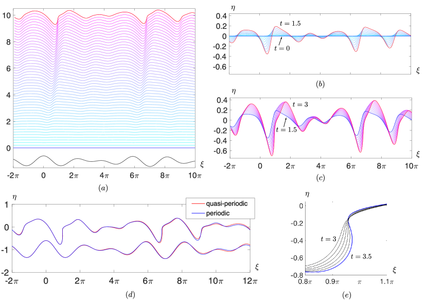
Figure 2. Panels (a)–(c) show the time evolution from $t=0$ to $t=3$ of an initially flat free surface in the presence of a background flow and a quasi-periodic bottom boundary. In panel (a), the bottom boundary is plotted in black and we added an upward spatial shift, given by (4.5), to separate the curves from each other. Panels (b) and (c) show details of the free surface without such a shift. In panel (d), we evolve this solution further, to $t=3.5$, and compare it to a periodic calculation with a bottom boundary of similar shape over the spatial range shown. Both waves overturn near $\xi=\pi$ and $t=3.3$. The evolution of the overturning periodic wave from $t=3$ to $t=3.5$ is shown in panel (e).

Figure 2 shows the time evolution of a free surface wave that is initially flat and develops quasi-periodic dynamics in the presence of a background flow and a quasi-periodic bottom boundary. In physical space, the bottom boundary is parameterized by

(4.4) $$\eta^{\text{b},\text{phys}}(x)=-1+0.2\cos(x)+0.2\cos(x/\sqrt{2})$$

and the mean velocity of the background flow in (2.28) is $\mathcal{U}=1$. In the computation, we use $M_{1}=M_{2}=512$ and compute the time evolution of the wave from $t=0$ to $t=3$ with time steps $\Delta t=10^{-5}$. In panel (a), the black line plots the bottom boundary and the blue line plots the flat free surface at $t=0$. To better distinguish the shape of the free surface at different times, we add an upward spatial shift to each curve. The time difference between two adjacent curves is 0.06, and we plot

(4.5) $$\eta^{\text{s}}(\alpha,t_{n})+10t_{n}/3,\qquad t_{n}=0.06n,\quad n=0,1,\ldots,50.$$

Due to the background flow and the quasi-periodic bottom boundary, the free surface wave moves from left to right and forms wave crests ahead of the peaks of the bottom boundary, which deflects the fluid upward. Panels (b) and (c) show snapshots of the time evolution of the free surface from $t=0$ to $t=1.5$ and from $t=1.5$ to $t=3$ separately without the upward shift given in (4.5); the time difference between two adjacent curves in both panels is 0.15.

In panel (d) of Figure 2, we further evolve the quasi-periodic wave from $t=3$ to $t=3.5$ using the same $512\times 512$ spatial grid on the torus and plot the free surface at $t=3.5$ with a red line. We find that the wave overturns near $\xi=\pi$ at $t=3.308$. However, the quasi-periodic wave is under-resolved by $t=3.5$, with gridpoints spread out enough to see discrete line segments in the plot near $\xi=\pi$ and small oscillations visible near $\xi=\pi$ and $\xi=7\pi$. In the infinite depth case [73], refining the grid to $4096\times 4096$ was sufficient to resolve an overturning spatially quasi-periodic wave so that the Fourier modes decay to $10^{-12}$ at all times. Here, rather than refine the mesh beyond $512\times 512$, we compute the time evolution of a periodic wave under the same initial condition and background flow, but with a periodic bottom boundary

(4.6) $$\eta^{\text{b},\text{phys}}(x)=-1+0.2\cos(x)+0.2\cos(5x/7),$$

where $5/7$ is a rational approximation of $k=1/\sqrt{2}$. We use the spatial resolution $M=32768$ for the periodic calculation (which employs 16385 Fourier modes). The free surface of the periodic wave at $t=3.5$ is plotted with a blue line in panel (d). We observe that the two waves in panel (d) resemble each other, but are not exactly the same, due to the different bottom boundaries. They will differ much more for larger values of $|x|$, where $\cos(x/\sqrt{2})$ is farther from $\cos(5x/7)$. The periodic wave overturns near $\xi=\pi$ at time $t=3.288$. We show the time evolution of the periodic wave near the overturning point from $t=3$ to $t=3.5$ in panel (e), where the time difference between adjacent curves is $\Delta t=0.1$.

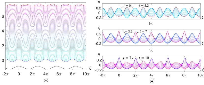
Figure 3. Time evolution from $t=0$ to $t=10$ of an initially periodic free surface evolving from rest, with no background flow, over a periodic bottom boundary whose spatial period is irrationally related to the initial period of the free surface. Panel (a) shows the free surface at different times with the upward shift (4.8); the bottom boundary is plotted in black. Panels (b), (c) and (d) show details of the free surface evolution without the shift.

Figure 3 shows the time evolution of an initially periodic free surface wave in the presence of a periodic bottom boundary whose spatial period is irrationally related to the initial condition. In physical space, the initial free surface and the bottom boundary are given by

(4.7) $$\eta^{\text{s},\text{phys}}_{0}(x)=0.2\cos(x),\qquad\qquad\eta^{\text{b},\text{phys}}(x)=-1+0.2\cos(x/\sqrt{2}).$$

In panel (a), the initial free surface and the bottom boundary are plotted with blue and black curves, respectively. As shown in the figure, they are both periodic and the bottom boundary’s wavelength is longer than that of the free surface. We use $M_{1}=M_{2}=256$ in the computation and evolve the water wave from $t=0$ to $t=10$ with time steps $\Delta t=2\times 10^{-5}$. At $t=0$, the fluid is at rest with zero velocity potential. In panel (a), we plot the time evolution of the free surface with an upward spatial shift

(4.8) $$\eta^{\text{s}}(\alpha,t_{n})+0.75t_{n},\qquad t_{n}=0.2n,\quad n=0,1,\ldots,50.$$

The free surface flattens due to the force of gravity and rises again due to inertia, which is similar to the oscillation of a standing water wave [42, 68]. One can observe that the crests and troughs of the surface wave are not symmetric for $t>0$ except at $x=0$ due to the even symmetry of the initial condition. In panels (b), (c) and (d), we plot snapshots of the time evolution of the free surface without the upward shift (4.8) from $t=0$ to $t=3.2$; from $t=3.2$ to $t=7$; and from $t=7$ to $t=10$. The time difference between two adjacent curves is 0.2. One can observe that the wave oscillates up and down like a standing wave. However, as a consequence of the quasi-periodic interactions between the surface wave and the bottom boundary, the heights of different crests are different at any given time.

4.2. Spatially quasi-periodic traveling waves

We formulate the traveling wave problem as a nonlinear least-squares problem, which we solve using a variant of the Levenberg-Marquardt algorithm [71, 48, 72]. In Section 3.1, we introduced the residual function $\mathcal{R}$ in (3.11), which depends on $\tau$, $b$, $\tilde{\eta}$, and demonstrated that the solutions of the traveling wave problem are the solutions of $\mathcal{R}[\tau,b,\tilde{\eta}]=0$. In the computation, we consider $\tau$, $b$ and the Fourier coefficients of $\tilde{\eta}$ as unknowns, denoted $\hat{\eta}$, and define the following scalar objective function

(4.9) $$\mathcal{F}[\tau,b,\hat{\eta}]:=\frac{1}{8\pi^{2}}\int_{\mathbb{T}^{2}}\mathcal{R}^{2}[\tau,b,\hat{\eta}]\,\,d\alpha_{1}\,d\alpha_{2}.$$

Note that solving (3.11) is equivalent to finding a zero of the objective function $\mathcal{F}[\tau,b,\hat{\eta}]$. For the unknown $\hat{\eta}$, we only vary the leading Fourier coefficients $\hat{\eta}_{j_{1},j_{2}}$ with $|j_{1}|\leq N_{1}<M_{1}/2$, $|j_{2}|\leq N_{2}<M_{2}/2$ and set the other Fourier coefficients to zero. According to the assumption (3.15), we also set $\hat{\eta}_{0,0}=0$ and require that the Fourier coefficients $\hat{\eta}_{j_{1},j_{2}}$ are real and satisfy $\hat{\eta}_{-j_{1},-j_{2}}=\hat{\eta}_{j_{1},j_{2}}$ . Consequently, the number of independent leading Fourier coefficients is $N_{\text{tot}}=N_{1}(2N_{2}+1)+N_{2}$. As discussed in Section 3.1, we choose $\hat{\eta}_{1,0}$, $\hat{\eta}_{0,1}$ and $h$ as bifurcation parameters when computing quasi-periodic traveling solutions bifurcating from the zero-amplitude solution and fix them at nonzero amplitudes in the minimization of $\mathcal{F}$. Therefore there are $N_{\text{tot}}$ parameters to compute, which are stored in a vector $\boldsymbol{p}$ as follows

(4.10) $$p_{1}=\tau,\quad p_{2}=\hat{\eta}_{1,1},\quad p_{3}=b,\quad p_{4}=\hat{\eta}_{1,-1},\quad p_{5}=\hat{\eta}_{0,2}\;\;,\;\;\dots\;\;,\;\;p_{N_{\text{tot}}}=\hat{\eta}_{1,-N_{2}}.$$

The Fourier modes have been organized in a spiral fashion so that low frequency modes appear first in the list and $\hat{\eta}_{1,0}$, $\hat{\eta}_{0,1}$ have been replaced by $\tau$ and $b$; see [72] for details. Our goal is to find $\boldsymbol{p}$ given $\hat{\eta}_{1,0}$ and $\hat{\eta}_{0,1}$ such that $\mathcal{F}[\boldsymbol{p};\hat{\eta}_{1,0},\hat{\eta}_{0,1}]=0$, where we have re-ordered the arguments of $\mathcal{F}$ and $\mathcal{R}$ in (4.9). In the computation, the function $\mathcal{R}$ is evaluated at $M_{1}\times M_{2}$ grid points, hence there are $M_{1}M_{2}$ equations, which are more than the number of unknowns. For this reason, the nonlinear least-squares problem is overdetermined.

The objective function $\mathcal{F}$ is computed from $\mathcal{R}$ by the trapezoidal rule approximation over $\mathbb{T}^{2}$, which is spectrally accurate,

(4.11) $$\begin{aligned} f(\boldsymbol{p})&=\frac{1}{2}r(\boldsymbol{p})^{T}r(\boldsymbol{p})\approx\mathcal{F}\left[\boldsymbol{p};\hat{\eta}_{1,0},\hat{\eta}_{0,1}\right],\\ r_{m}(\boldsymbol{p})&=\frac{\mathcal{R}\left[\boldsymbol{p};\hat{\eta}_{1,0},\hat{\eta}_{0,1}\right](\alpha_{m_{1}},\alpha_{m_{2}})}{\sqrt{M_{1}M_{2}}},\end{aligned}\quad\left(\begin{gathered}m=1+m_{1}+M_{1}m_{2}\\ \alpha_{m_{i}}=2\pi m_{i}/M_{i}\end{gathered}\right),\quad 0\leq m_{i}<M_{i}.$$

The parameters $p_{j}$ are chosen to minimize $f(\boldsymbol{p})$ using the Levenberg-Marquardt method [71, 48]. The method requires a Jacobian matrix $\partial r_{m}/\partial p_{j}$, which we compute by solving the variational equations (3.17). We have $\frac{\partial r_{m}}{\partial p_{j}}=\delta\mathcal{R}(\alpha_{m_{1}},\alpha_{m_{2}})/\sqrt{M_{1}M_{2}}$, where $m=1+m_{1}+M_{1}m_{2}$ and the $j$th column of the Jacobian corresponds to setting $\delta p_{j}$ in (4.10) to 1 and the others to 0 depending on the perturbation direction: $\delta\tau$, $\delta b$ or $\delta\hat{\eta}_{j_{1},j_{2}}$.

We compute quasi-periodic traveling solutions that bifurcate from the zero solution using $N_{x}=N_{y}=75$ and $M_{x}=M_{y}=200$. We fix $\hat{\eta}_{1,0}=\hat{\eta}_{0,1}=10^{-5}$, choose $h$ to be the continuation parameter, and decrease $h$ from 3 to 0.5 with $\Delta h=0.01$ to obtain a family of quasi-periodic solutions. In panel (a) of Figure 4, we plot the wave profile of the free surface for solutions at $h=0.5$ and $h=3$. The difference between these two solutions is small because they are both small-amplitude bifurcations from the zero solution for which we imposed the same amplitude parameters $\hat{\eta}_{1,0}$ and $\hat{\eta}_{0,1}$ at linear order. We stayed close to the linear regime in this example to investigate whether traveling solutions of the fully nonlinear equations, which we compute using the Levenberg-Marquardt method, behave as predicted by weakly nonlinear theory. While the wave profiles are close to one another, the values of $h$ (3 and 0.5) and $\tau$ (1.23088845108 and 0.0812490184995) differ substantially for the two solutions.

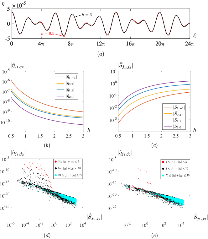
Figure 4. Quasi-periodic traveling gravity-capillary waves bifurcating from the zero solution. (a) Surface elevation function of two solutions with $h=0.5$ (dashed red line) and $h=3.0$ (solid black line). (b) Amplitudes of Fourier coefficients $\hat{\eta}_{2,0}$, $\hat{\eta}_{0,2}$, $\hat{\eta}_{1,1}$, $\hat{\eta}_{1,-1}$ of quasi-periodic traveling solutions for which $\hat{\eta}_{1,0}$ and $\hat{\eta}_{0,1}$ are fixed at $10^{-5}$. (c) Absolute value of the corresponding divisors $\hat{S}_{j_{1},j_{2}}$ defined by (3.27) in the weakly nonlinear model (3.31). Here we solve (3.11) by minimizing $f(\boldsymbol{p})$ in (4.11) and check whether the solution behaves as predicted by (3.31). Panels (d) and (e) show $|\hat{\eta}_{j_{1},j_{2}}|$ versus $|\hat{S}_{j_{1},j_{2}}|$ for $2\leq|j_{1}|+|j_{2}|\leq 75$ in the cases where $h=0.5$ and $h=3$, respectively.

In panel (b) of Figure 4, we plot the absolute value of the leading Fourier coefficients $|\hat{\eta}_{2,0}|$, $|\hat{\eta}_{0,2}|$, $|\hat{\eta}_{1,1}|$ and $|\hat{\eta}_{1,-1}|$ of the computed solutions as functions of $h$, holding $\hat{\eta}_{1,0}$ and $\hat{\eta}_{0,1}$ fixed at $10^{-5}$. These Fourier coefficients decrease as $h$ increases. In panel (c), we plot the absolute value of the divisors $\hat{S}_{j_{1},j_{2}}$ defined in (3.27) corresponding to these four Fourier coefficients, which decrease as $h$ decreases. The behavior of the Fourier coefficients and $\hat{S}_{j_{1},j_{2}}$ is consistent with the weakly nonlinear approximations (3.31), where the Fourier coefficients are obtained through division by $\hat{S}_{j_{1},j_{2}}$. As a result, smaller values of $\hat{S}_{j_{1},j_{2}}$ lead to larger Fourier coefficients. Note that we are checking whether traveling solutions of the Euler equations (3.11) obtained by minimizing $f(\boldsymbol{p})\approx\mathcal{F}\left[\boldsymbol{p};\hat{\eta}_{1,0},\hat{\eta}_{0,1}\right]$ in (4.11) via the Levenberg-Marquardt method behave as predicted by the weakly nonlinear model (3.31); we did not solve (3.31) directly.

Panels (d) and (e) of Figure 4 demonstrate the relationship between $|\hat{\eta}_{j_{1},j_{2}}|$ and $|\hat{S}_{j_{1},j_{2}}|$ with $2\leq|j_{1}|+|j_{2}|\leq 75$ for traveling solutions at $h=0.5$ and $h=3$, respectively. Since the largest Fourier coefficients are fixed at $10^{-5}$, one expects roundoff errors around $10^{-20}$. But instead the “roundoff floor,” visible in both panels, appears to grow linearly as $|\hat{S}_{j_{1},j_{2}}|$ decreases. This suggests that roundoff errors in the Levenberg-Marquardt method are amplified by the reciprocals of the divisors $\hat{S}_{j_{1},j_{2}}$ even though this is not a weakly nonlinear calculation. The “active” modes in which $\big{|}\hat{\eta}_{j_{1},j_{2}}\big{|}$ extends above the roundoff floor appear to be well-resolved. The plots look nearly identical if we refine the calculation, keeping $N_{x}=N_{y}=75$ but increasing $M_{x}$ and $M_{y}$ from 200 to 300. In fact, we plotted the data from this finer mesh in panels (d) and (e). In panel (e), when $h=3$, there are just a few active modes $\hat{\eta}_{j_{1},j_{2}}$, and they all correspond to low frequency modes with $2\leq|j_{1}|+|j_{2}|\leq 5$. But in panel (d), when $h=0.5$, there are many active modes of both small and intermediate frequency, plotted with red and black markers, respectively. This is consistent with (3.37) and panel (c), where the small divisors from weakly nonlinear theory decrease as $h$ decreases. The fixed values $\hat{\eta}_{1,0}=\hat{\eta}_{0,1}=10^{-5}$ we selected for this calculation appear to be small enough when $h=3$ that we could have computed the solution by weakly nonlinear theory, but large enough at $h=0.5$ that it was necessary to solve the problem by the Levenberg-Marquardt approach.

Next we search for quasi-periodic bifurcations from finite-amplitude periodic traveling waves of finite depth. We use a new procedure, described in detail for the case of deep water in [74], to locate bifurcation points. Specifically, we use the signed smallest singular value $\chi(s)$ of the Jacobian $\mathcal{J}^{\text{qua}}(s)$, as in (3.18), as a bifurcation “test function” that changes sign at bifurcation points. When a zero of $\chi(s)$ is found, the kernel of the Jacobian $\mathcal{J}^{\text{qua}}(s)$ of (3.18) also furnishes a search direction $\delta\tilde{\eta}^{\text{qua}}$ for the quasi-periodic branch. We use $\tilde{\eta}^{\text{per}}+\epsilon\delta\tilde{\eta}^{\text{qua}}$ with an empirically chosen value of $\epsilon$ as the initial guess for the Levenberg-Marquardt solver. We then use numerical continuation to follow this branch beyond the realm of linearization about the periodic traveling wave. Instead of using $\hat{\eta}_{1,0}$, $\hat{\eta}_{0,1}$ and $h$ as continuation parameters, we use $\tau$, $h$ and the Fourier mode $\hat{\eta}_{0,1}$. For simplicity, we hold $\tau$ and $h$ fixed and just vary the Fourier mode to obtain a one-parameter family of quasi-periodic solutions.

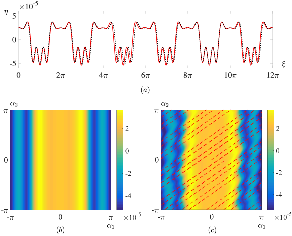
Figure 5. Quasi-periodic bifurcation from a periodic traveling gravity-capillary wave. Panel (a) shows the periodic traveling wave where a bifurcation was found and the largest-amplitude solution we computed on the quasi-periodic bifurcation branch. The dotted black line corresponds to the periodic wave and the red line corresponds to the quasi-periodic wave. Panels (b) and (c) show contour plots of the torus functions of the periodic wave and the quasi-periodic wave, respectively. The 1D quasi-periodic wave in panel (a) is extracted from the corresponding torus function along the characteristic lines of slope $k=1/\sqrt{2}$, plotted with red dashed lines in panel (c).

Figures 5 and 6 show two quasi-periodic gravity-capillary waves bifurcating from a branch of periodic traveling waves. The fluid depth in conformal space is $h=0.1$. We set $\tau=0.00327672209262$ so that the first Fourier mode of the periodic waves resonates with the fifth Fourier mode, which corresponds to solutions of the Wilton ripple problem [3, 62, 1]. For the periodic traveling wave, we set $M=300$, $N=100$ and use $s=\hat{\eta}_{1}$ as the continuation parameter. The 1D waves are computed on $\mathbb{T}$ and embedded in $\mathbb{T}^{2}$ when searching for bifurcations, so that $\hat{\eta}_{1}$ becomes $\hat{\eta}_{1,0}$. We computed periodic waves with amplitude $s$ ranging from $10^{-5}$ to $2\times 10^{-4}$ with $\Delta s=10^{-5}$. By tracking the sign of $\chi(s)$, we find out that there is a zero of $\chi(s)$ when $s$ belongs to intervals $[10^{-5},2\times 10^{-5}]$, $[4\times 10^{-5},5\times 10^{-5}]$, $[7\times 10^{-5},8\times 10^{-5}]$, $[1.1\times 10^{-4},1.2\times 10^{-4}]$ and $[1.7\times 10^{-4},1.8\times 10^{-4}]$. We focus our discussion on the first and last intervals and locate the zeros of $\chi(s)$ in these intervals, which are the bifurcation points, using the numerical algorithm described in [74]. In double precision, the zeros and corresponding values of $\chi$ are

(4.12) $$s_{1} =1.83810709940\times 10^{-5}, \quad\chi(s_{1}) =-7.8\times 10^{-15},$$

$$s_{2} =1.72625902886\times 10^{-4}, \quad\chi(s_{2}) =4.8\times 10^{-15}.$$

The periodic solutions at $s_{1}$ and $s_{2}$ are plotted with dotted black lines in panel (a) of Figures 5 and 6, respectively. These periodic solutions demonstrate the nonlinear interaction of Fourier modes of different wavelengths. Unlike the crests of sinusoidal waves, we observe small ripples at the wave peaks of the periodic wave at $s_{1}$. As the amplitude of the periodic solution increases, this nonlinear feature is more pronounced. For the periodic solution at $s_{2}$, near $x=2\pi n$ for $n\in\mathbb{Z}$, there is a flat plateau with wave peaks shifted to the edges of the plateau, forming an interesting “cat ears” structure. These nonlinear features at the wave crests can be attributed to the effect of the capillary force. In panel (b) of Figures 5 and 6, we show contour plots of torus functions of these periodic traveling waves. We observe that the width of the yellow region is larger for the higher-amplitude periodic wave; in correspondence, this wave possesses wider wave crests.

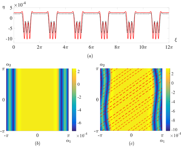
Figure 6. Quasi-periodic bifurcation from a larger-amplitude periodic traveling gravity-capillary wave. The panels show the same information as in Figure 5.

We compute secondary quasi-periodic bifurcation branches that intersect the primary periodic branch at $s_{1}$ and $s_{2}$ and show the corresponding results in Figures 5 and 6, respectively. In both computations, we set $M_{x}=300,M_{y}=150,N_{x}=100,N_{y}=50$ and use $\hat{\eta}_{0,1}$ as the continuation parameter. We follow the two quasi-periodic branches until $\hat{\eta}_{0,1}=7\times 10^{-5}$ and $\hat{\eta}_{0,1}=1.1\times 10^{-4}$, respectively; the corresponding quasi-periodic traveling waves are plotted with red lines in panel (a) of Figures 5 and 6. The objective function is minimized to $2.14\times 10^{-27}$ and $5.03\times 10^{-28}$, respectively, for these solutions. In panel (a) of Figure 5, the oscillations at the troughs of the quasi-periodic wave are ahead of the ones of the periodic wave near $\xi=3\pi,5\pi,7\pi,11\pi$ and are behind near $\xi=\pi$, which demonstrates the quasi-periodic feature of the secondary bifurcation.

We also observe that the amplitude of the quasi-periodic wave in panel (a) of Figure 5 is noticeably larger than the periodic wave due to the activation of Fourier modes in the quasi-periodic direction. In panel (c) of Figures 5 and 6, we show contour plots of the torus functions of the quasi-periodic traveling waves in panel (a). Unlike the periodic solution, the quasi-periodic solution depends on $\alpha_{2}$. For example, one can see the variation of the yellow and blue regions in the $\alpha_{2}$ direction. Moreover, this variation is rather oscillatory in Figure 5, which adds to the difficulty of computing higher-amplitude quasi-periodic waves on the bifurcation branch. The 1D quasi-periodic waves are obtained by evaluating the corresponding torus functions along the the red dashed line of slope $1/\sqrt{2}$. In panel (a) of Figures 5 and 6, there will be crests if the dashed line in panel (c) passes through the yellow region and troughs if it passes through the blue region. Due to the variation in yellow region, the widths of the crests of the quasi-periodic wave are no longer constant. For example, in panel (a) of Figure 6, the crests of the quasi-periodic wave are wider than those of the periodic wave near $\xi=6\pi,8\pi$ and narrower near $\xi=4\pi,10\pi$.

5. Conclusion

In this paper, we have presented a numerical study of two-dimensional finite-depth free surface waves in the spatially quasi-periodic setting. Specifically, we have studied both the initial value and traveling wave problems. For the initial value problem, we derived the governing equations of water waves in the presence of a background flow and a non-flat bottom boundary in conformal space. As noted in Remark 2.7, the derivation is valid in both the quasi-periodic and periodic settings. Motivated by the experiments of Torres et al. [61] studying spatially quasi-periodic surface waves in the presence of a quasi-periodic bottom boundary, we computed the time evolution of an initially flat surface with a background flow over a quasi-periodic bottom boundary. We also find that the waves develop quasi-periodic patterns in which the distance between adjacent wave peaks is not constant.

Next we computed spatially quasi-periodic traveling waves that bifurcate from the zero-amplitude wave or from finite-amplitude periodic traveling waves. Motivated by observations in [72, 74] that the Fourier coefficients of quasi-periodic traveling waves decay slower along certain directions, we derived the weakly nonlinear equations governing small-amplitude quasi-periodic traveling waves in Section 3.2 and found that there is a divisor $\hat{S}_{j_{1},j_{2}}$ in the formula for the Fourier coefficients $\hat{\eta}_{j_{1},j_{2}}$ of the weakly nonlinear solutions. For example, in the case of deep water, this divisor reads

(5.1) $$\hat{S}_{j_{1},j_{2}}=\frac{g}{k}(|j_{1}+kj_{2}|-k)(|j_{1}+kj_{2}|-1).$$

Due to the unboundedness of $1/\hat{S}_{j_{1},j_{2}}$, the Fourier coefficients along directions $|j_{1}+kj_{2}|-k=0$ and $|j_{1}+kj_{2}|-1=0$ are expected to decay slower than in other directions. We also study these divisors in the case of shallow water and find that weakly nonlinear theory breaks down faster when $h$ is smaller due to the factor of $h^{4}$ in the formula (3.37) for $\hat{S}_{j_{1},j_{2}}$.

In the current work, we assume that the bottom boundary remains fixed in time. In the future, we plan to further extend our method to study quasi-periodic flows with a free surface over a moving bottom boundary. In the case of periodic water waves, this has been studied in [56, 58]. We also plan to analyze the linear stability of periodic traveling waves [45, 18, 59, 50] and investigate the long-time dynamics of traveling waves under unstable subharmonic perturbations. In the quasi-periodic setting, we are able to compute the exact time evolution of these perturbed waves instead of their linearized approximations [36]. We are also interested in developing numerical methods, such as the Transformed Field Expansion method [46, 47, 52], to study the dynamics of these waves in three dimensions where the conformal mapping method no longer applies. On the theoretical side, a rigorous proof of the existence of quasi-periodic traveling waves is still an open problem. We expect it will be necessary to employ a Nash-Moser iteration to tackle the small divisor problem, which has been successfully used to prove the existence of temporally quasi-periodic standing waves and traveling waves [9, 8].

Funding: This work was supported in part by the National Science Foundation under award number DMS-1716560 and by the Department of Energy, Office of Science, Applied Scientific Computing Research, under award number DE-AC02-05CH11231; and by an NSERC (Canada) Discovery Grant.

Declaration of interests: The authors report no conflict of interest.

Appendix A Computation of the conformal mapping from a infinite horizontal strip to the fluid domain

In practice, the initial condition of the water wave is usually given in physical space. Therefore, we need to compute the conformal mapping $z(w,t)$ to transform the initial condition from physical space to conformal space. As shown in (2.22) and (2.23), the conformal mapping is determined by $h$, $x_{0}$, $\tilde{\eta}^{\text{s}}$ and $\tilde{\eta}^{\text{b}}$, where $x_{0}$ is fixed to be zero in the scope of this paper and $h$, $\tilde{\eta}^{\text{s}}$, $\tilde{\eta}^{\text{b}}$ are obtained by solving the following equations,

(A.1) $$\begin{gathered}\mathcal{R}_{1}(\alpha_{1},\alpha_{2})=\tilde{\eta}^{\text{s}}-\tilde{\eta}^{\text{s},\text{phys}}(\alpha_{1}+\tilde{\xi}^{\text{s}},\alpha_{2}+k\tilde{\xi}^{\text{s}})=0,\\ \mathcal{R}_{2}(\alpha_{1},\alpha_{2})=\tilde{\eta}^{\text{b}}-\tilde{\eta}^{\text{b},\text{phys}}(\alpha_{1}+\tilde{\xi}^{\text{b}},\alpha_{2}+k\tilde{\xi}^{\text{b}})=0,\\ \tilde{\xi}^{\text{s}}=H^{\coth}[\tilde{\eta}^{\text{s}}]+H^{\operatorname{csch}}[\tilde{\eta}^{\text{b}}],\qquad\qquad\tilde{\xi}^{\text{b}}=-H^{\operatorname{csch}}[\tilde{\eta}^{\text{s}}]-H^{\coth}[\tilde{\eta}^{\text{b}}],\end{gathered}$$

which come from (2.16) and (2.25). Moreover, we enforce the constraint $h=\hat{\eta}^{\text{s}}_{\boldsymbol{0}}-\hat{\eta}^{\text{b}}_{\boldsymbol{0}}$ discussed in Section 2.3 and rewrite $\tilde{\eta}^{\text{b}}$ as

(A.2) $$\tilde{\eta}^{\text{b}}=\hat{\eta}^{\text{s}}_{\boldsymbol{0}}-h+P[\tilde{\eta}^{\text{b}}].$$

Otherwise problem (A.1) is underdetermined and the solution is not unique.

In our computations, we consider $h$ and the Fourier coefficients of $\tilde{\eta}^{\text{s}}$ and $\tilde{\eta}^{\text{b}}$ as unknowns and define the following objective function

(A.3) $$\mathcal{F}[h,\hat{\eta}^{\text{s}},\hat{\eta}^{\text{b}}]: =\frac{1}{8\pi^{2}}\int_{\mathbb{T}^{2}}\mathcal{R}_{1}^{2}[h,\hat{\eta}^{\text{s}},\hat{\eta}^{\text{b}}]+\mathcal{R}_{2}^{2}[h,\hat{\eta}^{\text{s}},\hat{\eta}^{\text{b}}]\,\,d\alpha_{1}\,d\alpha_{2}$$

$$\approx\frac{1}{2M_{1}M_{2}}\sum_{m_{2}=0}^{M_{2}-1}\sum_{m_{1}=0}^{M_{1}-1}\Big{[}\mathcal{R}^{2}_{1}(2\pi m_{1}/M_{1},2\pi m_{2}/M_{2})+\mathcal{R}^{2}_{1}(2\pi m_{1}/M_{1},2\pi m_{2}/M_{2})\Big{]}.$$

We apply a Levenberg-Marquardt method [71] to solve the nonlinear least-squares problem (A.3) and compute the derivative of $\mathcal{R}_{1}$ and $\mathcal{R}_{2}$ with respect to the unknowns using the following variational equations

(A.4) $$\begin{gathered}\delta\mathcal{R}_{1}=\delta\tilde{\eta}^{\text{s}}-\tilde{\eta}^{\text{s},\text{phys}}_{x}\delta\tilde{\xi}^{\text{s}},\qquad\delta\mathcal{R}_{2}=\delta\hat{\eta}^{\text{s}}_{\boldsymbol{0}}-\delta h+P[\delta\tilde{\eta}^{\text{b}}]-\tilde{\eta}^{\text{b},\text{phys}}_{x}\delta\tilde{\xi}^{\text{b}},\\ \delta\tilde{\xi}^{\text{s}}=H^{\coth}[\delta\tilde{\eta}^{\text{s}}]+H^{\operatorname{csch}}[\delta\tilde{\eta}^{\text{b}}]+\big{(}\delta H^{\coth}\big{)}[\tilde{\eta}^{\text{s}}]+\big{(}\delta H^{\operatorname{csch}}\big{)}[\tilde{\eta}^{\text{b}}],\\ \delta\tilde{\xi}^{\text{b}}=-H^{\operatorname{csch}}[\delta\tilde{\eta}^{\text{s}}]-H^{\coth}[\delta\tilde{\eta}^{\text{b}}]-\big{(}\delta H^{\operatorname{csch}}\big{)}[\tilde{\eta}^{\text{s}}]-\big{(}\delta H^{\coth}\big{)}[\tilde{\eta}^{\text{b}}].\end{gathered}$$

Here $\partial_{x}=\partial_{x_{1}}+k\partial_{x_{2}}$ and the symbols of $\delta H^{\coth}$ and $\delta H^{\operatorname{csch}}$ are

(A.5) $$\delta\hat{H}^{\coth}_{j_{1},j_{2}}=\frac{i(j_{1}+kj_{2})\delta h}{\sinh^{2}((j_{1}+kj_{2})h)},\qquad\delta\hat{H}^{\operatorname{csch}}_{j_{1},j_{2}}=-i(j_{1}+kj_{2})\coth((j_{1}+kj_{2})h)\operatorname{csch}((j_{1}+kj_{2})h)\delta h.$$

References

• [1] B. Akers and D. P. Nicholls. Wilton ripples in weakly nonlinear dispersive models of water waves: Existence and analyticity of solution branches. Water Waves, 3:25–47, 2021.
• [2] B. F. Akers, D. M. Ambrose, and D. W. Sulon. Periodic travelling interfacial hydroelastic waves with or without mass ii: Multiple bifurcations and ripples. Europ. J. Appl. Math., 30(4):756–790, 2019.
• [3] B. F. Akers and W. Gao. Wilton ripples in weakly nonlinear model equations. Commun. Math. Sci., 10(3):1015–1024, 2012.
• [4] T. Alazard, N. Burq, and C. Zuily. On the Cauchy problem for gravity water waves. Invent. Math., 198(1):71–163, 2014.
• [5] D. M. Ambrose, R. Camassa, J. L. Marzuola, R. M. McLaughlin, Q. Robinson, and J. Wilkening. Numerical algorithms for water waves with background flow over obstacles and topography. Adv. Comput. Math., 48:46:1–62, 2022.
• [6] P. Baldi, M. Berti, E. Haus, and R. Montalto. Time quasi-periodic gravity water waves in finite depth. Invent. Math., 214(2):739–911, 2018.
• [7] M. Berti, L. Franzoi, and A. Maspero. Pure gravity traveling quasi-periodic water waves with constant vorticity. arXiv:2101.12006, 2021.
• [8] M. Berti, L. Franzoi, and A. Maspero. Traveling quasi-periodic water waves with constant vorticity. Arch. Rational Mech. Anal., 240:99–202, 2021.
• [9] M. Berti and R. Montalto. Quasi-periodic standing wave solutions of gravity-capillary water waves, volume 263 of Memoirs of the American Mathematical Society. American Mathematical Society, 2016.
• [10] I. V. Blinov. Periodic almost-schrödinger equation for quasicrystals. Scientific Reports, 5(1):1–5, 2015.
• [11] H. Bohr. Almost Periodic Functions. Dover, Mineola, New York, 2018.
• [12] R. P. Brent. Algorithms for minimization without derivatives. Prentice Hall, Inc., Englewood Cliffs, New Jersey, 1973.
• [13] T. Bridges and F. Dias. Spatially quasi-periodic capillary-gravity waves. Contemp. Math., 200:31–46, 1996.
• [14] B. Chen and P. Saffman. Numerical evidence for the existence of new types of gravity waves of permanent form on deep water. Stud. Appl. Math., 62(1):1–21, 1980.
• [15] W. Choi and R. Camassa. Exact evolution equations for surface waves. J. Eng. Mech., 125(7):756–760, 1999.
• [16] W. Craig and C. Sulem. Numerical simulation of gravity waves. J. Comput. Phys., 108:73–83, 1993.
• [17] D. Damanik and M. Goldstein. On the existence and uniqueness of global solutions for the kdv equation with quasi-periodic initial data. J. American Math. Soc., 29(3):825–856, 2016.
• [18] B. Deconinck and K. Oliveras. The instability of periodic surface gravity waves. J. Fluid Mech., 675:141, 2011.
• [19] B. Dodson, A. Soffer, and T. Spencer. The nonlinear Schrödinger equation on z and r with bounded initial data: Examples and conjectures. J. Stat. Phys., 180(1):910–934, 2020.
• [20] G. Ducrozet and M. Gouin. Influence of varying bathymetry in rogue wave occurrence within unidirectional and directional sea-states. J. Ocean Eng. and Mar. Energy, 3(4):309–324, 2017.
• [21] A. Dyachenko. On the dynamics of an ideal fluid with a free surface. Dokl. Math., 63(1):115–117, 2001.
• [22] A. I. Dyachenko, E. A. Kuznetsov, M. Spector, and V. E. Zakharov. Analytical description of the free surface dynamics of an ideal fluid (canonical formalism and conformal mapping). Phys. Letters A, 221(1-2):73–79, 1996.
• [23] A. I. Dyachenko, V. E. Zakharov, and E. A. Kuznetsov. Nonlinear dynamics of the free surface of an ideal fluid. Plasma Phys. Reports, 22(10):829–840, 1996.
• [24] S. Dyachenko. On the dynamics of a free surface of an ideal fluid in a bounded domain in the presence of surface tension. J. Fluid. Mech., 860:408–418, 2019.
• [25] I. A. Dynnikov and S. P. Novikov. Topology of quasi-periodic functions on the plane. Russ. Math. Surv., 60(1):1, 2005.
• [26] R. Feola and F. Giuliani. Quasi-periodic traveling waves on an infinitely deep perfect fluid under gravity, 2020. arXiv:2005.08280.
• [27] M. V. Flamarion, P. A. Milewski, and A. Nachbin. Rotational waves generated by current-topography interaction. Stud. Appl. Math., 142(4):433–464, 2019.
• [28] M. V. Flamarion, A. Nachbin, and R. Ribeiro. Time-dependent Kelvin cat-eye structure due to current–topography interaction. J. Fluid Mech., 889, 2020.
• [29] M. V. Flamarion and R. Ribeiro Jr. An iterative method to compute conformal mappings and their inverses in the context of water waves over topographies. Int. J. Numer. Methods Fluids, 93(11):3304–3311, 2021.
• [30] T. Gao, Z. Wang, and J.-M. Vanden-Broeck. On asymmetric generalized solitary gravity–capillary waves in finite depth. Proc. R. Soc. A, 472(2194):20160454, 2016.
• [31] E. Hairer, S. P. Norsett, and G. Wanner. Solving Ordinary Differential Equations I: Nonstiff Problems. Springer, Berlin, 2nd edition, 2000.
• [32] B. Harrop-Griffiths, M. Ifrim, and D. Tataru. Finite depth gravity water waves in holomorphic coordinates. Annals of PDE, 3(1):1–102, 2017.
• [33] J. G. Herterich and F. Dias. Extreme long waves over a varying bathymetry. J. Fluid Mech., 878:481–501, 2019.
• [34] J. K. Hunter, M. Ifrim, and D. Tataru. Two dimensional water waves in holomorphic coordinates. Commun. Math. Phys., 346(2):483–552, 2016.
• [35] G. Iooss, P. I. Plotnikov, and J. F. Toland. Standing waves on an infinitely deep perfect fluid under gravity. Arch. Rat. Mech. Anal., 177:367–478, 2005.
• [36] P. A. Janssen. Nonlinear four-wave interactions and freak waves. J. Phys. Ocean., 33(4):863–884, 2003.
• [37] R. S. Johnson. A modern introduction to the mathematical theory of water waves. Cambridge University Press, Cambridge, UK, 1997.
• [38] C. Kharif, J.-P. Giovanangeli, J. Touboul, L. Grare, and E. Pelinovsky. Influence of wind on extreme wave events: experimental and numerical approaches. J. Fluid Mech., 594:209–247, 2008.
• [39] C. Kittel. Introduction to Solid State Physics. John Wiley and Sons, New York, 8th edition, 2005.
• [40] Y. A. Li, J. M. Hyman, and W. Choi. A numerical study of the exact evolution equations for surface waves in water of finite depth. Stud. Appl. Math., 113(3):303–324, 2004.
• [41] D. I. Meiron, S. A. Orszag, and M. Israeli. Applications of numerical conformal mapping. J. Comput. Phys., 40(2):345–360, 1981.
• [42] G. N. Mercer and A. J. Roberts. Standing waves in deep water: Their stability and extreme form. Phys. Fluids A, 4(2):259–269, 1992.
• [43] P. A. Milewski, J.-M. Vanden-Broeck, and Z. Wang. Dynamics of steep two-dimensional gravity–capillary solitary waves. J. Fluid Mech., 664:466–477, 2010.
• [44] J. Moser. On the theory of quasiperiodic motions. SIAM Rev., 8(2):145–172, 1966.
• [45] D. P. Nicholls. Spectral stability of traveling water waves: Eigenvalue collision, singularities, and direct numerical simulation. Physica D, 240(4-5):376–381, 2011.
• [46] D. P. Nicholls and F. Reitich. A new approach to analyticity of Dirichlet-Neumann operators. Proc. R. Soc. Edinburgh A, 131(6):1411–1433, 2001.
• [47] D. P. Nicholls and F. Reitich. Stable, high-order computation of traveling water waves in three dimensions. Europ. J. Mech. B, 25(4):406–424, 2006.
• [48] J. Nocedal and S. J. Wright. Numerical Optimization. Springer, New York, 1999.
• [49] T. Oh. On nonlinear Schrödinger equations with almost periodic initial data. SIAM J. Math. Anal., 47(2):1253–1270, 2015.
• [50] R. Pierce and E. Knobloch. On the modulational stability of traveling and standing water waves. Phys. Fluids, 6(3):1177–1190, 1994.
• [51] P. Plotnikov and J. Toland. Nash-moser theory for standing water waves. Arch. Rat. Mech. Anal., 159:1–83, 2001.
• [52] S. Qadeer and J. Wilkening. Computing the Dirichlet–Neumann operator on a cylinder. SIAM J. Numer. Anal., 57(3):1183–1204, 2019.
• [53] R. Ribeiro, P. A. Milewski, and A. Nachbin. Flow structure beneath rotational water waves with stagnation points. J. Fluid Mech., 812:792–814, 2017.
• [54] V. Ruban. Water waves over a strongly undulating bottom. Phys. Rev. E, 70(6):066302, 2004.
• [55] V. Ruban. The Fermi-Pasta-Ulam recurrence and related phenomena for 1D shallow-water waves in a finite basin. J. Exper. Theoret. Phys., 114(2):343–353, 2012.
• [56] V. P. Ruban. Water waves over a time-dependent bottom: exact description for 2D potential flows. Phys. Letters A, 340:194–200, 2005.
• [57] V. P. Ruban. Numerical study of Fermi-Pasta-Ulam recurrence for water waves over finite depth. JETP Letters, 93(4):195–198, 2011.
• [58] V. P. Ruban. Waves over curved bottom: The method of composite conformal mapping. J. Exper. Theoret. Phys., 130(5):797–808, 2020.
• [59] R. Tiron and W. Choi. Linear stability of finite-amplitude capillary waves on water of infinite depth. J. Fluid Mech., 696:402, 2012.
• [60] A. Toffoli, M. Onorato, E. Bitner-Gregersen, A. R. Osborne, and A. V. Babanin. Surface gravity waves from direct numerical simulations of the euler equations: a comparison with second-order theory. Ocean Engineering, 35(3-4):367–379, 2008.
• [61] M. Torres, J. Adrados, J. Aragón, P. Cobo, and S. Tehuacanero. Quasiperiodic Bloch-like states in a surface-wave experiment. Phys. Rev. Letters, 90(11):114501, 2003.
• [62] O. Trichtchenko, B. Deconinck, and J. Wilkening. The instability of Wilton’s ripples. Wave Motion, 66:147–155, 2016.
• [63] K. Trulsen, H. Zeng, and O. Gramstad. Laboratory evidence of freak waves provoked by non-uniform bathymetry. Phys. Fluids, 24(9):097101, 2012.
• [64] J.-M. Vanden-Broeck. On periodic and solitary pure gravity waves in water of infinite depth. J. Eng. Math., 84(1):173–180, 2014.
• [65] C. Viotti and F. Dias. Extreme waves induced by strong depth transitions: Fully nonlinear results. Phys. Fluids, 26(5):051705, 2014.
• [66] C. Viotti, D. Dutykh, and F. Dias. The conformal-mapping method for surface gravity waves in the presence of variable bathymetry and mean current. Procedia IUTAM, 11:110–118, 2014.
• [67] Z. Wang, J.-M. Vanden-Broeck, and P. Milewski. Asymmetric gravity–capillary solitary waves on deep water. J. Fluid Mech., 759, 2014.
• [68] J. Wilkening. Breakdown of self-similarity at the crests of large amplitude standing water waves. Phys. Rev. Lett, 107:184501, 2011.
• [69] J. Wilkening. Relative-periodic elastic collisions of water waves. Contemp. Math., 635:109–129, 2015.
• [70] J. Wilkening. Traveling-standing water waves. Fluids, 6:187:1–35, 2021.
• [71] J. Wilkening and J. Yu. Overdetermined shooting methods for computing standing water waves with spectral accuracy. Comput. Sci. Discovery, 5(1):014017, 2012.
• [72] J. Wilkening and X. Zhao. Quasi-periodic travelling gravity-capillary waves. J. Fluid Mech., 915:A7:1–35, 2021.
• [73] J. Wilkening and X. Zhao. Spatially quasi-periodic water waves of infinite depth. J. Nonlinear Sci., 31:52:1–43, 2021.
• [74] J. Wilkening and X. Zhao. Spatially quasi-periodic bifurcations from periodic traveling water waves and a method for detecting bifurcations using signed singular values, 2022. arXiv:2208.05954.
• [75] J. Wilton. On ripples. Philos. Mag., 29(173):688–700, 1915.
• [76] V. E. Zakharov. Stability of periodic waves of finite amplitude on the surface of a deep fluid. J. Appl. Mech. Tech. Phys., 9(2):190–194, 1968.
• [77] V. E. Zakharov, A. I. Dyachenko, and O. A. Vasilyev. New method for numerical simulation of a nonstationary potential flow of incompressible fluid with a free surface. Eur. J. Mech. B Fluids, 21(3):283–291, 2002.
• [78] J. A. Zufiria. Symmetry breaking in periodic and solitary gravity-capillary waves on water of finite depth. J. Fluid Mech., 184:183–206, 1987.