Activity Detection for Grant-Free NOMA in Massive IoT Networks

Abstract

Recently, grant-free transmission paradigm has been introduced for massive Internet of Things (IoT) networks to save both time and bandwidth and transmit the message with low latency. In order to accurately decode the message of each device at the base station (BS), first, the active devices at each transmission frame must be identified. In this work, first we investigate the problem of activity detection as a threshold comparing problem. We show the convexity of the activity detection method through analyzing its probability of error which makes it possible to find the optimal threshold for minimizing the activity detection error. Consequently, to achieve an optimum solution, we propose a deep learning (DL)-based method called convolutional neural network (CNN)- activity detection (AD). In order to make it more practical, we consider unknown and time-varying activity rate for the IoT devices. Our simulations verify that our proposed CNN-AD method can achieve higher performance compared to the existing non-Bayesian greedy-based methods. This is while existing methods need to know the activity rate of IoT devices, while our method works for unknown and even time-varying activity rates.

I Introduction

Wireless technology recent advances provide massive connectivity for machines and objects resulting in the IoT [1]. The demand for the IoT is expected to grow drastically in the near future with numerous applications in health care systems, education, businesses and governmental services [2, 3, 4].

As the demand for connectivity in IoT systems is growing rapidly, it is crucial to improve the spectrum efficiency [5]. Hence, the non-orthogonal multiple access (NOMA) has been introduced [6]. To address the main challenges of IoT, including access collisions and massive connectivity, NOMA allows devices to access the channel non-orthogonally by either power-domain [7] or code-domain [8] multiplexing. Meanwhile, this massive connectivity is highly affected by the conventional grant-based NOMA transmission scheme, where the exchange of control signaling between the BS and IoT devices is needed for channel access. The excessive signaling overhead causes spectral deficiency and large transmission latency. Grant-free NOMA has been introduced to make a flexible transmission mechanism for the devices and save time and bandwidth by removing the need for the exchange of control signaling between the BS and devices. Hence, devices can transmit data randomly at any time slot without any request-grant procedure.

In many IoT applications, a few devices become active for a short period of time to communicate with the BS while others are inactive [9]. In IoT networks with a large number of nodes each with a small probability of activity, multiuser detection (MUD) methods heavily rely on AD prior to detection and decoding [4, 10, 11, 12, 13]. For uplink transmission in IoT systems with grant-free NOMA transmission scheme, where the performance of MUD can be severely affected by the multi-access interference, the reliable detection of both activity and transmitted signal is very challenging and can be computationally expensive [10, 12].

There have been many studies in the literature suggesting compressive sensing (CS) methods for joint activity and data detection [12, 13, 14, 15, 16]. Although CS methods can achieve a reliable MUD, they only work in networks with sporadic traffic pattern, and are expensive in terms of computational complexity [12]. Recently, DL models have observed a lot of interests in communication systems and more specifically in signal detection [17, 18, 19]. A study in [19] suggests to use DL for activity and data detection, however they consider a deterministic traffic pattern for the activity which is not valid in all environments.

In this work, we first formulate the problem of IoT activity detection as a threshold comparing problem. We then analyze the probability of error of this activity detection method. Observing that this probability of error is a convex function of the decision threshold, we raise the question of finding the optimal threshold for minimizing the activity detection error. To achieve this goal, we propose a CNN-based AD algorithm for grant-fee code-domain uplink NOMA. Unlike existing CS-based AD algorithms, our solution does not need to know the exact number of active devices or even the activity rate of IoT devices. In fact, in our system model we assume a time-varying and unknown activity rate and a heterogeneous network. Simulation results verify the success the proposed algorithm.

The rest of this paper is organized as follows. We present the system model in Section II. In Section III we formulate the device AD problem and derive its probability of error. Section IV introduces our CNN-based solution for device AD. The simulation results are presented in Section V. Finally, the paper is concluded in Section VI.

I-A Notations

Throughout this paper, $(\cdot)^{*}$ represents the complex conjugate. Matrix transpose and Hermitian operators are shown by $(\cdot)^{T}$ and $(\cdot)^{H}$, respectively. The operator $\text{diag}(\mathbf{b})$ returns a square diagonal matrix with the elements of vector $\mathbf{b}$ on the main diagonal. Furthermore, $\mathbb{E}[\cdot]$ is the statistical expectation, $\hat{\mathbf{a}}$ denotes an estimated value for $\mathbf{a}$, and size of set $\mathcal{S}$ is shown by $|\mathcal{S}|$. The constellation and $m$-dimensional complex spaces are denoted by $\mathbb{D}$ and $\mathbb{C}^{m}$, respectively. Finally, the circularly symmetric complex Gaussian distribution with mean vector $\mathbf{\mu}$ and covariance matrix $\mathbf{\Sigma}$ is denoted by $\mathcal{CN}(\mathbf{\mu},\mathbf{\Sigma})$.

II System Model

We consider a code-division multiple access (CDMA) uplink transmission, where $K$ IoT devices communicate with a single IoT BS equipped with $M$ receive antennas. This commonly used model [3, 6, 19], also considers a frame structure for uplink transmission composed of a channel estimation phase followed by CDMA slotted ALOHA data transmissions as shown in Fig. 1. In each frame, let $N_{\rm f}$ short packets of length $T_{\rm t}=N_{\rm s}T_{\rm s}$, where $N_{\rm s}$ is the number of symbols per IoT packet and $T_{\rm s}$ is the symbol duration. It is assumed that the channel is fixed during each frame, but it varies from one frame to another. The channel state information (CSI) is acquired at the BS during the channel estimation phase. As it is common in massive machine-type communications (mMTC), we assume that the IoT devices are only active on occasion and transmit short data packets during each frame. The activity rate of the IoT devices is denoted by $P_{\rm a}\in[0,P_{\rm max}]$, which is assumed to be unknown and time-varying from one packet transmission to another.

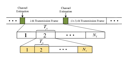
Figure 1: CDMA slotted ALOHA transmission frame

Let $b_{k}\in\cal A$ be the transmitted symbol of the $k$-th device and chosen from a finite alphabet $\cal A$, when the $k$-th device is active; otherwise, $b_{k}=0$. Consequently, $b_{k}$ can take values from an augmented alphabet $\bar{{\cal A}}={\cal A}\cup\{0\}$. We also denote the set of all devices and the set of active devices by ${\cal S}_{\rm t}=\{1,2,\dots,K\}$ and ${\cal S}_{\rm a}$, respectively, where ${\cal S}_{\rm a}\subset{\cal S}_{\rm t}$.

A unique spreading code is dedicated to each IoT device which is simultaneously used for the spreading purpose and device identification. This removes the need for control signaling associated with IoT device identification. Control signals are inefficient for short packet mMTC. The spreading sequence for the $k$-th IoT device is denoted by $\mathbf{c}_{k}=[c_{1,k}~{}~{}c_{2,k}~{}~{}\cdots~{}~{}c_{N_{c},k}]^{T}$ where $c_{i,k}\in\{-1,+1\}$ and $N_{\rm c}$ is the spreading factor. To support a large number of devices, non-orthogonal spreading sequences are employed; resulting in NOMA transmission.

For a single frame, the complex channel coefficient between the $k$-th IoT device and the $m$-th receive antenna at the BS is denoted as $g_{m,k}$. The active IoT device $k$, $k\in{\cal S}_{\rm a}$ transmits $N_{\rm s}$ symbols denoted by $\mathbf{b}_{k}=[b_{k,1},\cdots,b_{k,N_{\rm s}}]^{T}$ during a packet. The received baseband signal over Rayleigh flat fading channel in a single slot of the slotted ALOHA frame at the $m$-th receive antenna of the BS is expressed as

$$\mathbf{Y}_{m}=\sum_{k=1}^{K}g_{m,k}\mathbf{c}_{k}\mathbf{b}_{k}^{T}+\mathbf{W}_{m},$$ (1)

where $\mathbf{W}_{m}\in\mathbb{C}^{N_{\rm c}\times N_{\rm s}}$ with $w_{i,j}\sim{\cal CN}(0,\sigma_{\rm w}^{2})$ and $E[w_{i,j}w_{u,v}^{*}]=\sigma_{\rm w}^{2}\delta[i-u]\delta[j-v]$ is the additive white Gaussian noise (AWGN) matrix at the $m$-th receive antenna. The equivalent channel matrix between all IoT devices and the $m$-th receive antenna can be expressed as $\mathbf{\Phi}_{m}=[g_{m,1}\textbf{c}_{1},\cdots,g_{m,K}\textbf{c}_{K}]\in\mathbb{C}^{N_{\rm c}\times K}$. Thus, the received packet at the $m$-th ($m=1,2,\cdots,M$) receive antenna is given by

$$\mathbf{Y}_{m}=\mathbf{\Phi}_{m}\textbf{B}+\mathbf{W}_{m},$$ (2)

where $\textbf{B}=[\mathbf{b}_{1},\cdots,\mathbf{b}_{K}]^{T}\in\mathbb{D}^{K\times N_{\rm s}}$.

Let the total set of all IoT devices be decomposed into a finite number of disjoint groups $\mathcal{G}_{1},\mathcal{G}_{2},\cdots,\mathcal{G}_{S}$. Within group $\mathcal{G}_{j}$, the power of every IoT device is given by $P_{j}$. The powers of the devices are equal within each group, but differ from group to group. The fraction of devices in group $\mathcal{G}_{j}$ is therefore $|\mathcal{G}_{j}|/K$. It is assumed that $P_{j}$ is known at the BS. This configuration captures heterogeneous IoT networks, where groups of IoT devices capture different phenomenon in a given geographical area. A single group of IoT devices with equal power transmission, resulting in a homogeneous network, is also studied in this paper.

III Problem Formulation

In this section, we present the problem of IoT device AD in the cases of known CSI at the receiver and in the presence of sparse or non-sparse transmission. In order to detect the active devices, it is assumed that the BS is equipped with a match filter and the precoding matrix and CSI $\mathbf{\Phi}_{m}$ is available. Before AD, the observation matrix at the $m$-th receive antenna $\mathbf{y}_{m}$ is passed through the decorrelator to obtain

$$\mathbf{\overline{Y}}_{m}=\mathbf{\Phi}_{m}^{H}\mathbf{Y}_{m}\in\mathbb{C}^{K\times N_{\rm s}}.$$ (3)

In the following, we investigate the details of the AD problem based on the Gaussian detection to show how a threshold can be computed to distinguish active IoT devices from inactive ones. The output of the decorrelator receiver for the $m$-th receive antenna is expressed as

$$\mathbf{\overline{Y}}_{m}=\mathbf{\Phi}_{m}^{H}\mathbf{\Phi}_{m}\mathbf{B}+\mathbf{\Phi}_{m}^{H}\mathbf{W}_{m},$$

$$=\begin{bmatrix}\sum_{k=1}^{K}g_{m,1}^{*}g_{m,k}\mathbf{c}_{1}^{T}\mathbf{c}_{k}\mathbf{b}_{k}^{T}+g_{m,1}^{*}\mathbf{c}_{1}^{T}\mathbf{W}_{m}\\ \sum_{k=1}^{K}g_{m,2}^{*}g_{m,k}\mathbf{c}_{2}^{T}\mathbf{c}_{k}\mathbf{b}_{k}^{T}+g_{m,2}^{*}\mathbf{c}_{2}^{T}\mathbf{W}_{m}\\ \vdots\\ \sum_{k=1}^{K}g_{m,K}^{*}g_{m,k}\mathbf{c}_{K}^{T}\mathbf{c}_{k}\mathbf{b}_{k}^{T}+g_{m,K}^{*}\mathbf{c}_{K}^{T}\mathbf{W}_{m}\end{bmatrix}.$$ (4)

Consequently, the received signal from the $k$-th user at the $m$-th receive antenna is

$$\mathbf{r}_{k}^{m}=||g_{m,k}\mathbf{c}_{k}||_{2}^{2}\mathbf{b}_{k}^{T}+\sum_{i=1(i\neq k)}^{K}g_{m,k}^{*}g_{m,i}\mathbf{c}_{k}^{T}\mathbf{c}_{i}\mathbf{b}_{i}^{T}+g_{m,k}^{*}\mathbf{c}_{k}^{T}\mathbf{W}_{m},$$ (5)

where the second and third terms are multi user interference and additive noise, respectively. Since an IoT device is either active or inactive for the entire packet transmission, we determine the activity status of a device based on each received symbol and then use the results in [20] for spectrum sensing and combine the obtained results from all $N_{s}$ symbols. The device AD in the case of single symbol transmission is studied in [12], and we follow that to determine the status of each device based on each received symbol and then combine the results. The $j$-th received symbol from device $k$ at receive antenna $m$, denoted as $r_{k,j}^{m}$, is

$$r_{k,j}^{m}= ||g_{m,k}\mathbf{c}_{k}||_{2}^{2}b_{k,j}+$$

$$\sum_{i=1(i\neq k)}^{K}g_{m,k}^{*}g_{m,i}\mathbf{c}_{k}^{T}\mathbf{c}_{i}b_{i,j}+g_{m,k}^{*}\mathbf{c}_{k}^{T}\mathbf{w}_{j},$$ (6)

where the first term is the main signal, the second term is multi user interference from other devices, and the third term is the additive noise. For the sake of simplicity we assume that BPSK modulation is used, i.e., the transmitted symbols are drawn from ${\cal A}=\{-1,+1\}$ and $p(b_{k,j}=+1)=p(b_{k,j}=-1)=1/2$. The multi user interference plus noise in $r_{k,j}^{m}$ has variance

$$\sigma^{2}_{k,j}= \text{~{}var}\Big{\{}\sum_{i=1(i\neq k)}^{K}g_{m,k}^{*}g_{m,i}\mathbf{c}_{k}^{T}\mathbf{c}_{i}b_{i,j}+g_{m,k}^{*}\mathbf{c}_{k}^{T}\mathbf{w}_{j}\Big{\}}$$

$$= \sum_{i=1(i\neq k)}^{K}|g_{m,k}^{*}g_{m,i}\mathbf{c}_{k}^{T}\mathbf{c}_{i}|^{2}P_{a}+||g_{m,k}^{*}\mathbf{c}_{k}^{T}||_{2}^{2}.$$ (7)

Now we can approximate $r_{k,j}^{m}$ by a Gaussian distribution as ${\cal N}(||g_{m,k}\mathbf{c}_{k}||_{2}^{2},\sigma^{2}_{k,j})$ [20]. In order to identify the activity of device $k$, our goal is to propose an algorithm to define threshold $\tau$ and set device $k$ as active if $|r_{k,j}^{m}|>\tau$. Then the probability of error, $P_{e}$, is computed as

$$P_{e}^{k,j}= P_{a}p(|r_{k,j}^{m}|<\tau|b_{k,j}\neq 0)$$

$$+2(1-P_{a})p(|r_{k,j}^{m}|>\tau|b_{k,j}=0),$$ (8)

where we have $p(r_{k,j}^{m}|b_{k,j}\neq 0)\sim{\cal N}(||g_{m,k}\mathbf{c}_{k}||_{2}^{2},\sigma^{2}_{k,j})$ and $p(r_{k,j}^{m}|b_{k,j}=0)\sim{\cal N}(0,\sigma^{2}_{k,j})$. We can rewrite (III) as

$$P_{e}^{k,j}=2(1-P_{a})Q(\frac{\tau}{\sigma_{k,j}})+P_{a}Q(\frac{||g_{m,k}\mathbf{c}_{k}||_{2}^{2}-\tau}{\sigma_{k,j}}),$$ (9)

where $Q(x)=(1/\sqrt{2\pi})\int_{x}^{\infty}\exp(-t^{2}/2)dt$ denotes the Gaussian tail function. The probability of error in (9) is a convex function of $\tau$ and hence, a fine tuned neural network is capable of solving this problem and detect the active devices by finding the optimum $\tau$. In the following section, we define our DL-based algorithm to find the optimum $\tau$ and minimize the probability of error.

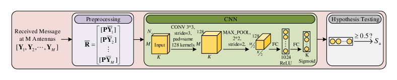
Figure 2: Model structure of the proposed CNN-AD algorithm

IV DL-Based AD

Device AD is the first step toward effective MUD in a grant-free uplink multiple access. The recent studies on AD suggest to use CS methods to identify the set of active devices [14, 15]. However, these methods fail in the practical scenarios, where the activity rate is time-varying and/or unknown. Moreover, these methods are mainly effective for low device activity rate scenarios, i.e., when sparsity level is high [14]. In this section, we propose our AD algorithms called CNN-AD by employing a CNN for heterogeneous IoT networks. By employing a suitably designed CNN, the underlying pattern in device activity can be easily learnt.

IV-A CNN-AD Algorithm

Fig. 2 illustrates the structure of the proposed CNN-AD algorithm. As seen, it is composed of there blocks: 1) preprocessing, 2) CNN processing, and 3) hypothesis testing.

In the preprocessing step after sequence matched filtering, we first sort the observation matrix from all $M$ receive antennas in a 3D Tensor as

$${\mathbf{\overline{R}}}=\left[\begin{array}[]{l}\left[{{\bf{P}}{{{\bf{\bar{Y}}}}_{1}}}\right]\\ \left[{{\bf{P}}{{{\bf{\bar{Y}}}}_{2}}}\right]\\ \,\,\,\,\,\vdots\\ \left[{{\bf{P}}{{{\bf{\bar{Y}}}}_{M}}}\right]\end{array}\right]$$ (14)

where $\mathbf{P\overline{Y}}_{m}\in\mathbb{C}^{K\times N_{\rm s}}$, $\mathbf{\overline{Y}}_{m}=\mathbf{\Phi}_{m}^{H}\mathbf{Y}_{m}\in\mathbb{C}^{K\times N_{\rm s}}$ for $m=1,2,\cdots,M$, and $\textbf{P}\triangleq{\rm diag}(p_{1},\cdots,p_{K})$, $p_{k}\in\{1/P_{1},\cdots,1/P_{S}\}$ for $k=1,2,\cdots,K$.

In the CNN processing block, the 3D Tensor $\mathbf{\overline{R}}$ is used as the input of a suitable designed CNN. The CNN models benefit from the convolutional layers performing convolution operations between matrices instead of multiplication. Thus, it leads to dimension reduction for feature extraction and provides a new input to the next network layers which includes only the useful features of the original high-dimensional input. The IoT device AD can be formulated as a binary classification or regression problem. Formulating device AD as a classification problem is straightforward, but it requires the accurate design of the CNN’s structure and parameters.

In the hypothesis testing block, the $K$ outputs of the CNN’s Sigmoid layer is compared with a predefined threshold to determine the activity status of the IoT devices in the network. If the $k$-th node of the Sigmoid layer exceeds the threshold, the $k$-th IoT device is identified as active.

IV-B Training Phase

In order to train the designed CNN, we define the activity vector $\mathbf{a}$ as

$$\mathbf{a}=[a_{1}~{}~{}a_{2}~{}~{}\cdots~{}~{}a_{K}]^{T},$$ (15)

where $a_{k}$ is 1 when the $k$-th IoT device is active and 0 otherwise. We train our model with $N$ independent training samples ($\mathbf{\overline{R}}^{(j)}$,$\mathbf{a}^{(j)}$), where $j=1,2,\cdots,N$ and $\mathbf{a}^{(j)}$ and $\mathbf{\overline{R}}^{(j)}$ are the activity vector and observation matrix of the $j$-th training sample, respectively. Our objective is to train the designed CNN to generate the desired output vector $\mathbf{a}^{(j)}$ for input matrix $\mathbf{\overline{R}}^{(j)}$. The model tries to learns non-linear transformation $\Psi$ such that

$$\mathbf{\hat{a}}^{(j)}=\Psi(\mathbf{\overline{R}}^{(j)};\bf{\Theta}),$$ (16)

where $\bf{\Theta}$ is the set of parameters learned during the training by minimizing the loss function. The output of model, i.e. $\mathbf{\hat{a}}$ determines the activity probabilities of the IoT devices. Here since there are two classes (active or inactive) for each IoT device, the loss function is chosen as the binary cross-entropy. For each training sample $j$, the binary cross-entropy loss function compares the probability that the IoT devices are active ($\mathbf{\hat{a}}^{(j)}$) with the true activity vector $\mathbf{a}^{(j)}$ as

$$\text{Loss}{(\bf{\Theta})}=\frac{1}{N}\sum_{j=1}^{N}-\Big{(}\mathbf{a}^{(j)}\log(\mathbf{\hat{a}}^{(j)})+({\bf{1}}-\mathbf{a}^{(j)})\log({\bf 1}-\mathbf{\hat{a}}^{(j)})\Big{)},$$ (17)

where $\log(\cdot)$ performs an element-wise $\log$ operation on $\mathbf{\hat{a}}^{(j)}$, and the vector multiplication is also element-wise.

V Experiments

In this section, we evaluate the performance of the proposed CNN-AD algorithm through various simulation experiments and compare it with some of the existing methods.

V-A Simulation Setup

We consider an IoT network with $K$ devices where $K>N_{\rm c}$ and pseudo-random codes are used as the spreading sequences for IoT devices. The probability of activity $P_{\rm a}$ is considered to be unknown and time-varying from one packet to another in the range of $P_{\rm a}\in[0,P_{\rm max}]$, where $P_{\rm max}=0.1$. The BPSK modulation is used for uplink transmission. Without loss of generality, the channel coefficient between IoT devices and the BS is modeled as independent zero-mean complex Gaussian random variables with variance $\sigma_{k,m}^{2}=1,k\in{\cal S}_{\rm t}$ and $m\in\{1,\cdots,M\}$. The additive white noise is modeled as zero-mean complex Gaussian random variables with variance $\sigma_{\rm w}^{2}$, and the signal-to-noise ratio (SNR) in dB is defined as $\gamma\triangleq 10\log(\sigma_{\rm{s}}^{2}/\sigma_{\rm{w}}^{2})$, where $\sigma_{\rm{s}}^{2}=P_{\rm a}P_{\rm t}$ is the average transmit power with $P_{\rm t}=\sum_{k=1}^{K}p_{k}$ as the total transmission power. Unless otherwise mentioned, we consider spreading sequences with spreading factor $N_{\rm c}=32$.

In order to train CNN-AD, we generate $10^{5}$ independent samples and use 80% for training and the rest for validation and test. Adam optimizer [21] with learning rate of $10^{-3}$ is used to minimize cross-entropy loss function in (17).

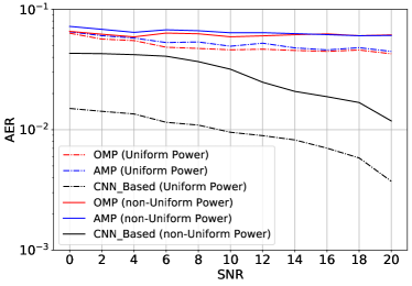
Figure 3: Achieved BER with MMSE with a priory AD of OMP, AMP, and CNN-AD without knowing the number of active devices.

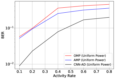
Figure 4: Impact of $P_{\rm a}$ on the performance of different methods as the priory AD for MMSE in terms of achieved BER.

V-B Simulation Results

V-B1 Performance Evaluation of CNN-AD

We assess CNN-AD through various simulations and compare it with the existing CS-based methods including orthogonal matching pursuit (OMP) [22] and approximate message passing (AMP) [23].

The impact of SNR on the activity error rate (AER) achieved by different AD algorithms in both homogeneous and heterogeneous IoT networks with uniform and non-uniform power allocation is shown in Fig. 3. The AER of different methods are compared for a wide range of SNRs in an IoT system with total $K=40$ IoT devices and a single BS with $M=100$ receive antennas. As expected, the AER of all AD algorithms decreases with increasing SNR. However, CNN-AD achieves the best performance since unlike the non-Bayesian greedy algorithms OMP and AMP, our method relies on the statistical distributions of device activities and channels and exploit them in the training process.

Fig. 4 illustrates the effect of activity rate on the bit error rate (BER) for minimum mean square error (MMSE)-MUD with different AD algorithms at $\gamma=10$ dB SNR. As seen, as the activity rate increases, the number of active devices also increases accordingly and thus it becomes difficult to detect all the active devices. This results in a higher BER. We use $P_{\rm max}=0.1$ to train CNN-AD. Thus, the MMSE-MUD with CNN-AD shows performance degradation for the activity rates of larger than $P_{\rm max}=0.1$. However, it still outperforms the performance of the MMSE-MUD with OMP and AMP AD algorithms. It should be mentioned that this performance improves when CNN-AD is trained for a larger value of $P_{\rm max}$.

We further investigate the AD algorithms in terms of other metrics for two typical IoT devices for $P_{\rm max}=0.1$ at $\gamma=10$ dB SNR, presented in Table I. In this table we compare the precision, recall, and F1-score, defined in [24], achieved by CNN-AD with OMP and AMP AD algorithms. As seen, all metrics are improved by using CNN-AD.

IoT Device	Model	Precision	Recall	F1-score
	OMP	28%	32%	30%
Device A	AMP	31%	35%	33%
	CNN-AD	73%	92%	81%
	OMP	33%	32%	32%
Device B	AMP	38%	35%	36%
	CNN-AD	100%	83%	91%

TABLE I: Performance analysis different algorithms for two typical IoT devices for $P_{\rm max}=0.1$ at $\gamma=10$ dB.

VI Conclusions

In this paper, we consider the problem of AD in IoT networks in grant-free NOMA systems. Based on the application, IoT devices can be inactive for a long period of time and only active in the time of transmission to the BS. Hence, identifying the active devices is required for an accurate data detection. Some studies propose CS-based method for AD. However, high level of message sparsity is necessary for those methods. In order to remove this need and exploit the statistical properties of the channels we propose a CNN-based method called CNN-AD to detect active IoT devices. Comparison with available methods shows the strength of our algorithm.

References

- [1] G. Durisi, T. Koch, and P. Popovski, “Toward massive, ultrareliable, and low-latency wireless communication with short packets,” Proceedings of the IEEE, vol. 104, no. 9, pp. 1711–1726, 2016.
- [2] L. D. Xu, W. He, and S. Li, “Internet of things in industries: A survey,” IEEE Transactions on Industrial Informatics, vol. 10, no. 4, pp. 2233–2243, 2014.
- [3] A. Al-Fuqaha, M. Guizani, M. Mohammadi, M. Aledhari, and M. Ayyash, “Internet of Things: A survey on enabling technologies, protocols, and applications,” IEEE Communications Surveys Tutorials, vol. 17, no. 4, pp. 2347–2376, 2015.
- [4] C. Bockelmann, N. Pratas, H. Nikopour, K. Au, T. Svensson, C. Stefanovic, P. Popovski, and A. Dekorsy, “Massive machine-type communications in 5G: Physical and MAC-layer solutions,” IEEE Communications Magazine, vol. 54, no. 9, pp. 59–65, 2016.
- [5] W. Ejaz and M. Ibnkahla, “Multiband spectrum sensing and resource allocation for IoT in cognitive 5G networks,” IEEE Internet of Things Journal, vol. 5, no. 1, pp. 150–163, 2018.
- [6] Z. Ding, P. Fan, and H. V. Poor, “Impact of user pairing on 5G nonorthogonal multiple-access downlink transmissions,” IEEE Transactions on Vehicular Technology, vol. 65, no. 8, pp. 6010–6023, 2016.
- [7] Y. Saito, Y. Kishiyama, A. Benjebbour, T. Nakamura, A. Li, and K. Higuchi, “Non-orthogonal multiple access (NOMA) for cellular future radio access,” in 2013 IEEE 77th Vehicular Technology Conference (VTC Spring), 2013, pp. 1–5.
- [8] K. Au, L. Zhang, H. Nikopour, E. Yi, A. Bayesteh, U. Vilaipornsawai, J. Ma, and P. Zhu, “Uplink contention based SCMA for 5G radio access,” in 2014 IEEE Globecom Workshops (GC Wkshps), 2014, pp. 900–905.
- [9] L. Liu, E. G. Larsson, W. Yu, P. Popovski, C. Stefanovic, and E. de Carvalho, “Sparse signal processing for grant-free massive connectivity: A future paradigm for random access protocols in the Internet of Things,” IEEE Signal Processing Magazine, vol. 35, no. 5, pp. 88–99, Sep. 2018.
- [10] S. Verdu et al., Multiuser detection. Cambridge university press, 1998.
- [11] Y. Zhang, Q. Guo, Z. Wang, J. Xi, and N. Wu, “Block sparse bayesian learning based joint user activity detection and channel estimation for grant-free noma systems,” IEEE Transactions on Vehicular Technology, vol. 67, no. 10, pp. 9631–9640, 2018.
- [12] H. Zhu and G. B. Giannakis, “Exploiting sparse user activity in multiuser detection,” IEEE Transactions on Communications, vol. 59, no. 2, pp. 454–465, Feb. 2011.
- [13] H. F. Schepker, C. Bockelmann, and A. Dekorsy, “Coping with CDMA asynchronicity in compressive sensing multi-user detection,” in 2013 IEEE 77th Vehicular Technology Conference (VTC Spring), Jun. 2013, pp. 1–5.
- [14] Z. Chen, F. Sohrabi, and W. Yu, “Sparse activity detection for massive connectivity,” IEEE Transactions on Signal Processing, vol. 66, no. 7, pp. 1890–1904, Apr. 2018.
- [15] K. Takeuchi, T. Tanaka, and T. Kawabata, “Performance improvement of iterative multiuser detection for large sparsely spread CDMA systems by spatial coupling,” IEEE Transactions on Information Theory, vol. 61, no. 4, pp. 1768–1794, Apr. 2015.
- [16] Y. Wang, X. Zhu, E. G. Lim, Z. Wei, Y. Liu, and Y. Jiang, “Compressive sensing based user activity detection and channel estimation in uplink noma systems,” in 2020 IEEE Wireless Communications and Networking Conference (WCNC). IEEE, 2020, pp. 1–6.
- [17] I. Goodfellow, Y. Bengio, and A. Courville, Deep learning. MIT press Cambridge, 2016, vol. 1.
- [18] M. Mohammadkarimi, M. Mehrabi, M. Ardakani, and Y. Jing, “Deep learning based sphere decoding,” IEEE Trans. Wireless Commun., pp. 1–1, 2019.
- [19] X. Miao, D. Guo, and X. Li, “Grant-free NOMA with device activity learning using long short-term memory,” IEEE Wireless Communications Letters, pp. 1–1, 2020.
- [20] W. Zhang, R. K. Mallik, and K. B. Letaief, “Cooperative spectrum sensing optimization in cognitive radio networks,” in 2008 IEEE International Conference on Communications, 2008, pp. 3411–3415.
- [21] D. P. Kingma and J. Ba, “Adam: A method for stochastic optimization,” arXiv preprint arXiv:1412.6980, 2014.
- [22] T. T. Cai and L. Wang, “Orthogonal matching pursuit for sparse signal recovery with noise,” IEEE Transactions on Information theory, vol. 57, no. 7, pp. 4680–4688, 2011.
- [23] D. L. Donoho, A. Maleki, and A. Montanari, “Message-passing algorithms for compressed sensing,” Proceedings of the National Academy of Sciences, vol. 106, no. 45, pp. 18 914–18 919, 2009.
- [24] C. Goutte and E. Gaussier, “A probabilistic interpretation of precision, recall and f-score, with implication for evaluation,” in European conference on information retrieval. Springer, 2005, pp. 345–359.