Supplementary material

In this supplementary material, we derive the relationship between superfluidity and elementary excitation properties. We also derive a hydrodynamics model to analyze the angle rotation of Bose-Einstein condensates in harmonic trap in the small period lattice case.

I Superfluid sum-rule and sound velocity

The superfluid density is explicitly related to Green function of the many-body Hamiltonian via the Josephson sum-rule [clark2013mathematical]. Here we derive the sum-rule and relate it to the measurable quantities of the anisotropic sound velocities.

We consider the variation of the condensate wavefunction $\psi(x)=\sqrt{|\psi|}\exp[i\phi({\bf r})]$ from a perturbation Hamiltonian $H^{\prime}=-\int d\bf r\psi(\bf r)\xi(\bf r)$, where $\xi(\bf r)=\xi\exp{i(k\cdot r-\omega t)}$. According to linear response theory

$$\delta\langle\psi(\mathbf{r})\rangle=e^{ik\cdot r-i\omega t}\xi\int_{-\infty}^{\infty}d\omega^{\prime}\frac{\mathbf{A}(\mathbf{k},\omega^{\prime})}{\omega+i\eta-\omega^{\prime}},$$ (1)

where $A(\bm{k},\omega)=\int d\mathbf{r}e^{-i\bm{k}\cdot\left(\bm{r}-\bm{r}^{\prime}\right)}\int_{-\infty}^{\infty}dte^{i\omega\left(t-t^{\prime}\right)}\left\langle\left[\psi(\bm{r},t),\psi^{\dagger}\left(\bm{r}^{\prime},t^{\prime}\right)\right]\right\rangle$ is the spectral density, and is related to the retarded one-body Green function

$$A(\mathbf{k},\omega)=i\hbar\int d\left(\mathbf{r}-\mathbf{r}^{\prime}\right)e^{-i\mathbf{k}\left(\mathbf{r}-\mathbf{r}^{\prime}\right)}\int_{-\infty}^{\infty}d\left(t-t^{\prime}\right)e^{i\omega\left(t-t^{\prime}\right)}G^{\mathrm{ret}}\left(\mathbf{r},t;\mathbf{r}^{\prime},t^{\prime}\right).$$

Similarly, the variation of the current operator $\bf J(r)=\rho v$ is

$$\delta\langle\mathbf{J}(r)\rangle=e^{i\mathbf{k}\cdot\mathbf{r}-i\omega t}\xi\int d\omega^{\prime}\frac{\mathbf{\Gamma}\left(\mathbf{k},\omega^{\prime}\right)}{\omega+i\eta-\omega^{\prime}}$$ (2)

with $\Gamma(k,\omega)=\int d\mathbf{r}dte^{-i\omega\left(t-t^{\prime}\right)+ik\left(r-r^{\prime}\right)}\langle\left[J(r,t),\psi^{\dagger}\left(r^{\prime},t^{\prime}\right)\right]\rangle.$ In the next we first take $\omega\rightarrow 0$ limit, and then take $\mathbf{k}\rightarrow 0$.

We want to relate $\bf\delta\langle J(r)\rangle$ to $\delta\langle\psi(\bf r)\rangle$, as to define the superfluid density. To do that, one observes from the continuity equation $-i\mathbf{k}\cdot\mathbf{J}=\partial_{t}\rho$ so that

$$\mathbf{J}(\mathbf{r},t)=\int d\mathbf{k}\mathbf{J}(\mathbf{k},t)e^{ik\cdot r}=\int d\mathbf{k}d\mathbf{r}^{\prime}e^{ik\left(r-r^{\prime}\right)}\frac{i\vec{k}}{k^{2}}\partial_{t}\rho(r^{\prime},t).$$

Plug it back to equation 2, and after some algebra

$$\Gamma(\mathbf{k},\omega) =\int d\mathbf{r}dte^{-i\omega\left(t-t^{\prime}\right)+ik\left(r-r^{\prime}\right)}\int d\mathbf{k}^{\prime}d\mathbf{r}^{\prime\prime}e^{ik^{\prime}\left(r-r^{\prime\prime}\right)}\frac{i\vec{k^{\prime}}(-i\omega)}{k^{\prime 2}}\langle\left[\rho\left(r^{\prime\prime},t\right),\psi^{\dagger}\left(r^{\prime},t^{\prime}\right)\right]\rangle$$ (3)

$$=\int dte^{-i\omega\left(t-t^{\prime}\right)}\int d\mathbf{r}^{\prime\prime}e^{ik\left(r^{\prime\prime}-r^{\prime}\right)}\frac{\mathbf{k}\omega}{k^{2}}\langle\left[\rho\left(r^{\prime\prime}t\right),\psi^{\dagger}\left(r^{\prime}t^{\prime}\right)\right]\rangle$$

Hence

$$\delta\langle\mathbf{J}(\mathbf{r},t)\rangle =\int d\omega^{\prime}\frac{\mathbf{\Gamma}\left(k,\omega^{\prime}\right)}{-\omega^{\prime}}e^{i\mathbf{k}r}\xi$$ (4)

$$=-\int d\omega e^{i\mathbf{k}r}\xi\int dte^{-i\omega\left(t-t^{\prime}\right)}\int d\mathbf{r}e^{ik\cdot(r-r^{\prime})}\frac{\vec{k}}{k^{2}}\langle\left[\rho(r,t),\psi^{\dagger}\left(r^{\prime},t^{\prime}\right)\right]\rangle$$

$$=-e^{i\mathbf{k}r}\xi\int d\mathbf{r}e^{i\mathbf{k}\cdot\left(r-r^{\prime}\right)}\frac{\vec{k}}{k^{2}}\left\langle\left[\rho(rt),\psi^{\dagger}\left(r^{\prime}t\right)\right]\right\rangle$$

$$=-e^{ik\cdot r}\xi\frac{k}{k^{2}}\left\langle\psi^{\dagger}(r,t)\right\rangle$$

In the last equality we used $\left[\rho(r),\psi^{\dagger}\left(r^{\prime}\right)\right]=\left[\psi^{\dagger}(r)\psi(r),\psi^{\dagger}\left(r^{\prime}\right)\right]=\psi^{\dagger}(r)\delta\left(r-r^{\prime}\right)$.

For a superfluid system, $\langle\psi(\mathbf{r})\rangle=\psi_{0}+\delta\langle\psi(\mathbf{r})\rangle=e^{i\theta(\mathbf{r})}\psi_{0}$ where we have defined the superfluid phase $\theta(\mathbf{r})$. With the periodic modulation of density introduced by the optical lattice, we take $\psi(\mathbf{r})\rightarrow\bar{\psi}(\mathbf{r})=a_{x}a_{y}a_{z}\int_{\mathrm{UC}}d\mathbf{r}\psi(\mathbf{r})$.[muller2015josephson] Now we have

$$\delta\langle\bar{\mathbf{J}}\rangle=-e^{i\mathbf{k}\cdot r}\xi\frac{\mathbf{k}}{k^{2}}\left\langle\bar{\psi}^{\dagger}\right\rangle$$

$$\delta\langle\bar{\psi}\rangle=-e^{i\mathbf{k}\cdot r}\xi\int d\omega\frac{A(k,\omega)}{\omega}$$

$$\frac{m}{\hbar}\delta\langle\bar{\mathbf{J}}\rangle=\rho^{sf}\nabla\theta=\rho^{sf}\nabla\frac{\delta\langle\bar{\psi}\rangle}{i\bar{\psi}_{0}}=\rho_{\hat{k}}^{sf}\mathbf{k}\frac{\delta\langle\bar{\psi}\rangle}{\bar{\psi}_{0}}$$

and take $\mathbf{k}\rightarrow 0$

$$\rho_{\hat{k}}^{sf}=m\lim_{\mathbf{k}\rightarrow 0}\frac{\bar{\psi}_{0}^{*}\bar{\psi}_{0}}{k^{2}\int_{-\infty}^{+\infty}d\omega\frac{\mathbf{A}(k,\omega)}{\omega}}$$ (5)

where $\rho_{\hat{k}}^{sf}=\rho_{ij}^{sf}\mathbf{\hat{k}}_{j}$. For homogeneous weakly interacting Bose gas at $T=0$, the Bogoliubov theory gives $\mathbf{A}(\mathbf{k},\omega)=\frac{mc}{2k}[\delta(\omega-ck)-\delta(\omega+ck)]$ as $k\rightarrow 0$, which leads to $\rho_{\hat{k}}^{sf}=|\psi_{0}|^{2}$. For anisotropic systems, the poles of $\mathbf{A}(\mathbf{k},\omega)$ i.e. the sound velocities along different directions will determine the anisotropic superfluid density.

The modification of the phonon spectrum by the presence of a shallow optical lattice is numerically computed through Bogoliubov-de-Gennes equations applied upon the mean-field ground state found by a 2D GPE imaginary time simulation. The lattice changes the sound velocity ratio while opening a gap at the Brillouin zone edge, as in Fig. S1.

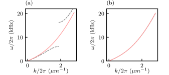
Figure S1: Modification of the phonon spectrum by the $a=266$ nm optical lattice via BdG calculation. Dashed black and solid red curves mark excitations created along $\mathbf{e}_{x}$ and $\mathbf{e}_{y}$ respectively. (a) At $U_{0}=3E_{r}$, (b) without the lattice.

II Hydrodynamics theory for Bose-Einstein condensates.

II.1 Coarse-grained hydrodynamics

For our BEC in an optical lattice where the healing length is larger or comparable to the lattice period, the long wavelength dynamics can be well described by the coarse-grained hydrodynamics picture where the microdynamics on the lattice scale is neglected [kramer2002macroscopic]. We consider the general case of an anisotropic system described by the superfluid fraction tensor $f^{\mathrm{sf}}_{ij}$. In this case, we have the modified Gross-Pitaevskii equation (GPE):

$$i\hbar\partial_{t}\psi=-\frac{\hbar^{2}}{2m}f^{\mathrm{sf}}_{ij}\partial_{i}\partial_{j}\psi+V\psi+g|\psi|^{2}\psi$$

where $\psi$ is the macroscopic wavefunction, $V$ is the external potential except the lattice (i.e., the harmonic trap in our experiment). The coupling constant $g=4\pi\hbar^{2}a_{s}/m$ is proportional to the $s$-wave scattering length $a_{s}$. Let $i,j=x,y,z$. The mass current is defined as

$$J_{i}=\frac{\hbar}{2i}f^{\mathrm{sf}}_{ij}\left(\psi^{*}\partial_{j}\psi-\psi\partial_{j}\psi^{*}\right).$$

By writing $\psi=\rho e^{i\varphi}$, the GPE transforms into the hydrodynamics equations

$$\left\{\begin{array}[]{l}\partial_{t}\rho+\partial_{i}J_{i}=0\rightarrow\partial_{t}\rho+\frac{\hbar}{m}\partial_{i}\left(\rho f^{\mathrm{sf}}_{ij}\partial_{j}\varphi\right)=0\\ -\partial_{t}\varphi=\frac{1}{2}\frac{\hbar}{m}f^{\mathrm{sf}}_{ij}\partial_{i}\varphi\partial_{j}\varphi+V+g\rho\end{array}\right.$$

From now on we consider the case that the lattice is along the principal axes, where $f^{\mathrm{sf}}$ is diagonal.

One can derive the angular momentum density for later use:

$$\Pi_{z}=xJ_{y}-yJ_{x}=\frac{\hbar}{m}f^{\mathrm{sf}}_{xx}x\partial_{y}\varphi-\frac{\hbar}{m}f^{\mathrm{sf}}_{yy}y\partial_{x}\varphi.$$

II.2 Collective modes

Now we can find the collective modes by making small perturbations about the equilibrium state,

$$\rho\rightarrow R+\delta\rho$$

$$\varphi\rightarrow\varphi+\delta\varphi$$

$$V\rightarrow V+\delta V$$

$$\left\{\begin{array}[]{l}\partial_{t}\delta\rho+\frac{\hbar}{m}f^{\mathrm{sf}}_{ij}\left[\partial_{i}\delta\rho\partial_{j}\varphi+\partial_{i}\rho\partial_{j}\delta\varphi+\delta\rho\partial_{i}\partial_{j}\varphi+\rho\partial_{i}\partial_{j}\delta\varphi\right]=0\\ -\partial_{t}\delta\varphi=\frac{\hbar^{2}}{m}\frac{1}{2}f^{\mathrm{sf}}_{ij}\left[\partial_{i}\varphi\partial_{j}\delta\varphi+\partial_{i}\delta\varphi\partial_{j}\varphi\right]+\delta V+g\delta\rho\end{array}\right.$$

Because of the initial state satisfies $\varphi=0$ and $\rho=\frac{\mu-\frac{1}{2}m\omega_{i}^{2}x_{i}^{2}}{g}$,

$$\left\{\begin{array}[]{l}\partial_{t}\delta\rho+\frac{\hbar}{m}f^{\mathrm{sf}}_{ij}\left[\partial_{i}\rho\partial_{j}\delta\varphi+\rho\partial_{i}\partial_{j}\delta\varphi\right]=0\\ -\partial_{t}\delta\varphi=\delta V+g\delta\rho\end{array}\right.$$

Now we suppose

$$\delta\varphi=\delta\varphi_{x}x+\delta\varphi_{y}y$$

to derive the dipole oscillation frequencies. Let $\delta V=0$, $\delta\rho\rightarrow\delta\rho e^{-i\omega t}$ and $\delta\varphi\rightarrow\delta\varphi e^{-i\omega t}$, and collect coefficients before both linear terms $x$ and $y$, one calculates the eigenmodes of

$$\begin{pmatrix}\omega^{2}-f^{\mathrm{sf}}_{xx}\omega_{x}^{2}&0\\ 0&\omega^{2}-f^{\mathrm{sf}}_{yy}\omega_{y}^{2}\end{pmatrix}$$

The dipole mode frequencies are decoupled and are $\omega_{x,d}=\sqrt{f^{\mathrm{sf}}_{xx}}\omega_{x}$ and $\omega_{y,d}=\sqrt{f^{\mathrm{sf}}_{yy}}\omega_{y}$.

The scissors mode is one of the quadratic modes, and we suppose

$$\delta\varphi=\delta\varphi_{xx}x^{2}+\delta\varphi_{yy}y^{2}+\delta\varphi_{xy}xy$$

and collect coefficients before all three quadratic terms (the calculation is omitted here), the resulting matrix is

$$\begin{pmatrix}\omega^{2}-3\omega_{x}^{2}f^{\mathrm{sf}}_{xx}&\quad-\omega_{x}^{2}f^{\mathrm{sf}}_{yy}&-2\omega_{x}^{2}f^{\mathrm{sf}}_{xy}\\ -f^{\mathrm{sf}}_{xx}\omega_{y}^{2}&\quad\omega^{2}-3\omega_{y}^{2}f^{\mathrm{sf}}_{yy}&-2\omega_{y}^{2}f^{\mathrm{sf}}_{xy}\right.\\ -2\omega_{y}^{2}f^{\mathrm{sf}}_{xy}&\quad-2\omega_{x}^{2}f^{\mathrm{sf}}_{xy}&\quad\omega^{2}-\left(f^{\mathrm{sf}}_{xx}\omega_{x}^{2}+f^{\mathrm{sf}}_{yy}\omega_{y}^{2}\right)\end{pmatrix}$$

If $f^{\mathrm{sf}}_{xy}=0$, $f^{\mathrm{sf}}_{xx}\neq f^{\mathrm{sf}}_{yy}$,

$$\left(\begin{array}[]{ccc}\omega^{2}-3f^{\mathrm{sf}}_{xx}\omega_{x}^{2}&-f^{\mathrm{sf}}_{yy}\omega_{x}^{2}&0\\ -f^{\mathrm{sf}}_{xx}\omega_{y}^{2}&\omega^{2}-3f^{\mathrm{sf}}_{yy}\omega_{y}^{2}&0\\ 0&0&\omega^{2}-f^{\mathrm{sf}}_{xx}\omega_{x}^{2}-f^{\mathrm{sf}}_{yy}\omega_{y}^{2}\end{array}\right)$$

The scissors mode frequency is $\omega_{sc}=\sqrt{f^{\mathrm{sf}}_{xx}\omega_{x}^{2}+f^{\mathrm{sf}}_{yy}\omega_{y}^{2}}$, while the two quadruple mode frequencies are

$$\omega_{xx,yy}=\sqrt{\frac{3\bar{\omega}^{2}\pm\sqrt{9\bar{\omega}^{4}-32f^{\mathrm{sf}}_{xx}f^{\mathrm{sf}}_{yy}\omega_{x}^{2}\omega_{y}^{2}}}{2}}$$

with $\bar{\omega}=\omega_{sc}$.

It can be easily seen from the wavefunction that the scissor mode is decoupled from the other two quadrupole modes. Actually this can be similarly generalized to 3D, where one has three different scissors mode $xy,yz,zx$. Therefore, although our system is actually 3D, the scissors mode frequency is not changed from the simple 2D result derived here.

An additional note is that this procedure can be easily extended to the case of $f^{\mathrm{sf}}_{xy}\neq 0$, which can be made experimentally by letting the lattice direction deviate from both trap axes.

II.3 Scissors rotation

Following the above section

$$\Pi_{z}=xJ_{y}-yJ_{x}=\frac{\hbar}{m}f^{\mathrm{sf}}_{xx}x\partial_{y}\varphi-\frac{\hbar}{m}f^{\mathrm{sf}}_{yy}y\partial_{x}\varphi,$$

and plug in the second hydrodynamics equation

$$\partial_{t}\Pi_{z}=x\partial_{t}J_{y}-y\partial_{t}J_{x}=-x\partial_{j}T_{jy}+y\partial_{j}T_{jx}-x\rho\partial_{y}(f^{\mathrm{sf}}_{yy}\frac{V}{m})+y\rho\partial_{x}(f^{\mathrm{sf}}_{xx}\frac{V}{m}).$$ (6)

where we define $T_{jk}:=\rho v_{j}v_{k}-\sigma_{jk}$ and $\sigma_{jk}:=-\frac{1}{2}\delta_{jk}g(\frac{\rho}{m})^{2}+(\frac{\hbar}{2m})^{2}\rho\partial_{j}\partial_{k}\ln{\rho}$. Those are actually the counterparts of the classical momentum flux and stress tensor. We did not neglect the quantum pressure here.

The integration over the space generates the torque

$$\tau=\int dxdy(f^{\mathrm{sf}}_{xx}\omega_{x}^{2}-f^{\mathrm{sf}}_{yy}\omega_{y}^{2})\rho xy=(f^{\mathrm{sf}}_{xx}\omega_{x}^{2}-f^{\mathrm{sf}}_{yy}\omega_{y}^{2})\langle xy\rangle$$

where the first two terms in the equation 6 vanish because they are total derivatives. Consider the cloud being rotated by a small angle $\theta$, the torque is derived as

$$\tau=(f^{\mathrm{sf}}_{xx}\omega_{x}^{2}-f^{\mathrm{sf}}_{yy}\omega_{y}^{2})\langle x^{\prime 2}-y^{\prime 2}\rangle\theta$$ (7)

where $\langle x^{\prime 2}-y^{\prime 2}\rangle$ depends only on the initial Thomas-Fermi distribution of the cloud, as $\theta\rightarrow 0$.

Now we have an equation of motion similar to that of a pendulum in classical physics,

$$\tau=\partial_{t}{L_{z}}:=I\ddot{\theta}$$

where we define $I$ as the moment of inertia of the gas. The moment of inertia $I$ then can be measured by measuring the oscillation frequency $\omega_{sc}$ in the experiment:

$$\frac{I}{I_{c}}=\frac{-\tau/\theta}{I_{c}\omega_{sc}^{2}}=\frac{(f^{\mathrm{sf}}_{xx}\omega_{x}^{2}-f^{\mathrm{sf}}_{yy}\omega_{y}^{2})\langle x^{2}-y^{2}\rangle}{\langle x^{2}+y^{2}\rangle~{}\omega_{sc}^{2}}$$

where $I_{c}$ is moment of inertia a classical mass distribution $I_{c}=\langle x^{2}+y^{2}\rangle$. One notes that the expression is different from that derived from the simple Lagrangian or the angular momentum sum-rule naively.

II.4 Moment of inertia

The moment of inertia can also be derived its definition

$$I=\frac{\partial\braket{L_{z}}}{\partial\Omega}.$$

We calculate this derivative respectively in the cases of (ii) static lattice and (ii) rotating lattice.

The main difference between case (i) and (ii) is the order of two operations: the projection into the lowest band of the lattice and rotating frame transformation that makes the trap potential time invariant. In a rotating trap but static lattice, we first project the dynamics to the lowest band, and then the time dependent potential can be transformed away and one derives additional terms with the angular frequency $\Omega$,

$$\left\{\begin{array}[]{l}\partial_{i}\left(\frac{\hbar}{m}\rho f^{\mathrm{sf}}_{ij}\partial_{j}\varphi\right)-\nabla\cdot(\rho\vec{\Omega}\times\vec{r})=0\\ \frac{\hbar^{2}}{2m^{2}}f^{\mathrm{sf}}_{ij}\partial_{i}\varphi\partial_{j}\varphi+\frac{V}{m}+\frac{g\rho}{m}-\frac{\hbar}{m}\nabla\varphi\cdot(\vec{\Omega}\times\vec{r})=\frac{\mu}{m}\end{array}\right.$$ (8)

Here we use the ansatz $\varphi=\frac{m}{\hbar}\alpha xy$. Since the $\mu$ in the second equation is spatial independent, and under the $\Omega\rightarrow 0$ limit, we obtain

$$\frac{y\partial_{x}\rho}{x\partial_{y}\rho}=\frac{\omega_{x}^{2}}{\omega_{y}^{2}},$$

where the terms of $\alpha$ and $\Omega$ are neglected. The first equation gives

$$\frac{y\partial_{x}\rho}{x\partial_{y}\rho}=\frac{\Omega-f^{\mathrm{sf}}_{yy}\alpha}{\Omega+f^{\mathrm{sf}}_{xx}\alpha}.$$

Therefore we obtain

$$\alpha=-\Omega\frac{\omega_{x}^{2}-\omega_{y}^{2}}{f^{\mathrm{sf}}_{xx}\omega_{x}^{2}+f^{\mathrm{sf}}_{yy}\omega_{y}^{2}},$$ (9)

and the total angular momentum becomes

$$\left<L_{z}\right> =\left<\vec{r}\times\vec{J}\right>=\alpha\left<f^{\mathrm{sf}}_{yy}x^{2}-f^{\mathrm{sf}}_{xx}y^{2}\right>=\frac{\omega_{x}^{2}-\omega_{y}^{2}}{f^{\mathrm{sf}}_{xx}\omega_{x}^{2}+f^{\mathrm{sf}}_{yy}\omega_{y}^{2}}\left<f^{\mathrm{sf}}_{xx}y^{2}-f^{\mathrm{sf}}_{yy}x^{2}\right>\Omega$$

$$\frac{I}{I_{c}}=\frac{1}{I_{c}}\frac{\partial\braket{L_{z}}}{\partial\Omega}=\frac{\omega_{x}^{2}-\omega_{y}^{2}}{\omega_{x}^{2}+\omega_{y}^{2}}\frac{f^{\mathrm{sf}}_{xx}\omega_{x}^{2}-f^{\mathrm{sf}}_{yy}\omega_{y}^{2}}{f^{\mathrm{sf}}_{xx}\omega_{x}^{2}+f^{\mathrm{sf}}_{yy}\omega_{y}^{2}}$$ (10)

where $I_{c}$ is moment of inertia a classical mass distribution $I_{c}=\langle x^{2}+y^{2}\rangle$. One can verify that the scissors mode frequency is given by

$$\omega_{sc}=\sqrt{\frac{-\tau}{I\theta}}=\sqrt{f^{\mathrm{sf}}_{xx}\omega_{x}^{2}+f^{\mathrm{sf}}_{yy}\omega_{y}^{2}}$$ (11)

the same as derived from the collective mode section.

The most striking observation from the result is that the moment of inertia can go negative when the superfluid density along one axis is suppressed below a critical value determined by the trap frequencies. This behavior is purely quantum mechanical, and has no counterpart in classical physics as we know of. From a hydrodynamics view, the reason for this zero-crossing is that the angular momentum density always has co-rotating and counter-rotating parts in a quantum gas, due to the irrotational nature of the order parameter. Without the lattice, however, the co-rotating part always exceeds the counter-rotating part, thus leading to positive moment of inertia. But with the anisotropic lattice present the relative contribution of them can be re-tuned by varying the lattice depth.

Next we consider the case (ii) with a rotating lattice synchronized with the rotating harmonic trap. In this case, the projection operation into the lowest band needs to be taken after the rotating frame transformation. The equation (8) then needs to modified as

$$\left\{\begin{array}[]{l}\partial_{i}\left(\frac{\hbar}{m}\rho f^{\mathrm{sf}}_{ij}\partial_{j}\phi\right)-\nabla\cdot(\rho\vec{\tilde{\Omega}}\times\vec{r})=0\\ \frac{\hbar^{2}}{2m^{2}}f^{\mathrm{sf}}_{ij}\partial_{i}\phi\partial_{j}\phi+\frac{V}{m}+\frac{g\rho}{m}-\frac{\hbar}{m}\nabla\phi\cdot(\vec{\tilde{\Omega}}\times\vec{r})=\frac{\mu}{m}\end{array}\right.$$ (12)

where the $\tilde{\Omega}$ is selected to be $\tilde{\Omega}=\Omega(f^{\mathrm{sf}}_{xx},f^{\mathrm{sf}}_{yy})$. This can be seen from the fact that the kinetic energy part is modified by the superfluid fraction tensor, so is the current operator. One arrives at similar to the equation (9)

$$\alpha=-\Omega\frac{f^{\mathrm{sf}}_{xx}\omega_{x}^{2}-f^{\mathrm{sf}}_{yy}\omega_{y}^{2}}{f^{\mathrm{sf}}_{xx}\omega_{x}^{2}+f^{\mathrm{sf}}_{yy}\omega_{y}^{2}}$$ (13)

and

$$\frac{I^{sf}}{I_{c}}=\frac{(f^{\mathrm{sf}}_{xx}\omega_{x}^{2}-f^{\mathrm{sf}}_{yy}\omega_{y}^{2})^{2}}{(f^{\mathrm{sf}}_{xx}\omega_{x}^{2}+f^{\mathrm{sf}}_{yy}\omega_{y}^{2})(\omega_{x}^{2}+\omega_{y}^{2})}$$ (14)

This is the superfluid contribution to the moment of inertia, because only the superfluid flow can be derived from the coarse-graining process that assumes lowest band dynamics. Equation (14) aligns very well with the simulation result which is calculated from the gradients of the coarse-grained superfluid phase $\vartheta(\mathbf{r})$, confirming the self-consistent superfluid description. Note that it is strictly positive and rather different from the equation (10), due to the different order of rotating frame transformation and coarse graining.

However, the rest part of the moment of inertia is contributed by the normal fluid indeed. The normal fluid current can be written as

$$J^{n}=(-\rho^{n}_{xx}y,\rho^{n}_{yy}x)\Omega$$ (15)

which can be derived from the transverse current definition

$$I=\lim_{\mathbf{q}\to 0}\sum_{n\neq 0}\frac{|\bra{0}\hat{L}_{z}e^{i\mathbf{q}\cdot\mathbf{r}}\ket{n}|^{2}+|\bra{0}\hat{L}_{z}e^{-i\mathbf{q}\cdot\mathbf{r}}\ket{n}|^{2}}{E_{n}-E_{0}},$$ (16)

and it gives rise to

$$\frac{I^{n}}{I_{c}}=\frac{f^{\mathrm{n}}_{xx}\omega_{x}^{2}+f^{\mathrm{n}}_{yy}\omega_{y}^{2}}{\omega_{x}^{2}+\omega_{y}^{2}}$$ (17)

This result is also checked with the simulation by calculating the subtraction of the superfluid from the total moment of inertia.