Capturing near-field circular dichroism enhancements from far-field measurements

Abstract

Molecular Circular dichroism (CD) spectroscopy faces significant limitations due to the inherent weakness of chiroptical light-matter interactions. In this view, resonant optical antennas constitute a promising solution to this problem since they can be tuned to increase the CD enhancement factor, $\mathit{f}_{\rm{CD}}$, a magnitude describing the electromagnetic near-field enhancement of scatterers associated with a given helicity. Here, we derive an exact multipolar expansion of $\mathit{f}_{\rm{CD}}$, which is valid to deduce the integrated near-field CD enhancements of chiral molecules in the presence of scatterers of any size and shape under general illumination conditions. Based on our analytical findings, we show that the near-field $\mathit{f}_{\rm{CD}}$ factor can be related to magnitudes that can be computed in the far-field, i.e., the scattering cross-section and the helicity expectation value. Moreover, we show that in the case of lossless cylindrically symmetric samples, the near-field $\mathit{f}_{\rm{CD}}$ factor can be inferred experimentally only from two far-field measurements at specific scattering angles. Our contribution paves the way for the experimental characterization of devices capable of enhancing molecular CD spectroscopy.

Chirality is a geometrical property of objects which are not superimposable with its mirror image. Chiral objects are ubiquitous in nature. Many organic molecules, such as glucose and most biological amino acids, are chiral. Not to mention the DNA double helix, which, in its standard form, always twists like a right-handed screw Watson (2012).

In the pharmaceutical industry, chiral specificity is critical because opposite enantiomers, i.e., mirror pairs of chiral molecules, can have beneficial or detrimental biological effects on our organism depending on their handedness. Perhaps the most representative case of this is the so-called “Thalidomide tragedy” which took place during the late 50s McBride (1961). Thalidomide was extensively prescribed to pregnant women due to its benefits in alleviating nausea. Instead, this drug prevented the proper growth of the fetus Lenz and Knapp (1962). The outcome was that thousands of infants were born with severe congenital malformations. That fatality occurred because Thalidomide is a chiral molecule that was marketed as a 50/50 mixture of R and S enantiomers. While the S enantiomer is effective in alleviating nausea, the R enantiomer is toxic. Thus, drugs consisting of chiral molecules may indeed have different therapeutic or toxicological effects.

Even if they share the same atomic composition, enantiomer pairs are indistinguishable when measuring their scalar molecular properties. Their chiral nature is revealed only when interacting with other chiral entities. In electromagnetism, the most common chiral observable is helicity Calkin (1965). Chiral molecules show a preferential absorption for fields of opposite helicities (left or right-handed polarized waves with helicity eigenvalues of $\sigma=\pm 1$, respectively). In a conventional Circular dichroism (CD) spectroscopy setup, a chiral molecular solution is sequentially illuminated by fields of opposite helicities, and the total transmitted power is recorded for each case. The CD signal is then computed by taking the difference between these two power measurements in transmission. However, the inherent weakness of chiroptical responses strongly limits the sensitivity of CD spectroscopy.

Optical antennas, designed to control the properties of light Yu and Capasso (2014), are promising candidates to enhance the spectroscopic signals of chiral samples. The underlying phenomenon is that optical antennas can be engineered to enhance electromagnetic fields while preserving the electromagnetic helicity Wen et al. (2016); Abendroth et al. (2020); Zhang et al. (2020). Many works have explored optical antennas Zambrana-Puyalto and Bonod (2016); García-Etxarri and Dionne (2013); Czajkowski and Antosiewicz (2022) and metasurfaces, namely, flat planar arrays of optical antennas, made of metallic Fan and Govorov (2010); García-Guirado et al. (2018); Poulikakos et al. (2018) or/and high refractive index materials García-Etxarri et al. (2011); Olmos-Trigo et al. (2020a) for enhanced chiral sensing Tseng et al. (2020); Warning et al. (2021). Examples of such works can be found, for instance, in the ultraviolet Hu et al. (2019), visible Hendry et al. (2010); Kelly et al. (2018); Zhang et al. (2017); Yao and Liu (2018); Hanifeh and Capolino (2020); A. Paiva-Marques et al. (2020); Mohammadi et al. (2021) or near -and far-infrared spectral range Hendry et al. (2012); Solomon et al. (2018); Graf et al. (2019); Garcia-Guirado et al. (2019); Lasa-Alonso et al. (2020); Droulias and Bougas (2020); Rui et al. (2022). Moreover and quite recently, optical cavities have been also proposed as efficient platforms for enhanced chiral sensing Feis et al. (2020); Khanbekyan and Scheel (2022); Olmos-Trigo and Zambrana-Puyalto (2022).

However, researchers rely exclusively on numerical methods to design enhanced chiral sensing devices, as capturing the vector character of the near-field contribution can be challenging. Here, we derive an exact multipolar expansion of $\mathit{f}_{\rm{CD}}$, which is valid to deduce the integrated near-field CD enhancements of chiral molecules in the presence of scatterers of any size and shape under general illumination conditions. From our analytical results, we show that $\mathit{f}_{\rm{CD}}$ is proportional to the scattering cross-section and the helicity expectation value, which are experimentally measurable magnitudes in the far-field. In addition to this, we also show that for lossless and cylindrically symmetric scatterers, it is possible to infer the $\mathit{f}_{\rm{CD}}$ factor only with two far-field measurements: the extinction cross-section and the helicity density at specific scattering angles.

To describe the excitation of chiral molecules, we adopt the formalism introduced by Tang and Cohen Tang and Cohen (2010). The CD signal of a chiral molecule under the illumination of a well-defined helicity field ($\sigma=\pm 1$) can be computed in vacuum as

$$\rm{CD}_{\rm{inc}}({\bf r})=-\frac{4}{\epsilon}\text{Im}\{G\}C^{\sigma}_{\rm{inc}}({\bf r}),$$ (1)

where $\rm{G}$ is the chiral polarizability of the molecule and $\rm{C}^{\sigma}_{\rm{inc}}({\bf r})$ is the incident local density of optical chirality Poulikakos et al. (2019),

$$\rm{C}^{\sigma}_{\rm{inc}}({\bf r})=\frac{k\epsilon}{2}\text{Im}\{{\bf E}^{\sigma}_{\rm{inc}}({\bf r})\cdot Z{{\bf H}_{\rm{inc}}^{\sigma}}^{*}({\bf r})\}.$$ (2)

Here, $k$ is the radiation wavevector, $\epsilon$ is the electric permittivity of the medium and $Z=\sqrt{\mu/\epsilon}$ its electromagnetic impedance. Moreover, ${\bf E}^{\sigma}_{\rm{inc}}({\bf r})$ and ${{\bf H}_{\rm{inc}}^{\sigma}}({\bf r})$ refer to incident electromagnetic fields with well-defined helicity  (see Appendix A.1 for more details).

In the presence of achiral antennas (see Fig. 1) and in the helicity basis Olmos-Trigo et al. (2019), the total electromagnetic fields can be generally written as ${\bf E}^{\sigma\sigma^{\prime}}_{\rm{tot}}({\bf r})={\bf E}^{\sigma\sigma^{\prime}}_{\rm{sca}}({\bf r})+{\bf E}^{\sigma}_{\rm{inc}}({\bf r})\delta_{\sigma\sigma^{\prime}}$. Here ${\bf E}^{\sigma\sigma^{\prime}}_{\rm{sca}}({\bf r})$ is the scattered electromagnetic field written in terms of the electromagnetic modes with well defined helicity $\sigma^{\prime}=\pm 1$ (see Appendix A.2 for more details). In analogy with Eq. (1), we can express the total CD signal of a chiral molecule in the presence of an achiral optical antenna as Fernandez-Corbaton et al. (2016)

$$\rm{CD}_{\rm{tot}}({\bf r})=-\frac{4}{\epsilon}\text{Im}\{G\}C^{\sigma}_{\rm{tot}}({\bf r})=\frac{k}{2}\text{Im}\{G\}\sum_{\sigma^{\prime}=\pm 1}\sigma^{\prime}|{\bf E}^{\sigma\sigma^{\prime}}_{\rm{tot}}({\bf r})|^{2}.$$ (3)

We seek to maximize $\rm{CD}_{\rm{tot}}({\bf r})$ with Eq. (3). However, such enhancements cannot be achieved through $\rm{G}$ since it is a fixed chiral molecular parameter that cannot be engineered upon illumination. In contrast, the total density of optical chirality, $\rm{C}^{\sigma}_{\rm{tot}}({\bf r})$, can be tuned to enhance light-matter interactions and thus, increase the sensitivity of CD spectroscopy . To get a deeper insight into the total density of optical chirality, let us split $\rm{C}^{\sigma}_{\rm{tot}}({\bf r})$ into three contributions; namely, $\rm{C}^{\sigma}_{\rm{tot}}({\bf r})=\rm{C}^{\sigma}_{\rm{inc}}({\bf r})+\rm{C}^{\sigma}_{\rm{sca}}({\bf r})+\rm{C}^{\sigma}_{\rm{int}}({\bf r})$, with

$$\rm{C}^{\sigma}_{\rm{inc}}({\bf r}) = \sigma|{\bf E}^{\sigma}_{\rm{inc}}({\bf r})|^{2},$$ (4)

$$\rm{C}^{\sigma}_{\rm{sca}}({\bf r}) = |{\bf E}^{\sigma+}_{\rm{sca}}({\bf r})|^{2}-|{\bf E}^{\sigma-}_{\rm{sca}}({\bf r})|^{2},$$ (5)

$$\rm{C}^{\sigma}_{\rm{int}}({\bf r}) = 2\sigma\text{Re}\{{{\bf E}^{\sigma}_{\rm{inc}}}^{*}({\bf r})\cdot{{\bf E}^{\sigma\sigma}_{\rm{sca}}}({\bf r})\}.$$ (6)

It is experimentally challenging to place enantiomers at will, namely, at a desired spatial coordinate ${\bf r}$. Accordingly, it is more convenient to introduce an averaged expression of the local CD enhancement factor that gives insight into how efficient the nanoantenna might be at enhancing CD spectroscopy Lasa-Alonso et al. (2020). To that end, let us first integrate both Eq. (1) and Eq. (3) over an imaginary sphere of radius $r$ surrounding the achiral antenna to calculate then the ratio between these integrals, namely,

$$\mathit{f}_{\rm{CD}}=\frac{\int{\rm{CD}}_{\rm{tot}}({\bf r})dS}{\int{\rm{CD}}_{\rm{inc}}({\bf r})dS}=1+\frac{\int{\rm{C}}^{\sigma}_{\rm{sca}}({\bf r})dS+\int{\rm{C}}^{\sigma}_{\rm{int}}({\bf r})dS}{\int{\rm{C}}^{\sigma}_{\rm{inc}}({\bf r})dS},$$ (7)

where $dS=r^{2}\sin\theta d\varphi d\theta$. To compute Eq. (7), we need the orthogonality relations that the incident and scattered electromagnetic fields satisfy when written in terms of the multipoles with well-defined helicity. Fortunately, these can be derived from Jackson’s book in its third edition Jackson (1999) (see Appendix B.1 for the explicit derivation). Now, by considering these relations, and after some algebra (see Appendix B.2 for more details), we arrive at

$$\mathit{f}_{\rm{CD}}=1+\frac{\tilde{\rm{C}}^{\sigma}_{\rm{sca}}+\tilde{\rm{C}}^{\sigma}_{\rm{int}}}{\tilde{\rm{C}}^{\sigma}_{\rm{inc}}},$$ (8)

where

$$\tilde{\rm{C}}^{\sigma}_{\rm{inc}} = \sigma\sum_{lm}|C^{\sigma}_{lm}|^{2}G_{j_{l}j_{l}},$$ (9)

$$\tilde{\rm{C}}^{\sigma}_{\rm{sca}} = \sigma\sum_{lm}|C^{\sigma}_{lm}|^{2}\text{Re}\{a_{lm}{b_{lm}}^{*}\}G_{h_{l}h_{l}},$$ (10)

$$\tilde{\rm{C}}^{\sigma}_{\rm{int}} = \sigma\sum_{lm}|C^{\sigma}_{lm}|^{2}\text{Re}\{\left(a_{lm}+b_{lm}\right)G_{j_{l}h_{l}}\}.$$ (11)

Here $\tilde{C}$ denotes the average of $C$ over a spherical surface, $a_{lm}$ and $b_{lm}$ are the so-called electric and magnetic scattering coefficients of an arbitrary sample while $C^{\sigma}_{lm}$ denotes the incident coefficients characterizing the nature of the wave. Moreover,

$$G_{f_{l}g_{l}}=\frac{1}{2}\left[2f^{*}_{l}(u)g_{l}(u)+\frac{1}{u^{2}}\frac{\partial}{\partial u}\left(uf^{*}_{l}(u)\frac{\partial}{\partial u}\left(ug_{l}(u)\right)\right)\right].$$ (12)

Here $G_{f_{l}g_{l}}$ is a scalar function that depends on spherical Bessel and Hankel functions. In particular, we may have $\{f_{l},g_{l}\}=\{j_{l},j_{l}\},\{j_{l},h_{l}\},\{h_{l},h_{l}\}$, $j_{l}$ and $h_{l}$ being the spherical Bessel and Hankel functions, respetively Jackson (1999). Moreover, notice that $u=kr$ is the radius of the imaginary sphere, normalized by $\lambda/2\pi$, surrounding the object where the averaging integral is performed. For more details, please check Appendix B.1.

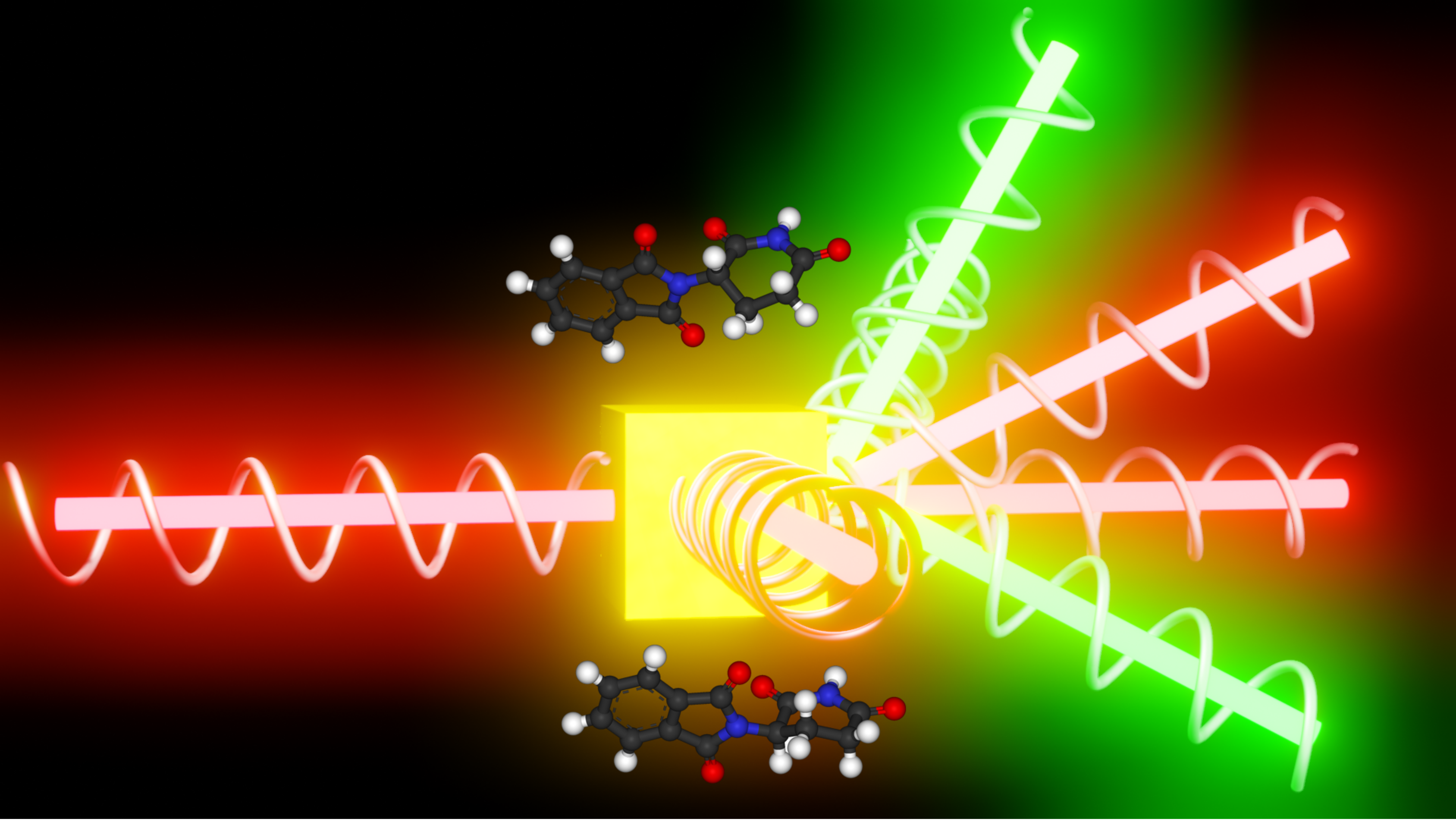
Figure 1: Scattering process in which an incident field with well-defined helicity (red beam with $\sigma=+1$) impinges on an achiral antenna, represented by a glossy cube. Both $\rm{R}$-and-$\rm{S}$ Thalomide enantiomers are also depicted close to the achiral antenna.

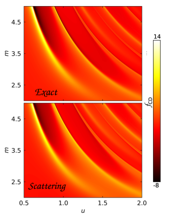
Figure 2: Circular dichroism enhancements for a multipolar sphere under the illumination of a circularly polarized plane-wave. a) $\mathit{f}_{\rm{CD}}$ (exact) and b) $\mathit{f}_{\rm{CD}}-{\tilde{\rm{C}}^{\sigma}_{\rm{int}}}/{\tilde{\rm{C}}^{\sigma}_{\rm{inc}}}$ (scattering). Here $u=x+\delta_{x}$, with $\delta_{x}\ll 1$, being $x=ka$ the optical size and $m$ the index contrast.

Equation (8), together with Eqs. (9)-(12), is the first main result of this paper. These equations describe the integrated CD enhancement in the presence of scatterers of any size and shape under the excitation of fields with well-defined helicity. Our results overcome previous approximations, such as the widely used system of a circularly-polarized plane-wave illuminating dipolar objects Zhang et al. (2017); Yao and Liu (2018); Hanifeh and Capolino (2020); A. Paiva-Marques et al. (2020); Hendry et al. (2012); Solomon et al. (2018); Graf et al. (2019); Garcia-Guirado et al. (2019); Lasa-Alonso et al. (2020); Droulias and Bougas (2020); Mohammadi et al. (2021); Rui et al. (2022). Thus, our findings may find applications in chiral sensing and chiral spectroscopy techniques beyond the current state-of-the-art.

At this point and for didactic purposes, we provide the steps to find $\mathit{f}_{\rm{CD}}$ around any optical antenna, which can be organized as follows:

1. First, we need the solution of the electromagnetic fields under the illumination of a well-defined helicity beam. These can be obtained by any Maxwell’s solver .

2. Then, we project in the far field the exact solution of the electromagnetic fields scattered by the object to obtain the scattering coefficients (see Eq. (9.123) in Jackson’s book in its third edition Jackson (1999)). For convenience, we provide in Appendix C the conversion between our scattering coefficients $a_{lm}$ and $b_{lm}$ to the ones employed in Jackson’s book. Also notice that for spherical objects, we might use Mie’s theory to directly jump to step 3.

3. Finally, we can compute $\mathit{f}_{\rm{CD}}$ via Eq. (8), together with Eqs. (9)-(12).

As an illustrative example of the abovementioned recipe, we depict the exact expression of $\mathit{f}_{\rm{CD}}$ for a sphere sustaining several multipoles under plane-wave illumination (see Fig. 2a)). Moreover, we also depict in Fig. 2b) the scattering contribution to $\mathit{f}_{\rm{CD}}$. That is, $\mathit{f}_{\rm{CD}}-{\tilde{\rm{C}}^{\sigma}_{\rm{int}}}/{\tilde{\rm{C}}^{\sigma}_{\rm{inc}}}$. In fact, we infer, by comparing Fig. 2a) with Fig. 2b), that the exact solution of $\mathit{f}_{\rm{CD}}$ can be fairly approximated to just scattering in near-field, namely, $\mathit{f}_{\rm{CD}}\sim 1+{\tilde{\rm{C}}^{\sigma}_{\rm{sca}}}/{\tilde{\rm{C}}^{\sigma}_{\rm{inc}}}$. Now, we understand the validity of this approximation based on the following facts:

• On mathematical grounds, and according to Eq. (34), it can be checked that $G_{h_{l}h_{l}}\gg|G_{j_{l}h_{l}}|$ for $u<l$. That is, fundamental properties of spherical Bessel functions dictate that the scattering contribution dominates over the interference term for $u<l$.

• On physical grounds, we notice that there are no strong resonances of the $l$-th multipole for $u>l$. For example, dipolar and quadrupolar resonances typically arise for $u<1$ and $1<u<2$, respectively Coe et al. (2022).

Table 1: Analytic expressions for the CD enhancement factor, $\mathit{f}_{\rm{CD}}$, depending on the interaction between an incident plane-wave and an achiral scatterer. Here $a_{lm}$ and $b_{lm}$ denote the electric and magnetic scattering coefficients and $\{G_{h_{l}h_{l}},G_{j_{l}h_{l}}\}$ can be computed from Eq. (34); $\langle\Lambda\rangle$ denotes the electromagnetic helicity expectation value and $\Lambda_{\theta}$ the helicity density; $\sigma_{\rm{sca}}$ and $\sigma_{\rm{ext}}$ are the scattering and extinction cross-sections; and $\lambda$ the radiation wavelength.

Approximation in the calculation of $\mathit{f}_{\rm{CD}}$	Plane wave illumination
Exact multipolar expansion	$\mathit{f}_{\rm{CD}}=1+\sum_{lm}\left(2l+1\right)\left(\text{Re}\{a_{lm}{b_{lm}}^{*}\}G_{h_{l}h_{l}}+\text{Re}\{\left(a_{lm}+b_{lm}\right)G_{j_{l}h_{l}}\}\right)$
Scattering approximation	$\mathit{f}_{\rm{CD}}\sim 1+\sum_{lm}\left(2l+1\right)\text{Re}\{a_{lm}{b_{lm}}^{*}\}G_{h_{l}h_{l}}$
Scattering approximation for arbitrary samples well-described by a single multipolar order $l$	$\mathit{f}_{\rm{CD}}\sim 1+\dfrac{\pi G_{h_{l}h_{l}}}{\lambda^{2}}\langle\Lambda\rangle{\sigma}_{\rm{sca}}\underbrace{\longrightarrow}_{\text{Lossless}}\mathit{f}_{\rm{CD}}\sim 1+\dfrac{\pi G_{h_{l}h_{l}}}{\lambda^{2}}\langle\Lambda\rangle{\sigma}_{\rm{ext}}$
Scattering approximation for cylindrical samples well-described by a single multipolar order $l$	$\mathit{f}_{\rm{CD}}\sim 1+\dfrac{\pi G_{h_{l}h_{l}}}{\lambda^{2}}\Lambda_{\theta}{\sigma}_{\rm{sca}}\underbrace{\longrightarrow}_{\text{Lossless}}\mathit{f}_{\rm{CD}}\sim 1+\dfrac{\pi G_{h_{l}h_{l}}}{\lambda^{2}}\Lambda_{\theta}{\sigma}_{\rm{ext}}$

At this point, we will delve into Eq. (10), which approximates the efficiency of an optical antenna to enhance the $\mathit{f}_{\rm{CD}}$ factor, as it has just been previously explained. In particular, let us examine its physical meaning when just one multipole order (electric and magnetic) contributes to the optical response of the antenna. In this regard, it is essential to note that the one multipole approximation includes the most studied scenario by the nanophotonic community devoted to enhanced chiral sensing: a circularly polarized plane wave incident on dipolar objects Zhang et al. (2017); Yao and Liu (2018); Hanifeh and Capolino (2020); A. Paiva-Marques et al. (2020); Hendry et al. (2012); Solomon et al. (2018); Graf et al. (2019); Garcia-Guirado et al. (2019); Lasa-Alonso et al. (2020); Droulias and Bougas (2020); Mohammadi et al. (2021); Rui et al. (2022). Now, when the scattering can be described by just one multipole order, $l$, Eq. (10) reads

$$\tilde{\rm{C}}^{\sigma}_{\rm{sca}} = \sigma G_{h_{l}h_{l}}\sum_{m=-l}^{m=l}|C^{\sigma}_{lm}|^{2}\text{Re}\{a_{lm}{b_{lm}}^{*}\},$$ (13)

By inspecting Eq. (13), we notice that $\tilde{\rm{C}}^{\sigma}_{\rm{sca}}$ is proportional to the interference between the electric and magnetic scattering coefficients $\text{Re}\{a_{lm}{b_{lm}}^{*}\}$. Now, let us introduce the normalized (and unit-less) electromagnetic helicity expectation value, which reads Olmos-Trigo et al. (2020b, c); Lasa-Alonso et al. (2022)

$$\langle\Lambda\rangle=\frac{\int_{\Omega}\left({|{\bf E}^{\sigma+}_{\rm{sca}}}|^{2}-{|{\bf E}^{\sigma-}_{\rm{sca}}}|^{2}\right)\;d\Omega}{\int_{\Omega}\left({|{\bf E}^{\sigma+}_{\rm{sca}}}|^{2}+{|{\bf E}^{\sigma-}_{\rm{sca}}}|^{2}\right)\;d\Omega}.$$ (14)

Computing $\langle\Lambda\rangle$ in the case in which the optical response can be described by a single multipolar order $l$ Olmos-Trigo et al. (2020b, c); Lasa-Alonso et al. (2022), we obtain

$${\langle\Lambda\rangle}=2\sigma\frac{\sum_{m}|C^{\sigma}_{lm}|^{2}\text{Re}\{a_{lm}{b_{lm}}^{*}\}}{\sum_{m}|C^{\sigma}_{lm}|^{2}\left(|a_{lm}|^{2}+|b_{lm}|^{2}\right)}=\frac{\sigma\sum_{m}|C^{\sigma}_{lm}|\text{Re}\{a_{lm}{b_{lm}}^{*}\}}{k^{2}\sigma_{\rm{sca}}},$$ (15)

where $\sigma_{\rm{sca}}$ is the scattering cross section Bohren and Huffman (2008). At this point, we notice that the expression for $\tilde{\rm{C}}^{\sigma}_{\rm{sca}}$ resembles $\langle\Lambda\rangle$. In fact and without loss of generality, we can write $\tilde{\rm{C}}^{\sigma}_{\rm{sca}}={G_{h_{l}h_{l}}}\langle\Lambda\rangle k^{2}\sigma_{\rm{sca}}$. As a result, $\mathit{f}_{\rm{CD}}$ yields

$$\mathit{f}_{\rm{CD}}\sim 1+\frac{{\tilde{\rm{C}}^{\sigma}_{\rm{sca}}}}{\tilde{\rm{C}}^{\sigma}_{\rm{inc}}}=1+\frac{{{G_{h_{l}h_{l}}}\langle\Lambda\rangle{k^{2}\sigma_{\rm{sca}}}}}{\tilde{\rm{C}}^{\sigma}_{\rm{inc}}}.$$ (16)

This is another significant result of the present work. We have linked the averaged optical chirality associated with scattered fields, $\tilde{\rm{C}}^{\sigma}_{\rm{sca}}$, which is usually computed in the near-field, with quantities that can be evaluated or measured in far-field, i.e. the helicity expectation value, $\langle\Lambda\rangle$ and the scattering cross-section, ${{\sigma}_{\rm{sca}}}$. In addition, and for helicity-preserving objects, $\langle\Lambda\rangle\sim 1$, the averaged optical chirality associated with scattered fields is simply given by the scattering cross-section. That is, $\tilde{\rm{C}}^{\sigma}_{\rm{sca}}\sim G_{h_{l}h_{l}}k^{2}{\sigma}_{\rm{sca}}$. It is also essential to notice that, for both lossless and helicity-preserving objects, $\tilde{\rm{C}}^{\sigma}_{\rm{sca}}\sim G_{h_{l}h_{l}}k^{2}{\sigma}_{\rm{ext}}$, with ${\sigma}_{\rm{ext}}={\sigma}_{\rm{sca}}$, ${\sigma}_{\rm{ext}}$ being the extinction cross-section Bohren and Huffman (2008). That is, the CD enhancement captured by the $\mathit{f}_{\rm{CD}}$ factor is related to a single measurement of the extincted power in the forward direction whenever $\langle\Lambda\rangle\sim 1$. The relation between $\mathit{f}_{\rm{CD}}$ and ${\sigma}_{\rm{ext}}$ for helicity-preserving achiral objects greatly reduces eventual experimental and numerical calculations devoted to enhanced chiral sensing.

So far, we have shown an alternative way to infer local CD enhancements in the near-field limit by computing far-field magnitudes such as the helicity expectation value, the scattering cross-section, or the extinction cross-section. In particular, a scenario of major interest for the purpose of enhanced chiral detection occurs when the antenna preserves the helicity of the incident illumination, i.e. whenever $\langle\Lambda\rangle\sim 1$. These objects satisfy $|{\bf E}^{\sigma\sigma^{\prime}}_{\rm{sca}}({\bf r})|\sim 0$ for $\sigma\neq\sigma^{\prime}$. This phenomenon is desirable since the local sign of optical chirality is preserved. Experimentally, identifying helicity-preserving scatterers requires measuring the polarization of all the scattered field components, something which is not feasible in practice. Thus, our question is: can we infer the helicity expectation value, $\langle\Lambda\rangle$, from a single measurement in the far-field? In the last part of this work, we will discuss scenarios in which the helicity density at a given scattering angle can be identical to its expected value. In particular, we will focus on cylindrically symmetric scatterers which preserve the total angular momentum in the incident direction ($m=m^{\prime}$) and whose optical response can be well-described by a single multipolar order ($l=l^{\prime}$), e.g., nanodisks at normal incidence or spherical particles under the illumination of tightly-focused Laguerre-Gaussian beams Sanz-Fernández et al. (2021).

Mathematically, we can express the aforementioned condition as ${\langle\Lambda\rangle}=\Lambda_{\theta}$, where $\Lambda_{\theta}$ denotes the helicity density at an angle $\theta$, where $\theta$ is the scattering angle. After some algebra (see Appendix D), we obtain:

$$P^{m}_{l}(\cos\theta)\frac{\partial P^{m}_{l}(\cos\theta)}{\partial\cos\theta}=0~{}~{}~{}\Longrightarrow~{}~{}~{}{\langle\Lambda\rangle}=\Lambda_{\theta},$$ (17)

where $P^{m}_{l}(\cos\theta)$ are the associated Legendre Polynomials Jackson (1999). This is another key result of the present work. The helicity expectation value can indeed be computed from a single measurement of the helicity density at a specific angle $\theta$. Our result implies that for a cylindrically symmetric scatterer whose response can be well-described by a single multipolar order, $l$, if we excite it with an illumination with a fixed total angular momentum, $m$, Eq. (17) specifies the angle at which the helicity density is equal to its expected value. For instance, if we consider the typical case of a cylindrically symmetric dipolar target ($l=1$) under a circularly polarized plane-wave illumination ($m=\pm 1$), Eq. (17) yields that the angle we should look at is $\theta=\pi/2$. That is, the expectation value of the electromagnetic helicity can be inferred from a single measurement at the right angle. Thus, and according to Eq. (16), for lossless and cylindrically symmetric targets, we can infer the $\mathit{f}_{\rm{CD}}$ factor by just considering two far-field measurements: extinction cross-section, in the forward direction, and helicity density, at an angle $\theta$ specified by Eq. (17) .

Table 1 resumes the main results of this work, particularized for plane-wave illumination, as it is the most common external excitation for enhanced chiral sensing to date. In short, we have derived an exact multipole expansion of the integrated CD enhancement factor, $\mathit{f}_{\rm{CD}}$, for scatterers of any form and shape under general illumination conditions. In addition, we have established a roadmap to infer local CD enhancements from far-field measurements. That is, $\mathit{f}_{\rm{CD}}$ can be extracted by calculating the helicity expectation value and the scattering cross section, two Stokes parameters that can be evaluated in the far-field limit. Finally, we have shown an even more practical route to deduce $\mathit{f}_{\rm{CD}}$ for cylindrically symmetric objects by means of measuring the extinction cross-section and the local density of electromagnetic helicity at specific angles. Our results pave the way for experimental verification and characterization of building blocks for CD enhancement from far-field measurements, and thus, may give rise to novel developments in the field of chiral light-matter interactions.

Appendix A Multipolar electromagnetic fields in a well-defined helicity basis

A.1 Incident electromagnetic fields

To start with the calculation of the surface-enhanced circular dichroism (CD), we need first to write down the electromagnetic fields. The most generic expression of the incident electromagnetic fields are given by

$${\bf E}_{\rm{inc}}({\bf r}) = \sum_{l=0}^{\infty}\sum_{m=-l}^{+l}g^{e}_{lm}\bm{N}^{j}_{lm}({\bf r})+g^{m}_{lm}\bm{M}^{j}_{lm}({\bf r}),$$ (18)

$${\rm i}Z{\bf H}_{\rm{inc}}({\bf r}) = \sum_{l=0}^{\infty}\sum_{m=-l}^{+l}g^{e}_{lm}\bm{M}^{j}_{lm}({\bf r})+g^{m}_{lm}\bm{N}^{j}_{lm}({\bf r}),$$ (19)

where $g^{e}_{lm}$ and $g^{m}_{lm}$ stands for the incident electric and magnetic beam’s shape coefficients, respectively, and

$${\bm{M}}^{j}_{lm}({\bf r})=j_{l}(kr)\bm{X}_{lm}({\bf r}),\qquad{\bm{N}}^{j}_{lm}({\bf r})=\frac{\bm{\nabla}\times{\bm{M}}^{j}_{lm}({\bf r})}{k},\qquad\bm{X}_{lm}({\bf r})=\frac{{\bf{L}}Y_{lm}(\theta,\varphi)}{\sqrt{l(l+1)}}.$$ (20)

Here $\bm{M}^{j}_{lm}({\bf r})$ and $\bm{N}^{j}_{lm}({\bf r})$ are (incident) Hansen’s multipoles Jackson (1999), $j_{l}(kr)$ are the spherical Bessel functions, $k$ being the radiation wavelength, and ${\bf r}$ the observation point. Moreover, $Y_{lm}(\theta,\varphi)$ are the spherical harmonics, $\theta$ and $\varphi$ being the polar and azimuthal angles, and ${\bf{L}}=\left\{-{\rm i}{\bf r}\times\bm{\nabla}\right\}$ is the total angular momentum operator. At this point, let us consider an arbitrary incident electromagnetic field with well-defined helicity, $\sigma=\pm 1$. Mathematically, we can write this well-defined helicity field as

$${\bf E}^{\sigma}_{\rm{inc}}({\bf r}) = \frac{{\bf E}_{\rm{inc}}({\bf r})+\sigma{\rm i}Z{\bf H}_{\rm{inc}}({\bf r})}{2}=\sum_{l=0}^{\infty}\sum_{m=-l}^{+l}\left(\frac{{g^{e}_{lm}+\sigma g^{m}_{lm}}}{\sqrt{2}}\right)\left(\frac{{\bm{N}}^{j}_{lm}({\bf r})+\sigma{\bm{M}}^{j}_{lm}({\bf r})}{\sqrt{2}}\right)=\sum_{l=0}^{\infty}\sum_{m=-l}^{+l}C_{lm}^{\sigma}\bm{\Psi}_{lm}^{\sigma}({\bf r}),$$ (21)

where

$$C_{lm}^{\sigma}=\frac{{g^{e}_{lm}+\sigma g^{m}_{lm}}}{\sqrt{2}}, \bm{\Psi}_{lm}^{\sigma}({\bf r})=\frac{{\bm{N}}^{j}_{lm}({\bf r})+\sigma{\bm{M}}^{j}_{lm}({\bf r})}{\sqrt{2}}.$$ and (22)

Let us recall that the multipoles $\bm{\Psi}_{lm}^{\sigma}({\bf r})$ are eigenvectors of the squared angular momentum $L^{2}$, the projection of the angular momentum on one direction, $L_{z}$, and helicity $\bm{\Lambda}=(1/k)\nabla\times$ Fernandez-Corbaton et al. (2013) with eigenvalues $l(l+1)$, $m$, $\sigma$, respectively.

A.2 Scattered and total electromagnetic fields

At this point, let us consider the scattered electromagnetic fields. The most generic expression of these fields is given by

$${\bf E}^{\sigma}_{\rm{sca}}({\bf r}) = \sum_{l=0}^{\infty}\sum_{m=-l}^{+l}a^{\sigma}_{lm}\bm{N}^{h}_{lm}({\bf r})+b^{\sigma}_{lm}\bm{M}^{h}_{lm}({\bf r}),$$ (23)

$${\rm i}Z{\bf H}^{\sigma}_{\rm{sca}}({\bf r}) = \sum_{l=0}^{\infty}\sum_{m=-l}^{+l}a^{\sigma}_{lm}\bm{M}^{h}_{lm}({\bf r})+b^{\sigma}_{lm}\bm{N}^{h}_{lm}({\bf r}),$$ (24)

where $a^{\sigma}_{lm}$ and $b^{\sigma}_{lm}$ stand for the electric and magnetic scattering coefficients, respectively. Notice that $a^{\sigma}_{lm}$ and $b^{\sigma}_{lm}$ depend on the incident illumination. As a result, we have explicitly indicated the $\sigma$-dependency. Moreover,

$${\bm{M}}^{h}_{lm}({\bf r})=h_{l}(kr)\bm{X}_{lm}({\bf r}),\qquad{\bm{N}}^{h}_{lm}({\bf r})=\frac{\bm{\nabla}\times{\bm{M}}^{h}_{lm}({\bf r})}{k},$$ (25)

where $\bm{M}^{h}_{lm}({\bf r})$ and $\bm{N}^{h}_{lm}({\bf r})$ are (scattered) Hansen’s multipoles Jackson (1999) and $h_{l}(kr)$ are the spherical Hankel functions. Following the steps done in Eq. (21), the electric field reads as

$${\bf E}^{\sigma\sigma^{\prime}}_{\rm{sca}}({\bf r})=\frac{{\bf E}^{\sigma}_{\rm{sca}}({\bf r})+\sigma^{\prime}{\rm i}Z{\bf H}^{\sigma}_{\rm{sca}}({\bf r})}{2} = \sum_{l=0}^{\infty}\sum_{m=-l}^{+l}\left(\frac{{a^{\sigma}_{lm}+\sigma^{\prime}b^{\sigma}_{lm}}}{\sqrt{2}}\right)\left(\frac{{\bm{N}}^{h}_{lm}({\bf r})+\sigma^{\prime}{\bm{M}}^{h}_{lm}({\bf r})}{\sqrt{2}}\right)=\sum_{l=0}^{\infty}\sum_{m=-l}^{+l}D_{lm}^{\sigma\sigma^{\prime}}\bm{\Phi}_{lm}^{\sigma^{\prime}}({\bf r}),$$ (26)

where

$$D_{lm}^{\sigma\sigma^{\prime}}=\frac{{a^{\sigma}_{lm}+\sigma^{\prime}b^{\sigma}_{lm}}}{\sqrt{2}}, \bm{\Phi}_{lm}^{\sigma^{\prime}}({\bf r})=\frac{{\bm{N}}^{h}_{lm}({\bf r})+\sigma^{\prime}{\bm{M}}^{h}_{lm}({\bf r})}{\sqrt{2}}.$$ and (27)

At this stage, let us write down the relation between the incident and scattering amplitudes. These are given by Cramer’s rule of the tangential Maxwell boundary conditions Jackson (1999), $a^{\sigma}_{lm}=a_{lm}g^{e}_{lm}$ and $b^{\sigma}_{lm}=b_{lm}g^{m}_{lm}$ where $a_{lm}$ and $b_{lm}$ are the so-called electric and magnetic scattering coefficients, respectively. Notice $a_{lm}$ and $b_{lm}$ do not depend on the incident illumination but on the optical properties and geometry of the target, e.g., the electric and magnetic Mie coefficients. Now, and since we are dealing with a well-defined helicity field, we can notice from Eq. (21) that $g^{e}_{lm}=\sigma g^{m}_{lm}$. Accordingly, we can write

$$a^{\sigma}_{lm}=a_{lm}\left(\frac{C^{\sigma}_{lm}}{\sqrt{2}}\right), b^{\sigma}_{lm}=\sigma b_{lm}\left(\frac{C^{\sigma}_{lm}}{\sqrt{2}}\right).$$ (28)

Now, by inserting Eq. (28) into the left side of Eq. (27), we arrive to

$$D^{\sigma\sigma^{\prime}}_{lm}=C^{\sigma}_{lm}\frac{\left({a_{lm}+\sigma\sigma^{\prime}b_{lm}}\right)}{2}.$$ (29)

From now on, this will be our choice for the representation of the scattered coefficients. To conclude Appendix A, let us write the total electromagnetic fields. These are given by the additive sum of the incident and scattered electromagnetic fields. Hence, by taking into account both Eq. (21) and Eq. (26), we can straightforwardly write,

$${\bf E}^{\sigma}_{\rm{tot}}({\bf r}) = \sum_{\sigma^{\prime}=\pm 1}{\bf E}^{\sigma\sigma^{\prime}}_{\rm{tot}}({\bf r}),\qquad{\rm i}Z{\bf H}^{\sigma}_{\rm{tot}}({\bf r})=\sum_{\sigma^{\prime}=\pm 1}\sigma^{\prime}{\bf E}^{\sigma\sigma^{\prime}}_{\rm{tot}}({\bf r}),$$ (30)

with

$${\bf E}^{\sigma\sigma^{\prime}}_{\rm{tot}}({\bf r}) = {\bf E}^{\sigma\sigma^{\prime}}_{\rm{sca}}({\bf r})+{\bf E}^{\sigma}_{\rm{inc}}({\bf r})\delta_{\sigma\sigma^{\prime}},$$ (31)

where $\delta_{\sigma\sigma^{\prime}}$ is a Kronecker delta. Next, we will use the orthogonality expressions that satisfy both the incident and scattered electromagnetic fields to compute the exact multipolar expansion of the CD enhancement factor.

Appendix B An exact multipolar expansion of $f_{\rm{CD}}$ beyond the plane-wave picture

B.1 An exact multipolar expansion of $f_{\rm{CD}}$: Orthogonality relations of well-defined helicity multipoles

To derive an exact multipolar expansion of the CD enhancement factor, $\mathit{f}_{\rm{CD}}$, beyond the plane-wave picture, we need to know the orthogonality relations that satisfy both incident and scattered electromagnetic fields over an integrating sphere surrounding the object under illumination. To that end, we need first to calculate the set of orthogonality relations that fulfill the multipoles with well-defined helicity. That is, we need the orthogonality relations between incident $\{\bm{\Psi}_{lm}^{\sigma},\bm{\Psi}_{l^{\prime}m^{\prime}}^{\sigma}\}$, interference $\{\bm{\Psi}_{lm}^{\sigma},\bm{\Phi}_{l^{\prime}m^{\prime}}^{\sigma}\}$, and scattering $\{\bm{\Phi}_{lm}^{\sigma},\bm{\Phi}_{l^{\prime}m^{\prime}}^{\sigma}\}$ terms, according to Eq. (7). Fortunately, all these relations can be derived from Jackson’s third edition book. Let us start this section by transcribing Eq. $10.48$ that can be found on page $472$ of Ref. Jackson (1999):

$$\int_{\Omega}{N^{f}_{lm}}^{*}\cdot N^{g}_{l^{\prime}m^{\prime}}d\Omega=\delta_{ll^{\prime}}\delta_{mm^{\prime}}\left(f^{*}_{l}(u)g_{l}(u)+\frac{1}{u^{2}}\frac{\partial}{\partial u}\left(uf^{*}_{l}(u)\frac{\partial}{\partial u}\left(ug_{l}(u)\right)\right)\right), \int_{\Omega}{M^{f}_{lm}}^{*}\cdot M^{g}_{l^{\prime}m^{\prime}}d\Omega=f^{*}_{l}(u)g_{l}(u)\delta_{ll^{\prime}}\delta_{mm^{\prime}}.$$ (32)

Here $u=kr$ denotes the optical radius of the integrating sphere and $\{\delta_{ll^{\prime}},\delta_{mm^{\prime}}\}$ are Kronecker deltas. Notice that $\{f_{l}(u),g_{l}(u)\}$ denote either Bessel or Hankel spherical functions, namely, $j_{l}(u)$ and $h_{l}(u)$ Jackson (1999), depending on the nature of the field: incident or scattered, respectively.

At this point, we have already learned that multipoles with well-defined helicity $\{\bm{\Psi}_{lm}^{\sigma},\bm{\Phi}_{lm}^{\sigma}\}$ are constructed by a linear combination of the Hansel multipoles (see the right side of Eq. (22) and Eq. (27) . As a result, we can write from Eq. (32)

$$\int_{\Omega}({\bm{\Psi}^{\sigma}_{l^{\prime}m^{\prime}}})^{*}\cdot\bm{\Psi}_{lm}^{\sigma}\;d\Omega=G_{j_{l}j_{l}}\delta_{ll^{\prime}}\delta_{mm^{\prime}}, \int_{\Omega}({\bm{\Phi}^{\sigma}_{l^{\prime}m^{\prime}}})^{*}\cdot{\bm{\Phi}^{\sigma}_{lm}}\;d\Omega=G_{h_{l}h_{l}}\delta_{ll^{\prime}}\delta_{mm^{\prime}}, \int_{\Omega}({\bm{\Psi}^{\sigma}_{l^{\prime}m^{\prime}}})^{*}\cdot\bm{\Phi}_{lm}^{\sigma}\;d\Omega=G_{j_{l}h_{l}}\delta_{ll^{\prime}}\delta_{mm^{\prime}},$$ (33)

with

$$G_{f_{l}g_{l}}=\frac{1}{2}\left[2f^{*}_{l}(u)g_{l}(u)+\frac{1}{u^{2}}\frac{\partial}{\partial u}\left(uf^{*}_{l}(u)\frac{\partial}{\partial u}\left(ug_{l}(u)\right)\right)\right].$$ (34)

Now, we can re-write Eq. (34) to get rid of second derivatives by making use of fundamental properties of the Ricatti-Bessel functions Watson (1995). In particular, we can write,

$$G_{j_{l}j_{l}}=\frac{1}{2}\left[j^{2}_{l}(u)\left(1+\frac{l(l+1)}{u^{2}}\right)+\frac{1}{u^{2}}\left(\frac{\partial}{\partial u}\left(uj_{l}(u)\right),\right)^{2}\right] G_{h_{l}h_{l}}=\frac{1}{2}\left[|h_{l}(u)|^{2}\left(1+\frac{l(l+1)}{u^{2}}\right)+\frac{1}{u^{2}}\left|\frac{\partial}{\partial u}\left(uh_{l}(u)\right)\right|^{2}\right],$$ (35)

$$G_{j_{l}h_{l}}=\frac{1}{2}\left[j_{l}(u)h_{l}(u)\left(1+\frac{l(l+1)}{u^{2}}\right)+\frac{1}{u^{2}}\left(\frac{\partial}{\partial u}\left(uj_{l}(u)\right)\frac{\partial}{\partial u}\left(uh_{l}(u)\right)\right)\right],$$ (36)

where $\frac{\partial}{\partial u}\left(uf_{l}(u)\right))=uf_{l-1}(u)-lf_{l}(u)$ is satisfied for $f(u)=\{j_{l}(u),h_{l}(u)\}$.

B.2 An exact multipolar expansion of $f_{\rm{CD}}$: From the helicity basis to the standard electric and magnetic multipolar expansion

At this stage, we have all ingredients to calculate the exact multipolar expansion of $f_{\rm{CD}}$. The starting point of this section will be Eq. (7). According to Eq. (7), we need the orthogonality relations that satisfy the Rieman-Silberstein representation of the incident and scattered electromagnetic fields:

$$\tilde{\rm{C}}^{\sigma}_{\rm{inc}} = \int_{\Omega}{\rm{C}}^{\sigma}_{\rm{inc}}({\bf r})d\Omega=\int_{\Omega}\sigma|{\bf E}^{\sigma}_{\rm{inc}}({\bf r})|^{2}d\Omega,$$ (37)

$$\tilde{\rm{C}}^{\sigma}_{\rm{sca}} = \int_{\Omega}{\rm{C}}^{\sigma}_{\rm{sca}}({\bf r})d\Omega=\int_{\Omega}|{\bf E}^{\sigma+}_{\rm{sca}}({\bf r})|^{2}-|{\bf E}^{\sigma-}_{\rm{sca}}({\bf r})|^{2}d\Omega,$$ (38)

$${\rm{C}}^{\sigma}_{\rm{int}} = \int_{\Omega}\tilde{{\rm{C}}}^{\sigma}_{\rm{int}}({\bf r})d\Omega=2\sigma\int_{\Omega}\text{Re}\{{{\bf E}^{\sigma}_{\rm{inc}}}^{*}({\bf r})\cdot{{\bf E}^{\sigma\sigma}_{\rm{sca}}}({\bf r})\}d\Omega.$$ (39)

These orthogonality relations can be computed by combining Eq. (21) and Eq. (26) with Eq. (33). In fact and after some algebraic manipulations, it can be shown that

$$\tilde{\rm{C}}^{\sigma}_{\rm{inc}}=\sigma\sum_{lm}|C^{\sigma}_{lm}|^{2}G_{j_{l}j_{l}}, \tilde{\rm{C}}^{\sigma}_{\rm{sca}}=\sum_{lm}\left(|D^{\sigma+}_{lm}|^{2}-|D^{\sigma-}_{lm}|^{2}\right)G_{h_{l}h_{l}}, \tilde{{\rm{C}}}^{\sigma}_{\rm{int}}=2\sigma\sum_{lm}\text{Re}\{{C^{\sigma}_{lm}}^{*}D^{\sigma\sigma}_{lm}G_{j_{l}h_{l}}\}.$$ (40)

Now, let us insert Eq. (29) into Eq. (40) to obtain a closed-relation of the optical chirality enhancements in terms of the electric and magnetic scattering coefficients. After some algebra, we arrive to

$$\mathit{f}_{\rm{CD}}=1+\frac{\tilde{\rm{C}}^{\sigma}_{\rm{sca}}+\tilde{\rm{C}}^{\sigma}_{\rm{int}}}{\tilde{\rm{C}}^{\sigma}_{\rm{inc}}},$$ (41)

with

$$\tilde{\rm{C}}^{\sigma}_{\rm{inc}}=\sigma\sum_{lm}|C^{\sigma}_{lm}|^{2}G_{j_{l}j_{l}}, \tilde{\rm{C}}^{\sigma}_{\rm{sca}}=\sigma\sum_{lm}|C^{\sigma}_{lm}|^{2}\text{Re}\{a_{lm}{b_{lm}}^{*}\}G_{h_{l}h_{l}}, \tilde{\rm{C}}^{\sigma}_{\rm{int}}=\sigma\sum_{lm}|C^{\sigma}_{lm}|^{2}\text{Re}\{\left(a_{lm}+b_{lm}\right)G_{j_{l}h_{l}}\}.$$ (42)

Appendix C Conversion from our conventions to those in Jackson’s book

The multipolar expansion of the scattered electromagnetic fields provided in Jackson’s book reads as Jackson (1999)

$${\bf E}^{\rm{Jack}}_{\rm{sca}} = Z\sum_{l=0}^{\infty}\sum_{m=-l}^{+l}{\rm i}a_{E}(l,m)\bm{N}^{h}_{lm}({\bf r})+a_{M}(l,m)\bm{M}^{h}_{lm}({\bf r}),$$ (43)

$${\rm i}Z{\bf H}^{\rm{Jack}}_{\rm{sca}} = Z\sum_{l=0}^{\infty}\sum_{m=-l}^{+l}{\rm i}a_{E}(l,m)\bm{M}^{h}_{lm}({\bf r})+a_{M}(l,m)\bm{N}^{h}_{lm}({\bf r}).$$ (44)

Now, by inspecting Eqs. (43)-(44), we notice that the conversion from our conventions to those in Jackson’s book are given by

$$a_{lm}=\sqrt{2}{\rm i}Z\left[\frac{a_{E}(l,m)}{C^{\sigma}_{lm}}\right], b_{lm}=\sqrt{2}\sigma Z\left[\frac{a_{M}(l,m)}{C^{\sigma}_{lm}}\right].$$ (45)

where $Z=\mu/\epsilon$ is the medium impedance. Notice that the electric and magnetic coefficients, provided in Jackson’s book, can be computed by conventional far-field projections of the scattered electromagnetic fields (see Eq. (9.123) in Ref. Jackson (1999)). For completeness, we transcribe these expressions,

$$Za_{E}(l,m)h_{l}(kr)=-\frac{k}{\sqrt{l(l+1)}}\int Y^{*}_{lm}(\theta,\varphi){\bf r}\cdot{\bf E}^{\rm{Jack}}_{\rm{sca}}, a_{M}(l,m)h_{l}(kr)=\frac{k}{\sqrt{l(l+1)}}\int Y^{*}_{lm}(\theta,\varphi){\bf r}\cdot{\bf H}^{\rm{Jack}}_{\rm{sca}}.$$ (46)

Appendix D Extracting the helicity expectation value from a single measurement of its local density

In this Appendix, we derive the condition given in Eq. (17), that relates the local density of helicity at a certain angle, $\Lambda_{\theta,\phi}$, with the helicity expectation value, $\langle\Lambda\rangle$. For that aim, we should first define the local density of helicity, which we consider to be given in far-field by:

$$\Lambda_{\theta,\varphi}\equiv\lim_{kr\rightarrow\infty}\frac{|\mathbf{E}^{\sigma+}_{\rm{sca}}(r,\theta,\varphi)|^{2}-|\mathbf{E}^{\sigma-}_{\rm{sca}}(r,\theta,\varphi)|^{2}}{|\mathbf{E}^{\sigma+}_{\rm{sca}}(r,\theta,\varphi)|^{2}+|\mathbf{E}^{\sigma-}_{\rm{sca}}(r,\theta,\varphi)|^{2}},$$ (47)

where $\mathbf{E}^{\sigma\sigma^{\prime}}_{\rm{sca}}(r,\theta,\varphi)$ is the scattered field written in terms of electromagnetic modes with well-defined helicity. From Eq. (47), we notice that we require the asymptotic behavior of $\mathbf{E}^{\sigma\sigma^{\prime}}_{\rm{sca}}(r,\theta,\varphi)$ in the far-field limit. For that aim, we need first to calculate how Hansel multipoles behave in the far-field limit. After some algebra, we arrive to

$$\lim_{kr\rightarrow\infty}\bm{N}^{h}_{lm}({\bf r})=-\frac{e^{ikr}}{kr}\frac{(-i)^{l+1}}{\sqrt{l(l+1}}\bm{\xi}_{lm}(\theta,\varphi), \lim_{kr\rightarrow\infty}\bm{M}^{h}_{lm}({\bf r})=-\frac{e^{ikr}}{kr}\frac{(-i)^{l+1}}{\sqrt{l(l+1}}i\bm{\eta}_{lm}(\theta,\varphi),$$ (48)

where $\bm{\xi}_{lm}(\theta,\varphi)=r\nabla Y_{lm}(\theta,\varphi)$ and $\bm{\eta}_{lm}(\theta,\varphi)=\hat{r}\times\bm{\xi}_{lm}(\theta,\varphi)$. Now, the far-field expression of the electromagnetic field scattered by an arbitrary sample can be computed Carrascal et al. (1991):

$$\mathbf{E}^{\sigma\sigma^{\prime}}_{\rm{sca}}(r,\theta,\varphi)=-\frac{e^{ikr}}{kr}\sum_{lm}(-i)^{l+1}\frac{C_{lm}^{\sigma}}{\sqrt{2l(l+1)}}\left[\frac{a_{lm}+\sigma\sigma^{\prime}b_{lm}}{\sqrt{2}}\right]\left[\frac{\bm{\xi}_{lm}+i\sigma^{\prime}\bm{\eta}_{lm}}{\sqrt{2}}\right].$$ (49)

Substituting the scattered field in Eq. (49) into the expression of the helicity density given by Eq. (47), we obtain for fixed $l$ and $m$ values:

$$\Lambda_{\theta}=2\sigma\frac{\text{Re}\left(a_{lm}{b_{lm}}^{*}\right)\left[|\bm{\xi}_{lm}|^{2}+|\bm{\eta}_{lm}|^{2}\right]-\left[|a_{lm}|^{2}+|b_{lm}|^{2}\right]\text{Im}\left(\bm{\xi}_{lm}^{*}\cdot\bm{\eta}_{lm}\right)}{\left[|a_{lm}|^{2}+|b_{lm}|^{2}\right]\left[|\bm{\xi}_{lm}|^{2}+|\bm{\eta}_{lm}|^{2}\right]-4\text{Re}\left(a_{lm}{b_{lm}}^{*}\right)\text{Im}\left(\bm{\xi}_{lm}^{*}\cdot\bm{\eta}_{lm}\right)}.$$ (50)

The type of scatterers which may be described by fixed $l$ and $m$ values are cylindrically symmetric particles, illuminated by a beam with a well-defined angular momentum, $m$, and with a non multipolar response. Due to the cylindrical symmetry of the scatterers, helicity density cannot depend on $\varphi$ variable. This is the reason why we have chosen to write helicity density as $\Lambda_{\theta}$ in Eq. (50). Crucially, it can be checked that whenever $\text{Im}\left(\bm{\xi}_{lm}^{*}\cdot\bm{\eta}_{lm}\right)=0$, one recovers the expression of the helicity expectation value, i.e.

$$\text{Im}\left(\bm{\xi}_{lm}^{*}\cdot\bm{\eta}_{lm}\right)=0~{}~{}~{}\Longrightarrow~{}~{}~{}\Lambda_{\theta}=\langle\Lambda\rangle=2\sigma\frac{\text{Re}\left(a_{lm}{b_{lm}}^{*}\right)}{|a_{lm}|^{2}+|b_{lm}|^{2}}.$$ (51)

Importantly, the condition $\text{Im}\left(\bm{\xi}_{lm}^{*}\cdot\bm{\eta}_{lm}\right)=0$ is purely geometrical, i.e. does not depend on the particular response of the scatterer. This fact makes the expression completely general and applicable to any type of cylindrical sample whose response is well-described by a fixed $l$. Thus, for this type of scatterers, there are locations in the far-field at which the helicity density is equal to the helicity expectation value.

The specific sites at which $\langle\Lambda\rangle=\Lambda_{\theta}$ are obtained by finding the solutions to the equation $\text{Im}\left(\bm{\xi}_{lm}^{*}\cdot\bm{\eta}_{lm}\right)=0$. More explicitly, we have that the vector and scalar spherical harmonics are written as:

$$\bm{\xi}_{lm}(\theta,\varphi) =\frac{\partial Y_{lm}(\theta,\varphi)}{\partial\theta}\hat{u}_{\theta}+\frac{1}{\sin\theta}\frac{\partial Y_{lm}(\theta,\varphi)}{\partial\varphi}\hat{u}_{\varphi}$$ (52)

$$\bm{\eta}_{lm}(\theta,\varphi) =\frac{\partial Y_{lm}(\theta,\varphi)}{\partial\theta}\hat{u}_{\varphi}-\frac{1}{\sin\theta}\frac{\partial Y_{lm}(\theta,\varphi)}{\partial\varphi}\hat{u}_{\theta}$$ (53)

$$Y_{lm}(\theta,\varphi) =\sqrt{\frac{2l+1}{4\pi}\frac{(l-m)!}{(l+m)!}}P_{l}^{m}(\cos\theta)e^{im\varphi},$$ (54)

where $P_{l}^{m}(\cos\theta)$ are the associated Legendre polynomials. With the definitions above it is straightforward to check that

$$P_{l}^{m}(\cos\theta)\frac{\partial P_{l}^{m}(\cos\theta)}{\partial\cos\theta}=0~{}~{}~{}\Longrightarrow~{}~{}~{}\text{Im}\left(\bm{\xi}_{lm}^{*}\cdot\bm{\eta}_{lm}\right)=0.$$ (55)

In conclusion, for fixed values of $l$ and $m$, there is an angle $\theta$, given by the transcendental equation above, at which the helicity density, $\Lambda_{\theta}$, is equal to the helicity expectation value, $\langle\Lambda\rangle$.

References

Watson (2012)J. Watson, The double helix (Hachette UK, 2012).
McBride (1961)W. G. McBride, Lancet 2, 90927
(1961).
Lenz and Knapp (1962)W. Lenz and K. Knapp, Archives of
Environmental Health: An International Journal 5, 14 (1962).
Calkin (1965)M. Calkin, Am. J.
Phys 33, 958 (1965).
Yu and Capasso (2014)N. Yu and F. Capasso, Nature materials 13, 139 (2014).
Wen et al. (2016)D. Wen, S. Chen, F. Yue, K. Chan, M. Chen, M. Ardron, K. F. Li,
P. W. H. Wong, K. W. Cheah, E. Y. B. Pun, et al., Advanced Optical Materials 4, 321 (2016).
Abendroth et al. (2020)J. M. Abendroth, M. L. Solomon, D. R. Barton III, M. S. El Hadri, E. E. Fullerton, and J. A. Dionne, Advanced Optical Materials 8, 2001420 (2020).
Zhang et al. (2020)C. Zhang, G. Wang,
H.-X. Xu, X. Zhang, and H.-P. Li, Advanced Optical Materials 8, 1901719 (2020).
Zambrana-Puyalto and Bonod (2016)X. Zambrana-Puyalto and N. Bonod, Nanoscale 8, 10441
(2016).
García-Etxarri and Dionne (2013)A. García-Etxarri and J. A. Dionne, Physical Review B 87, 235409 (2013).
Fan and Govorov (2010)Z. Fan and A. O. Govorov, Nano
letters 10, 2580
(2010).
García-Guirado et al. (2018)J. García-Guirado, M. Svedendahl, J. Puigdollers, and R. Quidant, Nano
letters 18, 6279
(2018).
Poulikakos et al. (2018)L. V. Poulikakos, P. Thureja,
A. Stollmann, E. De Leo, and D. J. Norris, Nano letters 18, 4633 (2018).
García-Etxarri et al. (2011)A. García-Etxarri, R. Gómez-Medina, L. S. Froufe-Pérez, C. López, L. Chantada,
F. Scheffold, J. Aizpurua, M. Nieto-Vesperinas, and J. J. Sáenz, Opt. Express 19, 4815 (2011).
Olmos-Trigo et al. (2020a)J. Olmos-Trigo, D. R. Abujetas, C. Sanz-Fernández, J. A. Sánchez-Gil, and J. J. Sáenz, Physical Review Research 2, 013225 (2020a).
Tseng et al. (2020)M. L. Tseng, Y. Jahani,
A. Leitis, and H. Altug, ACS Photonics 8, 47 (2020).
Warning et al. (2021)L. A. Warning, A. R. Miandashti, L. A. McCarthy, Q. Zhang,
C. F. Landes, and S. Link, ACS nano 15, 15538 (2021).
Hu et al. (2019)J. Hu, M. Lawrence, and J. A. Dionne, ACS Photonics 7, 36 (2019).
Hendry et al. (2010)E. Hendry, T. Carpy,
J. Johnston, M. Popland, R. Mikhaylovskiy, A. Lapthorn, S. Kelly, L. Barron, N. Gadegaard, and M. Kadodwala, Nature nanotechnology 5, 783 (2010).
Kelly et al. (2018)C. Kelly, L. Khosravi Khorashad, N. Gadegaard, L. D. Barron, A. O. Govorov,
A. S. Karimullah, and M. Kadodwala, Acs Photonics 5, 535 (2018).
Zhang et al. (2017)W. Zhang, T. Wu, R. Wang, and X. Zhang, Nanoscale 9, 5701 (2017).
Yao and Liu (2018)K. Yao and Y. Liu, Nanoscale 10, 8779 (2018).
Hanifeh and Capolino (2020)M. Hanifeh and F. Capolino, Journal of Applied Physics 127, 093104 (2020).
A. Paiva-Marques et al. (2020)W. A. Paiva-Marques, F. Reyes Gómez, O. N. Oliveira Jr, and J. R. Mejía-Salazar, Sensors 20, 944 (2020).
Mohammadi et al. (2021)E. Mohammadi, A. Tittl,
K. L. Tsakmakidis,
T. Raziman, and A. G. Curto, ACS photonics 8, 1754 (2021).
Hendry et al. (2012)E. Hendry, R. Mikhaylovskiy, L. Barron, M. Kadodwala, and T. Davis, Nano letters 12, 3640 (2012).
Solomon et al. (2018)M. L. Solomon, J. Hu,
M. Lawrence, A. García-Etxarri, and J. A. Dionne, ACS Photonics 6, 43 (2018).
Graf et al. (2019)F. Graf, J. Feis, X. Garcia-Santiago, M. Wegener, C. Rockstuhl, and I. Fernandez-Corbaton, ACS Photonics 6, 482 (2019).
Garcia-Guirado et al. (2019)J. Garcia-Guirado, M. Svedendahl, J. Puigdollers, and R. Quidant, Nano
Letters (2019).
Lasa-Alonso et al. (2020)J. Lasa-Alonso, D. R. Abujetas, Á. Nodar,
J. A. Dionne, J. J. Sáenz, G. Molina-Terriza, J. Aizpurua, and A. García-Etxarri, Acs Photonics 7, 2978 (2020).
Droulias and Bougas (2020)S. Droulias and L. Bougas, Nano
Letters 20, 5960
(2020).
Rui et al. (2022)G. Rui, S. Zou, B. Gu, and Y. Cui, The Journal of Physical Chemistry C 126, 2199 (2022).
Feis et al. (2020)J. Feis, D. Beutel,
J. Köpfler, X. Garcia-Santiago, C. Rockstuhl, M. Wegener, and I. Fernandez-Corbaton, Physical Review Letters 124, 033201 (2020).
Khanbekyan and Scheel (2022)M. Khanbekyan and S. Scheel, Physical Review A 105, 053711 (2022).
Tang and Cohen (2010)Y. Tang and A. E. Cohen, Physical review letters 104, 163901 (2010).
Poulikakos et al. (2019)L. V. Poulikakos, J. A. Dionne, and A. García-Etxarri, Symmetry 11, 1113 (2019).
Note (1)Notice that under the widely used illumination of
circularly-polarized plane-waves, we get , denoting the
amplitude of the electric field Tang and Cohen (2010). That is, we obtain a
scalar that does not depend on the spatial coordinates.
Olmos-Trigo et al. (2019)J. Olmos-Trigo, M. Meléndez, R. Delgado-Buscalioni, and J. J. Sáenz, Opt. Express 27, 16384 (2019).
Fernandez-Corbaton et al. (2016)I. Fernandez-Corbaton, M. Fruhnert, and C. Rockstuhl, Physical Review X 6, 031013 (2016).
Note (2)For the sake of simplicity and hereinafter, we assume the
factor in the definition of the density of optical
chirality.
Jackson (1999)J. D. Jackson, Classical
Electrodynamics (John Wiley & Sons, New York, 1999).
Note (3)We notice that we can directly compute the factor for the exact solution of the electromagnetic
fields under the illumination of a well-defined helicity beam. However, we
would lose track of the role of the multipoles contributing to the factor, Moreover, imaginary integrating
spheres surrounding the object would be needed at each calculation of the
fields in order to perform the averaging integral surrounding the
object.
Coe et al. (2022)B. Coe, J. Olmos-Trigo,
D. Qualls, M. Alexis, M. Szczerba, D. R. Abujetas, M. Biswas, and U. Manna, Advanced Optical Materials , 2202140 (2022).
Olmos-Trigo et al. (2020b)J. Olmos-Trigo, C. Sanz-Fernández, D. R. Abujetas, J. Lasa-Alonso, N. de Sousa, A. García-Etxarri, J. A. Sánchez-Gil, G. Molina-Terriza, and J. J. Sáenz, Physical Review Letters 125, 073205 (2020b).
Olmos-Trigo et al. (2020c)J. Olmos-Trigo, D. R. Abujetas, C. Sanz-Fernández, X. Zambrana-Puyalto, N. de Sousa, J. A. Sánchez-Gil, and J. J. Sáenz, Physical Review Research 2, 043021 (2020c).
Lasa-Alonso et al. (2022)J. Lasa-Alonso, J. Olmos-Trigo, A. García-Etxarri, and G. Molina-Terriza, Materials Advances (2022).
Bohren and Huffman (2008)C. F. Bohren and D. R. Huffman, Absorption and
scattering of light by small particles (John Wiley
& Sons, 2008).
Sanz-Fernández et al. (2021)C. Sanz-Fernández, M. Molezuelas-Ferreras, J. Lasa-Alonso, N. de Sousa, X. Zambrana-Puyalto, and J. Olmos-Trigo, Laser & Photonics Reviews , 2100035 (2021).
Note (4)In terms of the usual Stokes parameters, extinction is
proportional to the parameter and helicity density is the ratio
Lasa-Alonso et al. (2022).
Fernandez-Corbaton et al. (2013)I. Fernandez-Corbaton, X. Zambrana-Puyalto, N. Tischler, X. Vidal,
M. L. Juan, and G. Molina-Terriza, Phys. Rev. Lett. 111, 060401 (2013).
Watson (1995)G. N. Watson, A treatise on the theory
of Bessel functions (Cambridge university press, 1995).
Carrascal et al. (1991)B. Carrascal, G. A. Estevez, P. Lee, and V. Lorenzo, European Journal of Physics 12, 184 (1991).