A Multi-Source Multi-View Learning Model Framework for Airbnb Price Prediction

A Multi-Source Information Learning Framework for Airbnb Price Prediction

Abstract

With the development of technology and sharing economy, Airbnb as a famous short-term rental platform, has become the first choice for many young people to select. The issue of Airbnb’s pricing has always been a problem worth studying. While the previous studies achieve promising results, there are exists deficiencies to solve. Such as, (1) the feature attributes of rental are not rich enough; (2) the research on rental text information is not deep enough; (3) there are few studies on predicting the rental price combined with the point of interest(POI) around the house. To address the above challenges, we proposes a multi-source information embedding(MSIE) model to predict the rental price of Airbnb. Specifically, we first selects the statistical feature to embed the original rental data. Secondly, we generates the word feature vector and emotional score combination of three different text information to form the text feature embedding. Thirdly, we uses the points of interest(POI) around the rental house information generates a variety of spatial network graphs, and learns the embedding of the network to obtain the spatial feature embedding. Finally, this paper combines the three modules into multi source rental representations, and uses the constructed fully connected neural network to predict the price. The analysis of the experimental results shows the effectiveness of our proposed model.

I Introduction

Accommodation sharing systems are being introduced to more and more cities recently, and therefore they have generated huge amounts of data. Airbnb is an online marketplace for sharing home and experience which is suffering from the chaotic pricing problem. Tenants need to know the reasonable price of this rental house to prevent being deceived. The homeowner needs to customize a reasonable price for their short-term rental house to attract more customers. Therefore, airbnb price prediction plays a key role in accommodation sharing systems. However, rapid increase in the number of tenants and homeowners makes traditional manual-based methods [1] time-consuming and inefficient. Computational methods have received more attention for accurate airbnb price prediction [2].

Computational methods for price prediction can be mainly divided into two categories: (1) feature-based methods [3], and (2) deep learning methods [4, 5]. In feature-based methods, various types of features extraction strategies are utilized to extract price correlated features for tenants and homeowners. Feature-based methods transform price prediction into a machine learning methods, such as support vector machine(SVM) and random forest. For instance, in order to distinguish from the traditional method of formulating prices, Li et al. selects rough set (RS) and SVM algorithms to establish a new mathematical model of pricing on the basis of hedonic price [6]. PR Kalehbastiet al. proposed a price prediction model using machine learning, deep learning, and natural language processing techniques to embed the features of the rentals, owner characteristics, and the customer reviews [7]. Deep learning methods, which use multi-layer neural network to map the correlation between input features and output results. For instance, Chen et al. applied auto regressive integrated moving average model to generate the baseline while LSTM networks to build prediction model [8].

However, the research of airbnb price prediction based on feature-based methods consider the single feature in most cases. With the development of representation learning [9, 10], the spatial embedding [11, 12] have received more attention. There has been work to model the statistical features, text feature and spatial features related to housing prices, but there is no unified framework to integrate the above features. Based on the above disadvantages, we proposes a prediction model based on multi-source information embedding to study the Airbnb price problem. The major contributions are summarized below.

• Firstly, in order to obtain the best feature set, this paper selects the features of the house itself to obtain statistical information features.

• Secondly, the text information in this paper is divided into three categories, and the house description and landlord introduction are converted into feature matrix. The tenant reviews are then converted into sentiment scores about each house.

• Then, we uses different types of point-of-interest (POI) data and houses to form various spatial network graphs and learns their network embeddings to obtain spatial information features.

• Finally, we combines these three types of feature embeddings are combined into multi-resource housing features as input, and the neural network constructed in this paper is used for price prediction. The effectiveness of our model is demonstrated with two real data.

II Preliminary

We first introduce some key definitions and the problem definition. Then, we present the overview of the proposed method.

II-A Definitions and Problem Statement

Definition 1.

Statistic Feature The statistics feature constructed by our model is $\bf S$ =$\left(s_{1},s_{2},...,s_{n}\right)$, where $s_{i}$ is the preprocessed listing features includes ’host_since’, ‘host_is_superhost’, ’verification’, etc.

Definition 2.

Text Feature There are three types of text features: listing description, host introduction, and tenant review. We convert listing description and host introduction into feature vector $\bf L$ =$\left(l_{1},l_{2},...,l_{n}\right)$ and $\bf H$ =$\left(h_{1},h_{2},...,h_{n}\right)$, and transform the tenant review to sentiment score $\bf R$ =$\left(r_{1},r_{2},...,r_{n}\right)$. Thus, we define the text features as $\bf T=\left(\bf L,\bf H,\bf R\right)$.

Definition 3.

Spatial Feature We first combine each rental house and the POI with in 1,000m around it into a spatial network $G=(V,E,W)$. Then, we learn network embedding through SDNE [13], and get the spatial feature matrix $\bf P$ =$\left(p_{1},p_{2},...,p_{n}\right)$.

Definition 4.

Problem Statement In this paper, we study the problem of airbnb price prediction. We formulate the problem as a multi-source feature embedding task. Formally, we aim to find a mapping function $f:(S,T,P)\rightarrow V$ that takes the statistic feature $S$, text feature $T$, spatial feature $P$ as input, and outputs a unified vectorized representations $V$, for predicting the specific listing price.

II-B Framework Overview

Figure 1 shows an overall framework for the multi-source feature embedding. Specifically, we embed the original data from three aspects. (1) For the statistical feature embedding, we uses Lasso CV to select the feature set with the rental house feature. (2) For the text feature embedding, we divides the text feature into three categories, include house description, landlord introduction and tenant comments. Through the negative sampling CBOW model, the house description and landlord introduction are converted into word feature vectors, and the Bayesian model based on naive Bayesian principle is used to convert tenant comments into emotional scores, we combine them as the text feature. (3) For the spatial feature embedding, we collects different types of POIs, and combines the POI of each house and the surrounding area within 1,000m into a spatial network. Through the SDNE model to learn the spatial feature. (4) Three different features are combined into a multi-source feature and input into the neural network to obtain the final rental price.

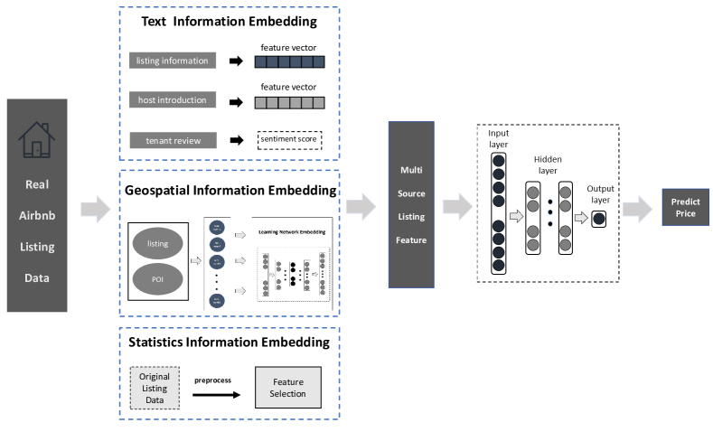
Figure 1: Framework Overview.

III Multi-Source Information Learning

In this section, we introduce the core architecture of our framework as follows: (1) statistic feature embedding; (2) text feature embedding; (3) spatial feature embedding.

III-A Statistics Feature Embedding

Each house’s statistic feature is represented by a 245- dimensional vector which describes the listing of a house, including listing_id, host_id, host_since, host_response_rate, host_is_superhost, host_has_profile_pic, host_identity_verified, bathrooms, bedrooms, latitude, longitude, accommodates, security_deposit, guests_included, verification, etc.

We use the Lasso CV to do the feature set selection. The loss function is defined as follows:

$$\text{ obj }=\frac{1}{2}\sum_{i=1}^{n}\left(\boldsymbol{y}_{\mathbf{i}}-\boldsymbol{w}^{T}\boldsymbol{x}_{\mathbf{i}}\right)^{2}+\alpha\sum_{j=1}^{m}\left|w_{\mathrm{i}}\right|$$ (1)

where $n$ is the number of houses, $m$ is the number of parameters, $\alpha$ is the regularization coefficient, $\alpha\sum_{j=1}^{m}\left|w_{\mathrm{i}}\right|$ is the L1 regularization term, $y_{i}$ is the rental price, $x_{i}$ is the statistical features of rental housing, $w$ is the coefficient matrix of rental housing features, $x_{i}=s_{i}$. Statistical feature matrix $\bf S$ =$\left(s_{1},s_{2},...,s_{n}\right)$. Lasso CV can compress the coefficients of unimportant features to 0, realizing the purpose of feature selection, and ultimately leaving the important statistical feature set that this paper wants.

III-B Text Feature Embedding

We extract three types of text data from the original data, there are listing description, host introduction and tenant review. Listing description mainly about introducing the location of the house, surrounding environment, indoor layout and housing regulations, etc. Host introduction mainly introduces the age, height, occupation, hobbies and personality of the host, and tenant review expresses the tenants’ feelings about housing rentals and the evaluation of the host’s attitudes. Since tenant review contain emotional value, we use two different methods to model text feature. We first use CBOW [14] model to embed the text feature of listing description, host introduction. We selects the Wikipedia Chinese thesaurus after preprocessing as the training corpus $W$, the objective function is defined as follows:

$$\mathcal{L}=\sum_{c\in W}\left\{\log\left[\sigma\left(x_{c}^{T}\theta^{c}\right)\right]+\sum_{u\in NEG(c)}\log\left[\sigma\left(-x_{c}^{T}\theta^{u}\right)\right]\right\}$$ (2)

Then the above objective function is optimized by using the random gradient rise method to obtain:

$$\mathcal{L}(c,u)=L^{c}(u)\log\left[\sigma\left(x_{c}^{T}\theta^{u}\right)\right]+\left[1-L^{c}(u)\right]\log\left[1-\sigma\left(x_{c}^{T}\theta^{u}\right)\right]$$ (3)

Then calculate the gradient of $\mathcal{L}(c,u)$ to obtain:

$$\boldsymbol{v}(\tilde{c}):=\boldsymbol{v}(\tilde{c})+\eta\sum_{u\in\{c\}\cup NEG(c)}\frac{\partial\mathcal{L}(c,u)}{\partial x_{c}}$$ (4)

In this paper, we set the dimension of the word vector as 100. $l$ and $h$ represent the embedding of listing description, host introduction, respectively.

$$l=\frac{1}{Z}\sum_{i=1}^{Z}v\left(\tilde{c}_{l}\right)$$ (5)

$$h=\frac{1}{z}\sum_{i=1}^{z}v\left(\tilde{c}_{h}\right)$$ (6)

Therefore, we get the text information feature matrix of the listing description and host introduction: $\bf L$ =$\left(l_{1},l_{2},...,l_{n}\right)$ and $\bf H$ =$\left(h_{1},h_{2},...,h_{n}\right)$.

For the tenant review embedding, since it contains strong emotional expression, in order to reflect whether the tenants’ evaluation of the house is positive or negative, we uses the naive Bayes method to generate the corresponding emotional score $r\in[0,1]$ for each house, where 0 represents the negative and 1 represents the positive. Specifically, the probability that a tenant review text belongs to the positive class can be expressed as:

$$P\left(pos\mid c_{1},\ldots c_{d}\right)=\frac{P\left(c_{1},\ldots c_{d}\mid pos\right)P(pos)}{P\left(c_{1},\ldots c_{d}\right)}$$ (7)

After simplifying the above formula, we can obtain:

$$P\left(pos\mid c_{1},\ldots c_{d}\right)=\frac{1}{1+\gamma}$$ (8)

In this work, a text represents a tenant’s review, and a tenant has many reviews, so the emotional score of a tenant can be expressed as:

$$r=\frac{1}{q}\sum_{i=1}^{q}P\left(\operatorname{pos}\mid c_{1},\ldots c_{d}\right)$$ (9)

where $q$ represents the number of reviews on a rental, $d$ represents the total number of words in a review, and $P\left(\operatorname{pos}\mid c_{1},\ldots c_{d}\right)$ represents the probability that the review belongs to the category of positive emotions. Therefore, the emotional score vector of tenant reviews can be expressed as $\bf R$ =$\left(r_{1},r_{2},...,r_{n}\right)$.

III-C Spatial Feature Embedding

We proposes a method to learn spatial embedding. First, POI is divided into 8 different types, and the rented houses and the surrounding different type POIs form a spatial network. Then learn the network embedding of these spatial graphs through SDNE model. This method can accurately capture the spatial features related to important POIs such as scenic spots and railway stations.

We uses Euclidean distance to calculate the weight $W$ between house and poi as follows:

$$W=R\cdot\arccos(\text{ dis })\cdot\pi/180$$ (10)

where $dis=\sin(Lat_{A})\sin(Lat_{B})\cos(Lon_{A}-Lon_{B})+\cos(Lat_{A})\cos(Lat_{B})$, the two types of nodes, A and B, represent the rental houses and POI respectively. $Lon_{A}$ and $Lon_{B}$ are their longitudes, $Lat_{A}$ and $Lat_{B}$ are their latitudes, and $R$ is the average radius of the earth, taking the value of 6371.004km.

In SDNE model, the encoder is from $x_{i}$ to $y_{i}^{(k)}$, the decoder is from $y_{i}^{(k)}$ to $\widehat{x}_{i}$, $y_{i}^{(k)}$ is the node embedding of $v_{i}$, in this paper,$y_{i}^{(k)}=p_{i}$. The formula of encoder is:

$$\boldsymbol{y}_{\boldsymbol{i}}^{(\boldsymbol{k})}=\sigma\left(\boldsymbol{W}^{(\boldsymbol{k})}\boldsymbol{y}_{\boldsymbol{i}}^{(\boldsymbol{k}-\mathbf{1})}+b^{(k)}\right)$$ (11)

Therefore, the spatial embedding can be expressed as $\bf P$ =$\left(p_{1},p_{2},...,p_{n}\right)$. After we get the statistic embedding, the text embedding and the spatial embedding. We combine the above features into a multi-source feature $M=(S,T,P)$, and use the fully connected neural network to predict the rental price. We take the multi-source feature matrix $\bf M$ =$\left(m_{1},m_{2},...,m_{n}\right)$ as the input of the neural network, then obtain as follows:

$$\boldsymbol{y}=w^{T}\boldsymbol{m}+b,\quad A=\sigma(\boldsymbol{y})$$ (12)

where $y$ is the actual rental price, $m$ is the multi-source feature, $w$ is the parameter matrix, and $b$ is the offset term. $A$ is the activation function, we uses ReLU function as the activation function. At last, the output layer uses a neuron to output and get the predicted price $\widehat{y}_{i}$.

IV Experiment

In this section, we first introduce two real dataset and evaluation metrics. Then, we design experiments to answer the following three questions:

• Q1. How is the performance of our proposed MSIE in the airbnb price prediction task?

• Q2. How do the feature combination affect the price prediction performance?

• Q3. What is the key influence on the airbnb price?

IV-A Dataset

We collect the dataset from an open online airbnb website. Table I shows the statistics of our two real airbnb datasets from two cities: Beijing and Shanghai after preprocess.

TABLE I: Statistics of the data

City	# Houses	# Reviews	Time Period
Beijing	10779	191876	01/2017-06/2019
Shanghai	8638	159069	01/2020-07/2021

Besides, we also collect the POI of the Beijing and Shanghai in Table II. We divide it into 8 categories, include, Education, Entertainment, Food, Beverage Shopping, Tourist, Transportation, Medical Service, and Public Service.

TABLE II: POI Categories

Number	POI Category Name	#Beijing	#Shanghai
1	Education	8711	2635
2	Entertainment	6501	2607
3	Food	5744	6301
4	Beverage Shopping	6601	5632
5	Tourist	6713	4176
6	Transportation	4322	1753
7	Medical Service	3660	2862
8	Public Service	5976	3699

IV-B Evaluation Metrics

We evaluate the model performances in terms of the following metrics.

(1) $\textbf{Mean Absolute Error}(\textbf{MAE})$ represents the average of the absolute value of the error between the predicted value and the true value.

$$\textbf{MAE}=\frac{1}{n}\sum_{i=1}^{n}\left|\hat{y}-y\right|$$ (13)

(2) $\textbf{Mean Squared Error}(\textbf{MSE})$ is a measure of the closeness of the predicted value relative to the actual value.

$$\textbf{MSE}=\frac{1}{n}\sum_{i=1}^{n}\left(\hat{y}-y\right)^{2}$$ (14)

(3) $\textbf{Root Mean Squared Error}(\textbf{RMSE})$ is defined as follows:

$$\textbf{RMSE}=\sqrt{\frac{1}{n}\sum_{i=1}^{n}\left(\hat{y}-y\right)^{2}}$$ (15)

where $\hat{y}$ is the predicted price from the regression and $y$ is the actual price. The lower the RMSE, the better the method.

(4) $\textbf{The coefficient of determination}(R^{2})$ convert the predicted results into accuracy, the results are between [0,1].

$$R^{2}=1-\frac{\sum_{i=1}^{n}\left(\hat{y}_{i}-y_{i}\right)^{2}}{\sum_{i=1}^{n}\left(\bar{y}_{l}-y_{i}\right)^{2}}$$ (16)

The higher the value of $R^{2}$ , the more accurate the estimation method.

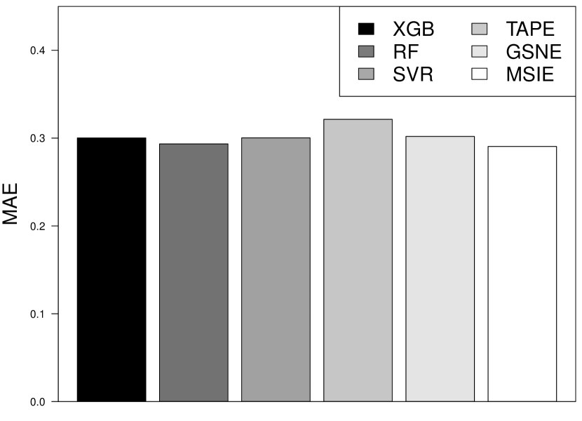
(a) MAE

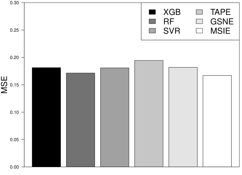
(b) MSE

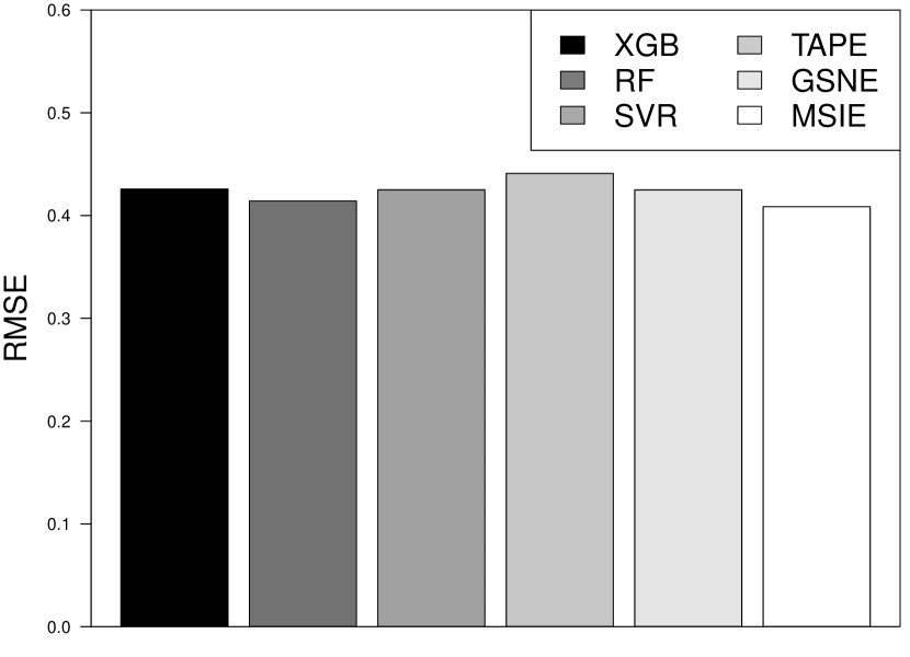
(c) RMSE

(d) $R^{2}$

Figure 2: Overall comparison on Beijing dataset.

(a) MAE

(b) MSE

(c) RMSE

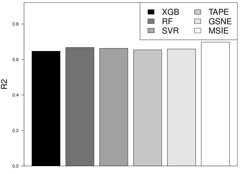
(d) $R^{2}$

Figure 3: Overall comparison on Shanghai dataset.

IV-C Baseline Algorithms

To prove the effectiveness of our model, we compare our method with the following algorithms.

(1)Extreme Gradient Boosting XGBOOST [15] is an improvement on the boosting algorithm based on Gradient Boosting Decision Tree to make it faster and more efficient.

(2)Random Forest RF [16] is an algorithm that integrates multiple trees through the idea of integrated learning. Its basic unit is the decision tree.

(3)Support Vector Regression SVR [17] is an algorithm that applies support vector machine to regression problems.

(4)TAPE TAPE [18] analyzed the relationship between the description of each rental and the price, and added the geographical factor component to recommend a reasonable price for each new rental of the landlord.

(5)GSNE GSNE [19] is a geospatial embedding framework, which can accurately capture the geospatial neighborhood relationship between houses and surrounding POIs. Essentially, it is to learn the low dimensional Gaussian embedding on the geospatial network node, and can be combined with the regression method, which has a certain effect on house price prediction.

Besides, our proposed model has three variants of the feature set combination: (1) MSIE-S, where the model utilizes the statistic feature; (2) MSIE-ST, where the model utilizes the statistic feature and text feature; (3) MSIE-STP, where the model utilizes the statistic feature, text feature and spatial feature. We evaluate these three variants with our model.

In the experiment, we split the dataset into two nonoverlapping sets: for all records, the earliest $80\%$ of records are the training set and the remaining $20\%$ are testing set. We implement the model by Pytorch and run the code on Windows10, Inter(R) Core(TM) i7-7700HQ @2.80GHZ and memory size 8G.

IV-D Overall Performances

We present the results for “MAE”, “MSE”, “RMSE” and “$R^{2}$”, compared with baseline algorithms. Figure 2 and Figure 3 show that our proposed method ”MSIE” outperform the baselines over both the Beijing and Shanghai dataset. The lower value of ”MAE”, ”MSE”, ”RMSE”, and the higher value of ”$R^{2}$”, means the performance better. In all cases, we observe an improvement with respect to baseline algorithms, especially on “MSE” and “$R^{2}$”. One interesting observation is that the traditional machine learning method(such as, ”XGB”, ”RF” and ”SVR”) performs better than ”TAPE”. We analysis the reason is that our algorithm feature engineering proposed in this paper is well done and has universality.

Besides, we uses the fully connected neural network constructed as the prediction model. In order to prevent over fitting, we sets 128 neurons in the input layer, uses 2 hidden layers and set Epoch=120, the size of Batch as 256. Figure 4 show the loss curves of neural network training on the two datasets respectively.

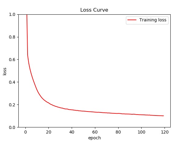
(a) Beijing

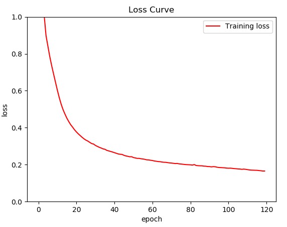
(b) Shanghai

Figure 4: The loss curve on two datasets.

IV-E Robustness Check

We evaluate the feature embedding contribution on modeling representations. To set the control group, we develop a variant of the proposed ”MSIE”, namely ”MSIE-S”, ”MSIE-ST”, ”MSIE-STP”. ”MSIE-S”, ”MSIE-ST”, ”MSIE-STP” takes the different combination of feature set as the input, while other component of remains the same. Table III and Table IV show the comparison results. We can observe that the performance of ”MSIE-STP” outperforms ”MSIE-S” and ”MSIE-ST” in terms of the four metrics over both two datasets. The results validate that the integration of text feature and spatial feature indeed enhances the modeling of price prediction.

TABLE III: The feature combination on Beijing dataset.

Feature set	MAE	MSE	RMSE	$R^{2}$
MSIE-S	0.3652	0.2341	0.4839	0.5545
MSIE-ST	0.2941	0.1688	0.4109	0.6786
MSIE-STP	0.2905	0.1669	0.4086	0.6824

TABLE IV: The feature combination on Shanghai dataset.

Feature set	MAE	MSE	RMSE	$R^{2}$
MSIE-S	0.4003	0.2852	0.5340	0.5824
MSIE-ST	0.3512	0.2371	0.4869	0.6527
MSIE-STP	0.3310	0.2065	0.4544	0.6977

IV-F Analysis of Key Influence

In order to analysis the key feature-influence of price, according to the previous studies, we use three feature selection method, include manual selection, P-value [20] and Lasso CV [21]. We use $R^{2}$ as an indicator to analyze, and the results are shown in Figure 5. The best result is to use Lasso CV to select features from the original data.

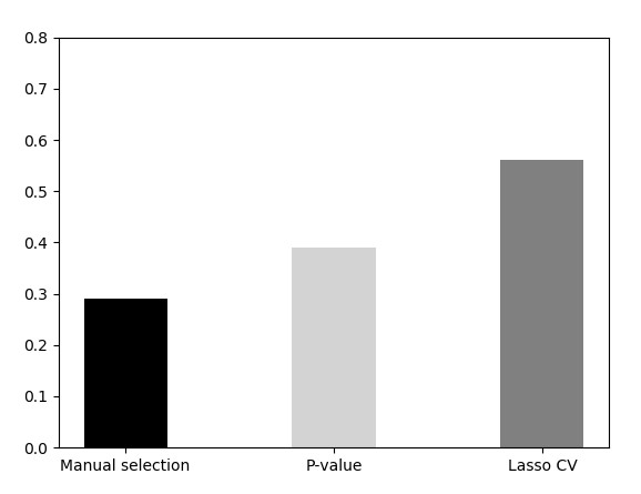
(a) Beijing

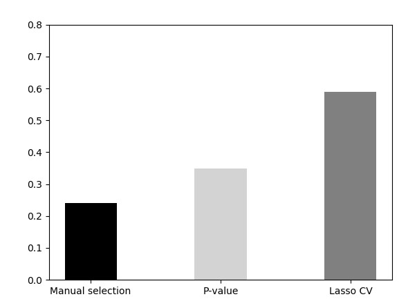
(b) Shanghai

Figure 5: The $R^{2}$ with different feature selection method.

Then, we selects 20 features with the highest correlation for rental price prediction according to P-value, and uses Lasso CV to select features to obtain statistical information as input for prediction. Figure 6 show the 10 features with the highest correlation with rental prices in the two datasets.

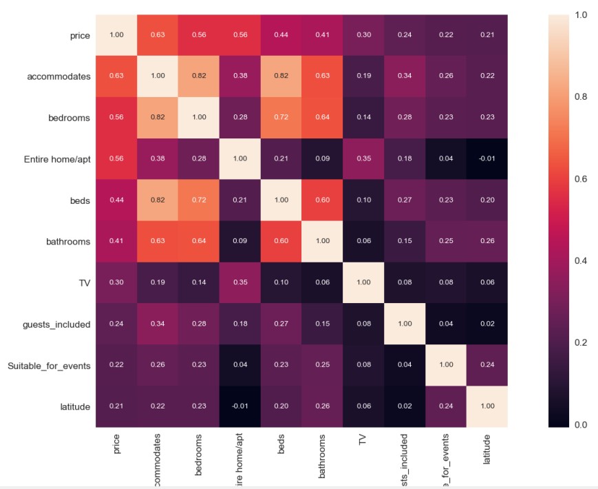
(a) Beijing

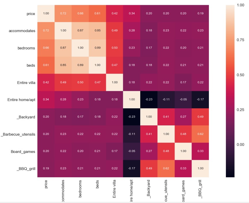
(b) Shanghai

Figure 6: The feature most relevant to price.

V Related work

In this work, we propose a model to predict the price of listings on Airbnb. Some studies used sentiment analysis to study the problem of Airbnb. Martinez R D et al. studied the relationship between Airbnb host’s listing description and occupancy rates by sentiment analysis [22]. Zhang et al. proposed a text analytics framework to study the relationship among self-description, trust perception and purchase behavior on Airbnb. They used text mining to extracted sentiment intensity and use regression method to identify the impact of linguistic and semantic features on trust perception [23]. Kalehbast P R et al. used sentiment analysis and machine learning to predict the price of listings on Airbnb [24].

Most researches have proposed many works to study the price by using the listing information. Wang et al. studied the relationship between a price and its determinants by various listing information (e.g., host identity verified, accommodates, wireless Internet, amenities and services, and free parking) [25]. P.Choudhary et al. analyzed Airbnb listings in San Francisco to better understand how different attributes (e.g., bedrooms, location, and listing type) can be used to accurately predict the price of a new listing, which is optimal in terms of the host’s profitability yet affordable to their guests [26]. Shen et al. analyzed the relationship between the description of each listing and its price, and proposed a text-based model to recommend a reasonable price for newly added listings [27]. Tang et al. labeled text information for nine handpicked classes, extracted image-related features, and finally used all features to predict a listing’s neighborhood and its price [28].

VI Conclusion

In this paper, we proposes a prediction model based on multi-source information embedding to study the Airbnb price problem. Specifically, in order to obtain the best feature set, we first selects the features of the house itself to obtain statistical information features. Secondly, the text information in this paper is divided into three categories, and the house description and landlord introduction are converted into feature matrix. The tenant reviews are then converted into sentiment scores about each house. Then, we uses different types of point-of-interest (POI) data and houses to form various spatial network graphs and learns their network embeddings to obtain spatial information features. Finally, we combines these three types of feature embeddings are combined into multi-resource housing features as input, and the neural network constructed in this paper is used for price prediction. The effectiveness of our model is demonstrated with two real data. For future work, we plan to combine some heuristic methods [29, 30] to further improve performance.

References

- [1] S. Rosen, “Hedonic Prices and Implicit Markets: Product Differentiation in Pure Competition,” Journal of Political Economy, vol. 82, no. 1, pp. 34–55, Jan.-Feb. 1974.
- [2] P. Morano and F. Tajani, “Bare ownership evaluation. hedonic price model vs. artificial neural network,” Int. J. Bus. Intell. Data Min., vol. 8, no. 4, pp. 340–362, 2013.
- [3] X. Xu, Z. Huang, J. Wu, Y. Fu, N. Luo, W. Chen, J. Wang, and M. Yin, “Finding the key influences on the house price by finite mixture model based on the real estate data in changchun,” in DASFAA, vol. 11448, 2019, pp. 378–382.
- [4] X. Xu, Y. Fu, J. Wu, Y. Wang, Z. Huang, Z. Fu, and M. Yin, “Adaptive weighted finite mixture model: Identifying the feature-influence of real estate,” Trans. Data Sci., vol. 1, no. 3, pp. 20:1–20:16, 2020.
- [5] Y. Fu, Y. Ge, Y. Zheng, Z. Yao, Y. Liu, H. Xiong, and J. Yuan, “Sparse real estate ranking with online user reviews and offline moving behaviors,” in ICDM, 2014, pp. 120–129.
- [6] Y. qing Li, T. Wang, and S. fei Zhao, “Application of svm based on rough set in real estate prices prediction,” in WiCOM, 2008, pp. 1–4.
- [7] P. R. Kalehbasti, L. Nikolenko, and H. Rezaei, “Airbnb price prediction using machine learning and sentiment analysis,” in Lecture Notes in Computer Science, 2021, pp. 173–184.
- [8] X. Chen, L. Wei, and J. Xu, “House price prediction using LSTM,” CoRR, vol. abs/1709.08432, 2017.
- [9] P. Wang, Y. Fu, J. Zhang, X. Li, and D. Lin, “Learning urban community structures: A collective embedding perspective with periodic spatial-temporal mobility graphs,” ACM Trans. Intell. Syst. Technol., vol. 9, no. 6, pp. 63:1–63:28, 2018.
- [10] P. Wang, Y. Fu, H. Xiong, and X. Li, “Adversarial substructured representation learning for mobile user profiling,” in SIGKDD. ACM, 2019, pp. 130–138.
- [11] P. Wang, K. Liu, L. Jiang, X. Li, and Y. Fu, “Incremental mobile user profiling: Reinforcement learning with spatial knowledge graph for modeling event streams,” in KDD, 2020.
- [12] P. Wang, Y. Fu, J. Zhang, P. Wang, Y. Zheng, and C. C. Aggarwal, “You are how you drive: Peer and temporal-aware representation learning for driving behavior analysis,” in SIGKDD, 2018, pp. 2457–2466.
- [13] D. Wang, P. Cui, and W. Zhu, “Structural deep network embedding,” in SIGKDD, 2016, pp. 1225–1234.
- [14] Q. Luo, W. Xu, and J. Guo, “A study on the CBOW model’s overfitting and stability,” in Web-KR@CIKM. ACM, 2014, pp. 9–12.
- [15] T. Chen and C. Guestrin, “Xgboost: A scalable tree boosting system,” in ACM, 2016.
- [16] L. Breiman, “Random forests,” Mach. Learn., vol. 45, no. 1, pp. 5–32, 2001.
- [17] M. Awad and R. Khanna, Support Vector Regression. Berkeley, CA: Apress, 2015, pp. 67–80.
- [18] L. Shen, Q. Liu, G. Chen, and S. Ji, “Text-based price recommendation system for online rental houses,” Big Data Min. Anal., vol. 3, no. 2, pp. 143–152, 2020.
- [19] S. S. S. Das, M. E. Ali, Y. Li, Y. Kang, and T. Sellis, “Boosting house price predictions using geo-spatial network embedding,” Data Min. Knowl. Discov., vol. 35, no. 6, pp. 2221–2250, 2021.
- [20] R. Feise, “Do multiple outcome measures require p-value adjustment?” BMC Med Res Methodol., vol. 2, no. 8, 2002.
- [21] H. Zou, “The adaptive lasso and its oracle properties,” Journal of the American Statistical Association, vol. 101, no. 476, pp. 1418–1429, 2006.
- [22] R. D. Martinez, A. Carrington, T. Kuo, L. Tarhuni, and N. Abdel-Motaal, “The impact of an airbnb host’s listing description ’sentiment’ and length on occupancy rates,” 2017.
- [23] L. Zhang, Q. Yan, and L. Zhang, “A text analytics framework for understanding the relationships among host self-description, trust perception and purchase behavior on airbnb,” Decision Support Systems, vol. 133, p. 113288, 2020.
- [24] P. R. Kalehbasti, L. Nikolenko, and H. Rezaei, “Airbnb price prediction using machine learning and sentiment analysis,” 2019.
- [25] D. Wang and J. L. Nicolau, “Price determinants of sharing economy based accommodation rental: A study of listings from 33 cities on airbnb.com,” International Journal of Hospitality Management, vol. 62, pp. 120–131, 2017.
- [26] P. Chou D Hary, A. Jain, and R. Baijal, “Unravelling airbnb predicting price for new listing,” Papers, 2018.
- [27] L. Shen, Q. Liu, G. Chen, and S. Ji, “Text-based price recommendation system for online rental houses,” Big Data Mining and Analytics, vol. 3, no. 2, pp. 143–152, 2020.
- [28] E. Tang and K. Sangani, “Neighborhood and price prediction for san francisco airbnb listings,” 2015.
- [29] Y. Wang, S. Cai, J. Chen, and M. Yin, “Sccwalk: An efficient local search algorithm and its improvements for maximum weight clique problem,” Artif. Intell., vol. 280, p. 103230, 2020.
- [30] S. Pan, Y. Ma, Y. Wang, Z. Zhou, J. Ji, M. Yin, and S. Hu, “An improved master-apprentice evolutionary algorithm for minimum independent dominating set problem,” Frontiers of Computer Science, vol. 17, no. 4, pp. 1–14, 2023.