Consensus-based Distributed Intentional Controlled Islanding of Power Grids

Abstract

The problem of partitioning a power grid into a set of islands can be a solution to restore power dispatchment in sections of a grid affected by an extreme failure. Current solutions to this problem usually involve finding the partition of the grid into islands that minimizes the sum of their absolute power imbalances. This combinatorial problem is often solved through heuristic offline methods. In this paper, we propose instead a distributed online algorithm through which nodes can migrate among islands, self-organizing the network into a suitable partition. We prove that, under a set of appropriate assumptions, the proposed solution yields a partition whose absolute power imbalance falls within a given bound of the optimal solution. We validate our analytical results by testing our partitioning strategy on the IEEE 118 and 300 benchmark problems.

I Introduction

The penetration of renewable and distributed generation, e.g., [1, 2, 3], and the possible occurrence of cascading failures [4] have made the problem of devising control strategies to govern the operation of power grids of crucial concern. Examples of problems of interest include those reported in [5, 6, 7], [8, 9] and [10, 11, 12].

When the control architecture fails to guarantee reliable operation of the transmission grid, last resort strategies have been devised so as to ensure power dispatchment across at least some of its sections. Intentional Controlled Islanding (ICI) strategies address this issue [13, 14, 15, 16, 17] by identifying sections of the grid (or islands) that can isolate and operate independently from the rest of the network. Recently, intentional islanding has also been proposed in the framework of distribution networks, see [18] and references therein, as the presence of storage devices and renewable energy generation allows these grids to be partitioned into networks of microgrids, e.g., [19, 20, 21].

The problem of partitioning a grid into a set of islands is usually mathematized as a combinatorial problem—see for example [19, 22, 23, 24]—and sometimes it is recast as a graph optimization problem [17, 15, 16]. Often, solving these problems numerically is cumbersome or inefficient, so that heuristic strategies are frequently used to seek a suboptimal solution, while meeting the required computational time that allows the network to stabilize after a contingency [13, 25, 26, 27].

In this paper, we propose a different distributed approach to solve the ICI problem, where network nodes can migrate from an island to another so as to self-organise into a partition minimizing the power imbalance between different islands and avoiding large amounts of load shedding. Specifically, starting from some initial partition of the grid, we endow the nodes with the ability of locally estimating the power imbalance of their island and of those neighboring it, so as to decide whether to migrate or not to a different island from their own.

The estimation strategy is completely distributed and decentralized and relies on nodes running a virtual consensus dynamics parameterized so that the consensus equilibrium the nodes reach is proportional to the power imbalance of the island of interest. Under suitable assumptions, we analytically show that our migration strategy generates a sequence of partitions that converge in finite time to a configuration whose average absolute power imbalance falls within a certain bound of the minimal one. We validate our strategy by partitioning the IEEE 118 and IEEE 300 test systems, comparing the viable partitions we obtain to others suggested in previous papers in the Literature.

II Preliminaries and problem statement

Notation

Given a set $\mathcal{Q}$, we denote by $\left\lvert\mathcal{Q}\right\rvert$ its cardinality; $\mathbf{1}$ is the column vector of ones, with appropriate dimension.

Power grid

We model a power grid as an undirected connected graph $\mathcal{G}=(\mathcal{V},\mathcal{E})$, where $\mathcal{V}$ is the set of $n\in\mathbb{N}_{>0}$ grid nodes (loads or generators) and $\mathcal{E}$ is the set of edges representing transmission lines interconnecting them. Without loss of generality, the $n_{\mathrm{g}}\in\mathbb{N}_{>0}$ generators are labeled as nodes $1,\dots,n_{\mathrm{g}}$, while the $n_{\mathrm{l}}\in\mathbb{N}_{>0}$ loads as nodes $n_{\mathrm{g}}+1,\dots,n$. We let $p_{i}\in\mathbb{R}$ be the active power generated or consumed at node $i$; $p_{i}>0$ if $i$ is a generator, while $p_{i}\leq 0$ if $i$ is a load. We let $A$ be the (symmetric) adjacency matrix associated to the graph $\mathcal{G}$; its $(i,j)$-th element $a_{ij}$ being $1$ if $\{i,j\}\in\mathcal{E}$ or $0$ otherwise.

Islands and neighbours

We define an island as a connected subgraph $\mathcal{M}_{l}=(\mathcal{V}_{l},\mathcal{E}_{l})$ of $\mathcal{G}$, where $\mathcal{V}_{l}\subseteq\mathcal{V}$ and $\mathcal{E}_{l}=\left(\mathcal{V}_{l}\times\mathcal{V}_{l}\right)\cap\mathcal{E}$. Given a set of nodes $\mathcal{V}_{l}$, we denote by $\mathcal{N}(\mathcal{V}_{l})$ the set of neighbours of the nodes in $\mathcal{V}_{l}$, i.e., $\mathcal{N}(\mathcal{V}_{l})\coloneqq\{i\in\mathcal{V}\setminus\mathcal{V}_{l}\mid\exists j\in\mathcal{V}_{l}:\{i,j\}\in\mathcal{E}\}$. We say that island $\mathcal{M}_{m}$ is a neighbor of island $\mathcal{M}_{l}$ if and only if $\mathcal{N}(\mathcal{V}_{m})\cap\mathcal{V}_{l}\neq\varnothing$. Moreover, we denote by $\mathcal{N}_{i}$ the set of neighbours of node $i$.

Grid partitions

We say that the grid is partitioned into $n_{\mu}\in\mathbb{N}_{>0}$ islands, described by the subgraphs $\mathcal{M}_{l},\dots,\mathcal{M}_{n_{\mu}}$, with corresponding node sets $\mathcal{V}_{1},\dots,\mathcal{V}_{n_{\mu}}$, if $\Pi=\{\mathcal{V}_{1},\dots,\mathcal{V}_{n_{\mu}}\}$ is a partition of $\mathcal{V}$. Additionally, a node, say $i$, in an island, say $\mathcal{M}_{l}$, is a boundary node if $\mathcal{N}_{i}\cap(\mathcal{V}\setminus\mathcal{V}_{l})\neq\varnothing$. Furthermore, we define the condensed graph $\mathcal{G}^{\Pi}=(\mathcal{V}^{\Pi},\mathcal{E}^{\Pi})$ induced by the partition $\Pi$, where node $l$ in $\mathcal{V}^{\Pi}$ is associated to $\mathcal{V}_{l}$ in $\Pi$, and an edge $\{l,m\}$ exists in $\mathcal{E}^{\Pi}$ if and only if $\mathcal{V}_{l}\cap\mathcal{N}(\mathcal{V}_{m})\neq\varnothing$.

Power imbalance

The power imbalance of an island $\mathcal{M}_{l}$ is

$$P_{l}\coloneqq\sum_{i\in\mathcal{V}_{l}}p_{i};$$ (1)

the overall grid’s power imbalance is

$$P_{\text{tot}}\coloneqq\sum_{i=1}^{n}p_{i}=\sum_{l=1}^{n_{\mu}}P_{l}.$$ (2)

The power imbalance in (1) is associated to the synchronous frequency deviation of the island from its nominal value, which in turn is related to the frequency’s stability [28, 9]. Indeed, if the generated power exceeds loads’ demand, the frequency increases, and vice-versa. Excessively large variations in the operating frequency with respect to the nominal one can cause faults.

Control problem

The problem we study is to find a partition of the power grid $\mathcal{G}$ into $n_{\mu}\geq 2$ microgrids so as to minimize the average absolute power imbalance, defined as

$$J\coloneqq\frac{1}{n_{\mu}}\sum_{l=1}^{n_{\mu}}|P_{l}|.$$ (3)

Note that, as $\sum_{l=1}^{n_{\mu}}|P_{l}|\geq\left|\sum_{l=1}^{n_{\mu}}P_{l}\right|=|P_{\text{tot}}|$, then

$$J\geq J^{*}\coloneqq\left|\frac{P_{\text{tot}}}{n_{\mu}}\right|.$$ (4)

The cost function in (3) has been used in previous work in the literature on grid partitioning, e.g. [19, 25, 13], as an indicator of the ability of a power system to satisfy the loads’ demand, which is also known as adequacy [29].

III A consensus based partitioning strategy

We propose a strategy that, given an initial partition $\Pi(0)$ of the power grid into $n_{\mu}$ islands, uses a consensus algorithm to let the nodes self-organise into a new partition that minimizes $J$, as defined in (3). In particular, at each step $k$ of the algorithm, one node can migrate between islands. We denote by $\Pi(k)$ the partition after $k$ migrations have occurred; $\mathcal{M}_{l}(k)=(\mathcal{V}_{l}(k),\mathcal{E}_{l}(k))$, $l\in\{1,\dots,n_{\mu}\}$ being the corresponding islands, $P_{l}(k)$, $l\in\{1,\dots,n_{\mu}\}$ their power imbalances, and $J(k)$ the corresponding value of the cost function.

Our strategy is based on two fundamental ingredients:

1. a distributed dynamic estimator based on average consensus dynamics that nodes can use to estimate the power imbalance in their island and in those of their neighbors;

2. a migration condition according to which a boundary node can decide whether to migrate from its island to a neighboring one.

Next, we describe the two elements above.

III-A Distributed power imbalance estimation

At any step $k$, each node, say $i$, can obtain an estimate of the power imbalance, say $P_{l}(k)$, of the island it belongs to or of an island neighboring it, say $\mathcal{M}_{l}(k)=(\mathcal{V}_{l}(k),\mathcal{E}_{l}(k))$, by running a consensus based estimation strategy.

Specifically, let us define the auxiliary graph $\widehat{\mathcal{M}}_{l}(k)\coloneqq(\widehat{\mathcal{V}}_{l}(k),\widehat{\mathcal{E}}_{l}(k))$ with

$$\widehat{\mathcal{V}}_{l}(k)\coloneqq\begin{dcases}\mathcal{V}_{l}(k)\setminus i,&\text{if }i\in{\mathcal{V}}_{l}(k),\\ \mathcal{V}_{l}(k)\cup i,&\text{if }i\notin{\mathcal{V}}_{l}(k),\end{dcases}$$ (5)

and $\widehat{\mathcal{E}}_{l}(k)\coloneqq(\widehat{\mathcal{V}}_{l}(k)\times\widehat{\mathcal{V}}_{l}(k))\cap\mathcal{E}$. To estimate $P_{l}(k)$, node $i$ must trigger the distributed solution of the two virtual continuous-time consensus dynamics given by

$$\dot{x}_{h}(t) =p_{h}+\sum_{\{j,h\}\in\mathcal{E}_{l}(k)}(x_{j}(t)-x_{h}(t)),\quad\forall{h}\in\mathcal{V}_{l}(k),$$ (6a)

$$\dot{\widehat{x}}_{h}(t) =p_{h}+\sum_{\{j,h\}\in\widehat{\mathcal{E}}_{l}(k)}(\widehat{x}_{j}(t)-\widehat{x}_{h}(t)),\quad\forall h\in\widehat{\mathcal{V}}_{l}(k),$$ (6b)

starting from null initial conditions. Here, $x_{h}(t)$ and $\widehat{x}_{h}(t)$ are the virtual states associated to each node $h\in\mathcal{V}_{l}(k)$ and $h\in\widehat{\mathcal{V}}_{l}(k)$, respectively.

Remark 1.

To run the consensus dynamics (6) in a distributed manner, we assume the virtual states $x_{h}$ and $\widehat{x}_{h}$ are broadcast to all neighboring nodes $\mathcal{N}_{h}\cap\mathcal{V}_{l}(k)$.

Now, dynamics (6a) can be recast in matrix form as

$$\dot{\boldsymbol{x}}(t)=\mathbf{p}-L\boldsymbol{x}(t),$$ (7)

where $\boldsymbol{x}$ is the stack vector of the virtual states $x_{h}$, $\mathbf{p}$ is the stack vector of the power values $p_{h}$, and $L$ is the (symmetric) Laplacian matrix associated to $\mathcal{M}_{l}(k)$. Let us recall that $\mathbf{1}^{\mathsf{T}}$ is an eigenvector of the symmetric Laplacian $L$, with $0$ as an associated eigenvalue. To obtain the asymptotic behaviour of (7), we premultiply (7) by $\mathbf{1}^{\mathsf{T}}$, obtaining, for all time $t$,

$$\mathbf{1}^{\mathsf{T}}\dot{\boldsymbol{x}}(t)=\mathbf{1}^{\mathsf{T}}\mathbf{p}=P_{l}(k).$$ (8)

Moreover, differentiating (7), we obtain the dynamical system $\ddot{\boldsymbol{x}}(t)=-L\dot{\boldsymbol{x}}(t)$, whose dynamics, determined by the spectral properties of $L$, are such that

$$\lim_{t\rightarrow\infty}\dot{\boldsymbol{x}}(t)\in\mathrm{span}(\mathbf{1}).$$ (9)

Altogether, (8) and (9) imply that $\lim_{t\rightarrow\infty}\dot{\boldsymbol{x}}(t)=\mathbf{1}\omega_{l}$, where

$$\omega_{l}\coloneqq\frac{P_{l}(k)}{|\mathcal{V}_{l}(k)|},$$ (10)

Similarly, from (6b), we obtain that $\lim_{t\rightarrow\infty}\dot{\widehat{\boldsymbol{x}}}(t)=\mathbf{1}\widehat{\omega}_{l}$, with

$$\widehat{\omega}_{l}\coloneqq\frac{1}{|\widehat{\mathcal{V}}_{l}(k)|}\sum_{j\in\widehat{\mathcal{V}}_{l}(k)}p_{j}.$$ (11)

Exploting (5), (11) can be recast as

$$\widehat{\omega}_{l}=\begin{dcases}\tfrac{1}{|\mathcal{V}_{l}(k)|-1}\left(P_{l}(k)-p_{i}\right),&\text{if }i\in\mathcal{V}_{l}(k),\\ \tfrac{1}{|\mathcal{V}_{l}(k)|+1}\left(P_{l}(k)+p_{i}\right),&\text{if }i\not\in\mathcal{V}_{l}(k).\end{dcases}$$ (12)

Then, (10) and (12) can be solved together for the unknowns $P_{l}(k)$ and $|\mathcal{V}_{l}(k)|$, obtaining

$$P_{l}(k)=a_{l}\omega_{l}\frac{p_{i}-\widehat{\omega}_{l}}{\widehat{\omega}_{l}-\omega_{l}},$$ (13a)

$$|\mathcal{V}_{l}(k)|=a_{l}\frac{p_{i}-\widehat{\omega}_{l}}{\widehat{\omega}_{l}-\omega_{l}},$$ (13b)

with

$$a_{l}=\begin{dcases}-1,&\text{if }i\in\mathcal{V}_{l}(k),\\ 1,&\text{if }i\not\in\mathcal{V}_{l}(k).\end{dcases}$$

From (13a), to estimate $P_{l}(k)$, node $i$ needs to compute $\omega_{l}$ and $\widehat{\omega}_{l}$. To do so in a distributed fashion, node $i$ starts the distributed computation of the consensus dynamics (6a) and (6b) by broadcasting its virtual states $x_{i}$ and $\widehat{x}_{i}$ to the nodes in ${\mathcal{N}}_{i}\cap\mathcal{V}_{l}(k)$. In turn, each of these starts sharing its virtual state with its neighbors (within $\mathcal{V}_{l}(k)$), until all nodes in $\mathcal{V}_{l}(k)$ join the distributed simulation. Note that the aforementioned procedure can be conducted through one-hop communication if each node $h$ has knowledge of the index $l\in\{1,...,n_{\mu}\}$ of the island it belongs to, and of its consumed or generated power $p_{h}$. Obviously, in a practical implementation, the grid nodes should be equipped with sufficient computational and communication capabilities to run the virtual consensus dynamics on a timescale that is compatible with the grid requirements.

In what follows, we will show how the network nodes can exploit this estimation process to self-organise into a partition of the power network whose power imbalance (3) is rendered minimal.

Figure 1: (a) Initial partition of the power network, with dashed lines representing the communication links among nodes; the topology being equal to that of the power network itself. (b) Boundary node 3 triggers the distributed simulation of the virtual consensus dynamics in (6) for both islands $\mathcal{M}_{1}$ and $\mathcal{M}_{2}$. (c) The migration rule (14a) is used to decide whether to migrate from island $\mathcal{M}_{1}$ to $\mathcal{M}_{2}$ and (d) a new partition is eventually generated.

III-B Migration Condition

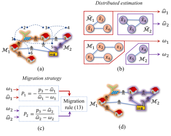
A boundary node (see § II), say $i$, in island $\mathcal{M}_{m}(k)$, can decide whether to migrate to a neighboring island $\mathcal{M}_{l}(k)$ (see Figure 1) by assessing the power imbalances $P_{l}(k)$ and $P_{m}(k)$ (computed through our estimation strategy in § III-A).

Specifically, at step $k$, node $i$ will migrate from $\mathcal{M}_{m}(k)$ to $\mathcal{M}_{l}(k)$ if and only if

$$\min(P_{l}(k),P_{m}(k))<\min(P_{l}(k+1),P_{m}(k+1)),$$ (14a)

$$\mathcal{M}_{m}(k+1)\ \mathrm{is\ connected},$$ (14b)

with

$${P}_{l}(k+1) ={P}_{l}(k)+p_{i},$$ (15a)

$${P}_{m}(k+1) ={P}_{m}(k)-p_{i},$$ (15b)

$$\mathcal{V}_{l}(k+1) =\mathcal{V}_{l}(k)\cup i,$$ (15c)

$$\mathcal{V}_{m}(k+1) =\mathcal{V}_{m}(k)\setminus\{i\}.$$ (15d)

Remark 2.

Condition (14b) concerning connectivity can be ensured using the estimation strategy in § III-A. Indeed, given an island $\mathcal{M}_{l}(k)$, if there exists a node $i\in\mathcal{V}_{l}(k)$ such that $\mathcal{M}_{l}(k)\setminus\{i\}$ is not connected, the virtual derivatives $\dot{\widehat{x}}_{h}$ of its neighbors in $\widehat{\mathcal{M}}_{l}$ (see (6b)) will in general converge to different values, thus providing a warning signal.

III-C Migration Algorithm

According to our decentralised partitioning strategy, starting from some initial partition at step $k=0$, each boundary node must trigger the distributed estimation of the power imbalance of the island it belongs to and of its neighboring islands by running the virtual consensus dynamics (6). Then, depending on these power imbalances, exploiting the migration condition (14a), the boundary nodes will decide whether to migrate or not to neighboring islands.

For the sake of clarity, we illustrate the process by referring to the exemplary situation depicted in Figure 1, where a grid with $n=6$ nodes is initially partitioned in $n_{\mu}=2$ islands, $\mathcal{M}_{1}(0)$ and $\mathcal{M}_{2}(0)$ (Figure 1(a)). Then, each boundary node, as for instance node $3\in\mathcal{V}_{1}(0)$, must decide whether to migrate to the other island ($\mathcal{M}_{2}$) or not. To this aim, node 3 triggers the distributed estimation of the power imbalances $P_{1}(0)$ and $P_{2}(0)$ in both the islands $\mathcal{M}_{1}(0)$ and $\mathcal{M}_{2}(0)$ (see Figure 1(b)), by running two virtual consensus processes of the form (6) involving all nodes belonging to each of the islands. Once a steady state in the distributed simulation of (6) has been reached, node 3 uses the pairs $(\omega_{1},\hat{\omega}_{1})$ and $(\omega_{2},\hat{\omega}_{2})$ to estimate $P_{1}(0)$ and $P_{2}(0)$, which it then uses to evaluate the migration condition (14a) (Figure 1(c)) to assess whether to migrate from $\mathcal{M}_{1}$ to $\mathcal{M}_{2}$. Once this decision is taken, a new partition is generated (Figure 1(d)).

In general, our strategy prescribes that the grid nodes get involved in all the (possibly multiple) distributed consensus processes invoked according to (6) by the boundary nodes of their island or of neighboring ones so as to allow the estimation of the power imbalances of interest. Hence, at any time, each node will have a number of virtual states corresponding to the number of estimation processes it is asked to contribute to. These steps are summarized in Algorithm 1. Additionally, as soon as a node becomes a boundary node (see § II), it must trigger additional virtual dynamics to decide whether to migrate or not from its island to a neighboring one. This additional procedure is summarized in Algorithm 2.

The following Lemma and Theorem, whose proofs are given in Section V, state that the migration process governed by rule (14a) generates a finite sequence $\{\Pi(k)\}_{k\in\{0,\dots,K\}}$ of $K\in\mathbb{N}$ migration steps, and give a bound on the difference between the cost $J(K)$ of the final partition and the optimal cost $J^{*}$ computed in (4).

Lemma 1.

If

$$|P_{l}(k)-P_{m}(k)|\leq\bar{p}\quad\forall l,m:\mathcal{N}(\mathcal{V}_{m}(k))\cap\mathcal{V}_{l}(k)\neq\varnothing,$$ (16)

where $\bar{p}\coloneqq\max_{i\in\mathcal{V}}|p_{i}|$, then

$$J(k)-J^{*}\leq\frac{2}{n_{\mu}}\left(\sum_{l=l^{*}+1}^{n_{\mu}}p^{*}+\bar{p}\left(l-\frac{n_{\mu}+1}{2}\right)\right)-(p^{*}+|p^{*}|),$$ (17)

with

$$l^{*}=\left\lceil-\frac{p^{*}}{\bar{p}}+\frac{n_{\mu}+1}{2}\right\rceil,$$ (18)

and $p^{*}\coloneqq P_{\text{tot}}/n_{\mu}$.

Theorem III.1.

Assume that at each step $k$ there exist a node $i$ and islands $\mathcal{M}_{l}(k)$ and $\mathcal{M}_{m}(k)$ (that is a triplet $(l,m,i)$) such that

$$\left\{\begin{array}[]{c}i\in\left\{\mathcal{V}_{m}(k)\cap\mathcal{N}(\mathcal{V}_{l}(k))\right\}\\ \wedge\\ \mathcal{M}_{m}(k)\setminus i\text{ is connected }\end{array}\right.$$ (19a)

and

$$\left\{\begin{array}[]{c}P_{l}(k)>P_{m}(k)\;\wedge\;p_{i}<0\\ \lor\\ P_{l}(k)<P_{m}(k)\;\wedge\;p_{i}>0.\end{array}\right.$$ (19b)

Then, the sequence $\Pi(k)$ obtained under the migration rule (14a) is finite and converges in $K<+\infty$ steps to a partition $\Pi(K)$ such that $J(k)$ fulfills (17) at $k=K$.

In the following section, we validate the strategy numerically. A formal proof of convergence is provided later in Section V.

1 Broadcast all virtual states to neighboring nodes

2Obtain virtual states from neighboring nodes

Integrate (6) for all simulations where $h$ is involved

Algorithm 1 Default routine for any node $h$.

1 Communicate with the nodes in $\mathcal{N}_{h}\cap\mathcal{V}_{m}$ to trigger a distributed simulation of (6)

2for  $l:\mathcal{N}_{h}\cap\mathcal{V}_{l}\neq\varnothing$ do

3       Communicate with the nodes in $\mathcal{N}_{h}\cap\mathcal{V}_{l}$ to trigger a distributed simulation of (6)

4      Wait for steady state in such simulations

5      Estimate $P_{m}$ and $P_{l},\ \forall l:\mathcal{N}_{h}\cap\mathcal{V}_{l}\neq\varnothing$ using (13)

6      Decide whether to migrate from $\mathcal{M}_{m}$ to $\mathcal{M}_{l}$ via (14a)

7

Algorithm 2 Additional steps for a boundary node $h\in\mathcal{V}_{m}$.

IV Numerical Validation

We demonstrate the effectiveness of our algorithm by deploying it to partition the IEEE 118 and 300 testbed cases [30]. The nodal power values $p_{i}$ are computed by solving an Optimal Power Flow (OPF) problem, leveraging Matpower 6.0 [31]. As the test cases include nodes with null nodal power $p_{i}=0$, we allow for these nodes to migrate from their island, say $\mathcal{M}_{m}(k)$, to a neighboring island, say $\mathcal{M}_{l}(k)$, as long as (i) their migration does not render $\mathcal{M}_{m}(k)$ disconnected and (ii) $P_{l}(k)\neq P_{l}(k^{\prime}),\forall k^{\prime}<k:i\in\mathcal{V}_{l}(k^{\prime})$.

To apply our partitioning strategy (Algorithms 1, 2), we need some initial partitions $\Pi(0)$, and to test our algorithm under different conditions, we considered multiple possible $\Pi(0)$. In some cases, we took as $\Pi(0)$ some selected partitions from [26, 32, 13]. In other cases, we used what we call the SSRP+BFS approach to generete $\Pi(0)$. Namely, we first employ the Search Space Reduction Procedure [26], which generates a spanning tree connecting groups of coherent generators (these are taken from [26]). Then, the remaining nodes are aggregated to the tree using the Breadth-First Search algorithm [33].

Remark 3.

Throughout our numerical analysis, whenever a node, say $i\in\mathcal{V}_{m}(k)$, can choose to migrate to more than one island, it will select the one maximizing the difference

$$\Delta P_{l}=\min\{P_{l}(k)+P_{i},P_{m}(k)-P_{i}\}-\min\{P_{l}(k),P_{m}(k)\}.$$

This choice ensures that the average absolute power imbalance is improved the most after the migration.

Case	$n_{\mu}$	$K$	Cut-set at $\Pi(0)$	$\Pi(0)$	Cut-set at $\Pi(K)$	$J(0)$	$J(K)$	$J^{*}$	$P_{l}(0)$	$P_{l}(K)$	Bound (17)
IEEE 118	2	10	$\begin{array}[]{c}\{24\text{-}70,34\text{-}43,\\ 37\text{-}40,38\text{-}65,\\ 39\text{-}40,71\text{-}72\}\end{array}$	SSRP+BFS	$\begin{array}[]{c}\{15\text{-}19,18\text{-}19,\\ 19\text{-}34,23\text{-}25,\\ 23\text{-}32,30\text{-}38,\\ 37\text{-}38,37\text{-}39,\\ 37\text{-}40,43\text{-}44\}\end{array}$	$120.5$	$58.25$	$58.25$	$\begin{array}[]{c}\{-74.26,\\ 190.75\}\end{array}$	$\begin{array}[]{c}\{53.74,\\ 62.75\}\end{array}$	213.14
IEEE 118	2	9	$\begin{array}[]{c}\{1\text{-}2,3\text{-}12,\\ 5\text{-}8,6\text{-}7,\\ 11\text{-}12,15\text{-}17,\\ 15\text{-}19,24\text{-}70,\\ 30\text{-}38,34\text{-}36,\\ 44\text{-}45,70\text{-}71\}\end{array}$	[13]	$\begin{array}[]{c}\{4\text{-}5,5\text{-}11,\\ 11\text{-}12,15\text{-}17,\\ 15\text{-}19,30\text{-}38,\\ 34\text{-}37,35\text{-}37,\\ 43\text{-}44,69\text{-}70,\\ 70\text{-}75,74\text{-}75\}\end{array}$	$265.5$	$58.25$	$58.25$	$\begin{array}[]{c}\{-258.25,\\ 374.74\}\end{array}$	$\begin{array}[]{c}\{65.75,\\ 50.74\}\end{array}$	213.14
IEEE 118	3	7	$\begin{array}[]{c}\{24\text{-}70,34\text{-}43,\\ 37\text{-}40,38\text{-}65,\\ 39\text{-}40,68\text{-}81,\\ 69\text{-}77,71\text{-}72,\\ 75\text{-}77,76\text{-}118\}\end{array}$	SSRP+BFS	$\begin{array}[]{c}\{19\text{-}34,21\text{-}22,\\ 23\text{-}25,23\text{-}32,\\ 30\text{-}38,34\text{-}36,\\ 34\text{-}37,37\text{-}38,\\ 37\text{-}39,37\text{-}40,\\ 68\text{-}81,69\text{-}77\\ 75\text{-}77,76\text{-}118\}\end{array}$	$80.34$	$38.83$	$38.83$	$\begin{array}[]{c}\{-74.26,\\ 1.98,\\ 188.77\}\end{array}$	$\begin{array}[]{c}\{53.74,\\ 1.98,\\ 60.77\}\end{array}$	335.97
IEEE 118	3	8	$\begin{array}[]{c}\{24\text{-}70,24\text{-}72,\\ 38\text{-}65,40\text{-}42,\\ 41\text{-}42,44\text{-}45,\\ 69\text{-}77,75\text{-}77,\\ 81\text{-}80,118\text{-}76\}\end{array}$	[26]	$\begin{array}[]{c}\{24\text{-}70,42\text{-}49,\\ 44\text{-}45,61\text{-}64,\\ 63\text{-}64,65\text{-}66,\\ 65\text{-}68,69\text{-}77,\\ 71\text{-}72,75\text{-}77,\\ 76\text{-}118,80\text{-}81\}\end{array}$	147	38.83	38.83	$\begin{array}[]{c}\{-199.26\\ 313.77\\ 1.98\}\end{array}$	$\begin{array}[]{c}\{83.66,\\ 30.86,\\ 1.98\}\end{array}$	335.97

TABLE I: Results after applying Algorithms 1 and 2 to the IEEE 118 test case, considering different initial partitions $\Pi(0)$. Power values are reported in MW. Note that bound (17) is computed for $k=K$.

IV-A IEEE 118 bus system

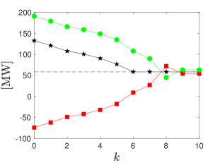
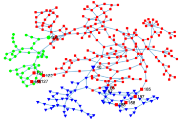
We used our Algorithm 1-2 to partition the IEEE 118 test system in $n_{\mu}=2$ and $n_{\mu}=3$ islands, considering only $n_{\mathrm{g}}=19$ generators (excluding the reactive compensators). We assume that the migration process is triggered by a three phase solid ground fault at bus 15 forcing line 14-15 to disconnect. With $n_{\mu}=2$, we considered as initial partition $\Pi(0)$ the one generated by SSRP+BFS and the final partition reported in [13]; with $n_{\mu}=3$, we considered as $\Pi(0)$ the partition generated by SSRP+BFS and the final one reported in [26]. All relevant information and the results are reported in Table I.

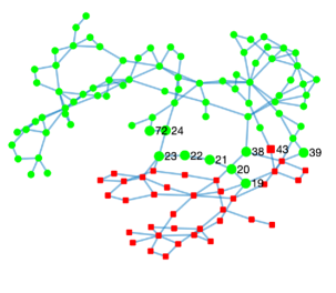
We observe that the proposed algorithm is indeed capable of converging in all cases towards partitions that minimize $J$, as $J(K)=J^{*}$. As a representative example, we depict in Figure 2 the case that $n_{\mu}=2$ and $\Pi(0)$ is generated by SSPR+BFS; namely, Figure 2(a) portrays the power imbalances $P_{1}(k)$ and $P_{2}(k)$ at the various steps, while the final partition $\Pi(K)$ is reported in Figure 2(b). Note that from the OPF results we have $\max_{i}|p_{i}|=542.78$ MW and $J^{*}=58.25$ MW and thus the bound given in Theorem III.1 is satisfied as $|J(K)-J^{*}|=0$ (see Table I).

(a)

(b)

Figure 2: Partitioning of the IEEE 118 test system into $n_{\mu}=2$ islands, through Algorithms 1 and 2. (a) $P_{1}(k)$ (red squares), $P_{2}(k)$ (green circles), $J(k)$ (black stars), and $J^{*}$ (dashed line); all are in MW. (b) Final network partition $\Pi(K)$; red square denote $\mathcal{V}_{1}(K)$, while green circles denote $\mathcal{V}_{2}(K)$. Nodes $72,24,23,22,21,39,20,19,38$ migrated from $\mathcal{M}_{1}$ to $\mathcal{M}_{2}$ in the given order, while node $43$ migrated from $\mathcal{M}_{2}$ to $\mathcal{M}_{1}$ at $k=9$. Note that the last migration does not change the power imbalances as the it involves node $38$ with nodal power is zero.

IV-B IEEE 300 bus system

We used Algorithms 1 and 2 to partition the IEEE 300 test system in $n_{\mu}=3$ and $n_{\mu}=4$ islands, assuming a failure affects line 194-195. With $n_{\mu}=3$, as $\Pi(0)$ we consider the SSRP+BFS partition and an arbitrary partition reported in Table II; with $n_{\mu}=4$, as $\Pi(0)$ we consider the SSRP+BFS partition and that from [26]. In both cases, the groups of coherent generators were selected as in Table II of [26]. All relevant information and the results are reported in Table II.

Again, in all cases, our algorithm is capable of finding an optimal partition, as $J(K)=J^{*}$; notably, the SSRP+BFS initial partitions and that in [26] are already optimal, but our algorithm is able to further decrease the standard deviation between the power imbalances of the three islands (See Table II).

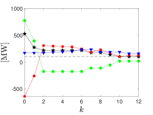
In Figure 3, we report the representative case that $n_{\mu}=3$ and $\Pi(0)$ is the arbitrary one. The power imbalances $P_{1}(k)$, $P_{2}(k)$, $P_{3}(k)$ are depicted in Figure 3(a), while the final partition $\Pi(K)$ is portrayed in Figure 3(b). Interestingly, across all our numerical experiments, not only does our algorithm ensure fulfillment of the bound given in Theorem III.1, but it also always ensures $J(K)=J^{*}$, and in all cases it succeeds in reducing the standard deviation among the power imbalances of the islands with respect to that of the initial partition (see Table II).

Finally, we note that, as shown in Table II, for a given test case and a desired number of islands $n_{\mu}$, there are multiple optimal solutions minimizing $J$. This opens the possibility of developing a multi-objective partitioning strategy, which might be the subject of future study.

Case	$n_{\mu}$	$K$	Cut-set at $\Pi(0)$	$\Pi(0)$	Cut-set at $\Pi(K)$	$J(0)$	$J(K)$	$J^{*}$	$P_{l}(0)$	$P_{l}(K)$	Bound (17)
IEEE 300	3	3	$\begin{array}[]{c}\{3\text{-}129,7\text{-}110,\\ 40\text{-}68,54\text{-}123,\\ 57\text{-}66,66\text{-}190,\\ 67\text{-}190,68\text{-}73,\\ 185\text{-}186\}\end{array}$	SSRP+BFS	$\begin{array}[]{c}\{3\text{-}129,40\text{-}68,\\ 54\text{-}123,57\text{-}66,\\ 64\text{-}67,66\text{-}190,\\ 68\text{-}73,109\text{-}110,\\ 184\text{-}185,185\text{-}187\}\end{array}$	$102.92$	$102.92$	$102.92$	$\begin{array}[]{c}\{6.11,\\ 129.98,\\ 172.65\}\end{array}$	$\begin{array}[]{c}\{6.11,\\ 145.98,\\ 156.65\}\end{array}$	1254.95
IEEE 300	3	12	$\begin{array}[]{c}\{40\text{-}68,57\text{-}66,\\ 66\text{-}190,67\text{-}190,\\ 68\text{-}73,106\text{-}113,\\ 112\text{-}116,122\text{-}123,\\ 185\text{-}186\}\end{array}$	Arbitrary	$\begin{array}[]{c}\{36\text{-}40,39\text{-}40,\\ 61\text{-}66,64\text{-}67,\\ 65\text{-}66,68\text{-}73,\\ 105\text{-}106,106\text{-}107,\\ 106\text{-}147,112\text{-}116,\\ 119\text{-}121,121\text{-}154,\\ 122\text{-}124,122\text{-}128,\\ 127\text{-}157,154\text{-}158,\\ 157\text{-}158,168\text{-}189,\\ 172\text{-}187,177\text{-}188,\\ 184\text{-}185\}\end{array}$	$529.49$	$102.92$	$102.92$	$\begin{array}[]{c}\{-639.87,\\ 775.96,\\ 172.65\}\end{array}$	$\begin{array}[]{c}\{129.21,\\ 18.89,\\ 160.65\}\end{array}$	1254.95
IEEE 300	4	5	$\begin{array}[]{c}\{3\text{-}129,7\text{-}110,\\ 40\text{-}68,54\text{-}123,\\ 61\text{-}66,64\text{-}67\\ 65\text{-}66,68\text{-}73,\\ 68\text{-}173,174\text{-}198,\\ 185\text{-}186\}\end{array}$	SSRP+BFS	$\begin{array}[]{c}\{3\text{-}129,7\text{-}110,\\ 40\text{-}68,54\text{-}123,\\ 57\text{-}180,57\text{-}190,\\ 66\text{-}190,67\text{-}190,\\ 68\text{-}73,68\text{-}173,\\ 168\text{-}187,172\text{-}187,\\ 174\text{-}198,184\text{-}185\}\end{array}$	$77.187$	$77.187$	$77.187$	$\begin{array}[]{c}\{19.76,\\ 6.11,\\ 205.98,\\ 76.9\}\end{array}$	$\begin{array}[]{c}\{114.76,\\ 6.11,\\ 110.98,\\ 76.9\}\end{array}$	1908.2
IEEE 300	4	3	$\begin{array}[]{c}\{57\text{-}66,64\text{-}67,\\ 66\text{-}190,68\text{-}173,\\ 109\text{-}110,109\text{-}129,\\ 122\text{-}123,174\text{-}191,\\ 174\text{-}198,184\text{-}185,\\ 185\text{-}187\}\end{array}$	[26]	$\begin{array}[]{c}\{7\text{-}110,57\text{-}66,\\ 66\text{-}190,67\text{-}190,\\ 68\text{-}173,109\text{-}129\\ 122\text{-}123,168\text{-}187,\\ 172\text{-}187,174\text{-}191,\\ 174\text{-}198,184\text{-}185\}\end{array}$	$77.187$	$77.187$	$77.187$	$\begin{array}[]{c}\{145.98,\\ 79.76,\\ 6.11\\ 76.9\}\end{array}$	$\begin{array}[]{c}\{110.98,\\ 114.76,\\ 6.11,\\ 76.9\}\end{array}$	1908.2

TABLE II: Results after applying Algorithms 1 and 2 to the IEEE 300 test cases, considering different initial partitions $\Pi(0)$. Power values are reported in MW. Note that bound (17) is computed for $k=K$.

(a)

(b)

Figure 3: Partitioning of the IEEE 300 test system into $n_{\mu}=3$ islands, through Algorithms 1 and 2. (a) $P_{1}(k)$ (red squares), $P_{2}(k)$ (green circles), $P_{3}(k)$ (blue triangles), $J(k)$ (black stars), and $J^{*}$ (dashed line). (b) Final network partition $\Pi(K)$; red squares denote $\mathcal{V}_{1}(K)$, green circles denote $\mathcal{V}_{2}(K)$, and blue triangles denote $\mathcal{V}_{3}(K)$. The nodes’ migration order is $106,122,185,187,168,188,127,66,121,158,67$ and $40$.

V Proof of Convergence

To prove Lemma 1 and Theorem III.1 we first need to define the stack vector $\mathbf{P}(k)\coloneqq[P_{1}(k)\ \cdots\ P_{n_{\mu}}(k)]^{\mathsf{T}}$ and $\mathbf{P}^{*}\coloneqq p^{*}\mathbf{1}$, and then give the following Lemma.

Proof.

From (3), we have that

$$J(k)=\frac{1}{n_{\mu}}\left(\sum_{l:P_{l}(k)>0}P_{l}(k)-\sum_{l:P_{l}(k)\leq 0}P_{l}(k)\right).$$ (20)

Moreover, as

$$\sum_{l:P_{l}(k)>0}P_{l}(k)+\sum_{l:P_{l}(k)\leq 0}P_{l}(k)=P_{\text{tot}}=n_{\mu}p^{*},$$

we can recast (20) as

$$J(k)=\frac{1}{n_{\mu}}\left(2\sum_{l:P_{l}(k)>0}P_{l}(k)-n_{\mu}p^{*}\right).$$

Hence, as $J^{*}=|p^{*}|$ [from (4)], we obtain

$$J(k)-J^{*}=\frac{2}{n_{\mu}}\sum_{l:P_{l}(k)>0}P_{l}(k)-(p^{*}+|p^{*}|).$$ (21)

Without loss of generality, let us relabel the islands so that $P_{1}(k)\leq P_{2}(k)\leq\dots\leq P_{n_{\mu}}(k)$. Then, as the graph $\mathcal{G}$ (defined in § II) and all the islands remain connected for all $k$, at each step also the graph $\mathcal{G}^{\Pi(k)}$ (defined in § II) will be connected and thus (16) implies that

$$P_{l+1}(k)\leq P_{l}(k)+\max_{i\in\mathcal{V}}|p_{i}|,\quad\forall l\in\{1,\dots,n_{\mu}-1\}.$$ (22)

Note that, from (2), $\sum_{l=1}^{n_{\mu}}P_{l}(k)=P_{\text{tot}}=n_{\mu}p^{*}$, and hence from (22) we obtain

$$P_{l}(k)\leq p^{*}+\bar{p}\left(l-\frac{n_{\mu}+1}{2}\right),\quad\forall l\in\{1,\dots,n_{\mu}\},$$ (23)

with $\bar{p}\coloneqq\max_{i\in\mathcal{V}}|p_{i}|$. From (21), $J(k)-J^{*}$ is maximized (worst case) when (23) is an equality. In such a case, to compute $J(k)-J^{*}$ by leveraging (21), we must first find

$$l^{*}:\quad P_{l}(k)\geq 0,\ \forall l\in\{l^{*},\dots,n_{\mu}\}.$$ (24)

Hence, to find $l^{*}$ we must find the smallest integer $l$ such that

$$p^{*}+\bar{p}\left(l-\frac{n_{\mu}+1}{2}\right)\geq 0,$$ (25)

yielding (18). Then, from (24), (23), and (21), we obtain (17) and the Lemma is proved. ∎

Now, let us exploit Lemma 1 to prove Theorem III.1.

Proof of Theorem III.1.

Consider a triplet $(l,m,i)$ fulfilling (19), and

$$|P_{m}(k)-P_{l}(k)|>|p_{i}|;$$ (26)

we start by showing that, when assuming (19), (26) is equivalent to (14a), i.e., a migration of node $i$ from island $\mathcal{M}_{m}$ to $\mathcal{M}_{l}$ will occur.

Firstly, we show that (14a) implies (26). When $P_{m}(k)<P_{l}(k)$, we have $p_{i}<0$ from (19b), and from (14a) we have that

$$P_{m}(k)<P_{l}(k+1).$$ (27)

Differently, when $P_{l}(k)<P_{m}(k)$, we have $p_{i}>0$ from (19b), and from (14a) we have that

$$P_{l}(k)<P_{m}(k+1).$$ (28)

From (27) and (28), recalling (15a) and (15b), we have

$$\begin{dcases}P_{m}(k)-P_{l}(k)<p_{i},&\text{if }p_{i}<0,\\ P_{m}(k)-P_{l}(k)>p_{i},&\text{if }p_{i}>0.\end{dcases}$$ (29)

As (29) implies (26), we have proved that (14a) implies (26).

Now, let us prove that (26) implies (14a). To do so, note that (26) is equivalent to

$$\begin{dcases}P_{l}(k)>P_{m}(k)+|p_{i}|,&\text{if }P_{l}(k)>P_{m}(k),\\ P_{m}(k)>P_{l}(k)+|p_{i}|,&\text{if }P_{l}(k)<P_{m}(k).\end{dcases}$$ (30)

Moreover, exploiting (19b) and recalling (15a) and (15b), (30) can be recast as

$$\begin{dcases}P_{m}(k)<P_{l}(k)+p_{i}=P_{l}(k+1),&\text{if }P_{l}(k)>P_{m}(k),\\ P_{l}(k)>P_{m}(k)-p_{i}=P_{m}(k+1),&\text{if }P_{l}(k)<P_{m}(k).\end{dcases}$$ (31)

It is straightforward to see that (31) immediately leads to (14a). Therefore, we have proved that (when (19) holds) $\eqref{eq:comp_cond}\Leftrightarrow\eqref{eq:migration_rule}$.

As (14a) is equivalent to (26) and (19), then if at some step, say $K$, no triplet $(l,m,i)$ existed fulfilling (26), the migration process would stop and, as the network $\mathcal{G}$ is connected and so is the graph $\mathcal{G}^{\Pi(K)}$ at that step, we would have

$$|P_{l}(K)-P_{m}(K)|\leq\max_{i\in\mathcal{V}}|p_{i}|\quad\forall l,m:\mathcal{V}_{m}(K)\cap\mathcal{N}(\mathcal{V}_{l}(K))\neq\varnothing.$$ (32)

As from Lemma 1, (32) implies that the bound (17) holds, to prove our thesis we are left with showing that a stopping time instant $K$ exists. Firstly, note that such a step $K$ exists if (14a) fulfills

$$\left\lVert\mathbf{P}(k+1)-\mathbf{P}^{*}\right\rVert_{2}\leq\alpha\left\lVert\mathbf{P}(k)-\mathbf{P}^{*}\right\rVert_{2}\ \forall k\in\{0,...,K-1\}$$ (33)

for some positive scalar $\alpha<1$ as if (33) were satisfied, then our migration rule would be a contraction mapping. In such case, from the Banach-Caccioppoli theorem [34], there would be no limit cycles in the sequence $\{\mathbf{P}(k)\}$ and thus also in $\{\Pi(k)\}$. Hence, as the number of possible partitions is finite, so would be the sequence $\{\mathbf{P}(k)\}$ and thus, to complete our proof, we need to show that (14a) implies (33). As we have enforced that only one migration occurs at each step $k$, then $\mathbf{P}(k+1)$ only differs from $\mathbf{P}(k)$ for the $l$-th and $m$-th entries. Hence, proving (33) only requires showing that

$$\begin{split}(P_{l}(k+1)-p^{*})^{2}+&(P_{m}(k+1)-p^{*})^{2}\\ &<(P_{l}(k)-p^{*})^{2}+(P_{m}(k)-p^{*})^{2}\end{split}$$ (34)

for all $k\in\{0,...,K-1\}$. After a few algebraic simplifications, (34) can be rewritten as

$$p_{i}(P_{l}(k)-P_{m}(k)+p_{i})<0\quad k\in\{0,...,K-1\},$$ (35)

which is trivially fulfilled by any triplet $(l,m,i)$ fulfilling (19) and (26), yielding that (19) and (26) imply (33). In turn, as (19) and (26) imply (14a), the existence of $K$ and thus our thesis remains proved. ∎

VI Conclusions

We introduced a power network islanding algorithm that solves the Intentional Controlled Islanding problem in a distributed manner. Our strategy allows the network nodes to self-organise so as to minimize the average absolute power imbalance among islands. To allow the nodes to make informed decisions, we devised a consensus-based estimator which is instrumental to the migration process, as it allows nodes to estimate the power imbalances of neighboring islands in a distributed manner. We demonstrated analytically that our algorithm converges in finite time to a partition whose average absolute power imbalance is in a given neighborhood of the optimal one. We tested the strategy on two benchmark power networks, the IEEE 118 and 300 bus systems, after the disconnection of one of their transmission lines showing the effectiveness of the proposed approach.

References

- [1] F. Dörfler, J. W. Simpson-Porco, and F. Bullo, “Breaking the hierarchy: Distributed control and economic optimality in microgrids,” IEEE Transactions on Control of Network Systems, vol. 3, no. 3, pp. 241–253, 2015.
- [2] A. Bidram and A. Davoudi, “Hierarchical structure of microgrids control system,” IEEE Transactions on Smart Grid, vol. 3, no. 4, pp. 1963–1976, 2012.
- [3] P. Frasca, H. Ishii, C. Ravazzi, and R. Tempo, “Distributed randomized algorithms for opinion formation, centrality computation and power systems estimation: A tutorial overview,” European Journal of Control, vol. 24, pp. 2–13, 2015.
- [4] P. Pourbeik, P. S. Kundur, and C. W. Taylor, “The anatomy of a power grid blackout-root causes and dynamics of recent major blackouts,” IEEE Power and Energy Magazine, vol. 4, no. 5, pp. 22–29, 2006.
- [5] J. Rocabert, A. Luna, F. Blaabjerg, and P. Rodriguez, “Control of power converters in ac microgrids,” IEEE Transactions on Power Electronics, vol. 27, no. 11, pp. 4734–4749, 2012.
- [6] A. Tayyebi, D. Groß, A. Anta, F. Kupzog, and F. Dörfler, “Frequency stability of synchronous machines and grid-forming power converters,” IEEE Journal of Emerging and Selected Topics in Power Electronics, vol. 8, no. 2, pp. 1004–1018, 2020.
- [7] C. Arghir, T. Jouini, and F. Dörfler, “Grid-forming control for power converters based on matching of synchronous machines,” Automatica, vol. 95, pp. 273–282, 2018.
- [8] F. Milano, F. Dörfler, G. Hug, D. J. Hill, and G. Verbič, “Foundations and challenges of low-inertia systems,” in 2018 IEEE Power Systems Computation Conference (PSCC), 2018, pp. 1–25.
- [9] F. Dörfler, S. Bolognani, J. W. Simpson-Porco, and S. Grammatico, “Distributed control and optimization for autonomous power grids,” in IEEE 18th European Control Conference (ECC), 2019, pp. 2436–2453.
- [10] G. Lalor, A. Mullane, and M. O’Malley, “Frequency control and wind turbine technologies,” IEEE Transactions on Power Systems, vol. 20, no. 4, pp. 1905–1913, 2005.
- [11] H. Bevrani, A. Ghosh, and G. Ledwich, “Renewable energy sources and frequency regulation: survey and new perspectives,” IET Renewable Power Generation, vol. 4, no. 5, pp. 438–457, 2010.
- [12] A. Ulbig, T. S. Borsche, and G. Andersson, “Impact of low rotational inertia on power system stability and operation,” Proceedings of the 19th World Congress, IFAC Proceedings Volumes, vol. 47, no. 3, pp. 7290–7297, 2014.
- [13] X. Fan, E. Crisostomi, D. Thomopulos, B. Zhang, and S. Yang, “A controlled islanding algorithm for AC/DC hybrid power systems utilizing dc modulation,” IET Generation, Transmission & Distribution, vol. 14, no. 26, pp. 6440–6449, 2020.
- [14] S. Pahwa, M. Youssef, P. Schumm, C. Scoglio, and N. Schulz, “Optimal intentional islanding to enhance the robustness of power grid networks,” Physica A: Statistical Mechanics and its Applications, vol. 392, no. 17, pp. 3741–3754, 2013.
- [15] K. Sun, D.-Z. Zheng, and Q. Lu, “Splitting strategies for islanding operation of large-scale power systems using obdd-based methods,” IEEE Transactions on Power Systems, vol. 18, no. 2, pp. 912–923, 2003.
- [16] M. Adibi, R. Kafka, S. Maram, and L. M. Mili, “On power system controlled separation,” IEEE Transactions on Power Systems, vol. 21, no. 4, pp. 1894–1902, 2006.
- [17] P. Fernández-Porras, M. Panteli, and J. Quirós-Tortós, “Intentional controlled islanding: when to island for power system blackout prevention,” IET Generation, Transmission & Distribution, vol. 12, no. 14, pp. 3542–3549, 2018.
- [18] A. R. H. Ahangar, G. B. Gharehpetian, and H. R. Baghaee, “A review on intentional controlled islanding in smart power systems and generalized framework for ici in microgrids,” International Journal of Electrical Power & Energy Systems, vol. 118, p. 105709, 2020.
- [19] H. Haddadian and R. Noroozian, “Multi-microgrids approach for design and operation of future distribution networks based on novel technical indices,” Applied Energy, vol. 185, pp. 650–663, 2017.
- [20] Z. Wang, B. Chen, J. Wang, M. M. Begovic, and C. Chen, “Coordinated energy management of networked microgrids in distribution systems,” IEEE Transactions on Smart Grid, vol. 6, no. 1, pp. 45–53, 2014.
- [21] S. A. Arefifar and Y. A.-R. I. Mohamed, “Dg mix, reactive sources and energy storage units for optimizing microgrid reliability and supply security,” IEEE Transactions on Smart Grid, vol. 5, no. 4, pp. 1835–1844, 2014.
- [22] S. A. Arefifar, A.-R. M. Yasser, and T. H. El-Fouly, “Optimum microgrid design for enhancing reliability and supply-security,” IEEE Transactions on Smart Grid, vol. 4, no. 3, pp. 1567–1575, 2013.
- [23] S. Hasanvand, M. Nayeripour, E. Waffenschmidt, and H. Fallahzadeh-Abarghouei, “A new approach to transform an existing distribution network into a set of micro-grids for enhancing reliability and sustainability,” Applied Soft Computing, vol. 52, pp. 120–134, 2017.
- [24] S. Mohammadi, S. Soleymani, and B. Mozafari, “Scenario-based stochastic operation management of microgrid including wind, photovoltaic, micro-turbine, fuel cell and energy storage devices,” International Journal of Electrical Power & Energy Systems, vol. 54, pp. 525–535, 2014.
- [25] Z. Liu, A. Clark, L. Bushnell, D. S. Kirschen, and R. Poovendran, “Controlled islanding via weak submodularity,” IEEE Transactions on Power Systems, vol. 34, no. 3, pp. 1858–1868, 2018.
- [26] A. Kyriacou, P. Demetriou, C. Panayiotou, and E. Kyriakides, “Controlled islanding solution for large-scale power systems,” IEEE Transactions on Power Systems, vol. 33, no. 2, pp. 1591–1602, 2017.
- [27] C. Wang, B. Zhang, Z. Hao, J. Shu, P. Li, and Z. Bo, “A novel real-time searching method for power system splitting boundary,” IEEE Transactions on Power Systems, vol. 25, no. 4, pp. 1902–1909, 2010.
- [28] P. Kundur, J. Paserba, V. Ajjarapu, G. Andersson, A. Bose, C. Canizares, N. Hatziargyriou, D. Hill, A. Stankovic, C. Taylor et al., “Definition and classification of power system stability ieee/cigre joint task force on stability terms and definitions,” IEEE Transactions on Power Systems, vol. 19, no. 3, pp. 1387–1401, 2004.
- [29] S. A. Arefifar, Y. A.-R. I. Mohamed, and T. H. M. El-Fouly, “Supply-adequacy-based optimal construction of microgrids in smart distribution systems,” IEEE Transactions on Smart Grid, vol. 3, no. 3, pp. 1491–1502, 2012.
- [30] U. of Washington College of Engineering, “Power systems test case archive,” http://labs.ece.uw.edu/pstca/, accessed: 2021-01-17.
- [31] R. D. Zimmerman, C. E. Murillo-Sánchez, and R. J. Thomas, “Matpower: Steady-state operations, planning, and analysis tools for power systems research and education,” IEEE Transactions on Power Systems, vol. 26, no. 1, pp. 12–19, 2010.
- [32] J. W. Bialek and V. Vahidinasab, “Tree-partitioning as an emergency measure to contain cascading line failures,” IEEE Transactions on Power Systems, vol. 37, no. 1, pp. 467–475, 2021.
- [33] T. H. Cormen, C. E. Leiserson, R. L. Rivest, and C. Stein, Introduction to algorithms. MIT press, 2009.
- [34] W. A. Kirk and B. Sims, “Handbook of metric fixed point theory,” Australian Mathematical Society Gazette, vol. 29, no. 2, 2002.