The study of Kantowski-Sachs perfect fluid cosmological model in modified gravity
T. Vinutha1, K. Niharika1 and K. Sri Kavya2
1
Dept. of Applied Mathematics, AUCST, Andhra University, Visakhapatnam, India.

2 Dept. of Mathematics, Maharaj Vijayaram Gajapathi Raj College of Engineering, Vizianagaram-535005, India.

⋆vinuthatummala@gmail.com

Abstract

Kantowski-Sachs perfect fluid cosmological model is explored in modified gravity with functional form f​(R,T)𝑓𝑅𝑇f(R,T)=f1​(R)subscript𝑓1𝑅f_{1}(R)+f2​(T)subscript𝑓2𝑇f_{2}(T) where R𝑅R is Ricci scalar and T𝑇T is the trace of energy-momentum tensor. With this functional form, three different cases have been formulated, namely negative and positive powers of curvature, logarithmic curvature and exponential curvature given by f1​(R)=R+γ​R2βˆ’ΞΌ4Rsubscript𝑓1𝑅𝑅𝛾superscript𝑅2superscriptπœ‡4𝑅f_{1}(R)=R+\gamma R^{2}-\frac{\mu^{4}}{R}, f1​(R)=R+ν​l​n​(τ​R)subscript𝑓1π‘…π‘…πœˆπ‘™π‘›πœπ‘…f_{1}(R)=R+\nu ln(\tau R) and f1​(R)=R+κ​eβˆ’ΞΉβ€‹Rsubscript𝑓1π‘…π‘…πœ…superscriptπ‘’πœ„π‘…f_{1}(R)=R+\kappa e^{-\iota R} respectively, and for all these three cases, f2​(T)=λ​Tsubscript𝑓2π‘‡πœ†π‘‡f_{2}(T)=\lambda T, here γ𝛾\gamma, Ξ»πœ†\lambda, ΞΌπœ‡\mu, ν𝜈\nu, Ο„πœ\tau, ΞΊπœ…\kappa and ΞΉπœ„\iota are constants. While solving the field equations, two constraints i) Expansion scalar is proportional to shear scalar ii) Hyperbolic scale factor are used. By using these conditions the required optimum solutions are obtained. The physical parameters are calculated and geometrical parameters of three cases are analysed against redshift(z𝑧z) with the help of pictorial representation. In the context of f​(R,T)𝑓𝑅𝑇f(R,T) gravity energy conditions are discussed with the help of pressure and energy density. If strong energy condition is positive the gravity should be attractive but in our model it shows negative it means that cosmic acceleration is due to antigravity, whereas NEC and DEC are fulfilled. The perturbation technique is used to test the stability of the background solutions of the obtained models. The inferences obtained from this paper are in persistent with the present cosmological observations and the model represents an accelerating universe.

Keywords: Kantowski-Sachs spacetime, f​(R,T)𝑓𝑅𝑇f(R,T) theory, perfect fluid.

1 Introduction

Einstein’s theory of general relativity is the foundation of modern physics and it describes black holes and gravitational phenomena but it break down to give an explanation of cosmic acceleration. In recent scenario it is well known that our universe is accelerating[1, 2] and it is one of the trending topics in cosmology. To understand this mysterious concept, we focused on dark energy and modified theories of gravity. The universe is going through an accelerated period of expansion and it is revealed by the experiments such as CMBR and SNI​aπΌπ‘Ž{I}a. Dark energy can be inspected in many ways and reforming the geometric part of the Einstein-Hilbert action is regarded as the most efficient possible way and these changes lead to so many alternative theories of gravity. There are different classes of modified gravity such as f​(R)𝑓𝑅f(R) gravity, f​(T)𝑓𝑇f(T) gravity, f​(G)𝑓𝐺f(G) gravity, f​(R,G)𝑓𝑅𝐺f(R,G) gravity. Among them f​(R)𝑓𝑅f(R) gravity has attracted many researchers because it provides a natural gravitation alternative to dark energy. During the universe expansion f​(R)𝑓𝑅f(R) theory elucidate the change from deceleration phase to acceleration phase. f​(R)𝑓𝑅f(R) theory is presumed to be beneficial for resolution of the hierarchy problem or unification of grand unified theories with gravity in high energy physics. Nojiri and odintsov[3], Nojiri et al.[4], Chatterjee and Jaryal[5], Sotiriou and Faraoni[6] and De Felice and Tsujikawa[7] are some of the authors who worked on various cosmological models in f​(R)𝑓𝑅f(R) theories of gravity. A new class of f​(R,T)𝑓𝑅𝑇f(R,T) gravity presented by Harko et al.[8], by including trace T𝑇T in f​(R)𝑓𝑅f(R) theory. The T𝑇T-dependence in f​(R,T)𝑓𝑅𝑇f(R,T) gravity may appear from the presence of imperfect fluids or quantum effects. Among all the modified theories of gravitation, the f​(R,T)𝑓𝑅𝑇f(R,T) theory is a generalized theory because there is an energy transfer relation between matter and geometry. The existence of this relationship is the cause of the rapid expansion of the universe. The authors who worked on f​(R,T)𝑓𝑅𝑇f(R,T) gravity are included in references [9, 10, 11, 12, 13, 14, 15, 16].
In this paper, we examine three specific cases one of them is combination of 1Rx1superscript𝑅π‘₯\frac{1}{R^{x}} and Rysuperscript𝑅𝑦R^{y} i.e. f​(R)=R+γ​Ryβˆ’ΞΌ4Rx𝑓𝑅𝑅𝛾superscript𝑅𝑦superscriptπœ‡4superscript𝑅π‘₯f(R)=R+\gamma R^{y}-\frac{\mu^{4}}{R^{x}} where γ𝛾\gamma and ΞΌπœ‡\mu are constants. In this functional form, it has both positive and negative curvature powers. At low curvature it leads to gravitational alternative for dark energy which helps in speed up of cosmic expansion where as high curvature describes the inflationary stage of early universe[17]. By considering Rysuperscript𝑅𝑦R^{y} term for 1<y<21𝑦21<y<2 power law inflation happen at early stage. If y=2𝑦2y=2, Starobinsky inflation takes place[18], the term R2superscript𝑅2R^{2} indicates natural correction to general relativity. According to Nojiri and Odinstov[19] R2superscript𝑅2R^{2} term is necessary to get rid of instabilities, linear growth of the gravitational force, produce early time inflation and appear to pass the solar system tests. The state of no linear growth for gravitational force makes it very much fascinating. Higher derivative terms like R2superscript𝑅2R^{2}, R3superscript𝑅3R^{3} can be used to put down the instabilities significantly. For equivalent scalar tensor theory the solar system test may be passed as scalar has large mass originated again by higher derivative terms. The standard Einstein’s gravity may be modified by considering a 1R1𝑅\frac{1}{R} term in the Einstein Hilbert action[20] which represents the present acceleration of the universe. But the insertion of 1R1𝑅\frac{1}{R} term generates instabilities which can be overcome by addition of R2superscript𝑅2R^{2} term to the Einstein’s gravitational action. Besides the advantages of this functional form, have well acceptable Newtonian limit, no instabilities and no Brans Dicke problem in scalar tensor version. When we put y=2𝑦2y=2 and x=1π‘₯1x=1 in the above functional form f​(R)=R+γ​Ryβˆ’ΞΌ4Rx𝑓𝑅𝑅𝛾superscript𝑅𝑦superscriptπœ‡4superscript𝑅π‘₯f(R)=R+\gamma R^{y}-\frac{\mu^{4}}{R^{x}} it reduces to f​(R)=R+γ​R2βˆ’ΞΌ4R𝑓𝑅𝑅𝛾superscript𝑅2superscriptπœ‡4𝑅f(R)=R+\gamma R^{2}-\frac{\mu^{4}}{R} and the obtained results are very efficient. In addition to this functional form by using the linear function of f​(T)=λ​Tπ‘“π‘‡πœ†π‘‡f(T)=\lambda T, we get the final form of f​(R,T)=R+γ​R2βˆ’ΞΌ4R+λ​T𝑓𝑅𝑇𝑅𝛾superscript𝑅2superscriptπœ‡4π‘…πœ†π‘‡f(R,T)=R+\gamma R^{2}-\frac{\mu^{4}}{R}+\lambda T where γ𝛾\gamma, ΞΌπœ‡\mu and Ξ»πœ†\lambda are constants. Vinutha et al. [21] have worked on Kantowski–Sachs perfect fluid cosmological model in R2superscript𝑅2R^{2}- Gravity. Vinutha and Sri Kavya[22] have studied Bianchi type cosmological models in f​(R,T)𝑓𝑅𝑇f(R,T) theory with quadratic functional form. Brookfield[23] have worked on viability of f​(R)𝑓𝑅f(R) theories with additional powers of curvature. Godani and Samanta[24] have studied traversable warmholes on f​(R)𝑓𝑅f(R) gravity where f​(R)=R+α​Rn𝑓𝑅𝑅𝛼superscript𝑅𝑛f(R)=R+\alpha R^{n}. Banik et al.[25] have discussed Bianchi-I cosmological model in f​(R)=Rβˆ’Ξ²Rn𝑓𝑅𝑅𝛽superscript𝑅𝑛f(R)=R-\frac{\beta}{R^{n}} gravity.
Next, we consider logarithmic curvature i.e. f​(R,T)=R+ν​l​n​(τ​R)+λ​Tπ‘“π‘…π‘‡π‘…πœˆπ‘™π‘›πœπ‘…πœ†π‘‡f(R,T)=R+\nu ln(\tau R)+\lambda T where Ο„πœ\tau, ν𝜈\nu and Ξ»πœ†\lambda are constants. As this modified gravity has put forward a gravitational alternative for dark energy, it is quite interesting to work on this particular functional form. In this model logarithmic terms are produced by quantam effects in curved space time. The need for dark energy may be eradicated by this modified gravity and may aid for the fusion of the early time inflation and cosmic acceleration. Nojiri and Odinstov have studied about modified gravity and proposed some functional forms such as l​n​(R)𝑙𝑛𝑅ln(R) or Rβˆ’n​(l​n​R)msuperscript𝑅𝑛superscriptπ‘™π‘›π‘…π‘šR^{-n}(lnR)^{m} and R+γ​Rβˆ’n​(l​n​RΞΌ2)m𝑅𝛾superscript𝑅𝑛superscript𝑙𝑛𝑅superscriptπœ‡2π‘šR+\gamma R^{-n}(ln\frac{R}{\mu^{2}})^{m}[27, 26]. Fayyaz and Shamir[28] have analysed wormhole structures in logarithmic-corrected R2superscript𝑅2R^{2} gravity. Kourosh and Tahereh [29] have discussed phantom-like behavior in f​(R)=R+β​l​o​g​(RΞΌ2)+γ​Rmπ‘“π‘…π‘…π›½π‘™π‘œπ‘”π‘…superscriptπœ‡2𝛾superscriptπ‘…π‘šf(R)=R+\beta log(\frac{R}{\mu^{2}})+\gamma R^{m} gravity.
By appending the torsion scalar component to the exponential f​(R)𝑓𝑅f(R) theory[30, 31, 32, 33, 34], the functional form is f​(R,T)=R+κ​eβˆ’ΞΉβ€‹R+λ​Tπ‘“π‘…π‘‡π‘…πœ…superscriptπ‘’πœ„π‘…πœ†π‘‡f(R,T)=R+\kappa e^{-\iota R}+\lambda T where ΞΊπœ…\kappa, ΞΉπœ„\iota and Ξ»πœ†\lambda are constants. The reason behind choosing this functional form it comes up with the best way of exploring cosmic acceleration. In contrast to the Λ​C​D​MΛ𝐢𝐷𝑀\Lambda CDM model the exponential gravity model has one more parameter included in it and it also permits the relaxation of fine tuning. Vinutha et al. [35] have studied on Bianchi type cosmological models in modified theory with exponential functional form. Paul et al.[36] have worked on accelerating universe in modified theories of gravity. Sahoo et al.[37] have studied on f​(R,T)=f​(R)+λ​Tπ‘“π‘…π‘‡π‘“π‘…πœ†π‘‡f(R,T)=f(R)+\lambda T gravity models as alternatives to cosmic acceleration. Moreas and Sahoo[38] have discussed traversable wormholes by using functional form f​(R,T)=R+γ​eχ​T𝑓𝑅𝑇𝑅𝛾superscriptπ‘’πœ’π‘‡f(R,T)=R+\gamma e^{\chi T} and also with this functional form Moreas et al.[39] studied FRW cosmological model.
When compared to other anisotropic metrics, Kantowski-Sachs model is very simple and easy to analyze. The cosmologies of Kantowski-Sachs metric possess two properties of symmetry such as spherical symmetry and invariance under spatial translation. It describes spatially homogeneous, anisotropic universe and interior of black holes that does not allow a simply transitive group of motions. It is also used to analyze the behavior of the added degrees of freedom in quantum cosmological model. This metric represents three different anisotropic 3+1313+1 dimensional space time and positive curvature models. The study of anisotropic models were nourished by the theoretical studies and observations of CMB which also been extended to modified theories of gravity. Thus this model with an anisotropic nature appeared most appropriate in describing the early stage of the cosmos. some of the authors who worked on Kantowski Sachs model are [40, 41, 42, 43, 44, 45, 46].
This article is organized as follows: In section 2, f​(R,T)𝑓𝑅𝑇f(R,T) gravity field equations are obtained and in section 3 the field equations of power-law, logarithmic and exponential functional forms are solved. Section 4 discusses the physical and geometrical properties of three cases using graphs and section 5 concludes our results.

2 A brief review of f​(R,T)=f1​(R)+f2​(T)𝑓𝑅𝑇subscript𝑓1𝑅subscript𝑓2𝑇f(R,T)=f_{1}(R)+f_{2}(T) model

The final action principle of f​(R,T)𝑓𝑅𝑇f(R,T) gravity which is a function of matter Lagrangian LmsubscriptπΏπ‘šL_{m} is read as

S=∫[116​π​f​(R,T)+Lm]β€‹βˆ’g​d4​x,𝑆delimited-[]116πœ‹π‘“π‘…π‘‡subscriptπΏπ‘šπ‘”superscript𝑑4π‘₯S=\int\left[\frac{1}{16\pi}f(R,T)+L_{m}\right]\sqrt{-g}d^{4}x, (1)

where g𝑔g is the metric determinant of the fundamental tensor gi​jsubscript𝑔𝑖𝑗g_{ij}, f​(R,T)𝑓𝑅𝑇f(R,T) is an arbitrary function of R𝑅R and T𝑇T which is mentioned in the abstract, LmsubscriptπΏπ‘šL_{m} is the usual matter Lagrangian density and we consider G=c=1𝐺𝑐1G=c=1.
By varying the above equation (1) with respect to gi​jsubscript𝑔𝑖𝑗g_{ij},we obtain the field equations of f​(R,T)𝑓𝑅𝑇f(R,T) gravity in covariant tensor form as

fR​(R,T)​Ri​jβˆ’12​f​(R,T)​gi​j+(gi​jβ€‹β–‘βˆ’βˆ‡iβˆ‡j)​fR​(R,T)=8​π​Ti​jβˆ’fT​(R,T)​θi​jβˆ’fT​(R,T)​Ti​j,subscript𝑓𝑅𝑅𝑇subscript𝑅𝑖𝑗12𝑓𝑅𝑇subscript𝑔𝑖𝑗subscript𝑔𝑖𝑗░subscriptβˆ‡π‘–subscriptβˆ‡π‘—subscript𝑓𝑅𝑅𝑇8πœ‹subscript𝑇𝑖𝑗subscript𝑓𝑇𝑅𝑇subscriptπœƒπ‘–π‘—subscript𝑓𝑇𝑅𝑇subscript𝑇𝑖𝑗f_{R}(R,T)R_{ij}-\frac{1}{2}f(R,T)g_{ij}+(g_{ij}\Box-\nabla_{i}\nabla_{j})f_{R}(R,T)=8\pi T_{ij}-f_{T}(R,T)\theta_{ij}-f_{T}(R,T)T_{ij}, (2)

here, βˆ‡isubscriptβˆ‡π‘–\nabla_{i} is the covariant derivative and β–‘=βˆ‡iβˆ‡jβ–‘subscriptβˆ‡π‘–subscriptβˆ‡π‘—\Box=\nabla_{i}\nabla_{j} is the D’Alemberts operator. fR=βˆ‚f​(R,T)βˆ‚Rsubscript𝑓𝑅𝑓𝑅𝑇𝑅f_{R}=\frac{\partial f(R,T)}{\partial R}, fT=βˆ‚f​(R,T)βˆ‚Tsubscript𝑓𝑇𝑓𝑅𝑇𝑇f_{T}=\frac{\partial f(R,T)}{\partial T} and Ri​jsubscript𝑅𝑖𝑗R_{ij} is the Ricci tensor, where

ΞΈi​j=βˆ’2​Ti​j+gi​j​Lmβˆ’2​gl​kβ€‹βˆ‚2Lmβˆ‚gi​j​gl​k.subscriptπœƒπ‘–π‘—2subscript𝑇𝑖𝑗subscript𝑔𝑖𝑗subscriptπΏπ‘š2superscriptπ‘”π‘™π‘˜superscript2subscriptπΏπ‘šsuperscript𝑔𝑖𝑗superscriptπ‘”π‘™π‘˜\theta_{ij}=-2T_{ij}+g_{ij}L_{m}-2g^{lk}\frac{\partial^{2}L_{m}}{\partial{g^{ij}g^{lk}}}. (3)

Here the energy-momentum tensor is considered to be a perfect fluid which is defined as

Ti​j=(p+ρ)​ui​ujβˆ’p​gi​j,subscriptπ‘‡π‘–π‘—π‘πœŒsubscript𝑒𝑖subscript𝑒𝑗𝑝subscript𝑔𝑖𝑗T_{ij}=(p+\rho)u_{i}u_{j}-pg_{ij}, (4)

where uisubscript𝑒𝑖u_{i} denotes four velocity vector in co-moving coordinates i.e. ui=(1,0,0,0)subscript𝑒𝑖1000u_{i}=(1,0,0,0) and ui​uj=1subscript𝑒𝑖superscript𝑒𝑗1u_{i}u^{j}=1. Hence, the components of energy-momentum tensor become Ti​jsubscript𝑇𝑖𝑗T_{ij}=diag(ρ,βˆ’p,βˆ’p,βˆ’p)πœŒπ‘π‘π‘(\rho,-p,-p,-p), where p𝑝p is the pressure and ρ𝜌\rho is the energy density of perfect fluid. Several authors have studied by choosing energy-momentum tensor as perfect fluid which are included in the references[47, 48, 49, 50, 51, 52, 53, 54]. It takes the form by replacing matter Lagrangian as Lm=βˆ’psubscriptπΏπ‘šπ‘L_{m}=-p[55, 56, 57] in equation (3).

ΞΈi​j=βˆ’2​Ti​jβˆ’p​gi​jsubscriptπœƒπ‘–π‘—2subscript𝑇𝑖𝑗𝑝subscript𝑔𝑖𝑗\theta_{ij}=-2T_{ij}-pg_{ij} (5)

Consequently the field equations for f​(R,T)𝑓𝑅𝑇f(R,T) gravity are procured with the aid of T=Οβˆ’3​pπ‘‡πœŒ3𝑝T=\rho-3p in equation (2) as

Gi​j=subscript𝐺𝑖𝑗absent\displaystyle G_{ij}= 1fR​(R,T)[[8Ο€+fT(R,T)]Ti​j+pfT(R,T)gi​j+12[f(R,T)βˆ’RfR(R,T)]gi​j\displaystyle\frac{1}{f_{R}(R,T)}\Big{[}[8\pi+f_{T}(R,T)]T_{ij}+pf_{T}(R,T)g_{ij}+\frac{1}{2}[f(R,T)-Rf_{R}(R,T)]g_{ij} (6)
βˆ’(gi​jβ–‘βˆ’βˆ‡iβˆ‡j)fR(R,T)],\displaystyle-(g_{ij}\Box-\nabla_{i}\nabla_{j})f_{R}(R,T)\Big{]},

where Gi​jsubscript𝐺𝑖𝑗G_{ij} is the Einstein tensor which is expressed as Ri​jβˆ’12​R​gi​jsubscript𝑅𝑖𝑗12𝑅subscript𝑔𝑖𝑗R_{ij}-\frac{1}{2}Rg_{ij}.
Here, we consider the functional form f​(R,T)=f1​(R)+f2​(T)𝑓𝑅𝑇subscript𝑓1𝑅subscript𝑓2𝑇f(R,T)=f_{1}(R)+f_{2}(T) i.e.

f​(R,T)=R+γ​R2βˆ’ΞΌ4R+λ​T𝑓𝑅𝑇𝑅𝛾superscript𝑅2superscriptπœ‡4π‘…πœ†π‘‡f(R,T)=R+\gamma R^{2}-\frac{\mu^{4}}{R}+\lambda T (7)
f​(R,T)=R+ν​l​n​(τ​R)+λ​Tπ‘“π‘…π‘‡π‘…πœˆπ‘™π‘›πœπ‘…πœ†π‘‡f(R,T)=R+\nu ln(\tau R)+\lambda T (8)
f​(R,T)=R+κ​eβˆ’ΞΉβ€‹R+λ​Tπ‘“π‘…π‘‡π‘…πœ…superscriptπ‘’πœ„π‘…πœ†π‘‡f(R,T)=R+\kappa e^{-\iota R}+\lambda T (9)

as case I, II and III respectively.

3 Metric and solutions of the field equations

Now the metric takes the form,

ds2=dt2βˆ’M2(t)dr2βˆ’N2(t)(dΞΈ2+sin2ΞΈdψ2,)ds^{2}=dt^{2}-M^{2}(t)dr^{2}-N^{2}(t)(d\theta^{2}+\sin^{2}\theta d\psi^{2},) (10)

where M𝑀M and N𝑁N are metric potentials and functions of cosmic time t𝑑t only and co-moving coordinates are (r,ΞΈ,ψ)π‘Ÿπœƒπœ“(r,\theta,\psi).

3.1 Case I - (negative and positive powers of curvature)

The functional form f​(R,T)=R+γ​R2βˆ’ΞΌ4R+λ​T𝑓𝑅𝑇𝑅𝛾superscript𝑅2superscriptπœ‡4π‘…πœ†π‘‡f(R,T)=R+\gamma R^{2}-\frac{\mu^{4}}{R}+\lambda T field equations are as follows

1N2+2​NΒ¨N+N2Λ™N2=βˆ’(8​π+3​λ2)​p1+2​R​γ+ΞΌ4R2+λ​ρ2​(1+2​R​γ+ΞΌ4R2)βˆ’(γ​R22+ΞΌ4R)1+2​R​γ+ΞΌ4R2βˆ’(2β€‹Ξ³βˆ’2​μ4R3)1+2​R​γ+ΞΌ4R2​[2​NΛ™N​RΛ™+RΒ¨]βˆ’6​μ4​RΛ™2R41+2​R​γ+ΞΌ4R2.}\hskip-56.9055pt\left.\begin{aligned} \frac{1}{N^{2}}+\frac{2\ddot{N}}{N}+\frac{\dot{N^{2}}}{N^{2}}&=-\frac{(8\pi+\frac{3\lambda}{2})p}{1+2R\gamma+\frac{\mu^{4}}{R^{2}}}+\frac{\lambda\rho}{2(1+2R\gamma+\frac{\mu^{4}}{R^{2}})}-\frac{(\frac{\gamma R^{2}}{2}+\frac{\mu^{4}}{R})}{1+2R\gamma+\frac{\mu^{4}}{R^{2}}}\\ &\hskip 73.97733pt-\frac{(2\gamma-\frac{2\mu^{4}}{R^{3}})}{1+2R\gamma+\frac{\mu^{4}}{R^{2}}}\Big{[}\frac{2\dot{N}}{N}\dot{R}+\ddot{R}\Big{]}-\frac{\frac{6\mu^{4}\dot{R}^{2}}{R^{4}}}{1+2R\gamma+\frac{\mu^{4}}{R^{2}}}.\end{aligned}\right\} (11)
MΒ¨M+NΒ¨N+M˙​NΛ™M​N=βˆ’(8​π+3​λ2)​p1+2​R​γ+ΞΌ4R2+λ​ρ2​(1+2​R​γ+ΞΌ4R2)βˆ’(γ​R22+ΞΌ4R)1+2​R​γ+ΞΌ4R2βˆ’(2β€‹Ξ³βˆ’2​μ4R3)1+2​R​γ+ΞΌ4R2​[(MΛ™M+NΛ™N)​RΛ™+RΒ¨]βˆ’6​μ4​RΛ™2R41+2​R​γ+ΞΌ4R2.}\hskip-56.9055pt\left.\begin{aligned} \frac{\ddot{M}}{M}+\frac{\ddot{N}}{N}+\frac{\dot{M}\dot{N}}{{M}{N}}&=-\frac{(8\pi+\frac{3\lambda}{2})p}{1+2R\gamma+\frac{\mu^{4}}{R^{2}}}+\frac{\lambda\rho}{2(1+2R\gamma+\frac{\mu^{4}}{R^{2}})}-\frac{(\frac{\gamma R^{2}}{2}+\frac{\mu^{4}}{R})}{1+2R\gamma+\frac{\mu^{4}}{R^{2}}}\\ &\hskip 34.14322pt-\frac{(2\gamma-2\frac{\mu^{4}}{R^{3}})}{1+2R\gamma+\frac{\mu^{4}}{R^{2}}}\Big{[}(\frac{\dot{M}}{M}+\frac{\dot{N}}{N})\dot{R}+\ddot{R}\Big{]}-\frac{6\frac{\mu^{4}\dot{R}^{2}}{R^{4}}}{1+2R\gamma+\frac{\mu^{4}}{R^{2}}}.\end{aligned}\right\} (12)
2​M˙​NΛ™M​N+NΛ™2N2+1N2=(8​π+3​λ2)​ρ1+2​R​γ+ΞΌ4R2βˆ’Ξ»β€‹p2​(1+2​R​γ+ΞΌ4R2)βˆ’(γ​R22+ΞΌ4R)1+2​R​γ+ΞΌ4R2βˆ’(2β€‹Ξ³βˆ’2​μ4R3)1+2​R​γ+ΞΌ4R2​[MΛ™M+2​NΛ™N]​RΛ™.}\hskip-56.9055pt\left.\begin{aligned} 2\frac{\dot{M}\dot{N}}{{M}{N}}+\frac{\dot{N}^{2}}{N^{2}}+\frac{1}{N^{2}}&=\frac{(8\pi+\frac{3\lambda}{2})\rho}{1+2R\gamma+\frac{\mu^{4}}{R^{2}}}-\frac{\lambda p}{2(1+2R\gamma+\frac{\mu^{4}}{R^{2}})}-\frac{(\frac{\gamma R^{2}}{2}+\frac{\mu^{4}}{R})}{1+2R\gamma+\frac{\mu^{4}}{R^{2}}}\\ &\hskip 128.0374pt-\frac{(2\gamma-2\frac{\mu^{4}}{R^{3}})}{1+2R\gamma+\frac{\mu^{4}}{R^{2}}}\Big{[}\frac{\dot{M}}{M}+\frac{2\dot{N}}{N}\Big{]}\dot{R}.\end{aligned}\right\} (13)

here dot denotes derivate with respect to t𝑑t.

3.2 Case - II (logarithmic curvature)

Field equations corresponding to the f​(R,T)=R+ν​l​n​(τ​R)+λ​Tπ‘“π‘…π‘‡π‘…πœˆπ‘™π‘›πœπ‘…πœ†π‘‡f(R,T)=R+\nu ln(\tau R)+\lambda T are

1N2+2​NΒ¨N+N2Λ™N2=βˆ’(8​π+3​λ2)​p1+Ξ½R+λ​ρ2​(1+Ξ½R)βˆ’Ξ½β€‹(1βˆ’l​n​(τ​R))2​(1+Ξ½R)+[2​NΛ™N​RΛ™+RΒ¨]​νR21+Ξ½Rβˆ’2​ν​RΛ™2R31+Ξ½R.}\hskip-56.9055pt\left.\begin{aligned} \frac{1}{N^{2}}+\frac{2\ddot{N}}{N}+\frac{\dot{N^{2}}}{N^{2}}&=\frac{-(8\pi+\frac{3\lambda}{2})p}{1+\frac{\nu}{R}}+\frac{\lambda\rho}{2(1+\frac{\nu}{R})}-\frac{\nu(1-ln(\tau R))}{2(1+\frac{\nu}{R})}\\ &\hskip 85.35826pt+\Big{[}\frac{2\dot{N}}{N}\dot{R}+\ddot{R}\Big{]}\frac{\frac{\nu}{R^{2}}}{1+\frac{\nu}{R}}-\frac{\frac{2\nu\dot{R}^{2}}{R^{3}}}{1+\frac{\nu}{R}}.\end{aligned}\right\} (14)
MΒ¨M+NΒ¨N+M˙​NΛ™M​N=βˆ’(8​π+3​λ2)​p1+Ξ½R+λ​ρ2​(1+Ξ½R)βˆ’Ξ½β€‹(1βˆ’l​n​(τ​R))2​(1+Ξ½R)+Ξ½R21+Ξ½R​[(MΛ™M+NΛ™N)​RΛ™+RΒ¨]βˆ’2​ν​RΛ™2R31+Ξ½R.}\hskip-56.9055pt\left.\begin{aligned} \frac{\ddot{M}}{M}+\frac{\ddot{N}}{N}+\frac{\dot{M}\dot{N}}{{M}{N}}&=-\frac{(8\pi+\frac{3\lambda}{2})p}{1+\frac{\nu}{R}}+\frac{\lambda\rho}{2(1+\frac{\nu}{R})}-\frac{\nu(1-ln(\tau R))}{2(1+\frac{\nu}{R})}\\ &\hskip 56.9055pt+\frac{\frac{\nu}{R^{2}}}{1+\frac{\nu}{R}}\Big{[}(\frac{\dot{M}}{M}+\frac{\dot{N}}{N})\dot{R}+\ddot{R}\Big{]}-\frac{\frac{2\nu\dot{R}^{2}}{R^{3}}}{1+\frac{\nu}{R}}.\\ \end{aligned}\right\} (15)
2​M˙​NΛ™M​N+NΛ™2N2+1N2=(8​π+3​λ2)​ρ1+Ξ½Rβˆ’Ξ»β€‹p2​(1+Ξ½R)βˆ’Ξ½β€‹(1βˆ’l​n​(τ​R))2​(1+Ξ½R)+Ξ½R21+Ξ½R​[MΛ™M+2​NΛ™N]​RΛ™.}\hskip-56.9055pt\left.\begin{aligned} 2\frac{\dot{M}\dot{N}}{{M}{N}}+\frac{\dot{N}^{2}}{N^{2}}+\frac{1}{N^{2}}=\frac{(8\pi+\frac{3\lambda}{2})\rho}{1+\frac{\nu}{R}}-\frac{\lambda p}{2(1+\frac{\nu}{R})}-\frac{\nu(1-ln(\tau R))}{2(1+\frac{\nu}{R})}\\ &\hskip-128.0374pt+\frac{\frac{\nu}{R^{2}}}{1+\frac{\nu}{R}}\Big{[}\frac{\dot{M}}{M}+\frac{2\dot{N}}{N}\Big{]}\dot{R}.\end{aligned}\right\} (16)

3.3 Case - III (exponential curvature)

Field equations corresponding to the f​(R,T)=R+κ​eβˆ’ΞΉβ€‹R+λ​Tπ‘“π‘…π‘‡π‘…πœ…superscriptπ‘’πœ„π‘…πœ†π‘‡f(R,T)=R+\kappa e^{-\iota R}+\lambda T are given as follows:

1N2+2​NΒ¨N+N2Λ™N2=βˆ’(8​π+3​λ2)​p1βˆ’ΞΊβ€‹ΞΉβ€‹eβˆ’ΞΉβ€‹R+λ​ρ2​(1βˆ’ΞΊβ€‹ΞΉβ€‹eβˆ’ΞΉβ€‹R)+κ​eβˆ’ΞΉβ€‹R​(1+ι​R)2​(1βˆ’ΞΊβ€‹ΞΉβ€‹eβˆ’ΞΉβ€‹R)βˆ’ΞΊβ€‹ΞΉ2​eβˆ’ΞΉβ€‹R1βˆ’ΞΊβ€‹ΞΉβ€‹eβˆ’ΞΉβ€‹R​[(2​NΛ™N)​RΛ™+RΒ¨]+κ​ι3​eβˆ’ΞΉβ€‹R​RΛ™21βˆ’ΞΊβ€‹ΞΉβ€‹eβˆ’ΞΉβ€‹R.}\left.\begin{aligned} \frac{1}{N^{2}}+\frac{2\ddot{N}}{N}+\frac{\dot{N^{2}}}{N^{2}}&=-\frac{(8\pi+\frac{3\lambda}{2})p}{1-\kappa\iota e^{-\iota R}}+\frac{\lambda\rho}{2(1-\kappa\iota e^{-\iota R})}+\frac{\kappa e^{-\iota R}(1+\iota R)}{2(1-\kappa\iota e^{-\iota R})}\\ &\hskip 28.45274pt-\frac{\kappa\iota^{2}e^{-\iota R}}{1-\kappa\iota e^{-\iota R}}\Big{[}(\frac{2\dot{N}}{N})\dot{R}+\ddot{R}\Big{]}+\frac{\kappa\iota^{3}e^{-\iota R}\dot{R}^{2}}{1-\kappa\iota e^{-\iota R}}.\\ \end{aligned}\right\} (17)
MΒ¨M+NΒ¨N+M˙​NΛ™M​N=βˆ’(8​π+3​λ2)​p1βˆ’ΞΊβ€‹ΞΉβ€‹eβˆ’ΞΉβ€‹R+λ​ρ2​(1βˆ’ΞΊβ€‹ΞΉβ€‹eβˆ’ΞΉβ€‹R)+κ​eβˆ’ΞΉβ€‹R​(1+ι​R)2​(1βˆ’ΞΊβ€‹ΞΉβ€‹eβˆ’ΞΉβ€‹R)βˆ’ΞΊβ€‹ΞΉ2​eβˆ’ΞΉβ€‹R1βˆ’ΞΊβ€‹ΞΉβ€‹eβˆ’ΞΉβ€‹R​[(MΛ™M+NΛ™N)​RΛ™+RΒ¨]+κ​ι3​eβˆ’ΞΉβ€‹R​RΛ™21βˆ’ΞΊβ€‹ΞΉβ€‹eβˆ’ΞΉβ€‹R.}\left.\begin{aligned} \frac{\ddot{M}}{M}+\frac{\ddot{N}}{N}+\frac{\dot{M}\dot{N}}{{M}{N}}&=-\frac{(8\pi+\frac{3\lambda}{2})p}{1-\kappa\iota e^{-\iota R}}+\frac{\lambda\rho}{2(1-\kappa\iota e^{-\iota R})}+\frac{\kappa e^{-\iota R}(1+\iota R)}{2(1-\kappa\iota e^{-\iota R})}\\ &\hskip 5.69046pt-\frac{\kappa\iota^{2}e^{-\iota R}}{1-\kappa\iota e^{-\iota R}}\Big{[}(\frac{\dot{M}}{M}+\frac{\dot{N}}{N})\dot{R}+\ddot{R}\Big{]}+\frac{\kappa\iota^{3}e^{-\iota R}\dot{R}^{2}}{1-\kappa\iota e^{-\iota R}}.\\ \end{aligned}\right\} (18)
2​M˙​NΛ™M​N+NΛ™2N2+1N2=(8​π+3​λ2)​ρ1βˆ’ΞΊβ€‹ΞΉβ€‹eβˆ’ΞΉβ€‹Rβˆ’Ξ»β€‹p2​(1βˆ’ΞΊβ€‹ΞΉβ€‹eβˆ’ΞΉβ€‹R)+κ​eβˆ’ΞΉβ€‹R​(1+ι​R)2​(1βˆ’ΞΊβ€‹ΞΉβ€‹eβˆ’ΞΉβ€‹R)βˆ’ΞΊβ€‹ΞΉ2​eβˆ’ΞΉβ€‹R​RΛ™1βˆ’ΞΊβ€‹ΞΉβ€‹eβˆ’ΞΉβ€‹R​[MΛ™M+2​NΛ™N].}\left.\begin{aligned} 2\frac{\dot{M}\dot{N}}{{M}{N}}+\frac{\dot{N}^{2}}{N^{2}}+\frac{1}{N^{2}}&=\frac{(8\pi+\frac{3\lambda}{2})\rho}{1-\kappa\iota e^{-\iota R}}-\frac{\lambda p}{2(1-\kappa\iota e^{-\iota R})}+\frac{\kappa e^{-\iota R}(1+\iota R)}{2(1-\kappa\iota e^{-\iota R})}\\ &\hskip 56.9055pt-\frac{\kappa\iota^{2}e^{-\iota R}\dot{R}}{1-\kappa\iota e^{-\iota R}}\Big{[}\frac{\dot{M}}{M}+\frac{2\dot{N}}{N}\Big{]}.\end{aligned}\right\} (19)

To obtain solutions for highly non-linear equations is very strenuous and in order to remove such complications we require some constraints.
(i) We consider ΟƒπœŽ\sigma is proportional to ΞΈπœƒ\theta(where ΟƒπœŽ\sigma is the shear scalar and ΞΈπœƒ\theta is the expansion scalar) and it generate linear relationship between two metric potentials in terms of M𝑀M and N𝑁N as

M=Nn,𝑀superscript𝑁𝑛M=N^{n}, (20)

nβ‰ 0,1𝑛01n\not=0,1 is constant. The physical motivation for assuming this condition is that Hubble expansion of the universe may attain isotropy by the observations of the velocity redshift relation for extra galatic sources if the value of ΟƒΞΈπœŽπœƒ\frac{\sigma}{\theta} is constant[58].
(ii) The average scale factor is assumed as a hyperbolic expansion

a(t)=sinh(Ξ±t)1Ξ²,a(t)=\sinh(\alpha t)^{\frac{1}{\beta}}, (21)

where Ξ±>0𝛼0\alpha>0, Ξ²>0𝛽0{\beta}>0 are constants. The consequence of using this scale factor is time dependent deceleration parameter qπ‘žq [59]. This average scale factor tends to zero if tβ†’0→𝑑0t\to 0 and if tβ†’βˆžβ†’π‘‘t\to\infty then a​(t)π‘Žπ‘‘a(t) becomes infinity.
The directional Hubble parameters are

H1=MΛ™MH2=H3=NΛ™N.formulae-sequencesubscript𝐻1˙𝑀𝑀subscript𝐻2subscript𝐻3˙𝑁𝑁H_{1}=\frac{\dot{M}}{M}~{}~{}~{}~{}~{}~{}~{}~{}H_{2}=H_{3}=\frac{\dot{N}}{N}. (22)

The average Hubble parameter is,

H=13​(H1+2​H2).𝐻13subscript𝐻12subscript𝐻2H=\frac{1}{3}(H_{1}+2H_{2}). (23)

By substituting equation (23) in equation (22), we get

H=aΛ™a=13​(MΛ™M+NΛ™N).π»Λ™π‘Žπ‘Ž13˙𝑀𝑀˙𝑁𝑁H=\frac{\dot{a}}{a}=\frac{1}{3}\Big{(}\frac{\dot{M}}{M}+\frac{\dot{N}}{N}\Big{)}. (24)

From equations (20) - (24), we obtain metric potentials of M𝑀M and N𝑁N as

M=(sinh⁑(α​t))3​nβ​(n+2),𝑀superscript𝛼𝑑3𝑛𝛽𝑛2M=(\sinh(\alpha t))^{\frac{3n}{\beta(n+2)}}, (25)
N=(sinh⁑(α​t))3β​(n+2).𝑁superscript𝛼𝑑3𝛽𝑛2N=(\sinh(\alpha t))^{\frac{3}{\beta(n+2)}}.\\ (26)

If tβ†’βˆžβ†’π‘‘t\to\infty then M𝑀M and N𝑁N are nonzero, hence, our model is free from singularity.
Using equations (25) and (26), the Kantowski sachs metric obtained as

d​s2=d​t2βˆ’(sinh⁑(α​t))6​nβ​(n+2)​d​r2βˆ’(sinh⁑(α​t))6β​(n+2)​(d​θ2+sin2⁑θ​dβ€‹Οˆ2).𝑑superscript𝑠2𝑑superscript𝑑2superscript𝛼𝑑6𝑛𝛽𝑛2𝑑superscriptπ‘Ÿ2superscript𝛼𝑑6𝛽𝑛2𝑑superscriptπœƒ2superscript2πœƒπ‘‘superscriptπœ“2ds^{2}=dt^{2}-(\sinh(\alpha t))^{\frac{6n}{\beta(n+2)}}\;dr^{2}-(\sinh(\alpha t))^{\frac{6}{\beta(n+2)}}(d\theta^{2}+\sin^{2}\theta d\psi^{2}). (27)

The above metric represents a perfect fluid Kantowski-Sachs universe in f​(R,T)𝑓𝑅𝑇f(R,T) theory of gravity.

3.4 Pressure and energy density for case I

By solving the equations of (11),(12) and (13) we get the pressure of the model as

p=14​(Ο‡+ΞΎβˆ’2β€‹Ξ·βˆ’Ο•4+2​ϕ5+2​ϕ6βˆ’Ο•7Ο•2βˆ’Ο•1βˆ’Ο‡+ΞΎ+2​η+4​ϕ3+7​ϕ4+2​ϕ5+2​ϕ6+3​ϕ7Ο•1+Ο•2),𝑝14πœ’πœ‰2πœ‚subscriptitalic-Ο•42subscriptitalic-Ο•52subscriptitalic-Ο•6subscriptitalic-Ο•7subscriptitalic-Ο•2subscriptitalic-Ο•1πœ’πœ‰2πœ‚4subscriptitalic-Ο•37subscriptitalic-Ο•42subscriptitalic-Ο•52subscriptitalic-Ο•63subscriptitalic-Ο•7subscriptitalic-Ο•1subscriptitalic-Ο•2\displaystyle p={\frac{1}{4}}\Big{(}{{\frac{\chi+{\xi}-{2}{\eta}-{\phi_{4}}+{2}{\phi_{5}}+{2}{\phi_{6}}-{\phi_{7}}}{\phi_{2}-\phi_{1}}}-{\frac{{\chi}+{\xi}+{2\eta}+{4}{\phi_{3}}+{7}{\phi_{4}}+{2}{\phi_{5}}+{2}{\phi_{6}}+{3}{\phi_{7}}}{\phi_{1}+\phi_{2}}}}\Big{)}, (28)

and the energy density of the model is obtained as

ρ=14​(Ο‡+ΞΎ+2​η+4​ϕ3+7​ϕ4+2​ϕ5+2​ϕ6+3​ϕ7Ο•1+Ο•2+Ο‡+ΞΎβˆ’2β€‹Ξ·βˆ’Ο•4+2​ϕ5+2​ϕ6βˆ’Ο•7Ο•2βˆ’Ο•1),𝜌14πœ’πœ‰2πœ‚4subscriptitalic-Ο•37subscriptitalic-Ο•42subscriptitalic-Ο•52subscriptitalic-Ο•63subscriptitalic-Ο•7subscriptitalic-Ο•1subscriptitalic-Ο•2πœ’πœ‰2πœ‚subscriptitalic-Ο•42subscriptitalic-Ο•52subscriptitalic-Ο•6subscriptitalic-Ο•7subscriptitalic-Ο•2subscriptitalic-Ο•1\displaystyle\rho={\frac{1}{4}}\Big{(}{\frac{{\chi}+{\xi}+{2\eta}+{4}{\phi_{3}}+{7}{\phi_{4}}+{2}{\phi_{5}}+{2}{\phi_{6}}+{3}{\phi_{7}}}{\phi_{1}+\phi_{2}}}+{{\frac{\chi+\xi-{2}{\eta}-{\phi_{4}}+{2}{\phi_{5}}+{2}{\phi_{6}}-{\phi_{7}}}{\phi_{2}-\phi_{1}}}}\Big{)}, (29)

3.5 Pressure and energy density for case II

By solving the equations (14),(15) and (16) we get the expression for pressure is

p=14​(Ο‡+ΞΎβˆ’2​η+Ο•4βˆ’2​ϕ5+4​ϕ6+Ο•7Ο•2βˆ’Ο•1βˆ’Ο‡+ΞΎ+2​η+4​ϕ3βˆ’7​ϕ4βˆ’2​ϕ5+4​ϕ6βˆ’3​ϕ7Ο•1+Ο•2),𝑝14πœ’πœ‰2πœ‚subscriptitalic-Ο•42subscriptitalic-Ο•54subscriptitalic-Ο•6subscriptitalic-Ο•7subscriptitalic-Ο•2subscriptitalic-Ο•1πœ’πœ‰2πœ‚4subscriptitalic-Ο•37subscriptitalic-Ο•42subscriptitalic-Ο•54subscriptitalic-Ο•63subscriptitalic-Ο•7subscriptitalic-Ο•1subscriptitalic-Ο•2\displaystyle p={\frac{1}{4}}\Big{(}{{\frac{\chi+\xi-{2}{\eta}+{\phi_{4}}-{2}{\phi_{5}}+{4}{\phi_{6}}+{\phi_{7}}}{\phi_{2}-\phi_{1}}}-{\frac{{\chi}+{\xi}+{2\eta}+{4}{\phi_{3}}-{7}{\phi_{4}}-{2}{\phi_{5}}+{4}{\phi_{6}}-{3}{\phi_{7}}}{\phi_{1}+\phi_{2}}}}\Big{)}, (30)

and the energy density of the model is obtained as

ρ=14​(Ο‡+ΞΎ+2​η+4​ϕ3βˆ’7​ϕ4βˆ’2​ϕ5+4​ϕ6βˆ’3​ϕ7Ο•1+Ο•2+Ο‡+ΞΎβˆ’2​η+Ο•4βˆ’2​ϕ5+4​ϕ6+Ο•7Ο•2βˆ’Ο•1),𝜌14πœ’πœ‰2πœ‚4subscriptitalic-Ο•37subscriptitalic-Ο•42subscriptitalic-Ο•54subscriptitalic-Ο•63subscriptitalic-Ο•7subscriptitalic-Ο•1subscriptitalic-Ο•2πœ’πœ‰2πœ‚subscriptitalic-Ο•42subscriptitalic-Ο•54subscriptitalic-Ο•6subscriptitalic-Ο•7subscriptitalic-Ο•2subscriptitalic-Ο•1\displaystyle\rho={\frac{1}{4}}\Big{(}{\frac{{\chi}+{\xi}+{2\eta}+{4}{\phi_{3}}-{7}{\phi_{4}}-{2}{\phi_{5}}+{4}{\phi_{6}}-{3}{\phi_{7}}}{\phi_{1}+\phi_{2}}}+{{\frac{\chi+\xi-{2}{\eta}+{\phi_{4}}-{2}{\phi_{5}}+{4}{\phi_{6}}+{\phi_{7}}}{\phi_{2}-\phi_{1}}}}\Big{)}, (31)

3.6 Pressure and energy density for case III

By solving the equations (17), (18) and(19) we get the pressure of the model as

p=14​(Ο‡+ΞΎβˆ’2β€‹Ξ·βˆ’Ο•4+2​ϕ5βˆ’2​ϕ6βˆ’Ο•7Ο•2βˆ’Ο•1βˆ’Ο‡+ΞΎ+2β€‹Ξ·βˆ’4​ϕ3+7​ϕ4+2​ϕ5βˆ’2​ϕ6+3​ϕ7Ο•1+Ο•2),𝑝14πœ’πœ‰2πœ‚subscriptitalic-Ο•42subscriptitalic-Ο•52subscriptitalic-Ο•6subscriptitalic-Ο•7subscriptitalic-Ο•2subscriptitalic-Ο•1πœ’πœ‰2πœ‚4subscriptitalic-Ο•37subscriptitalic-Ο•42subscriptitalic-Ο•52subscriptitalic-Ο•63subscriptitalic-Ο•7subscriptitalic-Ο•1subscriptitalic-Ο•2\displaystyle p={\frac{1}{4}}\Big{(}{{\frac{\chi+\xi-{2}{\eta}-{\phi_{4}}+{2}{\phi_{5}}-{2}{\phi_{6}}-{\phi_{7}}}{\phi_{2}-\phi_{1}}}-{\frac{{\chi}+{\xi}+{2\eta}-{4}{\phi_{3}}+{7}{\phi_{4}}+{2}{\phi_{5}}-{2}{\phi_{6}}+{3}{\phi_{7}}}{\phi_{1}+\phi_{2}}}}\Big{)}, (32)

and the energy density of the model is obtained as

ρ=14​(Ο‡+ΞΎ+2β€‹Ξ·βˆ’4​ϕ3+7​ϕ4+2​ϕ5βˆ’2​ϕ6+3​ϕ7Ο•1+Ο•2+Ο‡+ΞΎβˆ’2β€‹Ξ·βˆ’Ο•4+2​ϕ5βˆ’2​ϕ6βˆ’Ο•7Ο•2βˆ’Ο•1),𝜌14πœ’πœ‰2πœ‚4subscriptitalic-Ο•37subscriptitalic-Ο•42subscriptitalic-Ο•52subscriptitalic-Ο•63subscriptitalic-Ο•7subscriptitalic-Ο•1subscriptitalic-Ο•2πœ’πœ‰2πœ‚subscriptitalic-Ο•42subscriptitalic-Ο•52subscriptitalic-Ο•6subscriptitalic-Ο•7subscriptitalic-Ο•2subscriptitalic-Ο•1\displaystyle\rho={\frac{1}{4}}\Big{(}{\frac{{\chi}+{\xi}+{2\eta}-{4}{\phi_{3}}+{7}{\phi_{4}}+{2}{\phi_{5}}-{2}{\phi_{6}}+{3}{\phi_{7}}}{\phi_{1}+\phi_{2}}}+{{\frac{\chi+\xi-{2}{\eta}-{\phi_{4}}+{2}{\phi_{5}}-{2}{\phi_{6}}-{\phi_{7}}}{\phi_{2}-\phi_{1}}}}\Big{)}, (33)

The values of Ο‡πœ’\chi, ΞΎπœ‰\xi and Ξ·πœ‚\eta are same for all the three cases whereas, the values of Ο•isubscriptitalic-ϕ𝑖\phi_{i}, for i=1 to 7 for the corresponding cases are clearly given in appendix section.

4 Physical and geometrical properties

The average Hubble parameter is

H=αβ​coth⁑(α​t).𝐻𝛼𝛽hyperbolic-cotangent𝛼𝑑H=\frac{\alpha}{\beta}\coth(\alpha t). (34)

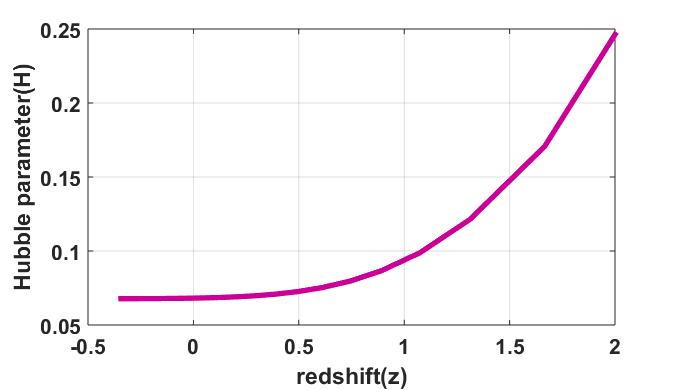
From the figure of Hubble parameter, we trace that it decreases with the decrease of redshift i.e. decreases as time increases. By choosing the values of Ξ±=0.21𝛼0.21\alpha=0.21 and Ξ²=3.10𝛽3.10\beta=3.10 in the scale factor the Hubble parameter is obtained as 0.07G​y​r​sβˆ’1πΊπ‘¦π‘Ÿsuperscript𝑠1Gyr{s^{-1}} which is nearly equal to the present observational data [60]. For this quantity the dimension is 1t​i​m​e1π‘‘π‘–π‘šπ‘’\frac{1}{time}. By using this formula, we can also measure the age of the cosmos.
Refer to caption
Figure 1: Plot of Hubble parameter(H𝐻H) versus redshift(z𝑧z)

(ii) The volume of the model is given by

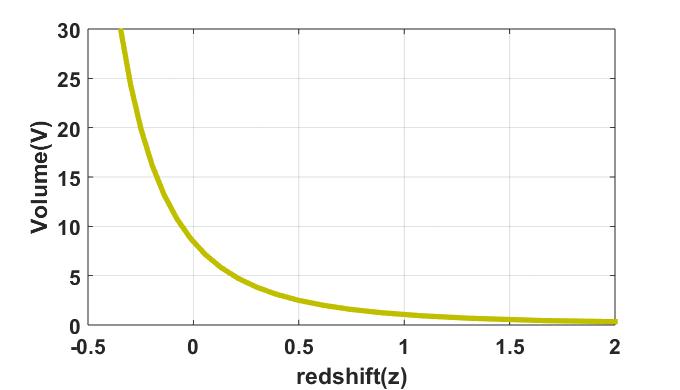
V=a3=(sinh⁑(α​t))3Ξ².𝑉superscriptπ‘Ž3superscript𝛼𝑑3𝛽V=a^{3}=(\sinh(\alpha t))^{\frac{3}{\beta}}. (35)

In figure 2, it is clear that the spatial volume increases with the decrease of redshift i.e. it increases as the time increases and is finite at final epoch.
Refer to caption
Figure 2: Plot of volume(V𝑉V) versus redshift(z𝑧z)

(iii) The expansion scalar ΞΈπœƒ\theta is

ΞΈ=u;ii=3​H=3​α​coth⁑(α​t)Ξ².\theta=u^{i}_{;i}=3H=\frac{3\alpha\coth(\alpha t)}{\beta}. (36)

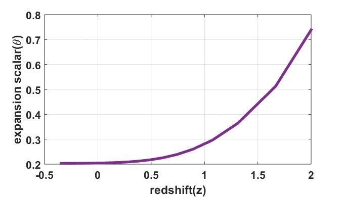
From figure 3, it is observed that expansion scalar decreases with the decrease of redshift i.e. it decreases as time increases. Here we noticed that for t=0𝑑0t=0 the expansion scalar is infinite.

Refer to caption
Figure 3: Plot of expansion scalar(ΞΈπœƒ\theta) versus redshift(z𝑧z)

(iv) We get the shear scalar as

Οƒ2=3​α2​(nβˆ’1)2​coth2⁑(α​t)Ξ²2​(n+2)2,superscript𝜎23superscript𝛼2superscript𝑛12superscripthyperbolic-cotangent2𝛼𝑑superscript𝛽2superscript𝑛22\displaystyle\sigma^{2}=\frac{3\alpha^{2}(n-1)^{2}\coth^{2}(\alpha t)}{\beta^{2}(n+2)^{2}}, (37)

when t=0𝑑0t=0, Οƒ2superscript𝜎2\sigma^{2} (shear scalar) tends to infinity.
(v) The mean anisotropy parameter Ahsubscriptπ΄β„ŽA_{h} is obtained as

Ah=13​[βˆ‘i=13(Hiβˆ’HH)2]subscriptπ΄β„Ž13delimited-[]superscriptsubscript𝑖13superscriptsubscript𝐻𝑖𝐻𝐻2A_{h}=\frac{1}{3}\Big{[}\sum_{i=1}^{3}\Big{(}\frac{H_{i}-H}{H}\Big{)}^{2}\Big{]} (38)

where i=1,2,3𝑖123i=1,2,3 indicate the directional Hubble parameters for the coordinates of r,ΞΈπ‘Ÿπœƒr,\theta and Οˆπœ“\psi. The mean anisotropy parameter is defined on the basis of directional Hubble parameter and mean Hubble parameter.

Ah=2​(nβˆ’1)2(n+2)2;nβ‰ βˆ’2.formulae-sequencesubscriptπ΄β„Ž2superscript𝑛12superscript𝑛22𝑛2A_{h}=\frac{2(n-1)^{2}}{(n+2)^{2}};n\not=-2. (39)

The mean anisotropy parameter Ahsubscriptπ΄β„ŽA_{h} is useful for checking if the model is anisotropic or not. In the present model Ah=0subscriptπ΄β„Ž0A_{h}=0 for n=1𝑛1n=1 and Ahβ‰ 0subscriptπ΄β„Ž0A_{h}\not=0 for nβ‰ 1𝑛1n\not=1 that is the model is anisotropic for nβ‰ 1𝑛1n\not=1 and isotropic for n=1𝑛1n=1.
In all the discussions and graphical representation of physical parameters we constraint the constants for case I as Ξ±=0.21𝛼0.21\alpha=0.21, Ξ²=3.10𝛽3.10\beta=3.10, n=7.38𝑛7.38n=7.38, Ξ»=βˆ’10.02πœ†10.02\lambda=-10.02, ΞΌ=0.2πœ‡0.2\mu=0.2, Ξ³=0.03𝛾0.03\gamma=0.03, case II as Ξ½=0.001𝜈0.001\nu=0.001, Ο„=0.002𝜏0.002\tau=0.002 and case III as ΞΊ=0.2πœ…0.2\kappa=0.2, ΞΉ=0.009πœ„0.009\iota=0.009. The values of parameters α𝛼\alpha, β𝛽\beta, n𝑛n, Ξ»πœ†\lambda in cases II and III are same as that of Case I.
(iv) The deceleration parameter is

q=βˆ’1+dd​t​(1H).π‘ž1𝑑𝑑𝑑1𝐻q=-1+\frac{d}{dt}(\frac{1}{H}). (40)

In this model by using hyperbolic function we obtained deceleration parameter as

q=βˆ’1+β​(1βˆ’tanh2⁑(α​t)).π‘ž1𝛽1superscript2𝛼𝑑\displaystyle q=-1+\beta(1-\tanh^{2}(\alpha t)). (41)

When t<1Ξ±tanhβˆ’1(1βˆ’1Ξ²)12t<\frac{1}{\alpha}\tanh^{-1}(1-\frac{1}{\beta})^{\frac{1}{2}}, qπ‘žq has negative value which represents that the universe is accelerating whereas if t>1Ξ±tanhβˆ’1(1βˆ’1Ξ²)12t>\frac{1}{\alpha}\tanh^{-1}(1-\frac{1}{\beta})^{\frac{1}{2}}, qπ‘žq has positive value which represents that the universe is decelerating. The quantities such as qπ‘žq and H𝐻H specifies the geometric properties of the cosmos.
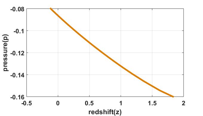
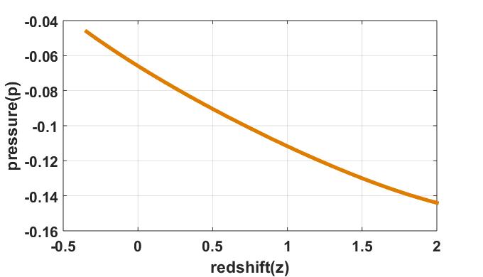
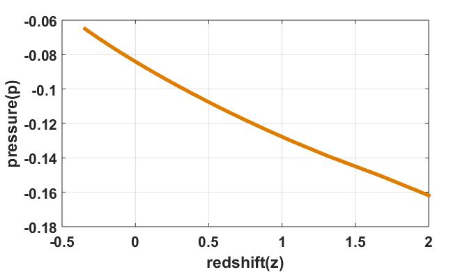
v)Throughout the plots uniform colouring is followed by giving the colours brown for pressure, navy blue for energy density, sky blue for EoS parameter, blue for SEC, green for NEC and red for DEC. Figures 4,5 and 6 illustrate the variation of pressure against redshift in cases I, II and III respectively. The figures shows that in three cases pressure is negative and it is known that a negative pressure fluid is the correct mechanism which is capable of explaining cosmic acceleration within the standard cosmologies, despite the fact that in the latter it is necessary to bring the cosmological constant to get this exotic characteristic. In pressure graphs increase with the decrease of redshift that it is increases as the time increases is perceived which represents cosmic acceleration.
Refer to caption
Figure 4: Pressure(p𝑝p)
in case I
Refer to caption
Figure 5: Pressure(p𝑝p)
in case II
Refer to caption
Figure 6: Pressure(p𝑝p)
in case III

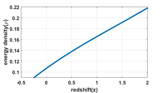
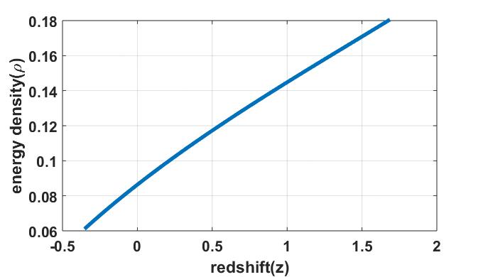
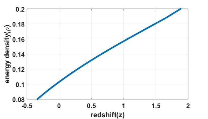
vi) Figures 7,8 and 9 shows the evolution of energy density for cases I, II and III respectively. In all the cases the density decreases with the decrease of redshift i.e. decreases as time increases.
Refer to caption
Figure 7: Energy density(ρ𝜌\rho)
in case I
Refer to caption
Figure 8: Energy density(ρ𝜌\rho)
in case II
Refer to caption
Figure 9: Energy density(ρ𝜌\rho)
in case III

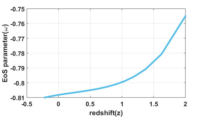
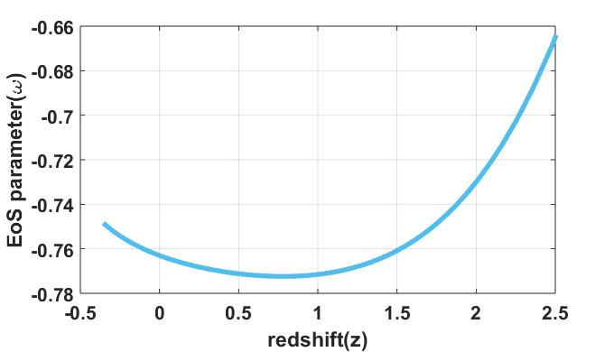
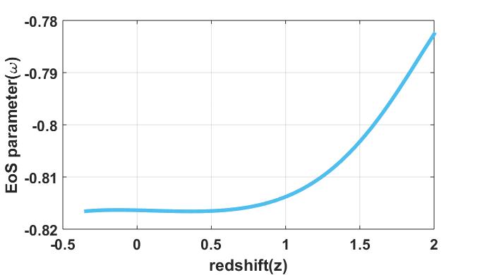
vii) With great efforts the equation of state(EoS) parameter in cosmology of different dark energy models are examined. The parameter relating to the equation of state is a dimensionless term that represents the matter state under some particular physical grounds. In the terminology of p𝑝p and ρ𝜌\rho the EoS can be interpret in the from of Ο‰=pΟπœ”π‘πœŒ\omega=\frac{p}{\rho}. The EoS parameter is distinguished in three regions namely quintessence, phantom, and quintom according to its range. In quintessence region the EoS paramter lies in the range of βˆ’1<Ο‰<βˆ’131πœ”13-1<\omega<-\frac{1}{3}, in phantom phase the EoS parameter is in the range of less than -1 (i.e. Ο‰<βˆ’1πœ”1\omega<-1) and in quintom Ο‰=βˆ’1πœ”1\omega=-1. Figures 10, 11 and 12 of EoS parameter are drawn against redshift and observe that decrease with the decrease of redshift that is decrease as time increases. From the graphs we noticed that our model lies in quintessence region in three cases. According to Planck+nine years WMAP the current value of EoS parameter is approximately as Ο‰=βˆ’1.13βˆ’0.25+0.24πœ”subscriptsuperscript1.130.240.25\omega=-1.13^{+0.24}_{-0.25}[61], and from SNe Ia data with galaxy clustering, CMBR anisotropy statistics the EoS parameter lies in the range βˆ’1.33<Ο‰<βˆ’0.791.33πœ”0.79-1.33<\omega<-0.79, βˆ’1.67<Ο‰<βˆ’0.621.67πœ”0.62-1.67<\omega<-0.62[62] respectively. From the figures of EoS parameters, it is seen that three cases are approximately coincide with observational data which is a good result.
Refer to caption
Figure 10: EoS parameter(Ο‰πœ”\omega)
in case I
Refer to caption
Figure 11: EoS parameter(Ο‰πœ”\omega)
in case II
Refer to caption
Figure 12: EoS parameter(Ο‰πœ”\omega)
in case III

viii)In modified theories of gravity, energy conditions[63, 64, 65] plays a crucial role in studying the behaviour of spacelike and timelike geodesics and these conditions are came from Raychaudhuri equations[66]. Energy conditions can be defined in many ways, such as geometric way and physical way. Moreover energy conditions are significant in the black hole physics, as they lay foundations of the singularity theorems. Another advantage of energy condition is that it allows basic tools to consider certain ideas about black holes and wormholes. There are four most commonly used fundamental energy conditions. The general expressions for energy conditions in regard of pressure and energy density are given below:
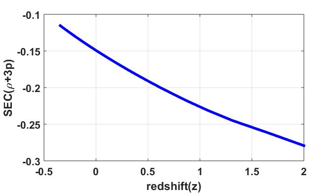
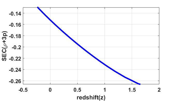
(i)SEC(Strong Energy condition): Gravity always has to be attractive, and in cosmology ρ+3​pβ‰₯0𝜌3𝑝0\rho+3p\geq 0, ρ+pβ‰₯0πœŒπ‘0\rho+p\geq 0 should be observed.
(ii)DEC(Dominant Energy Condition): The energy density should always be positive when measured by any observer that is ρβ‰₯0𝜌0\rho\geq 0, ρ±pβ‰₯0plus-or-minusπœŒπ‘0\rho\pm p\geq 0, must be obeyed.
(iii)WEC(Weak Energy Condition): The energy density must always be positive when measured by any observer that is ρβ‰₯0𝜌0\rho\geq 0, ρ+pβ‰₯0πœŒπ‘0\rho+p\geq 0.
(iv)NEC(Null Energy Condition): NEC is expressed in the form of ρ+pβ‰₯0πœŒπ‘0\rho+p\geq 0 and it ensures the validity of second law of black hole thermodynamics.
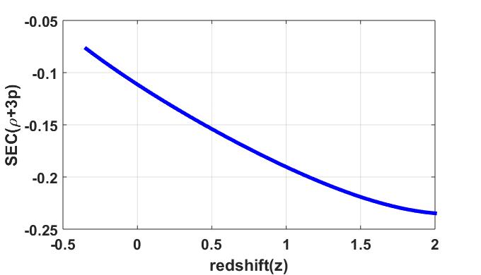
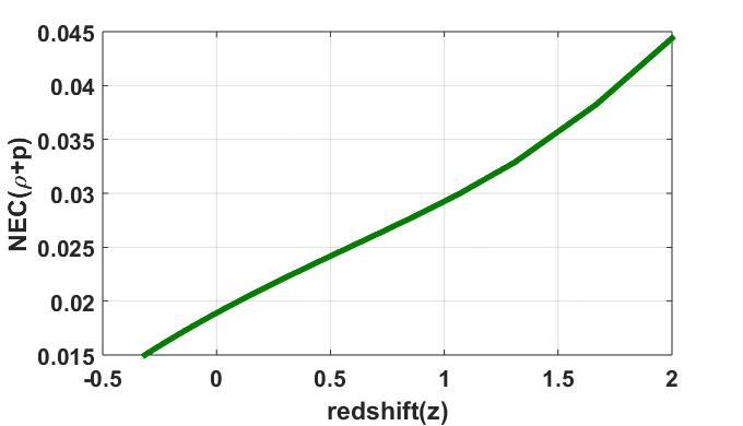
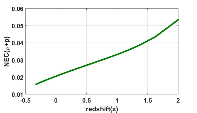
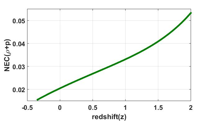
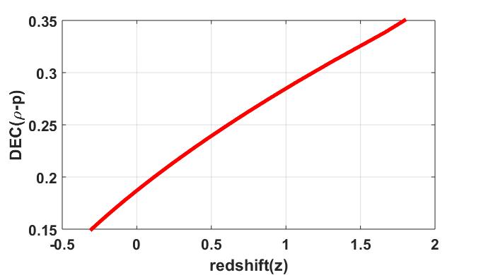
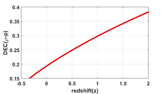
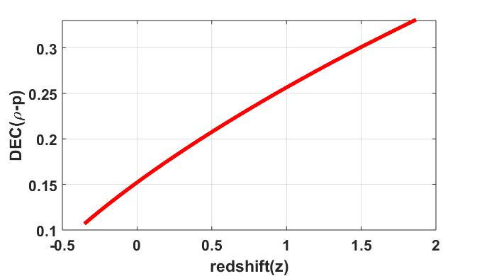
Where NEC, WEC, DEC and SEC represents null, weak, dominant and strong energy conditions. According to present cosmological data to represent the universe with cosmic expansion the SEC of that model should be violated (ρ+3​p≀0𝜌3𝑝0\rho+3p\leq 0). For the obtained models the same scenario can be clearly observed from figures 13 to 15. When compared to strong energy condition null energy condition is more beneficial, as it can be used algebraically due to its weakest pointwise energy condition which results in the strongest theorems and all these energy conditions, are met by electromagnetic field. From figures 16 to 18 it is clear that NEC(ρ+pβ‰₯0πœŒπ‘0\rho+p\geq 0) is satisfied in all the three cases for the obtained model. If NEC satisfies then the parameter EoS occurs in quintessence region. Also from figures 19 to 21 it is clear that DEC (ρ+pβ‰₯0πœŒπ‘0\rho+p\geq 0) is fulfilled in all the three cases for the obtained model.
Refer to caption
Figure 13: SEC in case I
Refer to caption
Figure 14: SEC in case II
Refer to caption
Figure 15: SEC in case III
Refer to caption
Figure 16: NEC in case I
Refer to caption
Figure 17: NEC in case II
Refer to caption
Figure 18: NEC in case III
Refer to caption
Figure 19: DEC in case I
Refer to caption
Figure 20: DEC in case II
Refer to caption
Figure 21: DEC in case III

4.1 Stability analysis

Perturbations are essential for simplify a complex mathematical problems. There are several types of perturbations such as isotropic, anisotropic, homogeneous/inhomogeneous scalar, vector and tensor perturbations. The technique of perturbation is studied as a tool for finding approximate solution and comparing it to the obtained exact solution. Some of the researchers who studied on stability analysis are [67, 68, 69]. Here the stability of solutions in terms of metric perturbation as following

aiβ†’aB​i+δ​ai=aB​i​(1+δ​bi).β†’subscriptπ‘Žπ‘–subscriptπ‘Žπ΅π‘–π›Ώsubscriptπ‘Žπ‘–subscriptπ‘Žπ΅π‘–1𝛿subscript𝑏𝑖a_{i}\to a_{Bi}+\delta a_{i}=a_{Bi}(1+\delta b_{i}). (42)

The perturbation of volume scale factor, directional Hubble factors and mean Hubble factors are

Vβ†’VB+VBβ€‹βˆ‘iδ​bi,ΞΈiβ†’ΞΈB​i+βˆ‘iδ​bi,ΞΈβ†’ΞΈB+13β€‹βˆ‘iδ​bi.formulae-sequence→𝑉subscript𝑉𝐡subscript𝑉𝐡subscript𝑖𝛿subscript𝑏𝑖formulae-sequenceβ†’subscriptπœƒπ‘–subscriptπœƒπ΅π‘–subscript𝑖𝛿subscriptπ‘π‘–β†’πœƒsubscriptπœƒπ΅13subscript𝑖𝛿subscript𝑏𝑖V\to V_{B}+V_{B}\sum_{i}\delta b_{i},\\ \hskip 8.5359pt\theta_{i}\to\theta_{Bi}+\sum_{i}\delta b_{i},\\ \hskip 8.5359pt\theta\to\theta_{B}+\frac{1}{3}\sum_{i}\delta b_{i}. (43)

The following equations are satisfied by the metric perturbation δ​bi𝛿subscript𝑏𝑖\delta b_{i}

βˆ‘iδ​bΒ¨i+2β€‹βˆ‘iΞΈB​i​δ​bΛ™i=0,subscript𝑖𝛿subscript¨𝑏𝑖2subscript𝑖subscriptπœƒπ΅π‘–π›Ώsubscript˙𝑏𝑖0\sum_{i}\delta\ddot{b}_{i}+2\sum_{i}\theta_{Bi}\delta\dot{b}_{i}=0, (44)
δ​bΒ¨i+VΛ™BVB​δ​bΛ™i+βˆ‘jδ​bΛ™j​θB​i=0,𝛿subscript¨𝑏𝑖subscript˙𝑉𝐡subscript𝑉𝐡𝛿subscript˙𝑏𝑖subscript𝑗𝛿subscript˙𝑏𝑗subscriptπœƒπ΅π‘–0\delta\ddot{b}_{i}+\frac{\dot{V}_{B}}{V_{B}}\delta\dot{b}_{i}+\sum_{j}\delta\dot{b}_{j}\theta_{Bi}=0, (45)
βˆ‘iδ​bΛ™i=0.subscript𝑖𝛿subscript˙𝑏𝑖0\sum_{i}\delta\dot{b}_{i}=0. (46)

From equations (44) - (46), we attain

δ​bΒ¨i+VΛ™BVB​δ​bΛ™i=0,𝛿subscript¨𝑏𝑖subscript˙𝑉𝐡subscript𝑉𝐡𝛿subscript˙𝑏𝑖0\delta\ddot{b}_{i}+\frac{\dot{V}_{B}}{V_{B}}\delta\dot{b}_{i}=0, (47)

where VBsubscript𝑉𝐡V_{B} is the background spatial volume and for our case VBsubscript𝑉𝐡V_{B} is

VB=(sinh⁑(α​t))3Ξ².subscript𝑉𝐡superscript𝛼𝑑3𝛽V_{B}=(\sinh(\alpha t))^{\frac{3}{\beta}}. (48)

From above two equations, δ​bi𝛿subscript𝑏𝑖\delta b_{i} is procured as

δ​bi=c1βˆ’c​(β​c​o​s​h2​(α​t)​sech⁑(α​t)​sinhΞ²βˆ’3β⁑(α​t)​F12​(12,Ξ²βˆ’32​β;3​(Ξ²βˆ’1)2​β;βˆ’sinh2⁑(α​t))α​(Ξ²βˆ’3)),𝛿subscript𝑏𝑖subscript𝑐1π‘π›½π‘π‘œπ‘ superscriptβ„Ž2𝛼𝑑sech𝛼𝑑superscript𝛽3𝛽𝛼𝑑subscriptsubscript𝐹1212𝛽32𝛽3𝛽12𝛽superscript2𝛼𝑑𝛼𝛽3\delta b_{i}=c_{1}-c\Big{(}\frac{\beta\sqrt{cosh^{2}(\alpha t)}\operatorname{sech}(\alpha t)\sinh^{\frac{\beta-3}{\beta}}(\alpha t){}_{2}F_{1}{\left(\frac{1}{2},\frac{\beta-3}{2\beta};\frac{3(\beta-1)}{2\beta};-\sinh^{2}(\alpha t)\right)}}{\alpha(\beta-3)}\Big{)}, (49)

where c1subscript𝑐1c_{1} and c𝑐c are integrating constants.
consequently, the actual fluctuations δ​ai=aB​i​δ​bi𝛿subscriptπ‘Žπ‘–subscriptπ‘Žπ΅π‘–π›Ώsubscript𝑏𝑖\delta a_{i}=a_{Bi}\delta b_{i} is

δ​ai=[c1βˆ’c​(β​c​o​s​h2​(α​t)​sech⁑(α​t)​sinhΞ²βˆ’3β⁑(α​t)​F12​(12,Ξ²βˆ’32​β;3​(Ξ²βˆ’1)2​β;βˆ’sinh2⁑(α​t))α​(Ξ²βˆ’3))]​(sinh⁑(α​t))βˆ’3Ξ².𝛿subscriptπ‘Žπ‘–delimited-[]subscript𝑐1π‘π›½π‘π‘œπ‘ superscriptβ„Ž2𝛼𝑑sech𝛼𝑑superscript𝛽3𝛽𝛼𝑑subscriptsubscript𝐹1212𝛽32𝛽3𝛽12𝛽superscript2𝛼𝑑𝛼𝛽3superscript𝛼𝑑3𝛽\delta a_{i}=\Big{[}c_{1}-c\Big{(}\frac{\beta\sqrt{cosh^{2}(\alpha t)}\operatorname{sech}(\alpha t)\sinh^{\frac{\beta-3}{\beta}}(\alpha t){}_{2}F_{1}{\left(\frac{1}{2},\frac{\beta-3}{2\beta};\frac{3(\beta-1)}{2\beta};-\sinh^{2}(\alpha t)\right)}}{\alpha(\beta-3)}\Big{)}\Big{]}(\sinh(\alpha t))^{\frac{-3}{\beta}}. (50)
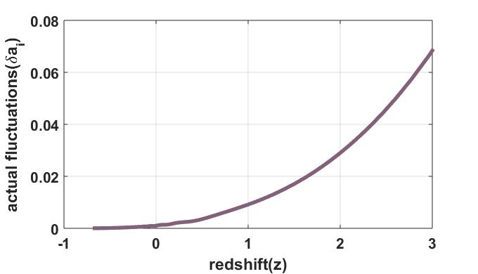
Refer to caption
Figure 22: Plot of actual fluctuations(δ​ai𝛿subscriptπ‘Žπ‘–\delta a_{i}) versus redshift(z𝑧z)

Figure 22 shows the behaviour of actual fluctuations versus redshift and it is noticed that it is a decreasing function with the decrease of redshift that is decreases as time increases. It is clear that δ​aiβ†’0→𝛿subscriptπ‘Žπ‘–0\delta a_{i}\to 0 as zβ†’βˆ’βˆžβ†’π‘§z\to-\infty and hence the background solution is shown to be stable against perturbation of gravitational field.

5 Conclusions

A cosmological model in f​(R,T)𝑓𝑅𝑇f(R,T) theory with three cases namely power law, logarithmic and exponential curvature is obtained. Hyperbolic scale factor is used to solve the field equations to get the solution in each case. The solutions of these field equations represent accelerating model of the universe. The graph of all parameters are drawn against redshift. In graphs the negative region of z𝑧z represents future epoch, positive region of z𝑧z represents past and z=0𝑧0z=0 indicates present. Obtained models are anisotropic and free from singularity all the way through the universe’s evolution. By analyzing all the parameters the conclusions are as follows:

  • β€’

    From figures 1 and 3 and from the equations (34) and (36) it can be seen that Hubble parameter and expansion scalar decreases with the decrease of redshift, and also it is clear that the Hubble parameter and expansion scalar are close to zero when tβ†’βˆžβ†’π‘‘t\to\infty.

  • β€’

    From figure 2 it is clear that volume increases with the decrease of redshift which indicates volume of the expanding universe. From equation (37), it is noticed that the shear scalar is a function of time and tends to zero when tβ†’βˆžβ†’π‘‘t\to\infty.

  • β€’

    From equation (39), the anisotropic parameter is independent of time and Ahβ‰ 0subscriptπ΄β„Ž0A_{h}\not=0 for nβ‰ 1𝑛1n\not=1, Ah=0subscriptπ΄β„Ž0A_{h}=0 for n=1𝑛1n=1. But in this paper due to power law n𝑛n is different from one. Hence the models are anisotropic throughout.

  • β€’

    From the graphs of pressure and energy density of all the three cases, it is clear that the pressure and energy density are negative and positive respectively. Due to the negative pressure and positive energy density the universe is going through accelerating expansion.

  • β€’

    The behavior of EoS parameter against redshift is represented in plots 11 to 13. From these graphs it is obvious that the model is in the quintessence region in three cases that is βˆ’1<Ο‰<βˆ’131πœ”13-1<\omega<-\frac{1}{3} which matches with present observational data.

  • β€’

    In three cases, SEC is violated whereas NEC and DEC are fufilled. The violation of SEC leads to cosmic acceleration which is in good agreement with the expansion of the cosmos.

  • β€’

    As seen in the graph of stability analysis, the actual fluctuations begin with a small positive value and decreases to zero. As a result, the background solution is stable when the gravitational field is perturbed.

A detailed discussion is provided through the obtained models for describing cosmic acceleration. Finally, through the detailed study of the models in three cases namely power law curvature f​(R,T)=R+γ​R2βˆ’ΞΌ4R+λ​T𝑓𝑅𝑇𝑅𝛾superscript𝑅2superscriptπœ‡4π‘…πœ†π‘‡f(R,T)=R+\gamma R^{2}-\frac{\mu^{4}}{R}+\lambda T, logarithmic curvaturef​(R,T)=R+ν​l​n​(τ​R)+λ​Tπ‘“π‘…π‘‡π‘…πœˆπ‘™π‘›πœπ‘…πœ†π‘‡f(R,T)=R+\nu ln(\tau R)+\lambda T and exponential curvature f​(R,T)=R+κ​eβˆ’ΞΉβ€‹R+λ​Tπ‘“π‘…π‘‡π‘…πœ…superscriptπ‘’πœ„π‘…πœ†π‘‡f(R,T)=R+\kappa e^{-\iota R}+\lambda T very good results which represents the universe accelerating expansion are observed. Moreover all the parameters discussed here matches with the recent observational data. At last, without existence of any exotic fluid, the current universe is accelerating is perceived in this paper which is a great outcome. As a future work, this work can be extended to other anisotropic models and can study the similarities and differences between them.

6 Appendix

The values of Ο‡πœ’\chi, ΞΎπœ‰\xi, Ξ·πœ‚\eta are same for all the three cases and are given below

Ο‡=Ο±1Ο±2πœ’subscriptitalic-Ο±1subscriptitalic-Ο±2\displaystyle\hskip-227.62204pt\chi=\frac{\varrho_{1}}{\varrho_{2}}

where

Ο±1=Ξ²2sinh(Ξ±t)2(cosh(Ξ±t)βˆ’1)(cosh(Ξ±t)+1)(n+2)2sinh(Ξ±t)βˆ’6+(βˆ’2​nβˆ’4)​ββ​(n+2)\displaystyle\hskip-85.35826pt\varrho_{1}=\beta^{2}\sinh(\alpha t)^{2}(\cosh(\alpha t)-1)(\cosh(\alpha t)+1)(n+2)^{2}\sinh(\alpha t)^{\frac{-6+(-2n-4)\beta}{\beta(n+2)}}
βˆ’6​(βˆ’9cosh(Ξ±t)22+β​(n+2))​α2\displaystyle-6(\frac{-9\cosh(\alpha t)^{2}}{2}+\beta(n+2))\alpha^{2}
Ο±2=Ξ²2(n+2)2sinh(Ξ±t)2\displaystyle\hskip-227.62204pt\varrho_{2}=\beta^{2}(n+2)^{2}\sinh(\alpha t)^{2}
ΞΎ=Ο±3Ο±2πœ‰subscriptitalic-Ο±3subscriptitalic-Ο±2\displaystyle\hskip-227.62204pt\xi=\frac{\varrho_{3}}{\varrho_{2}}

where

Ο±3=βˆ’3((βˆ’3n2βˆ’3nβˆ’3)cosh(Ξ±t)2+Ξ²(n+2)(n+1))Ξ±2\displaystyle\hskip-165.02606pt\varrho_{3}=-3\Big{(}(-3n^{2}-3n-3)\cosh(\alpha t)^{2}+\beta(n+2)(n+1)\Big{)}\alpha^{2}
Ξ·=Ο±4Ο±2πœ‚subscriptitalic-Ο±4subscriptitalic-Ο±2\displaystyle\hskip-227.62204pt\eta=\frac{\varrho_{4}}{\varrho_{2}}
Ο±4=Ξ²2sinh(Ξ±t)2(cosh(Ξ±t)βˆ’1)(cosh(Ξ±t)+1)(n+2)2sinh(Ξ±t)βˆ’6+(βˆ’2​nβˆ’4)​ββ​(n+2)\displaystyle\hskip-85.35826pt\varrho_{4}=\beta^{2}\sinh(\alpha t)^{2}(\cosh(\alpha t)-1)(\cosh(\alpha t)+1)(n+2)^{2}\sinh(\alpha t)^{\frac{-6+(-2n-4)\beta}{\beta(n+2)}}
+18Ξ±2(n+12)cosh(Ξ±t)2\displaystyle+18\alpha^{2}(n+\frac{1}{2})\cosh(\alpha t)^{2}

For case(i) The values of Ο•1subscriptitalic-Ο•1\phi_{1}, Ο•2subscriptitalic-Ο•2\phi_{2}, Ο•3subscriptitalic-Ο•3\phi_{3}, Ο•4subscriptitalic-Ο•4\phi_{4}, Ο•5subscriptitalic-Ο•5\phi_{5}, Ο•6subscriptitalic-Ο•6\phi_{6} and Ο•7subscriptitalic-Ο•7\phi_{7} are given below

Ο•1​(t)=Ο±5Ο±6subscriptitalic-Ο•1𝑑subscriptitalic-Ο±5subscriptitalic-Ο±6\displaystyle\hskip-227.62204pt\phi_{1}(t)=\frac{\varrho_{5}}{\varrho_{6}}

where

Ο±5(t)=288(n+2)2sinh(Ξ±t)6+(2​n+4)​ββ​(n+2)Ξ²2(βˆ’((n+2)2Ξ²βˆ’3n2βˆ’6nβˆ’9)Ξ±2cosh(Ξ±t)2sinh(Ξ±t)6β​(n+2)\displaystyle\hskip 17.07182pt\varrho_{5}(t)=288(n+2)^{2}\sinh(\alpha t)^{\frac{6+(2n+4)\beta}{\beta(n+2)}}\beta^{2}\Big{(}-\Big{(}(n+2)^{2}\beta-3n^{2}-6n-9\Big{)}\alpha^{2}\cosh(\alpha t)^{2}\sinh(\alpha t)^{\frac{6}{\beta(n+2)}}
+(Ξ±2sinh(Ξ±t)6+(2​n+4)​ββ​(n+2)+cosh(Ξ±t)2Ξ²3βˆ’Ξ²3)(n+2)2Ξ²)2(Ο€+3​λ16)\displaystyle+\Big{(}\alpha^{2}\sinh(\alpha t)^{\frac{6+(2n+4)\beta}{\beta(n+2)}}+\frac{\cosh(\alpha t)^{2}\beta}{3}-\frac{\beta}{3}\Big{)}(n+2)^{2}\beta\Big{)}^{2}(\pi+\frac{3\lambda}{16})
Ο±6​(t)subscriptitalic-Ο±6𝑑\displaystyle\hskip-136.5733pt\varrho_{6}(t) =Ο±7​(t)+4​(cosh⁑(α​t)βˆ’1)​(n+2)2​β2​(cosh⁑(α​t)+1)​ϱ8​(t)absentsubscriptitalic-Ο±7𝑑4𝛼𝑑1superscript𝑛22superscript𝛽2𝛼𝑑1subscriptitalic-Ο±8𝑑\displaystyle=\varrho_{7}(t)+4(\cosh(\alpha t)-1)(n+2)^{2}\beta^{2}(\cosh(\alpha t)+1)\varrho_{8}(t)
Ο±7(t)=((ΞΌ4(n+2)6Ξ²6+324Ξ±4(n+2)2(n2+2n+3)2Ξ²2βˆ’11664Ξ±6(n2+2n+3)3Ξ³)cosh(Ξ±t)6βˆ’3(n+2)2Ξ²(ΞΌ4(n+2)4Ξ²5+72Ξ±4(n2+2n+3)(n+2)2Ξ²2+108Ξ±4(n2+2n+3)2Ξ²βˆ’3888Ξ±6(n2+2n+3)2Ξ³)cosh(Ξ±t)4+3(n+2)4Ξ²2(ΞΌ4(n+2)2Ξ²4+12Ξ±4(n+2)2Ξ²2+72Ξ±4(n2+2n+3)Ξ²βˆ’1296Ξ±6(n2+2n+3)Ξ³)cosh(Ξ±t)2βˆ’Ξ²3(n+2)6(βˆ’432Ξ±6Ξ³+ΞΌ4Ξ²3+36Ξ±4Ξ²))sinh(Ξ±t)18β​(n+2)}\left.\begin{aligned} \hskip 17.07182pt\varrho_{7}(t)=\Big{(}\Big{(}\mu^{4}(n+2)^{6}\beta^{6}+324\alpha^{4}(n+2)^{2}(n^{2}+2n+3)^{2}\beta^{2}-11664\alpha^{6}(n^{2}+2n+3)^{3}\gamma\Big{)}\\ &\hskip-386.95764pt\cosh(\alpha t)^{6}-3(n+2)^{2}\beta\Big{(}\mu^{4}(n+2)^{4}\beta^{5}+72\alpha^{4}(n^{2}+2n+3)(n+2)^{2}\beta^{2}+108\alpha^{4}\\ &\hskip-386.95764pt(n^{2}+2n+3)^{2}\beta-3888\alpha^{6}(n^{2}+2n+3)^{2}\gamma\Big{)}\cosh(\alpha t)^{4}+3(n+2)^{4}\beta^{2}\Big{(}\mu^{4}(n+2)^{2}\beta^{4}\\ &\hskip-386.95764pt+12\alpha^{4}(n+2)^{2}\beta^{2}+72\alpha^{4}(n^{2}+2n+3)\beta-1296\alpha^{6}(n^{2}+2n+3)\gamma\Big{)}\cosh(\alpha t)^{2}\\ &\hskip-369.88582pt-\beta^{3}(n+2)^{6}(-432\alpha^{6}\gamma+\mu^{4}\beta^{3}+36\alpha^{4}\beta)\Big{)}\sinh(\alpha t)^{\frac{18}{\beta(n+2)}}\end{aligned}\right\}
Ο±8(t)=βˆ’6((βˆ’3n2βˆ’6nβˆ’9)cosh(Ξ±t)2+(n+2)2Ξ²)Ξ±2((βˆ’54Ξ±2(n2+2n+3)Ξ³+Ξ²2(n+2)2)cosh(Ξ±t)2βˆ’Ξ²(n+2)2(βˆ’18Ξ±2Ξ³+Ξ²))sinh(Ξ±t)12β​(n+2)+(n+2)2Ξ²2(cosh(Ξ±t)βˆ’1)(cosh(Ξ±t)+1)(((βˆ’108Ξ±2(n2+2n+3)Ξ³+Ξ²2(n+2)2)cosh(Ξ±t)2βˆ’Ξ²(n+2)2(βˆ’36Ξ±2Ξ³+Ξ²))sinh(Ξ±t)6β​(n+2)βˆ’4Ξ²2Ξ³(cosh(Ξ±t)βˆ’1)(cosh(Ξ±t)+1)(n+2)2))}\left.\begin{aligned} \hskip 17.07182pt\varrho_{8}(t)=-6\Big{(}(-3n^{2}-6n-9)\cosh(\alpha t)^{2}+(n+2)^{2}\beta\Big{)}\alpha^{2}\Big{(}(-54\alpha^{2}(n^{2}+2n+3)\gamma\\ &\hskip-358.50488pt+\beta^{2}(n+2)^{2})\cosh(\alpha t)^{2}-\beta(n+2)^{2}(-18\alpha^{2}\gamma+\beta)\Big{)}\sinh(\alpha t)^{\frac{12}{\beta(n+2)}}+(n+2)^{2}\beta^{2}\\ &\hskip-358.50488pt(\cosh(\alpha t)-1)(\cosh(\alpha t)+1)\Big{(}((-108\alpha^{2}(n^{2}+2n+3)\gamma+\beta^{2}(n+2)^{2})\cosh(\alpha t)^{2}\\ &\hskip-358.50488pt-\beta(n+2)^{2}(-36\alpha^{2}\gamma+\beta))\sinh(\alpha t)^{\frac{6}{\beta(n+2)}}-4\beta^{2}\gamma(\cosh(\alpha t)-1)(\cosh(\alpha t)+1)(n+2)^{2})\Big{)}\end{aligned}\right\}
Ο•2​(t)=Ο±9​(t)Ο±6​(t)subscriptitalic-Ο•2𝑑subscriptitalic-Ο±9𝑑subscriptitalic-Ο±6𝑑\displaystyle\hskip-216.2411pt\phi_{2}(t)=\frac{\varrho_{9}(t)}{\varrho_{6}(t)}

where

Ο±9​(t)subscriptitalic-Ο±9𝑑\displaystyle\varrho_{9}(t) =Ξ»18(n+2)2sinh(Ξ±t)6+(2​n+4)​ββ​(n+2)Ξ²2(βˆ’((n+2)2Ξ²βˆ’3n2βˆ’6nβˆ’9)Ξ±2cosh(Ξ±t)2\displaystyle=\lambda 18(n+2)^{2}\sinh(\alpha t)^{\frac{6+(2n+4)\beta}{\beta(n+2)}}\beta^{2}\Big{(}-\Big{(}(n+2)^{2}\beta-3n^{2}-6n-9\Big{)}\alpha^{2}\cosh(\alpha t)^{2}
sinh(Ξ±t)6β​(n+2)+(n+2)2Ξ²(Ξ±2sinh(Ξ±t)6+(2​n+4)​ββ​(n+2)+Ξ²sinh(Ξ±t)23))2\displaystyle\hskip 17.07182pt\sinh(\alpha t)^{\frac{6}{\beta(n+2)}}+(n+2)^{2}\beta\Big{(}\alpha^{2}\sinh(\alpha t)^{\frac{6+(2n+4)\beta}{\beta(n+2)}}+\frac{\beta\sinh(\alpha t)^{2}}{3}\Big{)}\Big{)}^{2}
Ο•3​(t)=Ο±10Ο±13subscriptitalic-Ο•3𝑑subscriptitalic-Ο±10subscriptitalic-Ο±13\displaystyle\hskip-196.32384pt\phi_{3}(t)=\frac{\varrho_{10}}{\varrho_{13}}

where

Ο±10​(t)subscriptitalic-Ο±10𝑑\displaystyle\hskip-82.51282pt\varrho_{10}(t) =βˆ’2​(Ο±11βˆ’Ο±12+Ξ²2​(cosh⁑(α​t)βˆ’1)​(cosh⁑(α​t)+1)​(n+2)2)absent2subscriptitalic-Ο±11subscriptitalic-Ο±12superscript𝛽2𝛼𝑑1𝛼𝑑1superscript𝑛22\displaystyle=-2\Big{(}\varrho_{11}-\varrho_{12}+\beta^{2}(\cosh(\alpha t)-1)(\cosh(\alpha t)+1)(n+2)^{2}\Big{)}
Ο±11(t)=((ΞΌ4(n+2)6Ξ²6βˆ’2916Ξ±6Ξ³(n2+2n+3)3)cosh(Ξ±t)6)βˆ’3Ξ²(n+2)2(ΞΌ4(n+2)4Ξ²5βˆ’972Ξ±6Ξ³(n2+n+3)2)cosh(Ξ±t)4+3(ΞΌ4(n+2)4Ξ²4βˆ’324Ξ±6Ξ³(n2+2n+3))Ξ²2(n+2)4cosh(Ξ±t)2βˆ’Ξ²3(n+2)6(βˆ’108Ξ±6Ξ³+Ξ²3ΞΌ4))sinh(Ξ±t)18β​(n+2)}\left.\begin{aligned} \hskip 25.6073pt\varrho_{11}(t)=\Big{(}\Big{(}\mu^{4}(n+2)^{6}\beta^{6}-2916\alpha^{6}\gamma(n^{2}+2n+3)^{3}\Big{)}\cosh(\alpha t)^{6})-3\beta(n+2)^{2}\Big{(}\mu^{4}(n+2)^{4}\beta^{5}\\ &\hskip-415.4104pt-972\alpha^{6}\gamma(n^{2}+n+3)^{2}\Big{)}\cosh(\alpha t)^{4}+3\Big{(}\mu^{4}(n+2)^{4}\beta^{4}-324\alpha^{6}\gamma(n^{2}+2n+3)\Big{)}\beta^{2}\\ &\hskip-415.4104pt(n+2)^{4}\cosh(\alpha t)^{2}-\beta^{3}(n+2)^{6}(-108\alpha^{6}\gamma+\beta^{3}\mu^{4})\Big{)}\sinh(\alpha t)^{\frac{18}{\beta(n+2)}}\end{aligned}\right\}
Ο±12(t)=108Ξ²2(n+2)2Ξ³(cosh(Ξ±t)+1)((βˆ’3n2βˆ’6nβˆ’9)cosh(Ξ±t)2+(n+2)2Ξ²)2Ξ±4(cosh(Ξ±t)βˆ’1)sinh(Ξ±t)12β​(n+2)+36Ξ²4(n+2)4Ξ³(cosh(Ξ±t)+1)2((βˆ’3n2βˆ’6nβˆ’9)cosh(Ξ±t)2+(n+2)2Ξ²)Ξ±2(cosh(Ξ±t)βˆ’1)2sinh(Ξ±t)6β​(n+2)βˆ’4Ξ³Ξ²6(cosh(Ξ±t)βˆ’1)3(cosh(Ξ±t)+1)3(n+2)6((βˆ’3n2βˆ’6nβˆ’9)cosh(Ξ±t)2+(n+2)2Ξ²)Ξ±2sinh(Ξ±t)6β​(n+2)}\left.\begin{aligned} \hskip 25.6073pt\varrho_{12}(t)=108\beta^{2}(n+2)^{2}\gamma(\cosh(\alpha t)+1)\Big{(}(-3n^{2}-6n-9)\cosh(\alpha t)^{2}+(n+2)^{2}\beta\Big{)}^{2}\alpha^{4}\\ &\hskip-372.73126pt(\cosh(\alpha t)-1)\sinh(\alpha t)^{\frac{12}{\beta(n+2)}}+36\beta^{4}(n+2)^{4}\gamma(\cosh(\alpha t)+1)^{2}\Big{(}(-3n^{2}-6n-9)\\ &\hskip-372.73126pt\cosh(\alpha t)^{2}+(n+2)^{2}\beta\Big{)}\alpha^{2}(\cosh(\alpha t)-1)^{2}\sinh(\alpha t)^{\frac{6}{\beta(n+2)}}-4\gamma\beta^{6}(\cosh(\alpha t)-1)^{3}\\ &\hskip-372.73126pt(\cosh(\alpha t)+1)^{3}(n+2)^{6}\Big{(}(-3n^{2}-6n-9)\cosh(\alpha t)^{2}+(n+2)^{2}\beta\Big{)}\alpha^{2}\sinh(\alpha t)^{\frac{6}{\beta(n+2)}}\end{aligned}\right\}
Ο±13(t)=(Ο±7βˆ’Ο±14)sinh(Ξ±t)6β​(n+2)(n+2)2Ξ²2sinh(Ξ±t)2\displaystyle\hskip-167.87108pt\varrho_{13}(t)=(\varrho_{7}-\varrho_{14})\sinh(\alpha t)^{\frac{6}{\beta(n+2)}}(n+2)^{2}\beta^{2}\sinh(\alpha t)^{2}
Ο±14(t)=βˆ’24(((n+2)2Ξ²2βˆ’54Ξ±2Ξ³(n2+2n+3))cosh(Ξ±t)2βˆ’Ξ²(n+2)2(βˆ’18Ξ±2Ξ³+Ξ²))(n+2)2Ξ±2(cosh(Ξ±t)βˆ’1)Ξ²2(cosh(Ξ±t)+1)((βˆ’3n2βˆ’6nβˆ’9)cosh(Ξ±t)2+(n+2)2Ξ²)sinh(Ξ±t)12β​(n+2)+4(n+2)4(((n+2)2Ξ²2βˆ’108Ξ±2Ξ³(n2+2n+3))cosh(Ξ±t)2βˆ’Ξ²(n+2)2(βˆ’36Ξ±2Ξ³+Ξ²))(cosh(Ξ±t)βˆ’1)2Ξ²4(cosh(Ξ±t)+1)2sinh(Ξ±t)6β​(n+2)βˆ’16Ξ³Ξ²6(cosh(Ξ±t)βˆ’1)3(cosh(Ξ±t)+1)3(n+2)6}\left.\begin{aligned} \hskip 25.6073pt\varrho_{14}(t)=-24\Big{(}\Big{(}(n+2)^{2}\beta^{2}-54\alpha^{2}\gamma(n^{2}+2n+3)\Big{)}\cosh(\alpha t)^{2}-\beta(n+2)^{2}(-18\alpha^{2}\gamma+\beta)\Big{)}\\ &\hskip-372.73126pt(n+2)^{2}\alpha^{2}(\cosh(\alpha t)-1)\beta^{2}(\cosh(\alpha t)+1)((-3n^{2}-6n-9)\cosh(\alpha t)^{2}\\ &\hskip-372.73126pt+(n+2)^{2}\beta)\sinh(\alpha t)^{\frac{12}{\beta(n+2)}}+4(n+2)^{4}\Big{(}\Big{(}(n+2)^{2}\beta^{2}-108\alpha^{2}\gamma(n^{2}+2n+3)\Big{)}\\ &\hskip-372.73126pt\cosh(\alpha t)^{2}-\beta(n+2)^{2}(-36\alpha^{2}\gamma+\beta)\Big{)}(\cosh(\alpha t)-1)^{2}\beta^{4}(\cosh(\alpha t)+1)^{2}\\ &\hskip-372.73126pt\sinh(\alpha t)^{\frac{6}{\beta(n+2)}}-16\gamma\beta^{6}(\cosh(\alpha t)-1)^{3}(\cosh(\alpha t)+1)^{3}(n+2)^{6}\end{aligned}\right\}
Ο•4​(t)=βˆ’36​α2​ϱ15​ϱ16(Ο±7βˆ’Ο±14)​ϱ17subscriptitalic-Ο•4𝑑36superscript𝛼2subscriptitalic-Ο±15subscriptitalic-Ο±16subscriptitalic-Ο±7subscriptitalic-Ο±14subscriptitalic-Ο±17\displaystyle\hskip-210.55022pt\phi_{4}(t)=\frac{-36\alpha^{2}\varrho_{15}\varrho_{16}}{(\varrho_{7}-\varrho_{14})\varrho_{17}}

where

Ο±15​(t)=(ΞΌ4(n+2)6Ξ²6+5832Ξ±6Ξ³(n2+2n+3)3)cosh(Ξ±t)6βˆ’3Ξ²(n+2)2(ΞΌ4(n+2)4Ξ²5+1944Ξ±6Ξ³(n2+2n+3)2)cosh(Ξ±t)4+3Ξ²2(n+2)4(ΞΌ4(n+2)2Ξ²4+648Ξ±6Ξ³(n2+2n+3))cosh(Ξ±t)2βˆ’Ξ²3(n+2)6(216Ξ±6Ξ³+Ξ²3ΞΌ4))sinh(Ξ±t)18β​(n+2)+Ο±25}\left.\begin{aligned} \hskip 25.6073pt\varrho_{15}(t)&=\Big{(}\mu^{4}(n+2)^{6}\beta^{6}+5832\alpha^{6}\gamma(n^{2}+2n+3)^{3}\Big{)}\cosh(\alpha t)^{6}-3\beta(n+2)^{2}\Big{(}\mu^{4}(n+2)^{4}\beta^{5}\\ &\hskip 17.07182pt+1944\alpha^{6}\gamma(n^{2}+2n+3)^{2}\Big{)}\cosh(\alpha t)^{4}+3\beta^{2}(n+2)^{4}\Big{(}\mu^{4}(n+2)^{2}\beta^{4}+648\alpha^{6}\gamma\\ &\hskip 17.07182pt(n^{2}+2n+3)\Big{)}\cosh(\alpha t)^{2}-\beta^{3}(n+2)^{6}(216\alpha^{6}\gamma+\beta^{3}\mu^{4})\Big{)}\sinh(\alpha t)^{\frac{18}{\beta(n+2)}}+\varrho_{25}\end{aligned}\right\}
Ο±25​(t)=216(cosh(Ξ±t)+1)Ξ²2(cosh(Ξ±t)βˆ’1)(n+2)2Ξ³Ξ±4((βˆ’3n2βˆ’6nβˆ’9)cosh(Ξ±t)2+Ξ²(n+2)2)2sinh(Ξ±t)12β​(n+2)βˆ’72(cosh(Ξ±t)+1)2Ξ²4(cosh(Ξ±t)βˆ’1)2(n+2)4Ξ³Ξ±4((βˆ’3n2βˆ’6nβˆ’9)cosh(Ξ±t)2+Ξ²(n+2)2)sinh(Ξ±t)6β​(n+2)+8Ξ³Ξ²6(cosh(Ξ±t)βˆ’1)3(cosh⁑(α​t)+1)3​(n+2)6}\left.\begin{aligned} \hskip 25.6073pt\varrho_{25}(t)&=216(\cosh(\alpha t)+1)\beta^{2}(\cosh(\alpha t)-1)(n+2)^{2}\gamma\alpha^{4}\Big{(}(-3n^{2}-6n-9)\cosh(\alpha t)^{2}\\ &\hskip 17.07182pt+\beta(n+2)^{2}\Big{)}^{2}\sinh(\alpha t)^{\frac{12}{\beta(n+2)}}-72(\cosh(\alpha t)+1)^{2}\beta^{4}(\cosh(\alpha t)-1)^{2}(n+2)^{4}\gamma\alpha^{4}\\ &\hskip 17.07182pt\Big{(}(-3n^{2}-6n-9)\cosh(\alpha t)^{2}+\beta(n+2)^{2}\Big{)}\sinh(\alpha t)^{\frac{6}{\beta(n+2)}}+8\gamma\beta^{6}(\cosh(\alpha t)-1)^{3}\\ &\hskip 17.07182pt(\cosh(\alpha t)+1)^{3}(n+2)^{6}\end{aligned}\right\}
Ο±16​(t)subscriptitalic-Ο±16𝑑\displaystyle\hskip 17.07182pt\varrho_{16}(t) =((Ξ²(n+2)2βˆ’3n2βˆ’6nβˆ’9)sinh(Ξ±t)6β​(n+2)βˆ’Ξ²(cosh(Ξ±t)βˆ’1)(cosh(Ξ±t)+1)\displaystyle=\Big{(}(\beta(n+2)^{2}-3n^{2}-6n-9)\sinh(\alpha t)^{\frac{6}{\beta(n+2)}}-\beta(\cosh(\alpha t)-1)(\cosh(\alpha t)+1)
(n+2))cosh(Ξ±t)2\displaystyle\hskip 273.14662pt(n+2)\Big{)}\cosh(\alpha t)^{2}
Ο±17​(t)subscriptitalic-Ο±17𝑑\displaystyle\hskip 36.98866pt\varrho_{17}(t) =(βˆ’3Ξ±2((βˆ’3n2βˆ’6nβˆ’9)cosh(Ξ±t)2+(n+2)2Ξ²)sinh(Ξ±t)6β​(n+2)+Ξ²2(cosh(Ξ±t)βˆ’1)\displaystyle=(-3\alpha^{2}((-3n^{2}-6n-9)\cosh(\alpha t)^{2}+(n+2)^{2}\beta)\sinh(\alpha t)^{\frac{6}{\beta(n+2)}}+\beta^{2}(\cosh(\alpha t)-1)
(cosh(Ξ±t)+1)(n+2)2)Ξ²(n+2)sinh(Ξ±t)2\displaystyle\hskip 216.2411pt(\cosh(\alpha t)+1)(n+2)^{2})\beta(n+2)\sinh(\alpha t)^{2}
Ο•5​(t)=24​ϱ15​ϱ18(Ο±7βˆ’Ο±14)​ϱ19subscriptitalic-Ο•5𝑑24subscriptitalic-Ο±15subscriptitalic-Ο±18subscriptitalic-Ο±7subscriptitalic-Ο±14subscriptitalic-Ο±19\displaystyle\hskip-202.01474pt\phi_{5}(t)=\frac{24\varrho_{15}\varrho_{18}}{(\varrho_{7}-\varrho_{14})\varrho_{19}}

where

Ο±18(t)=(((n+2)2Ξ²βˆ’3n2βˆ’6nβˆ’9)Ξ±2(cosh(Ξ±t)2+12)sinh(Ξ±t)6β​(n+2)\displaystyle\hskip-31.2982pt\varrho_{18}(t)=\Big{(}((n+2)^{2}\beta-3n^{2}-6n-9)\alpha^{2}\Big{(}\cosh(\alpha t)^{2}+\frac{1}{2}\Big{)}\sinh(\alpha t)^{\frac{6}{\beta(n+2)}}
βˆ’(cosh(Ξ±t)βˆ’1)(6cosh(Ξ±t)2+Ξ²(n+2))(cosh(Ξ±t)+1)2)Ξ±2\displaystyle-\frac{(\cosh(\alpha t)-1)(6\cosh(\alpha t)^{2}+\beta(n+2))(\cosh(\alpha t)+1)}{2}\Big{)}\alpha^{2}
Ο±19(t)=βˆ’3Ξ±2((βˆ’3n2βˆ’6nβˆ’9)cosh(Ξ±t)2+(n+2)2Ξ²)sinh(Ξ±t)6β​(n+2)\displaystyle\hskip-54.06006pt\varrho_{19}(t)=-3\alpha^{2}((-3n^{2}-6n-9)\cosh(\alpha t)^{2}+(n+2)^{2}\beta)\sinh(\alpha t)^{\frac{6}{\beta(n+2)}}
+Ξ²2​(cosh⁑(α​t)βˆ’1)​(cosh⁑(α​t)+1)​(n+2)2superscript𝛽2𝛼𝑑1𝛼𝑑1superscript𝑛22\displaystyle+\beta^{2}(\cosh(\alpha t)-1)(\cosh(\alpha t)+1)(n+2)^{2}
Ο•6​(t)=Ο±20Ο±21​ϱ22subscriptitalic-Ο•6𝑑subscriptitalic-Ο±20subscriptitalic-Ο±21subscriptitalic-Ο±22\displaystyle\hskip-204.85974pt\phi_{6}(t)=\frac{\varrho_{20}}{\varrho_{21}\varrho_{22}}

where

Ο±20(t)=βˆ’(((n+2)2Ξ²βˆ’n2βˆ’6nβˆ’9)Ξ±2sinh(Ξ±t)6+(2​n+4)​ββ​(n+2)βˆ’((n+2)2)βˆ’3n2βˆ’6nβˆ’9)cosh(Ξ±t)2\displaystyle\hskip 39.83368pt\varrho_{20}(t)=-\Big{(}((n+2)^{2}\beta-n^{2}-6n-9)\alpha^{2}\sinh(\alpha t)^{\frac{6+(2n+4)\beta}{\beta(n+2)}}-((n+2)^{2})-3n^{2}-6n-9)\cosh(\alpha t)^{2}
Ξ±2sinh(Ξ±t)6β​(n+2)+Ξ²sinh(Ξ±t)2(n+2))2sinh(Ξ±t)18+(4​n+8)​ββ​(n+2)Ξ²6cosh(Ξ±t)2(n+2)6Ξ±2ΞΌ4\displaystyle\alpha^{2}\sinh(\alpha t)^{\frac{6}{\beta(n+2)}}+\beta\sinh(\alpha t)^{2}(n+2)\Big{)}^{2}\sinh(\alpha t)^{\frac{18+(4n+8)\beta}{\beta(n+2)}}\beta^{6}\cosh(\alpha t)^{2}(n+2)^{6}\alpha^{2}\mu^{4}
Ο±21(t)=(Ξ±2Ξ²(n+2)2sinh(Ξ±t)6+(2​n+4​β)β​(n+2)βˆ’((n+2)2Ξ²βˆ’3n2βˆ’6nβˆ’9)cosh(Ξ±t)2Ξ±2sinh(Ξ±t)6β​(n+2)\displaystyle\hskip 34.14322pt\varrho_{21}(t)=\Big{(}\alpha^{2}\beta(n+2)^{2}\sinh(\alpha t)^{\frac{6+(2n+4\beta)}{\beta(n+2)}}-((n+2)^{2}\beta-3n^{2}-6n-9)\cosh(\alpha t)^{2}\alpha^{2}\sinh(\alpha t)^{\frac{6}{\beta(n+2)}}
+Ξ²2sinh(Ξ±t)2(n+2)23)2\displaystyle+\frac{\beta^{2}\sinh(\alpha t)^{2}(n+2)^{2}}{3}\Big{)}^{2}
Ο±22​(t)subscriptitalic-Ο±22𝑑\displaystyle\hskip-125.19194pt\varrho_{22}(t) =Ο±23+Ο±24​(n+2)2​β2​(cosh⁑(α​t)βˆ’1)​(cosh⁑(α​t)+1)absentsubscriptitalic-Ο±23subscriptitalic-Ο±24superscript𝑛22superscript𝛽2𝛼𝑑1𝛼𝑑1\displaystyle=\varrho_{23}+\varrho_{24}(n+2)^{2}\beta^{2}(\cosh(\alpha t)-1)(\cosh(\alpha t)+1)
Ο±23(t)=(Ο±26+18((n+2)2Ξ²(ΞΌ4(n+2)4Ξ²5+72Ξ±4(n2+2n+3)(n+2)2Ξ²2+108Ξ±4(n2+2n+3)2Ξ²βˆ’3888Ξ±6(n2+2n+3)2Ξ³)cosh(Ξ±t)4)βˆ’18(n+2)4Ξ²2(ΞΌ4(n+2)2Ξ²4+12Ξ±4(n+2)2Ξ²2+72Ξ±4(n2+2n+3)Ξ²βˆ’1296Ξ±6(n2+2n+3)Ξ³)cosh(Ξ±t)2+124Ξ²3(n+2)6(432Ξ±6Ξ³+ΞΌ4Ξ²3+36Ξ±4Ξ²))sinh(Ξ±t)18β​(n+2)}\left.\begin{aligned} \hskip 25.6073pt\varrho_{23}(t)=\Big{(}\varrho_{26}+\frac{1}{8}((n+2)^{2}\beta(\mu^{4}(n+2)^{4}\beta^{5}+72\alpha^{4}(n^{2}+2n+3)(n+2)^{2}\beta^{2}\\ &\hskip-330.05214pt+108\alpha^{4}(n^{2}+2n+3)^{2}\beta-3888\alpha^{6}(n^{2}+2n+3)^{2}\gamma)\cosh(\alpha t)^{4})-\frac{1}{8}(n+2)^{4}\beta^{2}\\ &\hskip-330.05214pt(\mu^{4}(n+2)^{2}\beta^{4}+12\alpha^{4}(n+2)^{2}\beta^{2}+72\alpha^{4}(n^{2}+2n+3)\beta-1296\alpha^{6}(n^{2}+2n+3)\\ &\hskip-330.05214pt\gamma)\cosh(\alpha t)^{2}+\frac{1}{24}\beta^{3}(n+2)^{6}(432\alpha^{6}\gamma+\mu^{4}\beta^{3}+36\alpha^{4}\beta)\Big{)}\sinh(\alpha t)^{\frac{18}{\beta(n+2)}}\end{aligned}\right\}
Ο±26(t)=(βˆ’ΞΌ4​(n+2)6​β624βˆ’27​α4​(n+2)2​(n2+2​n+3)2​β22+486Ξ±6(n2+2n+3)3Ξ³)cosh(Ξ±t)6\displaystyle\hskip 25.6073pt\varrho_{26}(t)=\Big{(}\frac{-\mu^{4}(n+2)^{6}\beta^{6}}{24}-\frac{27\alpha^{4}(n+2)^{2}(n^{2}+2n+3)^{2}\beta^{2}}{2}+486\alpha^{6}(n^{2}+2n+3)^{3}\gamma\Big{)}\cosh(\alpha t)^{6}
Ο±24(t)=(((βˆ’3n2βˆ’6nβˆ’9)cosh(Ξ±t)2+(n+2)2Ξ²)Ξ±2((βˆ’54Ξ±2(n2+2n+3)Ξ³+Ξ²2(n+2)2)cosh(Ξ±t)2βˆ’Ξ²(n+2)2(βˆ’18Ξ±2Ξ³+Ξ²))sinh(Ξ±t)12β​(n+2)+13(2(n+2)2Ξ²2(((βˆ’Ξ²2​(n+2)24+27Ξ±2(n2+2n+3)Ξ³)cosh(Ξ±t)2+14Ξ²(n+2)2(βˆ’36Ξ±2Ξ³+Ξ²))sinh(Ξ±t)6β​(n+2)+Ξ²2Ξ³(cosh(Ξ±t)βˆ’1)(cosh(Ξ±t)+1)(n+2)2)(cosh(Ξ±t)βˆ’1)(cosh(Ξ±t)+1)))}\left.\begin{aligned} \hskip 25.6073pt\varrho_{24}(t)=\Big{(}((-3n^{2}-6n-9)\cosh(\alpha t)^{2}+(n+2)^{2}\beta)\alpha^{2}((-54\alpha^{2}(n^{2}+2n+3)\gamma+\beta^{2}(n+2)^{2})\\ &\hskip-415.4104pt\cosh(\alpha t)^{2}-\beta(n+2)^{2}(-18\alpha^{2}\gamma+\beta))\sinh(\alpha t)^{\frac{12}{\beta(n+2)}}+\frac{1}{3}\Big{(}2(n+2)^{2}\beta^{2}\Big{(}\Big{(}(\frac{-\beta^{2}(n+2)^{2}}{4}\\ &\hskip-415.4104pt+27\alpha^{2}(n^{2}+2n+3)\gamma)\cosh(\alpha t)^{2}+\frac{1}{4}\beta(n+2)^{2}(-36\alpha^{2}\gamma+\beta)\Big{)}\sinh(\alpha t)^{\frac{6}{\beta(n+2)}}+\beta^{2}\gamma\\ &\hskip-415.4104pt(\cosh(\alpha t)-1)(\cosh(\alpha t)+1)(n+2)^{2}\Big{)}(\cosh(\alpha t)-1)(\cosh(\alpha t)+1)\Big{)}\Big{)}\end{aligned}\right\}
Ο•7​(t)=βˆ’36​n​α2​ϱ15​ϱ16Ο±17​(Ο±7βˆ’Ο±14)subscriptitalic-Ο•7𝑑36𝑛superscript𝛼2subscriptitalic-Ο±15subscriptitalic-Ο±16subscriptitalic-Ο±17subscriptitalic-Ο±7subscriptitalic-Ο±14\displaystyle\hskip-204.85974pt\phi_{7}(t)=\frac{-36n\alpha^{2}\varrho_{15}\varrho_{16}}{\varrho_{17}(\varrho_{7}-\varrho_{14})}

For case(ii) The values of Ο•1subscriptitalic-Ο•1\phi_{1}, Ο•2subscriptitalic-Ο•2\phi_{2}, Ο•3subscriptitalic-Ο•3\phi_{3}, Ο•4subscriptitalic-Ο•4\phi_{4}, Ο•5subscriptitalic-Ο•5\phi_{5}, Ο•6subscriptitalic-Ο•6\phi_{6} and Ο•7subscriptitalic-Ο•7\phi_{7} are given below

Ο•1​(t)=48​δ3​(Ο€+3​λ16)Ξ΄1subscriptitalic-Ο•1𝑑48subscript𝛿3πœ‹3πœ†16subscript𝛿1\displaystyle\hskip-210.55022pt\phi_{1}(t)=\frac{48\delta_{3}(\pi+\frac{3\lambda}{16})}{\delta_{1}}

where

Ξ΄1=(((Ξ½(n+2)2Ξ²2βˆ’18Ξ±2(n2+2n+3))cosh(Ξ±t)2βˆ’Ξ²(n+2)2(βˆ’6Ξ±2+Ξ²Ξ½))\displaystyle\delta_{1}=\Big{(}\Big{(}\Big{(}\nu(n+2)^{2}\beta^{2}-18\alpha^{2}(n^{2}+2n+3)\Big{)}\cosh(\alpha t)^{2}-\beta(n+2)^{2}(-6\alpha^{2}+\beta\nu)\Big{)}
sinh(Ξ±t)6β​(n+2)βˆ’2Ξ²2(cosh(Ξ±t)βˆ’1)(cosh(Ξ±t)+1)(n+2)2)\displaystyle\sinh(\alpha t)^{\frac{6}{\beta(n+2)}}-2\beta^{2}(\cosh(\alpha t)-1)(\cosh(\alpha t)+1)(n+2)^{2}\Big{)}

Ξ΄3=(((βˆ’3n2βˆ’6nβˆ’9)cosh(Ξ±t)2+Ξ²(n+2)2)Ξ±2sinh(Ξ±t)6β​(n+2)\displaystyle\hskip-54.06006pt\delta_{3}=\Big{(}\Big{(}(-3n^{2}-6n-9)\cosh(\alpha t)^{2}+\beta(n+2)^{2}\Big{)}\alpha^{2}\sinh(\alpha t)^{\frac{6}{\beta(n+2)}}
βˆ’Ξ²2sinh(Ξ±t)2(cosh(Ξ±t)βˆ’1)(cosh(Ξ±t)+1)(n+2)23)\displaystyle-\frac{\beta^{2}\sinh(\alpha t)^{2}(\cosh(\alpha t)-1)(\cosh(\alpha t)+1)(n+2)^{2}}{3}\Big{)}

Ο•2​(t)=βˆ’Ξ΄2​λδ1subscriptitalic-Ο•2𝑑subscript𝛿2πœ†subscript𝛿1\displaystyle\hskip-210.55022pt\phi_{2}(t)=\frac{-\delta_{2}\lambda}{\delta_{1}}

where

Ξ΄2=βˆ’3((βˆ’3n2βˆ’6nβˆ’9)cosh(Ξ±t)2+Ξ²(n+2)2)Ξ±2sinh(Ξ±t)6β​(n+2)\displaystyle\hskip-54.06006pt\delta_{2}=-3\Big{(}(-3n^{2}-6n-9)\cosh(\alpha t)^{2}+\beta(n+2)^{2}\Big{)}\alpha^{2}\sinh(\alpha t)^{\frac{6}{\beta(n+2)}}
+Ξ²2​(cosh⁑(α​t)βˆ’1)​(cosh⁑(α​t)+1)​(n+2)2superscript𝛽2𝛼𝑑1𝛼𝑑1superscript𝑛22\displaystyle+\beta^{2}(\cosh(\alpha t)-1)(\cosh(\alpha t)+1)(n+2)^{2}

Ο•3​(t)=βˆ’3​ν​δ3​δ4Ξ΄1subscriptitalic-Ο•3𝑑3𝜈subscript𝛿3subscript𝛿4subscript𝛿1\displaystyle\hskip-210.55022pt\phi_{3}(t)=\frac{-3\nu\delta_{3}\delta_{4}}{\delta_{1}}

where

Ξ΄4=l​n​(1Ξ²2(n+2)2sinh(Ξ±t)2​(Ξ΄9)+l​n​(2)+l​n​(Ο„)βˆ’1)\displaystyle\hskip-119.50148pt\delta_{4}=ln\Big{(}\frac{1}{\beta^{2}(n+2)^{2}\sinh(\alpha t)^{2}}\Big{(}\delta_{9}\Big{)}+ln(2)+ln(\tau)-1\Big{)}

Ξ΄9=βˆ’Ξ²2(cosh(Ξ±t)βˆ’1)2(cosh(Ξ±t)+1)2(n+2)2sinh(Ξ±t)βˆ’6+(βˆ’2​nβˆ’4)​ββ​(n+2)\displaystyle\hskip-54.06006pt\delta_{9}=-\beta^{2}(\cosh(\alpha t)-1)^{2}(\cosh(\alpha t)+1)^{2}(n+2)^{2}\sinh(\alpha t)^{\frac{-6+(-2n-4)\beta}{\beta(n+2)}}
+3Ξ±2((βˆ’3n2βˆ’6nβˆ’9)cosh(Ξ±t)2+Ξ²(n+2)2)\displaystyle+3\alpha^{2}\Big{(}(-3n^{2}-6n-9)\cosh(\alpha t)^{2}+\beta(n+2)^{2}\Big{)}

Ο•4​(t)=Ξ΄5Ξ΄2​δ1subscriptitalic-Ο•4𝑑subscript𝛿5subscript𝛿2subscript𝛿1\displaystyle\hskip-210.55022pt\phi_{4}(t)=\frac{\delta_{5}}{\delta_{2}\delta_{1}}

where

Ξ΄5=18(βˆ’Ξ²(cosh(Ξ±t)βˆ’1)(cosh(Ξ±t)+1)(n+2)sinh(Ξ±t)6β​(n+2)+(Ξ²(n+2)2\displaystyle\hskip 25.6073pt\delta_{5}=18\Big{(}-\beta(\cosh(\alpha t)-1)(\cosh(\alpha t)+1)(n+2)\sinh(\alpha t)^{\frac{6}{\beta(n+2)}}+(\beta(n+2)^{2}
βˆ’3n2βˆ’6nβˆ’9)sinh(Ξ±t)12β​(n+2)Ξ±2)(n+2)Ξ½Ξ²cosh(Ξ±t)2Ξ±2\displaystyle-3n^{2}-6n-9)\sinh(\alpha t)^{\frac{12}{\beta(n+2)}}\alpha^{2}\Big{)}(n+2)\nu\beta\cosh(\alpha t)^{2}\alpha^{2}
Ο•5​(t)=Ξ΄6Ξ΄2​δ1subscriptitalic-Ο•5𝑑subscript𝛿6subscript𝛿2subscript𝛿1\displaystyle\hskip-210.55022pt\phi_{5}(t)=\frac{\delta_{6}}{\delta_{2}\delta_{1}}

where

Ξ΄6=βˆ’12(n+2)2Ξ½Ξ²2(Ξ΄10+(Ξ²(n+2)2βˆ’3n2βˆ’6nβˆ’9)(cosh(Ξ±t)2+12)sinh(Ξ±t)12β​(n+2)Ξ±2)Ξ±2\displaystyle\hskip 34.14322pt\delta_{6}=-12(n+2)^{2}\nu\beta^{2}\Big{(}\delta_{10}+(\beta(n+2)^{2}-3n^{2}-6n-9)(\cosh(\alpha t)^{2}+\frac{1}{2})\sinh(\alpha t)^{\frac{12}{\beta(n+2)}}\alpha^{2}\Big{)}\alpha^{2}
Ξ΄10=βˆ’(cosh(Ξ±t)βˆ’1)(cosh(Ξ±t)+1)(6cosh(Ξ±t)2+Ξ²(n+2))sinh(Ξ±t)6β​(n+2)2\displaystyle\hskip-25.6073pt\delta_{10}=\frac{-(\cosh(\alpha t)-1)(\cosh(\alpha t)+1)(6\cosh(\alpha t)^{2}+\beta(n+2))\sinh(\alpha t)^{\frac{6}{\beta(n+2)}}}{2}
Ο•6​(t)=Ξ΄7Ξ΄8​δ1subscriptitalic-Ο•6𝑑subscript𝛿7subscript𝛿8subscript𝛿1\displaystyle\hskip-210.55022pt\phi_{6}(t)=\frac{\delta_{7}}{\delta_{8}\delta_{1}}

where

Ξ΄7=4(n+2)2sinh(Ξ±t)6β​(n+2)Ξ½Ξ²2cosh(Ξ±t)2((Ξ²(n+2)2βˆ’3n2βˆ’6nβˆ’9)Ξ±2]sinh(Ξ±t)6β​(n+2)\displaystyle\hskip 34.14322pt\delta_{7}=4(n+2)^{2}\sinh(\alpha t)^{\frac{6}{\beta(n+2)}}\nu\beta^{2}\cosh(\alpha t)^{2}\Big{(}(\beta(n+2)^{2}-3n^{2}-6n-9)\alpha^{2}]\sinh(\alpha t)^{\frac{6}{\beta(n+2)}}
βˆ’Ξ²(cosh(Ξ±t)βˆ’1)(cosh(Ξ±t)+1)(n+2))2Ξ±2\displaystyle-\beta(\cosh(\alpha t)-1)(\cosh(\alpha t)+1)(n+2)\Big{)}^{2}\alpha^{2}
Ξ΄8=(βˆ’(Ξ²(n+2)2βˆ’3n2βˆ’6nβˆ’9)cosh(Ξ±t)2Ξ±2sinh(Ξ±t)6β​(n+2)+Ξ΄11)2\displaystyle\hskip-54.06006pt\delta_{8}=\Big{(}-(\beta(n+2)^{2}-3n^{2}-6n-9)\cosh(\alpha t)^{2}\alpha^{2}\sinh(\alpha t)^{\frac{6}{\beta(n+2)}}+\delta_{11}\Big{)}^{2}
Ξ΄11=(n+2)2Ξ²(Ξ±2sinh(Ξ±t)6+(2​n+4)​ββ​(n+2)+Ξ²sinh(Ξ±t)23)\displaystyle\hskip-139.41832pt\delta_{11}=(n+2)^{2}\beta\Big{(}\alpha^{2}\sinh(\alpha t)^{\frac{6+(2n+4)\beta}{\beta(n+2)}}+\frac{\beta\sinh(\alpha t)^{2}}{3}\Big{)}
Ο•7​(t)=n​δ5Ξ΄2​δ1subscriptitalic-Ο•7𝑑𝑛subscript𝛿5subscript𝛿2subscript𝛿1\displaystyle\hskip-210.55022pt\phi_{7}(t)=\frac{n\delta_{5}}{\delta_{2}\delta_{1}}

For case(iii) The values of Ο•1subscriptitalic-Ο•1\phi_{1}, Ο•2subscriptitalic-Ο•2\phi_{2}, Ο•3subscriptitalic-Ο•3\phi_{3}, Ο•4subscriptitalic-Ο•4\phi_{4}, Ο•5subscriptitalic-Ο•5\phi_{5}, Ο•6subscriptitalic-Ο•6\phi_{6} and Ο•7subscriptitalic-Ο•7\phi_{7} are given below

Ο•1​(t)=βˆ’16β€‹Ο€βˆ’3​λ2​΢1βˆ’2subscriptitalic-Ο•1𝑑16πœ‹3πœ†2subscript𝜁12\displaystyle\hskip-213.39566pt\phi_{1}(t)=\frac{-16\pi-3\lambda}{2\zeta_{1}-2}

where

ΞΆ1=κ​ι​eβˆ’2ΞΉ(ΞΆ8βˆ’3Ξ±2((βˆ’3n2βˆ’6nβˆ’9)cosh(Ξ±t)2+Ξ²(n+2)2))Ξ²2(n+2)2sinh(Ξ±t)2\displaystyle\hskip-176.407pt\zeta_{1}=\kappa\iota e^{\frac{-2\iota\Big{(}\zeta_{8}-3\alpha^{2}\Big{(}(-3n^{2}-6n-9)\cosh(\alpha t)^{2}+\beta(n+2)^{2}\Big{)}\Big{)}}{\beta^{2}(n+2)^{2}\sinh(\alpha t)^{2}}}
ΞΆ8=Ξ²2(cosh(Ξ±t)βˆ’1)2(cosh(Ξ±t)+1)2(n+2)2sinh(Ξ±t)βˆ’6+(βˆ’2​nβˆ’4)​ββ​(n+2)\displaystyle\hskip-82.51282pt\zeta_{8}=\beta^{2}(\cosh(\alpha t)-1)^{2}(\cosh(\alpha t)+1)^{2}(n+2)^{2}\sinh(\alpha t)^{\frac{-6+(-2n-4)\beta}{\beta(n+2)}}
Ο•2​(t)=βˆ’Ξ»2​΢1βˆ’2subscriptitalic-Ο•2π‘‘πœ†2subscript𝜁12\displaystyle\hskip-213.39566pt\hskip-5.69046pt\phi_{2}(t)=-\frac{\lambda}{2\zeta_{1}-2}
Ο•3​(t)=ΞΆ2​΢4ΞΆ3subscriptitalic-Ο•3𝑑subscript𝜁2subscript𝜁4subscript𝜁3\displaystyle\hskip-213.39566pt\phi_{3}(t)=\frac{\zeta_{2}\zeta_{4}}{\zeta_{3}}

where

ΞΆ2=e2(Ξ²2sinh(Ξ±t)2(cosh(Ξ±t)4+1)(n+2)2sinh(Ξ±t)βˆ’6+(βˆ’4​nβˆ’8)​ββ​(n+2)+9Ξ±2cosh(Ξ±t)2(n2+2n+3))ΞΉΞ²2(n+2)2sinh(Ξ±t)2\displaystyle\hskip-82.51282pt\zeta_{2}=e^{\frac{2\Big{(}\beta^{2}\sinh(\alpha t)^{2}(\cosh(\alpha t)^{4}+1)(n+2)^{2}\sinh(\alpha t)^{\frac{-6+(-4n-8)\beta}{\beta(n+2)}}+9\alpha^{2}\cosh(\alpha t)^{2}(n^{2}+2n+3)\Big{)}\iota}{\beta^{2}(n+2)^{2}\sinh(\alpha t)^{2}}}
ΞΆ3=Ξ²2(n+2)2sinh(Ξ±t)4(ΞΉΞΊe2ΞΉ(Ξ²2(cosh(Ξ±t)4+1)(n+2)2sinh(Ξ±t)βˆ’6+(βˆ’2​nβˆ’4)​ββ​(n+2)+9Ξ±2cosh(Ξ±t)2(n2+2n+3))Ξ²2(n+2)2sinh(Ξ±t)2\displaystyle\hskip-2.84544pt\zeta_{3}=\beta^{2}(n+2)^{2}\sinh(\alpha t)^{4}\Big{(}\iota\kappa e^{\frac{2\iota\Big{(}\beta^{2}(\cosh(\alpha t)^{4}+1)(n+2)^{2}\sinh(\alpha t)\frac{-6+(-2n-4)\beta}{\beta(n+2)}+9\alpha^{2}\cosh(\alpha t)^{2}(n^{2}+2n+3)\Big{)}}{\beta^{2}(n+2)^{2}\sinh(\alpha t)^{2}}}
βˆ’e4ΞΉ(sinh(Ξ±t)βˆ’6+(βˆ’2​nβˆ’4)​ββ​(n+2)cosh(Ξ±t)2Ξ²+3​α22)Ξ²sinh(Ξ±t)2)\displaystyle\hskip-130.88284pt-e^{\frac{4\iota\Big{(}\sinh(\alpha t)\frac{-6+(-2n-4)\beta}{\beta(n+2)}\cosh(\alpha t)^{2}\beta+\frac{3\alpha^{2}}{2}\Big{)}}{\beta\sinh(\alpha t)^{2}}}\Big{)}
ΞΆ4=ΞΊ(Ξ²2ΞΉ(cosh(Ξ±t)βˆ’1)(cosh(Ξ±t)+1)(n+2)2sinh(Ξ±t)βˆ’6β​(n+2)+(βˆ’(n+2)2​β22\displaystyle\hskip-17.07182pt\zeta_{4}=\kappa\Big{(}\beta^{2}\iota(\cosh(\alpha t)-1)(\cosh(\alpha t)+1)(n+2)^{2}\sinh(\alpha t)^{\frac{-6}{\beta(n+2)}}+\Big{(}\frac{-(n+2)^{2}\beta^{2}}{2}
+9Ξ±2ΞΉ(n2+2n+3))cosh(Ξ±t)2βˆ’3(n+2)2Ξ²(ΞΉΞ±2βˆ’Ξ²6))\displaystyle+9\alpha^{2}\iota(n^{2}+2n+3)\Big{)}\cosh(\alpha t)^{2}-3(n+2)^{2}\beta(\iota\alpha^{2}-\frac{\beta}{6})\Big{)}
Ο•4​(t)=βˆ’36​α2​΢5​΢2​ι2​κβ​(n+2)​΢3subscriptitalic-Ο•4𝑑36superscript𝛼2subscript𝜁5subscript𝜁2superscriptπœ„2πœ…π›½π‘›2subscript𝜁3\displaystyle\hskip-213.39566pt\phi_{4}(t)=\frac{-36\alpha^{2}\zeta_{5}\zeta_{2}\iota^{2}\kappa}{\beta(n+2)\zeta_{3}}

where

ΞΆ5=Ξ²(cosh(Ξ±t)βˆ’1)(cosh(Ξ±t)+1)(n+2)sinh(Ξ±t)βˆ’6β​(n+2)+Ξ±2((n+2)2\displaystyle\hskip-34.14322pt\zeta_{5}=\beta(\cosh(\alpha t)-1)(\cosh(\alpha t)+1)(n+2)\sinh(\alpha t)^{\frac{-6}{\beta(n+2)}}+\alpha^{2}\Big{(}(n+2)^{2}
Ξ²βˆ’3n2βˆ’6nβˆ’9)cosh(Ξ±t)2\displaystyle\beta-3n^{2}-6n-9\Big{)}\cosh(\alpha t)^{2}
Ο•5​(t)=βˆ’24​ι2​΢2​α2​κ​΢6ΞΆ3subscriptitalic-Ο•5𝑑24superscriptπœ„2subscript𝜁2superscript𝛼2πœ…subscript𝜁6subscript𝜁3\displaystyle\hskip-213.39566pt\phi_{5}(t)=\frac{-24\iota^{2}\zeta_{2}\alpha^{2}\kappa\zeta_{6}}{\zeta_{3}}

where

ΞΆ6=βˆ’ΞΆ8+(cosh(Ξ±t)2+12)((n+2)2Ξ²βˆ’3n2βˆ’6nβˆ’9)Ξ±2\displaystyle\hskip-88.2037pt\zeta_{6}=-\zeta_{8}+\Big{(}\cosh(\alpha t)^{2}+\frac{1}{2}\Big{)}((n+2)^{2}\beta-3n^{2}-6n-9)\alpha^{2}
ΞΆ8=(cosh(Ξ±t)βˆ’1)(6cosh(Ξ±t)2+Ξ²(n+2))(cosh(Ξ±t)+1)sinh(Ξ±t)βˆ’6β​(n+2)2\displaystyle\hskip-25.6073pt\zeta_{8}=\frac{(\cosh(\alpha t)-1)(6\cosh(\alpha t)^{2}+\beta(n+2))(\cosh(\alpha t)+1)\sinh(\alpha t)^{\frac{-6}{\beta(n+2)}}}{2}
Ο•6​(t)=βˆ’144Ξ±2ΞΉ2cosh(Ξ±t)2ΞΆ1ΞΆ7(n+2)4​β4​(ΞΆ1βˆ’1)\displaystyle\hskip-213.39566pt\phi_{6}(t)=\frac{-144\alpha^{2}\iota^{2}\cosh(\alpha t)^{2}\zeta_{1}\zeta_{7}}{(n+2)^{4}\beta^{4}(\zeta_{1}-1)}
Ο•7​(t)=βˆ’36​n​α2​΢5​΢2​ι2​κβ​(n+2)​΢3subscriptitalic-Ο•7𝑑36𝑛superscript𝛼2subscript𝜁5subscript𝜁2superscriptπœ„2πœ…π›½π‘›2subscript𝜁3\displaystyle\hskip-213.39566pt\phi_{7}(t)=\frac{-36n\alpha^{2}\zeta_{5}\zeta_{2}\iota^{2}\kappa}{\beta(n+2)\zeta_{3}}
ΞΆ7=(Ξ±2((n+2)2Ξ²βˆ’3n2βˆ’6nβˆ’9)sinh(Ξ±t)6β​(n+2)βˆ’Ξ²(cosh(Ξ±t)βˆ’1)\displaystyle\hskip-39.83368pt\zeta_{7}=\Big{(}\alpha^{2}((n+2)^{2}\beta-3n^{2}-6n-9)\sinh(\alpha t)^{\frac{6}{\beta(n+2)}}-\beta(\cosh(\alpha t)-1)
(cosh(Ξ±t)+1)(n+2))2sinh(Ξ±t)βˆ’12+(βˆ’6​nβˆ’12)​ββ​(n+2)\displaystyle(\cosh(\alpha t)+1)(n+2)\Big{)}^{2}\sinh(\alpha t)^{\frac{-12+(-6n-12)\beta}{\beta(n+2)}}

References

  • [1] A. G. Riess et al., Observational Evidence from Supernovae for an Accelerating Universe and a Cosmological Constant, Astron. J. 116 (1998) 1009 [arXiv:astro-ph/9805201]
  • [2] S. Perlmutter et al., Measurements of ΩΩ\Omega and ΛΛ\Lambda from 42 High-Redshift Supernovae, Astrophys. J. 517 (1999) 565 [arXiv:astro-ph/9812133]
  • [3] S. Nojiri and S. D. Odintsov, Unified cosmic history in modified gravity: from F(R) theory to Lorentz non-invariant models, Phys. Rept. 505 (2011), 59-144 doi:10.1016/j.physrep.2011.04.001 [arXiv:1011.0544 [gr-qc]]
  • [4] S. Nojiri, S. D. Odintsov and V. K. Oikonomou, Modified Gravity Theories on a Nutshell: Inflation, Bounce and Late-time Evolution, Phys. Rept. 692 (2017), 1-104 doi:10.1016/j.physrep.2017.06.001 [arXiv:1705.11098 [gr-qc]]
  • [5] A. Chatterjee and S. C. Jaryal, Gravitationally collapsing stars in f​(R)𝑓𝑅f(R) gravity, Eur. Phys. J. C 81, (2021) 273 https://doi.org/10.1140/epjc/s10052-021-09079-8 [arXiv:2102.08717 [gr-qc]]
  • [6] T. P. Sotiriou and V. Faraoni, f​(R)𝑓𝑅f(R) theories of gravity, Rev. Mod. Phys. 82 (2010) 451 [arXiv:0805.1726]
  • [7] A. De Felice and S. Tsujikawa, f​(R)𝑓𝑅f(R) theories, Living Rev. Relativ. 13 (2010) 3 [arXiv:1002.4928 ]
  • [8] T. Harko, F. S. N. Lobo, S. Nojiri and S. D. Odintsov, f​(R,T)𝑓𝑅𝑇f(R,T) gravity, Phys. Rev. D 84 (2011) 024020
  • [9] I. Noureen and M. Zubair, On dynamical instability of spherical star in f​(R,T)𝑓𝑅𝑇f(R,T) gravity, Astrophys. Space Sci. 356 (2015) 103 [arXiv:1411.5676]
  • [10] M. F. Shamir, Locally rotationally symmetric Bianchi type I cosmology in f​(R,T)𝑓𝑅𝑇f(R,T) gravity, Eur. Phys. J. C 75 (2015) 354 [arXiv:1507.08175]
  • [11] C. P. Singh and P. Kumar, Friedmann model with viscous cosmology in modified f​(R,T)𝑓𝑅𝑇f(R,T) gravity theory, Eur. Phys. J. C 74 (2014) 3070 [arXiv:1406.4258]
  • [12] M. Jamil, D. Momeni, M. Raza and R. Myrzakulov, Reconstruction of some cosmological models in f​(R,T)𝑓𝑅𝑇f(R,T) gravity, Eur. Phys. J. C 72 (2012) 1999 [arXiv:1107.5807]
  • [13] R. A. C. Correa and P. H. R. S. Moraes, Configurational entropy in f​(R,T)𝑓𝑅𝑇f(R,T) brane models, Eur. Phys. J. C 76 (2016) 100 [arXiv:1509.00732]
  • [14] D. Momeni, P. H. R. S. Moraes and R. Myrzakulov, Generalized second law of thermodynamics in f​(R,T)𝑓𝑅𝑇f(R,T) theory of gravity, Astrophys. Space Sci. 361 (2016) 228 [arXiv:1512.04755]
  • [15] G. C. Samanta and S. N. Dhal, Higher Dimensional Cosmological Models Filled with Perfect Fluid in f​(R,T)𝑓𝑅𝑇f(R,T) Theory of Gravity, Int. J. Theor. Phys. 52 (2013) 1334
  • [16] M. Sharif and M. Zubair, Thermodynamics in f​(R,T)𝑓𝑅𝑇f(R,T) Theory of Gravity, J. Cosmol. Astropart. Phys. 03 (2012) 028 [arXiv:1204.0848]
  • [17] S. Nojiri and S. D. Odintsov, Modified gravity with negative and positive powers of curvature: Unification of inflation and cosmic acceleration, Phys. Rev. D 68 (2004) 123512 [arXiv:hep-th/0307288]
  • [18] A. A. Starobinsky, A new type of isotropic cosmological models without singularity, Phys. Lett. B 91 (1980) 99
  • [19] S. Nojiri and S. D. Odintsov, Modified gravity with l​n​R𝑙𝑛𝑅lnR terms and cosmic acceleration, Gen. Rel. Grav. 36 (2004) 1765 [arXiv:hep-th/0308176]
  • [20] S. Nojiri and S. D. Odintsov, Where new gravitational physics comes from: M-theory?, Phys. Lett. B 576 (2003) 5 [ arXiv:hep-th/0307071]
  • [21] T. Vinutha, K. Venkata Vasavi, K. Niharika and G. Satyanarayana, Kantowski–Sachs perfect fluid cosmological model in R2superscript𝑅2R^{2}- Gravity, Indian J. Phys. (2022) DOI:10.1007/s12648-022-02470-5
  • [22] T. Vinutha and K. Sri Kavya, Bianchi type cosmological models in f​(R,T)𝑓𝑅𝑇f(R,T) theory with quadratic functional form, Eur. Phys. J. Plus. 135 (2020) 306
  • [23] A. W. Brookfield, C. V. de Bruck and L. M. H. Hall, Viability of f​(R)𝑓𝑅f(R) theories with additional powers of curvature, Phys. Rev. D 74 (2006) 064028 [arXiv:hep-th/0608015]
  • [24] Nisha Godani and G. C. Samanta, Traversable wormholes in R+α​Rn𝑅𝛼superscript𝑅𝑛R+\alpha R^{n} gravity, Eur. Phys. J. C 80 (2020) 30 [arXiv:2001.00010]
  • [25] D. K. Banik, S. K. Banik and K. Bhuyan, Dynamics of Bianchi I cosmologies in f​(R)𝑓𝑅f(R) gravity in the Palatini formalism, Indian J. Phys. 91 (2017) 109
  • [26] S. Nojiri and S. D. Odintsov, Modified gravity with l​n​R𝑙𝑛𝑅lnR terms and cosmic acceleration, Gen. Rel. Grav. 36 (2004) 1765 [arXiv:hep-th/0308176]
  • [27] S. Nojiri and S. D. Odintsov, Introduction to Modified Gravity and Gravitational Alternative for Dark Energy, Int. J. Geom. Meth. Mod. Phys. 4 (2007) 115 [arXiv:hep-th/0601213]
  • [28] I. Fayyaz and M. Farasat Shamir, Wormhole structures in logarithmic-corrected gravity, Eur. Phys. J. C 80 (2020) 430
  • [29] K. Nozari and T. Aziz, Phantom-Like Behavior in f​(R)𝑓𝑅f(R)-Gravity, Phys. Lett. B 680 (2009) 205 [arXiv:0909.0351]
  • [30] G. Cognola, E. Elizalde, S. Nojiri, S. D. Odintsov, L. Sebastiani and S. Zerbini, Class of viable modified f​(R)𝑓𝑅f(R) gravities describing inflation and the onset of accelerated expansion, Phys. Rev. D 77 (2008) 046009 [arXiv:0712.4017]
  • [31] E. V. Linder, Exponential Gravity, Phys. Rev. D 80 (2009) 123528 [arXiv:0905.2962]
  • [32] K. Bamba, C. Q. Geng and C. C. Lee, Cosmological evolution in exponential gravity, J. Cosmol. Astropart. Phys. 1008 (2010) 021 [arXiv:1005.4574]
  • [33] L. Yang, C. C. Lee, L. W. Luo and C. Q. Geng, Observational Constraints on Exponential Gravity, Phys. Rev. D 82 (2010) 103515 [arXiv:1010.2058]
  • [34] Y. Chen, C. Q. Geng, C. C. Lee, L. W. Luo and Z. H. Zhu, Constraints on the exponential f​(R)𝑓𝑅f(R) model from latest Hubble parameter measurements, Phys. Rev. D 91 (2015) 044019 [arXiv:1407.4303]
  • [35] T. Vinutha, K. Sri Kavya and K. Niharika, Bianchi type cosmological models in modified theory with exponential functional form, Phys. Dark Universe 34 (2021) 100896
  • [36] B. C. Paul, P. S. Debnath and S. Ghose, Accelerating universe in modified theories of gravity, Phys. Rev. D 79 (2009) 083534 [arXiv:0904.0345]
  • [37] P. K. Sahoo, P. H. R. S. Moraes, Parbati Sahoo and Binaya K. Bishi, f​(R,T)=f​(R)+λ​Tπ‘“π‘…π‘‡π‘“π‘…πœ†π‘‡f(R,T)=f(R)+\lambda T gravity models as alternatives to cosmic acceleration, Eur. Phys. J. C 78 (2018) 736 [arXiv:1809.03303]
  • [38] P. H. R. S Moraes and P. K. Sahoo, Wormholes in exponential f​(R,T)𝑓𝑅𝑇f(R,T) gravity, Eur. Phys. J. C 79 (2019) 677 [arXiv:1903.03421]
  • [39] P. H. R. S. Moraes, P. K. Sahoo and S. K. J. Pacif, Viability of the R+eT𝑅superscript𝑒𝑇R+e^{T} cosmology, Gen. Relativ. Gravit. 52 (2020) 32 [arXiv:1905.00417]
  • [40] C. B. Collins, Global structure of the ”Kantowski–Sachs” cosmological models, J. Math. Phys. 18 (1977) 2116
  • [41] D. R. K. Reddy and R. L. Naidu, On Kantowski–Sachs Cosmological Models in Bimetric Theory of Gravity, Astrophys. Space Sci 301 (2006) 185
  • [42] T. Vinutha, V. U. M. Rao, B. Getaneh and M. Mengesha, Dark energy cosmological models with cosmic string, Astrophys. Space Sci. 363 (2018) 188
  • [43] R. Chaubey, Kantowski-Sachs cosmological model in Lyra’s geometry, Int. J. Theo. Phys. 51 (2012) 3933
  • [44] X. X. Wang, Kantowski-Sachs String Cosmological Model with Bulk Viscosity In General Relativity, Astrophys. Space Sci. 298 (2005) 433
  • [45] E. Weber, Kantowski–Sachs cosmological models approaching isotropy, J. Math. Phys. 25 (1984) 3279
  • [46] S. D. Katore and R. S. Rane, The inflationary Kantowski-Sachs cosmological model in general relativity, Astrophys. Space Sci. 323 (2009) 293
  • [47] T. Vinutha and K. Sri Kavya, Dynamics of Bianchi cosmological model in Rnsuperscript𝑅𝑛R^{n} gravity, Results Phys. 23 (2021) 103863
  • [48] T. Vinutha and K. Venkata Vasavi, FRW perfect fluid cosmological models in R2superscript𝑅2R^{2}-gravity, New Astron. 89 (2021) 101647
  • [49] J. R. Ray, Perfect fluids in general relativity, Nuovo Cimento B 71 (1982) 19
  • [50] V. U. M. Rao, T. Vinutha and M. Vijaya Santhi, Bianchi type-V cosmological model with perfect fluid using negative constant deceleration parameter in a scalar tensor theory based on Lyra Manifold, Astrophys. Space Sci. 314 (2008) 213
  • [51] V. U. M. Rao, T. Vinutha and M. Vijaya Santhi, Exact Bianchi type-II, VIII and IX perfect fluid cosmological models in Saez-Ballester theory of gravitation, Astrophys. Space Sci. 317 (2008) 27
  • [52] V. U. M. Rao, T. Vinutha, M. Vijaya Shanthi and K. V. S. Sireesha, Exact Bianchi type-V perfect fluid cosmological models in Brans Dicke theory of gravitation, Astrophys. Space Sci. 315 (2008) 211
  • [53] A. pradhan and K. Jotania, A class of new LRS Bianchi type-I perfect fluid universes with decaying vacuum energy density Lambda, Indian J. Phys. 85 (2011) 497
  • [54] A. Pradhan, P. Pandey and S. K. Singh, Plane Symmetric Inhomogeneous Cosmological Models with a Perfect Fluid in General Relativity, Int. J. Theor. Phys. 46 (2007) 1584 [arXiv:gr-qc/0610125]
  • [55] O. Bertolami, C. G. Bohmer, T. Harko and F. S. N. Lobo, Extra force in f​(R)𝑓𝑅f(R) modified theories of gravity, Phys. Rev. D 75 (2007) 104016 [arXiv:0704.1733]
  • [56] Y. Bisabr, Non-minimal Gravitational Coupling of Phantom and Big Rip Singularity, Gen. Relativ. Gravit. 45 (2013) 1559 [arXiv:1307.5535]
  • [57] T. P. Sotiriou and V. Faraoni, Modified gravity with R-matter couplings and (non-)geodesic motion, Class. Quantum Gravity 25 (2008) 205002 [arXiv:0805.1249]
  • [58] R. Kantowski and R. K. Sachs, Some Spatially Homogeneous Anisotropic Relativistic Cosmological Models, J. Math. Phys. 7 (1966) 443
  • [59] C. Chawla, R. K. mishra and Anirudh pradhan, Anisotropic Bianchi-I Cosmological Models in String Cosmology with Variable Deceleration Parameter, Rom. J. Phys. 58 (2013) 1000 [arXiv:1203.4014]
  • [60] N. Godani, Locally rotationally symmetric Bianchi type-II cosmological model in f​(R,T)𝑓𝑅𝑇f(R,T) gravity, Indian J. phys. 93 (2019) 951
  • [61] P. A. R. Ade, N. Aghanim, M. Arnaud et al., Planck 2015 results XIII. Cosmological parameters, Astron. Astrophys. 594 (2016) A13
  • [62] M. Tegmark, M. R. Blanton, M. A. Strauss et al., The Three-Dimensional Power Spectrum of Galaxies from the Sloan Digital Sky Survey, Astrophys. J. 606 (2004) 702 [arXiv:astro-ph/0310725]
  • [63] S. Capozzeiello, Francisco S. N. Lobo and J. P. Mimoso, Energy conditions in modified gravity, Phys. Lett. B 730 (2014) 280 [arXiv:1312.0784]
  • [64] S. Capozziello, Mariafelicia De Laurentis, Extended Theories of Gravity, arXiv:1108.6266v2 [gr-qc] (2 Sep 2011)
  • [65] S. Capozzeiello, F. S. N. Lobo and J. P. Mimoso, Generalized energy conditions in Extended Theories of Gravity, Phys. Rev. D 91 (2015) 124019 [arXiv:1407.7293]
  • [66] A. Raychaudhuri, Relativistic Cosmology. I, Phys. Rev. 98 (1955) 1123
  • [67] A. K. Yadav, P. K. Sahoo and V. Bhardwaj, Bulk viscous Bianchi-I embedded cosmological model in f​(R,T)=f​1​(R)+f​2​(R)​f​3​(T)𝑓𝑅𝑇𝑓1𝑅𝑓2𝑅𝑓3𝑇f(R,T)=f1(R)+f2(R)f3(T) gravity, Mod. Phys. Lett. A 34 (2019) 1950145
  • [68] Chiang-Mei Chen and W F Kao, Stability analysis of anisotropic inflationary cosmology, Phys. Rev. D 64 (2001) 124019 [arXiv:hep-th/0104101]
  • [69] B Saha, H Amirhashchi and A Pradhan, Two-Fluid Scenario for Dark Energy Models in an FRW Universe-Revisited, Astrophys. Space Sci. 342 (2012) 257 [arXiv:1108.2133]