Abstract

A microscopic statistical model of a quantum solid is developed, where inside a crystalline lattice there can exist regions of disorder, such as dislocation networks or grain boundaries. The cores of these regions of disorder are allowed for exhibiting fluid-like properties. If the solid is composed of Bose atoms, then the fluid-like aggregations inside the regions of disorder can exhibit Bose-Einstein condensation and hence superfluidity. The regions of disorder are randomly distributed throughout the sample, so that for describing the overall properties of the solid requires to accomplish averaging over the disordered aggregation configurations. The averaging procedure results in a renormalized Hamiltonian of a solid that can combine the properties of a crystal and superfluidity. The possibility of such a combination depends on the system parameters. In general, there exists a range of the model parameters allowing for the occurrence of superfluidity inside the disordered aggregations. This microscopic statistical model gives the opportunity to answer which real quantum crystals can exhibit the property of superfluidity and which cannot.

Keywords: Statistical model, Quantum crystals, Regions of disorder, Dislocation networks, Superfluidity

1 Introduction

The possibility for the existence of solids that could exhibit the effect of superfluidity has been a rather hot topic in recent years. Often, one defines a superfluid solid as a statistical system where simultaneously there occurs translational as well as gauge symmetry breaking. There are many experimental [1, 2, 3, 4, 5] and theoretical [6, 7] works confirming the existence of this double symmetry breaking in trapped gases of atoms with dipolar interactions. Similar structures are predicted for spin-orbit coupled condensed gases [8, 9]. These, however, are anyway gases but not solids. In addition, the dipolar periodic structures are not absolutely stable, since their lifetime is limited by fast inelastic losses caused by three-body collisions. Thus, the droplet structure of ¹⁶⁴Dy survives for $0.1$ s and of ¹⁶⁶Er, for only $0.01$ s. Here we aim at discussing real solid statistical systems, but not spatially modulated metastable gases.

There is a number of publications on the problem of the possible appearance of superfluidity in real quantum crystals, such as solid ⁴He, as can be inferred from the review articles [10, 11, 12, 13, 14, 15, 16]. Ideal crystals cannot possess the property of superfluidity [17], but some kind of local disorder, such as dislocations or grain boundaries, is compulsory [14, 15, 16]. Although dislocations and grain boundaries look as one-dimensional and two-dimensional objects, respectively, they, strictly speaking, are rather quasi-one-dimensional and quasi-two-dimensional, since their cores are of nanosize thickness [18, 19, 20]. Dislocations can also form dislocation networks [14, 16, 21, 22] that could support superfluidity.

To describe microscopically a crystal with regions of disorder is a quite difficult problem, since such a description has to deal with a nonuniform and, generally, nonequilibrium matter, since, e.g., dislocations can move [18, 19, 20]. Therefore phenomenological models are used [16, 21, 22]. These models are convenient for characterizing a matter with presupposed properties, but the weakness of phenomenological models is in their inability to answer whether the system does possess these properties, for instance whether superfluidity in a crystal with the regions of disorder can really arise.

In the same vein, modeling a system on the basis of a nonlinear Schrödinger equation cannot prove the possible existence of a superfluid solid. This is because employing this equation presupposes that absolutely all particles forming the system are Bose-condensed. The description of the system of Bose particles by a nonlinear Schrödinger equation is nothing but the coherent approximation that is valid only for asymptotically weak interactions and zero temperature [23, 24]. Assuming that all particles are Bose-condensed implies that the system is $100\%$ superfluid. This is why describing the system by a periodic solution of the nonlinear Schrödinger equation, as has been suggested by Gross [25], can be applicable for weakly interacting Bose gases at zero temperature, but not for solids.

Trapped Bose gases with dipolar interactions can exhibit spatial periodic modulation due to the peculiarity of dipolar forces, containing repulsive as well as attractive parts, at the same time remaining Bose-condensed, hence superfluid [26, 27, 28, 29, 30, 31, 32].

The idea of constructing a microscopic model of a solid with regions of disorder that imitate liquid-like properties was advanced in Refs. [33, 34, 35, 36]. The possibility that such regions of disorder can house Bose-Einstein condensate, hence superfluidity, was mentioned in Ref. [37].

In the present paper, we develop the ideas of Refs. [33, 34, 35, 36, 37] and construct a microscopic statistical model of a crystal with regions of disorder, where superfluidity could exist, provided such a system remains stable. The occurrence of superfluidity, of course, depends on the system parameters. Substituting the parameters typical of real quantum crystals makes it straightforward to estimate whether this material can support superfluidity or not.

The layout of the paper is as follows. In the next Sec. 2, we give the mathematical basis required for describing statistical systems that can house several different phases. In the following Sec. 3, we specify the consideration to the case of coexisting solid-like and liquid-like phases. The last Sec. 4 concludes.

Everywhere throughout the paper we use the system of units where the Planck and Boltzmann constants are set to one.

2 Mathematical preliminaries

Here we briefly delineate the main mathematical steps in deriving the models that can describe systems where inside one phase there can appear randomly distributed regions of other phases. We give just a concise account of the basic points, since the details can be found in the review articles [38, 39]. On the other side, reminding the principal points of the approach seems to be important in order that the reader could be convinced that the derivation of the effective renormalized Hamiltonian of the model is based on reliable mathematical foundations.

Let us consider a system of $N$ particles (atoms or molecules) in a volume $V$. The system can include several thermodynamic phases enumerated by the index $f=1,2,\ldots$ so that

$$N=\sum_{f}N_{f}\;,\qquad V=\sum_{f}V_{f}\;,$$ (1)

with $N_{f}$ and $V_{f}$ being the number of particles and volume for an $f$-th phase. In what follows, for the sake of conciseness, we denote the spatial volume and its measure by the same letter. For a while, the nature of the phases is not important.

The regions comprising different phases, as has been explained by Gibbs [40], can be imagined to be separated by an equimolar surface guaranteeing the additivity for the number of particles and volume. The spatial location of each phase can be characterized [38, 39] by the manifold indicator functions [41]

$$\xi_{f}({\bf r})=\left\{\begin{array}[]{ll}1\;,{}&~{}{\bf r}\in V_{f}\\ 0\;,{}&~{}{\bf r}\not\in V_{f}\end{array}\right.$$ (4)

satisfying the properties

$$\sum_{f}\xi_{f}({\bf r})=1\;,\qquad\int_{V}\xi_{f}({\bf r})\;d{\bf r}=V_{f}\;.$$ (5)

In its turn, each volume $V_{f}$ can be separated into $\nu_{f}$ smaller cells of volumes $V_{fj}$ containing $N_{fj}$ particles, such that

$$N_{f}=\sum_{j=1}^{\nu_{f}}N_{fj}\;,\qquad V_{f}=\sum_{j=1}^{\nu_{f}}V_{fj}\;.$$ (6)

The cell indicator functions (or submanifold indicator functions) are

$$\xi_{fj}({\bf r})=\left\{\begin{array}[]{ll}1\;,{}&~{}{\bf r}\in V_{fj}\\ 0\;,{}&~{}{\bf r}\not\in V_{fj}\end{array}\right.\;,$$ (9)

with the property

$$\int_{V_{fj}}\xi_{fj}({\bf r})\;d{\bf r}=V_{fj}\;.$$ (10)

The sums of the cell indicator functions compose the manifold indicator functions (4),

$$\xi_{f}({\bf r})=\sum_{j=1}^{\nu_{f}}\xi_{fj}({\bf r}-{\bf a}_{fj})\qquad({\bf a}_{fj}\in V_{fj})\;,$$ (11)

where ${\bf a}_{fj}$ is a fixed vector in $V_{fj}$.

With the help of these cells, it is straightforward to characterize the spatial regions of any shape. From relations (6), it is clear that, when diminishing the cell volumes, the cell number increases,

$$\nu_{f}\rightarrow\infty\;,\qquad V_{fj}\rightarrow 0\;.$$ (12)

The cell indicator functions of different phases are mutually orthogonal. The family of the manifold indicator functions (9) is an orthogonal set covering $V_{f}$,

$$\xi_{f}\equiv\{\xi_{fj}({\bf r}):~{}{\bf r}\in V\;;~{}j=1,2,\ldots,\nu_{f}\}\;.$$ (13)

The covering set for $V$ is

$$\xi\equiv\{\xi_{f}:~{}f=1,2,\ldots\}\;.$$ (14)

The Hilbert space of microscopic states ${\cal H}$ describing a physical system can be defined as a closed linear envelope over a basis $\{\varphi_{n}\}$. The average of an operator $\hat{A}$ on ${\cal H}$ is

$${\rm Tr}_{\cal H}\;\hat{\rho}\;\hat{A}=\sum_{\varphi_{n}\in{\cal H}}(\varphi_{n},\;\hat{\rho}\hat{A}\varphi_{n})\;,$$

with $\hat{\rho}$ being the system statistical operator. When a phase transition can occur in the system, and some symmetry can be spontaneously broken, the total space ${\cal H}$ can be subdivided into subspaces of microscopic states typical of particular phases [42, 43, 44]. Let ${\cal H}_{f}\subset{\cal H}$ be a space of microscopic states typical of an $f$-th phase. Then the appropriate averaging operation, necessary for correctly describing thermodynamic phases, is done with the help of the Bogolubov method of quasi-averages [23, 24], whose essence is equivalent to the Brout method of restricted trace [45]. In these methods, the averaging operation is accomplished not over the total space of microstates ${\cal H}$ but over the restricted space ${\cal H}_{f}$, composed of the microstates typical of an $f$-th phase,

$${\rm Tr}_{{\cal H}_{f}}\;\hat{\rho}\;\hat{A}=\sum_{\varphi_{n}\in{\cal H}_{f}}(\varphi_{n},\;\hat{\rho}\hat{A}\varphi_{n})\;.$$

A generalization of the method of restricted trace can be done [38] by associating ${\cal H}_{f}$ with a weighted Hilbert space. This is the standard procedure for characterizing pure states of a system, when the whole system is in one of the pure phases.

When the considered system is heterophase, so that some spatial parts of the system are in one thermodynamic phase and some are in other phases, the situation is quite different. We mean here that the system parts are not macroscopic, but rather are mesoscopic, at least in one direction. The term mesoscopic implies that the linear size of a phase embryo, at least in one direction, is such that it is much larger than the mean interparticle distance but much smaller than the system linear size. The phase embryos are assumed to be randomly distributed over the system volume. Then the system space of microstates is the tensor product

$$\widetilde{\cal H}=\bigotimes_{f}{\cal H}_{f}\;.$$ (15)

The representation of an operator $\hat{A}$ on $\mathcal{H}_{f}$, associated with the region labeled by $\xi_{f}$, is denoted as $\hat{A}_{f}(\xi_{f})$. The operators of observables on space (15) have the structure

$$\hat{A}(\xi)=\bigoplus_{f}\hat{A}_{f}(\xi_{f})\;.$$ (16)

The statistical operator $\hat{\rho}(\xi)$ of a heterophase system can be found by minimizing an information functional. The statistical operator has to be normalized,

$${\rm Tr}\int\hat{\rho}(\xi)\;{\cal D}\xi=1\;,$$ (17)

where ${\cal D}\xi$ implies a differential measure over randomly distributed phase configurations. The trace operation, here and in what follows, if the space is not explicitly shown, is over space (15). The average energy is given by the expression

$${\rm Tr}\int\hat{\rho}(\xi)\hat{H}(\xi)\;{\cal D}\xi=E\;,$$ (18)

where $\hat{H}(\xi)$ is a system energy operator. Also, there may exist other constraints that can be written as

$${\rm Tr}\int\hat{\rho}(\xi)\hat{C}_{i}(\xi)\;{\cal D}\xi=C_{i}\qquad(i=1,2,\ldots)\;.$$ (19)

The information functional in the Kullback-Leibler form [46, 47] writes as

$$I[\;\hat{\rho}\;]={\rm Tr}\int\hat{\rho}(\xi)\;\ln\;\frac{\hat{\rho}(\xi)}{\hat{\rho}_{0}(\xi)}\;{\cal D}\xi+\alpha\left[{\rm Tr}\int\hat{\rho}(\xi)\;{\cal D}\xi-1\right]+$$

$$+\beta\left[{\rm Tr}\int\hat{\rho}(\xi)\hat{H}(\xi)\;{\cal D}\xi-E\right]+\sum_{i}\gamma_{i}\left[{\rm Tr}\int\hat{\rho}(\xi)\hat{C}_{i}(\xi)\;{\cal D}\xi-C_{i}\right]\;,$$ (20)

with the Lagrange multipliers $\alpha$, $\beta$, and $\gamma_{i}$. The multiplier $\beta=1/T$ is the inverse temperature and the multipliers $\gamma_{i}=-\beta\mu_{i}$ are expressed through chemical potentials $\mu_{i}$. The trial statistical operator $\hat{\rho}_{0}(\xi)$ takes into account additional imposed constraints, if any are known. In the case of no imposed trial constraints, the operator $\hat{\rho}_{0}(\xi)$ reduces to a constant. Then the minimization of the information functional (20) yields the statistical operator

$$\hat{\rho}(\xi)=\frac{1}{Z}\;\exp\{-\beta H(\xi)\}\;,$$ (21)

with the partition function

$$Z={\rm Tr}\int\exp\{-\beta H(\xi)\}\;{\cal D}\xi\;,$$ (22)

and with the grand Hamiltonian

$$H(\xi)=\bigoplus_{f}H_{f}(\xi_{f})\;,\qquad H_{f}(\xi_{f})=\hat{H}_{f}(\xi_{f})-\sum_{i}\mu_{i}\hat{C}_{fi}(\xi_{f})\;.$$ (23)

In the second quantization representation, taking into account the identity

$$\int_{V_{f}}d{\bf r}=\int_{V}\xi_{f}({\bf r})\;d{\bf r}\;,$$

the partial Hamiltonians are

$$\hat{H}_{f}(\xi_{f})=\int\xi_{f}({\bf r})\;\psi_{f}^{\dagger}({\bf r})\;\left(-\;\frac{\nabla^{2}}{2m}\right)\;\psi_{f}({\bf r})\;d{\bf r}+$$

$$+\frac{1}{2}\int\xi_{f}({\bf r})\;\xi_{f}({\bf r}^{\prime})\;\psi_{f}^{\dagger}({\bf r})\;\psi_{f}^{\dagger}({\bf r}^{\prime})\;\Phi({\bf r}-{\bf r}^{\prime})\;\psi_{f}({\bf r}^{\prime})\;\psi_{f}({\bf r})\;d{\bf r}d{\bf r}^{\prime}\;.$$ (24)

Here and in what follows, where the spatial volume of integration is not specified, it is assumed to be over the whole system volume $V$. Similarly, the operators of observables have the form

$$\hat{A}(\xi)=\bigoplus_{f}\hat{A}_{f}(\xi_{f})\;,$$

$$\hat{A}_{f}(\xi_{f})=\sum_{m}\int\xi_{f}({\bf r}_{1})\xi_{f}({\bf r}_{2})\ldots\xi_{f}({\bf r}_{m})\;A_{f}({\bf r}_{1},{\bf r}_{2},\ldots,{\bf r}_{m})\;d{\bf r}_{1}d{\bf r}_{2}\ldots d{\bf r}_{m}\;.$$ (25)

The observable quantities are given by the averages

$$\langle\;\hat{A}\;\rangle={\rm Tr}\int\hat{\rho}(\xi)\;\hat{A}(\xi)\;{\cal D}\xi\;.$$ (26)

The grand thermodynamic potential is

$$\Omega=-T\ln Z=-T\ln{\rm Tr}\int\exp\{-\beta H(\xi)\}\;{\cal D}\xi\;.$$ (27)

In order to realize practical calculations, it is necessary to explicitly define the procedure of averaging over phase configurations. To this end, let us introduce the variable

$$x_{f}\equiv\frac{1}{V}\int\xi_{f}({\bf r})\;d{\bf r}$$ (28)

normalized as

$$\sum_{f}x_{f}=1\;,\qquad 0\leq x_{f}\leq 1\;.$$ (29)

Then the differential measure for the functional integration over manifold indicator functions is defined as

$${\cal D}\xi=\lim_{\{\nu_{f}\rightarrow\infty\}}\delta\left(\sum_{f}x_{f}-1\right)\prod_{f}\prod_{j=1}^{\nu_{f}}\frac{d{\bf a}_{fj}}{V}\;dx_{f}\;,$$ (30)

where the limit (12) is assumed, ${\bf a}_{fj}\in V$ and $x_{f}\in[0,1]$, in agreement with normalization (29).

It is convenient to define an effective renormalized grand Hamiltonian by the relation

$$\exp(-\beta\widetilde{H})=\int\exp\{-\beta H(\xi)\}\;{\cal D}\xi\;.$$ (31)

The following steps are based on the theorem formulated below.

Theorem. Consider the grand thermodynamic potential (27), with the grand Hamiltonian defined in Eqs. (23) and (24). Accomplishing the averaging over configurations, implying the functional integration over the manifold indicator functions with the differential measure (30), yields the grand thermodynamic potential

$$\Omega=-T\ln{\rm Tr}\exp(-\beta\widetilde{H})\;,$$ (32)

with the renormalized grand Hamiltonian

$$\widetilde{H}=\bigoplus_{f}H_{f}(w_{f})\;,\qquad H_{f}(w_{f})=\hat{H}_{f}(w_{f})-\sum_{i}\mu_{i}\hat{C}_{fi}(w_{f})\;,$$

$$\hat{H}_{f}(w_{f})=w_{f}\int\psi_{f}^{\dagger}({\bf r})\;\left(-\;\frac{\nabla^{2}}{2m}\right)\;\psi_{f}({\bf r})\;d{\bf r}+$$

$$+\frac{1}{2}\;w_{f}^{2}\int\psi_{f}^{\dagger}({\bf r})\;\psi_{f}^{\dagger}({\bf r}^{\prime})\;\Phi({\bf r}-{\bf r}^{\prime})\;\psi_{f}({\bf r}^{\prime})\;\psi_{f}({\bf r})\;d{\bf r}d{\bf r}^{\prime}\;,$$ (33)

and where $w_{f}=V_{f}/V$ is defined as a minimizer of the grand thermodynamic potential

$$\Omega={\rm abs}\;\min\sum_{f}\Omega_{f}(w_{f})\;,\qquad\Omega_{f}(w_{f})=-T\ln{\rm Tr}_{{\cal H}_{f}}\exp\{-\beta H_{f}(w_{f})\}\;,$$ (34)

under the normalization condition

$$\sum_{f}w_{f}=1\;,\qquad 0\leq w_{f}\leq 1\;.$$ (35)

The observable quantities (26) become

$$\langle\;\hat{A}\;\rangle={\rm Tr}\;\hat{\rho}\;\hat{A}=\sum_{f}\langle\;\hat{A}_{f}\;\rangle\;,\qquad\langle\;\hat{A}_{f}\;\rangle={\rm Tr}_{{\cal H}_{f}}\;\hat{\rho}_{f}(w_{f})\;\hat{A}_{f}(w_{f})\;,$$

$$\hat{A}_{f}(w_{f})=\sum_{m}w_{f}^{m}\int A_{f}({\bf r}_{1},{\bf r}_{2},\ldots,{\bf r}_{m})\;d{\bf r}_{1}d{\bf r}_{2}\ldots d{\bf r}_{m}\;,$$ (36)

with the renormalized statistical operator

$$\hat{\rho}=\frac{1}{Z}\;\exp(-\beta\widetilde{H})=\prod_{f}\hat{\rho}_{f}(w_{f})\;,\qquad\hat{\rho}_{f}(w_{f})=\frac{1}{Z_{f}}\;\exp\{-\beta H_{f}(w_{f})\}\;,$$ (37)

in which

$$Z={\rm Tr}\exp(-\beta\widetilde{H})=\prod_{f}Z_{f}\;,\qquad Z_{f}={\rm Tr}_{{\cal H}_{f}}\exp\{-\beta H_{f}(w_{f})\}\;.$$ (38)

Proof. The proof of the theorem, with all mathematical details, has been thoroughly expounded in Refs. [37, 38, 48, 49, 50, 51]. The basic points of the proof are as follows. According to the definition for the function of operators, the exponentials of Hamiltonians (24) are expanded in powers of the Hamiltonians, which leads to the functional polynomials in powers of the manifold indicator functions (4). Each indicator function (4) is written as the sum (11) of the submanifold indicator functions that in $d$-dimensional space have the form

$$\xi_{fj}({\bf r}-{\bf a}_{fj})=\prod_{\alpha=1}^{d}\xi_{fj}(r_{\alpha}-a_{fj}^{\alpha})$$

of the product of single-dimensional indicator functions

$$\xi_{fj}(r_{\alpha}-a_{fj}^{\alpha})=\left\{\begin{array}[]{ll}1,{}&~{}a_{fj}^{\alpha}-b_{\alpha}<r_{\alpha}<a_{fj}^{\alpha}+b_{\alpha}\\ 0,{}&~{}r_{\alpha}<a_{fj}^{\alpha}-b_{\alpha}\;,~{}r_{\alpha}>a_{fj}^{\alpha}+b_{\alpha}\end{array}\right.\;,$$ (41)

with $b_{\alpha}$ being the cell half-length in the direction $\alpha$. The single-dimensional indicator functions can be written in the Dirichlet representation as

$$\xi_{fj}(r_{\alpha}-a_{fj}^{\alpha})=\frac{1}{\pi}\int_{-\infty}^{\infty}\frac{\sin(b_{\alpha}z)}{z}\;\exp\{iz(r_{\alpha}-a_{fj}^{\alpha})\}\;dz\;.$$

Then it is possible to directly integrate over the variables $a_{fj}^{\alpha}$, as is required in the definition of the differential measure (30). After this integration, the resulting series is exponentiated leading to the form of the effective renormalized Hamiltonian (33).

In this way, after the averaging over randomly distributed phase configurations, the problem reduces to the copies of the system corresponding to different phases, with renormalized Hamiltonians.

It is worth emphasizing that the coexisting phases are interdependent, since their effective Hamiltonians, resulting from the averaging over phase configurations, are renormalized by means of the phase probabilities $w_{f}$ satisfying conditions (35). The phase probabilities are to be found from the minimization of thermodynamic potential.

Different regions of the system are in chemical equilibrium with each other. This implies that the regions are correlated with each other through particle exchange. This correlation is taken into account by the standard for equilibrium statistical states equality of chemical potentials of different phases, that is the chemical potentials of the solid and liquid phases.

3 Superfluid solid

Let us now specify the problem by considering a solid with regions of disorder, such as dislocations or grain boundaries, in the cores of which there can exist disordered embryos of a liquid-like phase. The regions of disorder are randomly distributed over the sample. After averaging over phase configurations, as described in the previous section, we come to a renormalized Hamiltonian describing coexisting solid-like and liquid-like phases.

A solid with superfluid properties is often named “supersolid”. However this term does not seem to be grammatically accurate. The standard meaning of the word “super” accentuates the given property, but does not contradict it. For instance, “superradiance” means superstrong radiance. “Superconductivity” implies superstrong conductivity. “Superfluidity” signifies superstrong fluidity. Therefore “supersolidity”, according to the rules of grammatics, should characterize superrigid solidity. Contrary to this, vice versa, one talks not about a superrigid solid but about a solid with liquid superfluid properties. Hence this makes the term grammatically confusing. In addition, the term “supersolid” has already been used for many years with respect to crystals in space dimensionality larger than three [52].

3.1 General relations

The total number of particles $N$ in the volume $V$ is composed of two particle species forming a solid-like phase of $N_{sol}$ particles in a volume $V_{sol}$ and a liquid-like phase of $N_{liq}$ particles randomly distributed in a volume $V_{liq}$, such that

$$N_{sol}+N_{liq}=N\;,\qquad V_{sol}+V_{liq}=V\;.$$ (42)

The corresponding geometric weights of the phases are

$$w_{sol}\equiv\frac{V_{sol}}{V}\;,\qquad w_{liq}\equiv\frac{V_{liq}}{V}\;.$$ (43)

It is also possible to introduce the particle fractions

$$n_{sol}\equiv\frac{N_{sol}}{N}\;,\qquad n_{liq}\equiv\frac{N_{liq}}{N}\;$$ (44)

and the phase densities

$$\rho_{sol}\equiv\frac{N_{sol}}{V_{sol}}\;,\qquad\rho_{liq}\equiv\frac{N_{liq}}{V_{liq}}\;.$$ (45)

The overall average density is

$$\rho\equiv\frac{N}{V}=w_{sol}\rho_{sol}+w_{liq}\rho_{liq}\;.$$ (46)

Usually, the density of a solid phase does not differ much from that of a liquid phase under the same conditions. In that case, the probabilities and fractions of a phase coincide,

$$w_{sol}=n_{sol}\;,\qquad w_{liq}=n_{liq}\qquad(\rho_{sol}=\rho_{liq}=\rho)\;.$$ (47)

If the liquid-like phase allows for Bose-Einstein condensation, then among the particles of that phase there are $N_{0}$ Bose condensed particles and $N_{1}$ uncondensed particles,

$$N_{liq}=N_{0}+N_{1}\;.$$ (48)

Respectively, it is straightforward to define the related densities

$$\rho_{0}\equiv\frac{N_{0}}{V_{liq}}\;,\qquad\rho_{1}\equiv\frac{N_{1}}{V_{liq}}\;,$$ (49)

and fractions

$$n_{0}\equiv\frac{N_{0}}{N_{liq}}=\frac{\rho_{0}}{\rho_{liq}}\;,\qquad n_{1}\equiv\frac{N_{1}}{N_{liq}}=\frac{\rho_{1}}{\rho_{liq}}\;.$$ (50)

Similarly, one can define the fractions with respect to the total number of particles in the whole system,

$$\overline{n}_{0}\equiv\frac{N_{0}}{N}=n_{liq}n_{0}\;,\qquad\overline{n}_{1}\equiv\frac{N_{1}}{N}=n_{liq}n_{1}\;.$$ (51)

The normalization conditions

$$\rho_{0}+\rho_{1}=\rho_{liq}\;,\qquad n_{0}+n_{1}=1\;,\qquad\overline{n}_{0}+\overline{n}_{1}=n_{liq}$$ (52)

are valid.

The renormalized grand Hamiltonian is

$$\widetilde{H}=H_{sol}\bigoplus H_{liq}\;,$$ (53)

where $H_{sol}$ corresponds to a solid-state phase, while $H_{liq}$, to a liquid-like phase.

The general form of the Hamiltonian in the second quantization representation is actually the same for any system of particles with two-body interactions. As is well known, the system of particles with the same two-body interaction potential can form different thermodynamic phases. Mathematically, the difference arises through the features of the Fock spaces which the Hamiltonians are defined on. Each Fock space is formed by microstates possessing the properties typical of the considered phase, such as symmetry. The standard procedure of selecting the states with the required symmetry is realized by imposing constraints on the averages characterizing the related phases. Thus the solid phase is defined so that the average particle density be periodic over a crystalline lattice with a lattice vector ${\bf a}$,

$$\langle\;\psi_{sol}^{\dagger}({\bf r}+{\bf a})\;\psi_{sol}({\bf r}+{\bf a})\;\rangle=\langle\;\psi_{sol}^{\dagger}({\bf r})\;\psi_{sol}({\bf r})\;\rangle\;,$$

while the density of the liquid-like phase has to be uniform,

$$\langle\;\psi_{liq}^{\dagger}({\bf r})\;\psi_{liq}({\bf r})\;\rangle=\langle\;\psi_{liq}^{\dagger}(0)\;\psi_{liq}(0)\;\rangle\;.$$

If the liquid phase can display Bose-Einstein condensation, then its space of microstates needs to have broken global gauge symmetry, contrary to the solid state where the gauge symmetry is not broken, so that

$$\langle\;\psi_{sol}({\bf r})\;\rangle=0\;,\qquad\langle\;\psi_{liq}({\bf r})\;\rangle\neq 0\;.$$

The averages complimented with the conditions selecting the required symmetry properties are often called quasi-averages [23, 24].

3.2 Solid-state phase

The grand Hamiltonian of the solid-state phase is

$$H_{sol}=\hat{H}_{sol}-\mu\hat{N}_{sol}\;,$$ (54)

with the energy Hamiltonian

$$\hat{H}_{sol}=w_{sol}\int\psi_{sol}^{\dagger}({\bf r})\;\left(-\;\frac{\nabla^{2}}{2m}\right)\;\psi_{sol}({\bf r})\;d{\bf r}\;+$$

$$+\;\frac{1}{2}\;w_{sol}^{2}\int\psi_{sol}^{\dagger}({\bf r})\;\psi_{sol}^{\dagger}({\bf r}^{\prime})\;\Phi({\bf r}-{\bf r}^{\prime})\;\psi_{sol}({\bf r}^{\prime})\;\psi_{sol}({\bf r})\;d{\bf r}d{\bf r}^{\prime}$$ (55)

and the number-of-particle operator

$$\hat{N}_{sol}=w_{sol}\int\psi_{sol}^{\dagger}({\bf r})\;\psi_{sol}({\bf r})\;d{\bf r}\;.$$ (56)

There is the well known problem related to the fact that the interaction potential $\Phi({\bf r})$ can be nonintegrable and leading to divergences. It is also known that the way of avoiding this problem is to take account of short-range particle correlations, as a result of which, instead of the bare potential $\Phi({\bf r})$, there appears the correlated potential

$$\widetilde{\Phi}({\bf r})=g({\bf r})\;\Phi({\bf r})\;.$$ (57)

The short-range correlation function $g({\bf r})$ smooths the interaction potential so that the correlated potential becomes integrable. The Hartree approximation with the correlated potential has been suggested by Kirkwood [53]. It has been proved [54] that, starting from the Kirkwood approximation, it is possible to develop an iterative procedure containing in all orders only the correlated potential and having no divergences.

In the present paper, our main aim is to find out whether superfluidity can happen in quantum crystals with regions of disorder. Since, most probably, this phenomenon happens at low temperatures, we consider the case of $T=0$. Then free energy coincides with internal energy

$$E_{sol}=\frac{1}{N}\;\langle\;\hat{H}_{sol}\;\rangle\;.$$ (58)

Quantum crystals are well described by the self-consistent harmonic approximation [55, 56, 57, 58], which we use here. Following the standard approach, we expand the field operators in well localized Wannier functions [59] and then expand the effective interactions in powers of deviations from the lattice sites up to second order. In the self-consistent harmonic approximation at zero temperature, we find the energy of the solid state

$$E_{sol}=\frac{\rho_{sol}}{\rho}\;\left(\frac{1}{2}\;w_{sol}^{2}u_{0}+\frac{9}{8}\;w_{sol}^{3/2}T_{D}\right)\qquad(T=0)\;,$$ (59)

where

$$u_{0}=\frac{\rho_{sol}}{\rho}\sum_{j}\widetilde{\Phi}({\bf a}_{j})\qquad({\bf a}_{j}\neq 0)$$ (60)

is the potential well at a lattice site and

$$T_{D}=\left[\;\frac{2\rho_{sol}}{3m\rho}\sum_{j}\;\sum_{\alpha}\frac{\partial^{2}\widetilde{\Phi}({\bf a}_{j})}{\partial a_{j}^{\alpha}\partial a_{j}^{\alpha}}\;\right]^{1/2}$$ (61)

is the Debye temperature.

At zero temperature, the lattice-site potential well $u_{0}$ is connected with the configurational potential energy per particle $U_{sol}$ of an ideal crystal through the relation

$$U_{sol}\equiv\frac{1}{2N}\sum_{i\neq j}\widetilde{\Phi}({\bf a}_{i}-{\bf a}_{j})=\frac{1}{2}\;u_{0}\;.$$ (62)

Note that expression (59) for the energy of the solid state differs from the energy in the usual self-consistent harmonic approximation by the renormalization due to the geometric probability of the solid state $w_{sol}$.

3.3 Liquid-like phase

If the liquid-like phase can exhibit Bose-Einstein condensation, then the global gauge symmetry must be broken. The symmetry breaking is realized by the Bogolubov shift [23, 24] of the field operator

$$\psi_{liq}({\bf r})=\eta({\bf r})+\psi_{1}({\bf r})\;,$$ (63)

where the condensate function $\eta$ plays the role of an order parameter

$$\eta({\bf r})\equiv\langle\;\psi_{liq}({\bf r})\;\rangle\;,$$ (64)

while the second term describes a field operator of uncondensed particles, such that

$$\langle\;\psi_{1}({\bf r})\;\rangle=0\;.$$ (65)

The latter condition conserves quantum numbers associated with the system particles, for instance momentum.

In order to avoid double counting of degrees of freedom, the condensate function and the field operator of uncondensed particles are assumed to be orthogonal,

$$\int\eta^{*}({\bf r})\;\psi_{1}({\bf r})\;d{\bf r}=0\;.$$ (66)

Then the number-of-particle operator of the liquid-like phase reads as the sum

$$\hat{N}_{liq}=w_{liq}\int\psi_{liq}^{\dagger}({\bf r})\;\psi_{liq}({\bf r})\;d{\bf r}=N_{0}+\hat{N}_{1}$$ (67)

of the number of condensed particles

$$N_{0}=w_{liq}\int|\;\eta({\bf r})\;|^{2}d{\bf r}=w_{liq}\int|\;\langle\;\psi_{liq}({\bf r})\;\rangle\;|^{2}\;d{\bf r}$$ (68)

and of the number-of-particle operator for uncondensed particles

$$\hat{N}_{1}=w_{liq}\int\psi_{1}^{\dagger}({\bf r})\;\psi_{1}({\bf r})\;d{\bf r}\;.$$ (69)

Thus the total number of particles in the liquid-like phase, $N_{liq}$ is the sum of the number $N_{0}$ of condensed particles and the number

$$N_{1}=\langle\;\hat{N}_{1}\;\rangle$$ (70)

of uncondensed particles.

The grand Hamiltonian of the liquid phase takes the form

$$H_{liq}=\hat{H}_{liq}-\mu_{0}N_{0}-\mu_{1}\hat{N}_{1}-\hat{\Lambda}\;,$$ (71)

in which the first term is the energy Hamiltonian

$$\hat{H}_{liq}=w_{liq}\int\psi_{liq}^{\dagger}({\bf r})\;\left(-\;\frac{\nabla^{2}}{2m}\right)\;\psi_{liq}({\bf r})\;d{\bf r}\;+$$

$$+\;\frac{1}{2}\;w_{liq}^{2}\int\psi_{liq}^{\dagger}({\bf r})\;\psi_{liq}^{\dagger}({\bf r}^{\prime})\;\Phi({\bf r}-{\bf r}^{\prime})\;\psi_{liq}({\bf r}^{\prime})\;\psi_{liq}({\bf r})\;d{\bf r}d{\bf r}^{\prime}$$ (72)

and the other terms guarantee the validity of the Lagrange constraints, the normalization conditions (68) and (70), and the last term

$$\hat{\Lambda}=\int[\;\lambda({\bf r})\;\psi_{1}^{\dagger}({\bf r})+\lambda^{*}({\bf r})\;\psi_{1}({\bf r})\;]\;d{\bf r}$$ (73)

guarantees the quantum-number conservation condition (65). The chemical potential of the liquid-like phase coincides with that of the solid-like phase and is equal to

$$\mu=\mu_{0}n_{0}+\mu_{1}n_{1}\;.$$ (74)

The so defined grand Hamiltonian allows to develop a self-consistent theory of Bose-condensed systems, where the spectrum of excitations is gapless and all conservation laws are sustained [60, 61, 62, 63].

Calculating the reduced energy at zero temperature

$$E_{liq}=\frac{1}{N}\;\langle\;\hat{H}_{liq}\;\rangle\;,$$ (75)

we introduce the notation

$$\Phi_{0}\equiv\int\widetilde{\Phi}({\bf r})\;d{\bf r}=4\pi\;\frac{a_{s}}{m}$$ (76)

for the interaction strength. We take into account that the average density of the solid phase is close to that of the liquid-like phase, setting $\rho_{liq}=\rho$. The ratio of the characteristic potential energy $\rho\Phi_{0}$ to the characteristic kinetic energy

$$E_{K}\equiv\frac{\rho^{2/3}}{2m}$$ (77)

defines the gas parameter

$$\gamma\equiv\rho^{1/3}\;a_{s}=\frac{\rho\Phi_{0}}{8\pi E_{k}}\;.$$ (78)

Employing the self-consistent Hartree-Fock-Bogolubov approximation, as in Refs. [61, 62, 63], we find the fraction of uncondensed particles

$$n_{1}=\frac{s^{3}}{3\pi^{2}}\;w_{liq}^{3/2}$$ (79)

and the condensate fraction

$$n_{0}=1\;-\;\frac{s^{3}}{3\pi^{2}}\;w_{liq}^{3/2}\;,$$ (80)

with the dimensionless sound velocity $s$ satisfying the equation

$$s^{2}=4\pi\gamma(n_{0}+\sigma)\;,$$ (81)

where

$$\sigma\equiv\frac{1}{\rho}\;\langle\;\psi_{1}({\bf r})\;\psi_{1}({\bf r})\;\rangle$$ (82)

is the anomalous average. For the latter, employing dimensional regularization at small interactions and analytical continuation to arbitrary interactions [64], we obtain

$$\sigma=\frac{8}{\sqrt{\pi}}\;(\gamma w_{liq})^{3/2}\;\left[\;n_{0}+\frac{8}{\sqrt{\pi}}\;(\gamma w_{liq})^{3/2}\;\sqrt{n_{0}}\;\right]\;.$$ (83)

At zero temperature, the superfluid fraction equals that of the liquid phase $n_{liq}$.

The energy of the liquid-like phase at zero temperature, in terms of the characteristic energy (77), is

$$\frac{E_{liq}}{E_{K}}=\frac{16s^{5}}{15\pi^{2}}\;w_{liq}^{7/2}+4\pi\gamma w_{liq}^{2}\left(1+n_{1}^{2}-2n_{1}\sigma-\sigma^{2}\right)\;.$$ (84)

Again we see that the energy (84) of the liquid-like Bose-condensed phase, arising in the regions of disorder inside a solid, and the energy of the pure liquid phase with Bose-Einstein condensate, found in the self-consistent Hartree-Fock-Bogolubov approximation in Refs. [61, 62, 63, 64] differ by the renormalization caused by the geometric probability $w_{liq}$.

3.4 Numerical analysis

The dimensionless energy of the crystal with regions of disorder, normalized to $E_{K}$, is

$$E=\frac{E_{sol}+E_{liq}}{E_{K}}\;.$$ (85)

It is convenient to introduce the dimensionless quantities for the depth of the lattice-site potential well

$$u\equiv-\;\frac{u_{0}}{E_{K}}$$ (86)

and for the Debye temperature

$$t_{D}\equiv\frac{T_{D}}{E_{K}}\;.$$ (87)

For brevity, let us use the notation

$$w_{sol}\equiv w\;,\qquad w_{liq}=1-w\;.$$ (88)

The energy of a crystal with regions of disorder (85) reads as

$$E=\frac{9}{8}\;w^{3/2}\;t_{D}-\;\frac{1}{2}\;w^{2}u+\frac{16s^{5}}{15\pi^{2}}\;(1-w)^{7/2}+4\pi\gamma(1-w)^{2}\left(1+n_{1}^{2}-2n_{1}\sigma-\sigma^{2}\right)\;.$$ (89)

As is evident, this expression is not just a linear combination of the energies for solid and liquid phases, but the renormalized energy of a solid with randomly distributed regions of disorder filled by a liquid-like phase.

The solid-state probability $w$ is defined as the minimizer of energy (89). The latter has also to be compared with the energy of the system in the pure crystalline state, when $w=1$,

$$E_{sol}^{all}=\lim_{w\rightarrow 1}E=\frac{9}{8}\;t_{D}-\;\frac{1}{2}\;u\;,$$ (90)

and with the energy of all the system being in the pure superfluid phase, when $w=0$,

$$E_{liq}^{all}=\lim_{w\rightarrow 0}E=\frac{16s^{5}}{15\pi^{2}}+4\pi\gamma\left(1+n_{1}^{2}-2n_{1}\sigma-\sigma^{2}\right)\;.$$ (91)

Being mostly interested whether superfluidity could appear in hcp ⁴He, we keep in mind the parameters corresponding to this solid. The hcp ⁴He contains a single atom in a lattice site, with $12$ nearest neighbors. The interaction between atoms can be described by the Aziz potential [65] that is often used. Actually, all we need is the value of the Debye temperature $T_{D}$, the depth of the potential well $u_{0}$, and the effective interaction strength $\Phi_{0}$. The properties of solid hcp ⁴He are well known from both experiment and numerical modeling, since this solid has been thoroughly studied by many authors [66, 67, 68, 69, 70, 71, 72, 73]. The accepted Debye temperature for the pressure 25.3 bars at zero temperature is $T_{D}=25$ K. At this pressure and zero temperature, the density of solid ⁴He along the melting line is $\rho_{sol}=0.0288$ Å^-3. The density of liquid ⁴He, under these conditions, along the freezing line is $\rho_{liq}=0.0262$ Å^-3. The ratio $\rho_{sol}/\rho_{liq}=1.1$ shows that the density between solid and liquid states is not much different, hence it is admissible to set $\rho_{sol}=\rho_{liq}$. For the characteristic energy $E_{K}$ we have $E_{K}=0.572$ K. Then the Debye temperature in units of $E_{K}$ is $t_{D}=T_{D}/E_{K}=43.7$. For the scattering length $a_{s}=2.203$ Å, the gas parameter $\gamma=0.677$. The configurational potential energy (62) is $U_{sol}=-37.3$ K. Therefore the potential well is $u_{0}=-62.6$ K and $u\equiv|u_{0}|/E_{K}=109$.

We compare the energy $E$ of the solid with superfluid regions of disorder, with the energy of the pure solid state $E_{sol}^{all}$ and the energy of the pure superfluid state $E_{liq}^{all}$. The probability of the solid state $w$ is defined as the minimizer of the energy $E$. Fixing the Debye temperature $t_{D}=43.7$ and the interaction strength $\gamma=0.677$, we consider all quantities as functions of the potential well $u$. This analysis gives us the answers to two questions: (i) Is there a range of parameters where a quantum crystal could become superfluid due to the presence of regions of disorder? and (ii) Can the hcp ⁴He be such a solid with superfluid properties?

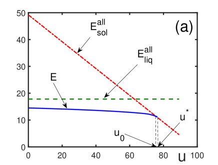
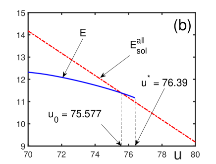
Figure 1. The energy $E$ of a superfluid solid, as compared with the energy $E_{sol}^{all}$ of a pure crystalline state and the energy $E_{liq}^{all}$ of the pure liquid-like phase, as functions of the potential well depth at a lattice site $u$. The right-hand-side figure (b) shows in a larger scale the region of intersection of $E$ and $E_{sol}^{all}$.

Figure 1 shows that the superfluid solid can exist only for $u<75.577$. When the parameter $u$ increases from small values to $u_{0}=75.577$, at this point there happens a first-order quantum phase transition from a superfluid solid to the usual solid. The superfluid solid can exist as a metastable system between $u_{0}=75.577$ and $u=76.39$.

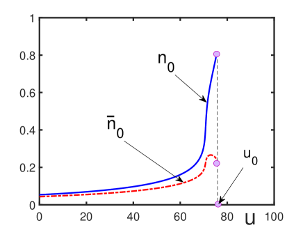
Figure 2. The condensate fraction $n_{0}=N_{0}/N_{liq}$ with respect to the number of particles in the liquid-like phase and the condensate fraction $\overline{n}_{0}=N_{0}/N$ with respect to the total number of particles in the system, as functions of $u$.

Figure 2 presents the condensate fraction $n_{0}=N_{0}/N_{liq}$ normalized to the number of particles in the liquid state and the condensate fraction $\overline{n}_{0}=N_{0}/N$ normalized to the total number of particles in the sample. The relation between these fractions is $\overline{n}_{0}=(1-w)n_{0}$.

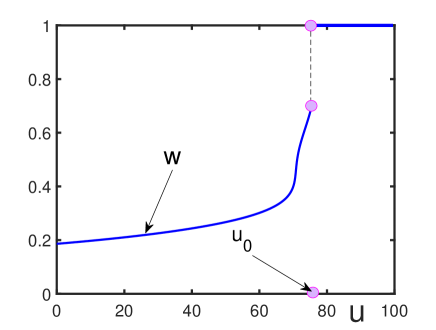
Figure 3. The probability of the solid state $w$ as a function of $u$. For $u>u_{0}$, only the pure solid state can exist.

The behavior of the solid-state probability $w$ is illustrated in Fig. 3. At the point $u_{0}=75.577$, the probability jumps to one and then only the usual solid can exist, while no superfluidity can happen.

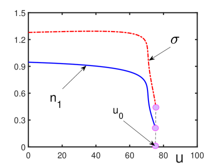
Figure 4. The dimensionless anomalous average $\sigma$ and the fraction of uncondensed particles in the liquid-like phase $n_{1}$, as functions of $u$.

In Fig. 4, the normal average $n_{1}$ and the anomalous average $\sigma$ are shown. The normal average represents the fraction $n_{1}=N_{1}/N_{liq}$ of uncondensed particles in the liquid phase. The modulus of the anomalous average $|\sigma|$ describes the fraction of pair-correlated particles in the liquid-like phase. As is seen, the anomalous average is always larger than the normal average, hence it cannot be neglected.

These results demonstrate that, in general, there exist parameters, where a crystalline solid with regions of disorder, such as dislocations, can exhibit superfluid properties. However for the parameters of hcp ⁴He, this model does not show the existence of superfluidity.

It is necessary to keep in mind that the considered model gives the upper boundary for the possible condensate fractions $n_{0}=N_{0}/N_{liq}$ and, respectively, for $\overline{n}_{0}=N_{0}/N$, with the sole constraint $\overline{n}_{0}<n_{0}$. This is because, for simplicity, in the derivation of the model in the second section, the admissible fraction of the co-existing liquid-like phase $n_{liq}$ was assumed to be allowed for taking the values in the interval $[0,1]$. This, however, is a too wide range of allowed variation of $n_{liq}=N_{liq}/N$, since $n_{liq}$, in reality, is limited by the total possible fraction of particles in the regions of disorder. If, for concreteness, we consider dislocations representing the regions of disorder in solid hcp ⁴He, then we have to take into account the following limitation [20]. The density of dislocations in hcp ⁴He is $10^{4}-10^{6}$ cm^-2, dislocation core radius is of order $10^{-7}$ cm, and dislocation spacing is $10^{-2}$ cm. Then the fraction of particles inside dislocations, with respect to the total number of particles, is of order $10^{-10}-10^{-8}$. Taking this into account, if the upper boundary of the condensate fraction in a solid is $\overline{n}_{0}=N_{0}/N$, then the realistic possible fraction of condensed particles in that solid is not more than $\overline{n}_{0}10^{-8}$. Respectively, if the upper boundary for a fraction is zero, the actual fraction is for sure zero.

4 Conclusion

We have developed a statistical model of a quantum crystal that can house regions of disorder exhibiting liquid-like properties. Examples of such regions of disorder are dislocation networks and grain boundaries. The regions of disorder are randomly distributed inside the sample, which requires to accomplish averaging over phase configurations. As a result of the averaging, we derive a renormalized Hamiltonian describing a crystal with regions of disorder. In the case of Bose particles, in the liquid-like regions there can arise Bose-Einstein condensate, hence there can appear superfluidity. The model allows for the direct evaluation of the probability and fraction of possible Bose condensate, which, of course, depends on the system parameters. For the parameters, characterizing solid hcp helium, the model does not predict the existence of Bose condensate, although, in general, there is a range of parameters, where Bose-condensation and superfluidity inside the regions of disorder in quantum crystals could arise.

Generally, the theory is developed for any temperature. At finite temperatures, we need to consider the thermodynamic potential (30) that has the form $\Omega=\Omega_{sol}+\Omega_{liq}$, where $\Omega_{f}$ are expressed through the renormalized Hamiltonians $H_{f}(w_{f})$ defined in Eq. (29). The thermodynamic potential $\Omega_{sol}$ can be easily calculated in the self-consistent harmonic approximation [55, 56, 57, 58] and the thermodynamic potential $\Omega_{liq}$ can be found in the self-consistent Hartree-Fock-Bogolubov approximation [60, 61, 62, 63, 64].

In the main part of the paper, we concentrate on zero temperature because, first of all, it is exactly at zero temperature where superfluidity, if any, can arise most probably and because presenting the general cumbersome formulas would essentially enlarge the length of the article surpassing the reasonable for a letter limit.

Since the main points of the theory are general, this approach can be applied to systems with different interaction potentials, for instance with dipolar forces. Different interaction potentials will lead to different values of the Debye temperature $T_{D}$, the depth of the potential well $u_{0}$, and the effective interaction strength $\Phi_{0}$. Respectively, depending on the system characteristics, superfluidity in the regions of disorder will either exist or not.

CRediT authorship contribution statement

V.I. Yukalov: Formal analysis, Methodology, Investigation, Writing – original draft, Visualization, Validation. E.P. Yukalova: Formal analysis, Investigation, Writing – original draft, Visualization, Validation, Numerical calculations.

Declaration of competing interest

The authors declare that they have no known competing financial interests or personal relationships that could have appeared to influence the work reported in this paper.

Acknowledgements

This research did not receive any specific grant from funding agencies in the public, commercial, or not-for-profit sectors.

Figure Captions

Figure 1. The energy $E$ of a superfluid solid, as compared with the energy $E_{sol}^{all}$ of a pure crystalline state and the energy $E_{liq}^{all}$ of the pure liquid-like phase, as functions of the potential well depth at a lattice site $u$. The right-hand-side figure (b) shows in a larger scale the region of intersection of $E$ and $E_{sol}^{all}$.

Figure 2. The condensate fraction $n_{0}=N_{0}/N_{liq}$ with respect to the number of particles in the liquid-like phase and the condensate fraction $\overline{n}_{0}=N_{0}/N$ with respect to the total number of particles in the system, as functions of $u$.

Figure 3. The probability of the solid state $w$ as a function of $u$. For $u>u_{0}$, only the pure solid state can exist.

Figure 4. The dimensionless anomalous average $\sigma$ and the fraction of uncondensed particles in the liquid-like phase $n_{1}$, as functions of $u$.

References

- [1] F. Bötcher, J.N. Schmidt, M. Wenzel, J. Hertkorn, M. Guo, T. Langen, T. Pfau, Transient supersolid properties in an array of dipolar quantum droplets, Phys. Rev. X 9 (2019) 011051.
- [2] L. Chomaz, D. Petter, P. Ilzhöfer, G. Natale, A. Trautmann, C. Politi, G. Durastante, R.M. Van Bijnen, A. Patscheider, M. Sohmen, et al. Long-lived and transient supersolid behaviors in dipolar quantum gases, Phys. Rev. X 9 (2019) 021012.
- [3] L. Tanzi, S.M. Roccuzzo, E. Lucioni, F. Fama, A. Fioretti, C. Gabbanini, G. Modugno, A. Recatti, S. Stringari, Supersolid symmetry breaking from compressional oscillations in a dipolar quantum gas, Nature 574 (2019) 382–385.
- [4] M. Guo, F. Böttcher, J. Herkorn, J.N. Schmidt, M. Wenzel, H.P. Bichler, T. Langer, T. Pfau, The low-energy Goldstone mode in a trapped dipolar supersolid, Nature 574 (2019) 386–389.
- [5] F. Böttcher, J.N. Schmidt, J. Hertkorn, K.S.H. Ng, S.D. Graham, M. Guo, T. Langen, T. Pfau, New states of matter with fine-tuned interactions: Quantum droplets and dipolar supersolids, Rep. Prog. Phys. 84 (2021) 012403.
- [6] Z.K. Lu, Y. Li, D.S. Petrov, G.V. Shlyapnikov, Stable dilute supersolid of two-dimensional dipolar bosons, Phys. Rev. Lett. 115 (2015) 075303.
- [7] L.E. Young, S.K. Adhikari, Supersolid-like square- and honeycomb-lattice crystallization of droplets in a dipolar condensate, Phys. Rev. A 105 (2022) 033311.
- [8] S.K. Adhikari, Multiring, stripe, and superlattice solitons in a spin-orbit-coupled spin-1 condensate, Phys. Rev. A 103 (2021) 011301.
- [9] P. Kaur, S. Gautam, S.K. Adhikari, Supersolid-like solitons in a spin-orbit-coupled spin-2 condensate, Phys. Rev. A 105 (2022) 023303.
- [10] N. Prokof’ev, What makes a crystal supersolid? Adv. Phys. 56 (2007) 381–402.
- [11] M. Boninsegni, N.V. Prokof’ev, Supersolids: What and where are they? Rev. Mod. Phys. 84 (2012) 759–776.
- [12] M.H.W. Chan, R.B. Hallock, L. Reatto, Overview on solid 4He and the issue of supersolidity, J. Low Temp. Phys. 172 (2013) 317–363.
- [13] R. Hallock, Is solid helium a supersolid? Phys. Today 68 (2015) 30–35.
- [14] A.B. Kuklov, N.V. Prokof’ev, B.V. Svistunov, Disorder-induced quantum properties of solid 4He, Low Temp. Phys. 46 (2020) 459–464.
- [15] V.I. Yukalov, Saga of superfluid solids, Physics 2 (2020) 45–66.
- [16] D.V. Fil, S.I. Shevchenko, Supersolid induced by dislocations with superfluid cores, Low Temp. Phys. 48 (2022) 429–452.
- [17] O. Penrose, L. Onsager, Bose-Einstein condensation in liquid helium, Phys. Rev. 104 (1956) 576–584.
- [18] J.P. Hirth, J. Lothe, Theory of Dislocations, Wiley, New York, 1982.
- [19] D. Hull, D. Bacon, Introduction to Dislocations, Elsevier, Oxford, 2001.
- [20] F. Souris, A.D. Fefferman, A. Haziot, N. Garroum, J.R. Beamish, S. Balibar, Search for dislocation free Helium crystals, J. Low Temp. Phys. 178 (2014) 149–161.
- [21] S.I. Shevchenko, On quasi-one-dimensional superfluidity in Bose systems, Low Temp. Phys. 14 (1988) 1011–1027.
- [22] D.V. Fil, S.I. Shevchenko, Relaxation of superflow in a network: Application to the dislocation model of supersolidity of helium crystals, Phys. Rev. B 80 (2009) 100501.
- [23] N.N. Bogolubov, Lectures on Quantum Statistics, Ryadyanska Shkola, Kiev, 1949.
- [24] N.N. Bogolubov, Quantum Statistical Mechanics, World Scientific, Singapore, 2015.
- [25] E.P. Gross, Periodic ground states in the many-body problem, Phys. Rev. Lett. 4 (1960) 599–601.
- [26] A. Griesmaier, Generation of a dipolar Bose-Einstein condensate, J. Phys. B 40 (2007) R91.
- [27] M.A. Baranov, Theoretical progress in many-body physics with ultracold dipolar gases, Phys. Rep. 464 (2008) 71–111.
- [28] M. Ueda, Fundamentals and New Frontiers of Bose-Einstein Condensation, World Scientific, Singapore, 2010.
- [29] M.A. Baranov, M. Dalmonte, G. Pupillo, P. Zoller, Condensed matter theory of dipolar quantum gases, Chem. Rev. 112 (2012) 5012–5061.
- [30] D.M. Stamper-Kurn, M. Ueda, Spinor Bose gases: Symmetries, magnetism, and quantum dynamics, Rev. Mod. Phys. 85 (2013) 1191–1244.
- [31] B. Gadway, B. Yan, Strongly interacting ultracold polar molecules, J. Phys. B 49 (2016) 152002.
- [32] V.I. Yukalov, Dipolar and spinor bosonic systems, Laser Phys. 28 (2018) 053001.
- [33] V.I. Yukalov, Remarks on quasiaverages, Theor. Math. Phys. 26 (1976) 274–281.
- [34] V.I. Yukalov, Model of a hybrid crystal, Theor. Math. Phys. 28 (1976) 652–660.
- [35] V.I. Yukalov, Quantum crystal with jumps of particles, Physica A 89 (1977) 363–372.
- [36] V.I. Yukalov, A method to consider metastable states, Phys. Lett. A 81 (1981) 433–435.
- [37] V.I. Yukalov, Theory of melting and crystallization, Phys. Rev. B 32 (1985) 436–446.
- [38] V.I. Yukalov, Phase transitions and heterophase fluctuations, Phys. Rep. 208 (1991) 395–489.
- [39] V.I. Yukalov, Mesoscopic phase fluctuations: General phenomenon in condensed matter, Int. J. Mod. Phys. B 17 (2003) 2333–2358.
- [40] J.W. Gibbs, Collected Works, Yale University, New Haven, 1948.
- [41] N. Bourbaki, Théorie des Ensembles, Hermann, Paris, 1958.
- [42] D. Ruelle, Statistical Mechanics, Benjamin, New York, 1969.
- [43] G.G. Emch, Algebraic Methods in Statistical Mechanics and Quantum Field Theory, Wiley, New York, 1972.
- [44] O. Bratteli, D. Robinson, Operator Algebras and Quantum Statistical Mechanics, Springer, New York, 1979.
- [45] R. Brout, Phase Transitions, Benjamin, New York, 1965.
- [46] S. Kullback, R.A. Leibler, On information and sufficiency, Ann. Math. Stat. 22 (1951) 79–86.
- [47] S. Kullback, Information Theory and Statistics, Wiley, New York, 1959.
- [48] V.I. Yukalov, Effective Hamiltonians for systems with mixed symmetry, Physica A 136 (1986) 575–587.
- [49] V.I. Yukalov, Renormalization of quasi-Hamiltonians under heterophase averaging, Phys. Lett. A 125 (1987) 95–100.
- [50] V.I. Yukalov, Procedure of quasi-averaging for heterophase mixtures, Physica A 141 (1987) 352–374.
- [51] V.I. Yukalov, Lattice mixtures of fluctuating phases, Physica A 144 (1987) 369–389.
- [52] Oxford Living Dictionaries, Oxford University Press, Oxford, 2018.
- [53] J.G. Kirkwood, Quantum Statistics and Cooperative Phenomena, Gordon and Breach, New York, 1965.
- [54] V.I. Yukalov, Statistical systems with nonintegrable interaction potentials, Phys. Rev. E 94 (2016) 012106.
- [55] R.A. Guyer, The physics of quantum crystals, Solid State Phys. 23 (1969) 413–499.
- [56] V.I. Yukalov, V.I. Zubov, Localized-particles approach for classical and quantum crystals, Fortschr. Phys. 31 (1983) 627–672.
- [57] V.I. Yukalov, K. Ziegler, Instability of insulating states in optical lattices due to collective phonon excitations, Phys. Rev. A 91 (2015) 023628.
- [58] V.I. Yukalov, Destiny of optical lattices with strong intersite interactions, Laser Phys. 30 (2020) 015501.
- [59] N. Marzari, A.A. Mostofi, J.R. Yates, I. Souza, D. Vanderbilt, Maximally localized Wannier functions: Theory and applications, Rev. Mod. Phys. 84 (2012) 1419–1476.
- [60] V.I. Yukalov, Fluctuations of composite observables and stability of statistical systems, Phys. Rev. E 72 (2005) 066119.
- [61] V.I. Yukalov, Self-consistent theory of Bose-condensed systems, Phys. Lett. A 359 (2006) 712–717.
- [62] V.I. Yukalov, E.P. Yukalova, Condensate and superfluid fractions for varying interactions and temperature, Phys. Rev. A 76 (2007) 013602.
- [63] V.I. Yukalov, Representative statistical ensembles for Bose systems with broken gauge symmetry, Ann. Phys. (N.Y.) 323 (2008) 461–499.
- [64] V.I. Yukalov and E.P. Yukalova, Ground state of a homogeneous Bose gas of hard spheres, Phys. Rev. A 90 (2014) 013627.
- [65] R.A. Aziz, V.P.S. Nain, J.S. Carley, An accurate intermolecular potential for helium, J. Chem. Phys. 70 (1979) 4330–4342.
- [66] J.A. Hodgdon, F.H. Stillinger, Inherent structures in the potential energy landscape of solid 4He, J. Chem. Phys. 102 (1995) 457–464.
- [67] D.M. Ceperley, R.O. Simmons, R.C. Blasdell, Kinetic energy of liquid and solid 4He, Phys. Rev. Lett. 77 (1996) 115–118.
- [68] S.O. Diallo, J.V. Pearce, R.T. Azuah, H.R. Glyde, Quantum momentum distribution and kinetic energy in solid 4He, Phys. Rev. Lett. 93 (2004) 075301.
- [69] H.J. Maris, S. Balibar, Supersolidity and the thermodynamics of solid Helium, J. Low Temp. Phys. 147 (2007) 539–547.
- [70] C. Cazorla, G.E. Astrakharchik, J. Casulleras, J. Boronat, Bose-Einstein quantum statistics and the ground state of solid 4He, New J. Phys. 11 (2009) 013047.
- [71] S.A. Vitiello, Helium atoms kinetic energy at temperature , J. Low Temp. Phys. 162 (2011) 154–159.
- [72] M.H.W. Chan, Recent experimental studies on solid 4He, J. Low Temp. Phys. 205 (2021) 235–252.
- [73] C. Casorla, J. Boronat, Simulation and understanding of atomic and molecular quantum crystals, Rev. Mod. Phys. 89 (2017) 035003.