Light-induced shear phonon splitting and instability in bilayer graphene

Abstract

Coherent engineering of landscape potential in crystalline materials is a rapidly evolving research field. Ultrafast optical pulses can manipulate low-frequency shear phonons in van der Waals layered materials through the dynamical dressing of electronic structure and photoexcited carrier density. In this work, we provide a diagrammatic formalism for nonlinear Raman force and implement it to shear phonon dynamics in bilayer graphene. We predict a controllable splitting of double degenerate shear phonon modes due to light-induced phonon mixing and renormalization according to a coherent nonlinear Raman force mechanism. Intriguingly, we obtain a light-induced shear phonon softening that facilitates structural instability at a critical field amplitude for which the shear phonon frequency vanishes. The phonon splitting and instability strongly depend on the laser intensity, frequency, chemical potential, and temperature of photoexcited electrons. This study motivates future experimental investigation of the optical fine-tuning and regulation of shear phonons and layer stacking order in layered van der Waals materials.

I Introduction

Exotic emergent phenomena in quantum systems can be generated via photoexcitation by ultrafast optical drives Ishioka et al. (2008); Murakami et al. (2015); Hohenberg and Halperin (1977); Dolgirev et al. (2020); Sun and Millis (2020). Depending on the intensity of the pump laser, we can excite and disentangle collective modes, switch the macroscopic phase of the system, dynamically engineer critical phenomena, and render robust nonlinear couplings among the different degrees of freedom in the quantum materials Huber et al. (2014); Giorgianni et al. (2019); de la Torre et al. (2021). Optical switching and photoinduced transitions correspond to the dynamical modification of the free energy landscape that is not accessible in thermal equilibrium. Photoinduced non-thermal and coherent control of correlated and topological quantum materials Vaswani et al. (2020) is being under investigation in multiple ways, such as Floquet-Bloch dressed single-particle states Oka and Aoki (2009) and optical dressing of many-body interaction couplings Itin and Katsnelson (2015); Aoki et al. (2014). Manipulating and fine-tuning the structural phase of quantum materials by ultrashort laser pulses open a pathway to regulate quantum devices. For instance, substantial lattice deformations are reported induced by intense mid-infrared optical pulse irradiation, e.g., dynamically generated ferroelectricity and shear strain Lejman et al. (2014); Nova et al. (2019). Large photoinduced deformations are due to resonance with a vibration mode, strong Raman force, and nonlinear phonon couplings Lejman et al. (2014); Nova et al. (2019); Horstmann et al. (2020); Disa et al. (2021); de la Torre et al. (2021); Henstridge et al. (2022).

Shear phonons in bilayer and multi-layer of 2D materials, such as the family of graphene, transition metal dichalcogenides (TMDs) and hexagonal Boron Nitride (hBN), correspond to the lateral sliding of atomic layers on each otherTan et al. (2012); Ferrari and Basko (2013); Zhang et al. (2013); Zeng et al. (2012); Michel and Verberck (2008, 2012); Zhao et al. (2013); Wang et al. (2017); Pizzi et al. (2021). Shear phonon excitation can coherently alter the staking order of layers Zhang et al. (2019); Ji et al. (2021), and the electronic topology Sie et al. (2019). Light-induced displacive dynamics Born et al. (1955); Lanzani et al. (2007); Dekorsy et al. (2000); Hase et al. (2003); Ishioka et al. (2006); Zeiger et al. (1992); Pfeifer et al. (1992); Kuznetsov and Stanton (1994, 1995); Stevens et al. (2002); Garrett et al. (1996); Merlin (1997) of coherent shear phonons in van der Waals (vdW) layered materials such as multilayer graphene, WTe₂, and MoTe₂ Zhang et al. (2020); Sie et al. (2019); Zhang et al. (2019); Soranzio et al. (2019); Fukuda et al. (2020); Hein et al. (2020); Ji et al. (2021) is a promising nondestructive mechanism for controlling 2D materials properties. The shear mode in bilayer graphene is a double degenerate Raman-active optical mode and it has a low-frequency $\hbar\Omega_{0}\approx 3.9$meV due to the weak vdW interlayer force Tan et al. (2012). The energy and the intensity of the Raman peak for the shear mode (the C peak) strongly depend on the number of layers and inter-layer coupling. Accordingly, the spectroscopy of interlayer Raman modes is an effective method for determining layer numbers and stacking configurations, and it provides a unique opportunity to explore interlayer couplings. Driving coherent shear phonon in MoTe₂ causes a first-order phase transition from an inversion symmetric 1T^′ structure to the non-centrosymmetric 1T_d phase Zhang et al. (2019); Fukuda et al. (2020). Time and angle-resolved photoemission spectroscopy (tr-ARPES) of the Weyl semimetal T_d-WTe₂, indicates coherent shear phonon-mediated control of the electronic structure Hein et al. (2020). An optical switching from an ABA to ABC stacking is experimentally obtained by laser irradiation on trilayer graphene Zhang et al. (2020) that might be because of the coherent shear phonon excitation.

This paper studies the dynamical engineering of lattice potential for the shear dynamics in vdW layered materials caused by a linear polarised light field ${\bf E}(t)$. The impact of second and third-order Raman susceptibilities gives rise to light-induced corrections to the lattice potential:

$$U=\frac{1}{2}\sum_{\alpha\beta}[\Omega^{2}_{0}\delta_{\alpha\beta}-{\cal G}_{\alpha\beta}({\bf E})]Q_{\alpha}Q_{\beta}-\sum_{\alpha}{\cal F}^{(2)}_{\alpha}({\bf E})Q_{\alpha},$$ (1)

where ${\bf Q}=(Q_{x},Q_{y})$ is the shear phonon displacement with $\Omega_{0}$ being the unperturbed phonon frequency. Displacive Raman shear force described as a second-order effect $\mathbfcal{F}^{(2)}\propto EE^{\ast}$ in bilayer graphene has been previously investigated Rostami (2022). Here, we define the third-order Raman shear force as $\mathbfcal{F}^{(3)}=\overset{\leftrightarrow}{\mathbfcal{G}}\cdot{\bf Q}\propto QEE^{\ast}$ which can renormalize shear phonons and lead to a mode splitting. In particular, it can cause the instability of atomic layers to slide and form stable or metastable phases with different layer-stacking orders due to the softening of shear phonon frequency under the influence of the light field. The ${\cal G}_{\alpha\beta}$ coupling can be interpreted as a light-induced self-energy correction $\Sigma_{\alpha\beta}({\bf E})=-{\cal G}_{\alpha\beta}({\bf E})/2\Omega_{0}$ to the phonon’s dynamical matrix. As the central result, here, we develop a diagrammatic formalism to model the impact of third-order Raman force (or light-induced phonon self-energy) on the displacive dynamics of shear phonons in layered materials. We obtain a dynamical renormalization of the shear phonons by incident light intensity leading to the splitting of the double degenerate shear phonons. We predict a lattice instability where the shear phonon frequency vanishes at a critical field amplitude. We show that the field-induced phonon splitting and instability are highly tunable by the incident laser intensity, frequency at given electronic doping, and temperature. Our theoretical model based on the non-equilibrium Green’s function can be systematically employed in ab initio computations to study the optical engineering of shear phonon in layered materials.

The rest of the paper is structured in four sections. In Section II, we provide details of the diagrammatic method for the third-order Raman force and develop a perturbative theory for optically dressed phonon’s dynamical matrix. In Section III, we summarize the mixed couplings of electrons, phonons, and photons in addition to light-matter and electron-phonon couplings in bilayer graphene. In Section IV, we discuss numerical results for the light-induced phonon renormalization and, thus, its effect on the optical modulation of the shear phonon spectral function, shear mode splitting, and the light-induced shear instability. Finally, we summarize our theoretical finding, discuss it in connection with experiments, and highlight the implication of light-induced phonon renormalization in other heterostructures of 2D materials.

II Method

Stimulated Raman effect is an efficient mechanism to excite Raman-active vibrational modes Dresselhaus et al. (2007). The dipole moment of Raman-active phonon is linearly proportional to the light field $\mu_{b}=\alpha_{bc}E_{c}$ where the polarizability tensor $\alpha_{bc}$ depends on the phonon displacement vector ${\bf Q}$. The electromagnetic potential energy thus follows $U=-\mu_{b}E_{b}=-\alpha_{bc}E_{b}E_{c}$. The corresponding Raman force driving atoms to oscillate follows a second-order nonlinear process Dresselhaus et al. (2007)

$${\cal F}^{(2)}_{a}=-\left[\frac{\partial U}{\partial Q_{a}}\right]_{Q\to 0}=\sum_{bc}\left[\frac{\partial\alpha_{bc}}{\partial Q_{a}}\right]_{Q\to 0}E_{b}E_{c}.$$ (2)

Therefore the lowest-order Raman force is finite as long as the Raman susceptibility is non-vanishing, i.e., $\sigma^{(2)}_{abc}=\partial\alpha_{bc}/\partial Q_{a}\neq 0$. For large displacement, the higher-order Raman force should also be considered, which can dramatically impact phonon renormalization and lattice dynamics. The leading higher-order Raman force depends linearly on the phonon displacement and quadratically on the light field. Therefore, it is described by a third-order nonlinear mechanism

$${\cal F}^{(3)}_{a}=\sum_{bcd}\left[\frac{\partial^{2}\alpha_{cd}}{\partial Q_{a}\partial Q_{b}}\right]_{Q\to 0}Q_{b}E_{c}E_{d}.$$ (3)

Formally, we have ${\cal F}^{(3)}_{a}={\cal G}_{ab}Q_{b}$ in which ${\cal G}_{ab}$ generates a phonon self-energy in terms of a third-order Raman susceptibility $\sigma^{(3)}_{abcd}=\partial^{2}\alpha_{cd}/\partial Q_{a}\partial Q_{b}$ and the incident light intensity. An anisotropic ${\cal G}_{ab}$ breaks the degeneracy of Cartesian shear modes and renormalizes the phonon’s frequency and linewidth.

To model coherent shear phonons in bilayer systems, we first provide a general theory for the Raman force and phonon self-energy using the Green’s function method and diagrammatic framework. We decompose the total Hamiltonian of the system in different parts ${\cal H}={\cal H}_{e}+{\cal H}_{p}+{\cal H}_{e-p}+{\cal H}_{lm}$ which consists of electronic kinetic Hamiltonian ${\cal H}_{e}$, harmonic phonon Hamiltonian ${\cal H}_{p}$, electron-phonon interaction ${\cal H}_{ep}$ and finally the light-matter interaction ${\cal H}_{lm}$. The electronic kinetic Hamiltonian reads $\hat{\cal H}_{e}=\sum_{\bf p}\hat{\psi}^{\dagger}_{\bf p}\hat{\cal H}({\bf p})\hat{\psi}_{\bf p}$ where $\hat{\psi}_{\bf p}$ is the fermion annihilation spinor field at momentum $\bf p$. The harmonic shear phonon Hamiltonian with zero momentum $\bf q=0$ can be written in terms of ladder operators $\hat{\cal H}_{p}=\sum_{\lambda}\hbar\Omega_{0}\hat{b}^{\dagger}_{\lambda}\hat{b}_{\lambda}$ where $\hat{b}_{\lambda}$ is the phonon annihilation operator. We only consider the zone center phonon modes with a vanishing wave vector ${\bf q=0}$, and thus the phonon displacement vector is defined as

$$\hat{Q}_{\lambda}=\sqrt{\frac{\hbar}{\rho S\Omega_{0}}}(\hat{b}_{\lambda}+\hat{b}^{\dagger}_{\lambda})$$ (4)

in which $\lambda=x,y$ indicates two Cartesian mode components, note that $S$ stands for the area of 2D material, and $\rho$ is the mass density. Including both one-phonon and two-phonon couplings to electrons, the electron-phonon interaction Hamiltonian follows

$$\hat{\cal H}_{e-p} =\sum_{\bf p}\sum_{a}\hat{\psi}^{\dagger}_{\bf p}\hat{\cal M}^{(1)}_{a}({\bf p})\hat{\psi}_{\bf p}\hat{Q}_{a}$$

$$+\sum_{\bf p}\sum_{ab}\hat{\psi}^{\dagger}_{\bf p}\hat{\cal M}^{(2)}_{ab}({\bf p})\hat{\psi}_{\bf p}\hat{Q}_{a}\hat{Q}_{b}.$$ (5)

Note that $\hat{\cal M}^{(1)}_{a}$ and $\hat{\cal M}^{(2)}_{ab}$ stand for the one- and two-phonon-electron couplings’ matrix elements, respectively. Utilizing this effective lattice potential and the Heisenberg equation of motion, we obtain the equation of motion for coherent phonon displacement amplitude $Q_{a}$:

$$\frac{\partial^{2}Q_{a}(t)}{\partial t^{2}}+\Gamma_{p}\frac{\partial Q_{a}(t)}{\partial t}+\Omega^{2}_{0}Q_{a}(t)=\frac{{\cal F}_{a}(t)}{\rho}$$

$$+\frac{1}{\rho}\sum_{b}{\cal G}^{ins.}_{ab}(t)Q_{b}(t)+\frac{1}{\rho}\sum_{b}\int dt^{\prime}{\cal G}^{ret.}_{ab}(t,t^{\prime})Q_{b}(t^{\prime})$$ (6)

where $\Omega_{0}$ is the shear phonons frequency, $\Gamma_{p}$ stands for the phenomenological damping frequency of phonons. The leading-order Raman force is given as the expectation value of the one-phonon coupling to electrons:

$${\cal F}^{(2)}_{a}(t)=-\frac{1}{S}\sum_{\bf p}\Big{\langle}\hat{\psi}^{\dagger}_{\bf p}\hat{\cal M}^{(1)}_{a}({\bf p})\hat{\psi}_{\bf p}\Big{\rangle}\Big{|}_{\bf Q\to 0}.$$ (7)

The nonlinear force reveals two different dynamical forms of the light-induced phonon self-energy term ${\cal G}_{ab}$ that we label as instantaneous ${\cal G}^{ins.}_{ab}(t)$ and retarded ${\cal G}^{ret.}_{ab}(t,t^{\prime})$ couplings. The instantaneous coupling is obtained as the expectation value of the two-phonon coupling matrix element

$${\cal G}^{ins.}_{ab}(t)=-\frac{1}{S}\left[\sum_{\bf p}\left\langle\hat{\psi}^{\dagger}_{\bf p}\hat{\cal M}^{(2)}_{ab}({\bf p})\hat{\psi}_{\bf p}\right\rangle\right]_{\bf Q\to 0}.$$ (8)

While the retarded coupling is given by the variational derivative of the Raman force versus the phonon displacement field:

$${\cal G}^{ret.}_{ab}(t,t^{\prime})=-\frac{1}{S}\left[\frac{\delta}{\delta Q_{b}(t^{\prime})}\sum_{\bf p}\Big{\langle}\hat{\psi}^{\dagger}_{\bf p}\hat{\cal M}^{(1)}_{a}({\bf p})\hat{\psi}_{\bf p}\Big{\rangle}\right]_{\bf Q\to 0}.$$ (9)

Note that $\langle\dots\rangle$ indicates quantum statistical averaging. In centrosymmetric systems, Raman-active phonons are infrared-inactive; therefore, they couple to light indirectly. The direct light-matter interaction is only through the coupling to electrons. The coupling of incident light field to electrons can be modeled by Peierls substitution ${\bf p}\to{\bf p}+e{\bf A}(t)$ in the kinetic and the electron-phonon interaction Hamiltonian terms. Considering the homogeneous vector potential ${\bf A}(t)$, the electric field reads ${\bf E}(t)=-\partial_{t}{\bf A}(t)$ and thus ${\bf E}(\omega)=i\omega{\bf A}(\omega)$. Formally, the light-matter interaction Hamiltonian consists of two parts: photon-electron term and photon-electron-phonon term $\hat{\cal H}_{lm}=\hat{\cal H}_{ph-e}+\hat{\cal H}_{ph-e-p}$. The photon-electron term follows

$${\cal H}_{ph-e} =-\sum_{\bf p}\hat{\psi}^{\dagger}_{\bf p}\Big{\{}\sum_{a}\hat{j}_{a}({\bf p})A_{a}(t)$$

$$+\frac{1}{2}\sum_{ab}\hat{\gamma}_{ab}({\bf p})A_{a}(t)A_{b}(t)+\dots\Big{\}}\hat{\psi}_{\bf p}$$ (10)

where $\hat{j}_{a}$ is called the paramagnetic current operator, and $\hat{\gamma}_{ab}$ is known as the diamagnetic current operator as well as the Raman vertex Mahan (1995); Devereaux and Hackl (2007). The photon-electron-phonon interaction Hamiltonian is given by the light field dependence of the electron-phonon interaction, ${\cal M}^{(1)}_{a}({\bf p}+e{\bf A}(t))$ and ${\cal M}^{(2)}_{ab}({\bf p}+e{\bf A}(t))$. By expanding electron-phonon matrix elements up to second-order in ${\bf A}(t)$, we obtain the photon-electron-phonon (PEP) interaction Hamiltonian $\hat{\cal H}_{ph-e-p}=\sum_{\bf p}\hat{\psi}^{\dagger}_{\bf p}\hat{\Xi}_{\bf p}\hat{\psi}_{\bf p}$ where

$$\hat{\Xi}_{\bf p}=\sum_{ab}A_{a}(t)Q_{b}(t)\Big{\{}\hat{\Theta}^{(1)}_{ab}({\bf p})+\sum_{c}\hat{\Theta}^{(2)}_{abc}({\bf p})Q_{c}(t)\Big{\}}$$

$$+\frac{1}{2}\sum_{abc}A_{a}(t)A_{b}(t)Q_{c}(t)\Big{\{}\hat{\Delta}^{(1)}_{abc}({\bf p})+\sum_{d}\hat{\Delta}^{(2)}_{abcd}({\bf p})Q_{d}(t)\Big{\}}.$$ (11)

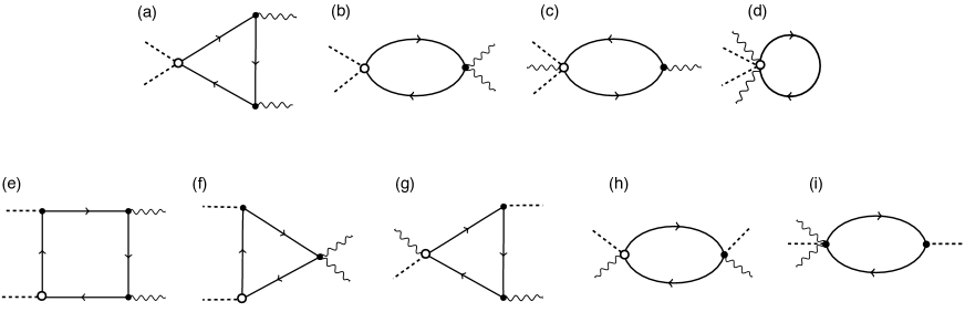
Figure 1: Feynman diagrams for light-induced phonon self-energy. Diagrams given in panel (a-e) and (f-i) for ${\cal G}^{ins.}$ and ${\cal G}^{ret.}$ couplings, respectively. Dashed and wave lines represent external phonon and photon fields, respectively. The solid lines represent electron propagators.

Having defined all vertex couplings, we are equipped to evaluate the Raman force and the light-induced phonon self-energy. Because the Raman phonon is even under parity, the leading contribution to the Raman force is second order in the light field, which follows

$${\cal F}^{(2)}_{a}(t)=\sum_{bc}\sum_{\omega_{1},\omega_{2}}e^{i(\omega_{1}+\omega_{2})t}\sigma^{(2)}_{abc}(\omega_{1},\omega_{2})E_{b}(\omega_{1})E_{c}(\omega_{2}).$$ (12)

Similarly, the light-induced instantaneous coupling is given by

$${\cal G}^{ins.}_{ab}(t)=\sum_{cd}\sum_{\omega_{1},\omega_{2}}e^{i(\omega_{1}+\omega_{2})t}\Pi^{ins.}_{abcd}(\omega_{1},\omega_{2})E_{c}(\omega_{1})E_{d}(\omega_{2}).$$ (13)

Finally, one can evaluate the light-induced retarded coupling as follows

$${\cal G}^{ret.}_{ab}(t,t^{\prime}) =\sum_{cd}\sum_{\omega_{1},\omega_{2}}e^{i(\omega_{1}+\omega_{2})t}\Pi^{ret.}_{abcd}(\omega_{1},\omega_{2},t-t^{\prime})$$

$$\times E_{c}(\omega_{1})E_{d}(\omega_{2}).$$ (14)

Notice that $\Pi^{ret.}_{abcd}(\omega_{1},\omega_{2},\tau)=\sum_{\omega_{3}}e^{i\omega_{3}\tau}\Pi^{ret.}_{abcd}(\omega_{1},\omega_{2},\omega_{3})$ where $\omega_{3}$ is the phonon frequency. Response function $\Pi^{ins.}_{abcd}$ contributes to the instantaneous phonon self-energy since it originates from the simultaneous coupling of two phonons to electrons. On the other hand, the retarded response function $\Pi^{ret.}_{abcd}$ contains memory effects where the past dynamics of phonons can influence their future motion.

The light-induced rigid displacement directly depends on the displacive Raman force that is the rectified part of the force in a second-order nonlinear process Rostami (2022). We consider monochromatic incident light-field ${\bf E}(t)=E_{0}\hat{\bm{\varepsilon}}e^{-i\omega t}+c.c.$ with $\hat{\bm{\varepsilon}}$ being the linear polarization unit vector. The displacive force is thus given by the rectification process (i.e., $\omega_{1}=-\omega_{2}=\omega$) that leads to the following time-independent Raman force:

$${\cal F}^{\rm D}_{a} =\sum_{bc}\sigma^{(2)}_{abc}(\omega,-\omega)E_{b}(\omega)E^{\ast}_{c}(\omega).$$ (15)

Similarly, the rectified component of the instantaneous phonon-phonon coupling reads

$${\cal G}^{ins.}_{ab}=\sum_{cd}\Pi^{ins.}_{abcd}(\omega,-\omega)E_{c}(\omega)E^{\ast}_{d}(\omega),$$ (16)

and the retarded light-induced phonon-phonon coupling follows

$${\cal G}^{ret.}_{ab}(t-t^{\prime})=\sum_{cd}\Pi^{ret.}_{abcd}(\omega,-\omega,t-t^{\prime})E_{c}(\omega)E^{\ast}_{d}(\omega).$$ (17)

It is worth highlighting that the second harmonic parts of ${\cal G}^{ins.}_{ab}$ and ${\cal G}^{ret.}_{ab}$ $\sim e^{i2\omega t}$ do not contribute noticeably due to its convolution with the slow oscillation of the ion displacement $Q_{a}\sim e^{i\Omega_{0}t}$ since $\omega\gg\Omega_{0}$. In this regard, the rectified parts of ${\cal G}^{ins.}_{ab}$ and ${\cal G}^{ret.}_{ab}$ play the dominant role. Eventually, the phonon equation of motion coherently dressed by the light field is given by

$$\frac{\partial^{2}Q_{a}(t)}{\partial t^{2}}+\Gamma_{p}\frac{\partial Q_{a}(t)}{\partial t}+\Omega^{2}_{0}Q_{a}(t)=\frac{{\cal F}^{\rm D}_{a}}{\rho}+\frac{1}{\rho}\sum_{b}{\cal G}^{ins.}_{ab}Q_{b}(t)$$

$$+\frac{1}{\rho}\sum_{b}\int dt^{\prime}{\cal G}^{ret.}_{ab}(t-t^{\prime})Q_{b}(t^{\prime}).$$ (18)

We employ a diagrammatic formalism to estimate numerical values of the Raman force Rostami (2022) and phonon self-energy. Here, the main focus is on the light-induced renormalization and mixing of shear phonons. The Feynman diagrams for the instantaneous and retarded couplings thus are given in Fig. 1a-d and Fig. 1e-i, respectively. To quantitatively analyze the spectral function and the splitting of shear phonons, we microscopically explore the coherent dynamics of shear modes in bilayer graphene in the remaining part of the paper.

III Light-matter and electron-phonon couplings

Bilayer graphene consists of two single layers of graphene sheets offset from each other in the $xy$ plane. The low-energy quasiparticles follow a two-band Hamiltonian around the corners of the hexagonal Brillouin zone McCann and Fal’ko (2006)

$$\hat{H}_{\bf p}=-\frac{1}{2m}\{(p^{2}_{x}-p^{2}_{y})\hat{\sigma}_{x}+2\tau p_{x}p_{y}\hat{\sigma}_{y}\}-\mu\hat{I}.$$ (19)

Note that ${\bm{p}}=\hbar{\bm{k}}$ is the momentum vector, $\tau=\pm$ indicates two K and K^′ valley points, the identity matrix $\hat{I}$ and Pauli matrices $\hat{\sigma}_{x}$ and $\hat{\sigma}_{y}$ are in the layer pseudospin basis, and $\mu$ is the chemical potential. In our convention, the $x$-direction shows a zigzag orientation of the honeycomb lattice Rostami and Asgari (2013). The effective mass is given by $1/2m\approx v^{2}/|\gamma_{1}|$ with $v\approx 10^{6}$m/s and vertical inter-layer hopping energy $\gamma_{1}\approx-0.4$eV McCann and Koshino (2013). Having the in-plane displacement ${\bf Q}^{(\ell)}({\bf r})$ of two layers $\ell=1,2$, the shear phonon displacement is the asymmetric component:

$${\bf Q}=\frac{{\bf Q}^{(1)}-{\bf Q}^{(2)}}{\sqrt{2}}.$$ (20)

The shear displacement vector is even under parity ${\cal P}$ since ${\cal P}\{{\bf Q}^{(1)},{\bf Q}^{(2)}\}{\cal P}^{-1}=-\{{\bf Q}^{(2)},{\bf Q}^{(1)}\}$ leading to ${\cal P}{\bf Q}{\cal P}^{-1}={\bf Q}$. Therefore, the shear mode is a Raman-active but IR-inactive phonon. We consider the coupling of electrons to one and two photons given by $\hat{j}_{\alpha}=-e\partial_{p_{\alpha}}\hat{H}_{\bf p}$ and $\hat{\gamma}_{\alpha\beta}=-e^{2}\partial_{p_{\alpha}}\partial_{p_{\beta}}\hat{H}_{\bf p}$, respectively. The coupling of electrons to one and two photons are thus given by

$$(\hat{j}_{x},\hat{j}_{y})=\frac{e}{m}(p_{x}\hat{\sigma}_{x}+\tau p_{y}\hat{\sigma}_{y},-p_{y}\hat{\sigma}_{x}+\tau p_{x}\sigma_{y}),$$

$$(\hat{\gamma}_{xx}=-\hat{\gamma}_{yy},\hat{\gamma}_{xy}=\hat{\gamma}_{yx})=\frac{e^{2}}{m}(\hat{\sigma}_{x},\tau\hat{\sigma}_{y}).$$ (21)

The electron-phonon couplings are obtained using a four-band tight-binding model following the approach developed in Ref. Rostami (2022) providing the detailed analysis of electron coupling to shear phonons in bilayer graphene using tight-binding and ${\bf k\cdot p}$ models– see also Refs. Ishikawa and Ando (2006); Cappelluti and Profeta (2012); Basko (2009). Accordingly, the couplings of electrons to shear phonons in the low-energy model read Rostami (2022)

$$(\hat{\cal M}^{(1)}_{x},\hat{\cal M}^{(1)}_{y})\approx{\cal M}^{(1)}(\tau\hat{\sigma}_{y},\hat{\sigma}_{x}),$$

$$(\hat{\cal M}^{(2)}_{xx}=-\hat{\cal M}^{(2)}_{yy},\hat{\cal M}^{(2)}_{xy}=\hat{\cal M}^{(2)}_{yx})\approx{\cal M}^{(2)}(\hat{\sigma}_{x},\tau\hat{\sigma}_{y}).$$ (22)

Electron-phonon coupling can depend on the light field, and this leads to mixed PEP couplings which are obtained after neglecting electron momentum $p$ Rostami (2022)

$$\begin{pmatrix}\hat{\Theta}^{(1)}_{xy}=\hat{\Theta}^{(1)}_{yx}\\ \hat{\Theta}^{(1)}_{yy}=-\hat{\Theta}^{(1)}_{xx}\end{pmatrix}\approx-\Theta^{(1)}\begin{pmatrix}\tau\hat{\sigma}_{x}\\ \hat{\sigma}_{y}\end{pmatrix},$$ (23)

$$\begin{pmatrix}\Theta^{(2)}_{yyx}=\Theta^{(2)}_{yxy}=\Theta^{(2)}_{xyy}=\Theta^{(2)}_{xxx}/3\\ \Theta^{(2)}_{xyx}=\Theta^{(2)}_{xxy}=\Theta^{(2)}_{yxx}=\Theta^{(2)}_{yyy}/3\end{pmatrix}\approx\Theta^{(2)}\begin{pmatrix}\tau\hat{\sigma}_{x}\\ -\hat{\sigma}_{y}\end{pmatrix},$$ (24)

$$\begin{pmatrix}\Delta^{(1)}_{xxy}=\Delta^{(1)}_{xyx}=\Delta^{(1)}_{yxx}=\Delta^{(1)}_{yyy}/3\\ \Delta^{(1)}_{yxy}=\Delta^{(1)}_{yyx}=\Delta^{(1)}_{xyy}=\Delta^{(1)}_{xxx}/3\end{pmatrix}\approx\Delta^{(1)}\begin{pmatrix}\hat{\sigma}_{x}\\ \tau\hat{\sigma}_{y}\end{pmatrix}.$$ (25)

The expression for $\Delta^{(2)}_{abcd}$ coupling, representing the coupling of two-photon and two-phonon fields with an electron field, has yet to be specified. However, we can include its contribution using a gauge invariance argument, and therefore there is no need to explicitly calculate $\Delta^{(2)}_{abcd}$ coupling constants. This gauge invariance issue is discussed more explicitly in the following sections.

The values of electron-phonon couplings strength are given in terms of microscopic parameters of the system Rostami (2022)

$${\cal M}^{(1)}=-\Big{(}\frac{3a_{0}}{\sqrt{2}b}\Big{)}\Big{(}\frac{\partial\gamma_{3}}{\partial b}\Big{)}=\Big{(}\frac{3a_{0}\gamma_{3}}{\sqrt{2}b^{2}}\Big{)}\beta_{3},$$ (26)

$${\cal M}^{(2)}=\Big{(}\frac{3a^{2}_{0}}{4b^{2}}\Big{)}\Big{(}\frac{\partial^{2}\gamma_{3}}{\partial b^{2}}\Big{)}=\Big{(}\frac{3a^{2}_{0}\gamma_{3}}{4b^{4}}\Big{)}\beta_{3}(1+\beta_{3}).$$ (27)

where $\gamma_{3}\approx 0.3$eV McCann and Koshino (2013) is an interlayer hopping energy corresponding to the hopping of electrons from sublattice A of bottom layer one to sublattice A of the top layer in a Bernal stack bilayer system. The Gruneisen parameter follows $\beta_{3}=-\partial\ln\gamma_{3}/\partial\ln b$. The mixed PEP coupling constants are thus obtained as $\Theta^{(1)}=({ea_{0}}/{2\hbar}){\cal M}^{(1)}$, $\Delta^{(1)}=({ea_{0}}/{2\hbar})^{2}{\cal M}^{(1)}$ and $\Theta^{(2)}=-({ea_{0}}/{4\hbar}){\cal M}^{(2)}$. Accordingly, the only coupling parameter is $\beta_{3}$. In the second equality of the above relation, we assume the power-law rule $\gamma_{3}\sim 1/b^{\beta_{3}}$ for the dependence of $\gamma_{3}$ on the corresponding bond length $b=\sqrt{a^{2}_{0}+c^{2}}\approx 0.38$nm with intralayer Carbon-Carbon bond length $a_{0}=0.142$nm and the interlayer distance $c=0.34$nm. An analysis based on the density functional calculation estimates the dependence of $\gamma_{3}$ on the bond length as $\partial\gamma_{3}/\partial b\approx-0.54{\rm eV/\AA}$ Cappelluti and Profeta (2012) and therefore one can obtain the Gruneisen parameter $\beta_{3}=-(b/\gamma_{3})\partial\gamma_{3}/\partial b\approx 6.84$. The vertical hopping derivative ${\partial\gamma_{1}}/{\partial c}$ does not contribute to the leading order electron-phonon interaction.

IV Numerical results and discussion

The phonon self-energy terms depend on $\Pi^{ins.}_{abcd}$ and $\Pi^{ret.}_{abcd}$ which are given in terms of corresponding susceptibilities ${\mathchoice{\raisebox{0.0pt}{$\displaystyle\chi$}}{\raisebox{0.0pt}{$\textstyle\chi$}}{\raisebox{0.0pt}{$\scriptstyle\chi$}}{\raisebox{0.0pt}{$\scriptscriptstyle\chi$}}}^{ins.}_{abcd}$ and ${\mathchoice{\raisebox{0.0pt}{$\displaystyle\chi$}}{\raisebox{0.0pt}{$\textstyle\chi$}}{\raisebox{0.0pt}{$\scriptstyle\chi$}}{\raisebox{0.0pt}{$\scriptscriptstyle\chi$}}}^{ret.}_{abcd}$ in response to the vector potentials $A_{c}(\omega_{1})$ and $A_{d}(\omega_{2})$. Therefore, we have

$$\Pi^{ins.}_{abcd}(\omega_{1},\omega_{2})=-\frac{{\mathchoice{\raisebox{0.0pt}{$\displaystyle\chi$}}{\raisebox{0.0pt}{$\textstyle\chi$}}{\raisebox{0.0pt}{$\scriptstyle\chi$}}{\raisebox{0.0pt}{$\scriptscriptstyle\chi$}}}^{ins.}_{abcd}(\omega_{1},\omega_{2})}{(i\omega_{1})(i\omega_{2})},$$ (28)

$$\Pi^{ret.}_{abcd}(\omega_{1},\omega_{2},\omega_{3})=-\frac{{\mathchoice{\raisebox{0.0pt}{$\displaystyle\chi$}}{\raisebox{0.0pt}{$\textstyle\chi$}}{\raisebox{0.0pt}{$\scriptstyle\chi$}}{\raisebox{0.0pt}{$\scriptscriptstyle\chi$}}}^{ret.}_{abcd}(\omega_{1},\omega_{2},\omega_{3})}{(i\omega_{1})(i\omega_{2})}.$$ (29)

where $\omega_{3}$ is the phonon frequency. The overall minus sign in the above relations by definition, given in Eq. (8) and Eq. (9). Utilizing Feynman diagrams given in Fig. 1(a-d) and Fig. 1(e-i) we calculate ${\mathchoice{\raisebox{0.0pt}{$\displaystyle\chi$}}{\raisebox{0.0pt}{$\textstyle\chi$}}{\raisebox{0.0pt}{$\scriptstyle\chi$}}{\raisebox{0.0pt}{$\scriptscriptstyle\chi$}}}^{ins.}_{abcd}$ and ${\mathchoice{\raisebox{0.0pt}{$\displaystyle\chi$}}{\raisebox{0.0pt}{$\textstyle\chi$}}{\raisebox{0.0pt}{$\scriptstyle\chi$}}{\raisebox{0.0pt}{$\scriptscriptstyle\chi$}}}^{ret.}_{abcd}$ response functions, respectively. Before reporting the numerical results, it is necessary to mention that the contribution of the mixed PEP coupling $\Delta^{(2)}_{abcd}$, depicted in the diagram in Fig. 1d, is frequency-independent. One can incorporate this diagram by enforcing the gauge invariance, implying a vanishing system response to a static homogeneous gauge field. Accordingly, we have ${\mathchoice{\raisebox{0.0pt}{$\displaystyle\chi$}}{\raisebox{0.0pt}{$\textstyle\chi$}}{\raisebox{0.0pt}{$\scriptstyle\chi$}}{\raisebox{0.0pt}{$\scriptscriptstyle\chi$}}}^{ins.}_{abcd}(\omega_{1}=0,\omega_{2}=0)+{\mathchoice{\raisebox{0.0pt}{$\displaystyle\chi$}}{\raisebox{0.0pt}{$\textstyle\chi$}}{\raisebox{0.0pt}{$\scriptstyle\chi$}}{\raisebox{0.0pt}{$\scriptscriptstyle\chi$}}}^{ret.}_{abcd}(\omega_{1}=0,\omega_{2}=0,\omega_{3})=0$ so that the impact of $\Delta^{(2)}_{abcd}$ can be taken into account by subtracting the static value of each diagram.

$${\mathchoice{\raisebox{0.0pt}{$\displaystyle\chi$}}{\raisebox{0.0pt}{$\textstyle\chi$}}{\raisebox{0.0pt}{$\scriptstyle\chi$}}{\raisebox{0.0pt}{$\scriptscriptstyle\chi$}}}^{ret.}_{abcd}(\omega_{1},\omega_{2},\omega_{3})\to{\mathchoice{\raisebox{0.0pt}{$\displaystyle\chi$}}{\raisebox{0.0pt}{$\textstyle\chi$}}{\raisebox{0.0pt}{$\scriptstyle\chi$}}{\raisebox{0.0pt}{$\scriptscriptstyle\chi$}}}^{ret.}_{abcd}(\omega_{1},\omega_{2},\omega_{3})-{\mathchoice{\raisebox{0.0pt}{$\displaystyle\chi$}}{\raisebox{0.0pt}{$\textstyle\chi$}}{\raisebox{0.0pt}{$\scriptstyle\chi$}}{\raisebox{0.0pt}{$\scriptscriptstyle\chi$}}}^{ret.}_{abcd}(0,0,\omega_{3}),$$

$${\mathchoice{\raisebox{0.0pt}{$\displaystyle\chi$}}{\raisebox{0.0pt}{$\textstyle\chi$}}{\raisebox{0.0pt}{$\scriptstyle\chi$}}{\raisebox{0.0pt}{$\scriptscriptstyle\chi$}}}^{ins.}_{abcd}(\omega_{1},\omega_{2})\to{\mathchoice{\raisebox{0.0pt}{$\displaystyle\chi$}}{\raisebox{0.0pt}{$\textstyle\chi$}}{\raisebox{0.0pt}{$\scriptstyle\chi$}}{\raisebox{0.0pt}{$\scriptscriptstyle\chi$}}}^{ins.}_{abcd}(\omega_{1},\omega_{2})-{\mathchoice{\raisebox{0.0pt}{$\displaystyle\chi$}}{\raisebox{0.0pt}{$\textstyle\chi$}}{\raisebox{0.0pt}{$\scriptstyle\chi$}}{\raisebox{0.0pt}{$\scriptscriptstyle\chi$}}}^{ins.}_{abcd}(0,0).$$ (30)

The rest of the section summarises our analytical and numerical results for the light-induced instantaneous and retarded couplings and the resulting renormalization of shear phonon frequency in bilayer graphene. Afterward, we quantitatively analyze the splitting of shear phonon modes and phonon instability which are coherently controllable by altering the incident laser intensity, frequency, and polarization. We also investigate the impact of finite electronic temperature on our numerical results.

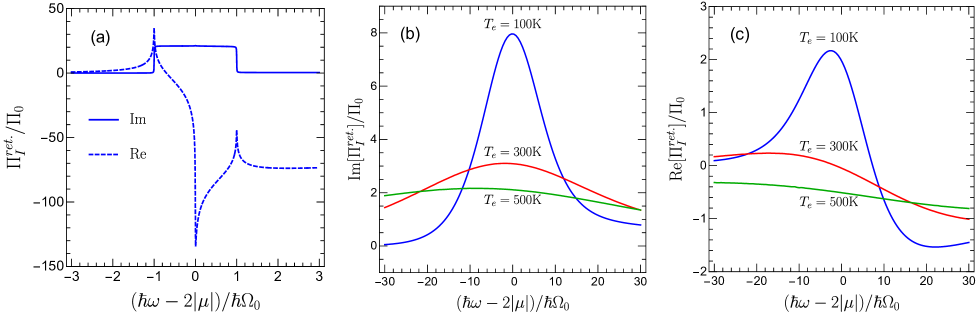
Figure 2: Light-induced retarded self-energy coupling versus the laser frequency. Panel (a) indicates the imaginary and real parts of $\Pi^{ret.}_{I}$ versus the incident laser frequency at zero electronic temperature $T_{e}=0$ and $\Gamma_{e}=0.001$meV. Panel (b) and (c) respectively illustrate the imaginary and real parts of $\Pi^{ret.}_{I}$ at $\Gamma_{e}=1$meV and different values of electronic temperature $T_{e}$. We set $\mu=200$meV, and $\hbar\Omega_{0}=3.9$meV in this figure.

IV.1 Light-induced instantaneous self-energy

Light-induced instantaneous phonon self-energy is calculated following the Feynman diagrams depicted in Fig. 1a-d employing the effective low-energy description of electrons and the couplings to phonons and photons. For a linearly polarized incident light field ${\bf E}(t)=E_{0}(\hat{\bf x}\cos\theta+\hat{\bf y}\sin\theta)e^{-i\omega t}+c.c$, the symmetry of the system enforces the following constraints for the only non-vanishing tensor elements as $-\Pi^{ins.}_{xxxx}=-\Pi^{ins.}_{yyyy}=\Pi^{ins.}_{xxyy}=\Pi^{ins.}_{yyxx}=\Pi^{ins.}_{xyxy}=\Pi^{ins.}_{yxyx}=\Pi^{ins.}_{xyyx}=\Pi^{ins.}_{yxxy}=\Pi^{ins.}$. In accordance with this symmetry constrain, we find the dependence of $\hat{\cal G}^{ins.}$ on the light field polarization angle $\theta$:

$$\hat{\cal G}^{ins.}=\Pi^{ins.}(\bar{\omega}_{1},\bar{\omega}_{2})E^{2}_{0}\begin{bmatrix}-\cos(2\theta)&\sin(2\theta)\\[5.0pt] \sin(2\theta)&\cos(2\theta)\end{bmatrix}$$ (31)

where $\bar{\omega}_{j}=\hbar(\omega_{j}+i\Gamma_{e})/|\mu|$ with $\omega_{1}=-\omega_{2}=\omega$ and $\hbar\Gamma_{e}$ is the electron scattering rate. The functional dependence of the instantaneous coupling is obtained analytically using the effective low-energy Hamiltonian, and it reads $\Pi^{ins.}(\bar{\omega}_{1},\bar{\omega}_{2})={\Pi}^{ins.}_{0}\Lambda(\bar{\omega}_{1},\bar{\omega}_{2})$ with (see Appendix A)

$$\Lambda(\bar{\omega}_{1},\bar{\omega}_{2}) =\Bigg{\{}\frac{(\bar{\omega}_{1}+2\bar{\omega}_{2})}{\bar{\omega}^{2}_{2}(\bar{\omega}_{1}+\bar{\omega}_{2})}\ln\left[\frac{4-\bar{\omega}^{2}_{1}}{4-(\omega_{1}+\omega_{2})^{2}}\right]$$

$$+\frac{(\bar{\omega}_{2}+2\bar{\omega}_{1})}{\bar{\omega}^{2}_{1}(\bar{\omega}_{1}+\bar{\omega}_{2})}\ln\left[\frac{4-\bar{\omega}^{2}_{2}}{4-(\bar{\omega}_{1}+\bar{\omega}_{2})^{2}}\right]$$

$$-\frac{3}{2\bar{\omega}_{1}\bar{\omega}_{2}}\ln\left[1-\frac{(\omega_{1}+\omega_{2})^{2}}{4}\right]\Bigg{\}},$$ (32)

and the dimensionful constant prefactor reads

$${\Pi}^{ins.}_{0}=\frac{N_{f}e^{2}{\cal M}^{(2)}}{4\pi\mu^{2}}.$$ (33)

in which $N_{f}=4$ stands for the spin-valley degeneracy. The properties of universal function $\Lambda(\omega_{1},\omega_{2})$ are explored in Ref. Rostami (2022) at zero and finite electronic temperature $T_{e}$.

IV.2 Light-induced retarded self-energy

For the retarded coupling, we have the Feynman diagrams depicted in Fig. 1(e-i), among which only diagrams shown in panels (e), (h), and (i) of Fig. 1 are non-zero in our effective model analysis. The symmetry of our low-energy model results in constraints for the non-vanishing elements of $\Pi^{ret.}_{abcd}$ as $\Pi^{ret.}_{xxxx}=\Pi^{ret.}_{yyyy}$, $\Pi^{ret.}_{xxyy}=\Pi^{ret.}_{yyxx}$, $\Pi^{ret.}_{xyxy}=\Pi^{ret.}_{yxyx}$ and $\Pi^{ret.}_{xyyx}=\Pi^{ret.}_{yxxy}$. Accordingly, the polarization dependence of the retarded coupling reads

$$\hat{\cal G}^{ret.}(\Omega) =E^{2}_{0}\Pi^{ret.}_{I}\hat{I}+E^{2}_{0}\begin{bmatrix}\Pi^{ret.}_{Z}\cos(2\theta)&\Pi^{ret.}_{X}\sin(2\theta)\\[5.0pt] \Pi^{ret.}_{X}\sin(2\theta)&-\Pi^{ret.}_{Z}\cos(2\theta)\end{bmatrix},$$ (34)

where for a given light field frequency $\omega$ and at phonon frequency $\Omega$, we define

$$\Pi^{ret.}_{I,Z}(\omega,-\omega,\Omega) =\frac{\Pi^{ret.}_{xxxx}\pm\Pi^{ret.}_{xxyy}}{2},$$

$$\Pi^{ret.}_{X}(\omega,-\omega,\Omega) =\frac{\Pi^{ret.}_{xyyx}+\Pi^{ret.}_{xyxy}}{2}.$$ (35)

The $+$ and $-$ signs in the above relation refer to $\Pi^{ret.}_{I}$ and $\Pi^{ret.}_{Z}$, respectively. The three contributions from three diagrams Fig. 2a,d,e can be collected as follows

$$\Pi^{ret.}_{\xi=I,Z,X}(\omega_{1},\omega_{2},\omega_{3})=\Pi^{ret.}_{0}\Big{\{}\Pi^{\rm square}_{\xi}(\omega_{1},\omega_{2},\omega_{3})+$$

$$\alpha\left[\Pi^{\rm bubble-\Theta}_{\xi}(\omega_{1},\omega_{2},\omega_{3})+\Pi^{\rm bubble-\Delta}_{\xi}(\omega_{1},\omega_{2},\omega_{3})\right]\Big{\}}.$$ (36)

In the low-energy model, we obtain vanishing contributions for the triangle diagrams shown in Fig. 1f,g. The detailed derivation and analytical expressions of the above nonlinear response functions at zero electronic temperature are given in Appendix B. Notice the constant factors

$$\Pi^{ret.}_{0} =\frac{N_{f}(e{\cal M}^{(1)})^{2}}{24\pi(\hbar\Gamma_{e})\mu^{2}}~{}~{},~{}~{}\alpha=\frac{\hbar\Gamma_{e}}{(18\gamma^{2}_{0}/\gamma_{1})}.$$ (37)

Since $18\gamma^{2}_{0}/\gamma_{1}\approx 10^{2}$eV and $\hbar\Gamma_{e}$ is usually less than tens of meV, we have $\alpha\ll 1$ for realistic value of scattering rate $\hbar\Gamma_{e}$. Therefore, we safely neglect the contribution of bubble diagrams relative to the square diagram. Considering the square diagram, our microscopic calculation gives $\Pi^{ret.}_{xxxx}=\Pi^{ret.}_{xxyy}$ and $\Pi^{ret.}_{xyxy}=-\Pi^{ret.}_{xyyx}$. Consequently, we obtain

$$\Pi^{ret.}_{I}=\Pi^{ret.}_{xxxx}\approx\Pi^{\rm square}_{I}~{}~{}~{}\text{and}~{}~{}~{}\Pi^{ret.}_{Z}=\Pi^{ret.}_{X}=0.$$ (38)

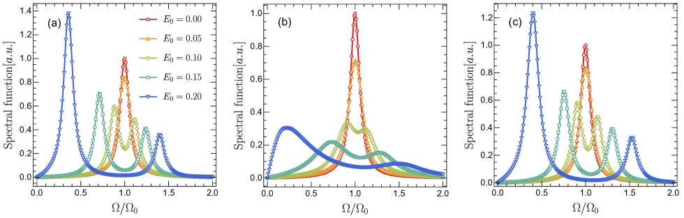
Figure 3: Adiabatic and non-adiabatic spectral functions of optically dressed shear phonons. Panels (a) and (b) illustrate the results obtained within the adiabatic and non-adiabatic models, respectively. In panel (c), we depict the spectral function obtained after neglecting the imaginary part of $\Pi^{ret}_{I}(\Omega)$. The shear phonons’ splitting is depicted at different values of the light field amplitude in the unit of V/nm. The splitting is almost the same in both adiabatic and non-adiabatic models. However, the linewidth and peak values are different in the two models. We set $\mu=200$meV, $\hbar\Gamma_{e}=5$meV, $\hbar\Gamma_{p}=0.5$meV, $T_{e}=100$K, $\hbar\Omega_{0}=3.9$meV and $\theta=0$ in this figure.

In Fig. 2, we illustrate real and imaginary parts of $\Pi^{ret.}_{I}$ at zero and finite electronic temperature $T_{e}$. At very low temperatures, the imaginary part is finite only in a narrow frequency window close to the interband optical transition gap $2|\mu|$ where the width of the frequency window is given by the shear phonon frequency $2\Omega_{0}$. The real part of $\Pi^{ret.}_{I}$ shows logarithmic cusps at optical transition edges for $\hbar\omega=2\mu$ and $\hbar\omega=2\mu\pm\hbar\Omega$.

We generalize the zero temperature response function $\Pi_{abcd}(\varepsilon_{F},T_{e}=0,\dots)$ to finite electronic temperature using the Maldague’s formula Giuliani and Vignale (2005); Rostami (2022), by integrating over the Fermi energy as follows

$$\Pi_{abcd}|_{\mu,T_{e}}=\int^{\infty}_{-\infty}dy\frac{\Pi_{abcd}|_{\varepsilon_{F}\to y,T_{e}=0}}{4k_{B}T_{e}\cosh^{2}\left({\frac{y-\mu}{2k_{B}T_{e}}}\right)}.$$ (39)

The electronic temperature can reach thousands of Kelvin due to intense and ultrashort laser pulses Lui et al. (2010); Tomadin et al. (2013); Brida et al. (2013); Tomadin et al. (2018); Andreatta et al. (2019). The imaginary part of $\Pi^{ret.}_{I}$ is always positive at zero and finite temperatures. We investigate the impact of the electronic temperature, and the result shows an expected reduction of the response for frequencies in the range $|\hbar\omega-2|\mu||<\hbar\Omega_{0}$ while outside this range, the response function increases by raising the temperature.

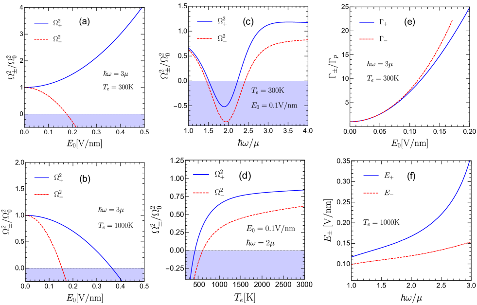
Figure 4: Light-induced shear phonon splitting and instability. Panel (a) and (b) shows the mode splitting as a function of the light field amplitude at laser frequency $\hbar\omega=3\mu$ and two different values of electronic temperature. Panel (c) illustrates the frequency dependence of dynamically renormalized shear modes at field amplitude $E_{0}=0.1$V/nm and $T_{e}=300$K. Panel (d) indicates the shear phonon frequencies versus the electronic temperature at $\hbar\omega=2\mu$ and $E_{0}=0.1$V/nm. Panel (e) shows the field dependence of shear phonon linewidth at $\hbar\omega=3\mu$ and $T_{e}=300$K. Panel (f) manifests the laser frequency dependence of the critical field amplitude at which phonon modes become unstable. We set $\mu=200$meV, $\hbar\Gamma_{p}=0.1$meV, $\hbar\Gamma_{e}=5$meV and $\hbar\Omega_{0}=3.9$meV in this figure.

IV.3 Light-induced phonon splitting and instability

Performing the Fourier transform of the shear phonon displacement vector $Q_{a}(t)=\sum_{\Omega}Q_{a}(\Omega)e^{-i\Omega t}$ in Eq. (II) leads to the equation of motion into the frequency domain

$$\sum_{b}\Big{\{}{\cal K}_{ab}(\Omega)-(\Omega^{2}+i\Gamma_{p}\Omega)\delta_{ab}\Big{\}}Q_{b}(\Omega)=\frac{{\cal F}^{\rm D}_{a}}{\rho}$$ (40)

where the dynamical matrix of shear modes is dressed by the external light field and given by

$${\cal K}_{ab}(\Omega)=\Omega^{2}_{0}\delta_{ab}-\frac{{\cal G}^{ins.}_{ab}}{\rho}-\frac{{\cal G}^{ret.}_{ab}(\Omega)}{\rho}.$$ (41)

We write the light-induced phonon self-energy term in a compact form in the unit of a characteristic frequency $\nu_{0}=\sqrt{g_{0}/\rho}$ with $g_{0}=\gamma_{3}(eE_{0}/b\mu)^{2}$ and thus the dynamical matrix reads

$$\hat{\cal K}(\Omega)=\Omega^{2}_{0}\hat{I}-\nu^{2}_{0}\begin{bmatrix}K_{I}+K_{Z}\cos(2\theta)&K_{X}\sin(2\theta)\\[5.0pt] K_{X}\sin(2\theta)&K_{I}-K_{Z}\cos(2\theta)\end{bmatrix}.$$ (42)

where for given driving field frequency $\omega$, we have

$$K_{I}(\Omega)=r_{1}\Pi^{\rm square}_{I}(\omega,-\omega,\Omega),$$

$$K_{X}=-K_{Z}=r_{0}\Lambda(\omega,-\omega).$$ (43)

Notice that $r_{0}=3a^{2}_{0}\beta_{3}(1+\beta_{3})/(4\pi b^{2})$ and $r_{1}=3a^{2}_{0}\beta^{2}_{3}\gamma_{3}/(4\pi b^{2}\hbar\Gamma_{e})$ are dimensionless parameters. Considering numerical values of $\gamma_{3}$ and $\beta_{3}$ and lattice parameters, we obtain $r_{0}\approx 1.738$ and $r_{1}\approx 455/(\hbar\Gamma_{e}[{\rm meV}])$. Utilizing the dynamical matrix, we introduce the phonon Green’s function dressed by the light field

$$\hat{D}(\Omega)=\big{[}(\Omega^{2}+i\Gamma_{p}\Omega)\hat{I}-\hat{\cal K}(\Omega)\big{]}^{-1}.$$ (44)

Therefore, the spectral function of the shear mode is defined as ${\cal A}(\Omega)=-{\rm Im}[{\rm Tr}[\hat{D}(\Omega)]]/\pi$. By defining $\nu^{2}_{0}\tilde{K}_{I}(\Omega)=\nu^{2}_{0}K_{I}(\Omega)+i\Gamma_{p}\Omega$ and considering $K_{X}=-K_{Z}$, we obtain a $\theta$-independent spectral function

$${\cal A}(\Omega)=\frac{2}{\pi}{\rm Im}\left[\frac{\Omega^{2}_{0}-\Omega^{2}-\nu^{2}_{0}\tilde{K}_{I}(\Omega)}{[\Omega^{2}_{0}-\Omega^{2}-\nu^{2}_{0}\tilde{K}_{I}(\Omega)]^{2}+\nu^{4}_{0}K^{2}_{Z}}\right].$$ (45)

For displacive Raman force analysis and rigid shear displacement, we only need to know the dynamical matrix at $\Omega=0$, which corresponds to the adiabatic component of the spectral function. In the adiabatic approximation Giustino (2017), Green’s function is obtained by setting the phonon frequency to zero in the dynamical matrix ${\cal K}(\Omega=0)$:

$$\hat{D}^{\rm ad}(\Omega)=\big{[}(\Omega^{2}+i\Gamma_{p}\Omega)\hat{I}-\hat{\cal K}(\Omega=0)\big{]}^{-1}.$$ (46)

We calculate the spectral function for both adiabatic and non-adiabatic models, and the results are depicted in Fig. 3a,b. Both models predict a splitting of degenerate shear modes due to the impact light field based on the nonlinear Raman mechanism. This comparison shows that the adiabatic approximation nicely predicts the same value for splitting phonon modes in the non-adiabatic formalism. However, the two methods differ for the linewidth and the spectral weight peak value. In particular, in Fig. 3c, we neglect the imaginary part of $\Pi^{ret}_{I}(\Omega)$, which results in sharper peaks coinciding with the spectral peaks in the adiabatic model. According to this analysis, we can safely consider an adiabatic approximation by setting $\Omega=0$ in the dynamical matrix $\hat{\cal K}(\Omega=0)$ to discuss the light-induced shear mode splitting and instability at which phonon frequency vanishes. In this case, we diagonalize the adiabatic dynamical matrix and obtain the normal shear phonon modes in a linear superposition of two Cartesian modes. Eventually, the normal mode frequencies read

$$\left(\frac{\Omega_{\pm}}{\Omega_{0}}\right)^{2}=1-\xi^{2}K_{I}(0)\pm\xi^{2}|K_{Z}|.$$ (47)

Note that $\xi=\nu_{0}/\Omega_{0}$ is a dimensionless parameter, and both $K_{I}(0)$ and $K_{Z}$ are real numbers. Since $K_{I}(\Omega)$ is a complex number, its imaginary part induces a field-dependent renormalization of the phonon linewidth that follows

$$\frac{\Gamma_{\pm}}{\Gamma_{p}}=1+\frac{\nu^{2}_{0}}{\Gamma_{p}\Omega_{\pm}}{\rm Im}[K_{I}(\Omega_{\pm})].$$ (48)

There are some qualitative features in the field-dependent phonon frequency and linewidth: ($i$) First, our perturbative analysis is primarily valid for small enough $\xi$; therefore, we have $\Omega_{\pm}>0$ in the best validity range of our formalism. However, we can predict the case $\Omega_{\pm}=0$ at critical field amplitudes $E_{\pm}$ for which the shear mode becomes unstable that can facilitate an optically driven structural phase transition of the vdW material via the change in the staking order. ($ii$) For $K_{I}(0)=0$ the splitting of two modes is symmetric and $\Omega_{+}$ is always non-zero while $\Omega_{-}$ vanishes at $\nu_{0}=\Omega_{0}/\sqrt{|K_{Z}|}$. ($iii$) For $|K_{Z}|\ll|K_{I}(0)|$, phonons remain degenerate at a larger or smaller frequency relative to $\Omega_{0}$ for $K_{I}(0)<0$ or $K_{I}(0)>0$, respectively. If $K_{I}(0)>0$, phonon modes get soften ($\Omega_{\pm}\to 0$) at a critical field amplitude leading to $\nu_{0}=\Omega_{0}/\sqrt{K_{I}(0)}$. ($iv$) Since ${\rm Im}[K_{I}(\Omega_{\pm})]>0$ as shown in Fig. 3c, we obtain a field-induced broadening of spectral function due to the optically enhanced electron-phonon scattering.

We illustrate the normal mode frequency in Fig. 4a,b as a function of the incident field intensity at two different electronic temperature values manifesting the quadratic dependence on the field amplitude. Fig. 4a shows that two normal modes conversely evolve where $\Omega_{+}$ ($\Omega_{-}$) increases (decreases) by raising the field amplitude $E_{0}$. The diverging evolution of two phonon modes’ frequency in opposite directions becomes a converging trend with negative renormalization and phonon softening at higher electronic temperatures. This is because $K_{I}(0)$ enhances by raising the temperature, and thus, it becomes larger than $K_{Z}$ leading to a converging trend for both $\Omega_{\pm}$ versus field amplitude $E_{0}$. Intriguingly, at a critical value of $E_{0}$, we predict a vanishing value for $\Omega_{\pm}=0$, and by a further increase of $E_{0}$ the phonon frequency becomes imaginary $\Omega^{2}_{\pm}<0$ indicating a structural instability. As a result of this light-induced instability, atomic layers can easily slide to emerge in other stable or metastable staking orders.

In Fig. 4c, we show the frequency dependence of the normal modes’ energies at room temperature showing the non-monotonic profile with a strong dependence on the light frequency. In the sub-gap regime, the phonon frequency drops to zero, then becomes unstable for a range of frequencies around interband transition edge $\hbar\omega=2\mu$. This is because the real part of $\Pi^{ret.}_{I}$ is enhanced around $\hbar\omega=2\mu$ as depicted in Fig. 2c. Further increasing the laser frequency makes $\Omega^{2}_{\pm}$ positive and thus stable again. The phonon modes’ splitting is stronger at higher laser frequency where $K_{I}(0)$ becomes less relevant than $K_{Z}$. Fig. 4d depicts the temperature dependence of the normal mode frequencies at the interband transition edge $\hbar\omega=2|\mu|$ and for a field amplitude $E_{0}=0.1$V/nm. The real part of $\Pi^{ret.}_{I}$ is larger at lower temperatures, making both shear modes unstable. By raising the electronic temperature, phonon modes become stable again, and by a further increase in temperature, the renormalization of phonon frequency starts to converge. In addition to the field-dependent phonon frequency, we obtain a robust enhancement of phonon linewidth shown in Fig. 4e, due to the photon-mediated amplification of electron-phonon scattering. Finally, we investigate the frequency dependence of critical electric fields $E_{\pm}$ at which phonon modes $\Omega_{\pm}$ become unstable. Fig. 4f shows that the critical fields $E_{\pm}$ increase by raising the laser frequency.

Considering the nonlinear Raman force, one can further manipulate shear phonon renormalization and its impact on rigid shear displacement ${\bf Q}_{0}=\langle{\bf Q}(t)\rangle_{\rm time-average}$ that reads

$${\bf Q}_{0}=-\frac{1}{\rho}\hat{D}(\Omega=0)\cdot\mathbfcal{F}^{D}.$$ (49)

where $\mathbfcal{F}^{D}$ is the displacive Raman shear force in bilayer graphene Rostami (2022). One can transform to the normal mode basis where the dynamical matrix is diagonal for which one finds the rigid shift $Q^{\pm}_{0}={{\cal F}^{D}_{\pm}}/{\rho\Omega^{2}_{\pm}}$ for two normal shear phonon modes where ${\cal F}^{D}_{\pm}$ are the displacive Raman force components along the normal mode vibrational directions. For the case of $\theta=0$, two normal modes $Q_{+}$ and $Q_{-}$ correspond to vibration along $x$ and $y$ direction, respectively. Therefore, the nonlinear Raman force mechanism modulates the light-induced rigid shear displacement via the optically driven renormalization of shear phonon frequency.

V Conclusion and Outlook

In conclusion, we present a complete quantum theory incorporating coherent dressing of electrons and phonons perturbatively. Unlike Floquet theory, the validity of our approach based on Green’s function method is for a wide range of driving field frequencies. We apply the formal theory to the coherent optical engineering of shear phonons in bilayer graphene. We obtained strong renormalization of shear phonons’ frequency that time-resolved spectroscopy of shear phonons can probe in pump-probe experiments Ulstrup et al. (2014); Soranzio et al. (2019); Luo et al. (2021); Hein et al. (2020); Giorgianni et al. (2022). In particular, we predict a light-induced non-thermal instability of shear vibration modes that can facilitate nondestructive coherent engineering lattice structure in layered materials. Our theory can be applied to other types of phonon modes in heterostructures of layered materials, which involve relative twists of layers. Having a coherent control of shear phonon dynamics provides an optical switching of polar metals, moiré ferroelectrics, and superconductivity in the heterostructures of layered quantum materials Zheng et al. (2020); Woods et al. (2021); Kenji et al. (2021); M. et al. (2021); Fei et al. (2018); Pankaj et al. ; Zhou and Ariando (2020); Qin and MacDonald (2021); Liang et al. (2022). For intense incident laser, there is a saturation effect of the light-induced displacement usually observed in experimental measurements of coherent phonon displacement amplitude. This effect is due to the saturation of the optical absorption that can be explained via a saturable absorption process described by the third-order optical conductivity and a nonlinear force forth-order in the electric field amplitude, e.g., $\mathbfcal{F}\propto EE^{\ast}EE^{\ast}$. The saturation effect analysis is beyond the scope of this manuscript and will be discussed elsewhere.

Appendix A Instantaneous susceptibility

Considering the contribution of $\Delta^{(2)}_{abcd}$, the instantaneous coupling consists of three contributions

$$\bar{}{\mathchoice{\raisebox{0.0pt}{$\displaystyle\chi$}}{\raisebox{0.0pt}{$\textstyle\chi$}}{\raisebox{0.0pt}{$\scriptstyle\chi$}}{\raisebox{0.0pt}{$\scriptscriptstyle\chi$}}}^{ins.}_{abcd}(\omega_{1},\omega_{2})=\bar{}{\mathchoice{\raisebox{0.0pt}{$\displaystyle\chi$}}{\raisebox{0.0pt}{$\textstyle\chi$}}{\raisebox{0.0pt}{$\scriptstyle\chi$}}{\raisebox{0.0pt}{$\scriptscriptstyle\chi$}}}^{\rm triangle}_{abcd}(\omega_{1},\omega_{2})+\bar{}{\mathchoice{\raisebox{0.0pt}{$\displaystyle\chi$}}{\raisebox{0.0pt}{$\textstyle\chi$}}{\raisebox{0.0pt}{$\scriptstyle\chi$}}{\raisebox{0.0pt}{$\scriptscriptstyle\chi$}}}^{\rm bubble-\gamma}_{abcd}(\omega_{1},\omega_{2})+\bar{}{\mathchoice{\raisebox{0.0pt}{$\displaystyle\chi$}}{\raisebox{0.0pt}{$\textstyle\chi$}}{\raisebox{0.0pt}{$\scriptstyle\chi$}}{\raisebox{0.0pt}{$\scriptscriptstyle\chi$}}}^{\rm bubble-\Theta}_{abcd}(\omega_{1},\omega_{2})$$ (50)

In the following subsections, we calculate the values of each diagram for the instantaneous susceptibility.

A.1 Calculation of $\bar{}{\mathchoice{\raisebox{0.0pt}{$\displaystyle\chi$}}{\raisebox{0.0pt}{$\textstyle\chi$}}{\raisebox{0.0pt}{$\scriptstyle\chi$}}{\raisebox{0.0pt}{$\scriptscriptstyle\chi$}}}^{\rm triangle}_{abcd}$ for the diagram depicted in Fig. 1a

The triangle diagram Fig. 1a can be written in terms of electronic Green’s function $\hat{G}({\bf k},ik_{n})$ and two-phonon-electron matrix-element $\hat{\cal M}^{(2)}_{ab}$ and paramagnetic current operator $\hat{j}_{c},\hat{j}_{d}$:

$${\mathchoice{\raisebox{0.0pt}{$\displaystyle\chi$}}{\raisebox{0.0pt}{$\textstyle\chi$}}{\raisebox{0.0pt}{$\scriptstyle\chi$}}{\raisebox{0.0pt}{$\scriptscriptstyle\chi$}}}_{abcd}(i\omega_{m_{1}},i\omega_{m_{2}})=\sum_{\cal P}\frac{1}{S}\sum_{\bf k}\frac{1}{\beta}\sum_{ik_{n}}{\rm Tr}\left[\hat{\cal M}^{(2)}_{ab}({\bf k})\hat{G}({\bf k},ik_{n})\hat{j}_{c}({\bf k})\hat{G}({\bf k},ik_{n}+i\omega_{m_{1}})\hat{j}_{d}({\bf k})\hat{G}({\bf k},ik_{n}+i\omega_{m_{1}}+i\omega_{m_{2}})\right]$$ (51)

where the trace operator ${\rm Tr}[\dots]$ sum over all spinor degree of freedom, $\beta=1/k_{\rm B}T_{e}$, $ik_{n}$ ($i\omega_{m}$) stands for the fermionic (bosonic) Matsubara frequency. The intrinsic permutation symmetry is enforced by $\sum_{\cal P}$ for the exchange of photon frequencies and corresponding tensorial index: $(c,m_{1})\leftrightarrow(d,m_{2})$. From now on, we adopt a short-hand notation $ik_{n}\to n$ and $i\omega_{m}\to m$ for the sake of simplicity. The electronic Green’s function is given as follows

$$\hat{G}({\bf k},ik_{n})=[ik_{n}-\hat{H}_{\bf k}]^{-1}.$$ (52)

Because of the inversion symmetry, the response tensor elements with odd Cartesian index $x$ and $y$ vanishes ${\mathchoice{\raisebox{0.0pt}{$\displaystyle\chi$}}{\raisebox{0.0pt}{$\textstyle\chi$}}{\raisebox{0.0pt}{$\scriptstyle\chi$}}{\raisebox{0.0pt}{$\scriptscriptstyle\chi$}}}_{xxxy}={\mathchoice{\raisebox{0.0pt}{$\displaystyle\chi$}}{\raisebox{0.0pt}{$\textstyle\chi$}}{\raisebox{0.0pt}{$\scriptstyle\chi$}}{\raisebox{0.0pt}{$\scriptscriptstyle\chi$}}}_{xxyx},={\mathchoice{\raisebox{0.0pt}{$\displaystyle\chi$}}{\raisebox{0.0pt}{$\textstyle\chi$}}{\raisebox{0.0pt}{$\scriptstyle\chi$}}{\raisebox{0.0pt}{$\scriptscriptstyle\chi$}}}_{yyxy}={\mathchoice{\raisebox{0.0pt}{$\displaystyle\chi$}}{\raisebox{0.0pt}{$\textstyle\chi$}}{\raisebox{0.0pt}{$\scriptstyle\chi$}}{\raisebox{0.0pt}{$\scriptscriptstyle\chi$}}}_{yyyx}={\mathchoice{\raisebox{0.0pt}{$\displaystyle\chi$}}{\raisebox{0.0pt}{$\textstyle\chi$}}{\raisebox{0.0pt}{$\scriptstyle\chi$}}{\raisebox{0.0pt}{$\scriptscriptstyle\chi$}}}_{xyxx}={\mathchoice{\raisebox{0.0pt}{$\displaystyle\chi$}}{\raisebox{0.0pt}{$\textstyle\chi$}}{\raisebox{0.0pt}{$\scriptstyle\chi$}}{\raisebox{0.0pt}{$\scriptscriptstyle\chi$}}}_{xyyy}={\mathchoice{\raisebox{0.0pt}{$\displaystyle\chi$}}{\raisebox{0.0pt}{$\textstyle\chi$}}{\raisebox{0.0pt}{$\scriptstyle\chi$}}{\raisebox{0.0pt}{$\scriptscriptstyle\chi$}}}_{yxxx}=\chi_{yxyy}=0$. This symmetry consideration is confirmed by an explicit calculation based on the low-energy two-band model. The remaining tensor elements are also related to each other due to the rotation symmetry of the system:

$$-{\mathchoice{\raisebox{0.0pt}{$\displaystyle\chi$}}{\raisebox{0.0pt}{$\textstyle\chi$}}{\raisebox{0.0pt}{$\scriptstyle\chi$}}{\raisebox{0.0pt}{$\scriptscriptstyle\chi$}}}_{xxxx}=-{\mathchoice{\raisebox{0.0pt}{$\displaystyle\chi$}}{\raisebox{0.0pt}{$\textstyle\chi$}}{\raisebox{0.0pt}{$\scriptstyle\chi$}}{\raisebox{0.0pt}{$\scriptscriptstyle\chi$}}}_{yyyy}={\mathchoice{\raisebox{0.0pt}{$\displaystyle\chi$}}{\raisebox{0.0pt}{$\textstyle\chi$}}{\raisebox{0.0pt}{$\scriptstyle\chi$}}{\raisebox{0.0pt}{$\scriptscriptstyle\chi$}}}_{xxyy}={\mathchoice{\raisebox{0.0pt}{$\displaystyle\chi$}}{\raisebox{0.0pt}{$\textstyle\chi$}}{\raisebox{0.0pt}{$\scriptstyle\chi$}}{\raisebox{0.0pt}{$\scriptscriptstyle\chi$}}}_{yyxx}={\mathchoice{\raisebox{0.0pt}{$\displaystyle\chi$}}{\raisebox{0.0pt}{$\textstyle\chi$}}{\raisebox{0.0pt}{$\scriptstyle\chi$}}{\raisebox{0.0pt}{$\scriptscriptstyle\chi$}}}_{xyyx}={\mathchoice{\raisebox{0.0pt}{$\displaystyle\chi$}}{\raisebox{0.0pt}{$\textstyle\chi$}}{\raisebox{0.0pt}{$\scriptstyle\chi$}}{\raisebox{0.0pt}{$\scriptscriptstyle\chi$}}}_{xyxy}={\mathchoice{\raisebox{0.0pt}{$\displaystyle\chi$}}{\raisebox{0.0pt}{$\textstyle\chi$}}{\raisebox{0.0pt}{$\scriptstyle\chi$}}{\raisebox{0.0pt}{$\scriptscriptstyle\chi$}}}_{yxyx}={\mathchoice{\raisebox{0.0pt}{$\displaystyle\chi$}}{\raisebox{0.0pt}{$\textstyle\chi$}}{\raisebox{0.0pt}{$\scriptstyle\chi$}}{\raisebox{0.0pt}{$\scriptscriptstyle\chi$}}}_{yxxy}={\mathchoice{\raisebox{0.0pt}{$\displaystyle\chi$}}{\raisebox{0.0pt}{$\textstyle\chi$}}{\raisebox{0.0pt}{$\scriptstyle\chi$}}{\raisebox{0.0pt}{$\scriptscriptstyle\chi$}}}_{1}.$$ (53)

After performing the integration on the azimuthal angle of electronic wave vector $\bf k$ and using the low-energy dispersion $\epsilon_{\bf k}=\hbar^{2}k^{2}/2m$ and $kdk=(m/\hbar^{2})d\epsilon$ we find

$$\chi_{1}(m_{1},m_{2}) =\left(\frac{N_{f}{\cal M}^{(2)}}{2\pi}\right)\left(\frac{e}{m}\right)^{2}\left(\frac{m}{\hbar^{2}}\right)\int^{\infty}_{0}d\epsilon\frac{1}{\beta}\sum_{n}$$

$$\frac{8\epsilon^{2}\xi(n)(2\epsilon^{2}-\xi(m_{1}+n)^{2}-\xi(m_{2}+n)^{2})\xi(m_{1}+m_{2}+n)}{\left(\epsilon^{2}-\xi(n)^{2}\right)\left(\epsilon^{2}-\xi(m_{1}+n)^{2}\right)\left(\epsilon^{2}-\xi(m_{2}+n)^{2}\right)\left(\epsilon^{2}-\xi(m_{1}+m_{2}+n)^{2}\right)}.$$ (54)

where $\xi(n)=\mu+n$. After performing Matsubara summation, integrating over $\epsilon$ at zero temperature and analytical continuation $m_{i}\to\omega_{i}+i0^{+}$, we find

$${\mathchoice{\raisebox{0.0pt}{$\displaystyle\chi$}}{\raisebox{0.0pt}{$\textstyle\chi$}}{\raisebox{0.0pt}{$\scriptstyle\chi$}}{\raisebox{0.0pt}{$\scriptscriptstyle\chi$}}}_{1}(\omega_{1},\omega_{2})=\frac{N_{f}{\cal M}^{(2)}e^{2}}{4\pi\hbar^{2}}\bigg{\{}A_{1}\ln[4\epsilon^{2}-\omega^{2}_{1}]+A_{2}\ln[4\epsilon^{2}-\omega^{2}_{2}]+A_{3}\ln[4\epsilon^{2}-(\omega_{1}+\omega_{2})^{2}]\bigg{\}}^{\epsilon\to\infty}_{\epsilon\to\mu}.$$ (55)

Here by $\omega_{i}$ we mean $\hbar\omega_{i}+i0^{+}$ and $A_{i}$ factors read

$$A_{1}=\frac{\omega_{1}(\omega_{1}+2\omega_{2})}{\omega_{2}(\omega_{1}+\omega_{2})}~{},~{}~{}~{}A_{2}=\frac{\omega_{2}(\omega_{2}+2\omega_{1})}{\omega_{1}(\omega_{1}+\omega_{2})}~{},~{}~{}~{}A_{3}=-1-(A_{1}+A_{2}).$$ (56)

By subtracting the zero-frequency contribution and after some simplifications, we find

$${\mathchoice{\raisebox{0.0pt}{$\displaystyle\chi$}}{\raisebox{0.0pt}{$\textstyle\chi$}}{\raisebox{0.0pt}{$\scriptstyle\chi$}}{\raisebox{0.0pt}{$\scriptscriptstyle\chi$}}}_{1}(\omega_{1},\omega_{2})-{\mathchoice{\raisebox{0.0pt}{$\displaystyle\chi$}}{\raisebox{0.0pt}{$\textstyle\chi$}}{\raisebox{0.0pt}{$\scriptstyle\chi$}}{\raisebox{0.0pt}{$\scriptscriptstyle\chi$}}}_{1}(0,0)=\frac{N_{f}{\cal M}^{(2)}e^{2}}{4\pi\hbar^{2}}\bigg{\{}A_{1}\ln\left[\frac{4\epsilon^{2}-\omega^{2}_{1}}{4\epsilon^{2}-(\omega_{1}+\omega_{2})^{2}}\right]+A_{2}\ln\left[\frac{4\epsilon^{2}-\omega^{2}_{2}}{4\epsilon^{2}-(\omega_{1}+\omega_{2})^{2}}\right]-\ln\left[\frac{4\epsilon^{2}-(\omega_{1}+\omega_{2})^{2}}{4\epsilon^{2}}\right]\bigg{\}}^{\epsilon\to\infty}_{\epsilon\to\mu}.$$ (57)

Eventually, we obtain $\bar{\chi}^{\rm triangle}_{1}(\omega_{1},\omega_{2})=\chi_{1}(\omega_{1},\omega_{2})-\chi_{1}(0,0)$ as follows

$$\bar{}{\mathchoice{\raisebox{0.0pt}{$\displaystyle\chi$}}{\raisebox{0.0pt}{$\textstyle\chi$}}{\raisebox{0.0pt}{$\scriptstyle\chi$}}{\raisebox{0.0pt}{$\scriptscriptstyle\chi$}}}^{\rm triangle}_{1}(\omega_{1},\omega_{2})=\frac{N_{f}{\cal M}^{(2)}e^{2}}{4\pi\hbar^{2}}\bigg{\{}\ln\left[1-\frac{(\omega_{1}+\omega_{2})^{2}}{4\mu^{2}}\right]-A_{1}\ln\left[\frac{4\mu^{2}-\omega^{2}_{1}}{4\mu^{2}-(\omega_{1}+\omega_{2})^{2}}\right]-A_{2}\ln\left[\frac{4\mu^{2}-\omega^{2}_{2}}{4\mu^{2}-(\omega_{1}+\omega_{2})^{2}}\right]\bigg{\}}.$$ (58)

A.2 Calculation of $\bar{}{\mathchoice{\raisebox{0.0pt}{$\displaystyle\chi$}}{\raisebox{0.0pt}{$\textstyle\chi$}}{\raisebox{0.0pt}{$\scriptstyle\chi$}}{\raisebox{0.0pt}{$\scriptscriptstyle\chi$}}}^{\rm bubble-\gamma}_{abcd}$ for the diagram depicted in Fig. 1b

The bubble diagram Fig. 1b can be written in terms of electronic Green’s function $\hat{G}({\bf k},n)$, electron-phonon matrix-element $\hat{\cal M}^{(2)}_{ab}$ and the Raman vertex $\hat{\gamma}_{cd}$:

$${\mathchoice{\raisebox{0.0pt}{$\displaystyle\chi$}}{\raisebox{0.0pt}{$\textstyle\chi$}}{\raisebox{0.0pt}{$\scriptstyle\chi$}}{\raisebox{0.0pt}{$\scriptscriptstyle\chi$}}}_{abcd}(m_{1},m_{2})=-\frac{1}{S}\sum_{\bf k}\frac{1}{\beta}\sum_{n}{\rm Tr}\left[\hat{\cal M}^{(2)}_{ab}({\bf k})\hat{G}({\bf k},n)\hat{\gamma}_{cd}({\bf k})\hat{G}({\bf k},n+m_{1}+m_{2})\right]$$ (59)

The overall minus sign originates from the standard rules of Feynman diagrams Mahan (1995), also see Rostami et al. (2021). Similar to the previous diagram, we have ${\mathchoice{\raisebox{0.0pt}{$\displaystyle\chi$}}{\raisebox{0.0pt}{$\textstyle\chi$}}{\raisebox{0.0pt}{$\scriptstyle\chi$}}{\raisebox{0.0pt}{$\scriptscriptstyle\chi$}}}_{xxxy}={\mathchoice{\raisebox{0.0pt}{$\displaystyle\chi$}}{\raisebox{0.0pt}{$\textstyle\chi$}}{\raisebox{0.0pt}{$\scriptstyle\chi$}}{\raisebox{0.0pt}{$\scriptscriptstyle\chi$}}}_{xxyx}={\mathchoice{\raisebox{0.0pt}{$\displaystyle\chi$}}{\raisebox{0.0pt}{$\textstyle\chi$}}{\raisebox{0.0pt}{$\scriptstyle\chi$}}{\raisebox{0.0pt}{$\scriptscriptstyle\chi$}}}_{yyxy}={\mathchoice{\raisebox{0.0pt}{$\displaystyle\chi$}}{\raisebox{0.0pt}{$\textstyle\chi$}}{\raisebox{0.0pt}{$\scriptstyle\chi$}}{\raisebox{0.0pt}{$\scriptscriptstyle\chi$}}}_{yyyx}={\mathchoice{\raisebox{0.0pt}{$\displaystyle\chi$}}{\raisebox{0.0pt}{$\textstyle\chi$}}{\raisebox{0.0pt}{$\scriptstyle\chi$}}{\raisebox{0.0pt}{$\scriptscriptstyle\chi$}}}_{xyxx}={\mathchoice{\raisebox{0.0pt}{$\displaystyle\chi$}}{\raisebox{0.0pt}{$\textstyle\chi$}}{\raisebox{0.0pt}{$\scriptstyle\chi$}}{\raisebox{0.0pt}{$\scriptscriptstyle\chi$}}}_{xyyy}={\mathchoice{\raisebox{0.0pt}{$\displaystyle\chi$}}{\raisebox{0.0pt}{$\textstyle\chi$}}{\raisebox{0.0pt}{$\scriptstyle\chi$}}{\raisebox{0.0pt}{$\scriptscriptstyle\chi$}}}_{yxxx}={\mathchoice{\raisebox{0.0pt}{$\displaystyle\chi$}}{\raisebox{0.0pt}{$\textstyle\chi$}}{\raisebox{0.0pt}{$\scriptstyle\chi$}}{\raisebox{0.0pt}{$\scriptscriptstyle\chi$}}}_{yxyy}=0$. The other non-vanishing tensor elements read

$$-{\mathchoice{\raisebox{0.0pt}{$\displaystyle\chi$}}{\raisebox{0.0pt}{$\textstyle\chi$}}{\raisebox{0.0pt}{$\scriptstyle\chi$}}{\raisebox{0.0pt}{$\scriptscriptstyle\chi$}}}_{xxxx}=-{\mathchoice{\raisebox{0.0pt}{$\displaystyle\chi$}}{\raisebox{0.0pt}{$\textstyle\chi$}}{\raisebox{0.0pt}{$\scriptstyle\chi$}}{\raisebox{0.0pt}{$\scriptscriptstyle\chi$}}}_{yyyy}={\mathchoice{\raisebox{0.0pt}{$\displaystyle\chi$}}{\raisebox{0.0pt}{$\textstyle\chi$}}{\raisebox{0.0pt}{$\scriptstyle\chi$}}{\raisebox{0.0pt}{$\scriptscriptstyle\chi$}}}_{xxyy}={\mathchoice{\raisebox{0.0pt}{$\displaystyle\chi$}}{\raisebox{0.0pt}{$\textstyle\chi$}}{\raisebox{0.0pt}{$\scriptstyle\chi$}}{\raisebox{0.0pt}{$\scriptscriptstyle\chi$}}}_{yyxx}={\mathchoice{\raisebox{0.0pt}{$\displaystyle\chi$}}{\raisebox{0.0pt}{$\textstyle\chi$}}{\raisebox{0.0pt}{$\scriptstyle\chi$}}{\raisebox{0.0pt}{$\scriptscriptstyle\chi$}}}_{xyyx}={\mathchoice{\raisebox{0.0pt}{$\displaystyle\chi$}}{\raisebox{0.0pt}{$\textstyle\chi$}}{\raisebox{0.0pt}{$\scriptstyle\chi$}}{\raisebox{0.0pt}{$\scriptscriptstyle\chi$}}}_{xyxy}={\mathchoice{\raisebox{0.0pt}{$\displaystyle\chi$}}{\raisebox{0.0pt}{$\textstyle\chi$}}{\raisebox{0.0pt}{$\scriptstyle\chi$}}{\raisebox{0.0pt}{$\scriptscriptstyle\chi$}}}_{yxyx}={\mathchoice{\raisebox{0.0pt}{$\displaystyle\chi$}}{\raisebox{0.0pt}{$\textstyle\chi$}}{\raisebox{0.0pt}{$\scriptstyle\chi$}}{\raisebox{0.0pt}{$\scriptscriptstyle\chi$}}}_{yxxy}={\mathchoice{\raisebox{0.0pt}{$\displaystyle\chi$}}{\raisebox{0.0pt}{$\textstyle\chi$}}{\raisebox{0.0pt}{$\scriptstyle\chi$}}{\raisebox{0.0pt}{$\scriptscriptstyle\chi$}}}_{2}.$$ (60)

After performing the integration on the azimuthal angle of electronic wave vector $\bf k$ and using the low-energy dispersion $\epsilon_{\bf k}=\hbar^{2}k^{2}/2m$ and $kdk=(m/\hbar^{2})d\epsilon$ we find

$$\chi_{2}(m_{1},m_{2})=N_{f}\frac{m}{\hbar^{2}}\frac{e^{2}{\cal M}^{(2)}}{2\pi m}\int^{\infty}_{0}d\epsilon\frac{1}{\beta}\sum_{n}\frac{2\xi(n)\xi(m_{1}+m_{2}+n)}{\left(\epsilon^{2}-\xi(n)^{2}\right)\left(\epsilon^{2}-\xi(m_{1}+m_{2}+n)^{2}\right)}.$$ (61)

After performing the summation on the Matsubara frequency $n$ and subtracting the zero-frequency contribution, we find

$$\chi_{2}(\omega_{1},\omega_{2})-\chi_{2}(0,0)=-\frac{N_{f}{\cal M}^{(2)}e^{2}}{8\pi\hbar^{2}}\Big{\{}\ln[\frac{4\epsilon^{2}-(\omega_{1}+\omega_{2})^{2}}{4\epsilon^{2}}]\Big{\}}^{\epsilon\to\infty}_{\epsilon\to\mu}.$$ (62)

Finally, we obtain

$$\bar{}{\mathchoice{\raisebox{0.0pt}{$\displaystyle\chi$}}{\raisebox{0.0pt}{$\textstyle\chi$}}{\raisebox{0.0pt}{$\scriptstyle\chi$}}{\raisebox{0.0pt}{$\scriptscriptstyle\chi$}}}^{\rm bubble-\gamma}_{2}(\omega_{1},\omega_{2})=\frac{N_{f}{\cal M}^{(2)}e^{2}}{8\pi\hbar^{2}}\ln\left[1-\frac{(\omega_{1}+\omega_{2})^{2}}{4\mu^{2}}\right].$$ (63)

A.3 Calculation of $\bar{}{\mathchoice{\raisebox{0.0pt}{$\displaystyle\chi$}}{\raisebox{0.0pt}{$\textstyle\chi$}}{\raisebox{0.0pt}{$\scriptstyle\chi$}}{\raisebox{0.0pt}{$\scriptscriptstyle\chi$}}}^{\rm bubble-\Theta}_{abcd}$ for the diagram depicted in Fig. 1c

The bubble diagram Fig. 1c can be written in terms of electronic Green’s function $\hat{G}({\bf k},n)$, 1photon-electron-phonon vertex $\hat{\Theta}^{(2)}_{abc}$ and the paramagnetic current $\hat{j}_{d}$. Considering the permutation symmetry, we have

$$\chi_{abcd}(m_{1},m_{2}) =-\frac{1}{2S}\sum_{\bf k}\frac{1}{\beta}\sum_{n}{\rm Tr}\left[\hat{\Theta}^{(2)}_{abc}({\bf k})\hat{G}({\bf k},n)\hat{j}_{d}({\bf k})\hat{G}({\bf k},n+m_{2})\right]$$

$$-\frac{1}{2S}\sum_{\bf k}\frac{1}{\beta}\sum_{n}{\rm Tr}\left[\hat{\Theta}^{(2)}_{abd}({\bf k})\hat{G}({\bf k},n)\hat{j}_{c}({\bf k})\hat{G}({\bf k},n+m_{1})\right].$$ (64)

Using the isotropic approximation for the PEP vertex given in Eq. (6) and after performing the integration on the azimuthal angle of electronic wave vector $\bf k$, we obtain a vanishing result for all tensor elements. Therefore, within our low-energy model analysis, the mix of photon-electron-phonon coupling does not contribute to the Raman force:

$$\bar{}{\mathchoice{\raisebox{0.0pt}{$\displaystyle\chi$}}{\raisebox{0.0pt}{$\textstyle\chi$}}{\raisebox{0.0pt}{$\scriptstyle\chi$}}{\raisebox{0.0pt}{$\scriptscriptstyle\chi$}}}^{\rm bubble-\Theta}_{abcd}(\omega_{1},\omega_{2})=0.$$ (65)

A.4 The sum of all diagrams for the instantaneous coupling

Similar to the Raman force case, we obtain $\bar{}{\mathchoice{\raisebox{0.0pt}{$\displaystyle\chi$}}{\raisebox{0.0pt}{$\textstyle\chi$}}{\raisebox{0.0pt}{$\scriptstyle\chi$}}{\raisebox{0.0pt}{$\scriptscriptstyle\chi$}}}^{ins.}(\omega_{1},\omega_{2})=\bar{}{\mathchoice{\raisebox{0.0pt}{$\displaystyle\chi$}}{\raisebox{0.0pt}{$\textstyle\chi$}}{\raisebox{0.0pt}{$\scriptstyle\chi$}}{\raisebox{0.0pt}{$\scriptscriptstyle\chi$}}}_{1}(\omega_{1},\omega_{2})+\bar{}{\mathchoice{\raisebox{0.0pt}{$\displaystyle\chi$}}{\raisebox{0.0pt}{$\textstyle\chi$}}{\raisebox{0.0pt}{$\scriptstyle\chi$}}{\raisebox{0.0pt}{$\scriptscriptstyle\chi$}}}_{2}(\omega_{1},\omega_{2})$. One main difference is that instead of ${\cal M}^{(1)}$ we have ${\cal M}^{(2)}$:

$$\bar{}{\mathchoice{\raisebox{0.0pt}{$\displaystyle\chi$}}{\raisebox{0.0pt}{$\textstyle\chi$}}{\raisebox{0.0pt}{$\scriptstyle\chi$}}{\raisebox{0.0pt}{$\scriptscriptstyle\chi$}}}^{ins.}_{xxxx}(\omega_{1},\omega_{2}) =\frac{N_{f}{\cal M}^{(2)}e^{2}}{4\pi\hbar^{2}}\bigg{\{}\frac{3}{2}\ln\left[1-\frac{(\omega_{1}+\omega_{2})^{2}}{4\mu^{2}}\right]-\frac{\omega_{1}(\omega_{1}+2\omega_{2})}{\omega_{2}(\omega_{1}+\omega_{2})}\ln\left[\frac{4\mu^{2}-\omega^{2}_{1}}{4\mu^{2}-(\omega_{1}+\omega_{2})^{2}}\right]$$

$$-\frac{\omega_{2}(\omega_{2}+2\omega_{1})}{\omega_{1}(\omega_{1}+\omega_{2})}\ln\left[\frac{4\mu^{2}-\omega^{2}_{2}}{4\mu^{2}-(\omega_{1}+\omega_{2})^{2}}\right]\bigg{\}}.$$ (66)

Finally, by considering a linear polarized incident electric field ${\bf E}(t)=E_{0}(\hat{\bf x}\cos\theta+\hat{\bf y}\sin\theta)e^{-i\omega t}+c.c$, we find

$$\hat{\cal G}^{ins.}(\omega_{1},\omega_{2})=\Pi^{ins.}_{xxxx}(\omega_{1},\omega_{2})E^{2}_{0}\begin{bmatrix}-\cos(2\theta)&\sin(2\theta)\\[5.0pt] \sin(2\theta)&\cos(2\theta)\end{bmatrix}.$$ (67)

The rectified part of $\hat{\cal G}^{ins.}$ is obtain after setting $\omega_{1}=\hbar(\omega+i0^{+})$ and $\omega_{2}=\hbar(-\omega+i0^{+})$ where $\omega$ is the incident laser frequency and $\Gamma_{e}$ stands for the effective scattering rate of electrons.

Appendix B Retarded susceptibility

The retarded coupling is given in terms of five different diagram

$$\bar{}{\mathchoice{\raisebox{0.0pt}{$\displaystyle\chi$}}{\raisebox{0.0pt}{$\textstyle\chi$}}{\raisebox{0.0pt}{$\scriptstyle\chi$}}{\raisebox{0.0pt}{$\scriptscriptstyle\chi$}}}^{ret.}_{abcd}(\omega_{1},\omega_{2},\omega_{3}) =\bar{}{\mathchoice{\raisebox{0.0pt}{$\displaystyle\chi$}}{\raisebox{0.0pt}{$\textstyle\chi$}}{\raisebox{0.0pt}{$\scriptstyle\chi$}}{\raisebox{0.0pt}{$\scriptscriptstyle\chi$}}}^{\rm square}_{abcd}(\omega_{1},\omega_{2},\omega_{3})+\bar{}{\mathchoice{\raisebox{0.0pt}{$\displaystyle\chi$}}{\raisebox{0.0pt}{$\textstyle\chi$}}{\raisebox{0.0pt}{$\scriptstyle\chi$}}{\raisebox{0.0pt}{$\scriptscriptstyle\chi$}}}^{\rm triangle-\gamma}_{abcd}(\omega_{1},\omega_{2},\omega_{3})+\bar{}{\mathchoice{\raisebox{0.0pt}{$\displaystyle\chi$}}{\raisebox{0.0pt}{$\textstyle\chi$}}{\raisebox{0.0pt}{$\scriptstyle\chi$}}{\raisebox{0.0pt}{$\scriptscriptstyle\chi$}}}^{\rm triangle-\Theta}_{abcd}(\omega_{1},\omega_{2},\omega_{3})$$

$$+\bar{}{\mathchoice{\raisebox{0.0pt}{$\displaystyle\chi$}}{\raisebox{0.0pt}{$\textstyle\chi$}}{\raisebox{0.0pt}{$\scriptstyle\chi$}}{\raisebox{0.0pt}{$\scriptscriptstyle\chi$}}}^{\rm bubble-\Theta}_{abcd}(\omega_{1},\omega_{2},\omega_{3})+\bar{}{\mathchoice{\raisebox{0.0pt}{$\displaystyle\chi$}}{\raisebox{0.0pt}{$\textstyle\chi$}}{\raisebox{0.0pt}{$\scriptstyle\chi$}}{\raisebox{0.0pt}{$\scriptscriptstyle\chi$}}}^{\rm bubble-\Delta}_{abcd}(\omega_{1},\omega_{2},\omega_{3}).$$ (68)

In the following, we calculate the explicit expression of each contribution using standard Kubo’s formalism at zero electronic temperature.

B.1 Calculation of $\bar{}{\mathchoice{\raisebox{0.0pt}{$\displaystyle\chi$}}{\raisebox{0.0pt}{$\textstyle\chi$}}{\raisebox{0.0pt}{$\scriptstyle\chi$}}{\raisebox{0.0pt}{$\scriptscriptstyle\chi$}}}^{\rm square}_{abcd}$ for the diagram depicted in Fig. 1e

The square diagram Fig. 1e can be written in terms of electronic Green’s function $\hat{G}({\bf k},ik_{n})$ and two-phonon-electron matrix-element $\hat{\cal M}^{(1)}_{a}$, $\hat{\cal M}^{(1)}_{b}$ and paramagnetic current operators $\hat{j}_{c},\hat{j}_{d}$:

$${\mathchoice{\raisebox{0.0pt}{$\displaystyle\chi$}}{\raisebox{0.0pt}{$\textstyle\chi$}}{\raisebox{0.0pt}{$\scriptstyle\chi$}}{\raisebox{0.0pt}{$\scriptscriptstyle\chi$}}}_{abcd}(m_{1},m_{2},m_{3}) =\frac{1}{3!}\sum_{\cal P}\frac{1}{S}\sum_{\bf k}\frac{1}{\beta}\sum_{n}{\rm Tr}\Big{[}\hat{\cal M}^{(1)}_{a}({\bf k})\hat{G}({\bf k},n)\hat{\cal M}^{(1)}_{b}({\bf k})\hat{G}({\bf k},n+m_{3})\hat{j}_{c}({\bf k})\hat{G}({\bf k},n+m_{3}+m_{1})$$

$$\hat{j}_{d}({\bf k})\hat{G}({\bf k},n+m_{3}+m_{1}+m_{2})\Big{]}.$$ (69)

Note that $\sum_{\cal P}$ stands to ensure the intrinsic permutation symmetry. Because of the inversion symmetry, the response tensor elements with odd Cartesian index $x$ and $y$ vanishes ${\mathchoice{\raisebox{0.0pt}{$\displaystyle\chi$}}{\raisebox{0.0pt}{$\textstyle\chi$}}{\raisebox{0.0pt}{$\scriptstyle\chi$}}{\raisebox{0.0pt}{$\scriptscriptstyle\chi$}}}_{xxxy}={\mathchoice{\raisebox{0.0pt}{$\displaystyle\chi$}}{\raisebox{0.0pt}{$\textstyle\chi$}}{\raisebox{0.0pt}{$\scriptstyle\chi$}}{\raisebox{0.0pt}{$\scriptscriptstyle\chi$}}}_{xxyx}={\mathchoice{\raisebox{0.0pt}{$\displaystyle\chi$}}{\raisebox{0.0pt}{$\textstyle\chi$}}{\raisebox{0.0pt}{$\scriptstyle\chi$}}{\raisebox{0.0pt}{$\scriptscriptstyle\chi$}}}_{yyxy}={\mathchoice{\raisebox{0.0pt}{$\displaystyle\chi$}}{\raisebox{0.0pt}{$\textstyle\chi$}}{\raisebox{0.0pt}{$\scriptstyle\chi$}}{\raisebox{0.0pt}{$\scriptscriptstyle\chi$}}}_{yyyx}={\mathchoice{\raisebox{0.0pt}{$\displaystyle\chi$}}{\raisebox{0.0pt}{$\textstyle\chi$}}{\raisebox{0.0pt}{$\scriptstyle\chi$}}{\raisebox{0.0pt}{$\scriptscriptstyle\chi$}}}_{xyxx}={\mathchoice{\raisebox{0.0pt}{$\displaystyle\chi$}}{\raisebox{0.0pt}{$\textstyle\chi$}}{\raisebox{0.0pt}{$\scriptstyle\chi$}}{\raisebox{0.0pt}{$\scriptscriptstyle\chi$}}}_{xyyy}={\mathchoice{\raisebox{0.0pt}{$\displaystyle\chi$}}{\raisebox{0.0pt}{$\textstyle\chi$}}{\raisebox{0.0pt}{$\scriptstyle\chi$}}{\raisebox{0.0pt}{$\scriptscriptstyle\chi$}}}_{yxxx}={\mathchoice{\raisebox{0.0pt}{$\displaystyle\chi$}}{\raisebox{0.0pt}{$\textstyle\chi$}}{\raisebox{0.0pt}{$\scriptstyle\chi$}}{\raisebox{0.0pt}{$\scriptscriptstyle\chi$}}}_{yxyy}=0$. Accordingly, there are only four independent tensor elements

$${\mathchoice{\raisebox{0.0pt}{$\displaystyle\chi$}}{\raisebox{0.0pt}{$\textstyle\chi$}}{\raisebox{0.0pt}{$\scriptstyle\chi$}}{\raisebox{0.0pt}{$\scriptscriptstyle\chi$}}}_{xxxx}={\mathchoice{\raisebox{0.0pt}{$\displaystyle\chi$}}{\raisebox{0.0pt}{$\textstyle\chi$}}{\raisebox{0.0pt}{$\scriptstyle\chi$}}{\raisebox{0.0pt}{$\scriptscriptstyle\chi$}}}_{yyyy},~{}{\mathchoice{\raisebox{0.0pt}{$\displaystyle\chi$}}{\raisebox{0.0pt}{$\textstyle\chi$}}{\raisebox{0.0pt}{$\scriptstyle\chi$}}{\raisebox{0.0pt}{$\scriptscriptstyle\chi$}}}_{xxyy}={\mathchoice{\raisebox{0.0pt}{$\displaystyle\chi$}}{\raisebox{0.0pt}{$\textstyle\chi$}}{\raisebox{0.0pt}{$\scriptstyle\chi$}}{\raisebox{0.0pt}{$\scriptscriptstyle\chi$}}}_{yyxx},~{}{\mathchoice{\raisebox{0.0pt}{$\displaystyle\chi$}}{\raisebox{0.0pt}{$\textstyle\chi$}}{\raisebox{0.0pt}{$\scriptstyle\chi$}}{\raisebox{0.0pt}{$\scriptscriptstyle\chi$}}}_{xyxy}={\mathchoice{\raisebox{0.0pt}{$\displaystyle\chi$}}{\raisebox{0.0pt}{$\textstyle\chi$}}{\raisebox{0.0pt}{$\scriptstyle\chi$}}{\raisebox{0.0pt}{$\scriptscriptstyle\chi$}}}_{yxyx},~{}{\mathchoice{\raisebox{0.0pt}{$\displaystyle\chi$}}{\raisebox{0.0pt}{$\textstyle\chi$}}{\raisebox{0.0pt}{$\scriptstyle\chi$}}{\raisebox{0.0pt}{$\scriptscriptstyle\chi$}}}_{xyyx}={\mathchoice{\raisebox{0.0pt}{$\displaystyle\chi$}}{\raisebox{0.0pt}{$\textstyle\chi$}}{\raisebox{0.0pt}{$\scriptstyle\chi$}}{\raisebox{0.0pt}{$\scriptscriptstyle\chi$}}}_{yxxy}.$$ (70)

By performing a straightforward algebra similar to what was discussed in the previous subsection, one can obtain the four non-vanishing tensor elements in the following form:

$${\mathchoice{\raisebox{0.0pt}{$\displaystyle\chi$}}{\raisebox{0.0pt}{$\textstyle\chi$}}{\raisebox{0.0pt}{$\scriptstyle\chi$}}{\raisebox{0.0pt}{$\scriptscriptstyle\chi$}}}_{xxxx}(\omega_{1},\omega_{2},\omega_{3})={\mathchoice{\raisebox{0.0pt}{$\displaystyle\chi$}}{\raisebox{0.0pt}{$\textstyle\chi$}}{\raisebox{0.0pt}{$\scriptstyle\chi$}}{\raisebox{0.0pt}{$\scriptscriptstyle\chi$}}}_{xxyy}(\omega_{1},\omega_{2},\omega_{3})=\frac{N_{f}}{24\pi}\left(\frac{e{\cal M}^{(1)}}{\hbar}\right)^{2}\times$$

$$\Bigg{\{}-\frac{4\omega_{1}\omega_{2}\left(\omega_{1}^{2}+\left(\omega_{2}+\omega_{3}\right)\omega_{1}+\omega_{3}\left(\omega_{2}+\omega_{3}\right)\right)}{\left(\omega_{1}+\omega_{2}\right)\omega_{3}\left(\omega_{1}+\omega_{3}\right)\left(\omega_{2}+\omega_{3}\right)\left(\omega_{1}+\omega_{2}+\omega_{3}\right)}\ln\left[\frac{2|\mu|-\omega_{1}}{2|\mu|+\omega_{1}}\right]$$

$$-\frac{4\omega_{1}\omega_{2}\left(\omega_{2}^{2}+\omega_{3}\omega_{2}+\omega_{3}^{2}+\omega_{1}\left(\omega_{2}+\omega_{3}\right)\right)}{\left(\omega_{1}+\omega_{2}\right)\omega_{3}\left(\omega_{1}+\omega_{3}\right)\left(\omega_{2}+\omega_{3}\right)\left(\omega_{1}+\omega_{2}+\omega_{3}\right)}\ln\left[\frac{2|\mu|-\omega_{2}}{2|\mu|+\omega_{2}}\right]$$

$$+\frac{4\omega_{3}\left(\left(\omega_{2}+\omega_{3}\right)\omega_{1}^{2}+\left(\omega_{2}^{2}+3\omega_{3}\omega_{2}+\omega_{3}^{2}\right)\omega_{1}+\omega_{2}\omega_{3}\left(\omega_{2}+\omega_{3}\right)\right)}{\omega_{1}\omega_{2}\left(\omega_{1}+\omega_{2}\right)\left(\omega_{1}+\omega_{3}\right)\left(\omega_{2}+\omega_{3}\right)}\ln\left[\frac{2|\mu|-\omega_{3}}{2|\mu|+\omega_{3}}\right]$$

$$-\frac{4\left(\omega_{1}+\omega_{3}\right)\left(\omega_{1}\left(\omega_{3}-\omega_{2}\right)+\omega_{3}\left(\omega_{2}+\omega_{3}\right)\right)}{\omega_{1}\omega_{2}\omega_{3}\left(\omega_{1}+\omega_{2}+\omega_{3}\right)}\ln\left[\frac{2|\mu|-\omega_{1}-\omega_{3}}{2|\mu|+\omega_{1}+\omega_{3}}\right]$$

$$-\frac{4\left(\omega_{2}+\omega_{3}\right)\left(\omega_{1}\left(\omega_{3}-\omega_{2}\right)+\omega_{3}\left(\omega_{2}+\omega_{3}\right)\right)}{\omega_{1}\omega_{2}\omega_{3}\left(\omega_{1}+\omega_{2}+\omega_{3}\right)}\ln\left[\frac{2|\mu|-\omega_{2}-\omega_{3}}{2|\mu|+\omega_{2}+\omega_{3}}\right]$$

$$+\frac{4\omega_{3}\left(\omega_{1}^{3}+2\left(\omega_{2}+\omega_{3}\right)\omega_{1}^{2}+\left(2\omega_{2}^{2}+3\omega_{3}\omega_{2}+\omega_{3}^{2}\right)\omega_{1}+\omega_{2}\left(\omega_{2}+\omega_{3}\right){}^{2}\right)}{\omega_{1}\omega_{2}\left(\omega_{1}+\omega_{2}\right)\left(\omega_{1}+\omega_{3}\right)\left(\omega_{2}+\omega_{3}\right)}\ln\left[\frac{2|\mu|-\omega_{1}-\omega_{2}-\omega_{3}}{2|\mu|+\omega_{1}+\omega_{2}+\omega_{3}}\right]\Bigg{\}},$$ (71)

and

$${\mathchoice{\raisebox{0.0pt}{$\displaystyle\chi$}}{\raisebox{0.0pt}{$\textstyle\chi$}}{\raisebox{0.0pt}{$\scriptstyle\chi$}}{\raisebox{0.0pt}{$\scriptscriptstyle\chi$}}}_{xyxy}(\omega_{1},\omega_{2},\omega_{3})=-{\mathchoice{\raisebox{0.0pt}{$\displaystyle\chi$}}{\raisebox{0.0pt}{$\textstyle\chi$}}{\raisebox{0.0pt}{$\scriptstyle\chi$}}{\raisebox{0.0pt}{$\scriptscriptstyle\chi$}}}_{xyyx}(\omega_{1},\omega_{2},\omega_{3})=\frac{N_{f}}{24\pi}\left(\frac{e{\cal M}^{(1)}}{\hbar}\right)^{2}\Bigg{\{}\frac{4\omega_{1}\left(\omega_{1}+\omega_{2}+2\omega_{3}\right)}{\omega_{2}\left(\omega_{1}+\omega_{2}+\omega_{3}\right)\omega_{3}}\ln\left[\frac{2|\mu|-\omega_{1}}{2|\mu|+\omega_{1}}\right]$$

$$-\frac{4\omega_{2}\left(\omega_{1}+\omega_{2}+2\omega_{3}\right)}{\omega_{1}\left(\omega_{1}+\omega_{2}+\omega_{3}\right)\omega_{3}}\ln\left[\frac{2|\mu|-\omega_{2}}{2|\mu|+\omega_{2}}\right]+\frac{4\left(\omega_{1}-\omega_{2}\right)\omega_{3}}{\omega_{1}\omega_{2}\left(\omega_{1}+\omega_{2}+\omega_{3}\right)}\ln\left[\frac{2|\mu|-\omega_{3}}{2|\mu|+\omega_{3}}\right]$$

$$-\frac{4\left(\omega_{1}^{2}-\omega_{2}^{2}\right)\left(\omega_{1}+\omega_{2}+2\omega_{3}\right)}{\omega_{1}\omega_{2}\left(\omega_{1}+\omega_{2}+\omega_{3}\right)\omega_{3}}\ln\left[\frac{2|\mu|-\omega_{1}-\omega_{2}}{2|\mu|+\omega_{1}+\omega_{2}}\right]$$

$$-\frac{4\left(\omega_{1}+\omega_{3}\right)\left(\omega_{1}^{2}+\left(\omega_{2}+\omega_{3}\right)\omega_{1}-\omega_{2}\omega_{3}\right)}{\omega_{1}\omega_{2}\left(\omega_{1}+\omega_{2}+\omega_{3}\right)\omega_{3}}\ln\left[\frac{2|\mu|-\omega_{1}-\omega_{3}}{2|\mu|+\omega_{1}+\omega_{3}}\right]$$

$$+\frac{4\left(\omega_{2}+\omega_{3}\right)\left(\omega_{1}\left(\omega_{2}-\omega_{3}\right)+\omega_{2}\left(\omega_{2}+\omega_{3}\right)\right)}{\omega_{1}\omega_{2}\left(\omega_{1}+\omega_{2}+\omega_{3}\right)\omega_{3}}\ln\left[\frac{2|\mu|-\omega_{2}-\omega_{3}}{2|\mu|+\omega_{2}+\omega_{3}}\right]$$

$$+\frac{4\left(\omega_{1}-\omega_{2}\right)\left(\omega_{1}+\omega_{2}+\omega_{3}\right)}{\omega_{1}\omega_{2}\omega_{3}}\ln\left[\frac{2|\mu|-\omega_{1}-\omega_{2}-\omega_{3}}{2|\mu|+\omega_{1}+\omega_{2}+\omega_{3}}\right]\Bigg{\}}.$$ (72)

For the short hand notation we adapt $\omega_{i}$ for $\hbar(\omega_{i}+i0^{+})$ in the above relations.

B.2 Calculation of $\bar{}{\mathchoice{\raisebox{0.0pt}{$\displaystyle\chi$}}{\raisebox{0.0pt}{$\textstyle\chi$}}{\raisebox{0.0pt}{$\scriptstyle\chi$}}{\raisebox{0.0pt}{$\scriptscriptstyle\chi$}}}^{\rm triangle-\gamma}_{abcd}$ for the diagram depicted in Fig. 1f

The triangle diagram Fig. 1f can be written in terms of electronic Green’s function $\hat{G}({\bf k},ik_{n})$ and electron-phonon matrix-element $\hat{\cal M}^{(1)}_{a}$, $\hat{\cal M}^{(1)}_{b}$ and diamagnetic current operator $\hat{\gamma}_{cd}$:

$${\mathchoice{\raisebox{0.0pt}{$\displaystyle\chi$}}{\raisebox{0.0pt}{$\textstyle\chi$}}{\raisebox{0.0pt}{$\scriptstyle\chi$}}{\raisebox{0.0pt}{$\scriptscriptstyle\chi$}}}_{abcd}(m_{1},m_{2},m_{3})=-\sum_{\cal P}\frac{1}{S}\sum_{\bf k}\frac{1}{\beta}\sum_{n}{\rm Tr}\left[\hat{\cal M}^{(1)}_{a}({\bf k})\hat{G}({\bf k},n)\hat{\cal M}^{(1)}_{b}\hat{G}({\bf k},n+m_{1})\hat{\gamma}_{cd}({\bf k})\hat{G}({\bf k},n+m_{1}+m_{2}+m_{3})\right]$$ (73)

Using the isotropic approximation model Hamiltonian and after performing the integration on the azimuthal angle of electronic wave vector $\bf k$, we obtain a vanishing result for all tensor elements. Therefore, within our low-energy model analysis, we have

$${\mathchoice{\raisebox{0.0pt}{$\displaystyle\chi$}}{\raisebox{0.0pt}{$\textstyle\chi$}}{\raisebox{0.0pt}{$\scriptstyle\chi$}}{\raisebox{0.0pt}{$\scriptscriptstyle\chi$}}}^{\rm triangle-\gamma}_{abcd}(\omega_{1},\omega_{2},\omega_{3})=0.$$ (74)

B.3 Calculation of $\bar{}{\mathchoice{\raisebox{0.0pt}{$\displaystyle\chi$}}{\raisebox{0.0pt}{$\textstyle\chi$}}{\raisebox{0.0pt}{$\scriptstyle\chi$}}{\raisebox{0.0pt}{$\scriptscriptstyle\chi$}}}^{\rm triangle-\Theta}_{abcd}$ for the diagram depicted in Fig. 1g

The triangle diagram Fig. 1g can be written in terms of electronic Green’s function $\hat{G}({\bf k},ik_{n})$ and photon-electron-phonon matrix-element $\hat{\Theta}^{(1)}_{ac}$, electron-phonon matrix-element $\hat{\cal M}^{(1)}_{b}$ and paramagnetic current operator $\hat{j}_{d}$:

$${\mathchoice{\raisebox{0.0pt}{$\displaystyle\chi$}}{\raisebox{0.0pt}{$\textstyle\chi$}}{\raisebox{0.0pt}{$\scriptstyle\chi$}}{\raisebox{0.0pt}{$\scriptscriptstyle\chi$}}}_{abcd}(m_{1},m_{2},m_{3}) =\sum_{\cal P}\frac{1}{2S}\sum_{\bf k}\frac{1}{\beta}\sum_{n}{\rm Tr}\left[\hat{\Theta}^{(1)}_{ac}({\bf k})\hat{G}({\bf k},n)\hat{\cal M}^{(1)}_{b}({\bf k})\hat{G}({\bf k},n+m_{1})\hat{j}_{d}({\bf k})\hat{G}({\bf k},n+m_{1}+m_{3})\right]$$

$$+\sum_{\cal P}\frac{1}{2S}\sum_{\bf k}\frac{1}{\beta}\sum_{n}{\rm Tr}\left[\hat{\Theta}^{(1)}_{ad}({\bf k})\hat{G}({\bf k},n)\hat{\cal M}^{(1)}_{b}({\bf k})\hat{G}({\bf k},n+m_{1})\hat{j}_{c}({\bf k})\hat{G}({\bf k},n+m_{1}+m_{2})\right].$$ (75)

Using the isotropic approximation model Hamiltonian and after performing the integration on the azimuthal angle of electronic wave vector $\bf k$, we obtain a vanishing result for all tensor elements. Therefore, within our low-energy model analysis, we have

$${\mathchoice{\raisebox{0.0pt}{$\displaystyle\chi$}}{\raisebox{0.0pt}{$\textstyle\chi$}}{\raisebox{0.0pt}{$\scriptstyle\chi$}}{\raisebox{0.0pt}{$\scriptscriptstyle\chi$}}}^{\rm triangle-\Theta}_{abcd}(\omega_{1},\omega_{2},\omega_{3})=0.$$ (76)

B.4 Calculation of $\bar{}{\mathchoice{\raisebox{0.0pt}{$\displaystyle\chi$}}{\raisebox{0.0pt}{$\textstyle\chi$}}{\raisebox{0.0pt}{$\scriptstyle\chi$}}{\raisebox{0.0pt}{$\scriptscriptstyle\chi$}}}^{\rm bubble-\Theta}_{abcd}$ for the diagram depicted in Fig. 1h

The triangle diagram Fig. 1h can be written in terms of electronic Green’s function $\hat{G}({\bf k},ik_{n})$ and photon-electron-phonon matrix-element $\hat{\Theta}^{(1)}_{ac}$:

$${\mathchoice{\raisebox{0.0pt}{$\displaystyle\chi$}}{\raisebox{0.0pt}{$\textstyle\chi$}}{\raisebox{0.0pt}{$\scriptstyle\chi$}}{\raisebox{0.0pt}{$\scriptscriptstyle\chi$}}}_{abcd}(m_{1},m_{2},m_{3}) =\sum_{\cal P}\frac{1}{2S}\sum_{\bf k}\frac{1}{\beta}\sum_{n}{\rm Tr}\left[\hat{\Theta}^{(1)}_{ac}({\bf k})\hat{G}({\bf k},n)\hat{\Theta}^{(1)}_{bd}({\bf k})\hat{G}({\bf k},n+m_{2}+m_{3})\right]$$

$$+\sum_{\cal P}\frac{1}{2S}\sum_{\bf k}\frac{1}{\beta}\sum_{n}{\rm Tr}\left[\hat{\Theta}^{(1)}_{ad}({\bf k})\hat{G}({\bf k},n)\hat{\Theta}^{(1)}_{bc}({\bf k})\hat{G}({\bf k},n+m_{1}+m_{3})\right].$$ (77)

Similar to the square diagram the only non-vanishing tensor elements are given by ${\mathchoice{\raisebox{0.0pt}{$\displaystyle\chi$}}{\raisebox{0.0pt}{$\textstyle\chi$}}{\raisebox{0.0pt}{$\scriptstyle\chi$}}{\raisebox{0.0pt}{$\scriptscriptstyle\chi$}}}_{xxxx}={\mathchoice{\raisebox{0.0pt}{$\displaystyle\chi$}}{\raisebox{0.0pt}{$\textstyle\chi$}}{\raisebox{0.0pt}{$\scriptstyle\chi$}}{\raisebox{0.0pt}{$\scriptscriptstyle\chi$}}}_{yyyy},~{}{\mathchoice{\raisebox{0.0pt}{$\displaystyle\chi$}}{\raisebox{0.0pt}{$\textstyle\chi$}}{\raisebox{0.0pt}{$\scriptstyle\chi$}}{\raisebox{0.0pt}{$\scriptscriptstyle\chi$}}}_{xxyy}={\mathchoice{\raisebox{0.0pt}{$\displaystyle\chi$}}{\raisebox{0.0pt}{$\textstyle\chi$}}{\raisebox{0.0pt}{$\scriptstyle\chi$}}{\raisebox{0.0pt}{$\scriptscriptstyle\chi$}}}_{yyxx},~{}{\mathchoice{\raisebox{0.0pt}{$\displaystyle\chi$}}{\raisebox{0.0pt}{$\textstyle\chi$}}{\raisebox{0.0pt}{$\scriptstyle\chi$}}{\raisebox{0.0pt}{$\scriptscriptstyle\chi$}}}_{xyxy}={\mathchoice{\raisebox{0.0pt}{$\displaystyle\chi$}}{\raisebox{0.0pt}{$\textstyle\chi$}}{\raisebox{0.0pt}{$\scriptstyle\chi$}}{\raisebox{0.0pt}{$\scriptscriptstyle\chi$}}}_{yxyx},~{}{\mathchoice{\raisebox{0.0pt}{$\displaystyle\chi$}}{\raisebox{0.0pt}{$\textstyle\chi$}}{\raisebox{0.0pt}{$\scriptstyle\chi$}}{\raisebox{0.0pt}{$\scriptscriptstyle\chi$}}}_{xyyx}={\mathchoice{\raisebox{0.0pt}{$\displaystyle\chi$}}{\raisebox{0.0pt}{$\textstyle\chi$}}{\raisebox{0.0pt}{$\scriptstyle\chi$}}{\raisebox{0.0pt}{$\scriptscriptstyle\chi$}}}_{yxxy}.$ The straightforward algebra similar to what was discussed earlier, one can obtain the four non-vanishing tensor elements in the following form:

$$\bar{}{\mathchoice{\raisebox{0.0pt}{$\displaystyle\chi$}}{\raisebox{0.0pt}{$\textstyle\chi$}}{\raisebox{0.0pt}{$\scriptstyle\chi$}}{\raisebox{0.0pt}{$\scriptscriptstyle\chi$}}}_{xxxx}(\omega_{1},\omega_{2},\omega_{3})=C_{\Theta}\Bigg{\{}\ln\left[1-\frac{(\omega_{1}+\omega_{2})^{2}}{4\mu^{2}}\right]+\ln\left[1-\frac{(\omega_{1}+\omega_{3})^{2}}{4\mu^{2}}\right]+\ln\left[1-\frac{(\omega_{2}+\omega_{3})^{2}}{4\mu^{2}}\right]\Bigg{\}},$$ (78)

$$\bar{}{\mathchoice{\raisebox{0.0pt}{$\displaystyle\chi$}}{\raisebox{0.0pt}{$\textstyle\chi$}}{\raisebox{0.0pt}{$\scriptstyle\chi$}}{\raisebox{0.0pt}{$\scriptscriptstyle\chi$}}}_{xxyy}(\omega_{1},\omega_{2},\omega_{3})=C_{\Theta}\Bigg{\{}-\ln\left[1-\frac{(\omega_{1}+\omega_{2})^{2}}{4\mu^{2}}\right]+\ln\left[1-\frac{(\omega_{1}+\omega_{3})^{2}}{4\mu^{2}}\right]+\ln\left[1-\frac{(\omega_{2}+\omega_{3})^{2}}{4\mu^{2}}\right]\Bigg{\}},$$ (79)

$$\bar{}{\mathchoice{\raisebox{0.0pt}{$\displaystyle\chi$}}{\raisebox{0.0pt}{$\textstyle\chi$}}{\raisebox{0.0pt}{$\scriptstyle\chi$}}{\raisebox{0.0pt}{$\scriptscriptstyle\chi$}}}_{xyyx}(\omega_{1},\omega_{2},\omega_{3})=C_{\Theta}\Bigg{\{}\ln\left[1-\frac{(\omega_{1}+\omega_{2})^{2}}{4\mu^{2}}\right]-\ln\left[1-\frac{(\omega_{1}+\omega_{3})^{2}}{4\mu^{2}}\right]+\ln\left[1-\frac{(\omega_{2}+\omega_{3})^{2}}{4\mu^{2}}\right]\Bigg{\}},$$ (80)

$$\bar{}{\mathchoice{\raisebox{0.0pt}{$\displaystyle\chi$}}{\raisebox{0.0pt}{$\textstyle\chi$}}{\raisebox{0.0pt}{$\scriptstyle\chi$}}{\raisebox{0.0pt}{$\scriptscriptstyle\chi$}}}_{xyxy}(\omega_{1},\omega_{2},\omega_{3})=C_{\Theta}\Bigg{\{}\ln\left[1-\frac{(\omega_{1}+\omega_{2})^{2}}{4\mu^{2}}\right]+\ln\left[1-\frac{(\omega_{1}+\omega_{3})^{2}}{4\mu^{2}}\right]-\ln\left[1-\frac{(\omega_{2}+\omega_{3})^{2}}{4\mu^{2}}\right]\Bigg{\}}.$$ (81)

where

$$C_{\Theta}=\frac{N_{f}m[\Theta^{(1)}]^{2}}{24\pi\hbar^{2}}.$$ (82)

B.5 Calculation of $\bar{}{\mathchoice{\raisebox{0.0pt}{$\displaystyle\chi$}}{\raisebox{0.0pt}{$\textstyle\chi$}}{\raisebox{0.0pt}{$\scriptstyle\chi$}}{\raisebox{0.0pt}{$\scriptscriptstyle\chi$}}}^{\rm bubble-\Delta}_{abcd}$ for the diagram depicted in Fig. 1i

The triangle diagram Fig. 1i can be written in terms of electronic Green’s function $\hat{G}({\bf k},ik_{n})$ and photon-electron-phonon matrix-element $\hat{\Delta}^{(1)}_{acd}$ and electron-phonon matrix-element $\hat{\cal M}^{(1)}_{b}$:

$$\chi_{5,abcd}(m_{1},m_{2},m_{3}) =\sum_{\cal P}\frac{1}{2S}\sum_{\bf k}\frac{1}{\beta}\sum_{n}{\rm Tr}\left[\hat{\Delta}^{(1)}_{acd}({\bf k})\hat{G}({\bf k},n)\hat{\cal M}^{(1)}_{b}({\bf k})\hat{G}({\bf k},n+m_{3})\right]$$ (83)

Similar to the square diagram the only non-vanishing tensor elements are given by ${\mathchoice{\raisebox{0.0pt}{$\displaystyle\chi$}}{\raisebox{0.0pt}{$\textstyle\chi$}}{\raisebox{0.0pt}{$\scriptstyle\chi$}}{\raisebox{0.0pt}{$\scriptscriptstyle\chi$}}}_{xxxx}={\mathchoice{\raisebox{0.0pt}{$\displaystyle\chi$}}{\raisebox{0.0pt}{$\textstyle\chi$}}{\raisebox{0.0pt}{$\scriptstyle\chi$}}{\raisebox{0.0pt}{$\scriptscriptstyle\chi$}}}_{yyyy},~{}{\mathchoice{\raisebox{0.0pt}{$\displaystyle\chi$}}{\raisebox{0.0pt}{$\textstyle\chi$}}{\raisebox{0.0pt}{$\scriptstyle\chi$}}{\raisebox{0.0pt}{$\scriptscriptstyle\chi$}}}_{xxyy}={\mathchoice{\raisebox{0.0pt}{$\displaystyle\chi$}}{\raisebox{0.0pt}{$\textstyle\chi$}}{\raisebox{0.0pt}{$\scriptstyle\chi$}}{\raisebox{0.0pt}{$\scriptscriptstyle\chi$}}}_{yyxx},~{}{\mathchoice{\raisebox{0.0pt}{$\displaystyle\chi$}}{\raisebox{0.0pt}{$\textstyle\chi$}}{\raisebox{0.0pt}{$\scriptstyle\chi$}}{\raisebox{0.0pt}{$\scriptscriptstyle\chi$}}}_{xyxy}={\mathchoice{\raisebox{0.0pt}{$\displaystyle\chi$}}{\raisebox{0.0pt}{$\textstyle\chi$}}{\raisebox{0.0pt}{$\scriptstyle\chi$}}{\raisebox{0.0pt}{$\scriptscriptstyle\chi$}}}_{yxyx},~{}{\mathchoice{\raisebox{0.0pt}{$\displaystyle\chi$}}{\raisebox{0.0pt}{$\textstyle\chi$}}{\raisebox{0.0pt}{$\scriptstyle\chi$}}{\raisebox{0.0pt}{$\scriptscriptstyle\chi$}}}_{xyyx}={\mathchoice{\raisebox{0.0pt}{$\displaystyle\chi$}}{\raisebox{0.0pt}{$\textstyle\chi$}}{\raisebox{0.0pt}{$\scriptstyle\chi$}}{\raisebox{0.0pt}{$\scriptscriptstyle\chi$}}}_{yxxy}.$ The straightforward algebra similar to what was discussed earlier, one can obtain the four non-vanishing tensor elements in the following form:

$$\bar{}{\mathchoice{\raisebox{0.0pt}{$\displaystyle\chi$}}{\raisebox{0.0pt}{$\textstyle\chi$}}{\raisebox{0.0pt}{$\scriptstyle\chi$}}{\raisebox{0.0pt}{$\scriptscriptstyle\chi$}}}_{xxxx}(\omega_{1},\omega_{2},\omega_{3})=-\frac{3C_{\Delta}}{2}\Bigg{\{}\ln\left[1-\frac{\omega_{1}^{2}}{4\mu^{2}}\right]+\ln\left[1-\frac{\omega_{2}^{2}}{4\mu^{2}}\right]+\ln\left[1-\frac{\omega_{3}^{2}}{4\mu^{2}}\right]\Bigg{\}},$$ (84)

$$\bar{}{\mathchoice{\raisebox{0.0pt}{$\displaystyle\chi$}}{\raisebox{0.0pt}{$\textstyle\chi$}}{\raisebox{0.0pt}{$\scriptstyle\chi$}}{\raisebox{0.0pt}{$\scriptscriptstyle\chi$}}}_{xxyy}(\omega_{1},\omega_{2},\omega_{3})=-\frac{C_{\Delta}}{2}\Bigg{\{}-\ln\left[1-\frac{\omega_{1}^{2}}{4\mu^{2}}\right]-\ln\left[1-\frac{\omega_{2}^{2}}{4\mu^{2}}\right]+\ln\left[1-\frac{\omega_{3}^{2}}{4\mu^{2}}\right]\Bigg{\}},$$ (85)

$$\bar{}{\mathchoice{\raisebox{0.0pt}{$\displaystyle\chi$}}{\raisebox{0.0pt}{$\textstyle\chi$}}{\raisebox{0.0pt}{$\scriptstyle\chi$}}{\raisebox{0.0pt}{$\scriptscriptstyle\chi$}}}_{xyxy}(\omega_{1},\omega_{2},\omega_{3})=-\frac{C_{\Delta}}{2}\Bigg{\{}\ln\left[1-\frac{\omega_{1}^{2}}{4\mu^{2}}\right]-\ln\left[1-\frac{\omega_{2}^{2}}{4\mu^{2}}\right]-\ln\left[1-\frac{\omega_{3}^{2}}{4\mu^{2}}\right]\Bigg{\}},$$ (86)

$$\bar{}{\mathchoice{\raisebox{0.0pt}{$\displaystyle\chi$}}{\raisebox{0.0pt}{$\textstyle\chi$}}{\raisebox{0.0pt}{$\scriptstyle\chi$}}{\raisebox{0.0pt}{$\scriptscriptstyle\chi$}}}_{xyyx}(\omega_{1},\omega_{2},\omega_{3})=-\frac{C_{\Delta}}{2}\Bigg{\{}-\ln\left[1-\frac{\omega_{1}^{2}}{4\mu^{2}}\right]+\ln\left[1-\frac{\omega_{2}^{2}}{4\mu^{2}}\right]-\ln\left[1-\frac{\omega_{3}^{2}}{4\mu^{2}}\right]\Bigg{\}}.$$ (87)

where

$$C_{\Delta}=\frac{N_{f}m\Delta^{(1)}{\cal M}^{(1)}}{24\pi\hbar^{2}}.$$ (88)

Since $\Delta^{(1)}{\cal M}^{(1)}=[\Theta^{(1)}]^{2}$, we have $C_{\Delta}=C_{\Theta}$.

References

- Ishioka et al. (2008) K. Ishioka, M. Hase, M. Kitajima, L. Wirtz, A. Rubio, and H. Petek, Phys. Rev. B 77, 121402 (2008).
- Murakami et al. (2015) Y. Murakami, P. Werner, N. Tsuji, and H. Aoki, Phys. Rev. B 91, 045128 (2015).
- Hohenberg and Halperin (1977) P. C. Hohenberg and B. I. Halperin, Rev. Mod. Phys. 49, 435 (1977).
- Dolgirev et al. (2020) P. E. Dolgirev, M. H. Michael, A. Zong, N. Gedik, and E. Demler, Phys. Rev. B 101, 174306 (2020).
- Sun and Millis (2020) Z. Sun and A. J. Millis, Phys. Rev. X 10, 021028 (2020).
- Huber et al. (2014) T. Huber, S. O. Mariager, A. Ferrer, H. Schäfer, J. A. Johnson, S. Grübel, A. Lübcke, L. Huber, T. Kubacka, C. Dornes, C. Laulhe, S. Ravy, G. Ingold, P. Beaud, J. Demsar, and S. L. Johnson, Phys. Rev. Lett. 113, 026401 (2014).
- Giorgianni et al. (2019) F. Giorgianni, T. Cea, C. Vicario, C. P. Hauri, W. K. Withanage, X. Xi, and L. Benfatto, Nature Physics 15, 341 (2019).
- de la Torre et al. (2021) A. de la Torre, D. M. Kennes, M. Claassen, S. Gerber, J. W. McIver, and M. A. Sentef, Rev. Mod. Phys. 93, 041002 (2021).
- Vaswani et al. (2020) C. Vaswani, L.-L. Wang, D. H. Mudiyanselage, Q. Li, P. M. Lozano, G. D. Gu, D. Cheng, B. Song, L. Luo, R. H. J. Kim, C. Huang, Z. Liu, M. Mootz, I. E. Perakis, Y. Yao, K. M. Ho, and J. Wang, Phys. Rev. X 10, 021013 (2020).
- Oka and Aoki (2009) T. Oka and H. Aoki, Phys. Rev. B 79, 081406 (2009).
- Itin and Katsnelson (2015) A. P. Itin and M. I. Katsnelson, Phys. Rev. Lett. 115, 075301 (2015).
- Aoki et al. (2014) H. Aoki, N. Tsuji, M. Eckstein, M. Kollar, T. Oka, and P. Werner, Rev. Mod. Phys. 86, 779 (2014).
- Lejman et al. (2014) M. Lejman, G. Vaudel, I. C. Infante, P. Gemeiner, V. E. Gusev, B. Dkhil, and P. Ruello, Nature Communications 5, 4301 (2014).
- Nova et al. (2019) T. F. Nova, A. S. Disa, M. Fechner, and A. Cavalleri, Science 364, 1075 (2019).
- Horstmann et al. (2020) J. G. Horstmann, H. Böckmann, B. Wit, F. Kurtz, G. Storeck, and C. Ropers, Nature 583, 232 (2020).
- Disa et al. (2021) A. S. Disa, T. F. Nova, and A. Cavalleri, Nature Physics 17, 1087 (2021).
- Henstridge et al. (2022) M. Henstridge, M. Först, E. Rowe, M. Fechner, and A. Cavalleri, Nature Physics 18, 457 (2022).
- Tan et al. (2012) P. H. Tan, W. P. Han, W. J. Zhao, Z. H. Wu, K. Chang, H. Wang, Y. F. Wang, N. Bonini, N. Marzari, N. Pugno, G. Savini, A. Lombardo, and A. C. Ferrari, Nature Materials 11, 294 (2012).
- Ferrari and Basko (2013) A. C. Ferrari and D. M. Basko, Nature Nanotechnology 8, 235 (2013).
- Zhang et al. (2013) X. Zhang, W. P. Han, J. B. Wu, S. Milana, Y. Lu, Q. Q. Li, A. C. Ferrari, and P. H. Tan, Phys. Rev. B 87, 115413 (2013).
- Zeng et al. (2012) H. Zeng, B. Zhu, K. Liu, J. Fan, X. Cui, and Q. M. Zhang, Phys. Rev. B 86, 241301 (2012).
- Michel and Verberck (2008) K. H. Michel and B. Verberck, Phys. Rev. B 78, 085424 (2008).
- Michel and Verberck (2012) K. H. Michel and B. Verberck, Phys. Rev. B 85, 094303 (2012).
- Zhao et al. (2013) Y. Zhao, X. Luo, H. Li, J. Zhang, P. T. Araujo, C. K. Gan, J. Wu, H. Zhang, S. Y. Quek, M. S. Dresselhaus, and Q. Xiong, Nano Letters 13, 1007 (2013).
- Wang et al. (2017) G. Wang, X. Li, Y. Wang, Z. Zheng, Z. Dai, X. Qi, L. Liu, Z. Cheng, Z. Xu, P. Tan, and Z. Zhang, The Journal of Physical Chemistry C 121, 26034 (2017).
- Pizzi et al. (2021) G. Pizzi, S. Milana, A. C. Ferrari, N. Marzari, and M. Gibertini, ACS Nano 15, 12509 (2021).
- Zhang et al. (2019) M. Y. Zhang, Z. X. Wang, Y. N. Li, L. Y. Shi, D. Wu, T. Lin, S. J. Zhang, Y. Q. Liu, Q. M. Liu, J. Wang, T. Dong, and N. L. Wang, Phys. Rev. X 9, 021036 (2019).
- Ji et al. (2021) S. Ji, O. Grånäs, and J. Weissenrieder, ACS Nano 15, 8826 (2021).
- Sie et al. (2019) E. J. Sie, C. M. Nyby, C. D. Pemmaraju, S. J. Park, X. Shen, J. Yang, M. C. Hoffmann, B. K. Ofori-Okai, R. Li, A. H. Reid, S. Weathersby, E. Mannebach, N. Finney, D. Rhodes, D. Chenet, A. Antony, L. Balicas, J. Hone, T. P. Devereaux, T. F. Heinz, X. Wang, and A. M. Lindenberg, Nature 565, 61 (2019).
- Born et al. (1955) M. Born, K. Huang, and M. Lax, American Journal of Physics 23, 474 (1955).
- Lanzani et al. (2007) G. Lanzani, G. Cerullo, and S. De Silvestri, Coherent Vibrational Dynamics (CRC Press, 2007).
- Dekorsy et al. (2000) T. Dekorsy, G. C. Cho, and H. Kurz, “Coherent phonons in condensed media,” in Light Scattering in Solids VIII: Fullerenes, Semiconductor Surfaces, Coherent Phonons, edited by M. Cardona and G. Güntherodt (Springer Berlin Heidelberg, Berlin, Heidelberg, 2000) pp. 169–209.
- Hase et al. (2003) M. Hase, M. Kitajima, A. M. Constantinescu, and H. Petek, Nature 426, 51 (2003).
- Ishioka et al. (2006) K. Ishioka, M. Hase, M. Kitajima, and H. Petek, Applied Physics Letters 89, 231916 (2006).
- Zeiger et al. (1992) H. J. Zeiger, J. Vidal, T. K. Cheng, E. P. Ippen, G. Dresselhaus, and M. S. Dresselhaus, Phys. Rev. B 45, 768 (1992).
- Pfeifer et al. (1992) T. Pfeifer, T. Dekorsy, W. Kütt, and H. Kurz, Applied Physics A 55, 482 (1992).
- Kuznetsov and Stanton (1994) A. V. Kuznetsov and C. J. Stanton, Phys. Rev. Lett. 73, 3243 (1994).
- Kuznetsov and Stanton (1995) A. V. Kuznetsov and C. J. Stanton, Phys. Rev. B 51, 7555 (1995).
- Stevens et al. (2002) T. E. Stevens, J. Kuhl, and R. Merlin, Phys. Rev. B 65, 144304 (2002).
- Garrett et al. (1996) G. A. Garrett, T. F. Albrecht, J. F. Whitaker, and R. Merlin, Phys. Rev. Lett. 77, 3661 (1996).
- Merlin (1997) R. Merlin, Solid State Communications 102, 207 (1997).
- Zhang et al. (2020) J. Zhang, J. Han, G. Peng, X. Yang, X. Yuan, Y. Li, J. Chen, W. Xu, K. Liu, Z. Zhu, W. Cao, Z. Han, J. Dai, M. Zhu, S. Qin, and K. S. Novoselov, Light: Science & Applications 9, 174 (2020).
- Soranzio et al. (2019) D. Soranzio, M. Peressi, R. J. Cava, F. Parmigiani, and F. Cilento, Phys. Rev. Research 1, 032033 (2019).
- Fukuda et al. (2020) T. Fukuda, K. Makino, Y. Saito, P. Fons, A. V. Kolobov, K. Ueno, and M. Hase, Applied Physics Letters 116, 093103 (2020).
- Hein et al. (2020) P. Hein, S. Jauernik, H. Erk, L. Yang, Y. Qi, Y. Sun, C. Felser, and M. Bauer, Nature Communications 11, 2613 (2020).
- Rostami (2022) H. Rostami, Phys. Rev. B 106, 155405 (2022).
- Dresselhaus et al. (2007) M. S. Dresselhaus, G. Dresselhaus, and A. Jorio, Group theory: application to the physics of condensed matter (Springer Science & Business Media, 2007).
- Mahan (1995) G. D. Mahan, Many-particle physics (Springer US, 1995).
- Devereaux and Hackl (2007) T. P. Devereaux and R. Hackl, Rev. Mod. Phys. 79, 175 (2007).
- McCann and Fal’ko (2006) E. McCann and V. I. Fal’ko, Phys. Rev. Lett. 96, 086805 (2006).
- Rostami and Asgari (2013) H. Rostami and R. Asgari, Phys. Rev. B 88, 035404 (2013).
- McCann and Koshino (2013) E. McCann and M. Koshino, Reports on Progress in Physics 76, 056503 (2013).
- Ishikawa and Ando (2006) K. Ishikawa and T. Ando, Journal of the Physical Society of Japan 75, 084713 (2006).
- Cappelluti and Profeta (2012) E. Cappelluti and G. Profeta, Phys. Rev. B 85, 205436 (2012).
- Basko (2009) D. M. Basko, New Journal of Physics 11, 095011 (2009).
- Giuliani and Vignale (2005) G. Giuliani and G. Vignale, Quantum theory of the electron liquid (Cambridge university press, 2005).
- Lui et al. (2010) C. H. Lui, K. F. Mak, J. Shan, and T. F. Heinz, Phys. Rev. Lett. 105, 127404 (2010).
- Tomadin et al. (2013) A. Tomadin, D. Brida, G. Cerullo, A. C. Ferrari, and M. Polini, Phys. Rev. B 88, 035430 (2013).
- Brida et al. (2013) D. Brida, A. Tomadin, C. Manzoni, Y. J. Kim, A. Lombardo, S. Milana, R. R. Nair, K. S. Novoselov, A. C. Ferrari, G. Cerullo, and M. Polini, Nature Communications 4, 1987 (2013).
- Tomadin et al. (2018) A. Tomadin, S. M. Hornett, H. I. Wang, E. M. Alexeev, A. Candini, C. Coletti, D. Turchinovich, M. Kläui, M. Bonn, F. H. L. Koppens, E. Hendry, M. Polini, and K.-J. Tielrooij, Science Advances 4, eaar5313 (2018), https://www.science.org/doi/pdf/10.1126/sciadv.aar5313 .
- Andreatta et al. (2019) F. Andreatta, H. Rostami, A. G. Cabo, M. Bianchi, C. E. Sanders, D. Biswas, C. Cacho, A. J. H. Jones, R. T. Chapman, E. Springate, P. D. C. King, J. A. Miwa, A. Balatsky, S. Ulstrup, and P. Hofmann, Phys. Rev. B 99, 165421 (2019).
- Giustino (2017) F. Giustino, Rev. Mod. Phys. 89, 015003 (2017).
- Ulstrup et al. (2014) S. Ulstrup, J. C. Johannsen, F. Cilento, J. A. Miwa, A. Crepaldi, M. Zacchigna, C. Cacho, R. Chapman, E. Springate, S. Mammadov, F. Fromm, C. Raidel, T. Seyller, F. Parmigiani, M. Grioni, P. D. C. King, and P. Hofmann, Phys. Rev. Lett. 112, 257401 (2014).
- Luo et al. (2021) L. Luo, D. Cheng, B. Song, L.-L. Wang, C. Vaswani, P. M. Lozano, G. Gu, C. Huang, R. H. J. Kim, Z. Liu, J.-M. Park, Y. Yao, K. Ho, I. E. Perakis, Q. Li, and J. Wang, Nature Materials 20, 329 (2021).
- Giorgianni et al. (2022) F. Giorgianni, M. Udina, T. Cea, E. Paris, M. Caputo, M. Radovic, L. Boie, J. Sakai, C. W. Schneider, and S. L. Johnson, Communications Physics 5, 103 (2022).
- Zheng et al. (2020) Z. Zheng, Q. Ma, Z. Bi, S. de la Barrera, M.-H. Liu, N. Mao, Y. Zhang, N. Kiper, K. Watanabe, T. Taniguchi, J. Kong, W. A. Tisdale, R. Ashoori, N. Gedik, L. Fu, S.-Y. Xu, and P. Jarillo-Herrero, Nature 588, 71 (2020).
- Woods et al. (2021) C. R. Woods, P. Ares, H. Nevison-Andrews, M. J. Holwill, R. Fabregas, F. Guinea, A. K. Geim, K. S. Novoselov, N. R. Walet, and L. Fumagalli, Nature Communications 12, 347 (2021).
- Kenji et al. (2021) Y. Kenji, W. Xirui, W. Kenji, T. Takashi, and J.-H. Pablo, Science 372, 1458 (2021).
- M. et al. (2021) V. S. M., W. Y., C. W., N. I., W. K., T. T., S. E., U. M., H. O., and B. S. M., Science 372, 1462 (2021).
- Fei et al. (2018) Z. Fei, W. Zhao, T. A. Palomaki, B. Sun, M. K. Miller, Z. Zhao, J. Yan, X. Xu, and D. H. Cobden, Nature 560, 336 (2018).
- (71) S. Pankaj, X. Fei-Xiang, S. Ding-Fu, Z. Dawei, T. E. Y., H. A. R., and S. Jan, Science Advances 5, eaax5080.
- Zhou and Ariando (2020) W. X. Zhou and A. Ariando, Japanese Journal of Applied Physics 59, SI0802 (2020).
- Qin and MacDonald (2021) W. Qin and A. H. MacDonald, Phys. Rev. Lett. 127, 097001 (2021).
- Liang et al. (2022) J. Liang, D. Yang, J. Wu, J. I. Dadap, K. Watanabe, T. Taniguchi, and Z. Ye, Phys. Rev. X 12, 041005 (2022).
- Rostami et al. (2021) H. Rostami, M. I. Katsnelson, G. Vignale, and M. Polini, Annals of Physics 431, 168523 (2021).