Cluster-guided Contrastive Graph Clustering Network

Abstract

Benefiting from the intrinsic supervision information exploitation capability, contrastive learning has achieved promising performance in the field of deep graph clustering recently. However, we observe that two drawbacks of the positive and negative sample construction mechanisms limit the performance of existing algorithms from further improvement. 1) The quality of positive samples heavily depends on the carefully designed data augmentations, while inappropriate data augmentations would easily lead to the semantic drift and indiscriminative positive samples. 2) The constructed negative samples are not reliable for ignoring important clustering information. To solve these problems, we propose a Cluster-guided Contrastive deep Graph Clustering network (CCGC) by mining the intrinsic supervision information in the high-confidence clustering results. Specifically, instead of conducting complex node or edge perturbation, we construct two views of the graph by designing special Siamese encoders whose weights are not shared between the sibling sub-networks. Then, guided by the high-confidence clustering information, we carefully select and construct the positive samples from the same high-confidence cluster in two views. Moreover, to construct semantic meaningful negative sample pairs, we regard the centers of different high-confidence clusters as negative samples, thus improving the discriminative capability and reliability of the constructed sample pairs. Lastly, we design an objective function to pull close the samples from the same cluster while pushing away those from other clusters by maximizing and minimizing the cross-view cosine similarity between positive and negative samples. Extensive experimental results on six datasets demonstrate the effectiveness of CCGC compared with the existing state-of-the-art algorithms. The code of CCGC is available at https://github.com/xihongyang1999/CCGC on Github.

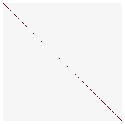
(a) GCA

(c) Ours

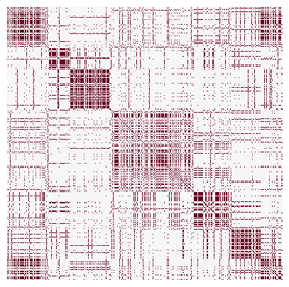
(b) SCAGC

(d) Ground truth

Figure 1: Visualization of the positive sample pairs selected by (a) GCA (Zhu et al. 2021), (b) SCAGC, (Xia et al. 2022d) and (c) the proposed method. The red dots denote the generated sample pairs. Specifically, if a point $(i,j)$ is selected as positive, the $i$-th sample from the first view and the $j$-th sample from the second view are integrated as a positive sample pair. (d) is the ground-truth cluster indicator. The sample order is rearranged to make samples from the same cluster beside each other. From the figures, we can find that our proposed positive sample extraction mechanism is more discriminative than the existing algorithms. As a consequence, the learned network is also more informative.

Introduction

Thanks to the strong representation learning capacity of the graph data, Graph Neural Networks (GNNs) have been successfully applied to various applications, such as node classification (Kipf and Welling 2017; Veličković et al. 2017; Duan et al. 2022b; Wang et al. 2020, 2021d; Liu et al. 2022e; Yang et al. 2022b), graph classification (Wang et al. 2018b; Liu et al. 2021), time series analysis(Liu and Liu 2021; Liu, Wu, and Liu 2022; Xie et al. 2022), knowledge graph(Liang et al. 2022a, b), and so on. Among all the directions in graph learning, deep graph clustering is a fundamental yet challenging unsupervised task, which has become a hot research spot recently (Wang et al. 2019; Tu et al. 2020; Liu et al. 2022b, c).

Contrastive learning, which could capture the supervision information implicitly without human annotations, has become a prominent technique in deep graph clustering. Although promising performance has been achieved, we observe two issues in the contrastive sample-pair construction process. 1) The quality of positive samples heavily depends on the carefully selected graph data augmentations. However, inappropriate graph data augmentations, like random attribute permutation and random edge drop-out, would easily lead to semantic drift (Lee, Lee, and Park 2021), and indiscriminative positive samples. 2) The constructed negative samples are not reliable enough since the existing algorithms neglect to exploit the important clustering information. Concretely, the existing methods randomly select negative samples, which loosely assign negative labels to samples from the same category. To improve the quality of negative samples, GDCL (Zhao et al. 2021) and SCAGC (Xia et al. 2022d) randomly select samples from the different clusters. Although verified to be effective, the current clustering-result-based methods heavily rely on the carefully designed graph data augmentation and the well pre-trained model, thus limiting the clustering performance.

To solve these issues, we propose a novel Cluster-guided Contrastive deep Graph Clustering method, i.e., CCGC. Concretely, to construct two node views with different semantics, we take advantage of the Siamese encoders and make the parameters un-shared between two sub-networks. In this way, complex structure- and attribute-level data augmentations are avoided while the semantic drift problem has also been solved.

After that, we carefully select and construct the positive samples from the same cluster in two views according to high-confidence clustering pseudo labels. In this manner, we improve the discriminative capacity of the positive samples. As shown in Fig. 1, we visualize the positive sample pairs constructed by (a) GCA (Zhu et al. 2021), (b) SCAGC (Xia et al. 2022d), (c) our methods. It is clearly observed that our constructed positive samples could better reveal the ground truth compared to other methods. Meanwhile, we regard the centers of different high-confidence clusters as the negative sample pairs, which are more reliable and semantic meaningful. Moreover, we design an objective function to pull close the samples from the same cluster and push away those from different clusters by maximizing and minimizing the cross-view cosine similarity between positive and negative samples. The key contributions of this paper are listed as follows:

• We propose a cluster-guided contrastive deep graph clustering network termed CCGC to improve the quality of positive and negative samples by mining the high-confidence clustering information.

• Instead of using carefully designed complex graph data augmentation, we conduct two views by designing special un-shared parameters Siamese encoders, thus avoiding semantic drift caused by inappropriate graph data augmentations.

• Extensive experimental results on six benchmark datasets demonstrate the effectiveness of the proposed method against the existing state-of-the-art deep graph clustering competitors.

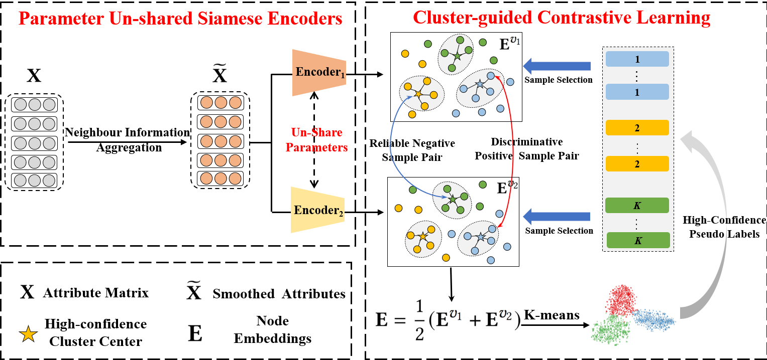
Figure 2: Illustration of the Cluster-guided Contrastive Graph Clustering (CCGC) algorithm. In our proposed algorithm, we firstly encode the two-view node embeddings with the proposed parameter un-shared Siamese encoders. Then, we perform K-means on the fused node embeddings and obtain the clustering results. Subsequently, based on the high-confidence clustering results, we improve the quality of positive and negative samples by the discriminative positive sample construction strategy and reliable negative sample construction strategy in section Cluster-guided Contrastive Learning. Lastly, we design an objective function to pull close the samples from the same cluster while pushing away different high-confidence cluster centers, thus enhancing the discriminative capability of the network.

Related Work

Deep Graph Clustering

Clustering is a fundamental yet challenging task, which aims to learn node semantic representations and divide nodes into different clusters (Liu et al. 2022a; Zhang et al. 2020; Sun et al. 2021b; Wan et al. 2022; Xia et al. 2022c, e). Deep learning methods also attract attention (Zhou et al. 2020). Among those methods, deep graph clustering has been a hot research spot in recent years. According to the learning mechanism, the existing methods can be roughly grouped into three classes including generative methods, adversarial methods, and contrastive methods. Our survey paper (Liu et al. 2022c) summarizes the detailed information about the fast-growing deep graph clustering. CCGC is categorized into the last one, i.e., contrastive methods. This section reviews the generative methods and adversarial methods, and the contrastive methods will be detailed in the next section.

Inspired by the success of graph-auto-encoder (GAE) (Kipf and Welling 2016), the pioneer MGAE (Wang et al. 2017) first encodes the nodes with the graph-encoder (Kipf and Welling 2016) and then performs clustering on the latent features. After that, DAEGC (Wang et al. 2019) adopts the attention mechanisms (Vaswani et al. 2017; Veličković et al. 2017) in early works to improve the clustering performance. Furthermore, ARGA (Pan et al. 2019) and AGAE (Tao et al. 2019) improve the discriminative capability of samples by adversarial mechanisms (Wang et al. 2018a). In addition, SDCN (Bo et al. 2020) alleviates the over-smoothing problem by integrating GAE and auto-encoder into the unified framework. More recently, R-GAE (Liu et al. 2022d) enhances the existing GAE-based methods by alleviating the feature randomness and feature drift issues.

Although verified to be effective, since most of these methods adopt a distribution alignment loss function (Xie, Girshick, and Farhadi 2016) to force the learned node embeddings to have the minimum distortion against the pre-learned cluster centers, their clustering performance is highly dependent on good initial cluster centers, thus leading to manual trial-and-error pre-training (Wang et al. 2019; Pan et al. 2019; Bo et al. 2020; Tu et al. 2020). As a consequence, the performance consistency, as well as the implementing convenience, is largely decreased. Different from them, several contrastive methods (Hassani and Khasahmadi 2020; Cui et al. 2020; Pan and Kang 2021) replace the clustering guided loss function by the contrastive loss, thus getting rid of trial-and-error pre-training.

Contrastive Deep Graph Clustering

Contrastive learning has achieved great success in the fields of computer vision (Yang et al. 2022a) and graph learning (Xia et al. 2022a; Wang et al. 2021c; Yu et al. 2022; Duan et al. 2022a) in recent years. Inspired by their success, contrastive deep graph clustering methods (Liu et al. 2022b, f; Zhao et al. 2021) are increasingly proposed.

The fashions of the data augmentations and the positive-negative sample pair construction are two crucial factors to determine the performance of the contrastive deep graph clustering methods. In this section, we review the existing contrastive methods from these two perspectives.

Data augmentation. The technique of data augmentation plays an important role in contrastive deep graph clustering. Specifically, the existing methods construct different views of the graph by applying distinct augmentations to the graph. For example, the graph diffusion matrix would be regarded as one of the augmented graphs in MVGRL (Hassani and Khasahmadi 2020), GDCL (Zhao et al. 2021), and DCRN (Liu et al. 2022b). Differently, SCAGC (Xia et al. 2022d) randomly adds or drops edges to perturb the structure of graphs. From the feature perspective, DCRN and SCAGC conduct augmentations on node attributes by attribute corruption. Although verified to be effective, the promising performance of these methods highly depends on the carefully selected data augmentations. Some works (Lee, Lee, and Park 2021; Sun et al. 2021a) point out that the inappropriate data augmentations would easily lead to semantic drift and the similar conclusion could be found in section Effectiveness of Parameter Un-shared Encoders. To overcome the issue, we propose a novel augmentation fashion to construct different graph views by setting the parameters of Siamese encoders to be un-shared, thus avoiding the semantic drift caused by inappropriate augmentations.

Positive and negative sample pair construction. Another crucial component in contrastive methods is the fashion of the positive and negative sample pair construction. Specifically, contrastive methods pull together positive samples while pushing away negative ones, thus the quality of positive and negative samples determines the performance of contrastive methods. Concretely, MVGRL (Hassani and Khasahmadi 2020) regards different augmented views of the same node and generates the negative samples by randomly shuffling the feature. Besides, DCRN (Liu et al. 2022b) pulls together the same node in different views while pushing away different nodes under the feature decorrelation constrain. Moreover, SCAGC (Xia et al. 2022d) and GDCL (Zhao et al. 2021) improve the quality of negative samples by randomly selecting samples from the different clusters. Although verified to be effective, they still rely on a well pre-trained model to select high-quality positive and negative samples. To solve this problem, we propose a high-confidence clustering information guided fashion of positive and negative sample construction, thus enhancing the discriminative capability and reliability of the sample pairs.

Method

In this section, we propose a novel Cluster-guided Contrastive deep Graph Clustering algorithm (CCGC). The overall framework of CCGC is shown in Fig. 2. In the following sections, we will introduce the proposed CCGC in specific.

Notations and Problem Definition

In an undirected graph $\mathcal{G}=\left\{\textbf{X},\textbf{A}\right\}$, let $\mathcal{V}=\{v_{1},v_{2},\dots,v_{N}\}$ be a set of $N$ nodes with $K$ classes and $\mathcal{E}$ be a set of edges. $\textbf{X}\in\mathds{R}^{N\times D}$ and $\textbf{A}\in\mathds{R}^{N\times N}$ denote the attribute matrix and the original adjacency matrix, respectively. The degree matrix is formulated as $\textbf{D}=diag(d_{1},d_{2},\dots,d_{N})\in\mathds{R}^{N\times N}$ and $d_{i}=\sum_{(v_{i},v_{j})\in\mathcal{E}}a_{ij}$. The graph Laplacian matrix is defined as $\textbf{L}=\textbf{D}-\textbf{A}$. With the renormalization trick $\widehat{\textbf{A}}=\textbf{A}+\textbf{I}$, the symmetric normalized graph Laplacian matrix is denoted as $\widetilde{\textbf{L}}=\textbf{I}-\widehat{\textbf{D}}^{-\frac{1}{2}}\widehat{\textbf{A}}\widehat{\textbf{D}}^{-\frac{1}{2}}$.

Parameter Un-shared Siamese Encoders

In this section, following SCGC (Liu et al. 2022d), we embed the nodes into the latent space and construct two different sample views by designing a parameter un-shared Siamese encoders.

Before encoding, we adopt a widely-used Laplacian filter (Cui et al. 2020) to conduct neighbour information aggregation as follows:

$$\widetilde{\textbf{X}}=(\textbf{I}-\widetilde{\textbf{L}})^{t}\textbf{X},$$ (1)

where $\widetilde{\textbf{L}}$ is the symmetric normalized graph Laplacian matrix. $t$ denotes the layer number of the Laplacian filter. $\widetilde{\textbf{X}}$ is the smoothed attribute matrix. Then we encode $\widetilde{\textbf{X}}$ with MLP encoders as follows:

$$\textbf{E}^{v_{1}}=\text{Encoder}_{1}(\widetilde{\textbf{X}}),\ \textbf{E}^{v_{2}}=\text{Encoder}_{2}(\widetilde{\textbf{X}}),$$ (2)

where $\textbf{E}^{v_{1}}$ and $\textbf{E}^{v_{2}}$ denotes the first and second view of the node embeddings, respectively. For the encoders, we design them to have the same architecture but un-shared learnable parameters. Subsequently, we normalize $\textbf{E}^{v_{1}}$ and $\textbf{E}^{v_{2}}$ with ${\ell^{2}}$-norm:

$$\textbf{E}^{v_{1}}=\frac{\textbf{E}^{v_{1}}}{||\textbf{E}^{v_{1}}||_{2}},\ \textbf{E}^{v_{2}}=\frac{\textbf{E}^{v_{2}}}{||\textbf{E}^{v_{2}}||_{2}}.$$ (3)

By this setting, we construct two node views with different semantic, thus avoiding semantic drift caused by inappropriate data augmentations on the graphs. Experimental evidence could be found in section Effectiveness of Parameter Un-shared Encoders.

Cluster-guided Contrastive Learning

In this section, we propose the Cluster-guided Contrastive Learning (CCL) to improve the discriminative capability and reliability of samples by mining the high-confidence clustering information.

To be specific, we firstly fuse the two views of the node embeddings as follows:

$$\textbf{E}=\frac{1}{2}(\textbf{E}^{v_{1}}+\textbf{E}^{v_{2}}).$$ (4)

Then we perform K-means on E and obtain the clustering results. In order to generate more reliable clustering information (Liu et al. 2022f), we define the confidence score $\textbf{CONF}_{i}$ of $i$-th sample as formulated:

$$\textbf{CONF}_{i}=e^{-||\textbf{E}_{i}-\textbf{C}_{p}||^{2}},$$ (5)

where $\textbf{E}_{i}$ denotes the $i$-th node embedding. Besides, $\textbf{C}_{p}(p=1,2,...,K)$ denotes the center of the cluster, which contains the $i$-th sample. Subsequently, based on CONF, we denote the high-confidence sample indexes $h$ as follows:

$$h=\{h_{1},h_{2},...,h_{i},...\},$$ (6)

where the element $h_{i}$ indicates that $h_{i}$-th sample belongs to top $\tau$ high-confidence sample set.

Based on these high-confidence samples and their clustering pseudo labels, we propose two sample construction strategies including Discriminative Positive sample construction Strategy (DPS) and Reliable Negative sample construction Strategy (RNS).

Discriminative Positive Sample Construction Strategy. In this part, we design DPS to enhance the discriminative capability of positive samples. The proposed DPS contains three steps. Firstly, we select the high-confidence samples of two views with high-confidence indexes $h$ as follows:

$$\textbf{H}^{v_{1}}=\textbf{E}^{v_{1}}_{[h,:]},\ \textbf{H}^{v_{2}}=\textbf{E}^{v_{2}}_{[h,:]}.$$ (7)

Then, according to the corresponding pseudo labels, we group $\textbf{H}^{v_{1}}$ and $\textbf{H}^{v_{2}}$ into $K$ disjoint clusters, i.e., $\textbf{B}^{v_{1}}_{p}(p=1,2,...,K)$, and $\textbf{B}^{v_{2}}_{q}(q=1,2,...,K)$. Subsequently, the positive samples will be selected and constructed from the same high-confidence clusters in Eq. (9). In this setting, the high-confidence clustering pseudo labels could be utilized as the supervisory information to improve the discriminative capability of the positive samples.

Reliable Negative Sample Construction Strategy. For the negative sample construction, the existing works (Zhu et al. 2021; Liu et al. 2022b) directly regard all other non-positive samples as negative samples, easily bringing false-negative samples. To alleviate this issue, we propose RNS, which contains two steps. Concretely, we first calculate the centers of high-confidence samples in two views:

$$\textbf{CEN}^{v_{1}}_{p} =avg(\textbf{B}^{v_{1}}_{p}),p=1,2,...,K,$$ (8)

$$\textbf{CEN}^{v_{2}}_{q} =avg(\textbf{B}^{v_{2}}_{q}),q=1,2,...,K,$$

where $avg$ is the average function. Then we regard the different high-confidence centers as the negative samples in Eq. (10). In this manner, RNS would enhance the reliability of negative samples, thus reducing the possibility of false-negative samples.

In summary, the proposed CCL would guide our network to mine the supervisory information in the high-confidence clustering pseudo labels, thus improving the discriminative capability and reliability of samples.

MGAE

DAEGC

ARGA

SDCN

DFCN

AGE

MVGRL

AutoSSL

AGC-DRR

AFGRL

GDCL

ProGCL

CCGC

Dataset

Metrix

CIKM 17

IJCAI 19

IJCAI 19

WWW 20

AAAI 21

SIGKDD 20

ICML 20

ICLR 22

IJCAI 22

AAAI 22

IJCAI 21

ICML 22

Ours

ACC

43.38±2.11

70.43±0.36

71.04±0.25

35.60±2.83

36.33±0.49

73.50±1.83

70.47±3.70

63.81±0.57

40.62±0.55

26.25±1.24

70.83±0.47

57.13+1.23

73.88±1.20

NMI

28.78±2.97

52.89±0.69

51.06±0.52

14.28±1.91

19.36±0.87

57.58±1.42

55.57±1.54

47.62±0.45

18.74±0.73

12.36±1.54

56.30±0.36

41.02+1.34

56.45±1.04

ARI

16.43±1.65

49.63±0.43

47.71±0.33

07.78±3.24

04.67±2.10

50.10±2.14

48.70±3.94

38.92±0.77

14.80±1.64

14.32±1.87

48.05±0.72

30.71+2.70

52.51±1.89

CORA

F1

33.48±3.05

68.27±0.57

69.27±0.39

24.37±1.04

26.16±0.50

69.28±1.59

67.15±1.86

56.42±0.21

31.23±0.57

30.20±1.15

52.88±0.97

45.68+1.29

70.98±2.79

ACC

61.35±0.80

64.54±1.39

61.07±0.49

65.96±0.31

69.50±0.20

69.73±0.24

62.83±1.59

66.76±0.67

68.32±1.83

31.45±0.54

66.39±0.65

65.92+0.80

69.84±0.94

NMI

34.63±0.65

36.41±0.86

34.40±0.71

38.71±0.32

43.90±0.20

44.93±0.53

40.69±0.93

40.67±0.84

43.28±1.41

15.17±0.47

39.52±0.38

39.59+0.39

44.33±0.79

ARI

33.55±1.18

37.78±1.24

34.32±0.70

40.17±0.43

45.50±0.30

45.31±0.41

34.18±1.73

38.73±0.55

45.34±2.33

14.32±0.78

41.07±0.96

36.16+1.11

45.68±1.80

CITESEER

F1

57.36±0.82

62.20±1.32

58.23±0.31

63.62±0.24

64.30±0.20

64.45±0.27

59.54±2.17

58.22±0.68

64.82±1.60

30.20±0.71

61.12±0.70

57.89+1.98

62.71±2.06

ACC

71.57±2.48

75.96±0.23

69.28±2.30

53.44±0.81

76.82±0.23

75.98±0.68

41.07±3.12

54.55±0.97

76.81±1.45

75.51±0.77

43.75±0.78

51.53+0.38

77.25±0.41

NMI

62.13±2.79

65.25±0.45

58.36±2.76

44.85±0.83

66.23±1.21

65.38±0.61

30.28±3.94

48.56±0.71

66.54±1.24

64.05±0.15

37.32±0.28

39.56+0.39

67.44±0.48

ARI

48.82±4.57

58.12±0.24

44.18±4.41

31.21±1.23

58.28±0.74

55.89±1.34

18.77±2.34

26.87±0.34

60.15±1.56

54.45±0.48

21.57±0.51

34.18+0.89

57.99±0.66

AMAP

F1

68.08±1.76

69.87±0.54

64.30±1.95

50.66±1.49

71.25±0.31

71.74±0.93

32.88±5.50

54.47±0.83

71.03±0.64

69.99±0.34

38.37±0.29

31.97+0.44

72.18±0.57

ACC

53.59±2.04

52.67±0.00

67.86±0.80

53.05±4.63

55.73±0.06

56.68±0.76

37.56±0.32

42.43±0.47

47.79±0.02

50.92±0.44

45.42±0.54

55.73+0.79

75.04±1.78

NMI

30.59±2.06

21.43±0.35

49.09±0.54

25.74±5.71

48.77±0.51

36.04±1.54

29.33±0.70

17.84±0.98

19.91±0.24

27.55±0.62

31.70±0.42

28.69+0.92

50.23±2.43

ARI

24.15±1.70

18.18±0.29

42.02±1.21

21.04±4.97

37.76±0.23

26.59±1.83

13.45±0.03

13.11±0.81

14.59±0.13

21.89±0.74

19.33±0.57

21.84+1.34

46.95±3.09

BAT

F1

50.83±3.23

52.23±0.03

67.02±1.15

46.45±5.90

50.90±0.12

55.07±0.80

29.64±0.49

34.84±0.15

42.33±0.51

46.53±0.57

39.94±0.57

56.08+0.89

74.90±1.80

ACC

44.61±2.10

36.89±0.15

52.13±0.00

39.07±1.51

49.37±0.19

47.26±0.32

32.88±0.71

31.33±0.52

37.37±0.11

37.42±1.24

33.46±0.18

43.36+0.87

57.19±0.66

NMI

15.60±2.30

05.57±0.06

22.48±1.21

08.83±2.54

32.90±0.41

23.74±0.90

11.72±1.08

07.63±0.85

07.00±0.85

11.44±1.41

13.22±0.33

23.93+0.45

33.85±0.87

ARI

13.40±1.26

05.03±0.08

17.29±0.50

06.31±1.95

23.25±0.18

16.57±0.46

04.68±1.30

02.13±0.67

04.88±0.91

06.57±1.73

04.31±0.29

15.03+0.98

27.71±0.41

EAT

F1

43.08±3.26

34.72±0.16

52.75±0.07

33.42±3.10

42.95±0.04

45.54±0.40

25.35±0.75

21.82±0.98

35.20±0.17

30.53±1.47

25.02±0.21

42.54+0.45

57.09±0.94

ACC

48.97±1.52

52.29±0.49

49.31±0.15

52.25±1.91

33.61±0.09

52.37±0.42

44.16±1.38

42.52±0.64

42.64±0.31

41.50±0..25

48.70±0.06

45.38+0.58

56.34±1.11

NMI

20.69±0.98

21.33±0.44

25.44±0.31

21.61±1.26

26.49±0.41

23.64±0.66

21.53±0.94

17.86±0.22

11.15±0.24

17.33±0.54

25.10±0.01

22.04+2.23

28.15±1.92

ARI

18.33±1.79

20.50±0.51

16.57±0.31

21.63±1.49

11.87±0.23

20.39±0.70

17.12±1.46

13.13±0.71

09.50±0.25

13.62±0.57

21.76±0.01

14.74+1.99

25.52±2.09

UAT

F1

47.95±1.52

50.33±0.64

50.26±0.16

45.59±3.54

25.79±0.29

50.15±0.73

39.44±2.19

34.94±0.87

35.18±0.32

36.52±0.89

45.69±0.08

39.30+1.82

55.24±1.69

Table 1: The average clustering performance of ten runs on six benchmark datasets. The performance is evaluated by four metrics with mean value and standard deviation. The red and blue values indicate the best and the runner-up results, respectively.

Objective Function

The proposed method jointly optimizes two objectives including the positive sample loss $\mathcal{L}_{pos}$ and the negative sample loss $\mathcal{L}_{neg}$.

In detail, $\mathcal{L}_{pos}$ is the Mean Squared Error (MSE) loss between the normalized cross-view positive sample embeddings, as formulated:

$$\mathcal{L}_{pos} =\frac{1}{K}\sum_{p=1}^{K}\sum_{i=1}^{n_{p}}\left\|\textbf{B}^{v_{1}}_{p[i,:]}-\textbf{B}^{v_{2}}_{p[i,:]}\right\|^{2}_{2}$$ (9)

$$=\frac{1}{K}\sum_{p=1}^{K}\sum_{i=1}^{n_{p}}\left(2-2\left\langle\textbf{B}^{v_{1}}_{p[i,:]},\textbf{B}^{v_{2}}_{p[i,:]}\right\rangle\right),$$

where $\textbf{B}^{v_{1}}_{p[i,:]}$ and $\textbf{B}^{v_{2}}_{p[i,:]}$ denotes the $i$-th normalized node embedding in the $p$-th cluster of the first and second view, respectively. Besides, $n_{p}$ is the number of high-confidence samples in the $p$-th cluster. In this manner, the positive samples are pulled together. Besides, we define $\mathcal{L}_{neg}$ as the cosine similarity between different centers of the high-confidence embeddings:

$$\mathcal{L}_{neg} =\frac{1}{K^{2}-K}\sum_{p=1}^{K}\sum_{q=1}^{K}\frac{\left\langle\textbf{CEN}_{p}^{v_{1}},\textbf{CEN}_{q}^{v_{2}}\right\rangle}{\|\textbf{CEN}_{p}^{v_{1}}\|_{2}\cdot\|\textbf{CEN}_{q}^{v_{2}}\|_{2}},p\neq q,$$ (10)

where $\textbf{CEN}_{p}^{v_{1}}$ is the $p$-th high-confidence center in the first view and $\textbf{CEN}_{q}^{v_{2}}$ is the $q$-th high-confidence center in the second view. By setting this, we push the negative samples away.

In summary, the total loss of the proposed CCGC is calculated as:

$$\mathcal{L}=\mathcal{L}_{pos}+\alpha\mathcal{L}_{neg},$$ (11)

where $\alpha$ is a trade-off between $\mathcal{L}_{pos}$ and $\mathcal{L}_{neg}$. The detailed learning process of CCGC is shown in Algorithm 1.

Experiments

Benchmark Datasets

The experiments are conducted on six widely-used benchmark datasets, including CORA (Cui et al. 2020), CITESEER (Cui et al. 2020), BAT (Liu et al. 2022d; Mrabah et al. 2021), EAT (Liu et al. 2022d), UAT (Liu et al. 2022d), AMAP (Liu et al. 2022b). The summarized information is shown in Table 2.

Dataset	Type	Sample	Dimension	Edge	Class
CORA	Graph	2708	1433	5429	7
CITESEER	Graph	3327	3703	4732	6
AMAP	Graph	7650	745	119081	8
BAT	Graph	131	81	1038	4
EAT	Graph	399	203	5994	4
UAT	Graph	1190	239	13599	4

Table 2: Statistics summary of six datasets.

Experiment Setup

The experimental environment contains one desktop computer with the Intel Core i7-7820x CPU, one NVIDIA GeForce RTX 2080Ti GPU, 64GB RAM, and the PyTorch deep learning platform. The max training epoch number is set to 400. We minimize the total loss in Eq. (11) with widely-used Adam optimizer (Kingma and Ba 2014) and then perform K-means over the learned embeddings. To obtain reliable clustering, we adopt a two-stage training strategy. The discriminative capacity of the model can be improved in the first stage. In the second stage, the contrastive learning mechanism can be enhanced by the high-confidence clustering pseudo labels. Ten runs are conducted for all methods. For the baselines, we adopt their source with original settings and reproduce the results. The hyper-parameter settings are summarized in Table 1 of the Appendix. The clustering performance is evaluated by four metrics including ACC, NMI, ARI, and F1 (Zhou et al. 2019; Wang et al. 2021b, a; Li et al. 2022).

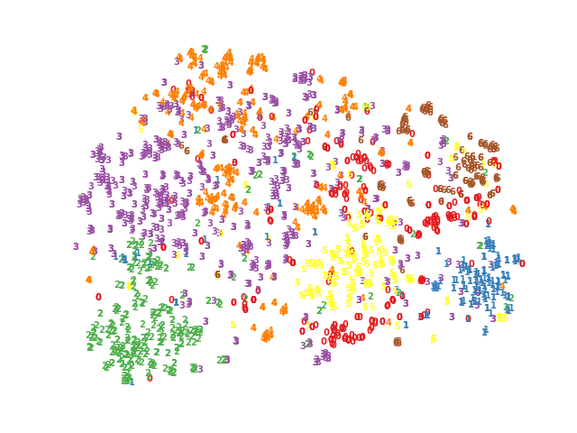
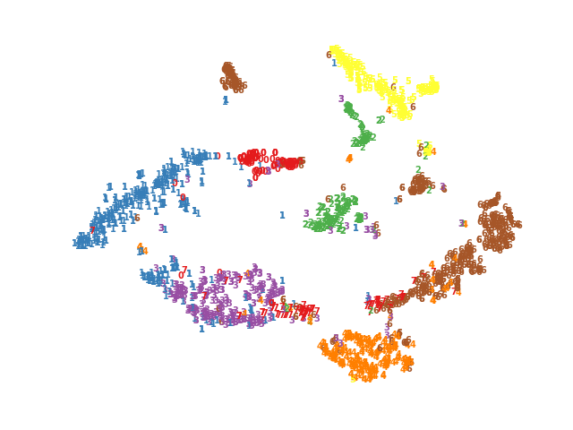
DAEGC

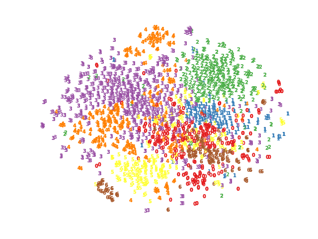
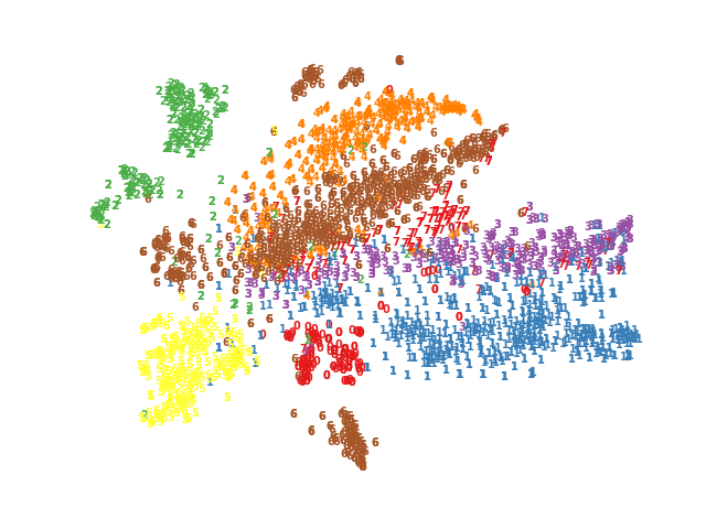
MVGRL

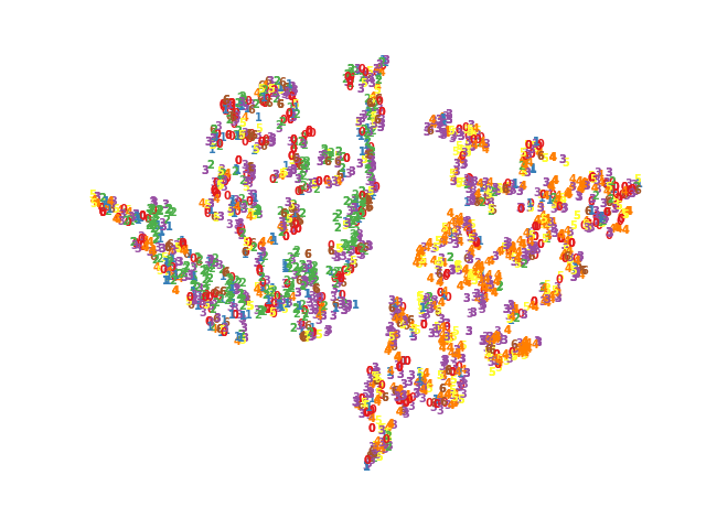
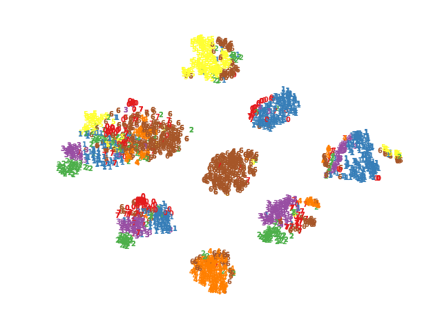
SDCN

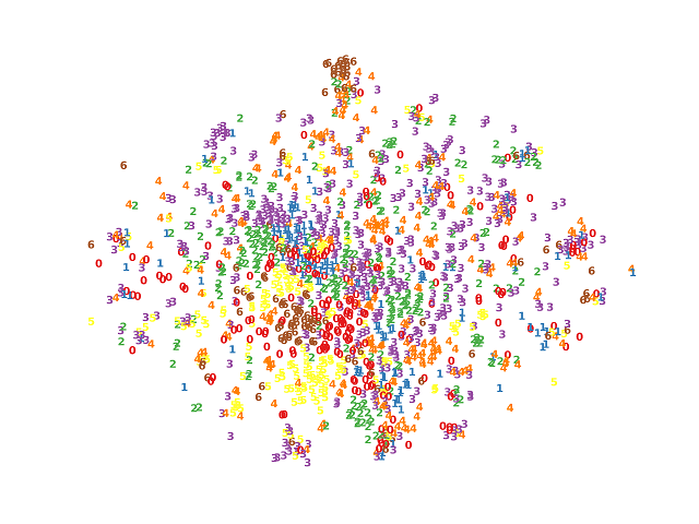
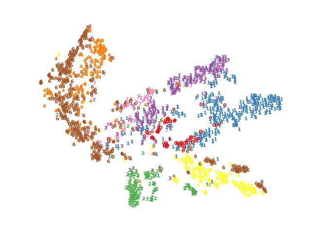
AutoSSL

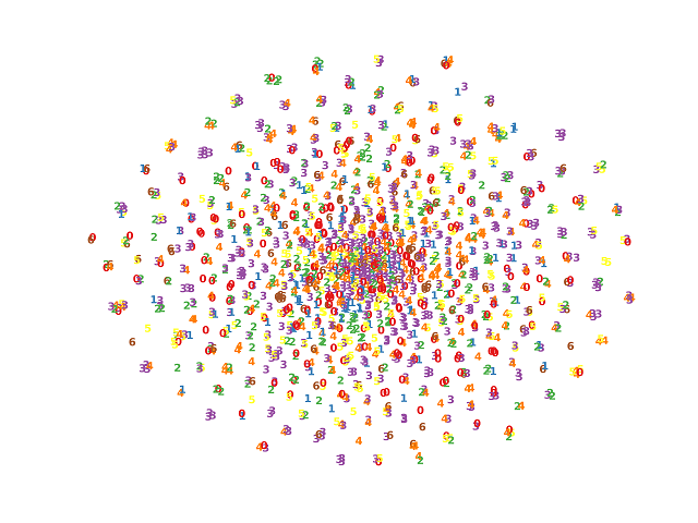
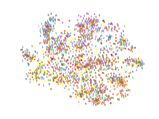
AFGRL

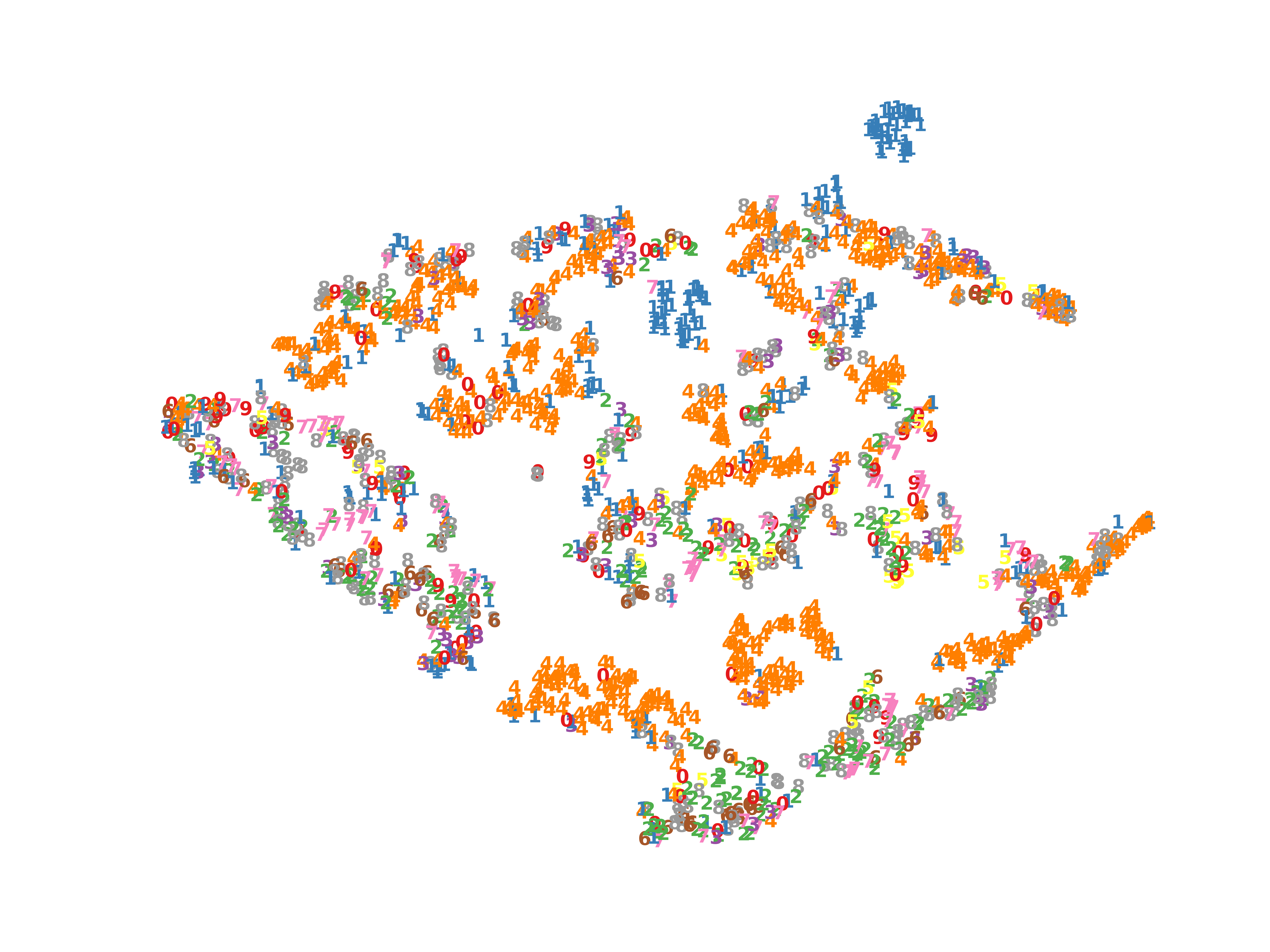
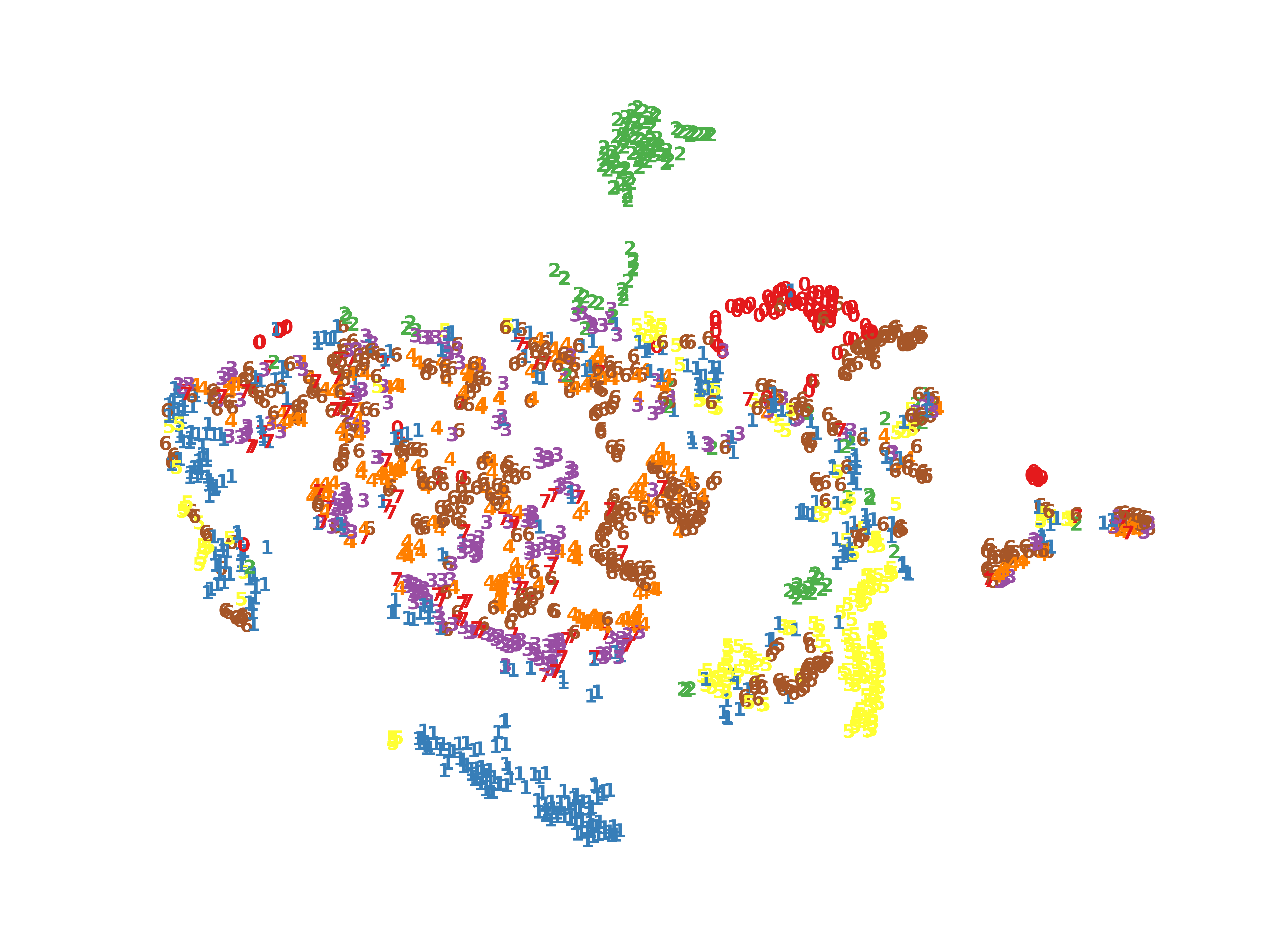
GDCL

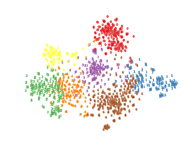
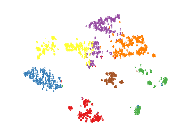
Ours

Figure 3: 2D visualization on two datasets. The first row and second row correspond to CORA and AMAP, respectively.

Algorithm 1 CCGC

Performance Comparison

In this subsection, we compare the clustering performance of our proposed algorithm with baselines on six datasets with four metrics. Among these methods, five classical deep graph clustering methods (Wang et al. 2017, 2019; Pan et al. 2019; Bo et al. 2020; Tu et al. 2020) utilize the graph auto-encoder to learn the node representation for clustering. Besides, seven contrastive deep graph clustering methods (Cui et al. 2020; Hassani and Khasahmadi 2020; Jin et al. 2021; Gong et al. 2022; Lee, Lee, and Park 2021; Zhao et al. 2021; Xia et al. 2022b) improve the discriminative capability of samples by the contrastive strategies.

From the results in Table.1, we find that CCGC obtains better performance compared with the classical deep graph clustering methods. The reason is that contrastive learning could assist the model capture the supervision information implicitly. Besides, the contrastive methods achieve sub-optimal performance compared to ours. This is because we improve the discriminative capability and reliability of samples with the important clustering information. In summary, our method outperforms most of them on six datasets with four metrics. Taking the results on EAT dataset for example, CCGC exceeds the runner-up by 5.06%, 9.92%, 4.46%, 4.34% with respect to ACC, NMI, ARI, and F1. Besides, due to the limitation of the space, we conduct additional comparison experiments with nine baselines. Those results are shown in Table 2 of the Appendix. The results could also demonstrate the superiority of CCGC.

Ablation Studies

In this section, we first verify the effectiveness of two proposed sample construction strategies with experiments. Besides, we demonstrate the effect of parameter un-shared encoders and analyze the sensitivity of hyper-parameters in CCGC.

Dataset	Metric	(w/o) Positive	(w/o) Negitive	Drop Edges	Add Edges	Diffusion	Mask Feature	Ours
	ACC	60.03±6.28	70.29±0.86	57.95±4.32	57.89±3.16	59.57±2.95	67.40±1.76	73.88±1.20
	NMI	47.33±3.97	53.67±1.15	39.32±4.90	39.11±3.82	39.84±2.72	48.84±2.02	55.56±1.04
	ARI	37.66±5.86	47.09±1.29	29.10±4.52	29.74±2.84	30.73±2.95	41.32±2.33	52.51±1.89
CORA	F1	53.85±9.38	68.48±1.17	53.45±5.57	55.33± 6.39	55.01±7.22	63.16±3.54	70.98±2.79
	ACC	58.26±6.19	67.92±1.32	66.55±1.27	66.31±1.40	68.32±0.62	69.14±0.66	69.84±0.94
	NMI	38.62±3.34	42.05±1.34	38.91±2.04	39.43±1.72	41.83±0.94	42.49±0.89	44.33±0.79
	ARI	35.78±4.28	42.66±1.65	38.85±1.63	39.00±1.32	41.23±0.99	43.12±1.16	44.68±1.80
CITESEER	F1	45.90±7.76	62.82±0.92	58.38±1.51	59.56±1.40	59.89±0.83	60.78±1.43	62.71±2.06
	ACC	29.81±1.71	73.74±0.82	75.84±1.12	75.75±1.77	70.89±3.28	76.48±1.88	77.25±0.41
	NMI	15.18±1.93	62.65±1.48	62.98±1.15	63.11±1.89	58.14±2.05	66.44±0.85	67.44±0.48
	ARI	05.85±0.95	52.74±1.51	55.81±1.63	55.79±2.85	49.68±3.16	56.81±2.09	57.99±0.66
AMAP	F1	26.61±3.49	68.45±1.08	69.82±3.24	69.83±3.13	60.43±6.16	71.13±1.40	72.18±0.57
	ACC	65.19±2.00	73.59±2.32	50.00±3.87	67.02±2.71	52.60±2.72	72.06±2.92	75.04±1.78
	NMI	44.08±1.35	47.07±2.38	24.59±2.01	45.13±4.73	29.78±5.06	48.67±2.47	50.23±2.43
	ARI	38.46±2.60	44.37±3.47	18.91±3.80	39.18±5.16	21.12±5.70	44.07±3.80	46.95±3.09
BAT	F1	62.24±2.57	73.36±2.35	48.44±4.90	65.54±2.66	48.72±2.54	71.57±3.46	74.90±1.80
	ACC	48.42±2.91	52.31±1.66	45.76±1.00	49.32±1.53	45.71±1.67	52.61±1.70	57.19±0.66
	NMI	25.88±2.73	26.12±2.07	14.57±3.14	23.45±2.00	19.98±1.84	27.18±1.55	33.85±0.87
	ARI	19.29±2.02	20.94±1.40	10.43±1.63	16.85±1.76	14.71±3.32	20.50±1.46	27.71±0.41
EAT	F1	46.39±4.98	52.63±1.90	43.78±1.36	48.99±2.18	40.46±3.81	52.51±2.02	57.09±0.94
	ACC	41.39±2.96	49.04±1.33	57.02±1.44	55.61±1.00	51.45±2.04	52.33±1.95	56.34±1.11
	NMI	12.08±1.86	22.89±1.71	26.07±1.43	29.06±1.49	24.18±2.19	24.12±1.99	28.15±1.92
	ARI	7.70±0.63	20.70±1.22	26.03±1.88	23.69±1.58	22.55±2.80	18.54±3.07	25.52±2.09
UAT	F1	36.14±3.32	44.22±2.24	54.67±1.67	54.74± 1.16	46.06±2.97	51.17±2.16	55.24±1.69

Table 3: Ablation studies of CCGC on six datasets.

Effectiveness of DPS and RNS

To verify the effect of the proposed Discriminative Positive sample construction Strategy (DPS) and Reliable Negative sample construction Strategy (RNS), we conduct extensive experiments as shown in Table 3. For simplicity, we denote “(w/o) DPS” and “(w/o) RNS” as replacing DPS and RNS in our model with the regular positive and negative sample construction fashion (Liu et al. 2022b), i.e., regarding the same samples in two view as positive samples while considering other samples as negative ones. From the observations, we conclude that the performance will decrease without any one of DPS and RNS, revealing that both strategies make essential contributions to boosting the performance. In addition, the quality of positive and negative sample pairs is improved compared with the regular sample construction fashion. Overall, the experimental results have verified the effectiveness of DPS and RNS.

Effectiveness of Parameter Un-shared Encoders

To avoid the complex augmentations on graphs, we design the un-shared Simases encoders to conduct two-node views. In this part, we compare our view construction method with other classical graph data augmentations including edge dropping (Xia et al. 2022d), edge adding (Xia et al. 2022d), graph diffusion (Hassani and Khasahmadi 2020), and feature masking (Zhao et al. 2021). Concretely, in Table 3, we first make the encoders in CCGC to share parameter and then adopt the data augmentation as randomly dropping 20% edges (“Drop Edges”), or randomly adding 20% edges (“Add Edges”), or graph diffusion (“Diffusion”) with 0.20 teleportation rate, or randomly masking 20% features (“Mask Features”). From the results, we observe that the commonly used graph augmentations might lead to semantic drift (Lee, Lee, and Park 2021), thus undermining the performance. In summary, expensive experiments have demonstrated the effectiveness of the proposed parameter un-shared encoders.

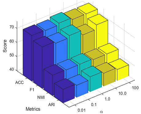
CORA

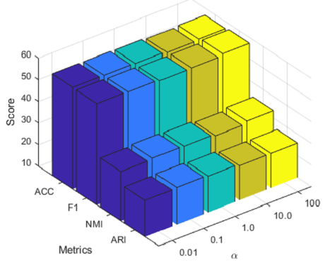
EAT

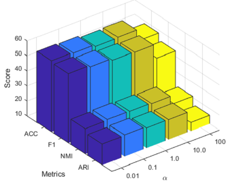
UAT

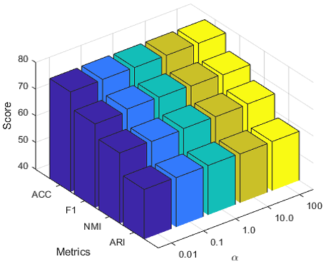
AMAP

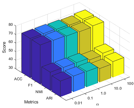
BAT

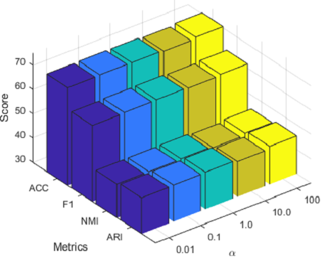
CITESEER

Figure 4: Sensitivity analysis of the hyper-parameter $\alpha$ on six datasets.

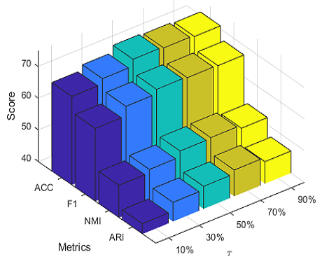
CORA

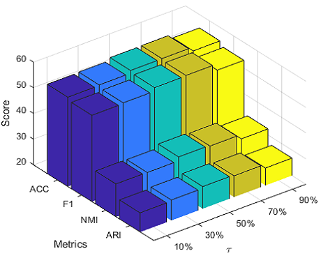
EAT

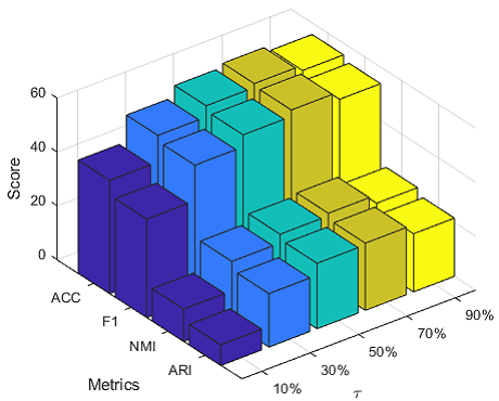
UAT

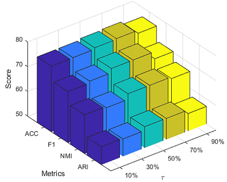
AMAP

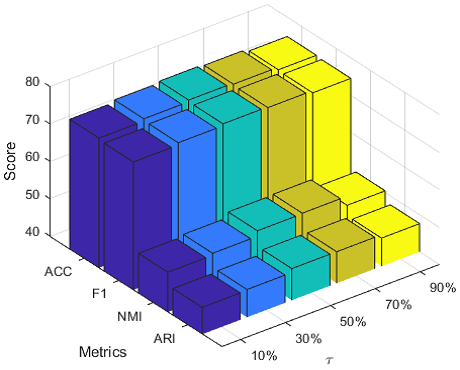
BAT

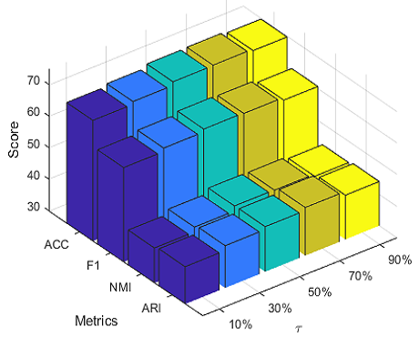
CITESEER

Figure 5: Sensitivity analysis of the hyper-parameter $\tau$ on six datasets.

Hyper-parameter Analysis

Sensitivity Analysis of hyper-parameter threshold $\tau$

We investigate the influence of the hyper-parameter threshold $\tau$ on six datasets as shown in Fig.5. From the results, we observe that the model obtains promising performance when $\tau\in[50\%,70\%]$. The reasons are as follows: 1) When $\tau<50\%$, the discriminative capacity of the network is limited due to few number of positive samples. 2) When $\tau>70\%$, the over-confidence pseudo labels would easily lead the network to confirmation bias (Arazo et al. 2020).

Sensitivity Analysis of hyper-parameter $\alpha$

Besides, to the trade-off hyper-parameter $\alpha$, the experimental results are shown in Fig.4. From these results, we observe that the performance will not fluctuate greatly when $\alpha$ is varying. This demonstrates that our CCGC is insensitive to $\alpha$. Moreover, CCGC is also insensitive to the layer number $t$ of Laplacian filters. Experimental evidences can be found in Fig. 1 in Appendix.

Visualization Analysis

In this part, we visualize the distribution of the learned embeddings of six baselines and CCGC to show the superiority of CCGC on CORA and AMAP datasets via $t$-SNE algorithm (Van der Maaten and Hinton 2008). As shown in Fig. 3, we can conclude that CCGC better reveals the intrinsic clustering structure compared with other baselines.

Conclusion

In this work, we propose a Cluster-guided Contrastive deep Graph Clustering network termed CCGC to improve the quality of positive and negative samples. To be specific, we firstly construct two views with the un-shared parameters Siamese encoders to avoid semantic drift caused by the inappropriate graph data augmentations. Besides, the proposed positive and negative samples construction strategies improve the discriminative capability and reliability of samples by mining the supervision information in the high-confidence clustering pseudo labels. Extensive experiments on six datasets demonstrate the effectiveness of our proposed method.

References

- Arazo et al. (2020) Arazo, E.; Ortego, D.; Albert, P.; O’Connor, N. E.; and McGuinness, K. 2020. Pseudo-labeling and confirmation bias in deep semi-supervised learning. In 2020 International Joint Conference on Neural Networks (IJCNN), 1–8. IEEE.
- Bo et al. (2020) Bo, D.; Wang, X.; Shi, C.; Zhu, M.; Lu, E.; and Cui, P. 2020. Structural deep clustering network. In Proceedings of The Web Conference 2020, 1400–1410.
- Cui et al. (2020) Cui, G.; Zhou, J.; Yang, C.; and Liu, Z. 2020. Adaptive graph encoder for attributed graph embedding. In Proceedings of the 26th ACM SIGKDD International Conference on Knowledge Discovery & Data Mining, 976–985.
- Duan et al. (2022a) Duan, J.; Wang, S.; Liu, X.; Zhou, H.; Hu, J.; and Jin, H. 2022a. GADMSL: Graph Anomaly Detection on Attributed Networks via Multi-scale Substructure Learning. arXiv preprint arXiv:2211.15255.
- Duan et al. (2022b) Duan, K.; Liu, Z.; Wang, P.; Zheng, W.; Zhou, K.; Chen, T.; Hu, X.; and Wang, Z. 2022b. A Comprehensive Study on Large-Scale Graph Training: Benchmarking and Rethinking. arXiv preprint arXiv:2210.07494.
- Gong et al. (2022) Gong, L.; Zhou, S.; Liu, X.; and Tu, W. 2022. Attributed Graph Clustering with Dual Redundancy Reduction. In IJCAI.
- Hassani and Khasahmadi (2020) Hassani, K.; and Khasahmadi, A. H. 2020. Contrastive multi-view representation learning on graphs. In International Conference on Machine Learning, 4116–4126. PMLR.
- Jin et al. (2021) Jin, W.; Liu, X.; Zhao, X.; Ma, Y.; Shah, N.; and Tang, J. 2021. Automated Self-Supervised Learning for Graphs. In International Conference on Learning Representations.
- Kingma and Ba (2014) Kingma, D. P.; and Ba, J. 2014. Adam: A method for stochastic optimization. arXiv preprint arXiv:1412.6980.
- Kipf and Welling (2016) Kipf, T. N.; and Welling, M. 2016. Variational graph auto-encoders. arXiv preprint arXiv:1611.07308.
- Kipf and Welling (2017) Kipf, T. N.; and Welling, M. 2017. Semi-supervised classification with graph convolutional networks. In International Conference on Learning Representations.
- Lee, Lee, and Park (2021) Lee, N.; Lee, J.; and Park, C. 2021. Augmentation-Free Self-Supervised Learning on Graphs. arXiv preprint arXiv:2112.02472.
- Li et al. (2022) Li, L.; Wang, S.; Liu, X.; Zhu, E.; Shen, L.; Li, K.; and Li, K. 2022. Local Sample-Weighted Multiple Kernel Clustering With Consensus Discriminative Graph. IEEE Transactions on Neural Networks and Learning Systems.
- Liang et al. (2022a) Liang, K.; Liu, Y.; Zhou, S.; Liu, X.; and Tu, W. 2022a. Relational Symmetry based Knowledge Graph Contrastive Learning.
- Liang et al. (2022b) Liang, K.; Meng, L.; Liu, M.; Liu, Y.; Tu, W.; Wang, S.; Zhou, S.; Liu, X.; and Sun, F. 2022b. Reasoning over Different Types of Knowledge Graphs: Static, Temporal and Multi-Modal. arXiv preprint arXiv:2212.05767.
- Liu and Liu (2021) Liu, M.; and Liu, Y. 2021. Inductive representation learning in temporal networks via mining neighborhood and community influences. In SIGIR.
- Liu, Wu, and Liu (2022) Liu, M.; Wu, J.-M.; and Liu, Y. 2022. Embedding Global and Local Influences for Dynamic Graphs. In CIKM.
- Liu et al. (2022a) Liu, S.; Wang, S.; Zhang, P.; Xu, K.; Liu, X.; Zhang, C.; and Gao, F. 2022a. Efficient one-pass multi-view subspace clustering with consensus anchors. In Proceedings of the AAAI Conference on Artificial Intelligence, volume 36, 7576–7584.
- Liu et al. (2021) Liu, X.; Jin, W.; Ma, Y.; Li, Y.; Liu, H.; Wang, Y.; Yan, M.; and Tang, J. 2021. Elastic graph neural networks. In International Conference on Machine Learning, 6837–6849. PMLR.
- Liu et al. (2022b) Liu, Y.; Tu, W.; Zhou, S.; Liu, X.; Song, L.; Yang, X.; and Zhu, E. 2022b. Deep Graph Clustering via Dual Correlation Reduction. In AAAI Conference on Artificial Intelligence.
- Liu et al. (2022c) Liu, Y.; Xia, J.; Zhou, S.; Wang, S.; Guo, X.; Yang, X.; Liang, K.; Tu, W.; Li, Z. S.; and Liu, X. 2022c. A Survey of Deep Graph Clustering: Taxonomy, Challenge, and Application. arXiv preprint arXiv:2211.12875.
- Liu et al. (2022d) Liu, Y.; Yang, X.; Zhou, S.; and Liu, X. 2022d. Simple Contrastive Graph Clustering. arXiv preprint arXiv:2205.0786.
- Liu et al. (2022e) Liu, Y.; Zheng, Y.; Zhang, D.; Chen, H.; Peng, H.; and Pan, S. 2022e. Towards unsupervised deep graph structure learning. In Proceedings of the ACM Web Conference 2022, 1392–1403.
- Liu et al. (2022f) Liu, Y.; Zhou, S.; Liu, X.; Tu, W.; and Yang, X. 2022f. Improved Dual Correlation Reduction Network. arXiv preprint arXiv:2202.12533.
- Mrabah et al. (2021) Mrabah, N.; Bouguessa, M.; Touati, M. F.; and Ksantini, R. 2021. Rethinking Graph Auto-Encoder Models for Attributed Graph Clustering. arXiv preprint arXiv:2107.08562.
- Pan and Kang (2021) Pan, E.; and Kang, Z. 2021. Multi-view contrastive graph clustering. Advances in neural information processing systems, 34: 2148–2159.
- Pan et al. (2019) Pan, S.; Hu, R.; Fung, S.-f.; Long, G.; Jiang, J.; and Zhang, C. 2019. Learning graph embedding with adversarial training methods. IEEE transactions on cybernetics, 50(6): 2475–2487.
- Sun et al. (2021a) Sun, M.; Xing, J.; Wang, H.; Chen, B.; and Zhou, J. 2021a. MoCL: Contrastive Learning on Molecular Graphs with Multi-level Domain Knowledge. arXiv preprint arXiv:2106.04509.
- Sun et al. (2021b) Sun, M.; Zhang, P.; Wang, S.; Zhou, S.; Tu, W.; Liu, X.; Zhu, E.; and Wang, C. 2021b. Scalable multi-view subspace clustering with unified anchors. In Proceedings of the 29th ACM International Conference on Multimedia, 3528–3536.
- Tao et al. (2019) Tao, Z.; Liu, H.; Li, J.; Wang, Z.; and Fu, Y. 2019. Adversarial graph embedding for ensemble clustering. In International Joint Conferences on Artificial Intelligence Organization.
- Tu et al. (2020) Tu, W.; Zhou, S.; Liu, X.; Guo, X.; Cai, Z.; Cheng, J.; et al. 2020. Deep Fusion Clustering Network. arXiv preprint arXiv:2012.09600.
- Van der Maaten and Hinton (2008) Van der Maaten, L.; and Hinton, G. 2008. Visualizing data using t-SNE. Journal of machine learning research, 9(11).
- Vaswani et al. (2017) Vaswani, A.; Shazeer, N.; Parmar, N.; Uszkoreit, J.; Jones, L.; Gomez, A. N.; Kaiser, Ł.; and Polosukhin, I. 2017. Attention is all you need. Advances in neural information processing systems, 30.
- Veličković et al. (2017) Veličković, P.; Cucurull, G.; Casanova, A.; Romero, A.; Lio, P.; and Bengio, Y. 2017. Graph attention networks. arXiv preprint arXiv:1710.10903.
- Wan et al. (2022) Wan, X.; Liu, J.; Liang, W.; Liu, X.; Wen, Y.; and Zhu, E. 2022. Continual Multi-View Clustering. In Proceedings of the 30th ACM International Conference on Multimedia, MM ’22, 3676–3684. New York, NY, USA: Association for Computing Machinery. ISBN 9781450392037.
- Wang et al. (2019) Wang, C.; Pan, S.; Hu, R.; Long, G.; Jiang, J.; and Zhang, C. 2019. Attributed graph clustering: A deep attentional embedding approach. arXiv preprint arXiv:1906.06532.
- Wang et al. (2017) Wang, C.; Pan, S.; Long, G.; Zhu, X.; and Jiang, J. 2017. Mgae: Marginalized graph autoencoder for graph clustering. In Proceedings of the 2017 ACM on Conference on Information and Knowledge Management, 889–898.
- Wang et al. (2018a) Wang, H.; Wang, J.; Wang, J.; Zhao, M.; Zhang, W.; Zhang, F.; Xie, X.; and Guo, M. 2018a. Graphgan: Graph representation learning with generative adversarial nets. In Proceedings of the AAAI conference on artificial intelligence, volume 32.
- Wang et al. (2021a) Wang, S.; Liu, X.; Liu, L.; Zhou, S.; and Zhu, E. 2021a. Late fusion multiple kernel clustering with proxy graph refinement. IEEE Transactions on Neural Networks and Learning Systems.
- Wang et al. (2021b) Wang, S.; Liu, X.; Zhu, X.; Zhang, P.; Zhang, Y.; Gao, F.; and Zhu, E. 2021b. Fast Parameter-Free Multi-View Subspace Clustering With Consensus Anchor Guidance. IEEE Transactions on Image Processing, 31: 556–568.
- Wang et al. (2021c) Wang, Y.; Cai, Y.; Liang, Y.; Ding, H.; Wang, C.; Bhatia, S.; and Hooi, B. 2021c. Adaptive data augmentation on temporal graphs. Advances in Neural Information Processing Systems, 34: 1440–1452.
- Wang et al. (2018b) Wang, Y.; Shi, Z.; Guo, X.; Liu, X.; Zhu, E.; and Yin, J. 2018b. Deep embedding for determining the number of clusters. In Proceedings of the AAAI Conference on Artificial Intelligence, volume 32.
- Wang et al. (2021d) Wang, Y.; Wang, W.; Liang, Y.; Cai, Y.; and Hooi, B. 2021d. Mixup for node and graph classification. In Proceedings of the Web Conference 2021, 3663–3674.
- Wang et al. (2020) Wang, Y.; Wang, W.; Liang, Y.; Cai, Y.; Liu, J.; and Hooi, B. 2020. Nodeaug: Semi-supervised node classification with data augmentation. In Proceedings of the 26th ACM SIGKDD International Conference on Knowledge Discovery & Data Mining, 207–217.
- Xia et al. (2022a) Xia, J.; Wu, L.; Chen, J.; Hu, B.; and Li, S. Z. 2022a. SimGRACE: A Simple Framework for Graph Contrastive Learning without Data Augmentation. arXiv preprint arXiv:2202.03104.
- Xia et al. (2022b) Xia, J.; Wu, L.; Wang, G.; Chen, J.; and Li, S. Z. 2022b. ProGCL: Rethinking Hard Negative Mining in Graph Contrastive Learning. In International Conference on Machine Learning, 24332–24346. PMLR.
- Xia et al. (2022c) Xia, W.; Gao, Q.; Wang, Q.; Gao, X.; Ding, C.; and Tao, D. 2022c. Tensorized Bipartite Graph Learning for Multi-View Clustering. IEEE Transactions on Pattern Analysis and Machine Intelligence.
- Xia et al. (2022d) Xia, W.; Wang, Q.; Gao, Q.; Yang, M.; and Gao, X. 2022d. Self-consistent Contrastive Attributed Graph Clustering with Pseudo-label Prompt. IEEE Transactions on Multimedia.
- Xia et al. (2022e) Xia, W.; Wang, Q.; Gao, Q.; Zhang, X.; and Gao, X. 2022e. Self-Supervised Graph Convolutional Network for Multi-View Clustering. IEEE Trans. Multim., 24: 3182–3192.
- Xie et al. (2022) Xie, F.; Zhang, Z.; Li, L.; Zhou, B.; and Tan, Y. 2022. EpiGNN: Exploring Spatial Transmission with Graph Neural Network for Regional Epidemic Forecasting. In Joint European Conference on Machine Learning and Knowledge Discovery in Databases. Springer.
- Xie, Girshick, and Farhadi (2016) Xie, J.; Girshick, R.; and Farhadi, A. 2016. Unsupervised deep embedding for clustering analysis. In International conference on machine learning, 478–487. PMLR.
- Yang et al. (2022a) Yang, X.; Hu, X.; Zhou, S.; Liu, X.; and Zhu, E. 2022a. Interpolation-Based Contrastive Learning for Few-Label Semi-Supervised Learning. IEEE Transactions on Neural Networks and Learning Systems, 1–12.
- Yang et al. (2022b) Yang, X.; Liu, Y.; Zhou, S.; Liu, X.; and Zhu, E. 2022b. Mixed Graph Contrastive Network for Semi-Supervised Node Classification. arXiv preprint arXiv:2206.02796.
- Yu et al. (2022) Yu, L.; Pei, S.; Ding, L.; Zhou, J.; Li, L.; Zhang, C.; and Zhang, X. 2022. SAIL: Self-Augmented Graph Contrastive Learning. In Proceedings of the AAAI Conference on Artificial Intelligence, volume 36, 8927–8935.
- Zhang et al. (2020) Zhang, P.; Liu, X.; Xiong, J.; Zhou, S.; Zhao, W.; Zhu, E.; and Cai, Z. 2020. Consensus one-step multi-view subspace clustering. IEEE Transactions on Knowledge and Data Engineering.
- Zhao et al. (2021) Zhao, H.; Yang, X.; Wang, Z.; Yang, E.; and Deng, C. 2021. Graph debiased contrastive learning with joint representation clustering. In Proc. IJCAI, 3434–3440.
- Zhou et al. (2019) Zhou, S.; Liu, X.; Li, M.; Zhu, E.; Liu, L.; Zhang, C.; and Yin, J. 2019. Multiple kernel clustering with neighbor-kernel subspace segmentation. IEEE transactions on neural networks and learning systems, 31(4): 1351–1362.
- Zhou et al. (2020) Zhou, S.; Nie, D.; Adeli, E.; Yin, J.; Lian, J.; and Shen, D. 2020. High-Resolution Encoder–Decoder Networks for Low-Contrast Medical Image Segmentation. IEEE Transactions on Image Processing, 29: 461–475.
- Zhu et al. (2021) Zhu, Y.; Xu, Y.; Yu, F.; Liu, Q.; Wu, S.; and Wang, L. 2021. Graph contrastive learning with adaptive augmentation. In Proceedings of the Web Conference 2021, 2069–2080.