Fitting mixed logit random regret minimization models using maximum simulated likelihood

Abstract

This article describes the mixrandregret command, which extends the randregret command introduced in Gutiérrez-Vargas et al. (2021, The Stata Journal 21: 626–658) incorporating random coefficients for Random Regret Minimization models. The newly developed command mixrandregret allows the inclusion of random coefficients in the regret function of the classical RRM model introduced in Chorus (2010, European Journal of Transport and Infrastructure Research 10: 181-196). The command allows the user to specify a combination of fixed and random coefficients. In addition, the user can specify normal and log-normal distributions for the random coefficients using the commands’ options. The models are fitted using simulated maximum likelihood using numerical integration to approximate the choice probabilities.

1 Introduction

McFadden (1974) introduced conditional logit models to explain the choice behavior of individuals and to predict market shares of products and services. The conditional logit models form the basis for the majority of discrete choice models, which assume that individuals use a decision rule based on Random Utility Maximization (RUM) when choosing between various alternatives. In contrast, Chorus et al. (2008) proposed an alternative decision rule known as Random Regret Minimization (RRM), assuming that decision-makers aim to minimize regret when making their choices. McFadden and Train (2000) extended the random utility model by allowing the parameters to vary across individuals, leading to the so-called mixed logit model. Similarly, Hensher et al. (2016) modified the RRM models to include random effects, which account for preference heterogeneity and allow for correlation among choices made by the same individual.

In this article, we extend the command randregret (Gutiérrez-Vargas et al., 2021) into a mixed version called mixrandregret which allows the inclusion of random parameters. The new command allows the user to specify normal and log-normally distributed taste parameters inside the regret function. The parameters of the distribution of the coefficients are estimated using Simulated Maximum Likelihood (SML). Specifically, given that there is no closed-form solution for the choice probabilities, we approximate them using simulations. We also developed the mixrpred post-estimation command that can predict the choice probabilities for each alternative. Additionally, the mixrbeta post-estimation command allows estimating the individual-level parameters for each individual. We will illustrate the command’s usage in examples from van Cranenburgh and Chorus (2018).

2 Classical Random Regret Models

In contrast to the decision-making process of RUM models, which measure the benefits of selecting a particular alternative in terms of utility, RRM models focus on the regret resulting from not-chosen alternatives. Regret occurs when, compared to other available alternatives, the selected alternative is outperformed by the other alternatives in some of the attributes (Loomes and Sugden, 1982). Accordingly, RRM models assume that the individuals intend to minimize regret when choosing among alternatives. Formally, Chorus et al. (2008) presented an initial model for random regret minimization models, and Chorus (2010) revised the regret function in order to obtain a smooth likelihood function. Accordingly, he proposed (1) to denote the regret of individual $n$ when choosing alternative $i$ among the $J$ possible alternatives

$$\textsc{R}_{in}=\sum_{j\neq i}^{J}\sum_{m=1}^{M}\ln[1+\exp\{\beta_{m}\cdot(x_{jn,m}-x_{in,m})\}]+\alpha_{i},$$ (1)

Equation (1) represents the regret that an individual (referred to by $n$) experiences when choosing alternative $i$ among $J$ alternatives (referred to by $j$ or $i$). Additionally, each alternative is described in terms of the value of $M$ attributes (referred to by $m$). Consequently, $x_{in,m}$ represents the values of attribute $m$ of alternative $i$ for individual $n$, and $\beta_{m}$ is the taste parameter of attribute $m$ for individual $n$. The parameter $\beta_{m}$ indicates that for each unit change of attribute $m$ in a non-selected alternative, regret would either increase (if $\beta_{m}$ is positive) or decrease (if $\beta_{m}$ is negative) relative to the level of the same attribute in the selected alternative. Besides, the inclusion of Alternative Specific Constants (ASC) in the stated models is possible by simply adding them to the systematic part of the regret as $\alpha_{i}$. The inclusion of the ASC serves the same purpose as in RUM models, which is to account for omitted attributes for a particular alternative $i$. As usual, for identification purposes, we need to exclude one of the ASC from the model specification, so we define $\boldsymbol{\alpha}=(\alpha_{i},\dots,\alpha_{J-1})$ as the vector of $J-1$ ASC included in the model. A detailed discussion of the ASC in the context of RRM models see Van Cranenburgh and Prato (2016). Consequently, $\textsc{R}_{in}$ describes the total systematic regret for an individual $n$ choosing alternative $i$.

Similarly to RUM models, we can obtain the random regret function, $\textsc{RR}_{in}$, by adding an i.i.d extreme value type I error term to the systematic regret function, $\textsc{R}_{in}$, that will account for the pure random noise and the impact of omitted attributes in the regret function: $\textsc{RR}_{in}=\textsc{R}_{in}+\varepsilon_{in}$. Mathematically, the minimization of the random regret function is equivalent to maximizing the negative function, which results in the conventional closed-form logit formula for the choice probabilities given in equation (2).

$$P_{in}=\frac{\exp(-{R}_{in})}{\sum_{j=1}^{J}\exp(-{R}_{jn})}.$$ (2)

The log-likelihood function of the regret model for $N$ individuals is given by equation (3), where $\boldsymbol{\beta}=(\beta_{1},\dots,\beta_{m})$ is the vector of taste parameters and $y_{in}$ is the dummy variable that takes the value of 1 when alternative $i$ is chosen by individual $n$, and 0 otherwise.

$$LL(\boldsymbol{\alpha},\boldsymbol{\beta})=\sum_{n=1}^{N}\sum_{s=1}^{S}\sum_{i=1}^{J}y_{in}\times\ln\left(P_{in}\right).$$ (3)

In the literature, there exist several extensions to the classical RRM models (Chorus, 2014; van Cranenburgh et al., 2015). Chorus (2014) proposed the generalized RRM, which replaces the “1” in the regret function with a new parameter $\gamma_{m}$ denoting the regret-weight for attribute $m$. van Cranenburgh et al. (2015) incorporated a scale parameter into the RRM, which is now referred to as $\mu$RRM. The Pure-RRM was proposed in the same article (van Cranenburgh et al., 2015), as a special case of $\mu$RRM when $\mu$ arbitrarily small. For a review that compares the different types of RRM models and RUM models, see Gutiérrez-Vargas et al. (2021). In what follows, we will focus on the classical regret function of Chorus (2010), but we will allow for the inclusion of random taste parameters as introduced by Hensher et al. (2016). This model will be referred to as the Mixed Random Regret Minimization (Mixed RRM) model and takes preference heterogeneity into consideration by assuming a parametric distribution for the taste parameters.

3 Mixed Random Regret Minimization Models

In this section, we describe the Mixed RRM where we (i) allow that the taste parameters follow a parametric distribution, and (ii) we are able to model data with panel structure. Consequently, (i) triggers a new sub-index to the taste parameters, $\boldsymbol{\beta}_{n}=(\beta_{n,1},\dots,\beta_{n,m})$, which now follow a parametric distribution $f(\boldsymbol{\beta}|\boldsymbol{\varphi})$, where $\boldsymbol{\varphi}$ are the parameters that describe the distribution. Hence, $\beta_{n,m}$ is now an individual-specific taste parameter that represents the regret sensitivity of individual $n$ to changes in attribute $m$. Additionally, (ii) implies that multiple choice situations (referred to by $s$) are answered by the same individual, which triggers the inclusion of a new sub-index for the choice situations in our formulas. Hence, $x_{ins,m}$ will now represent the value of attribute $m$ for alternative $i$ for individual $n$ in choice situation $s$. Similarly, $y_{ins}$ is now a binary variable that takes the value of 1 when individual $n$ choose alternative $i$ in choice situation $s$ and 0 otherwise. That being said, we will define a new regret function that considers points (i) and (ii) in equation (4) where $R_{ins}$ describes the systematic regret for individual $n$ choosing alternative $i$ in choice situation $s$.

$$R_{ins}=\sum_{j\neq i}^{J}\sum_{m=1}^{M}\ln[1+\exp\{\beta_{n,m}\cdot(x_{jns,m}-x_{ins,m})\}]+\alpha_{i},$$ (4)

Similarly, we add the i.i.d extreme value type I error term to the systematic regret function, and the choice probability is given by equation (5).

$$P_{ins}=\frac{\exp(-R_{ins})}{\sum_{j=1}^{J}\exp(-R_{jns})}.$$ (5)

Additionally, the probability of the observed sequence of choices of individual $n$ (conditional on knowing $\boldsymbol{\beta}_{n}$) is given by equation (6), which differs from equation (2) in the sense that equation (6) consider responses from the same individual might be correlated, but responses from different individuals are treated as independent from one another.

$$P_{n}(\boldsymbol{\alpha},\boldsymbol{\beta})=\prod_{s=1}^{S}\prod_{j=1}^{J}\{P_{ins}\}^{y_{ins}}.$$ (6)

The unconditional choice probabilities of the observed sequence of choices are the conditional choice probabilities (see equation 6) integrated over the entire domain of the distribution. Consequently, the log-likelihood function of the Mixed RRM Model in equation (7).

$$LL(\boldsymbol{\alpha},\boldsymbol{\varphi})=\sum_{n=1}^{N}\ln\left[\int_{\boldsymbol{\beta}}P_{n}(\boldsymbol{\alpha},\boldsymbol{\beta})f(\boldsymbol{\beta}|\boldsymbol{\varphi})d\boldsymbol{\beta}\right]$$ (7)

Given that the integral described in equation (7) does not have a closed-form solution, it is approximated using simulation (Train, 2009). Accordingly, we estimate the model by SML. Hence, we maximize the simulated log-likelihood function of equation (8) where $R$ is the number of draws and $\boldsymbol{\beta}^{r}$ is the $r$th drawn from $f(\boldsymbol{\beta}|\boldsymbol{\varphi})$. Finally, we use Halton draws to create the draws used to approximate the choice probabilities.

$$SLL(\boldsymbol{\alpha},\boldsymbol{\varphi})=\sum_{n=1}^{N}\ln\left\{\frac{1}{R}\sum_{r=1}^{R}P_{n}(\boldsymbol{\alpha},\boldsymbol{\beta}^{r})\right\}$$ (8)

4 Individual-level Parameters

After maximizing the simulated log-likelihood function to obtain estimates for $\boldsymbol{\widehat{\varphi}}$ and $\boldsymbol{\widehat{\alpha}}$, we can also obtain estimates for the individual-level parameters. That is to say, we can estimate the taste parameters for every individual conditional on their sequences of choices (denoted by $\boldsymbol{y}_{n}$) and the attribute levels for every alternative and choice set, denoted by $\boldsymbol{x}_{n}$, that the individual faced when making the choices. For instance, we can compute the individual-level parameter $\bar{\boldsymbol{\beta}}_{n}$ for every individual $n$ which corresponds to the mean of the distribution of $\boldsymbol{\beta}_{n}$ conditional on $\boldsymbol{y}_{n}$, $\boldsymbol{x}_{n}$, and our estimated $\widehat{\boldsymbol{\varphi}}$. The expression for $\bar{\boldsymbol{\beta}}_{n}$ is given in equation (9), and its derivation can be found in Train (2009):

$$\boldsymbol{\bar{\beta}}_{n}=\frac{\int_{\boldsymbol{\beta}}\boldsymbol{\beta}\times P_{n}(\boldsymbol{y}_{n}|\boldsymbol{x}_{n},\boldsymbol{\widehat{\alpha}},\boldsymbol{\beta})f(\boldsymbol{\beta}|\widehat{\boldsymbol{\varphi}})d\boldsymbol{\beta}}{\int_{\boldsymbol{\beta}}P_{n}(\boldsymbol{y}_{n}|\boldsymbol{x}_{n},\boldsymbol{\widehat{\alpha}},\boldsymbol{\beta})f(\boldsymbol{\beta}|\widehat{\boldsymbol{\varphi}})d\boldsymbol{\beta}}.$$ (9)

Again, since there is no closed-form solution for the integrals in equation (9), we approximate them using simulations yielding to equation (10):

$$\widehat{\boldsymbol{\beta}_{n}}=\sum^{R}_{r=1}\left(\frac{\boldsymbol{\beta}^{r}\times P_{n}(\boldsymbol{y}_{n}|\boldsymbol{x}_{n},\boldsymbol{\widehat{\alpha}},\boldsymbol{\beta}^{r})}{\sum^{R}_{r=1}P_{n}(\boldsymbol{y}_{n}|\boldsymbol{x}_{n},\boldsymbol{\widehat{\alpha}},\boldsymbol{\beta}^{r})}\right),$$ (10)

where $R$ is the number of draws and $\boldsymbol{\beta}^{r}$ is the $r$th drawn from $f(\boldsymbol{\beta}|\boldsymbol{\varphi})$.

5 Commands

5.1 mixrandregret

Syntax

mixrandregret depvar $\bigl{[}\,$indepvars$\,\bigr{]}$ $\bigl{[}$ if $\bigr{]}$ $\bigl{[}$ in $\bigr{]}$ $\bigl{[}$ weight $\bigr{]}$ , id(varname) group(varname) rand(varlist) alernatives(varname) $\bigl{[}$ basealternatives(#) noconstant cluster(varname) robust ln(#) nrep(#) burn(#) level(#) maximize_options $\bigr{]}$

$\it depvar\/$ equal to 1 identifies the chosen alternative, whereas a 0 indicates that the alternative was not selected. There is only one chosen alternative for each choice set.

$fweights$, $iweights$, and $pweights$ are allowed (see [U] weight), but they are applied to decision-makers, not to individual observations.

Description

mixrandregret estimates the mixed random regret minimization model described in Hensher et al. (2016), which is a mixed version of the classic random regret minimization model introduced in Chorus (2010). mixrandregret extends the randregret command (Gutiérrez-Vargas et al., 2021) and allows the user to specify normally and log-normally distributed taste parameters inside the regret function. The command uses simulated maximum likelihood for estimation (Train, 2009).

Options

id(varname) is required and specifies a numeric identifier variable for the decision-makers.

group(varname) is required and specifies a numeric identifier variable for the choice occasions.

rand(varlist) is required and specifies the independent variables whose coefficients are random. The random coefficients can be specified to be normally or log-normally distributed (see the ln() option). The variables immediately following the dependent variable in the syntax are specified to have fixed coefficients.

alternatives(varname) is required to identify the alternatives available for each case.

basealternatives(#) sets base Alternative Specific Constants (ASC) if ASC is not suppressed.

noconstant suppress the ASC.

cluster(varname), robust see [U] estimation. The cluster variable must be numeric.

ln(#) specifies that the last # variables in rand() have log-normally rather than normally distributed coefficients. The default is ln(0).

nrep(#) specifies the number of Halton draws used for the simulation. The default is nrep(50).

burn(#) specifies the number of initial elements to be dropped when creating the Halton sequences. The default is burn(15). Specifying this option helps reduce the correlation between the sequences in each dimension.

level(#) set the confidence level. The default is level(95).

maximize_options difficult, technique(algorithm_spec), iterate(#), trace, gradient, showstep, hessian, tolerance(#), ltolerance(#), gtolerance(#), nrtolerance(#), from(init_specs); see [U] maximize.

5.2 mixrpred

Syntax

mixrpred newvar $\bigl{[}$ if $\bigr{]}$ $\bigl{[}$ in $\bigr{]}$ $\bigl{[}$ , proba nrep(#) burn(#) $\bigr{]}$

Description

Following mixrandregret, mixrpred can be used to obtain the predicted probabilities by specifying the option proba.

Options

proba calculate the choice probability for each alternative for each choice situation; the default option.

nrep(#) specifies the number of Halton draws used for the simulation. The default is nrep(50).

burn(#) specifies the number of initial elements to be dropped when creating the Halton sequences. The default is burn(15). Specifying this option helps reduce the correlation between the sequences in each dimension.

5.3 mixrbeta

Syntax

mixrbeta varlist $\bigl{[}$ if $\bigr{]}$ $\bigl{[}$ in $\bigr{]}$ , saving(filename) $\bigl{[}$ , plot nrep(#) burn(#) replace $\bigr{]}$

Description

mixrbeta can be used after mixrandregret to calculate individual-level parameters corresponding to the variables in the specified varname using equation (10). The individual-level parameters are stored in a user-specified data file.

Options

saving(filename) saves individual-level parameters to filename.

plot create the plots of the distribution of individual-level parameters conditional on the estimates of mixrandregret for individual-level parameters for each individual.

nrep(#) specifies the number of Halton draws used for the simulation. The default is nrep(50).

burn(#) specifies the number of initial sequence elements to be dropped when creating the Halton sequences. The default is burn(15). Specifying this option helps reduce the correlation between the sequences in each dimension.

replace overwrites filename.

6 Examples

To show how we can fit Mixed RRM Models using mixrandregret, we use data from van Cranenburgh and Chorus (2018) on a Stated Choice (SC) experiment. These data are collected to analyse the impact of the different decision rules on the statistical efficiency of the design (Van Cranenburgh and Prato, 2016). The participants answered 10 choice situations where they chose from three unlabelled route alternatives with two generic attributes: travel cost and travel time. The following variables are used in our illustration:

• altern: identify the alternative faced by the user (sub-index i or j).

• choice: whether the alternative was chosen by the individual (dummy, 1 if chosen).

• id: ID of the individual.

• cs: ID of the choice situation faced by the individual.

• tt: total travel time of the alternative in minutes.

• tc: total travel cost of the alternative in euros.

We follow the data setup in randregret (see [U] randregret), and the setup for mixrandregret is identical to that required by mixlogit (see [U] mixlogit), which is the panel representation in terms of individual-alternative. The data set is loaded from the server to Stata directly as illustrated below. We keep the variables of interest and list the first 3 observations. The data loaded are in wide format as each row corresponds to a choice situation.

• 
  

  . scalar server = "https://data.4tu.nl/ndownloader/"
  
  . scalar doi = "files/24015353"
  
  . import delimited "`=server + doi´",clear
  (encoding automatically selected: ISO-8859-1)
  (29 vars, 1,060 obs)
  
  . keep obs id tt1 tc1 tt2 tc2 tt3 tc3 choice
  
  . list obs id tt1 tc1 tt2 tc2 tt3 tc3 choice in 1/3,sepby(obs)
  
                                                                    
         obs   id   tt1   tc1   tt2   tc2   tt3   tc3   choice  
                                                                  
    1.     1    1    23     6    27     4    35     3        3  
                                                                  
    2.     2    1    27     5    35     4    23     6        2  
                                                                  
    3.     3    1    35     3    23     5    31     4        1  
                                                                    
  
  

Following the data manipulation in Gutiérrez-Vargas et al. (2021), we transform the data set using the reshape command and present the data in long format below. We list the first 12 rows, and each row now corresponds to an alternative. The dependent variable choice is 1 for the chosen alternative in each choice situation, and 0 otherwise. altern identifies the alternatives in a choice situation; cs identifies the choice situation faced by the individual; and id identifies the individual. Furthermore, total_time and total_cost are obtained from the tt and tc variables.

• 
  

  . rename (choice)  (choice_w)
  . qui reshape long tt tc, i(obs) j(altern)
  . generate choice = 0
  . replace  choice = 1 if  choice_w==altern
  . label define alt_label 1 "First" 2 "Second" 3 "Third"
  . label values altern alt_label
  . gen cs  = obs
  . gen total_time  = tt
  . gen total_cost  = tc
  . list id cs altern total_time total_cost choice in 1/12, sepby(cs) ab(10) noo
  
                                                               
      id   cs   altern   total_time   total_cost   choice  
                                                             
       1    1    First           23            6        0  
       1    1   Second           27            4        0  
       1    1    Third           35            3        1  
                                                             
       1    2    First           27            5        0  
       1    2   Second           35            4        1  
       1    2    Third           23            6        0  
                                                             
       1    3    First           35            3        1  
       1    3   Second           23            5        0  
       1    3    Third           31            4        0  
                                                             
       1    4    First           27            4        0  
       1    4   Second           23            5        0  
       1    4    Third           35            3        1  
                                                               
  
  

We begin by fitting a classical RRM Model using the randregret command to obtain reasonable starting values for mixrandregret. We also declare noncons suppressing the ASC given that alternatives are non-labeled in the survey. If we have labeled data, we can specify the base alternative by declaring base() option. As we have repeated choices from a given individual, the standard errors are corrected by specifying cluster(id). As expected, both parameter estimates are negative and highly significant, suggesting that regret decreases as the level of travel time or travel cost increases in a non-chosen alternative compared with the same attribute level in the chosen one. The coefficients are saved in init_mix_rrm for later use as initial values for mixrandregret.

• 
  

  . randregret choice total_time total_cost, group(cs) alternatives(altern) ///
  > rrmfn(classic) nocons cluster(id)
                                                                                
  Fitting Classic RRM Model
                                                                                
  
  initial:       log likelihood =  -1164.529
  alternative:   log likelihood = -1156.5784
  rescale:       log likelihood =   -1121.29
  Iteration 0:   log likelihood =   -1121.29
  Iteration 1:   log likelihood = -1118.4843
  Iteration 2:   log likelihood = -1118.4784
  Iteration 3:   log likelihood = -1118.4784
  
  RRM: Classic Random Regret Minimization Model
  
  Case ID variable: cs                           Number of cases    =       1060
  Alternative variable: altern                   Number of obs      =       3180
                                                 Wald chi2(2)       =      40.41
  Log likelihood = -1118.4784                    Prob > chi2        =     0.0000
                                   (Std. Err. adjusted for   106 clusters in id)
                                                                                 
                               Robust
        choice   Coefficient  std. err.      z    P>|z|     [95% conf. interval]
                                                                                 
  RRM           
    total_time     -.102813   .0182526    -5.63   0.000    -.1385874   -.0670386
    total_cost     -.417101    .068059    -6.13   0.000    -.5504943   -.2837078
                                                                                 
  
  . matrix b_rrm = e(b)
  
  . matrix zero = J(1,1,0.01)
  
  . matrix init_mix_rrm = b_rrm, zero
  
  . matrix li init_mix_rrm
  
  init_mix_rrm[1,3]
             RRM:        RRM:
      total_time  total_cost          c1
  y1    -.102813  -.41710104         .01
  
  
  

We then fit a Mixed RRM Model in which the coefficient for total_cost is fixed, but the coefficient for total_time is normally distributed. We use the option from() in mixrandregret to initialize the optimization routine using the values saved in init_mix_rrm as the starting point for the mean for the total_time parameter. We estimated the model using 500 Halton draws to approximate the choice probabilities of equation (8). Additionally, we clustered our standard errors at the individual level using cluster(id).

• 
  

  . mixrandregret choice total_cost, group(cs) alter(altern) rand(total_time) ///
  > id(id) nocons cluster(id) nrep(500) from(init_mix_rrm) tech(bhhh)
  
  Iteration 0:   log likelihood = -2850.0956
  Iteration 1:   log likelihood =  -2169.409
  Iteration 2:   log likelihood = -861.11253
  Iteration 3:   log likelihood = -771.96998
  Iteration 4:   log likelihood = -771.20333
  Iteration 5:   log likelihood = -771.09059
  Iteration 6:   log likelihood =  -771.0649
  Iteration 7:   log likelihood = -771.05912
  Iteration 8:   log likelihood = -771.05774
  Iteration 9:   log likelihood = -771.05741
  Iteration 10:  log likelihood = -771.05733
  Iteration 11:  log likelihood = -771.05731
  
  Case ID variable: cs                           Number of cases    =       1060
  Alternative variable: altern
  Random variable(s): total_time
  
                                   (Std. Err. adjusted for  106 clusters in id)
  
  Mixed random regret model                               Number of obs =  3,180
                                                          Wald chi2(2)  = 606.11
  Log likelihood = -771.05731                             Prob > chi2   = 0.0000
  
                                                                                 
                                 OPG
        choice   Coefficient  std. err.      z    P>|z|     [95% conf. interval]
                                                                                 
  Mean          
    total_cost    -1.102136   .0449727   -24.51   0.000    -1.190281   -1.013991
    total_time    -.3580736   .0581449    -6.16   0.000    -.4720355   -.2441117
                                                                                 
  SD            
    total_time     .5068268    .041366    12.25   0.000      .425751    .5879027
                                                                                 
  
  The sign of the estimated standard deviations is irrelevant: interpret them as
  being positive
  
  . matrix b_mixrrm = e(b)
  
  
  

On average, the regret decreases as the total travel time increases in a non-chosen alternative, compared to the same level of travel time in the chosen alternative. The interpretation is similar for the total travel cost attribute. Additionally, we observe that there is significant regret heterogeneity for total travel time, given that the standard deviation parameter for total travel time is statistically different from zero. Furthermore, after the estimation of the Mixed RRM Model, we can compute individual-level parameters using mixrbeta. In the code below, we use equation (10) to approximate the value for the regret coefficient for each individual using 500 Halton draws. Additionally, mixrbeta creates a new data set with one observation per individual (id) and its corresponding parameter estimates. Subsequently, we also display the estimates for the first five individuals in the sample, where we observe that some of them have a positive coefficient for the total_time attribute. Besides, we plot the individual level parameters for total_time in Figure 1 for all the individuals in the sample and observe that there are individuals with positive estimates for the total_time coefficient, which is counter-intuitive.

• 
  

  . mixrbeta total_time, nrep(500) replace saving("${graphs_route}\mixRRM_normal_idl")
  
  . use "${graphs_route}\mixRRM_normal_idl", replace
  
  . list id total_time in 1/5
  
                              
         id   total_time  
                            
    1.    1    .37640482  
    2.    2   -.05517462  
    3.    3    .37672848  
    4.    4    .38495822  
    5.    5    .37607978  
                              
  
  

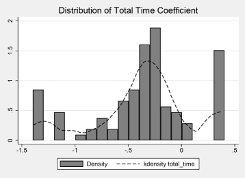
Figure 1: Distribution of Total Time Coefficient (Normal)

One solution to obtain non-positive estimates for the total_time coefficient is to use a bounded distribution. When using mixrandregret, we can specify that a coefficient is log-normally distributed for this purpose. In our case, since we want a non-positive distribution for the total_time coefficient, we have to multiply the total_time attribute for -1 to ensure that it is non-positive. To this end we create the new variable ntt, which corresponds to the negative of total_time.

• 
  

  . gen ntt = -1 * total_time
  
  . mixrandregret choice total_cost, group(cs) alt(altern) rand(ntt) ln(1) id(id) ///
  > nocons cluster(id) nrep(500) tech(bhhh) from(b_mixrrm)
  
  Iteration 0:   log likelihood = -994.35461
  Iteration 1:   log likelihood = -858.23241
  Iteration 2:   log likelihood =  -798.4694
  Iteration 3:   log likelihood = -785.66872
  Iteration 4:   log likelihood = -785.30817
  Iteration 5:   log likelihood = -785.27945
  Iteration 6:   log likelihood = -785.27728
  Iteration 7:   log likelihood = -785.27686
  Iteration 8:   log likelihood = -785.27675
  Iteration 9:   log likelihood = -785.27672
  Iteration 10:  log likelihood = -785.27671
  
  Case ID variable: cs                           Number of cases    =       1060
  Alternative variable: altern
  Random variable(s): ntt
  
                                   (Std. Err. adjusted for  106 clusters in id)
  
  Mixed random regret model                              Number of obs =   3,180
                                                         Wald chi2(2)  = 1230.55
  Log likelihood = -785.27671                            Prob > chi2   =  0.0000
  
                                                                                 
                                 OPG
        choice   Coefficient  std. err.      z    P>|z|     [95% conf. interval]
                                                                                 
  Mean          
    total_cost    -1.217682   .0442047   -27.55   0.000    -1.304321   -1.131042
           ntt    -1.312285   .1562202    -8.40   0.000    -1.618471   -1.006099
                                                                                 
  SD            
           ntt     1.363632   .1185994    11.50   0.000     1.131181    1.596082
                                                                                 
  
  The sign of the estimated standard deviations is irrelevant: interpret them as
  being positive
  
  

The estimated ntt parameters are the mean and standard deviation of the natural logarithm of the coefficient, and we can transform them back to the estimates of the coefficients themselves. The median of the coefficient is given by $\exp(b_{ntt})$, the mean is given by $\exp(b_{ntt}+s_{ntt}^{2}/2)$, and the standard deviation is given by $\exp(b_{ntt}+s_{ntt}^{2}/2)\times\sqrt{\exp(s_{ntt}^{2})-1}$ (Train, 2009). The sign change prior to the estimation is reversed by multiplying the estimates by -1.

• 
  

  . nlcom (mean_time: -1*exp([Mean]_b[ntt]+0.5*[SD]_b[ntt]^2))
  >       (med_time: -1*exp([Mean]_b[ntt]))
  >       (sd_time : exp([Mean]_b[ntt]+0.5*[SD]_b[ntt]^2)
  >                  *sqrt(exp([SD]_b[ntt]^2)-1))
  
     mean_time: -1*exp([Mean]_b[ntt]+0.5*[SD]_b[ntt]^2)
      med_time: -1*exp([Mean]_b[ntt])
       sd_time: exp([Mean]_b[ntt]+0.5*[SD]_b[ntt]^2)*sqrt(exp([SD]_b[ntt]^2)-1)
  
                                                                                 
        choice   Coefficient  Std. err.      z    P>|z|     [95% conf. interval]
                                                                                 
     mean_time     -.682127   .1587961    -4.30   0.000    -.9933616   -.3708923
      med_time    -.2692041   .0420551    -6.40   0.000    -.3516307   -.1867776
       sd_time     1.588122   .6295756     2.52   0.012     .3541763    2.822067
                                                                                 
  
  

Again, we calculate individual-level parameters. As we can observe in the listed data and distribution presented in Figure 2, all individual-level parameters are now negative as we expected.

• 
  

  . mixrbeta ntt, nrep(500) replace saving("${graphs_route}\mixRRM_ln_idl")
  
  . use "${graphs_route}\mixRRM_ln_idl" , replace
  
  . replace ntt = -1 * ntt /*reverse sign for graph*/
  (106 real changes made)
  
  . list id  ntt in 1/5
  
                              
         id          ntt  
                            
    1.    1   -.04032598  
    2.    2   -.08142616  
    3.    3   -.04047817  
    4.    4   -.04110615  
    5.    5   -.04025335  
                              
  
  

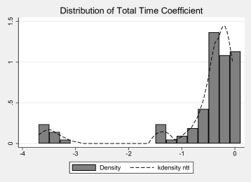
Figure 2: Distribution of Total Time Coefficient (Log-normal)

We can also generate predictions after running mixrandregret using mixrpred. To illustrate this command, we rerun the models using mixrandregret with normally distributed random coefficients, suppressing the output using the quietly command (see [U] quietly). Then, using the option proba, we generate the pred_p variable containing the predicted probability for each alternative. The code and output are listed below.

• 
  

  . qui mixrandregret choice total_cost, group(cs) alter(altern) rand(total_time) ///
  > id(id) nocons cluster(id) nrep(500) from(init_mix_rrm) tech(bhhh)
  
  . mixrpred pred_p, proba nrep(500)
  
  
  . list id cs altern total_time total_cost choice pred_p in 151/162, sepby(cs) ab(10) noo
  
                                                                          
      id   cs   altern   total_time   total_cost   choice     pred_p  
                                                                        
       6   51    First           23            6        0   .1516009  
       6   51   Second           27            4        1   .5547292  
       6   51    Third           35            3        0   .2936699  
                                                                        
       6   52    First           27            5        0   .3153724  
       6   52   Second           35            4        1    .291449  
       6   52    Third           23            6        0   .3931786  
                                                                        
       6   53    First           35            3        0   .3134595  
       6   53   Second           23            5        1   .5523607  
       6   53    Third           31            4        0   .1341798  
                                                                        
       6   54    First           27            4        0   .3153724  
       6   54   Second           23            5        1   .3931786  
       6   54    Third           35            3        0    .291449  
                                                                          
  
  

Additionally, mixrandregret also allows for the inclusion of ASC if users have labeled data. Although the data set is unlabeled in this example, we treat it as a labeled one in that each alternative represents a distinct category. We run the model including basealternative(1) option, which specify that the first alternative is the reference group for ASC.

• 
  

  . mixrandregret choice total_cost, group(cs) alt(altern) rand(total_time) id(id) ///
  > basealternative(1) cluster(id) nrep(500) tech(bhhh)
  
  Iteration 0:   log likelihood =  -1164.529
  Iteration 1:   log likelihood = -812.87881
  Iteration 2:   log likelihood = -773.05839
  Iteration 3:   log likelihood =  -769.1873
  Iteration 4:   log likelihood = -768.22193
  Iteration 5:   log likelihood = -767.97262
  Iteration 6:   log likelihood = -767.90237
  Iteration 7:   log likelihood =  -767.8867
  Iteration 8:   log likelihood = -767.88268
  Iteration 9:   log likelihood = -767.88165
  Iteration 10:  log likelihood = -767.88138
  Iteration 11:  log likelihood = -767.88131
  Iteration 12:  log likelihood = -767.88129
  
  Case ID variable: cs                           Number of cases    =       1060
  Alternative variable: altern
  Random variable(s): total_time
  
                                   (Std. Err. adjusted for  106 clusters in id)
  
  Mixed random regret model                               Number of obs =  3,180
                                                          Wald chi2(2)  = 465.50
  Log likelihood = -767.88129                             Prob > chi2   = 0.0000
  
                                                                                 
                                 OPG
        choice   Coefficient  std. err.      z    P>|z|     [95% conf. interval]
                                                                                 
  Mean          
    total_cost     -1.06784   .0498243   -21.43   0.000    -1.165494   -.9701866
    total_time    -.3455217   .0594409    -5.81   0.000    -.4620237   -.2290197
                                                                                 
  SD            
    total_time    -.5095087   .0420965   -12.10   0.000    -.5920163   -.4270012
                                                                                 
  ASC           
         ASC_2     .0064798   .0510223     0.13   0.899    -.0935221    .1064816
         ASC_3      .136445   .0605786     2.25   0.024     .0177131    .2551768
                                                                                 
  
  The sign of the estimated standard deviations is irrelevant: interpret them as
  being positive
  
  
  

7 Conclusions

This article presents the command mixrandrgret to fit Random Regret Minimization models with random parameters. We also developed the post-estimation command mixrpred for predicting the estimated probabilities. Additionally, the mixrbeta post-estimation command allows the user to estimate individual-level parameters for the random coefficients included in the model. The commands’ usage and options are illustrated using discrete choice data from van Cranenburgh and Chorus (2018).

8 Acknowledgments

We thank Michel Meulders, Jan De Spiegeleer, and the participants from the 2022 London Stata Conference for their helpful comments and constructive suggestions. Additionally, substantial portions of our programs were inspired by the book Maximum Likelihood Estimation with Stata, Fourth Edition by Willian Gould, Jeffrey Pitblado, and Brian Poi (2010). Finally, many of the previous checks to the data and the construction of the log-likelihood functions were greatly inspired by the randregret (Gutiérrez-Vargas et al., 2021) and mixlogit (Hole, 2007) commands.

9 Funding

This work was produced while Álvaro A. Gutiérrez-Vargas was a PhD student at the Research Centre for Operations Research and Statistics (ORSTAT) at KU Leuven funded by Bijzonder Onderzoeksfonds KU Leuven (Special Research Fund KU Leuven).

10 Conflict of interest

Ziyue Zhu, Álvaro A. Gutiérrez-Vargas, and Martina Vandebroek declare no conflicts of interest.

11 Contribution

Ziyue Zhu and Álvaro A. Gutiérrez-Vargas contributed equally to the article by developing the command and drafting the article. Martina Vandebroek critically commented on both the article and the command’s functionality.

About the authors

Ziyue Zhu is a master student of statistics and data science at KU Leuven in Belgium. She earned a Bachelor of Economics from Wuhan University and a Master of Economics from Barcelona School of Economics.

Álvaro A. Gutiérrez-Vargas is a PhD student at the Research Centre of Operation Research and Statistics (ORSTAT) at KU Leuven in Belgium. He earned a Bachelor of Science in economics from the University of Chile. His research interests are mainly methodological and focused on computational statistics, machine learning, and discrete choice models. He has been published in The Stata Journal and Journal of Choice Modelling.

Martina Vandebroek is a full professor at the Faculty of Economics and Business at KU Leuven in Belgium. She earned a PhD in actuarial sciences from KU Leuven. She is interested in the design of experiments, discrete choice experiments, and multivariate statistics. She has been published in Transportation Research B, Journal of Choice Modelling, Marketing Science, and Journal of Statistical Software, among other journals.

References

- Chorus (2010) Chorus, C. G. 2010. A new model of random regret minimization. European Journal of Transport and Infrastructure Research 10(2).
- Chorus (2014) . 2014. A generalized random regret minimization model. Transportation research part B: Methodological 68: 224–238.
- Chorus et al. (2008) Chorus, C. G., T. A. Arentze, and H. J. Timmermans. 2008. A random regret-minimization model of travel choice. Transportation Research Part B: Methodological 42(1): 1–18.
- van Cranenburgh and Chorus (2018) van Cranenburgh, S., and C. Chorus. 2018. Small value-of-time experiment, Netherlands [Data set]. TU Delft - 4TU.ResearchData .
- van Cranenburgh et al. (2015) van Cranenburgh, S., C. A. Guevara, and C. G. Chorus. 2015. New insights on random regret minimization models. Transportation Research Part A: Policy and Practice 74: 91–109.
- Gutiérrez-Vargas et al. (2021) Gutiérrez-Vargas, Á. A., M. Meulders, and M. Vandebroek. 2021. randregret: A command for fitting random regret minimization models using Stata. The Stata Journal 21(3): 626–658.
- Hensher et al. (2016) Hensher, D. A., W. H. Greene, and C. Q. Ho. 2016. Random regret minimization and random utility maximization in the presence of preference heterogeneity: an empirical contrast. Journal of Transportation Engineering 142(4): 1–10.
- Hole (2007) Hole, A. R. 2007. Fitting mixed logit models by using maximum simulated likelihood. The stata journal 7(3): 388–401.
- Loomes and Sugden (1982) Loomes, G., and R. Sugden. 1982. Regret theory: An alternative theory of rational choice under uncertainty. The economic journal 92(368): 805–824.
- McFadden (1974) McFadden, D. 1974. Conditional logit analysis of qualitative choice behavior. In: Zarembka, P., Ed., Frontiers in Econometrics, 105–142.
- McFadden and Train (2000) McFadden, D., and K. Train. 2000. Mixed MNL models for discrete response. Journal of Applied Econometrics 15(5): 447–470.
- Train (2009) Train, K. E. 2009. Discrete choice methods with simulation. Cambridge university press.
- Van Cranenburgh and Prato (2016) Van Cranenburgh, S., and C. G. Prato. 2016. On the robustness of random regret minimization modelling outcomes towards omitted attributes. Journal of choice modelling 18: 51–70.