Neural Point Catacaustics for Novel-View Synthesis of Reflections

Abstract.

View-dependent effects such as reflections pose a substantial challenge for image-based and neural rendering algorithms. Above all, curved reflectors are particularly hard, as they lead to highly non-linear reflection flows as the camera moves. We introduce a new point-based representation to compute Neural Point Catacaustics allowing novel-view synthesis of scenes with curved reflectors, from a set of casually-captured input photos. At the core of our method is a neural warp field that models catacaustic trajectories of reflections, so complex specular effects can be rendered using efficient point splatting in conjunction with a neural renderer. One of our key contributions is the explicit representation of reflections with a reflection point cloud  which is displaced by the neural warp field, and a primary point cloud  which is optimized to represent the rest of the scene. After a short manual annotation step, our approach allows interactive high-quality renderings of novel views with accurate reflection flow. Additionally, the explicit representation of reflection flow supports several forms of scene manipulation in captured scenes, such as reflection editing, cloning of specular objects, reflection tracking across views, and comfortable stereo viewing. We provide the source code and other supplemental material on https://repo-sam.inria.fr/fungraph/neural_catacaustics/

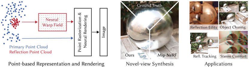
Figure 1. We propose a method to perform novel-view synthesis of curved reflectors. We employ a dynamic point-based scene representation that allows to model catacaustic trajectories of reflections for accurate reflection flow estimation. Our approach outperforms the state of the art in terms of image quality and supports a range of additional applications.

[TeaserFigure]TeaserFigure

1. Introduction

Recent neural rendering methods (Tewari et al., 2020, 2021) provide impressive visual quality for free-viewpoint rendering of captured scenes. Such scenes often contain important high-frequency view dependent effects, such as reflections from shiny objects, which can be modelled in two fundamentally different ways (Fig. 2): with an Eulerian approach where we consider a fixed representation of reflections and model directional variation in appearance, or via a Lagrangian solution where we track the flow of reflections as the observer moves. Most previous methods adopt the former by representing color on static points as a function of position and view direction using either expensive volumetric (Mildenhall et al., 2020; Wizadwongsa et al., 2021; Tewari et al., 2021), or mesh-based (Riegler and Koltun, 2021; Hedman et al., 2018) rendering. Instead, our solution directly learns reflection flow as a function of viewpoint via a Neural Warp Field, in effect adopting a Lagrangian approach (Bemana et al., 2020). Our point-based neural rendering method naturally allows reflection points  to be warped via the neural field, enabling interactive rendering.

Previous solutions often involve an inherent tradeoff between quality and speed, since to model (somewhat) high-frequency reflections they often use slow volumetric ray-marching with view-dependent queries. Fast approximate alternatives (Hedman et al., 2021; Yu et al., 2021) sacrifice angular resolution and thus reflection quality/sharpness. Overall, such methods use a multi-layer perceptron (MLP) to model density and view-dependent color parameterized by view direction, creating reflected geometry behind the reflector. Combined with volumetric ray-marching this often results in “foggy” appearance, lacking sharp detail in reflections. A recent solution (Verbin et al., 2021) improves the quality of such methods but still suffers from slow volumetric rendering. In addition, manipulating scenes with reflections is hard with such solutions.

Our Lagrangian, point-based approach avoids bias towards low frequencies inherent in implicit MLP-based neural radiance fields, which persists even when using different encodings and parameterizations. Our approach has two additional advantages: The overhead is lower during inference, allowing interactive rendering, and the direct representation makes scene manipulation easy.

We extract an initial point cloud using standard 3D reconstruction stereo from a multi-view dataset; after a minimal manual step to define a reflector mask on 3-4 images, we optimize two separate point clouds with additional high-dimensional features. During rendering, the primary point cloud is static, and represents the mostly diffuse scene component, while the second reflection point cloud represents highly view-dependent reflection effects; these latter points are displaced by the learned neural warp field  (see Fig. 1). Points also carry footprint and opacity parameters that are optimized with their position during training. The learned features of the two point clouds are then rasterized and interpreted by a neural renderer to produce the final image.

We are motivated by the theoretical foundation of geometric optics of curved reflectors, which shows that reflections from a curved object move on catacaustic surfaces (Lawrence, 2013; Hamilton, 1828); These often result in highly irregular, fast-moving reflection flows (Fig. 3). We train a flow field to learn these trajectories, which we call Neural Point Catacaustics, allowing interactive free-viewpoint neural rendering. Importantly, the explicit nature of our point-based representation facilitates manipulation of scenes with reflections, e.g., reflection editing, cloning of reflective objects, etc.

We first present the geometric background of complex reflection flow for curved reflectors that guides our algorithm, and then present the following contributions:

• A novel direct scene representation for neural rendering, with a separate reflection point cloud  displaced by a reflection neural warp field  that learns to compute Neural Point Catacaustics, and a primary point cloud  with optimized parameters to represent the rest of the scene content.

• A Neural Warp Field that learns the displacement of reflection points as a function of viewpoint. Stable training of our end-to-end method – including this field – requires careful parameterization and initialization, progressive training and point densification.

• Finally, we present a general, interactive neural rendering algorithm, that achieves high quality for both the diffuse and view-dependent radiance in a scene, allowing free-viewpoint navigation in captured scenes and interactive rendering.

We illustrate our method on several captured scenes, and show that it is quantitatively and qualitatively superior to previous neural rendering methods for reflections from curved objects, while allowing fast rendering and manipulation of such scenes: e.g., editing reflections, cloning reflective objects, or finding reflection correspondences in input images.

Figure 2. Eulerian vs. Lagrangian modeling of view-dependent effects. (a) A curved reflector is seen from two viewpoints. The reflection of a star appears at different positions with different distortions. (b) In the Eulerian approach, each surface point evaluates appearance as a function of view direction (black arrows). The red point is on in the left view, but is off in the right view. Reflections and their distortions must be learned for each surface point. (c) In a Lagrangian approach, reflected objects are represented once and their motion is modeled explicitly. Distortions naturally emerge from the motion of many reflection points.

2. Related Work

We review only closely related literature in traditional and image-based rendering of reflections – especially warping methods – and discuss neural rendering methods that use directional representations of radiance and also point-based (neural) rendering.

2.1. Rendering Reflections

Modeling and rendering reflections has been a major goal of Computer Graphics (CG) from its outset. Ray-tracing  (Whitted, 1979) directly simulated optics to render reflections, greatly enhancing realism of CG rendering. Initially, only simplified solutions such as environment or reflection mapping (Blinn and Newell, 1976) were practical.

Traditional Reflection Rendering.

Several solutions were initially proposed to render reflections with rasterization. For planar mirrors, a new virtual camera (Foley et al., 1996) and multi-pass rendering with virtual objects (Diefenbach and Badler, 1997) were used to render reflections, by rendering the reflected scene a second time. This idea was extended to curved reflectors (Ofek and Rappoport, 1998; Estalella et al., 2005) by deforming a virtual mesh to render reflected shapes, using different acceleration structures. Several solutions were subsequently proposed exploiting GPU shaders; see survey (Szirmay-Kalos et al., 2009). Similarly, we use points to represent reflection geometry, but we train a neural network to learn the flow of reflected points with viewpoint motion.

Glossy surfaces with varying levels of roughness can be treated by pre-filtering environment maps (Greene, 1986); this approach was extended by fast image-based warping of reflection probes  (Cabral et al., 1999). Path pertubation theory (Chen and Arvo, 2000) has been used to estimate displacement of specular paths; the same theory guided computation of probe-based reflection flow for ray-tracing (Rodriguez et al., 2020a). Lochmann et al. (2014) use an optimization to estimate reflection flow for distributed rendering. Our method has similar motivation to these methods, since we use reflection flow, but in the context of captured real scenes, which implies many additional challenges, e.g., inaccurate geometry.

Reflection Reconstruction and Image-Based Rendering with Reflections

3D reconstruction (Goesele et al., 2007) and image-based rendering (IBR) of scenes with reflections is notoriously difficult, since photoconsistency is violated. Several methods capture and render reflections using image-based approaches, typically by separating the input images into reflected and transmitted layers (Szeliski et al., 2000). Layer separation for reflections is a long-standing topic in computer vision with user-assisted solutions (Levin and Weiss, 2007), or recent deep learning methods based on polarization (e.g.,  (Wieschollek et al., 2018)). More sophisticated algorithms estimate reflected depth (Sinha et al., 2012) and allow efficient IBR (Kopf et al., 2013), but have difficulty with curved reflectors. A recent specific solution estimates curved reflector geometry for car windows, and performs ad-hoc layer separation to estimate reflection flow (Rodriguez et al., 2020b). In contrast, we present a solution that learns reflections on arbitrary curved reflectors.

Theoretically, geometry and material optimization using differentiable rendering (Nimier-David et al., 2019) could be used, but such solutions have not yet been demonstrated to work for captured scenes with incomplete geometry, especially in our case of shiny reflectors that have very incomplete reconstruction.

2.2. Neural and Point-Based Rendering

Neural Rendering is a vast and very fast-moving field; we thus only discuss research directly relevant to our work, i.e., reflection rendering/flow and point-based rendering; recent surveys (Tewari et al., 2020, 2021; Xie et al., 2021) cover the field in detail.

Several neural rendering methods propose specific treatment for reflections/specularities. Thies et al. (2019) use feature vectors in texture space to encode specular effects, but require dense angular sampling of input cameras. The X-fields method (Bemana et al., 2020) learns flow of various parameters – including specular reflections – but focuses on small-baseline “light-field like” camera motion. Our focus is on wide-baseline casual capture, and unconstrained free-viewpoint camera motion in full scenes.

NeX (Wizadwongsa et al., 2021) improves multi-plane image methods by learning a directional color representation as a linear combination of basis functions. Neural radiance fields (NeRF) (Mildenhall et al., 2020; Barron et al., 2021) learn density and view-dependent color using an MLP. NeRFs tend to create density corresponding to reflected objects behind the reflector, and use the view-dependent color term to simulate the desired appearance. This can represent reflection flow to a certain extent, but often fails to reconstruct sharp features and requires expensive volumetric rendering. The latter problem has been addressed in several variants (Garbin et al., 2021; Müller et al., 2022). In contrast to these representations, our explicit point-based method generally gives sharper results, and supports scene manipulation.

Other methods use the mesh provided by multi-view stereo reconstruction as a “scaffold”. Deep Blending (Hedman et al., 2018) uses view-dependent meshes for input image projection subsequently blended with learned weights; reflections blend in and out with simple interpolation, often creating severe temporal artifacts. Also, the per-input view data storage does not scale to datasets with large numbers of images. Recent work explicitly reconstructs the reflected image for planar reflections, using a superresolution neural network for rendering (Xu et al., 2021). Neural methods build view dependent deep features from input images merged onto this common space (Riegler and Koltun, 2021), while Philip et al. (2021) handle non-diffuse reflections explicitly, by providing mirror images to the neural renderer. All the above methods propose an Eulerian approach (Wu et al., 2012), since they store directional information in a fixed spatially-guided structure (explicit or implicit) as opposed to our Lagrangian estimation of reflection flow.

Recently published NeRF-based methods improve results for reflections, either by reparameterizing view-dependent color by the direction of reflection instead of view (Verbin et al., 2021), improving reflections for directional incoming lighting, or by learning a separate neural representation for planar reflections (Guo et al., 2021). Our method treats the general case of reflections on curved reflectors, and allows interactive rendering.

Finally, recent methods learn deformations using neural warp fields (e.g., (Park et al., 2021; Tretschk et al., 2021)), but for the different goal of handling dynamic content, while Wang et al. (2021) use a related idea to perform one-shot capture from an array of spherical mirrors. These methods can be considered Lagragian, but in a different context, i.e., for motion, or using reflections to reconstruct the non-specular scene.

Point-Based Neural Rendering

Point-based rendering is a flexible approach to rendering geometry (Gross and Pfister, 2007), since it does not require mesh connectivity. Points are typically splatted to the screen; choosing the size and shape of the splats must be done carefully (Zwicker et al., 2001). Interest in point-based rendering has been revived with the introduction of differentiable solutions (Wiles et al., 2020; Yifan et al., 2019), including fast approximations (Lassner and Zollhofer, 2021). Several neural rendering methods have been presented, directly rendering a point-based representation of the scene (Aliev et al., 2020)(Meshry et al., 2019), by projecting view-dependent features into the novel view (Kopanas et al., 2021), or in a fast rendering approach that optimizes camera parameters to improve quality (Rückert et al., 2022). In recent work, points are used to represent an implicit light field (Ost et al., 2021). Other methods use points as neural basis functions  (Xu et al., 2022) or local neural fields (Feng et al., 2022); both have mechanisms to upsample or grow the point cloud when necessary. Our method follows this line of work, exploiting the flexibility of points that are naturally adapted to the use of estimated reflection flow in our context, but also allow flexible representation for the rest of the scene, e.g., easy point densification when needed.

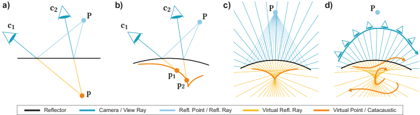
Figure 3. The geometry of catacaustics: (a) In the case of a planar reflector, a reflected point $\mathbf{P}$ results in a static virtual point $\mathbf{p}$, independent of camera position $\mathbf{c}$. (b) For curved reflectors (here a convex example), camera motion leads to $\mathbf{p}$ tracing a surface, called catacaustic. (c) The catacaustic for a single point $\mathbf{P}$ is defined by the envelope of virtual reflected rays, depicted as the bold orange curve, which at each point is tangent to one of the virtual reflected rays. Virtual images of $\mathbf{P}$ are formed only on the catacaustic trajectory. (d) In a point-based rendering setup, where the tangent constraint is not satisfied, the trajectory of virtual points is not unique. An infinite number of trajectories (three examples are shown) lead to the same apparent reflection. Reflection rays are omitted for clarity.

3. Background & Overview

Our goal is to develop a neural rendering method for scenes with reflectors, allowing interactive free-viewpoint rendering and scene manipulation. We next review the background on reflection geometry in this context, and present an overview of our method.

3.1. Geometry of Reflections from Curved Objects

For planar reflectors (Fig. 3a) the geometry is simple. Consider point $\mathbf{P}$; its reflection is a static virtual point $\mathbf{p}$ on the other side of the reflector, which does not move when the viewpoint changes. To obtain proper reflection flow during rendering, $\mathbf{p}$ just needs to be reprojected to the novel view (Foley et al., 1996; Xu et al., 2021; Guo et al., 2021).

For curved reflectors (Fig. 3b) things are more complex. Here, the position of the virtual point depends on the viewpoint, i.e., the point follows a trajectory in space as the view changes. The virtual points $\mathbf{p}$ trace a surface, which is called a catacaustic (Lawrence, 2013; Hamilton, 1828). The shape of the surface depends both on the position of the reflected point $\mathbf{P}$ and the shape of the reflector. The catacaustic surface is usually highly non-linear and has significantly higher complexity than the reflector geometry (Josse and Pene, 2014). Closed-form solutions exist for analytic reflector geometries. For example, a circular reflector results in a cardioid (Glaeser, 1999) and can be found with optimization for more complex shapes when exact geometry is available (Mitchell and Hanrahan, 1992). The catacaustic surface can lie behind or in front of the reflector surface, depending on $\mathbf{P}$ and whether the reflector is convex or concave, potentially resulting in large minifications and magnifications and other irregular motion.

In physics/geometric optics, given all geometric information, the position and shape of the catacaustic are uniquely defined: Only on the catacaustic surface, (virtual) optical images of $\mathbf{P}$ appear, since (virtual) reflected rays intersect only on these surfaces (Fig. 3c). For set of curves, the envelope is defined as a curve tangent to each one of the curves in the set. Specifically, the envelope is defined by these points of tangency (Bruce and Giblin, 1992). As catacaustics are the envelope of the virtual reflected rays (Hamilton, 1828) (Fig. 3(c)), the virtual points are only visible along the tangent ray of the catacaustic (also see Fig. 3b).

3.2. Neural Rendering of Reflection from Curved Objects

Free-viewpoint neural rendering of these moving reflections is complex. Our Lagrangian methodology estimates the catacaustic trajectories of the points reflected on curved reflectors, therefore storing reflections once and reusing them.

We learn reflection motion by training a Neural Warp Field (Sitzmann et al., 2019; Xie et al., 2021; Tewari et al., 2021) from multi-view images. This warp field is used to deform a virtual point cloud to match the reflections captured in the input views and, together with a neural rendering network, allow interactive free-view navigation in a scene with curved reflector shapes.

However, the use of points results in a deviation from physics: Since in point-based rendering a point emits light in all directions, it is a (virtual) optical image by construction, independent of its position. This means the trajectory of reflections is no longer unique (Fig. 3d): Any trajectory crossing virtual reflected rays in the correct order at the appropriate time results in the same apparent reflection as seen by a moving camera (modulo occlusions), resulting in a depth ambiguity. Recovering the physically correct catacaustic surface is not necessary for rendering since all the different solutions in Fig. 3d generate the same image.

Our method builds on the theory of catacaustic surfaces to learn the trajectories of reflection points, which we refer to as Neural Point Catacaustics. We perform an qualitative analysis comparing physical to neural point catacaustics in Sec. 7.7.

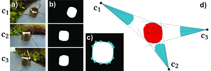
Figure 4. Bounding reflector volume: (a, b) The user is asked to paint rough masks marking the reflector in a small set (here 3) of images. (c) From these masks, we compute simple 2D bounding polylines (shown for $\mathbf{c_{2}}$ only). (d) Finally, we solve for the convex 3D polyhedron that satisfies all mask constraints.

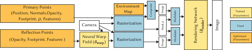
Figure 5. Overview of our method.

3.3. Method Overview

Our method takes multiple wide-baseline photos of a scene as input, typically 200-300 for a room or an outdoors scene, containing curved reflectors. We run standard structure-from-motion (SfM) to calibrate the cameras, and a standard multi-view stereo (MVS) method to extract a dense point cloud. A minimal manual step is then performed, where the user creates a coarse mask of the reflector(s) in 3-4 views in the dataset (this step typically takes less than 1 minute); these masks are used to extract a Reflection Volume  that encapsulates the reflectors.

Our method is illustrated in Fig. 5. The MVS reconstruction is used to initialize a primary point cloud, representing the diffuse and low-frequency view-dependent content of the scene. We also initialize a reflection point cloud  using the reflection volume created earlier. During training, we optimize the attributes of these two point clouds jointly.

To render an image given a free-viewpoint camera, we first displace the reflection point cloud  in 3D using a neural warp field, moving reflections to the correct position for a given camera. Then, both the primary  and the reflection point cloud  are rasterized separately using EWA splatting (Zwicker et al., 2001). The rasterized point clouds are composited together with an optimized environment map used to compensate for missing distant geometry. Finally, the resulting high-dimensional features are fed to a decoder neural renderer to synthesize the final image. Our architecture is trained end-to-end and results in an interactive free-viewpoint renderer.

4. Method

We now present the main components of our method, following Fig. 5 (left to right). We first discuss our dual point cloud representations, explain how the reflection points  are displaced by our Neural Warp Field, then discuss how we rasterize the points and their parameters, and finally discuss how we perform neural rendering.

4.1. Point Clouds

We use 3D points to represent the scene. In addition to their natural parameters i.e., positions and normal, we augment the points with additional parameters, all of which are optimized by our method. These properties allow the primary point cloud  to recover from incorrect and incomplete geometry from MVS reconstruction (see Fig. 7), and are central in learning the neural warp field  so that the reflection points  can be displaced to follow reflection flow.

The parameters we optimize for all points in both clouds are: opacity, footprint and high-dimensional features. For primary points  we also optimize position, normals and parameter $\rho$ that will be used to modulate rasterized point clouds.

4.2. Neural Warp Field

We define a neural warp field  which is responsible for displacing reflection points  with camera motion. Formally, given an initial reflection point  position $\mathbf{p}\in\mathds{R}^{3}$ and the current camera position $\mathbf{c}\in\mathds{R}^{3}$, we seek to compute the reflection position $\mathbf{p^{\prime}}\in\mathds{R}^{3}$ on the Neural Point Catacaustic, using the field $\mathcal{F}\in\left(\mathds{R}^{3}\times\mathds{R}^{3}\right)\rightarrow\mathds{R}^{3}$ via:

$$\mathbf{p^{\prime}}=\mathbf{p}+\mathcal{F}(\mathbf{p},\mathbf{c}).$$

We realize $\mathcal{F}$ using an MLP with trainable parameters $\theta_{\text{warp}}$. The initial point positions $\mathbf{p}$ are fixed, not optimized (see Sec. 5.1 for our initialization procedure), but each point is displaced by the neural warp field. Notice that the warp field takes the initial point position $\mathbf{p}$ as input, so that we can use the same field for all reflection points, resulting in a compact representation of the entire reflection flow.

4.3. Rasterization

We use differentiable point splatting (Yifan et al., 2019; Kopanas et al., 2021) to rasterize our point clouds. Each point can be seen as an oriented disk with position $\mathbf{p}$ and a normal, projected onto the screen as a soft ellipsoid. Each point also has a 3D footprint, defined as the squared radius of the disk, a 6-channel neural feature, and an opacity $o$.

The primary point cloud  is tasked to represent the geometry of the scene. We learn an additional parameter $\rho$ for each primary point; This scalar value will later control how much of the reflection point cloud  is blended in the final rendering.

To rasterize a point, we need to determine its 2D footprint, respecting the distance to the camera and its slant as defined by the point normal. To this end, we compute the covariance matrix for each point as follows (Zwicker et al., 2001; Ren et al., 2002):

(1) $$\Sigma~{}=~{}h^{2}\mathbf{J}\mathbf{V}{\mathbf{J}}^{T}+~{}\nu\mathbf{I}$$

where $\mathbf{J}\in\mathds{R}^{2\times 2}$ is the Jacobian of the transformation from world space to view space, $h$ is a scaling factor accounting for pixel resolution (Zwicker et al., 2001), and $\mathbf{V}$ is the identity matrix scaled by the 3D footprint of the point. $\nu\mathbf{I}$ is a low-pass filter; we use $\nu~{}=~{}0.3$ for all our tests, striking a balance between gradient instability arising from aliasing, and recovering high-frequency features.

We perform front-to-back compositing of all the splats to compute a pixel feature value $c$. We follow previous work (Yifan et al., 2019; Kopanas et al., 2021) and compute for all points $\mathcal{N}$ that fall on a pixel:

(2) $$c=\sum_{i\in\mathcal{N}}c_{i}\alpha_{i}\prod_{j=1}^{i-1}(1-\alpha_{j}).$$

Our $\alpha_{i}$ is given by evaluating a 2D Gaussian with covariance $\Sigma$ (Eq. 1) (Yifan et al., 2019) and multiplying it with the learned per-point opacity parameter $o$. The opacity value $o$ permits the optimization to make points “disappear” which allows to correct for erroneous overreconstruction from MVS. We call the full product:

(3) $$\bar{o}~{}=~{}\prod_{j\in\mathcal{N}}(1-\alpha_{j})$$

accumulated opacity, to be used in a loss described in Sec. 5.2 and for the environment map described below.

We use an environment map for the cases where MVS did not manage to compute geometry; this happens for objects far away, viewed from only a few views in large scenes. We parameterize an environment map with polar coordinates and we initialize with 6 features with a constant value of zero. During rendering, we project the environment map to the view and blend it using accumulated opacity $\bar{o}$.

Final	Primary Points
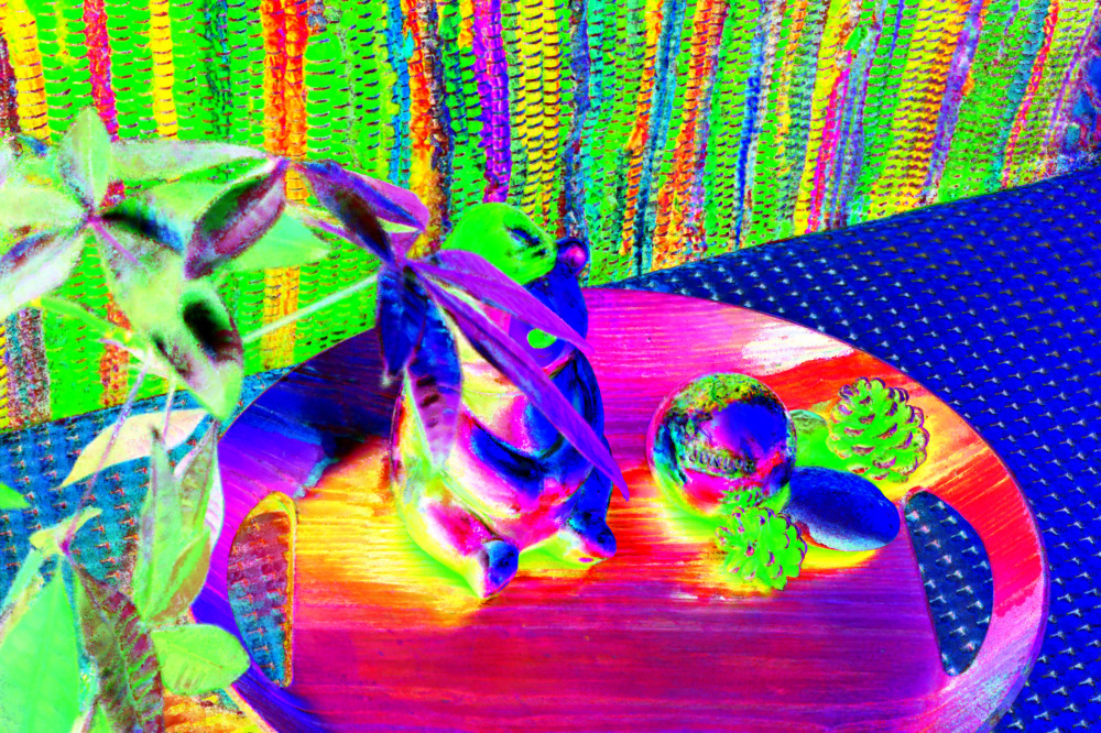
Reflection Points	$\rho$ Mask

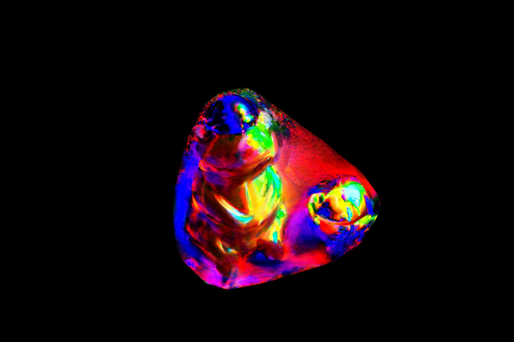
Figure 6. Intermediate buffers provided to the neural rendering network. For the primary and reflection point clouds we show the first three channels as RGB. Notice how the primary point cloud captures the non-specular appearence of the objects i.e., the texture on the porcelain bear, while the reflection point cloud captures all the specular details. The mask $\rho$ handles occlusions between specular and non-specular objects.

4.4. Neural Rendering

Once we have rasterized and composited all points and their corresponding parameters, i.e., 6-channel features and $\rho$, we feed this information into a neural renderer MLP with two heads. The first head encodes rasterized features of the primary points  plus the view direction into a latent feature. Feeding the view direction allows the primary point cloud to model low-frequency view-dependent effects (Eulerian-style), which almost all real-world materials exhibit to some extent.

We use a mask $\rho$ to modulate these primary rasterized features. The second head does the same for the reflection point  features independently, and is modulated by $1-\rho$. We concatenate the outputs of the two branches and feed them into a decoder network to obtain the final image. All the layers used by the renderer are illustrated in Fig. 6. We denote the trainable parameters of this module $\theta_{\text{render}}$.

5. Optimization and Training

Recall we have two point clouds, one for reflections and one for the remaining scene content; we optimize the parameters of these two point clouds and the two networks jointly. This joint optimization process poses several significant challenges, especially for the reflection flow that models complex motion and thus is prone to instabilities which we address with our method. We discuss how to initialize and regularize reflection points  and their motion in space using a reflection volume, created with minimal user intervention. We then discuss our loss function and our optimization using a multi-resolution solver and point densification.

5.1. Initializing and Regularizing Reflection Points

In many scenes, reflective surfaces tend to be restricted in space; Our test scenes each contain one main curved reflector, and the input photos include views around the object to ensure good angular coverage of reflections and view of the entire scene for free-viewpoint rendering. We consider the 3D volume that contains the reflective object(s). This reflection volume  represents the approximate region in space where we expect our Neural Point Catacaustics to move. We initialize the reflection point cloud  by randomly placing points on the bounding surface of the reflection volume. We use 400K points in all our experiments. The initialization on a 2D surface is a natural choice, since the scene elements we see in the reflections mostly consist of (or can be approximated by) surfaces. Additionally, we will use the reflection volume  to regularize the warped position of the reflection point cloud  during the optimization (Sec. 5.2).

We define the reflection volume by identifying the regions corresponding to reflection objects in the input images. Methods for automatic detection of reflections exist (Whelan et al., 2018), but have not yet been shown to robustly handle curved reflectors. Therefore, we opt for an approach with minimal user intervention: The user is asked to paint rough masks in a small number of input images, marking the objects with reflections (Fig. 4a and b). We use three or four images in all our examples; Painting takes less than a minute for a given dataset.

From these masks, and the 3D calibration of the corresponding cameras, we compute a convex polyhedron bounding the 3D space occupied by the reflector in three steps. First, we compute the convex hull of each 2D mask and simplify it using the Douglas-Peucker (1973) algorithm. The result is a closed polyline $L_{i}$ per image $i$ (Fig. 4c). We then lift everything to 3D: Using information from the calibrated cameras $\mathbf{c}_{i}$, we can associate each vertex of $L_{i}$ with a corresponding 3D point on $\mathbf{c}_{i}$’s image plane. Together with the camera’s center of projection, each two adjacent vertices define a plane (blue triangle fans in Fig. 4d), each separating 3D space into two half spaces; one contains the reflector, the other does not. Finally, we solve for the convex polyhedron which bounds the 3D space where all constraints are fulfilled (Preparata and Shamos, 1985) (red shape in Fig. 4d).

5.2. Loss

Our architecture is trained end-to-end for each specific scene – which is standard practice for recent neural rendering methods  (Mildenhall et al., 2020; Tewari et al., 2021; Kopanas et al., 2021).

Our loss consists of five terms:

(4) $$\mathcal{L}=\lambda_{\ell_{1}}\mathcal{L}_{\ell_{1}}+\lambda_{\textrm{DSSIM}}\mathcal{L}_{\textrm{DSSIM}}+\lambda_{\mathbf{p}}\mathcal{L}_{\mathbf{p}}+\lambda_{m}\mathcal{L}_{m}+\lambda_{m_{TV}}\mathcal{L}_{m_{TV}}.$$

$\mathcal{L}_{\ell_{1}}$ and $\mathcal{L}_{\textrm{DSSIM}}$ penalize differences between the output of the neural renderer and the corresponding input view in terms of $\ell_{1}$-norm and the DSSIM metric (Loza et al., 2006), respectively. $\mathcal{L}_{\mathbf{p}}$ encourages the reflection points  to stay within the reflection volume. For this, we use a binary mask $m_{\mathrm{RV}}$ created by projecting the reflection volume  into the current view. We take the (soft) accumulated opacity $\bar{o}$ (Eq. 3) of the reflection points  and compute

(5) $$\mathcal{L}_{\mathbf{p}}~{}=~{}\|(\bar{o}~{}-~{}m_{\mathrm{RV}})m_{\mathrm{RV}}\|_{1}.$$

For points that lie outside the projection of the reflection volume, this term has no effect, allowing some freedom for points to move outside the volume, but encourages points to stay inside to “fill” the reflector surface. $\mathcal{L}_{m}$ and $\mathcal{L}_{m_{TV}}$ regularize the rasterized mask $\rho$. $\mathcal{L}_{m}$ compares it to the binary mask $m_{\mathrm{RV}}$ in terms of the $\ell_{1}$-norm, encouraging the mask to light up for the reflector. Finally, $\mathcal{L}_{m_{TV}}$ encourages smoothness of $\rho$ by penalizing its total variation. An example of the $\rho$ mask is shown in Fig. 6.

We use an ADAM optimizer and weight decay for $\theta_{\text{warp}}$ for all our scenes, and we employ learning rate scheduling. The values of the parameters are $\lambda_{\ell_{1}}=0.05,~{}\lambda_{\text{DSSIM}}=0.2,\lambda_{\mathbf{p}}=\lambda_{m}=0.01,~{}~{}\lambda_{m_{TV}}=1e-5$.

5.3. Progressive Optimization

We optimize point parameters and the neural networks end-to-end by rendering patches of the input views. In each iteration, we render a random 150x150 pixel patch from a random input view and compute the loss given a ground truth image. We back-propagate the gradients every 20 iterations, in a manner equivalent to batches to avoid memory saturation.

If done naively, the early stages of the optimization can be unstable; the process may collapse to a degenerate case i.e., moving the reflection point cloud  outside the camera frustum. To avoid this, we use multi-resolution optimization. We also progressively densify the primary point cloud  to recover from large errors of MVS while maintaining sufficient point density.

The multi-resolution approach starts the optimization at low resolution, i.e., with downsampled images and reduced point-clouds by taking one out of every 32 points at the outset. By operating on smaller images, and thus larger image regions, the method provides a stable initialization for the opacity and 6-channel features of the points. In a short warm-up phase we upsample twice, each time doubling resolution and retrieving progressively more of the original points. At the end of the the warm-up, we reach full image resolution and original point cloud size, and we then start optimizing all parameters. We visualize the evolution of the optimization over time in Fig. 7.

MVS reconstruction can fail in some parts of the scene, creating empty regions of space. This has the consequence that points may move towards these empty regions, resulting in a sparse point cloud. To overcome this problem, we densify the point cloud every 2K iterations: For points with high view-space positional gradients we spawn a new point along the gradient direction.

Step: 2,000 -2min-	Step: 50,000 -3h 25min-
Step: 100,000 -8h 47min-	Step: 200,000 -22h 5min-

Figure 7. The final rendering throughout the optimization process. On the top left we show the image before the warm up finishes. On the top right, we can see that the quality is greatly improved, but the full reconstruction of the specular sphere is still missing. And on the bottom right we have reconstructed the full sphere.

6. Implementation

We next present details of our implementation for the rasterization, neural network and our interactive renderer. All renderings for optimization and for all results were performed at resolution 1000x666. All source code and data are available here: https://repo-sam.inria.fr/fungraph/neural_catacaustics/

6.1. Capture

We take a few hundred photographs of a given scene focusing on an central reflective object. The photos are then calibrated using off-the-sheld Structure-from-Motion (SfM) and we generate a dense point cloud using Multi-View Stereo (Reality, 2018), used to initialize the primary point cloud. We use RealityCapture in our experiments, which takes 5-8min for SfM and 30-40min for MVS on all our scenes on our Intel Xeon 5118 Gold PC.

6.2. Rasterization for Training

We implement our method in Pytorch using custom CUDA kernels (inspired by  (Yifan et al., 2019; Kopanas et al., 2021)). While front-to-back compositing of points is trivially differentiable, the computation of rasterized feature gradients with respect to point position and footprint has quadratic complexity in the number of points per pixel when implemented naively. Different from recent previous work (Lassner and Zollhofer, 2021), which only use a small subset of rasterized points in their backward pass, we use all rasterized points to obtain stable gradients. As a remedy, we implemented a custom two-pass recursive strategy (front-to-back followed by back-to-front) to yield exact gradients while reducing time complexity to linear.

6.3. Network Details

The warping field is an MLP with ReLU activations of 4 layers and 256 features. We carefully normalize the camera position and the reflection point cloud  to the range $[-1,1]$ and we scale down the output by of this network by multiplying with 0.01 to enforce a very small magnitude of the displacements when the optimization starts.

Our environment maps have a resolution of $1000\times 400$. The Neural Renderer is an MLP with ReLU activations: both encoders and the decoder share the same architecture and have 32 features and 9 layers. For every 2 layers, we have a residual connection. We initialize them with FixUp. We opted for an MLP instead of CNNs that have been used in previous work (Kopanas et al., 2021; Philip et al., 2021). While CNNs naturally provide high-quality renderings, they suffer from temporal artifacts due to screen-space filtering. In addition, initial tests showed that for our end-to-end optimization, the ability of the CNN to correct artifacts in screen space undermines the ability to recover an accurate 3D scene representation.

6.4. Interactive Rendering

We observed that the main bottleneck of our pipeline is the rasterization of the primary point cloud, preventing interactive rendering. As a remedy, we have implemented an interactive OpenGL-based framework, which approximates the rasterization with hardware-accelerated EWA surface splatting (Ren et al., 2002). We use visibility splatting with depth peeling to create three semi-transparent render layers, which are composited to form the final feature tensor. Rasterization takes 100 ms, and in conjunction with the unoptimized Python-based Pytorch implementation of the remaining parts of the pipeline, we achieve 5 fps. We analyze the resulting image quality in Sec. 7.3.

Figure 8. Results of our method on Compost, ConcaveBowl, HallwayLamp, SilverVase: left is our rendering, right is the ground truth from images not in the input views. Note how our renderings faithfully capture reflections.

7. Results & Evaluation

We first present results of our method, then discuss applications to different manipulations of reflections, and finally present quantitative and qualitative evaluations.

We captured 5 scenes for evaluation: one outdoors scene, Compost, and four indoors scenes, SilverVase, HallwayLamp, ConcaveBowl, and CrazyBlade. The last two contain concave reflectors. Since we model motion of reflections, our results are best appreciated in video paths; we provide these for all scenes and comparisons in the supplemental.

7.1. Results

We optimize our end-to-end model for approximately 36 hours on a single RTX8000 GPU for each scene. We show results compared to ground truth images from paths away from the input views in Fig. 8. Our method recovers and renders sharp reflections which move smoothly (please see supplemental videos), even for complex cases such as the concave reflectors in CrazyBlade and ConcaveBowl. Overall, the shape, position and motion of the reflections is close to the ground truth.

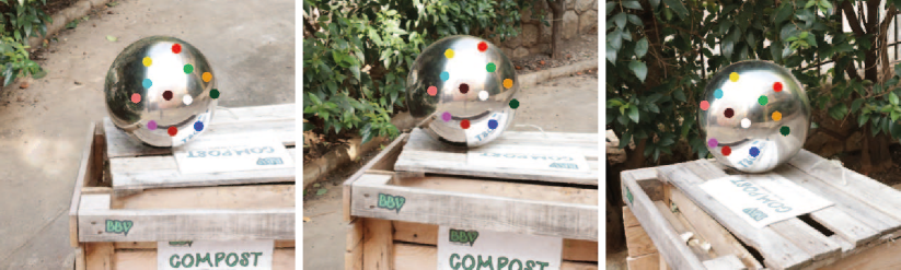
Figure 9. Our neural warpfield formulation naturally establishes correspondences of reflections across views, allowing to track reflections also in the presence of severe deformations. Example correspondences are marked as colored dots; please also refer to the supplemental video.

7.2. Applications

Besides novel-view synthesis, our approach naturally enables a wider range of applications:

7.2.1. Correspondences in reflections

A powerful consequence of our Lagrangian design is direct support for dense correspondences in non-rigidly deforming reflections across views. In Fig. 9 we show how reflection points are faithfully tracked across different views, by following the projected learned trajectories of virtual reflection points as defined by our neural catacaustic field. We envision downstream applications like specular surface reconstruction (Roth and Black, 2006; Sankaranarayanan et al., 2010) and view-coherent image annotations (Caelles et al., 2017) of reflected objects to greatly benefit from these dense correspondences.

7.2.2. Scene and reflection editing

In addition to physical correctness, some rendering applications also need to consider artistic goals. Reflections are particularly amenable to artistic modification for their ability to convey spatial relations, while human observers are tolerant to deviations from physical correctness (Ramanarayanan et al., 2007). Tools for reflection editing have been developed for synthetic scenes (Ritschel et al., 2009; Schmidt et al., 2013). Even though our pipeline is trained to faithfully reproduce input views, after training our approach allows expressive editing of reflections by decoupling the camera used for rasterization from the camera that is fed to the neural catacaustic field responsible for warping the reflections. This way we can move reflections in a way that is coherent both spatially and across views, enabling believable edits of reflected perspective (Fig. 10, and supplemental video).

Further, our explicit scene representation supports general editing. In Fig. 11 we show an object cloning example. To achieve this result, we copy the primary points  contained in the volume we wish to clone, and transform them. We then replicate the reflection point cloud  and apply the inverse transformation to the camera used to warp the reflection points. Note that we can only perform translations of the cloned objects for now; rotations would probably require specific training or parameterization.

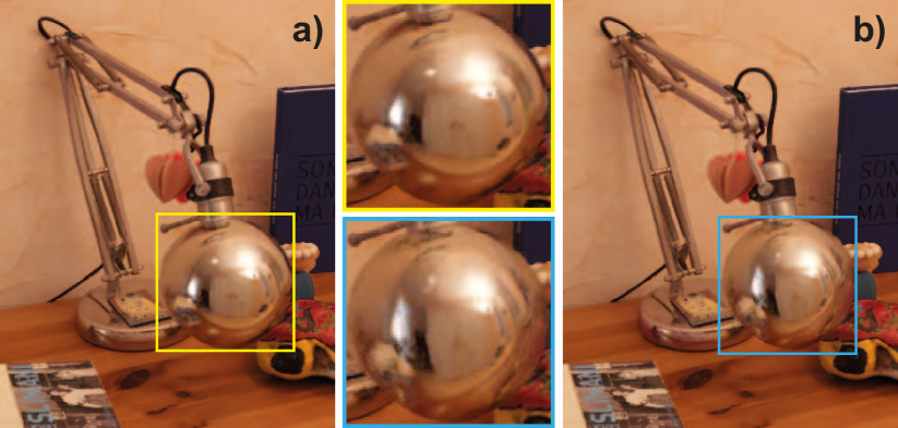
Figure 10. Reflection editing. (a) Original rendering. (b) Edited reflection, magnifying the right part of the table. The edited reflections correspond to a camera to the left of the primary view camera.

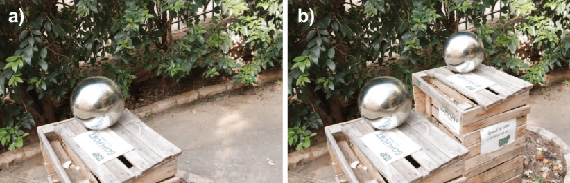
Figure 11. Our explicit scene representation allows versatile editing. (a) Original scene. (b) Cloning of the reflection point cloud  as well as part of the primary point cloud. The reflections on the two spheres are different, resulting in plausible perspective across novel views (see supplemental video).

7.2.3. Comfortable stereo

Stereoscopic rendering of reflections, e.g., for VR applications, is challenging – especially for curved reflectors, where excessive horizontal and vertical disparities can occur, significantly impairing viewing comfort (Lambooij et al., 2009; Shibata et al., 2011). While solutions exist to enforce a comfortable disparity range for diffuse appearance (Jones et al., 2001; Lang et al., 2010), the corresponding problem for specular surfaces has only been addressed for synthetic scenes with full control over the image generation process (Dabała et al., 2014; Templin et al., 2012).

Our approach enables control over binocular disparity arising from curved reflectors in casually captured scenes. Again, we exploit that we can decouple the stereo cameras used for rasterization from the stereo cameras steering the warpfield: We simply decrease the inter-ocular distance between the latter stereo cameras in case of uncomfortably large binocular disparities (Fig. 12). In the limit of a single (cyclopean) camera as input to the catacaustic field, reflections for both eyes lie at the same point on the learned catacaustic, resulting in stereo characteristics of a diffuse scene element with an offset from the reflector surface (Templin et al., 2012), preventing visual discomfort. Notice that the diffuse (primary) rendering branch of our pipeline is not affected by this modification.

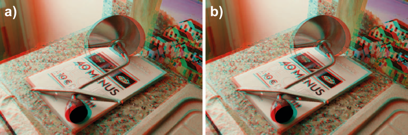
Figure 12. Our method supports comfortable stereo rendering of reflections. (a) Curved reflectors frequently result in uncomfortable binocular disparities (most prominent at the top left of the blade). (b) Our approach allows for an explicit modification of disparities, preventing visual discomfort. Use anaglyph glasses for stereo impression.

7.3. Evaluation

We evaluate our approach qualitatively and quantitatively in terms of rendering quality. We first show comparisons to previous work and then present ablations evaluating the tradeoffs of our different choices.

For our quantitative tests, in addition to our input views, we captured a high-speed sequence of photographs using the same settings, which gives paths of about 10-15 fps. We thus have ground truth sequences of images that are completely distinct from the input views for quantitative evaluation. Since we want to evaluate the quality of our renderings of reflections, we compute all image metrics in the region of the image covered by the project of the reflection volume. All paths and renderings of all methods for these quantitative evaluations are provided in supplemental material. We have selected subsequences of these paths and provide high fps interpolation to better evaluate reflection quality and motion, also presented in the supplemental.

We also show the effect on quality of our unoptimized interactive renderer that runs 5 fps in Fig. 13.

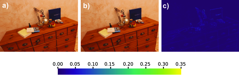
Figure 13. (a) Full renderer. (b) Interactive renderer, running at 5 fps in our unoptimized Python implementation. (c) Absolute normalized difference between a) and b).

7.4. Comparisons

We compare to MipNeRF (Barron et al., 2021) which is the current state-of-art NeRF method with code available , and to three interactive methods: Deep Blending (Hedman et al., 2018), the Point-Based Neural Rendering (PBNR) method of Kopanas et al. (2021), and Instant Neural Graphics Primitives (Müller et al., 2022). All methods were trained with the same resolution images (1000x666). We trained MipNeRf for 1M iterations with the default batch size, for approximately 48 hours. We compare all renderings with our full unoptimized method, currently running at 1.5s/frame.

GT	Ours	(Hedman et al., 2018)	(Müller et al., 2022)	(Barron et al., 2021)	(Kopanas et al., 2021)

Figure 14. We show comparisons to previous methods and the corresponding ground truth images from paths not in the input views. The scenes are, from the top down: HallwayLamp, SilverVase, CrazyBlade, Compost, ConcaveBowl.

Fig. 14 shows qualitative comparisons of our method to previous work and the ground truth. We see that our method renders sharper and more accurate reflections in the majority of cases. Surprisingly, Deep Blending performs very well; however, it is prone to catastrophic failure for some views (see ConcaveBowl in Fig. 14, where our method has recovered the missing geometry). Deep Blending also does not scale with the number of images: GPU memory requirements grow with the number of images – 300 images is about the limit of what current GPUs can handle for this method. In contrast our approach uses approximately the same amount GPU memory for any scene (around 8Gb). Deep Blending and PBNR suffer from severe flickering and temporal artifacts in some scenes; please see Compost and ConcaveBowl in supplemental.

In Tab. 1 we show quantitative results for all methods averaged over all scenes. The error is computed on views not in the input views, on paths that are distinct from those used for capture. We compute D-SSIM, PSNR and L-PIPS error; our method has the best quantitative results compared to all other methods, although we are only marginally better than Deep Blending, which however has severe temporal artifacts not captured by these metrics (please see video).

Table 1. Quantitative evaluation of our method compared to previous work, computed over our five scenes, on separate paths captured specifically for evalution, and separate from the input views.

	$SSIM^{\uparrow}$	$PSNR^{\uparrow}$	$LPIPS^{\downarrow}$
MipNeRF (Barron et al., 2021)	0.9772	34.6753	0.0258
InstantNGP (Müller et al., 2022)	0.9769	34.3459	0.0253
Point-Based NR (Kopanas et al., 2021)	0.9790	34.3463	0.0229
Deep Blending (Hedman et al., 2018)	0.9832	35.6316	0.0197
Ours	0.9845	35.8522	0.0179

7.5. Ablations

We also executed an ablation study to better understand the dynamics and the influence of several components in our system. Our experiments consist of runs on Compost for 200k iterations (0.5 - 1 day). The different elements of the ablation are: i) Primary-Only, where we render the scene only with the primary point cloud; ii) No-Densification, where we do not densify the original point cloud we get from MVS. iii) No-$\mathcal{L}_{\textrm{DSSIM}}$ and No-$\mathcal{L}_{m_{TV}}$, where we zero out these two loss terms. iv) Half-Warp-MLP, where we cut down the number of parameters of our warping field MLP in half.

Table 2. Quantitative effect of our ablation study for the different components of our algorithm, using the same methodology as Tab. 1.

	$SSIM^{\uparrow}$	$PSNR^{\uparrow}$	$LPIPS^{\downarrow}$
Primary-Only	0.9689	32.0426	0.0303
No-Densification	0.9727	32.6982	0.0273
No-$\mathcal{L}_{\textrm{DSSIM}}/\mathcal{L}_{m_{TV}}$	0.9704	33.2101	0.0284
Half-Warp-MLP	0.9690	32.5671	0.0301
Full	0.9745	33.7041	0.0254

As we can see in Tab. 2 and Fig. 15,16, each component of our method improves the results, in particular the importance of the neural warp field  is clear, as well as the densification and the MLP capacity. Primary-Only and Half-Warp-MLP cannot recover the movement of reflections and result in blurrier renderings. The No-Densification configuration struggles to recover from large errors in the reconstructions of the geometry during MVS. Another interesting finding of our ablation is that the two loss terms $\mathcal{L}_{\textrm{DSSIM}}$ and $\mathcal{L}_{m_{TV}}$ to a large extend remove the photographer from the reflections. This also has an effect on the numerical results in Tab.2, since the No-$\mathcal{L}_{\textrm{DSSIM}}/\mathcal{L}_{m_{TV}}$ configuration actually removes the photographer less, resulting in a bias with respect to the ground truth. Depending on the application, this might or might not be desirable.

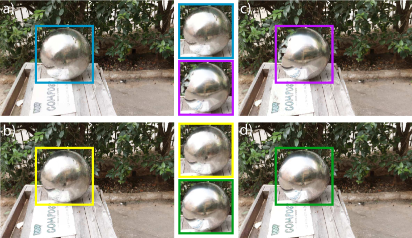
Figure 15. We show the effect of the various components of our methods on the results by ablation runs. a) Primary-only, b) Half-Warp-MLP, c) No-Densification, d) Full Method.

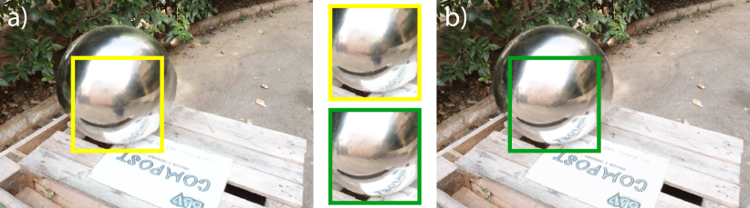
Figure 16. $\mathcal{L}_{\textrm{DSSIM}}$ and $\mathcal{L}_{m_{TV}}$ have the surprising effect of removing the photographer from the reflections.

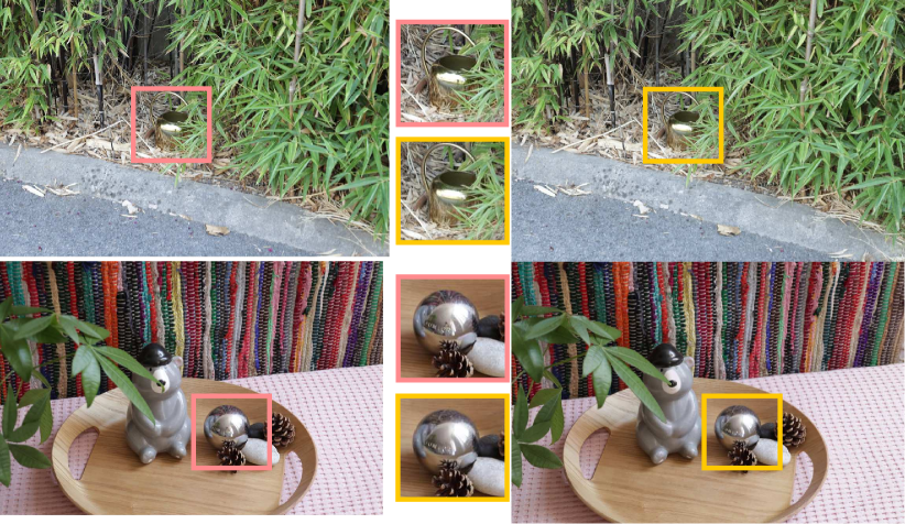
Figure 17. Two scenes illustrating how our method handles occlusions of reflectors by the non-specular scene (vegetation in front of watering can in the first row), and handles multiple reflections (note the reflection on the bear in the reflections of the sphere in the second row).

7.6. Occlusion, Texture and Multi-Bounce Reflections

Our method handles occlusion from diffuse objects, reflectors with texture and multi-bounce reflections. To illustrate this, we provide two scenes specifically captured for this purpose, shown in Fig. 17.

When a diffuse object occludes a reflector, the primary point cloud can reason about the occlusion because it contains both the reflector and the diffuse occluder. This information then propagates through the pipeline to the mask $\rho$. Specifically, in regions where the diffuse occluder is in front of the specular point cloud $\rho$ is $0$ and thus the specular point cloud will not be rendered. This can be seen in Fig. 6; example renderings are shown in Fig. 17 (first row and insets).

Specular reflectors (e.g., plastic or porcelain) can have diffuse texture. Our pipeline can model both in the separate point clouds and blends them using the value or $\rho$, correctly preserving the texture. We see this in Fig. 17 (second row), where reflections are correctly rendered despite the painted parts on the porcelain bear. However, we expect quality to degrade with more high frequency texture.

Multiple specular objects with multi-bounce specular effects often appear together; they can be treated as one specular point cloud if they are close (e.g., for the lamp base and lampshade in Hallway). For multiple reflector objects far apart, multiple specular point clouds should be used.

Since we do not explicitly model physical light transport, higher order reflections and global illumination do not become exponentially more complex as scene complexity increases. Such reflections are just a more complicated motion that the warp-field MLP needs to extract from the observations in the input images. We see this in Fig. 17 (second row and insets), where the reflections on the bear are visible in the reflections of the sphere.

7.7. Comparison to Physical Catacaustics

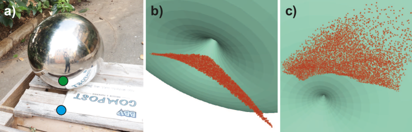
Figure 18. Comparing neural point catacaustics to physical catacaustics. (a) We consider a spherical reflector, for which an analytic catacaustic surface exists. (b,c) Two views of the geometric configuration. The cyan mesh represents the ground truth catacaustic surface of the blue point in a). The red points are samples from our learned neural point catacaustics of the green point in a). Please also refer to the main text.

There is no unique correct neural point catacaustic for a specific reflection due to the inherent depth ambiguity arising from our point-based representation (Sec. 3; Fig. 3d). Our system finds a solution that results in high-quality view-coherent renderings. Nevertheless, we are interested in a qualitative analysis of the emerging catacaustic geometry. To this end, we consider a scene with a known spherical reflector (Fig. 18a) and a reflected point with known position (blue point in Fig. 18a) and compute its analytic catacaustic surface (cyan mesh in Fig. 18b and c) (Glaeser, 1999). Then, we randomly sample the volume of camera positions from which the corresponding reflection (green point in Fig. 18a) is visible, and record the output of our warp field for the corresponding specular point (red points in Fig. 18b and c). While the two solutions roughly share some qualitative characteristics, they are quite dissimilar, despite resulting in almost identical projected reflection flow.

8. Discussion & Conclusion

Our solution produces renderings of curved objects that are of higher visual quality and quantitatively better than all previous methods; our explicit representation of the reflection point cloud  has the additional advantage of enabling several kinds of scene manipulations, such as reflection editing, reflector cloning, comfortable stereo rendering and dense reflection tracking across views.

Nonetheless, our approach is not without limitations. We have currently tested on scenes where the reflector only covers a small part of the scene; we expect our method to work relatively well as long as SfM/MVS can produce a reasonable first approximation of the scene, but there will most probably be new issues to be dealt with.

The focus of our work is on curved reflectors. Flat surfaces are a special case (Fig. 3(a)); we simply need to move specular points to their unique static positions. Our method would in principle be able to handle these cases, but would require adjusting our initialization to avoid excessive motion magnitudes. Depth ambiguity (Fig.  3(d)) gives our warp field a lot of freedom in choosing point trajectories without sacrificing reflection quality. This tends to favor short and simple trajectories (Fig. 18).

Our Lagrangian model assumes that view-dependent effects can be modeled by moving reflections. This assumption is violated for surfaces with high-frequency spatially-varying specular materials. Even though we have demonstrated that our model handles smaller variations like surface scratches or painted porcelain, we regard a principled solution to this exciting and challenging case as future work.

A main limitation of our method – shared with most recent neural rendering methods – is that we need to optimize/train our model for each scene. It is conceivable that the decoder MLPs could be adapted to be trained over a set of different scenes; training a general neural warp field  across scenes is much more challenging. Our training could be sped up significantly by accelerating our rasterization step. Several options could be investigated, starting with a variant of the layer-based solution we use for the interactive renderer during training, and moving on the various other approximations in the splat rasterization, although care is required for the backward pass.

Our interactive renderer could be sped up significantly. Currently our interactive splatting-based renderer has a suboptimal implementation, in part due to memory copies between Pytorch, CUDA, and OpenGL; we expect to achieve better quality at true real-time rendering speeds with careful optimization.

In conclusion, we have presented a well-founded Lagrangian approach to render reflections from curved objects in captured multi-view scenes. We hope both our methodology, building on principles from geometric principles, and our direct point-based solution, will inspire novel solutions for other neural rendering problems.

- (1)
- Aliev et al. (2020) Kara-Ali Aliev, Artem Sevastopolsky, Maria Kolos, Dmitry Ulyanov, and Victor Lempitsky. 2020. Neural point-based graphics. In ECCV 2020. Springer, 696–712.
- Barron et al. (2021) Jonathan T. Barron, Ben Mildenhall, Matthew Tancik, Peter Hedman, Ricardo Martin-Brualla, and Pratul P. Srinivasan. 2021. Mip-NeRF: A Multiscale Representation for Anti-Aliasing Neural Radiance Fields. ICCV (2021).
- Bemana et al. (2020) Mojtaba Bemana, Karol Myszkowski, Hans-Peter Seidel, and Tobias Ritschel. 2020. X-Fields: Implicit Neural View-, Light- and Time-Image Interpolation. ACM Transactions on Graphics (Proc. SIGGRAPH Asia 2020) 39, 6 (2020). https://doi.org/10.1145/3414685.3417827
- Blinn and Newell (1976) James F Blinn and Martin E Newell. 1976. Texture and reflection in computer generated images. Commun. ACM 19, 10 (1976), 542–547.
- Bruce and Giblin (1992) James William Bruce and PJ Giblin. 1992. Curves and Singularities: a geometrical introduction to singularity theory. Cambridge university press.
- Cabral et al. (1999) Brian Cabral, Marc Olano, and Philip Nemec. 1999. Reflection space image based rendering. In Proceedings of the 26th annual conference on Computer graphics and interactive techniques. 165–170.
- Caelles et al. (2017) Sergi Caelles, Kevis-Kokitsi Maninis, Jordi Pont-Tuset, Laura Leal-Taixé, Daniel Cremers, and Luc Van Gool. 2017. One-shot video object segmentation. In Proceedings of the IEEE conference on computer vision and pattern recognition. 221–230.
- Chen and Arvo (2000) Min Chen and James Arvo. 2000. Theory and application of specular path perturbation. ACM Transactions on Graphics (TOG) 19, 4 (2000), 246–278.
- D\kabała et al. (2014) Łukasz D\kabała, Petr Kellnhofer, Tobias Ritschel, Piotr Didyk, Krzysztof Templin, Karol Myszkowski, Przemyslaw Rokita, and H-P Seidel. 2014. Manipulating refractive and reflective binocular disparity. In Computer Graphics Forum, Vol. 33. Wiley Online Library, 53–62.
- Diefenbach and Badler (1997) Paul J Diefenbach and Norman I Badler. 1997. Multi-pass pipeline rendering: Realism for dynamic environments. In Proceedings of the 1997 symposium on Interactive 3D graphics. 59–ff.
- Douglas and Peucker (1973) David H Douglas and Thomas K Peucker. 1973. Algorithms for the reduction of the number of points required to represent a digitized line or its caricature. Cartographica: the international journal for geographic information and geovisualization 10, 2 (1973), 112–122.
- Estalella et al. (2005) Pau Estalella, Ignacio Martin, George Drettakis, Dani Tost, Olivier Devillers, and Frédéric Cazals. 2005. Accurate interactive specular reflections on curved objects. In Vision Modeling and Visualization (VMV 2005). Berlin: Akademische Verl.-Ges. Aka, 2005., 8.
- Feng et al. (2022) Wanquan Feng, Jin Li, Hongrui Cai, Xiaonan Luo, and Juyong Zhang. 2022. Neural Points: Point Cloud Representation with Neural Fields for Arbitrary Upsampling. (2022).
- Foley et al. (1996) James D Foley, Foley Dan Van, Andries Van Dam, Steven K Feiner, John F Hughes, and J Hughes. 1996. Computer graphics: principles and practice. Vol. 12110. Addison-Wesley Professional.
- Garbin et al. (2021) Stephan J Garbin, Marek Kowalski, Matthew Johnson, Jamie Shotton, and Julien Valentin. 2021. Fastnerf: High-fidelity neural rendering at 200fps. In Proceedings of the IEEE/CVF International Conference on Computer Vision. 14346–14355.
- Glaeser (1999) Georg Glaeser. 1999. Reflections on spheres and cylinders of revolution. Journal for Geometry and Graphics 3, 2 (1999), 121–139.
- Goesele et al. (2007) Michael Goesele, Noah Snavely, Brian Curless, Hugues Hoppe, and Steven M Seitz. 2007. Multi-view stereo for community photo collections. In 2007 IEEE 11th International Conference on Computer Vision. IEEE, 1–8.
- Greene (1986) Ned Greene. 1986. Environment mapping and other applications of world projections. IEEE computer graphics and Applications 6, 11 (1986), 21–29.
- Gross and Pfister (2007) Markus Gross and Hanspeter Pfister. 2007. Point-based graphics. Elsevier.
- Guo et al. (2021) Yuan-Chen Guo, Di Kang, Linchao Bao, Yu He, and Song-Hai Zhang. 2021. NeRFReN: Neural Radiance Fields with Reflections. arXiv preprint arXiv:2111.15234 (2021).
- Hamilton (1828) William Rowan Hamilton. 1828. Theory of systems of rays. The Transactions of the Royal Irish Academy (1828), 69–174.
- Hedman et al. (2018) Peter Hedman, Julien Philip, True Price, Jan-Michael Frahm, George Drettakis, and Gabriel Brostow. 2018. Deep Blending for Free-Viewpoint Image-Based Rendering. ACM Transactions on Graphics (SIGGRAPH Asia Conference Proceedings) 37, 6 (November 2018). http://www-sop.inria.fr/reves/Basilic/2018/HPPFDB18
- Hedman et al. (2021) Peter Hedman, Pratul P. Srinivasan, Ben Mildenhall, Jonathan T. Barron, and Paul Debevec. 2021. Baking Neural Radiance Fields for Real-Time View Synthesis. ICCV (2021).
- Jones et al. (2001) Graham R Jones, Delman Lee, Nicolas S Holliman, and David Ezra. 2001. Controlling perceived depth in stereoscopic images. In Stereoscopic Displays and Virtual Reality Systems VIII, Vol. 4297. SPIE, 42–53.
- Josse and Pene (2014) Alfrederic Josse and Françoise Pene. 2014. On the degree of caustics by reflection. Communications in Algebra 42, 6 (2014), 2442–2475.
- Kopanas et al. (2021) Georgios Kopanas, Julien Philip, Thomas Leimkühler, and George Drettakis. 2021. Point-Based Neural Rendering with Per-View Optimization. In Computer Graphics Forum, Vol. 40. Wiley Online Library, 29–43.
- Kopf et al. (2013) Johannes Kopf, Fabian Langguth, Daniel Scharstein, Richard Szeliski, and Michael Goesele. 2013. Image-based rendering in the gradient domain. ACM Transactions on Graphics (TOG) 32, 6 (2013), 1–9.
- Lambooij et al. (2009) Marc Lambooij, Marten Fortuin, Ingrid Heynderickx, and Wijnand IJsselsteijn. 2009. Visual discomfort and visual fatigue of stereoscopic displays: A review. Journal of imaging science and technology 53, 3 (2009), 30201–1.
- Lang et al. (2010) Manuel Lang, Alexander Hornung, Oliver Wang, Steven Poulakos, Aljoscha Smolic, and Markus Gross. 2010. Nonlinear disparity mapping for stereoscopic 3D. ACM Transactions on Graphics (TOG) 29, 4 (2010), 1–10.
- Lassner and Zollhofer (2021) Christoph Lassner and Michael Zollhofer. 2021. Pulsar: Efficient Sphere-based Neural Rendering. In Proceedings of the IEEE/CVF Conference on Computer Vision and Pattern Recognition. 1440–1449.
- Lawrence (2013) J Dennis Lawrence. 2013. A catalog of special plane curves. Courier Corporation.
- Levin and Weiss (2007) Anat Levin and Yair Weiss. 2007. User assisted separation of reflections from a single image using a sparsity prior. IEEE Transactions on Pattern Analysis and Machine Intelligence 29, 9 (2007), 1647–1654.
- Lochmann et al. (2014) Gerrit Lochmann, Bernhard Reinert, Tobias Ritschel, Stefan Müller, and Hans-Peter Seidel. 2014. Real-time Reflective and Refractive Novel-view Synthesis.. In VMV. 9–16.
- Loza et al. (2006) A. Loza, L. Mihaylova, N. Canagarajah, and D. Bull. 2006. Structural Similarity-Based Object Tracking in Video Sequences. In 2006 9th International Conference on Information Fusion. 1–6. https://doi.org/10.1109/ICIF.2006.301574
- Meshry et al. (2019) Moustafa Meshry, Dan B Goldman, Sameh Khamis, Hugues Hoppe, Rohit Pandey, Noah Snavely, and Ricardo Martin-Brualla. 2019. Neural rerendering in the wild. In Proceedings of the IEEE/CVF Conference on Computer Vision and Pattern Recognition. 6878–6887.
- Mildenhall et al. (2020) Ben Mildenhall, Pratul P Srinivasan, Matthew Tancik, Jonathan T Barron, Ravi Ramamoorthi, and Ren Ng. 2020. Nerf: Representing scenes as neural radiance fields for view synthesis. In European conference on computer vision. Springer, 405–421.
- Mitchell and Hanrahan (1992) Don Mitchell and Pat Hanrahan. 1992. Illumination from curved reflectors. In Proceedings of the 19th annual conference on Computer graphics and interactive techniques. 283–291.
- Müller et al. (2022) Thomas Müller, Alex Evans, Christoph Schied, and Alexander Keller. 2022. Instant Neural Graphics Primitives with a Multiresolution Hash Encoding. ACM Trans. Graph. 41, 4, Article 102 (July 2022), 15 pages.
- Nimier-David et al. (2019) Merlin Nimier-David, Delio Vicini, Tizian Zeltner, and Wenzel Jakob. 2019. Mitsuba 2: A retargetable forward and inverse renderer. ACM Transactions on Graphics (TOG) 38, 6 (2019), 1–17.
- Ofek and Rappoport (1998) Eyal Ofek and Ari Rappoport. 1998. Interactive reflections on curved objects. In Proceedings of the 25th annual conference on Computer graphics and interactive techniques. 333–342.
- Ost et al. (2021) Julian Ost, Issam Laradji, Alejandro Newell, Yuval Bahat, and Felix Heide. 2021. Neural Point Light Fields. arXiv preprint arXiv:2112.01473 (2021).
- Park et al. (2021) Keunhong Park, Utkarsh Sinha, Jonathan T Barron, Sofien Bouaziz, Dan B Goldman, Steven M Seitz, and Ricardo Martin-Brualla. 2021. Nerfies: Deformable neural radiance fields. In Proceedings of the IEEE/CVF International Conference on Computer Vision. 5865–5874.
- Philip et al. (2021) Julien Philip, Sébastien Morgenthaler, Michaël Gharbi, and George Drettakis. 2021. Free-viewpoint Indoor Neural Relighting from Multi-view Stereo. ACM Transactions on Graphics (2021). http://www-sop.inria.fr/reves/Basilic/2021/PMGD21
- Preparata and Shamos (1985) Franco P Preparata and Michael Ian Shamos. 1985. Convex hulls: Basic algorithms. In Computational geometry. Springer, 95–149.
- Ramanarayanan et al. (2007) Ganesh Ramanarayanan, James Ferwerda, Bruce Walter, and Kavita Bala. 2007. Visual equivalence: towards a new standard for image fidelity. ACM Transactions on Graphics (TOG) 26, 3 (2007), 76–es.
- Reality (2018) Capturing Reality. 2018. RealityCapture reconstruction software. https://www.capturingreality.com/Product.
- Ren et al. (2002) Liu Ren, Hanspeter Pfister, and Matthias Zwicker. 2002. Object space EWA surface splatting: A hardware accelerated approach to high quality point rendering. In Computer Graphics Forum, Vol. 21. Wiley Online Library, 461–470.
- Riegler and Koltun (2021) Gernot Riegler and Vladlen Koltun. 2021. Stable view synthesis. In Proceedings of the IEEE/CVF Conference on Computer Vision and Pattern Recognition. 12216–12225.
- Ritschel et al. (2009) Tobias Ritschel, Makoto Okabe, Thorsten Thormählen, and Hans-Peter Seidel. 2009. Interactive reflection editing. ACM Transactions on Graphics (TOG) 28, 5 (2009), 1–7.
- Rodriguez et al. (2020a) Simon Rodriguez, Thomas Leimkühler, Siddhant Prakash, Chris Wyman, Peter Shirley, and George Drettakis. 2020a. Glossy Probe Reprojection for Interactive Global Illumination. ACM Transactions on Graphics (SIGGRAPH Asia Conference Proceedings) 39, 6 (December 2020). http://www-sop.inria.fr/reves/Basilic/2020/RLPWSD20
- Rodriguez et al. (2020b) Simon Rodriguez, Siddhant Prakash, Peter Hedman, and George Drettakis. 2020b. Image-Based Rendering of Cars using Semantic Labels and Approximate Reflection Flow. Proceedings of the ACM on Computer Graphics and Interactive Techniques 3 (2020).
- Roth and Black (2006) Stefan Roth and Michael J Black. 2006. Specular flow and the recovery of surface structure. In 2006 IEEE Computer Society Conference on Computer Vision and Pattern Recognition (CVPR’06), Vol. 2. IEEE, 1869–1876.
- Rückert et al. (2022) Darius Rückert, Linus Franke, and Marc Stamminger. 2022. ADOP: Approximate Differentiable One-Pixel Point Rendering. ACM Transactions on Graphics 41 (2022).
- Sankaranarayanan et al. (2010) Aswin C Sankaranarayanan, Ashok Veeraraghavan, Oncel Tuzel, and Amit Agrawal. 2010. Specular surface reconstruction from sparse reflection correspondences. In 2010 IEEE Computer Society Conference on Computer Vision and Pattern Recognition. IEEE, 1245–1252.
- Schmidt et al. (2013) Thorsten-Walther Schmidt, Jan Novak, Johannes Meng, Anton S Kaplanyan, Tim Reiner, Derek Nowrouzezahrai, and Carsten Dachsbacher. 2013. Path-space manipulation of physically-based light transport. ACM Transactions On Graphics (TOG) 32, 4 (2013), 1–11.
- Shibata et al. (2011) Takashi Shibata, Joohwan Kim, David M Hoffman, and Martin S Banks. 2011. The zone of comfort: Predicting visual discomfort with stereo displays. Journal of vision 11, 8 (2011), 11–11.
- Sinha et al. (2012) Sudipta N Sinha, Johannes Kopf, Michael Goesele, Daniel Scharstein, and Richard Szeliski. 2012. Image-based rendering for scenes with reflections. ACM Transactions on Graphics (TOG) 31, 4 (2012), 1–10.
- Sitzmann et al. (2019) Vincent Sitzmann, Michael Zollhöfer, and Gordon Wetzstein. 2019. Scene Representation Networks: Continuous 3D-Structure-Aware Neural Scene Representations. In Advances in Neural Information Processing Systems.
- Szeliski et al. (2000) Richard Szeliski, Shai Avidan, and Padmanabhan Anandan. 2000. Layer extraction from multiple images containing reflections and transparency. In Proceedings IEEE Conference on Computer Vision and Pattern Recognition. CVPR 2000 (Cat. No. PR00662), Vol. 1. IEEE, 246–253.
- Szirmay-Kalos et al. (2009) László Szirmay-Kalos, Tamás Umenhoffer, Gustavo Patow, László Szécsi, and Mateu Sbert. 2009. Specular effects on the gpu: State of the art. In Computer Graphics Forum, Vol. 28. Wiley Online Library, 1586–1617.
- Templin et al. (2012) Krzysztof Templin, Piotr Didyk, Tobias Ritschel, Karol Myszkowski, and Hans-Peter Seidel. 2012. Highlight microdisparity for improved gloss depiction. ACM Transactions on Graphics (TOG) 31, 4 (2012), 1–5.
- Tewari et al. (2020) Ayush Tewari, Ohad Fried, Justus Thies, Vincent Sitzmann, Stephen Lombardi, Kalyan Sunkavalli, Ricardo Martin-Brualla, Tomas Simon, Jason Saragih, Matthias Nießner, et al. 2020. State of the art on neural rendering. In Computer Graphics Forum, Vol. 39. Wiley Online Library, 701–727.
- Tewari et al. (2021) Ayush Tewari, Justus Thies, Ben Mildenhall, Pratul Srinivasan, Edgar Tretschk, Yifan Wang, Christoph Lassner, Vincent Sitzmann, Ricardo Martin-Brualla, Stephen Lombardi, et al. 2021. Advances in neural rendering. arXiv preprint arXiv:2111.05849 (2021).
- Thies et al. (2019) Justus Thies, Michael Zollhöfer, and Matthias Nießner. 2019. Deferred neural rendering: Image synthesis using neural textures. ACM Transactions on Graphics (TOG) 38, 4 (2019), 1–12.
- Tretschk et al. (2021) Edgar Tretschk, Ayush Tewari, Vladislav Golyanik, Michael Zollhöfer, Christoph Lassner, and Christian Theobalt. 2021. Non-Rigid Neural Radiance Fields: Reconstruction and Novel View Synthesis of a Dynamic Scene From Monocular Video. In IEEE International Conference on Computer Vision (ICCV). IEEE.
- Verbin et al. (2021) Dor Verbin, Peter Hedman, Ben Mildenhall, Todd Zickler, Jonathan T Barron, and Pratul P Srinivasan. 2021. Ref-NeRF: Structured View-Dependent Appearance for Neural Radiance Fields. arXiv preprint arXiv:2112.03907 (2021).
- Wang et al. (2021) Ziyu Wang, Liao Wang, Fuqiang Zhao, Minye Wu, Lan Xu, and Jingyi Yu. 2021. MirrorNeRF: One-shot Neural Portrait Radiance Field from Multi-mirror Catadioptric Imaging. In 2021 IEEE International Conference on Computational Photography (ICCP). 1–12. https://doi.org/10.1109/ICCP51581.2021.9466270
- Whelan et al. (2018) Thomas Whelan, Michael Goesele, Steven J Lovegrove, Julian Straub, Simon Green, Richard Szeliski, Steven Butterfield, Shobhit Verma, Richard A Newcombe, M Goesele, et al. 2018. Reconstructing scenes with mirror and glass surfaces. ACM Trans. Graph. 37, 4 (2018), 102–1.
- Whitted (1979) Turner Whitted. 1979. An improved illumination model for shaded display. In Proceedings of the 6th annual conference on Computer graphics and interactive techniques. 14.
- Wieschollek et al. (2018) Patrick Wieschollek, Orazio Gallo, Jinwei Gu, and Jan Kautz. 2018. Separating reflection and transmission images in the wild. In Proceedings of the European Conference on Computer Vision (ECCV). 89–104.
- Wiles et al. (2020) Olivia Wiles, Georgia Gkioxari, Richard Szeliski, and Justin Johnson. 2020. Synsin: End-to-end view synthesis from a single image. In Proceedings of the IEEE/CVF Conference on Computer Vision and Pattern Recognition. 7467–7477.
- Wizadwongsa et al. (2021) Suttisak Wizadwongsa, Pakkapon Phongthawee, Jiraphon Yenphraphai, and Supasorn Suwajanakorn. 2021. NeX: Real-time View Synthesis with Neural Basis Expansion. In IEEE Conference on Computer Vision and Pattern Recognition (CVPR).
- Wu et al. (2012) Hao-Yu Wu, Michael Rubinstein, Eugene Shih, John Guttag, Frédo Durand, and William Freeman. 2012. Eulerian video magnification for revealing subtle changes in the world. ACM transactions on graphics (TOG) 31, 4 (2012), 1–8.
- Xie et al. (2021) Yiheng Xie, Towaki Takikawa, Shunsuke Saito, Or Litany, Shiqin Yan, Numair Khan, Federico Tombari, James Tompkin, Vincent Sitzmann, and Srinath Sridhar. 2021. Neural Fields in Visual Computing and Beyond. arXiv preprint arXiv:2111.11426 (2021).
- Xu et al. (2021) Jiamin Xu, Xiuchao Wu, Zihan Zhu, Qixing Huang, Yin Yang, Hujun Bao, and Weiwei Xu. 2021. Scalable image-based indoor scene rendering with reflections. ACM Transactions on Graphics (TOG) 40, 4 (2021), 1–14.
- Xu et al. (2022) Qiangeng Xu, Zexiang Xu, Julien Philip, Sai Bi, Zhixin Shu, Kalyan Sunkavalli, and Ulrich Neumann. 2022. Point-NeRF: Point-based Neural Radiance Fields. (2022).
- Yifan et al. (2019) Wang Yifan, Felice Serena, Shihao Wu, Cengiz Öztireli, and Olga Sorkine-Hornung. 2019. Differentiable surface splatting for point-based geometry processing. ACM Transactions on Graphics (TOG) 38, 6 (2019), 1–14.
- Yu et al. (2021) Alex Yu, Ruilong Li, Matthew Tancik, Hao Li, Ren Ng, and Angjoo Kanazawa. 2021. PlenOctrees for Real-time Rendering of Neural Radiance Fields. In ICCV.
- Zwicker et al. (2001) Matthias Zwicker, Hanspeter Pfister, Jeroen Van Baar, and Markus Gross. 2001. Surface splatting. In Proceedings of the 28th annual conference on Computer graphics and interactive techniques. 371–378.