A Laplacian Gaussian Mixture Model for Surface EMG Signals of Human Arm Activity

Abstract

The probability density function (pdf) of surface Electromyography (sEMG) signals follows any one of the standalone standard distributions: the Gaussian or the Laplacian. Further, the choice of the model is dependent on muscle contraction force (MCF) levels. Hence, a unified model is proposed which explains the statistical nature of sEMG signals at different MCF levels. In this paper, we propose the Laplacian Gaussian Mixture (LGM) model for the signals recorded from upper limbs. This model is able to explain the sEMG signals from different activities corresponding to different MCF levels. The model is tested on different bench-mark sEMG data sets and is validated using both the qualitative and quantitative perspectives. It is determined that for low and medium contraction force levels the proposed mixture model is more accurate than both the Laplacian and the Gaussian models. Whereas for high contraction force level, the LGM model behaves as a Gaussian model. The mixing weights of the LGM model are analysed and it is observed that for low and medium MCF levels both the mixing weights of LGM model do contribute. Whereas for high contraction force levels the Laplacian weight becomes weaker. The proposed LGM model for sEMG signals from upper limbs explains sEMG signals at different MCF levels. The proposed model helps in improved understanding of statistical nature of sEMG signals and better feature representation in the classification problems.

I Introduction

I-A Background

Modeling of surface Electromyography (sEMG) signals has several applications such as 1) developing insights into sEMG signal generation from the constituent motor unit action potentials (MUAPs) that forms a basis for the sEMG signal synthesis [1] and simulation studies [2], 2) improving interpretation of the sEMG signals in clinical settings for example, in the diagnosis of neuromuscular disorders [3], 3) analyzing inter-relations between the sEMG signals and the source muscle groups, for instance, in the sport sciences research [4], [5], [6], and 4) building visualization tools to support movement sciences [7], muscle physiology examinations and the sport science education. The sEMG signal models can be classified based on 1) bio-electrical, 2) statistical, and 3) machine learning principles. The earliest models were based on the physiological characteristics and the electrical activity in muscle fibers and motor units. For example, in [8] and [9], the sEMG signal is represented as a linear combination of MUAPs, where the action potential is modeled as a current tripole propagating from the neuromuscular junction to the fiber-tendon ending. In [10], a multi-scale physiological muscle model was used to estimate the muscle force from the sEMG signals corresponding to voluntary movements.

In the statistical approach, the sEMG signal is considered as a random signal and the typical characteristics modeled are the signal strength (samples), the temporal evolution of a signal, the autocorrelation of a single channel, and the spatial cross-correlations among multiple channels. The probabilistic models of the sEMG signal strength have evolved considerably during the last few decades as reviewed in the next section. In the temporal models, sEMG signals are usually represented by a linear autoregressive process [11][12]. To estimate the MUAPs, the sEMG signals obtained from isometric contractions are modeled as an output of a LTI system with non-Gaussian white noise as an input [13]. In the variance based model, a sEMG signal is treated as a compound random process. For example, in a scale mixture model [14], the signal strength is modeled as a Gaussian process conditioned on the variance which is modeled as an inverse gamma variable.

The pattern classification of the sEMG signals plays a key role in applications such as the orthotic exoskeleton control[15], the human movement analysis[16], and the neuromuscular disease diagnosis. For example, they can provide suitable inputs such as motor control parameters to drive a limb exoskeleton. In the machine learning methods, suitable features can be extracted based on the probability density function (pdf) of the sEMG signal [17]. In the human movement analysis, sEMG signals can be used for discrimination among different actions, for example, hand gestures vs. grasping of objects [18]. In the neuormuscular disease diagnosis they can be used to study conditions such as myopathy which is related to the skeletal muscles causing them to become weaker and leading to muscle pain, weakness, fatigue and other symptoms[19]. Decoding information contained in the sEMG signals is critical and requires a reliable and precise solution. In human-machine interaction applications, deep learning methods play a crucial role and are used to achieve improved performance in tasks such as the movement classification, the joint angle prediction, and the force/torque estimation [20, 21, 22]. The focus of this paper is statistical modeling of the sEMG signal strength.

I-B Existing Models for pdf of sEMG strength

Typical applications of a statistical signal model for sEMG signals are 1) a better understanding of statistical nature of sEMG signals, 2) an improved feature representation in the classification problems, and 3) a qualitative analysis of signals. Depending on the muscle contraction level and the type of muscle, the existing models of sEMG signal strength are based on any of the standalone standard distributions such as the Gaussian or the Laplacian pdf. Following is a summary, based on studies since $1970s$, of the existing models of the sEMG signals acquired from different muscle groups of human upper limbs.

In 1974, sEMG measurements were performed by Roesler [23] and it was proposed that under constant force measurement conditions, the sEMG signals follow a Gaussian distribution. Miler-Brown et al. [24] observed that the distribution of the sEMG signals recorded from the first dorsal interosseus (FDI) muscle (back of a hand) at a lower force level has a sharper peak around zero than the Gaussian distribution and as the force level increases the sharpness near zero reduces. In [25], the sEMG signals collected from biceps muscles were observed to follow a Gaussian distribution for the low and medium levels of MCF. Hunter et al. [26] analyzed the density of the sEMG signals from the biceps under constant MCF against a Gaussian density and reported that it has a narrow peak around zero. Later, Bilodeau et al. [27] observed that for lower MCF levels, the sEMG signals from the biceps have a non-Gaussian nature with a peak near zero and at a higher MCF level their distribution was observed to tend toward a Gaussian model. Clancy and Hogan [28] experimentally found that the density of sEMG signals at a constant MCF lies in between a Gaussian and a Laplacian pdf. In [29], it was noticed that the pdf of sEMG signal, 1) has a sharper peak near zero and a longer tail than a usual Gaussian distribution at the low and high levels of MCF, and 2) follows a Gaussian model at a medium MCF level. In [30], at high MCF level, the distribution of the sEMG signals was found to be a Gaussian. Based on the recent studies, the sEMG signals at higher MCF levels from the flexor digitorum superficialis [31, 32] and the biceps [33], follow a Gaussian model. Based on this review, there is no unique statistical model that explains the activity at various contraction force levels. In many cases, it may not be possible to describe the data using the standard single density models. In such cases, often, modeling the data as a mixture of densities is an appropriate approach. Contributions

• A unifying mixture model is proposed for the sEMG signals that explains the statistical nature of the signal for different levels of muscle contraction force.

• The proposed model is tested on multiple benchmark sEMG datasets and the suitability of the model is compared against the existing models using both qualitative and quantitative methods.

• The weights of the mixture components are analyzed for different activities and intensities and a possible inter-relation is illustrated.

II Statistical Model and Problem Description

II-A Laplacian Gaussian Mixture Model

In [34], a Laplacian Gaussian Mixture (LGM) model was introduced and verified on a single sEMG dataset. In this work, the LGM model is further analyzed and its suitability is evaluated for various benchmark datasets corresponding to distinct upper limb activities at different MCF levels. A description of the proposed model follows.

Let the strength of the discrete time sEMG signal be represented by a random variable $Y$. The LGM model is written as

$$f_{Y}(y;\Theta)=\lambda{{}_{1}}f_{1}(y;\theta{{}_{1}})+\lambda{{}_{2}}f_{2}(y;\theta{{}_{2}})$$ (1)

$y$ denotes a realization of $Y$ and $\Theta=[\lambda_{1},\lambda_{2},\theta_{1},\theta_{2}]$ is the set of unknown parameters. $\lambda_{1}$ and $\lambda_{2}$ are the mixing weights that add to unity. $\theta_{1}$ and $\theta_{2}$ are parameters of component densities. $f_{1}(y;\theta_{1})$ is a Laplacian density defined as

$$f_{1}(y;\theta{{}_{1}})=\frac{1}{2\sigma{{}_{1}}}\exp\bigg{(}-\frac{\left|y-\mu{{}_{1}}\right|}{\sigma{{}_{1}}}\bigg{)}~{}-\infty<y<\infty$$ (2)

and $f_{2}(y;\theta_{2})$ a Gaussian density given by

$$f_{2}(y;\theta{{}_{2}})=\frac{1}{\sqrt{2\pi\sigma_{2}^{2}}}\exp\bigg{(}-\frac{(y-\mu_{2})^{2}}{2\sigma_{2}^{2}}\bigg{)}~{}-\infty<y<\infty$$ (3)

note that $\theta_{1}=[\mu_{1},\sigma_{1}]$   and  $\theta{{}_{2}}=[\mu_{2},\sigma^{2}_{2}]$ are parameters of the respective densities. As illustrated in (1), the mixing weights $\lambda_{1}$ and $\lambda_{2}$ are the hidden parameters. The unknown parameters of the LGM model are estimated from the sEMG data using the expectation-maximization (EM) Algorithm[35]. Note that the EM algorithm is commonly used for estimation of parameters of the Gaussian mixture model based on which a similar EM methodology is derived for the proposed model.

II-B Parameter Estimation Problem

Consider an array $\textbf{y}=\{y_{n}\}_{n=0}^{N-1}$ where $y_{n}$ represents a discrete sample of a sEMG signal. Based on the latent variable used in Gaussian mixture models [35], a discrete random vector w is defined as

$$\textbf{w}=\{w_{n}\}_{n=0}^{N-1}$$ (4)

here $w_{n}=[w_{n,1},w_{n,2}]$ and has two distinct states with corresponding likelihoods (mixing weights)

$$p(w_{n,1}=1,w_{n,2}=0) = \lambda_{1}$$ (5)

$$p(w_{n,1}=0,w_{n,2}=1) = \lambda_{2}$$

and the marginal likelihood of these hidden states is given by

$$p(w_{n})=\lambda^{w_{n,1}}_{1}\lambda^{w_{n,2}}_{2}$$ (6)

The conditional pdf of $y_{n}$ given $w_{n}$ and $\Theta$ is

$$f(y_{n}|w_{n};\Theta)=\prod_{j=1}^{2}(f_{j}(y_{n};\theta_{j}))^{w_{n,j}}$$ (7)

Here, $y_{n}$ are i.i.d. The joint density of the data, the hidden states and the unknown parameters is

$$f(\textbf{y},\textbf{w};\Theta)=\prod_{n=0}^{N-1}\prod_{j=1}^{2}(\lambda_{j}f_{j}(y_{n};\theta_{j}))^{w_{n,j}}$$ (8)

The estimation problem can be stated as follows: given the data y which follows the LGM model (1), the objective is to estimate the parameters $\Theta$ and the related statistics in the model (1). The next section describes the parameter estimation for the LGM model using the EM algorithm.

II-C EM-Algorithm

The complete data log-likelihood is

$$L(\textbf{y},\textbf{w};\Theta)=\sum_{n=0}^{N-1}\sum_{j=1}^{2}w_{n,j}\ln(\lambda_{j}f_{j}(y_{n};\theta_{j}))$$ (9)

II-C1 E-step

Given the data y and the recent estimate of $\Theta$ represented by $\Theta^{(i)}$, $\Lambda(\textbf{y},\Theta,\Theta^{(i)})$ is the expectation of the full data log-likelihood evaluated with respect to the conditional likelihood of hidden variables.

$$\Lambda(\textbf{y},\Theta,\Theta^{(i)})=E_{\textbf{w}|\textbf{y},\Theta^{(i)}}\big{\{}L(\textbf{y},\textbf{w};\Theta)\big{\}}$$ (10)

The posterior probability of $w_{n}$ is evaluated using Bayes theorem as

$$P(w_{n,j}=1|y_{n};\Theta^{(i)})=\frac{f(y_{n}|w_{n,j}=1;\theta_{j}^{(i)})P(w_{n,j}=1)}{\sum_{l=1}^{2}f(y_{n}|w_{n,l}=1;\theta_{j}^{(i)})P(w_{n,l}=1)}$$ (11)

note that the Bayesian estimate of $w_{n}$ is

$$E(w_{n}|y_{n},\Theta^{(i)})=P(w_{n,j}=1|y_{n},\theta_{j}^{(i)})$$ (12)

based on (7), for $w_{n,j}=1$ the conditional pdf $f(y_{n}|w_{n};\Theta)$ reduces to a component density. Then the estimate (12), denoted by $\gamma^{(i)}_{n,j}$, can be written as

$$\gamma^{(i)}_{n,j}=\frac{\lambda_{j}f_{j}(y_{n};\theta_{j}^{(i)})}{\sum_{i=1}^{2}\lambda_{i}f_{i}(y_{n};\theta^{(i)}_{i})}$$ (13)

Thus, the expectation on the complete data log likelihood becomes

$$\Lambda(\textbf{y},\Theta,\gamma^{(i)})=\ \sum_{i=1}^{n}\sum_{j=1}^{2}\gamma^{(i)}_{n,j}\ln(\lambda_{j}f_{j}(y_{n};\theta_{j}))$$ (14)

where

$$\gamma^{(i)}=\{\gamma^{(i)}_{0,1},\gamma^{(i)}_{2,1},...,\gamma^{(i)}_{N-1,1},\gamma^{(i)}_{0,2},\gamma^{(i)}_{1,2},...,\gamma^{(i)}_{N-1,2}\}$$ (15)

II-C2 M-step

Substituting both the Laplacian pdf (3) and the Gaussian pdf (2) in (14) leads to

$$\Lambda(\textbf{y},\Theta,\gamma^{(i)}) = \sum_{n=0}^{N-1}\gamma^{(i)}_{n,j}\bigg{\{}\ln\lambda_{1}-\ln\sigma_{1}-\frac{|y_{n}-\mu_{1}|}{\sigma_{1}}$$ (16)

$$\ln\lambda_{2}-\frac{1}{2}\ln\sigma^{2}_{2}-\frac{(y_{n}-\mu_{2})^{2}}{2\sigma^{2}_{2}}\bigg{\}}$$

Based on the optimization problem given below, the parameters are estimated iteratively.

$$\Theta^{(i+1)}=\max_{\Theta}~{}\Lambda(\textbf{y},\Theta,\gamma^{(i)})$$ (17)

By equating the partial derivatives of $\Lambda(\textbf{y},\Theta,\gamma^{(i)})$ in (16) to zero and solving the corresponding equations, the estimates of the parameters are obtained as follows.

$$\lambda^{(i+1)}_{1} = \frac{N_{1}}{N}$$

$$\lambda^{(i+1)}_{2} = \frac{N_{2}}{N}$$

$$\mu^{(i+1)}_{1} = Median\bigg{[}\bigg{\{}\frac{\gamma^{(i)}_{n,1}}{N_{1}},y_{n}\bigg{\}}_{n=0}^{N-1}\bigg{]}$$

$$(\sigma_{1})^{(i+1)} = \frac{1}{N_{1}}{\sum_{n=0}^{N-1}\gamma^{(i)}_{n,1}\left|(y_{n}-\mu^{(i)}_{1})\right|}$$ (18)

$$\mu^{(i+1)}_{2} = \frac{1}{N_{2}}\sum_{n=0}^{N-1}\gamma^{(i)}_{n,2}y_{n}$$

$$(\sigma^{2}_{2})^{(i+1)} = \frac{1}{N_{2}}{\sum_{n=0}^{N-1}\gamma^{(i)}_{n,2}(y_{n}-\mu^{(i)}_{2})^{2}}$$

where $N_{1}=\sum_{n=0}^{N-1}\gamma^{(i)}_{n,1}$ and $N_{1}+N_{2}=N$. The E & M steps are iterated until the squared difference between two successive estimates $\Theta^{(i)}$ and $\Theta^{(i+1)}$ converges.

II-D Evaluation Methods

The parameter estimates from the EM algorithm (II-C2) are used to generate a fit of the LGM pdf for the sEMG samples as follows

$${f}(y;\hat{\Theta})={{\hat{\lambda}}_{1}}f_{1}(y;{\hat{\mu}}_{1},{\hat{\sigma}}_{1})+{{\hat{\lambda}}_{2}}f_{2}(y;{\hat{\mu}}_{2},{\hat{\sigma}}^{2}_{2})$$ (19)

here, ${{\hat{\lambda}}_{1}},{\hat{\mu}}_{1},{\hat{\sigma}}_{1},{{\hat{\lambda}}_{2}},{\hat{\mu}}_{2},{\hat{\sigma}}^{2}_{2}$ are the estimates from (II-C2) at convergence. The empirical pdf (mpdf) is constructed from the histogram of the signal samples. The evaluation criteria for the appropriateness of the model are mentioned below

Visual inspection: The model based pdf i.e. the approximate pdf fitted from a model and the mpdf are compared visually for understanding the degree of agreement [36].

Kullback–Leibler divergence: Kullback–Leibler divergence(KLD)[37] is a statistical metric that measures the difference between two pdfs. Let $p_{1}$ and $p_{2}$ be two probability densities then the KLD between them is

$$D_{KL}(p_{1}||p_{2})=\sum_{x}p_{1}(x)\ln\bigg{(}\frac{p_{1}(x)}{p_{2}(x)}\bigg{)}$$ (20)

in this paper, $p_{1}$ is the empirical distribution and $p_{2}$ is a model based approximate pdf. If these two distributions match then the $D_{KL}(p_{1}||p_{2})$ equals $0$. The lower the $D_{KL}(p_{1}||p_{2})$, the closer the approximation is to the mpdf.

TABLE I: Basic characteristics of four benchmark sEMG datasets

	Ninapro DB2	Ninapro DB4	Rami-khushaba DB6	Intense Dataset
No. of Subjects	40	10	11	15
Total no. of activities	Exercise-1- 17 Exercise-2- 23 Exercise-3- 09 Total 49	Exercise-1- 12 Exercise-2- 17 Exercise-3- 23 Total 52	40	1
No. of activities considered	23	17	40	1
No. of repetitions	6	6	6	1
No. of channels	12	12	7	8
Type of electrode	Delsys	Cometa Mini Wave	Delsys	Myo-armband
Sampling rate	2000 samples/sec	2000 samples/sec	4000samples/sec	200 samples/sec

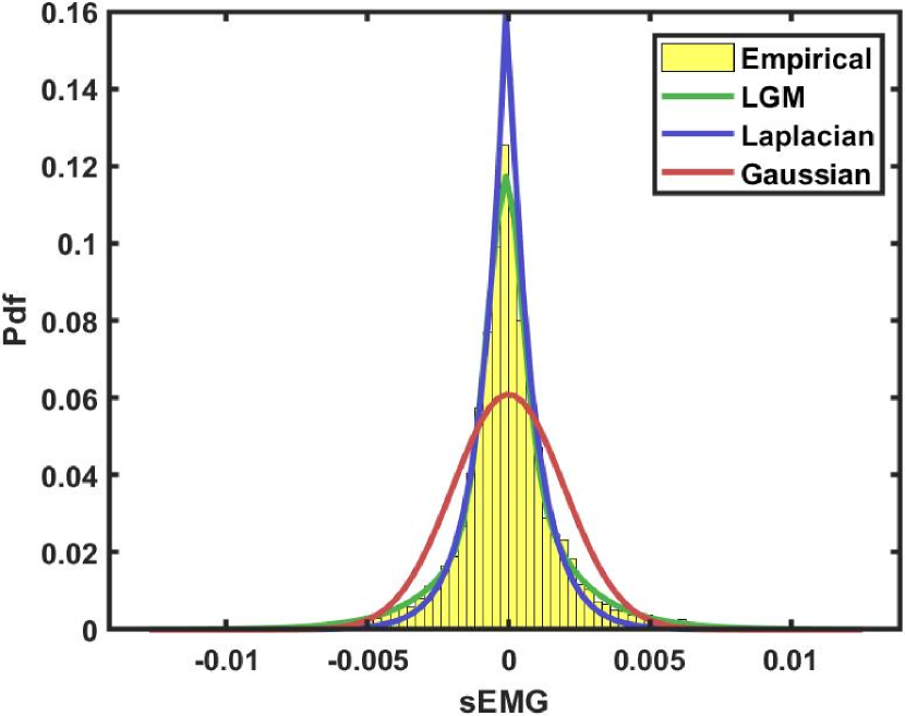
(a) Gestures

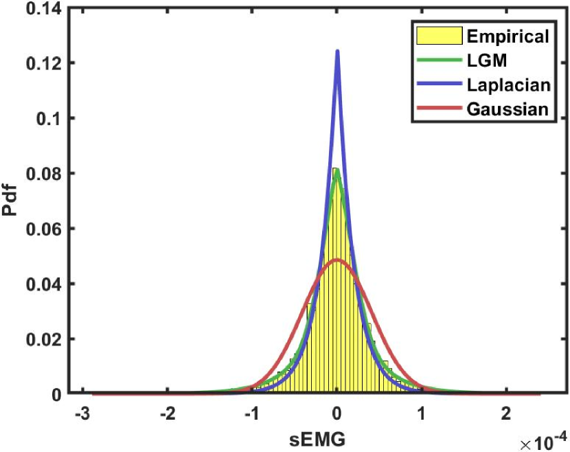
(b) Grasping

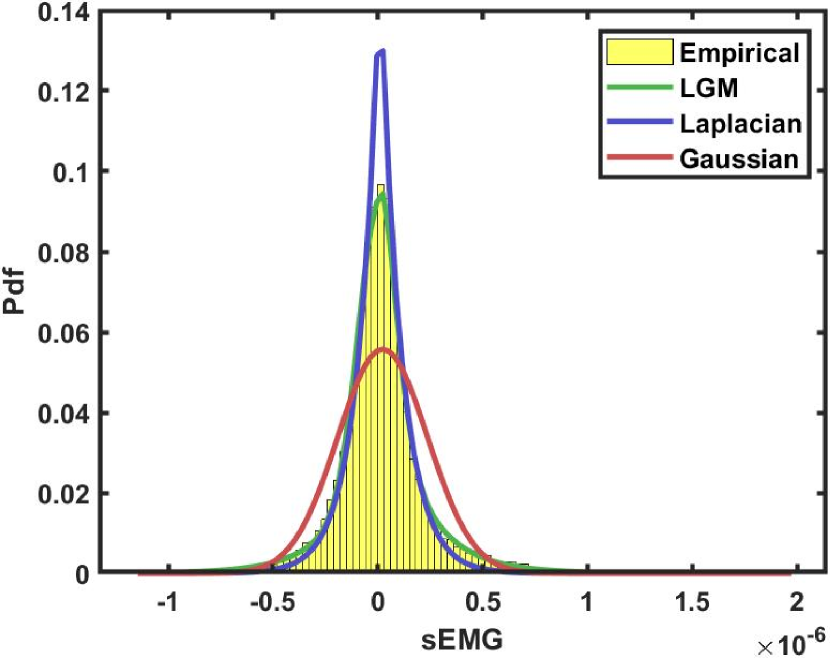
(c) Arm activity

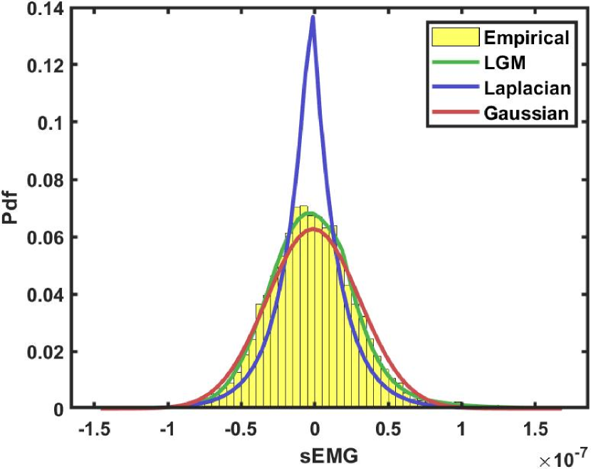
(d) Intense activity

Figure 1: Visual comparisons between mpdfs and estimated pdfs from models: LGM(green), Laplacian(blue) and Gaussian(red) for gestures, grasping, arm and intense activities for the subjects - 10, 3, 1 and 10 with corresponding activities - 7, 18, 3 and 1

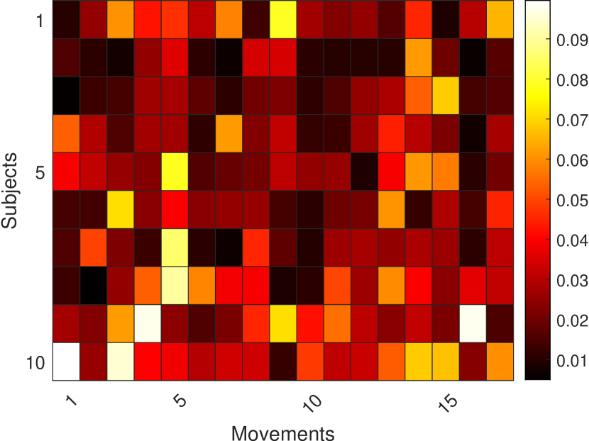
(a)

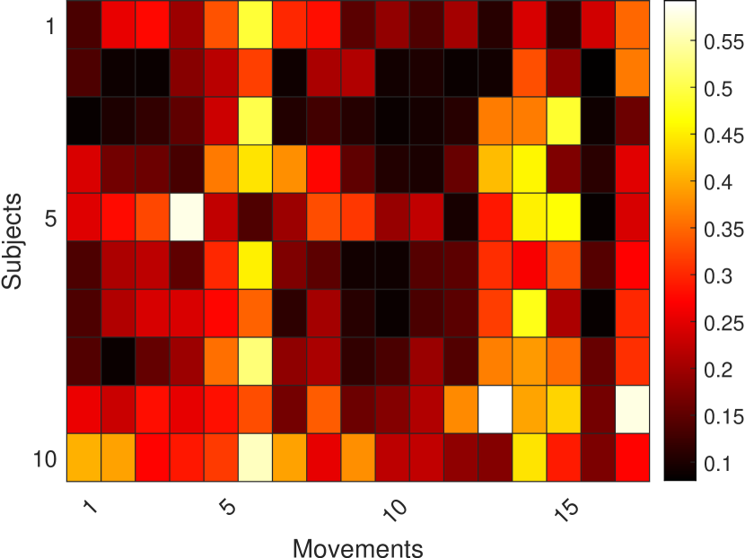
(b)

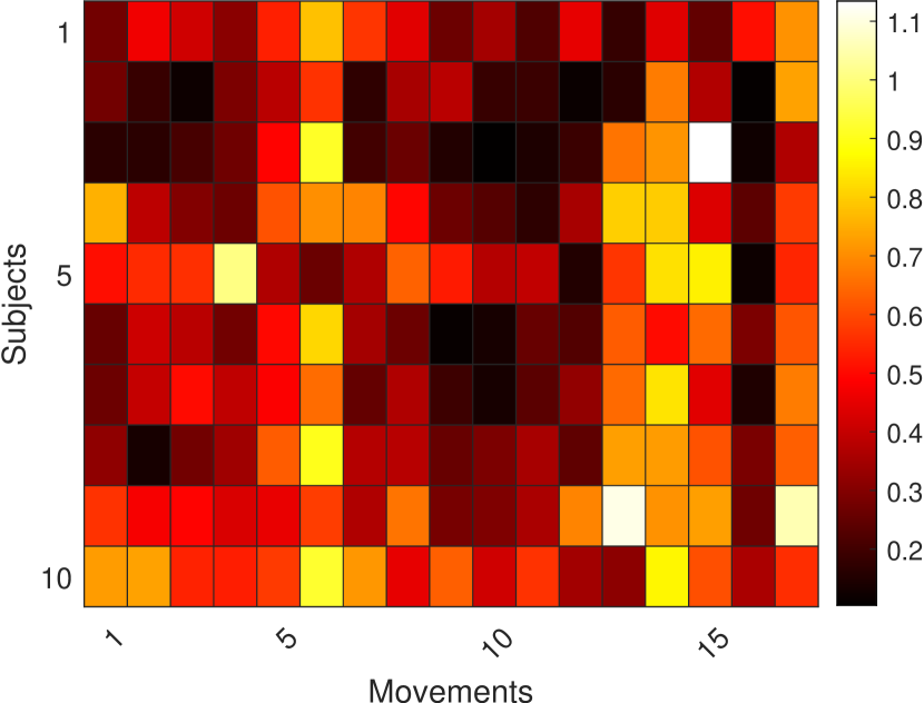
(c)

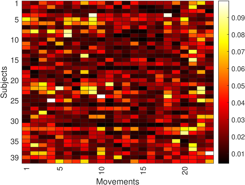
(d)

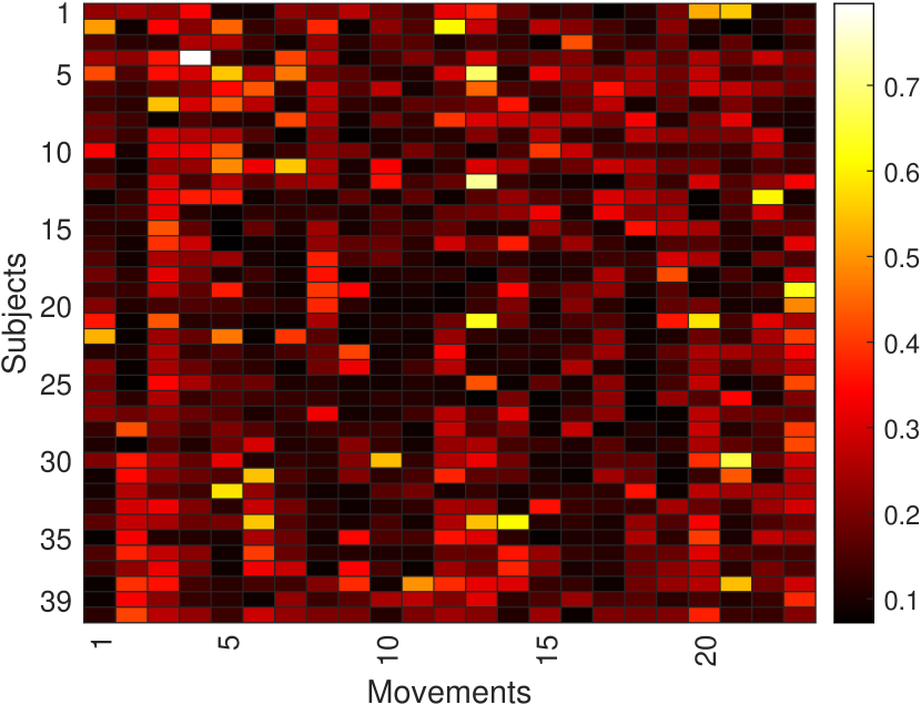
(e)

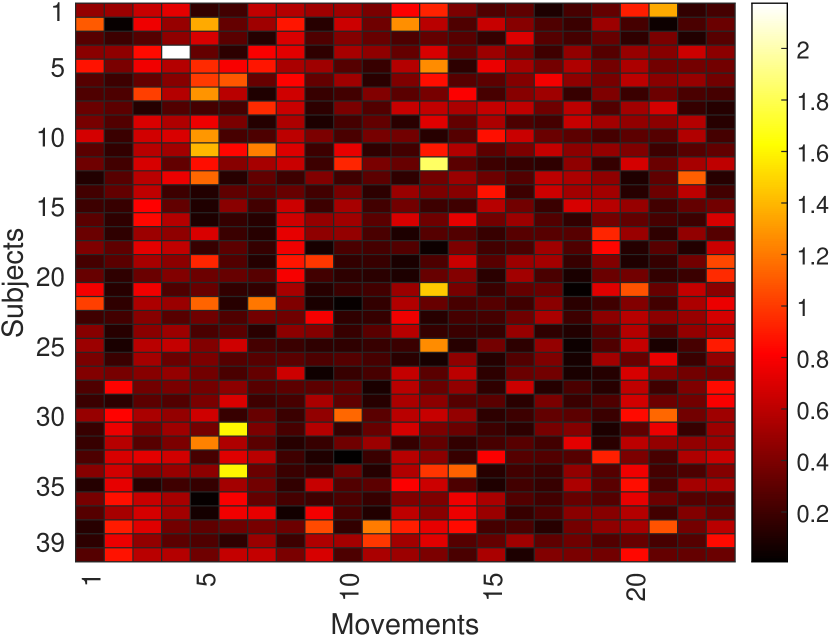
(f)

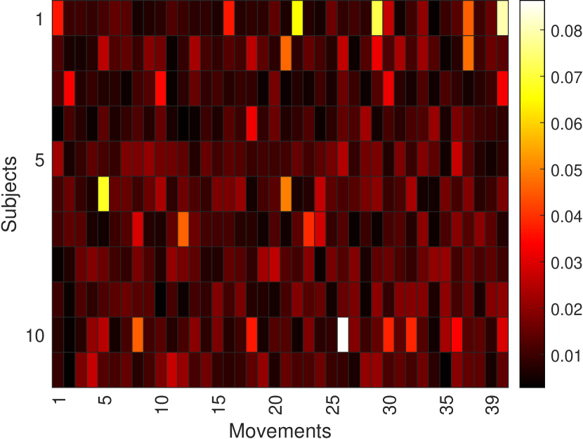
(g)

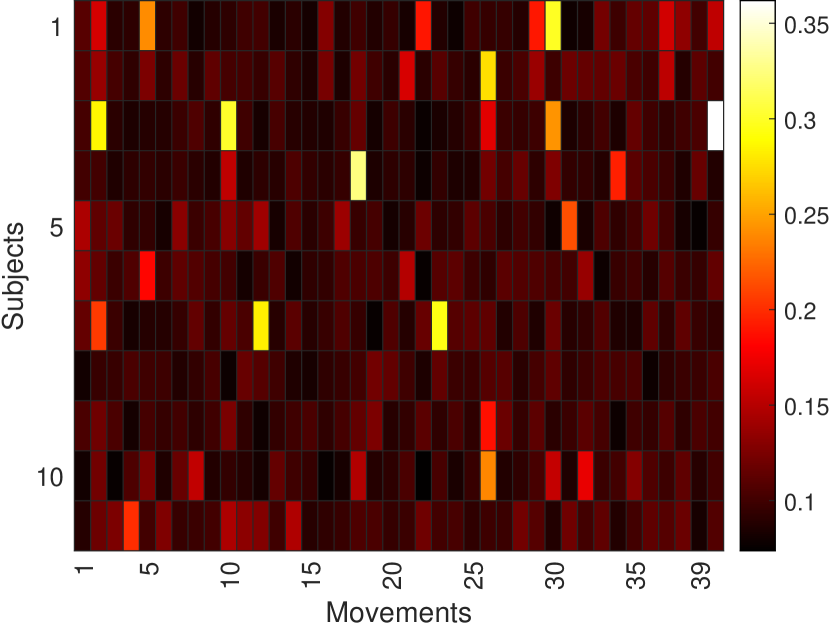
(h)

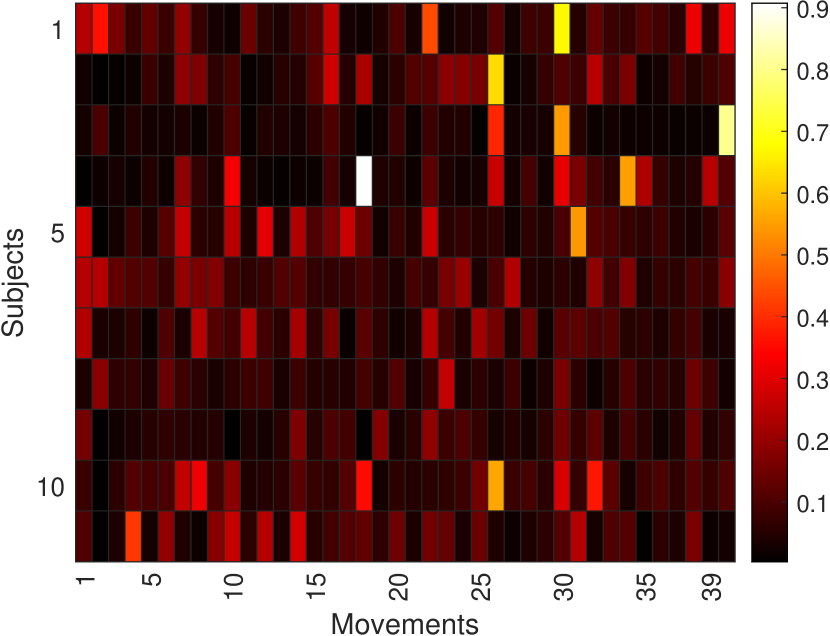
(i)

Figure 2: Heatmaps of KLD for the 3 models: (a) LGM, (b) Laplacian and (c) Gaussian corresponding to Ninapro-DB4, (d) LGM, (e) Laplacian and (f) Gaussian from Ninapro-DB2 and (g) LGM, (h) Laplacian and (i) Gaussian from Rami-khushaba-DB6

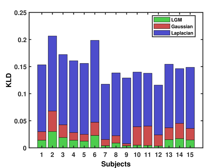
Figure 3: KLD values of LGM, Laplacian and Gaussian models for intense activity data

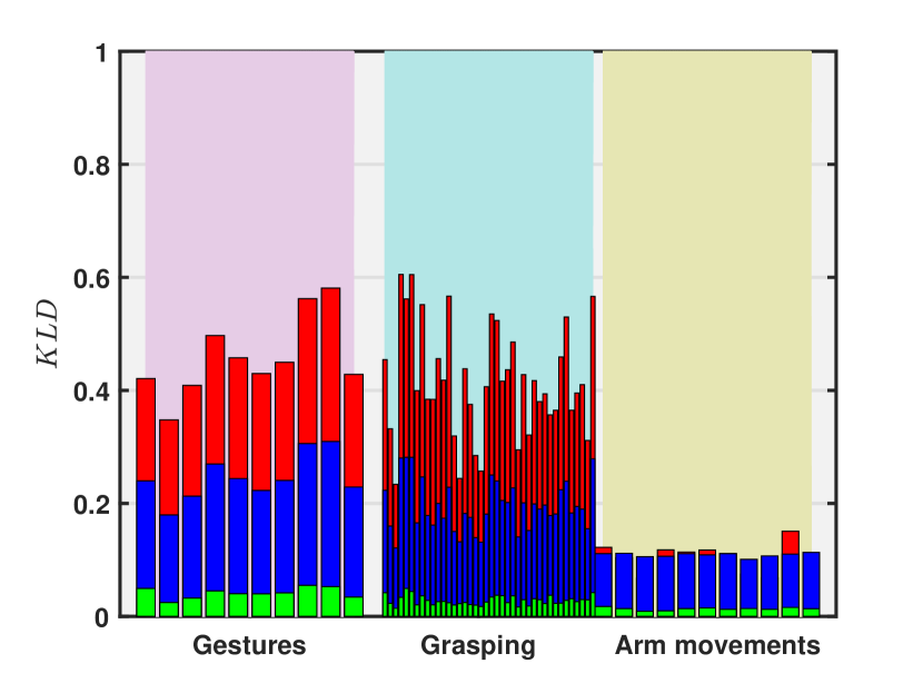
(a)

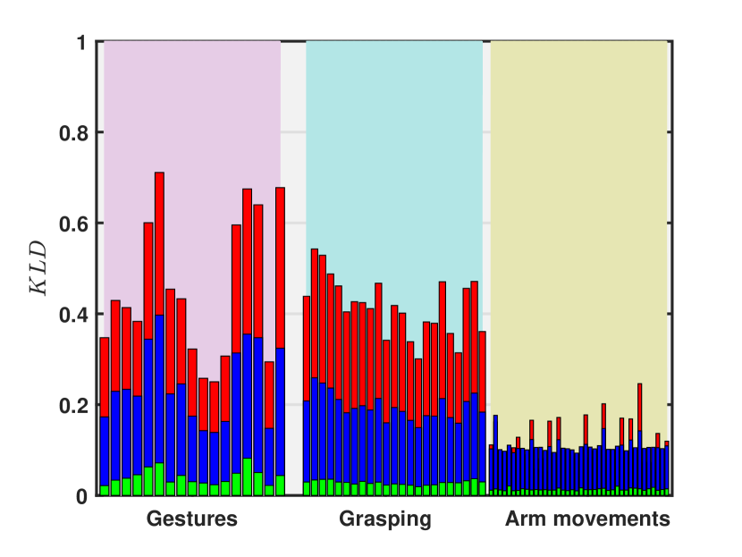
(b)

Figure 4: Average KLD for the 3 models (LGM-green, Laplacian-blue, Gaussian-red) for each of the trails (a) over the movements for different subjects (b) over the subjects for different movements

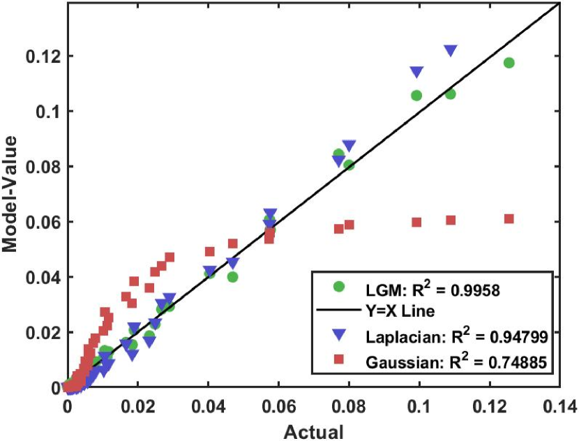
(a) Gestures

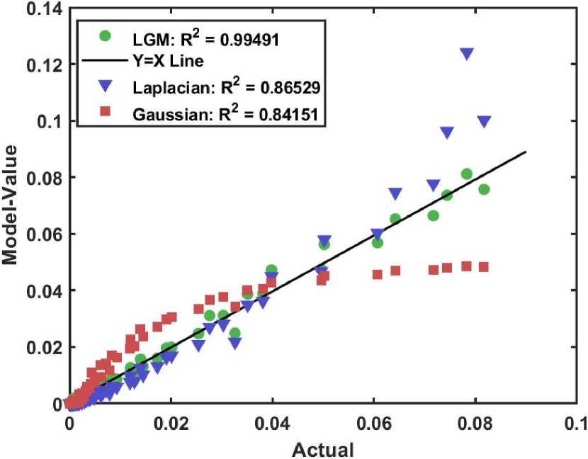
(b) Grasping

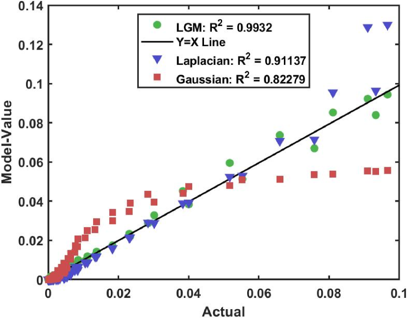
(c) Normal activity

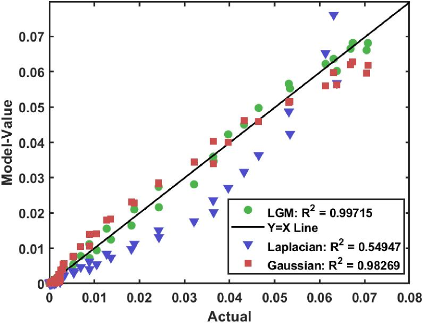
(d) Intense activity

Figure 5: Goodness of fit plots for the models LGM(green), Laplacian(blue) and Gaussian(red) for gestures, grasping, normal and Intense activities for the subjects-10, 3, 1 and 10 and with corresponding activities-7, 18, 3 and 1

A goodness of fit plot with R-squared[38]: The relationship between the sEMG data and the model-based values is analyzed using a goodness of fit plot. The nearer the data points are to the line of equality, greater the model fit. On other hand, the coefficient of determination (R-squared) is a measure of how much the variance in the observed dependent variable is explained by the independent variable. The closer the value to $1$ greater the correlation between the two variables.

Likelihood ratio test (LRT): The LRT is a statistical test used to compare two different models. In order to determine which model is statistically significant the likelihood values are evaluated for both the models. The LRT is defined as [39]

$$T=2(log(L_{p})-log(L_{e}))$$ (21)

where $L_{p}$ and $L_{e}$ are likelihoods of the LGM model and any existing model respectively.

III Data Description

Please note that all of the datasets analyzed in this study are available through public sources. Their short descriptions follow.

• Ninapro Datasets:
  In Ninapro DB2 (NPDB2) [40] and DB4 (NPDB4) [41] datasets, there are $3$ exercises collected from groups of $40$ and $10$ subjects respectively. The exercises-$1$ and $2$ are related to activities such as hand gestures and grasping. The exercise-$3$ corresponds to finger movements at various forces levels including the abduction and adduction of the thumb. In this work, the EMG signals corresponding to the exercise- 2 from both the DB2 and DB4 are analyzed They consist of 23 grasping and 17 gesture actions respectively. The sEMG signals in this dataset have $12$ channels corresponding to a set of twelve electrodes placed at strategic muscle locations on an arm [41]. In this dataset, a typical sEMG signal within a activity, has a duration of $8$s with a $3$s rest time and $5$s activity. Each trial is repeated six times.

• Rami-khushaba DB6 (RKDB6) [42]:
  This dataset consists of sEMG signals collected from 11 intact subjects (9 males and 2 females) when they were performing $8$ different movements through $5$ limb positions. The limb positions were chosen in such a way that each subject can mimic daily activities. Each activity has six repetitions. A sEMG signal array consists of seven channels corresponding to seven Delsys DE $2.x$ EMG sensors placed across the circumference of the forearm

• Intense Action Dataset (IAD) [43]:
  This dataset consists of sEMG signals acquired from $15$ healthy subjects when performing a single intense activity i.e., each subject is instructed to hold a 6kg dumbbell with the right hand for 120 seconds. These sEMG signals consist of $8$ channels corresponding to $8$ EMG electrodes and each activity is carried out only once. The basic characteristics of these benchmark datasets are provided in the table I.

IV Results and Analysis

For each of the mentioned datasets, the sEMG signals corresponding to each trial from each activity by each subject are analyzed using the three models. Specifically, the sEMG signal from the channel with the highest energy among multiple channels is examined using the models based on the following evaluation methods.

• a qualitative analysis based on visual inspection

• quantitative analyses:

  1. the KL divergence analysis

  2. the goodness of fit plots with R-squared and confidence interval for R-squared

  3. the likelihood ratio test

IV-A Visual Inspection

Fig. 1 illustrates the visual comparisons between the mpdf (yellow) and the fitted pdfs from the LGM (green), the Laplacian (blue) and the Gaussian (red) models. These pdfs correspond to EMG signals of different activities as listed in the following: Fig. 1(a): activity-$7$ i.e., pointing index finger by subject-$10$, Fig. 1(b): activity-$18$ i.e., the quadpod grasp by subject-$3$, Fig. 1(c): activity-$3$ i.e., a wrist supination by subject-$1$ and Fig. 1(d): activity-$1$ i.e., lifting a dumbbell by subject-$10$. Figs. 1(a), (b) and (c) correspond to pdfs of the sEMG signal corresponding to gestures, grasping and normal arm activities. From these it is evident that the overlap between the mpdf and the LGM model is high compared to standalone Laplacian and Gaussian models. Whereas Fig. 1(d) represents the pdfs of the sEMG signal corresponding to the intense activity, it is noticed that the overlap between the LGM model and the mpdf is similar to that of the standalone Gaussian model and the mpdf. In contrast, the overlap between the standalone Laplacian model and mpdf is lower.

IV-B Quantitative Analysis

IV-B1 KL-divergence

For each of the datasets under consideration, the KLD is evaluated between the LGM pdf and the mpdf. For comparison purposes, the KLD computation is also done for the Gaussian and the Laplacian pdfs against the mpdf. The corresponding results are illustrated in Figs. 2 to 4. Specifically, the heatmaps of KLD as a function of subjects and movements are shown in Fig. 2. Each cell in a heatmap corresponds to the KLD for a given model for a particular subject while performing one of the activities. Further, the KLD represented here is an average over the given trials of an activity. Figs. 2 (a)-(c) correspond to the KLD for the Ninapro-DB4, Figs. 2 (d)-(f) depict the KLD for the Ninapro-DB2 and Figs. 2 (g)-(i) represent the KLD for the Rami-khushaba-DB6. For each of the three datasets, it is noted that in these heatmaps, the LGM model has the lowest KLD. The lower and upper bounds of KLD for the heatmaps in Fig. 2 are shown in table II. The key observation is the highest KLD value from the LGM model is the lowest KLD value for both the Laplacian and the Gaussian models.

TABLE II: Lower and upper bounds of KLD for the proposed and the standalone models for different datasets

Datasets	LGM	Laplacian	Gaussian
NPDB4	[0.01 0.1]	[0.1 0.6]	[0.1 1.1]
NPDB2	[0.01 0.1]	[0.1 0.8]	[0.1 2.2]
RKDB6	[0.01 0.1]	[0.1 0.35]	[0.1 0.9]

The KLD values for different models in the case of the intense activity are shown in Fig. 3. Notably, for the intense activity dataset as well, the KLD value is the lowest for the LGM model closely followed by the Gaussian model and then the Laplacian model. The minimum and maximum KLD values corresponding to the three models are: the LGM {0.0033, 0.0301}, the Gaussian {0.0039, 0.0378} and the Laplacian {0.0920, 0.1513}.

Fig. 4(a) shows the KLD averaged over the movements as a function of the subjects. Fig. 4(b) shows the vice versa case. The KLD of the LGM, Laplacian and Gaussian models are represented in green, blue and red respectively. From Fig. 4(a) and (b), it is observed that for the activities such as the gestures, grasping and the arm movements the average KLD value over the movements and subjects is the lowest for the LGM model, when compared to the other models.

IV-B2 Goodness of fit plots

Fig. 5 illustrates the goodness of fit plots between the estimates from the three models versus the actual data. Specifically, the Figs. 5 (a) to (d) correspond to the results on data from the gestures, grasping, normal arm and the intense activities respectively. The LGM model, Laplacian and Gaussian models are represented by the data points in green, blue and red respectively. From Figs. 5 (a), (b) and (c), in the scatter plots, the model-values of the LGM model are found to be adjacent to the line of equality which means that the predicted values from this model are close to the actual values of the sEMG signal. Whereas in the case of intense activity shown in Fig. 5(d), the model values corresponding to both the LGM and the Gaussian models are similar and they are adjacent to the line of equality. From Fig. 5, for the gestures, grasping and normal arm activities, it can be concluded that the LGM model is better compared to other models. However, for the intense activity, both the LGM and the Gaussian fit the EMG data quite well. The average R-squared values are shown in the table III. For the first three categories of activities, based on these metrics, the LGM model is found to be superior. Additionally, for the intense activities, the LGM and the Gaussian are again similar. The 95 percent confidence intervals(CI) [44] [45] for R-squared corresponding to the plots in Fig. 5 are given in table IV.

TABLE III: R-Squared values for four datasets from model evaluations

Datasets	LGM	Laplacain	Gaussian
NPDB4	0.9958	0.94799	0.74885
NPDB2	0.99491	0.86529	0.84151
RKDB6	0.9932	0.91137	0.82279
IAD	0.99715	0.54947	0.98269

TABLE IV: Confidence interval of R-squared for LGM, Laplacian and Gaussian models

Datasets	LGM	Laplacain	Gaussian
NPDB4	[0.9946 0.9970]	[0.9439 0.9520]	[0.7413 0.7564]
NPDB2	[0.9937 0.9961]	[0.8598 0.8708]	[0.8357 0.8473]
RKDB6	[0.9918 0.9946]	[0.9067 0.9160]	[0.8167 0.8289]
IAD	[0.9960 0.9983]	[0.5402 0.5587]	[0.9800 0.9854]

IV-B3 Likelihood ratio test

The LRT given in (21) is carried out between the LGM model and the Laplacian model as shown below.

$$H_{0}:$$ The Laplacian model fits the data

$$H_{1}:$$ The LGM model fits the data

This test is carried out for $99\%$ confidence interval. It is noted that p-value is less than $0.01$, which means $H_{0}$ is rejected and $H_{1}$ is accepted. The test is repeated by replacing the Laplacian with the Gaussian model for $H_{0}$. In this test also the p-value is found to be less than $0.01$ and thus $H_{1}$ is accepted.

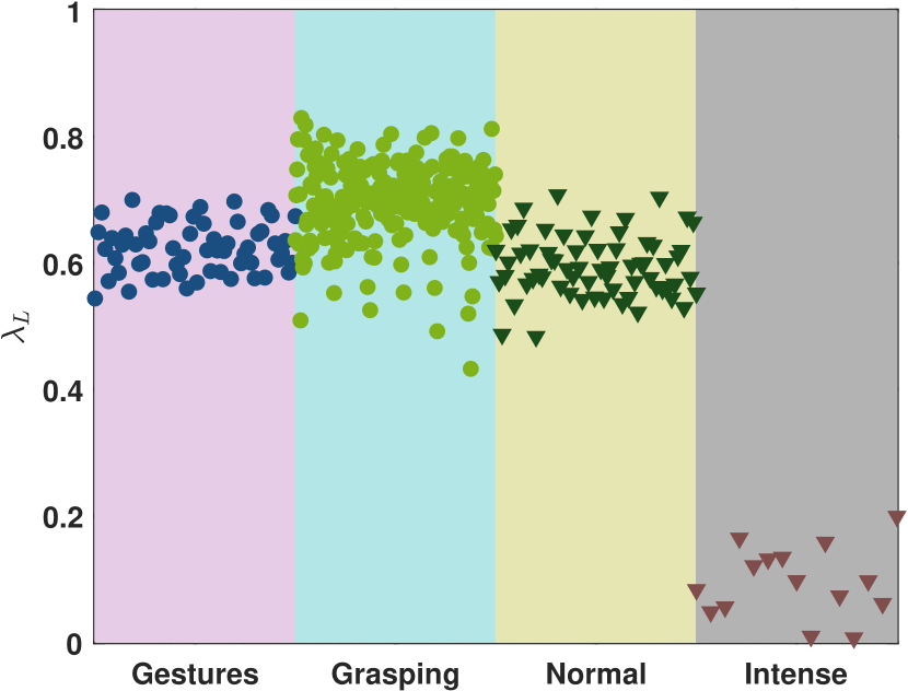
Figure 6: Laplacian coefficient for each trail versus subjects for gestures, grasping, normal arm movements and intense activity

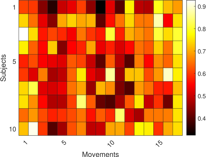
(a)

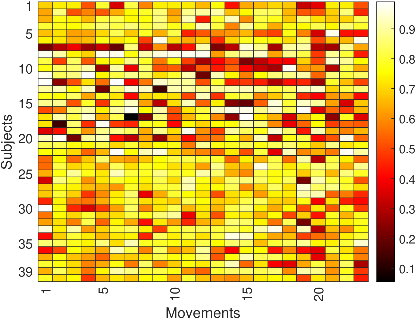
(b)

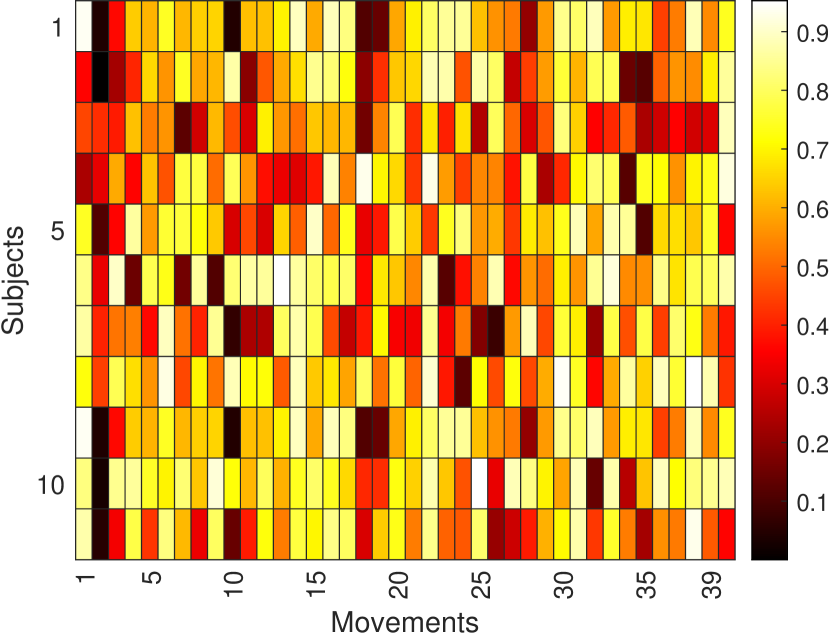
(c)

Figure 7: Laplacian weights of LGM model averaged over trials as a function of subjects and movements for (a) gestures, (b) grasping, and (C) arm activities

IV-C Mixing Weights

The mixing coefficients corresponding to the Laplacian component of the LGM model corresponding to different activities from various datasets are shown in Fig. 6. For the low and medium MCF levels such as the gestures, grasping and the normal activities, it is noticed that the Laplacian component has a stronger weighting in comparison with the Gaussian component. Whereas in case of intense activity i.e., at high MCF level the mixing weight corresponding to the Gaussian component is higher and the Laplacian component is lower. Thus from Fig. 6, it can be recognized that as the intensity of an activity, i.e., the amount of energy required for performing a certain action increases, the weight of the Laplacian component reduces. Fig. 7 shows Laplacian weights of the LGM model corresponding to the first three limb activities under consideration. The horizontal and vertical axes in the heatmaps correspond to the number of movements and subjects respectively. Each cell in a heatmap denotes the Laplacian weight in the LGM model for a particular subject and activity. It is noticed that for most of the cases the Laplacian weight $\lambda_{1}$ is dominating the Gaussian weight $\lambda_{2}$. In some circumstances, the Laplacian weights are lower than Gaussian weights. For example, in Fig. 7 (a) for the subject-$1$, activities-$4$ and $9$, in Fig. 7(b) for the subject-$18$, activity-$2$ and in Fig. 7 (c), the subject-$1$, activities-$2$ and $10$, the Gaussian weights are stronger.

V Discussion

From the results presented in section IV, for the EMG signals corresponding to the low and medium levels of muscle recruitment i.e., for activities such as the gestures, grasping and the normal arm movements, the LGM is found to be a more suitable model compared to the standalone models. This is verified in terms of 1) the visual inspection between a model pdf and the mpdf, 2) the lowest KLD, 3) the goodness of fit plots - the model values matching the true values, 4) the higher R-squared values and 5) the Likelihood ratio test accepting the alternate hypothesis. However, in the case of intense activities, both the LGM and the Gaussian model seem to perform quite similarly according to the four evaluation methods described above. Hence for high levels of muscle recruitment, the proposed LGM model behaves similar to a standalone Gaussian model. This result is further qualified by the following observation, in the LGM model, the mixing coefficient of the Laplacian component becomes very small in comparison to that of the Gaussian component.

In the analysis on mixing weights, it is observed that for the first three types of actions, both the Laplacian and Gaussian components have significant contributions to the model. However, for the intense activity, the Gaussian component is much stronger. Hence, from these findings it can be postulated that the weights of the LGM model can be related to MCF level and motor units that are activated during an activity. For example, for the first three activities, the Laplacian weight $\lambda_{1}$ is higher relating to lower MCF level and the lower number of activated motor units. However, in the case of intense activity the Gaussian weight $\lambda_{2}$ is higher connecting to a higher MCF level and a larger number of activated motor units. These findings are in agreement with the literature on pdfs reported in section I-B where it is noted that for the lower and medium MCF levels, the pdfs have a sharper peak at center, hinting a Laplacian structure, and at higher MCF levels, they have a clear Gaussian structure.

VI Conclusion

In this paper, a Laplacian Gaussian mixture model is proposed for sEMG signals from upper limbs. The proposed model is tested on several benchmark sEMG datasets and compared with the existing standalone models. The suitability of the model is validated using (1) qualitative analyses such as visual comparison with the empirical pdf (mpdf) where it is observed that the LGM model has the best agreement, (2) the KL divergence between the model pdf and the mpdf, again the KLD is lowest for the LGM model, (3) a goodness of fit plot, comparison of coefficient of determination (CFD) - $R^{2}$ and confidence intervals for $R^{2}$, here it is noted that $R^{2}$ in case of the LGM model is closest to unity and (4) the Likelihood ratio test (LRT) that also supported the LGM model. Finally, it is noted, for the low and medium muscle contraction force levels, the Laplacian weight has stronger weighting than the Gaussian. Whereas for the higher muscle contraction force levels the Laplacian weights are lower. In the future work, we will extend the proposed model to understand the correlations between the sEMG signals from various muscle locations.

References

- [1] W. Wang, A. D. Stefano, and R. Allen, “A simulation model of the surface EMG signal for analysis of muscle activity during the gait cycle,” Computers in biology and medicine, vol. 36, no. 6, pp. 601–618, 2006.
- [2] D. W. Stashuk, “Simulation of electromyographic signals,” Journal of Electromyography and Kinesiology, vol. 3, no. 3, pp. 157–173, 1993.
- [3] P. A. Cuddon, “Electrophysiology in neuromuscular disease,” Veterinary Clinics: Small Animal Practice, vol. 32, no. 1, pp. 31–62, 2002.
- [4] A. D. Vigotsky, I. Halperin, G. J. Lehman, G. S. Trajano, and T. M. Vieira, “Interpreting signal amplitudes in surface electromyography studies in sport and rehabilitation sciences,” Frontiers in physiology, vol. 8, p. 985, 2018.
- [5] C. J. De Luca, “The use of surface electromyography in biomechanics,” Journal of applied biomechanics, vol. 13, no. 2, pp. 135–163, 1997.
- [6] G. L. Soderberg and T. M. Cook, “Electromyography in biomechanics,” Physical Therapy, vol. 64, no. 12, pp. 1813–1820, 1984.
- [7] E. Hasanbelliu, “A multi-dimensional visualization tool for understanding the role of EMG signals in head movement anticipation,” in ACM SIGGRAPH 2004 Posters, 2004, p. 109.
- [8] R. Merletti, L. L. Conte, E. Avignone, and P. Guglielminotti, “Modeling of surface myoelectric signals. i. model implementation,” IEEE Transactions on Biomedical Engineering, vol. 46, no. 7, pp. 810–820, 1999.
- [9] J. Rodriguez-Falces, J. Navallas, and A. Malanda, “Emg modeling,” Computational Intelligence in Electromyography Analysis-A Perspective on Current Applications and Future Challenges, pp. 3–36, 2012.
- [10] M. Hayashibe and D. Guiraud, “Voluntary EMG-to-force estimation with a multi-scale physiological muscle model,” Biomedical engineering online, vol. 12, no. 1, pp. 1–18, 2013.
- [11] O. Paiss and G. F. Inbar, “Autoregressive modeling of surface EMG and its spectrum with application to fatigue,” IEEE Transactions on Biomedical Engineering, no. 10, pp. 761–770, 1987.
- [12] T. Kiryu, C. J. De Luca, and Y. Saitoh, “AR modeling of myoelectric interference signals during a ramp contraction,” IEEE Transactions on Biomedical Engineering, vol. 41, no. 11, pp. 1031–1038, 1994.
- [13] S. Shahid, J. Walker, G. M. Lyons, C. A. Byrne, and A. V. Nene, “Application of higher order statistics techniques to EMG signals to characterize the motor unit action potential,” IEEE Transactions on Biomedical Engineering, vol. 52, no. 7, pp. 1195–1209, 2005.
- [14] A. Furui, H. Hayashi, and T. Tsuji, “A scale mixture-based stochastic model of surface EMG signals with variable variances,” IEEE Transactions on Biomedical Engineering, vol. 66, no. 10, pp. 2780–2788, 2019.
- [15] Z. O. Khokhar, Z. G. Xiao, and C. Menon, “Surface EMG pattern recognition for real-time control of a wrist exoskeleton,” Biomedical engineering online, vol. 9, no. 1, pp. 1–17, 2010.
- [16] H. Huang, T. A. Kuiken, R. D. Lipschutz et al., “A strategy for identifying locomotion modes using surface electromyography,” IEEE Transactions on Biomedical Engineering, vol. 56, no. 1, pp. 65–73, 2008.
- [17] A. D. Chan and K. Englehart, “Continuous classification of myoelectric signals for powered prostheses using gaussian mixture models,” in Proceedings of the 25th Annual International Conference of the IEEE Engineering in Medicine and Biology Society (IEEE Cat. No. 03CH37439), vol. 3. IEEE, 2003, pp. 2841–2844.
- [18] A. Furui, T. Igaue, and T. Tsuji, “EMG pattern recognition via bayesian inference with scale mixture-based stochastic generative models,” Expert Systems with Applications, vol. 185, p. 115644, 2021.
- [19] P. S. Giacomini, “Electromyography and neuromuscular disorders: clinical electrophysiologic correlations,” McGill Journal of Medicine: MJM, vol. 9, no. 2, p. 173, 2006.
- [20] D. Xiong, D. Zhang, X. Zhao, and Y. Zhao, “Deep learning for EMG-based human-machine interaction: A review,” IEEE/CAA Journal of Automatica Sinica, vol. 8, no. 3, pp. 512–533, 2021.
- [21] W. Wei, Q. Dai, Y. Wong, Y. Hu, M. Kankanhalli, and W. Geng, “Surface-electromyography-based gesture recognition by multi-view deep learning,” IEEE Transactions on Biomedical Engineering, vol. 66, no. 10, pp. 2964–2973, 2019.
- [22] B. Hudgins, P. Parker, and R. N. Scott, “A new strategy for multifunction myoelectric control,” IEEE Transactions on Biomedical Engineering, vol. 40, no. 1, pp. 82–94, 1993.
- [23] H. Roesler, “Statistical analysis and evaluation of myoelectric signals for proportional control,” The Control of upper-extremity prostheses and orthoses, pp. 44–53, 1974.
- [24] H. Milner-Brown and R. Stein, “The relation between the surface electromyogram and muscular force.” The Journal of physiology, vol. 246, no. 3, pp. 549–569, 1975.
- [25] P. A. Parker, J. A. Stuller, and R. N. Scott, “Signal processing for the multistate myoelectric channel,” Proceedings of the IEEE, vol. 65, no. 5, pp. 662–674, 1977.
- [26] I. Hunter, R. Kearney, and L. Jones, “Estimation of the conduction velocity of muscle action potentials using phase and impulse response function techniques,” Medical and Biological Engineering and Computing, vol. 25, no. 2, pp. 121–126, 1987.
- [27] M. Bilodeau, M. Cincera, A. B. Arsenault, and D. Gravel, “Normality and stationarity of EMG signals of elbow flexor muscles during ramp and step isometric contractions,” Journal of Electromyography and Kinesiology, vol. 7, no. 2, pp. 87–96, 1997.
- [28] E. A. Clancy and N. Hogan, “Probability density of the surface electromyogram and its relation to amplitude detectors,” IEEE Transactions on Biomedical Engineering, vol. 46, no. 6, pp. 730–739, 1999.
- [29] P. Kaplanis, C. S. Pattichis, L. Hadjileontiadis, and S. M. Panas, “Bispectral analysis of surface EMG,” in 2000 10th Mediterranean Electrotechnical Conference. Information Technology and Electrotechnology for the Mediterranean Countries. Proceedings. MeleCon 2000 (Cat. No. 00CH37099), vol. 2. IEEE, 2000, pp. 770–773.
- [30] K. Nazarpour, A. Sharafat, and S. Firoozabadi, “Negentropy analysis of surface electromyogram signal,” in IEEE/SP 13th Workshop on Statistical Signal Processing, 2005. IEEE, 2005, pp. 974–977.
- [31] G. R. Naik and D. K. Kumar, “Evaluation of higher order statistics parameters for multi channel sEMG using different force levels,” in 2011 Annual International Conference of the IEEE Engineering in Medicine and Biology Society. IEEE, 2011, pp. 3869–3872.
- [32] G. R. Naik, D. K. Kumar, and S. P. Arjunan, “Kurtosis and negentropy investigation of myo electric signals during different MVCs,” in ISSNIP Biosignals and Biorobotics Conference 2011. IEEE, 2011, pp. 1–4.
- [33] K. Nazarpour, A. H. Al-Timemy, G. Bugmann, and A. Jackson, “A note on the probability distribution function of the surface electromyogram signal,” Brain research bulletin, vol. 90, pp. 88–91, 2013.
- [34] D. Kusuru, A. C. Turlapaty, and M. Thakur, “A laplacian-gaussian mixture model for surface EMG signals from upper limbs,” in 2021 43rd Annual International Conference of the IEEE Engineering in Medicine & Biology Society (EMBC). IEEE, 2021, pp. 681–685.
- [35] C. M. Bishop and N. M. Nasrabadi, Pattern recognition and machine learning. Springer, 2006, vol. 4, no. 4.
- [36] A. Spanos, Probability Theory and Statistical Inference: Empirical Modeling with Observational Data. Cambridge University Press, 2019.
- [37] S. Kullback, Information theory and statistics. Courier Corporation, 1997.
- [38] J. Cohen, P. Cohen, S. G. West, and L. S. Aiken, “Applied multiple regression,” Correlation Analysis for the Behavioral Sciences, vol. 2, 1983.
- [39] G. King, Unifying political methodology: The likelihood theory of statistical inference. University of Michigan Press, 1998.
- [40] M. Atzori, A. Gijsberts, C. Castellini, B. Caputo, A.-G. M. Hager, S. Elsig, G. Giatsidis, F. Bassetto, and H. Müller, “Electromyography data for non-invasive naturally-controlled robotic hand prostheses,” Scientific Data, vol. 1, no. 1, pp. 1–13, 2014.
- [41] S. Pizzolato, L. Tagliapietra, M. Cognolato, M. Reggiani, H. Müller, and M. Atzori, “Comparison of six electromyography acquisition setups on hand movement classification tasks,” PloS one, vol. 12, no. 10, p. e0186132, 2017.
- [42] R. N. Khushaba, M. Takruri, J. V. Miro, and S. Kodagoda, “Towards limb position invariant myoelectric pattern recognition using time-dependent spectral features,” Neural Networks, vol. 55, pp. 42–58, 2014.
- [43] A. Ebied, A. M. Awadallah, M. A. Abbass, and Y. El-Sharkawy, “Upper limb muscle fatigue analysis using multi-channel surface EMG,” in 2020 2nd Novel Intelligent and Leading Emerging Sciences Conference (NILES). IEEE, 2020, pp. 423–427.
- [44] J. D. Finn et al., “Correlations redux,” Psychological Bulletin, vol. 118, no. 1, pp. 155–164, 1995.
- [45] P. Cohen, S. G. West, and L. S. Aiken, Applied multiple regression/correlation analysis for the behavioral sciences. Psychology press, 2014.