LEAST PRODUCT RELATIVE ERROR

ESTIMATION FOR FUNCTIONAL

MULTIPLICATIVE MODEL AND

OPTIMAL SUBSAMPLING

Qian Yan, Hanyu Li

Chongqing University

Abstract: In this paper, we study the functional linear multiplicative model based on the least product relative error criterion. Under some regularization conditions, we establish the consistency and asymptotic normality of the estimator. Further, we investigate the optimal subsampling for this model with massive data. Both the consistency and the asymptotic distribution of the subsampling estimator are first derived. Then, we obtain the optimal subsampling probabilities based on the A-optimality criterion. Moreover, the useful alternative subsampling probabilities without computing the inverse of the Hessian matrix are also proposed, which are easier to implement in practise. Finally, numerical studies and real data analysis are done to evaluate the performance of the proposed approaches.

Key words and phrases: Asymptotic normality, functional multiplicative model, least product relative error, massive data, optimal subsampling

1 Introduction

In the era of big data, data can be collected and recorded on a dense sample of observations in time and space. These observations are of a functional nature and typically take the form of curves and images. Functional data analysis has been shown to perform wonderfully well with these datasets. Functional regression models with scalar response have been extensively studied and the most popular one is the functional linear model.

We consider a scalar-on-function linear multiplicative model

$$y=\exp\left(\int^{1}_{0}X(t)\beta(t)\mathrm{d}t\right)\epsilon,\$$ (1.1)

where the covariate $X(t)$ and slope $\beta(t)$ are smooth and square integrable functions defined on $[0,1]$, $y$ is the scalar response variable, and $\epsilon$ is the random error. Moreover, both $y$ and $\epsilon$ are strictly positive. By taking the logarithmic transformation, the model (1.1) becomes the regular functional linear model. However, in comparison, the multiplicative model is more useful and flexible to handle positive responses such as incomes, stock prices and survival times.

As we know, to estimate the slope, absolute errors are the most popular choices for designing loss functions, such as the least squares (LS) and the least absolute deviation (LAD). However, in practical applications, loss functions based on relative errors may be more effective and suitable. There are two types of relative errors, relative to the target value $y$ and relative to the prediction of $y$. Chen et al. (2010) summed the two relative errors and proposed the least absolute relative error (LARE) criterion for scalar linear multiplicative model. However, the LARE criterion is non-smooth, which makes calculating it a little complicated. Later, by multiplying the two relative errors, Chen et al. (2016) improved it and presented the least product relative error (LPRE) criterion. The LPRE criterion is infinitely differentiable and strictly convex, resulting in a simple and unique estimator. Moreover, they also proved that the LPRE estimation is more effective than the LARE, LAD, and LS estimations under some certain conditions. As a result, this criterion has also been widely used in other scalar multiplicative models (Chen and Liu (2021); Chen, Liu and Ma (2022); Ming, Liu and Yang (2022)).

For functional multiplicative models, to the best of our knowledge, there are only a few works and all of them focus on the LARE criterion. For example, Zhang, Zhang and Li (2016) extended the LARE criterion to the functional model for the first time. They developed the functional quadratic multiplicative model and derived the asymptotic properties of the estimator. Later, Zhang et al. (2019) and Fan, Zhang and Wu (2022) considered the variable selection for partially and locally sparse functional linear multiplicative models based on the LARE criterion, respectively. It seems that there is no study on the LPRE criterion conducted for functional data. To fill the gap, we propose the LPRE criterion for the functional linear multiplicative model, and derive the consistency and asymptotic normality of the estimator.

Considering that traditional techniques are no longer usable for massive data due to the limitation of computational resources, several researchers have devoted to developing efficient or optimal subsampling strategies for statistical models with massive data. For example, for linear model, Ma, Mahoney and Yu (2015) studied the biases and variance of the algorithmic leveraging estimator. Ma et al. (2020) further provided the asymptotic distributions of the RandNLA subsampling estimators. For logistic regression, Wang, Zhu and Ma (2018) proposed an optimal subsampling method based on some optimality criteria (Atkinson, Donev and Tobias (2007)). Subsequently, Wang (2019) proposed a more efficient estimation method and Poisson subsampling to improve the estimation and computation efficiency. Later, Yao and Wang (2019), Yu, Wang and Ai (2020) and Ai et al. (2021b) extended the optimal subsampling method to softmax regression, quasi-likelihood and generalized linear models, respectively. Furthermore, considering the effect of heavy-tailed errors or outliers in responses, some scholars have investigated more robust models. For example, Wang and Ma (2021), Ai et al. (2021a), Fan, Liu and Zhu (2021), and Shao, Song and Zhou (2022) employed the optimal subsampling method in ordinary quantile regression, and Shao and Wang (2021) and Yuan et al. (2022) developed the subsampling for composite quantile regression. Very recently, Ren, Zhao and Wang (2022) considered the optimal subsampling strategy based on the LARE criterion in linear multiplicative model. They derived the asymptotic distribution of the subsampling estimator and proved that LARE outperforms LS and LAD under the optimal subsampling strategy. Wang and Zhang (2022) further extended the optimal subsampling to linear multiplicative model based on the LPRE criterion.

For functional regression models, now only little work has been done in the area of subsampling (Liu, You and Cao (2021); He and Yan (2022); Yan, Li and Niu (2022)). Specifically, He and Yan (2022) proposed a functional principal subspace sampling probability for functional linear regression with scalar response, which eliminates the impact of eigenvalue inside the functional principal subspace and properly weights the residuals. Liu, You and Cao (2021) and Yan, Li and Niu (2022) extended the optimal subsampling method to functional generalized linear models and functional quantile regression with scalar response, respectively.

Inspired by the above works, we further study the optimal subsampling for functional linear multiplicative model based on the LPRE criterion, and first establish the consistency and asymptotic normality of the subsampling estimator. Then, the optimal subsampling probabilities are obtained by minimizing the asymptotic integrated mean squared error (IMSE) under the A-optimality criterion. In addition, a useful alternative minimization criterion is also proposed to further reduce the computational cost.

The rest of this paper is organized as follows. Section 2 introduces the functional linear multiplicative model based on the LPRE criterion and investigates the asymptotic properties of the estimator. In Section 3, we present the asymptotic properties of the subsampling estimator and the optimal subsampling probabilities. The modified version of these probabilities is also considered in this section. Section 4 and Section 5 illustrate our methodology through numerical simulations and real data, respectively.

2 LPRE estimation

2.1 Estimation

Suppose that $\{(x_{i}(t),y_{i}),i=1,2,\ldots,n\}$ are samples from the model (1.1) with the independent and identical distribution. The functional LPRE estimator for the model (1.1), says $\hat{\beta}(t)$, is established by

$$\arg\inf\limits_{\beta}\sum_{i=1}^{n}\left\{\left\lvert\frac{y_{i}-\exp\left(\int^{1}_{0}x_{i}(t)\beta(t)\mathrm{d}t\right)}{y_{i}}\right\rvert\ \times\ \left\lvert\frac{y_{i}-\exp\left(\int^{1}_{0}x_{i}(t)\beta(t)\mathrm{d}t\right)}{\exp\left(\int^{1}_{0}x_{i}(t)\beta(t)\mathrm{d}t\right)}\right|\right\},$$

which is equivalent to

$$\arg\inf\limits_{\beta}\sum_{i=1}^{n}\left\{y_{i}\exp\left(-\int^{1}_{0}x_{i}(t)\beta(t)\mathrm{d}t\right)+y_{i}^{-1}\exp\left(\int^{1}_{0}x_{i}(t)\beta(t)\mathrm{d}t\right)-2\right\}.$$

We aim to estimate the slope function $\beta(t)$ via a penalized spline method. Define $K$ equispaced interior knots as $0=t_{0}<t_{1}<\ldots<t_{K}<t_{K+1}=1$. Let $\boldsymbol{B}(t)=(B_{1}(t),B_{2}(t),\dots,B_{K+p+1}(t))^{T}$ be the set of the normalized B-spline basis functions of degree $p$ on each sub-interval $[t_{j},t_{j+1}],j=0,1,\ldots,K$ and $p-1$ times continuously differentiable on $[0,1]$. The details of the B-spline functions can be found in de Boor (2001). Our functional LPRE estimator $\hat{\beta}(t)$ of $\beta(t)$ is thus defined as

$$\hat{\beta}(t)=\sum_{j=1}^{K+p+1}\hat{\boldsymbol{\theta}}_{j}B_{j}(t)=\boldsymbol{B}^{T}(t)\hat{\boldsymbol{\theta}}_{full},$$

where $\hat{\boldsymbol{\theta}}_{full}$ minimizes the penalized functional LPRE loss function

$$L(\boldsymbol{\theta};\lambda,K)$$

$$= \sum_{i=1}^{n}\left\{y_{i}\exp\left(-\int^{1}_{0}x_{i}(t)\boldsymbol{B}^{T}(t)\boldsymbol{\theta}\mathrm{d}t\right)+y_{i}^{-1}\exp\left(\int^{1}_{0}x_{i}(t)\boldsymbol{B}^{T}(t)\boldsymbol{\theta}\mathrm{d}t\right)-2\right\}$$

$$+\frac{\lambda}{2}\int^{1}_{0}\left\{\left(\boldsymbol{B}^{(q)}(t)\right)^{T}\boldsymbol{\theta}\right\}^{2}\mathrm{d}t,$$ (2.2)

where $\lambda>0$ is the smoothing parameter, and $\boldsymbol{B}^{(q)}(t)$ is the square integrated $q$-th order derivative of all the B-splines functions for some integer $q\leq p$. For convenience, we let $\boldsymbol{B}_{i}=\int_{0}^{1}x_{i}(t)\boldsymbol{B}(t)\mathrm{d}t$ and $\boldsymbol{D}_{q}=\int_{0}^{1}\boldsymbol{B}^{(q)}(t)\{\boldsymbol{B}^{(q)}(t)\}^{T}\mathrm{d}t$, the loss function (2.1) thus can be rewritten as

$$L(\boldsymbol{\theta};\lambda,K)=\sum_{i=1}^{n}\left\{\omega_{i}(\boldsymbol{\theta})+\omega_{i}(\boldsymbol{\theta})^{-1}-2\right\}+\frac{\lambda}{2}\boldsymbol{\theta}^{T}\boldsymbol{D}_{q}\boldsymbol{\theta},$$ (2.3)

where $\omega_{i}(\boldsymbol{\theta})=y_{i}\exp\left(-\boldsymbol{B}^{T}_{i}\boldsymbol{\theta}\right)$. Of note, the model (2.3) is infinitely differentiable and strictly convex. The Newton-Raphson method will be used since there is no general closed-form solution to the functional LPRE estimator. That is, the estimator $\hat{\boldsymbol{\theta}}_{full}$ can be obtained by iteratively applying the following formula until $\hat{\boldsymbol{\theta}}_{t+1}$ converges.

$$\hat{\boldsymbol{\theta}}_{t+1}= \hat{\boldsymbol{\theta}}_{t}-\left\{\sum_{i=1}^{n}\left(\omega_{i}(\hat{\boldsymbol{\theta}}_{t})+\omega_{i}(\hat{\boldsymbol{\theta}}_{t})^{-1}\right)\boldsymbol{B}_{i}\boldsymbol{B}^{T}_{i}+\lambda\boldsymbol{D}_{q}\right\}^{-1}$$

$$\times\left\{\sum_{i=1}^{n}\left(-\omega_{i}(\hat{\boldsymbol{\theta}}_{t})+\omega_{i}(\hat{\boldsymbol{\theta}}_{t})^{-1}\right)\boldsymbol{B}_{i}+\lambda\boldsymbol{D}_{q}\hat{\boldsymbol{\theta}}_{t}\right\}.$$

Note that the computational complexity for calculating $\hat{\boldsymbol{\theta}}_{full}$ is about $O(\zeta n(K+p+1)^{2})$, where $\zeta$ is the number of iterations until convergence. As we can see, the computational cost is expensive when the full data size $n$ is very large. To deal with this issue, we will propose a subsampling algorithm to reduce computational cost in Section 3.

2.2 Theoretical properties of $\hat{\beta}(t)$

We will show the consistency and asymptotic normality of $\hat{\beta}(t)$. For simplicity, the following notations are given firstly. For the function $f(t)$ belonging to Banach space, $\|f\|_{m}=(\int_{0}^{1}\lvert f(t)\rvert^{m}\mathrm{d}t)^{1/m}$ for $0<m<\infty$. For the matrix $\boldsymbol{A}=(a_{ij})$, $\|\boldsymbol{A}\|_{\infty}=\max_{ij}{\lvert a_{ij}\rvert}$. In addition, define $\boldsymbol{H}=\mathrm{E}\{\boldsymbol{B}\boldsymbol{B}^{T}(\epsilon+\epsilon^{-1})\}+\lambda/n\boldsymbol{D}_{q}$, $\boldsymbol{G}=\mathrm{E}\{\boldsymbol{B}\boldsymbol{B}^{T}(\epsilon-\epsilon^{-1})^{2}\}$, and

$$\hat{\boldsymbol{G}}=\frac{1}{n}\sum_{i=1}^{n}\left\{-\omega_{i}(\hat{\boldsymbol{\theta}}_{full})+\omega_{i}(\hat{\boldsymbol{\theta}}_{full})^{-1}\right\}^{2}\boldsymbol{B}_{i}\boldsymbol{B}^{T}_{i},$$

$$\hat{\boldsymbol{H}}=\frac{1}{n}\sum_{i=1}^{n}\left\{\omega_{i}(\hat{\boldsymbol{\theta}}_{full})+\omega_{i}(\hat{\boldsymbol{\theta}}_{full})^{-1}\right\}\boldsymbol{B}_{i}\boldsymbol{B}^{T}_{i}+\lambda/n\boldsymbol{D}_{q}.$$ (2.4)

Furthermore, we assume the following regularization conditions hold.

1. For the functional covariate $X(t)$, assume that $\mathrm{E}(\|X\|_{8}^{8})<\infty$.

2. Assume the unknown functional coefficient $\beta(t)$ is sufficiently smooth. That is, $\beta(t)$ has a $d^{\prime}$-th derivative $\beta^{(d^{\prime})}(t)$ such that

   $$\mid\beta^{(d^{\prime})}(t)-\beta^{(d^{\prime})}(s)\mid\leq C_{2}\mid t-s\mid^{v},\quad t,s\in[0,1],$$

   where the constant $C_{2}>0$ and $v\in[0,1]$. In what follows, we set $d=d^{\prime}+v\geq p+1$.

3. $\mathrm{E}\{(\epsilon-\epsilon^{-1})\mid X\}=0$.

4. $\mathrm{E}\{(\epsilon+\epsilon^{-1})^{6}\mid X\}<\infty$.

5. Assume the smoothing parameter $\lambda$ satisfies $\lambda=o(n^{1/2}K^{1/2-2q})$ with $q\leq p$.

6. Assume the number of knots $K=o(n^{1/2})$ and $K/n^{1/(2d+1)}\rightarrow\infty$ as $n\rightarrow\infty$.

Remark 1.

Assumptions (H.1) and (H.2) are quite usual in the functional setting (see e.g., Cardot, Ferraty and Sarda (2003); Claeskens, Krivobokova and Opsomer (2009)). Assumption (H.3) is an identifiability condition for the LPRE estimation of $\beta(t)$. Assumptions (H.3) and (H.4) ensure the consistency and asymptotic normality of the LPRE estimator. Assumptions (H.5) and (H.6) are mainly used to obtain the asymptotic unbiasedness of the LPRE estimator.

Now, we present the consistency and asymptotic normality of $\hat{\beta}(t)$.

Theorem 1.

Under Assumptions (H.1)–(H.6), for $t\in[0,1]$, as $n\rightarrow\infty$, we have

1. (Consistency) There exists a LPRE estimator $\hat{\beta}(t)$ such that

   $$\|\hat{\beta}-\beta\|_{2}=O_{P}(n^{-1/2}K^{1/2});$$

2. (Asymptotic normality)

   $$\{\boldsymbol{B}(t)^{T}\boldsymbol{V}_{full}\boldsymbol{B}(t)\}^{-1/2}\sqrt{n/K}(\hat{\beta}(t)-\beta(t))\to N(0,1)$$

   in distribution, where $\boldsymbol{V}_{full}=K^{-1}\boldsymbol{H}^{-1}\boldsymbol{G}\boldsymbol{H}^{-1}$, which is consistently estimated by $K^{-1}\hat{\boldsymbol{H}}^{-1}\hat{\boldsymbol{G}}\hat{\boldsymbol{H}}^{-1}$ defined in (2.2).

3 Optimal subsampling

3.1 Subsampling estimator and its theoretical properties

We first introduce a general random subsampling algorithm for the functional linear multiplicative model, in which the subsamples are taken at random with replacement based on some sampling distributions.

1. Sampling. Given a larger $K$, we generate $\boldsymbol{B}_{i}=\int_{0}^{1}x_{i}(t)\boldsymbol{B}(t)\mathrm{d}t$ and the new data is $\left\{(\boldsymbol{B}_{i},y_{i}),i=1,2,\ldots,n\right\}$. Assign the subsampling probabilities $\{\pi_{i}\}_{i=1}^{n}$ to all data points and draw a random subsample of size $r(\ll n)$ with replacement based on $\{\pi_{i}\}_{i=1}^{n}$ from the new data. Denote the subsample as $\{(\boldsymbol{B}_{i},y_{i},R_{i}),i=1,2,\ldots,n\}$, where $R_{i}$ denotes the total number of times that the $i$-th data point is selected from the full data and $\sum_{i=1}^{n}R_{i}=r$.

2. Estimation. Given $\lambda$, minimize the following loss function to get the estimate $\tilde{\boldsymbol{\theta}}$ based on the subsample,

   $$L^{\ast}(\boldsymbol{\theta};\lambda,K)=\frac{1}{r}\sum_{i=1}^{n}\frac{R_{i}}{\pi_{i}}\left(w_{i}(\tilde{\boldsymbol{\theta}}_{t})+w_{i}(\tilde{\boldsymbol{\theta}}_{t})^{-1}-2\right)+\frac{\lambda}{2}\boldsymbol{\theta}^{T}\boldsymbol{D}_{q}\boldsymbol{\theta}.$$ (3.5)

   Due to the convexity of $L^{\ast}(\boldsymbol{\theta};\lambda,K)$, the Newton-Raphson method is adopted until $\tilde{\boldsymbol{\theta}}_{t+1}$ and $\tilde{\boldsymbol{\theta}}_{t}$ are close enough,

   $$\tilde{\boldsymbol{\theta}}_{t+1}= \tilde{\boldsymbol{\theta}}_{t}-\left\{\sum_{i=1}^{n}\frac{R_{i}}{\pi_{i}}\left(\omega_{i}(\tilde{\boldsymbol{\theta}}_{t})+\omega_{i}(\tilde{\boldsymbol{\theta}}_{t})^{-1}\right)\boldsymbol{B}_{i}\boldsymbol{B}^{T}_{i}+\lambda D_{q}\right\}^{-1}$$

   $$\times\left\{\sum_{i=1}^{n}\frac{R_{i}}{\pi_{i}}\left(-\omega_{i}(\tilde{\boldsymbol{\theta}}_{t})+\omega_{i}(\tilde{\boldsymbol{\theta}}_{t})^{-1}\right)\boldsymbol{B}_{i}+\lambda D_{q}\tilde{\boldsymbol{\theta}}_{t}\right\}.$$ (3.6)

   Finally, we can get the subsample estimator $\tilde{\beta}(t)=\boldsymbol{B}^{T}(t)\tilde{\boldsymbol{\theta}}$.

The loss function (3.5) is guaranteed to be unbiased in cases when we use an inverse probability weighted technique since the subsampling probabilities $\pi_{i}$ may depend on the full data $\mathcal{F}_{n}=\{(x_{i}(t),y_{i}),i=1,2,\dots,n,t\in[0,1]\}$. Below we establish the consistency and asymptotic normality of $\tilde{\beta}(t)$ towards $\hat{\beta}(t)$. An extra condition is needed.

1. Assume that $\max_{1\leq i\leq n}r(n\pi_{i})^{-1}=O_{P}(1)$ and $r=o(K^{2})$.

Remark 2.

Assumption (H.7) is often used in inverse probability weighted algorithms to restrict the weights such that the loss function is not excessively inflated by data points with extremely small subsampling probabilities (Ai et al. (2021b); Liu, You and Cao (2021); Yan, Li and Niu (2022)).

Theorem 2.

Under Assumptions (H.1)–(H.7), for $t\in[0,1]$, as $r,n\rightarrow\infty$, conditionally on $\mathcal{F}_{n}$ in probability, we have

1. (Consistency) There exists a subsampling estimator $\tilde{\beta}(t)$ such that

   $$\|\tilde{\beta}-\hat{\beta}\|_{2}=O_{P\mid\mathcal{F}_{n}}(r^{-1/2}K^{1/2});$$

2. (Asymptotic normality)

   $$\left\{\boldsymbol{B}(t)^{T}\boldsymbol{V}\boldsymbol{B}(t)\right\}^{-1/2}\sqrt{r/K}(\tilde{\beta}(t)-\hat{\beta}(t))\rightarrow N(0,1)$$

   in distribution, where

   $$\boldsymbol{V}=\frac{1}{K}\hat{\boldsymbol{H}}^{-1}\boldsymbol{V}_{\pi}\hat{\boldsymbol{H}}^{-1},$$

   $$\boldsymbol{V}_{\pi}=\frac{1}{n^{2}}\sum_{i=1}^{n}\frac{1}{\pi_{i}}\left\{-\omega_{i}(\hat{\boldsymbol{\theta}}_{full})+\omega_{i}(\hat{\boldsymbol{\theta}}_{full})^{-1}\right\}^{2}\boldsymbol{B}_{i}\boldsymbol{B}^{T}_{i}.$$ (3.7)

3.2 Optimal subsampling probabilities

To better approximate $\hat{\beta}(t)$, it is important to choose the proper subsampling probabilities. A commonly used criterion is to minimize the asymptotic IMSE of $\tilde{\beta}(t)$. By Theorem 2, we have the asymptotic IMSE of $\tilde{\beta}(t)$ as follows

$$\mathrm{IMSE}(\tilde{\beta}(t)-\hat{\beta}(t))=\frac{K}{r}\int_{0}^{1}\boldsymbol{B}^{T}(t)\boldsymbol{V}\boldsymbol{B}(t)\mathrm{d}t.$$ (3.8)

Note that $\boldsymbol{V}$ defined in ((2):) is the asymptotic variance-covariance matrix of $\sqrt{r/K}(\tilde{\boldsymbol{\theta}}-\hat{\boldsymbol{\theta}}_{full})$ and the integral inequality $\int_{0}^{1}\boldsymbol{B}^{T}(t)\boldsymbol{V}\boldsymbol{B}(t)\mathrm{d}t\leq\int_{0}^{1}\boldsymbol{B}^{T}(t)\boldsymbol{V^{\prime}}\boldsymbol{B}(t)\mathrm{d}t$ holds if and only if $\boldsymbol{V}\leq\boldsymbol{V^{\prime}}$ holds in the Löwner-ordering sense. Thus, we focus on minimizing the asymptotic MSE of $\tilde{\boldsymbol{\theta}}$ and choose the subsampling probabilities such that $\mathrm{tr}(\boldsymbol{V})$ is minimized. This is called the A-optimality criterion in optimal experimental designs; see e.g., Atkinson, Donev and Tobias (2007). Using this criterion, we are able to derive the optimal subsampling probabilities provided in the following theorem.

Theorem 3 (A-optimality).

If the subsampling probabilities $\pi_{i},i=1,2,\dots,n,$ are chosen as

$$\pi_{i}^{FAopt}=\frac{\lvert-y_{i}\exp(-\boldsymbol{B}_{i}^{T}\hat{\boldsymbol{\theta}}_{full})+y_{i}^{-1}\exp(\boldsymbol{B}_{i}^{T}\hat{\boldsymbol{\theta}}_{full})\rvert\|\hat{\boldsymbol{H}}^{-1}\boldsymbol{B}_{i}\|_{2}}{\sum_{i=1}^{n}\lvert-y_{i}\exp(-\boldsymbol{B}_{i}^{T}\hat{\boldsymbol{\theta}}_{full})+y_{i}^{-1}\exp(\boldsymbol{B}_{i}^{T}\hat{\boldsymbol{\theta}}_{full})\rvert\|\hat{\boldsymbol{H}}^{-1}\boldsymbol{B}_{i}\|_{2}},$$ (3.9)

then the total asymptotic MSE of $\sqrt{r/K}(\tilde{\boldsymbol{\theta}}-\hat{\boldsymbol{\theta}}_{full})$, $\mathrm{tr}(\boldsymbol{V})$, attains its minimum, and so does the asymptotic IMSE of $\tilde{\beta}(t)$.

However, from (2.2), we have that $\hat{\boldsymbol{H}}$ requires the chosen of smoothing parameter $\lambda$, and the calculation of $\|\hat{\boldsymbol{H}}^{-1}\boldsymbol{B}_{i}\|_{2}$ costs $O(n(K+p+1)^{2})$, which is expensive. These weaknesses make these optimal subsampling probabilities not suitable for practical use. So, it is necessary to find alternative probabilities without $\hat{\boldsymbol{H}}$ to reduce the computational complexity.

Note that, as observed in ((2):), only $\boldsymbol{V}_{\pi}$ involves $\pi_{i}$ in the asymptotic variance-covariance matrix $\boldsymbol{V}$. Thus, from the Löwner-ordering, we can only focus on $\boldsymbol{V}_{\pi}$ and minimize its trace, which can be interpreted as minimizing the asymptotic MSE of $\sqrt{r/K}\hat{\boldsymbol{H}}(\boldsymbol{\tilde{\theta}}-\hat{\boldsymbol{\theta}}_{full})$ due to its asymptotic unbiasedness. This is called the L-optimality criterion in optimal experimental designs (Atkinson, Donev and Tobias (2007)). Therefore, to reduce the computing time, we consider the modified optimal criterion: minimizing $\mathrm{tr}(\boldsymbol{V}_{\pi})$.

Theorem 4 (L-optimality).

If the subsampling probabilities $\pi_{i},i=1,2,\dots,n,$ are chosen as

$$\pi_{i}^{FLopt}=\frac{\lvert-y_{i}\exp(-\boldsymbol{B}_{i}^{T}\hat{\boldsymbol{\theta}}_{full})+y_{i}^{-1}\exp(\boldsymbol{B}_{i}^{T}\hat{\boldsymbol{\theta}}_{full})\rvert\|\boldsymbol{B}_{i}\|_{2}}{\sum_{i=1}^{n}\lvert-y_{i}\exp(-\boldsymbol{B}_{i}^{T}\hat{\boldsymbol{\theta}}_{full})+y_{i}^{-1}\exp(\boldsymbol{B}_{i}^{T}\hat{\boldsymbol{\theta}}_{full})\rvert\|\boldsymbol{B}_{i}\|_{2}},$$ (3.10)

then $\mathrm{tr}(\boldsymbol{V}_{\pi})$ attains its minimum.

From (3.10), it is seen that the functional L-optimal subsampling probabilities $\pi^{FLopt}_{i}$ requires $O(n(K+p+1))$ flops to compute, which is much cheaper than computing $\pi^{FAopt}_{i}$ as $K$ increases.

Consider that the subsampling probabilities (3.10) depend on $\hat{\boldsymbol{\theta}}_{full}$, which is the full data estimation to be estimated, so an exact probability distribution is not applicable directly. Next, we consider an approximate one and propose a two-step algorithm.

1. Step 1: Draw a small subsample of size $r_{0}$ to obtain a pilot estimator $\tilde{\boldsymbol{\theta}}_{pilot}$ by running the general subsampling algorithm with the uniform sampling probabilities $\pi^{0}_{i}=1/n$ and $\lambda=0$. Replace $\hat{\boldsymbol{\theta}}_{full}$ with $\tilde{\boldsymbol{\theta}}_{pilot}$ in (3.10) to derive the approximation of the optimal subsampling probabilities.

2. Step 2: Draw a subsample of size $r$ by using the approximate optimal probabilities from Step 1. Given $\lambda$, obtain the estimate $\breve{\boldsymbol{\theta}}(\lambda)$ with the subsample by using (2), and the $\lambda$ is determined by minimizing $\mathrm{BIC}(\lambda)$ discussed below based on the corresponding subsample. Once the optimal $\lambda$ is determined, we can get the estimator $\breve{\beta}(t)=\boldsymbol{B}^{T}(t)\breve{\boldsymbol{\theta}}$.

3.3 Tuning parameters selection

For the degree $p$ and the order of derivation $q$, we empirically choose B-splines of degree 3 and a second-order penalty. The number of knots $K$ is not a crucial parameter because smoothing is controlled by the roughness penalty parameter $\lambda$ (see e.g., Ruppert (2002); Cardot, Ferraty and Sarda (2003)). For the parameter $\lambda$, we choose the BIC criterion to determine it:

$$\mathrm{BIC}(\lambda)=\log(\mathrm{RSS})+\frac{\log(n)}{n}\mathrm{df},$$

where $\mathrm{RSS}=1/n\sum_{i=1}^{n}\{\omega_{i}(\hat{\boldsymbol{\theta}}_{full})+\omega_{i}(\hat{\boldsymbol{\theta}}_{full})^{-1}-2\}$, and $\mathrm{df}$ denotes the effective degrees of freedom, i.e., the number of non-zero parameter estimates. However, using full data to select the optimal $\lambda$ is computationally expensive, we approximate it by BIC under the optimal subsample data.

4 Simulation studies

In this section, we aim to study the finite sample performance of the proposed methods by using synthetic data.

4.1 LPRE performance

In this experiment, we shall compare the performance of the functional least square (FLS), functional least absolute deviation (FLAD) and functional least product relative error (FLPRE). The FLS and FLAD estimates are defined as minimizing $\sum_{i=1}^{n}[\log(y_{i})-\int^{1}_{0}x_{i}(t)\beta(t)\mathrm{d}t]^{2}$ and $\sum_{i=1}^{n}\lvert\log(y_{i})-\int^{1}_{0}x_{i}(t)\beta(t)\mathrm{d}t\rvert$, respectively. The functional covariates in the model (1.1) are identically and independently generated as: $x_{i}(t)=\sum a_{ij}\boldsymbol{B}_{j}(t),i=1,2,\dots,n$, where $\boldsymbol{B}_{j}(t)$ are cubic B-spline basis functions that are sampled at 100 equally spaced points between 0 and 1. We consider the following two different distributions for the basis coefficient $\boldsymbol{A}=(a_{ij})$:

• C1. Multivariate normal distribution $N(\boldsymbol{0},\boldsymbol{\Sigma})$, where $\boldsymbol{\Sigma}_{ij}=0.5^{\mid i-j\mid}$;

• C2. Multivariate $t$ distribution with 5 degrees of freedom, $t_{5}(\boldsymbol{0},\boldsymbol{\Sigma}/10)$.

The slope function $\beta(t)=7t^{3}+2\sin(4\pi t+0.2)$ and the random errors, $\epsilon_{i}$, are generated in four cases:

• R1. $\log(\epsilon)\sim N(0,1)$;

• R2. $\log(\epsilon)\sim U(-2,2)$;

• R3. $\epsilon$ has the distribution with the density function $f(x)=c\exp(-x-x^{-1}-\log(x)+2)I(x>0)$ and $c$ is a normalization constant;

• R4. $\epsilon\sim U(0.5,b)$ with $b$ being chosen such that $\mathrm{E}(\epsilon)=\mathrm{E}(1/\epsilon)$.

In the specific simulation, we first take $n=100,500,1000$ for training, and then $n=300,1500,3000$ for testing, and let the number of knots $K=10$. Based on 500 replications, we use the root IMSE to evaluate the qualities of estimates and assess the performances of prediction on test data by the root predicted square error (RPSE), respectively. They are defined as follows:

$$\mathrm{IMSE}=\frac{1}{500}\sum_{k=1}^{500}\left[\int^{1}_{0}\left\{\hat{\beta}^{(k)}(t)-\beta(t)\right\}^{2}\mathrm{d}t\right]^{1/2},$$

and

$$\mathrm{RPSE}=\frac{1}{500}\sum_{k=1}^{500}\left[\frac{1}{n}\sum_{i=1}^{n}\left(\int^{1}_{0}x_{i}(t)\beta(t)\mathrm{d}t-\int^{1}_{0}x_{i}(t)\hat{\beta}^{(k)}(t)\mathrm{d}t\right)^{2}\right]^{1/2},$$

where $\tilde{\beta}^{(k)}(t)$ is the estimator from the $k$-th run.

The simulation results are presented in Tables 1 and 2, which show that FLPRE performs considerably better than FLS and LAD in all cases except the one C2-R1. In case C2-R1, FLPRE always outperforms FLAD, while the gap between LPRE and FLS gradually decreases as the sample size increases, and LPRE slightly outperforms FLS when the sample size reaches 1000. In addition, the IMSE and RPSE of all estimators decrease as the sample size is increasing, which implies that the performance of all estimators becomes better when the sample size enlarges.

Table 1: IMSE of each estimator.

	Dist	Method	R1	R2	R3	R4
$n=100/300$	C1	FLPRE	1.4958	1.4588	1.2258	1.0766
		FLS	1.5023	1.6294	1.3061	1.1707
		FLAD	1.6797	2.0704	1.4343	1.2370
	C2	FLPRE	2.7053	2.5396	1.9177	1.4743
		FLS	2.4989	2.7184	1.9261	1.5298
		FLAD	2.8300	3.8908	2.2250	1.7391
$n=500/1500$	C1	FLPRE	0.7550	0.7023	0.6086	0.5447
		FLS	0.8890	0.9575	0.7952	0.7321
		FLAD	1.1018	1.3702	0.9422	0.7867
	C2	FLPRE	1.5923	1.4627	1.1942	1.0242
		FLS	1.5522	1.6664	1.2809	1.1278
		FLAD	1.7679	2.2696	1.4302	1.2366
$n=1000/3000$	C1	FLPRE	0.5508	0.4930	0.3879	0.3255
		FLS	0.6213	0.6600	0.5286	0.4834
		FLAD	0.8532	1.0904	0.6803	0.5346
	C2	FLPRE	1.2123	1.0902	0.9203	0.7943
		FLS	1.2552	1.3307	1.0612	0.9450
		FLAD	1.4475	1.8175	1.2096	1.0333

Table 2: RPSE of each prediction.

	Dist	Method	R1	R2	R3	R4
$n=100/300$	C1	FLPRE	0.2488	0.2416	0.2022	0.1770
		FLS	0.2516	0.2722	0.2170	0.1940
		FLAD	0.2828	0.3486	0.2394	0.2054
	C2	FLPRE	0.1869	0.1749	0.1323	0.1015
		FLS	0.1731	0.1882	0.1331	0.1053
		FLAD	0.1967	0.2696	0.1536	0.1201
$n=500/1500$	C1	FLPRE	0.1240	0.1151	0.0983	0.0872
		FLS	0.1455	0.1569	0.1288	0.1181
		FLAD	0.1814	0.2276	0.1537	0.1274
	C2	FLPRE	0.1078	0.0989	0.0807	0.0686
		FLS	0.1055	0.1135	0.0872	0.0761
		FLAD	0.1208	0.1559	0.0978	0.0837
$n=1000/3000$	C1	FLPRE	0.0902	0.0805	0.0625	0.0514
		FLS	0.1009	0.1083	0.0848	0.0767
		FLAD	0.1390	0.1792	0.1098	0.0855
	C2	FLPRE	0.0819	0.0734	0.0613	0.0525
		FLS	0.0847	0.0899	0.0710	0.0630
		FLAD	0.0985	0.1243	0.0815	0.0691

4.2 Subsampling performance

In this experiment, we first take $n=10^{5}$ for training, and then $m=1000$ for testing to compare the performance of the functional L-optimal subsampling (FLopt) method with the uniform subsampling (Unif) method. The simulated data distributions are the same as those in Subsection 4.1, to which we add a case about the basis coefficient.

• C3. A mixture of two multivariate normal distributions $0.5N(\boldsymbol{1},\boldsymbol{\Sigma})+0.5N(-\boldsymbol{1},\boldsymbol{\Sigma})$.

In addition, from Assumption (H.6), we let the number of knots $K=\lceil n^{1/4}\rceil$.

For fair comparison, we use the same basis functions and the same smoothing parameters in all cases as those for full data. The root IMSE and RPSE of the subsampling estimators corresponding to various subsampling sizes of 2000,5000,8000,10000,15000 with $r_{0}=1000$ are computed, where the definitions of root IMSE and RPSE are as follows

$$\mathrm{IMSE}=\frac{1}{1000}\sum_{k=1}^{1000}\left[\int^{1}_{0}\left\{\tilde{\beta}^{(k)}(t)-\hat{\beta}(t)\right\}^{2}\mathrm{d}t\right]^{1/2},$$

$$\mathrm{RPSE}=\frac{1}{1000}\sum_{k=1}^{1000}\left[\frac{1}{m}\sum_{i=1}^{m}\left(\int^{1}_{0}x_{i}(t)\tilde{\beta}^{(k)}(t)\mathrm{d}t-\int^{1}_{0}x_{i}(t)\hat{\beta}(t)\mathrm{d}t\right)^{2}\right]^{1/2}.$$

Based on 1000 replications, all results are shown in Figures 1 and 2 by logarithmic transformation.

From Figure 1, it is clear to see that the FLopt subsampling method always has smaller IMSE compared with the Unif subsampling method for all cases, which is in agreement with the theoretical results. That is, the former can minimize the asymptotic IMSE of the subsampling estimator. In particular, the FLopt method performs much better when the errors obey case R1. From Figure 2, same as the case on IMSE, we can see that the RPSE of the FLopt subsampling estimator is always better than that of the Unif subsampling estimator for all cases. Furthermore, Figures 1 and 2 also show that the FLopt method depends on both types of random errors and covariates, and the effect of errors is greater than that of covariates. Besides, as expected, the estimation and prediction efficiency of the subsampling estimators is getting better as the subsample size increases.

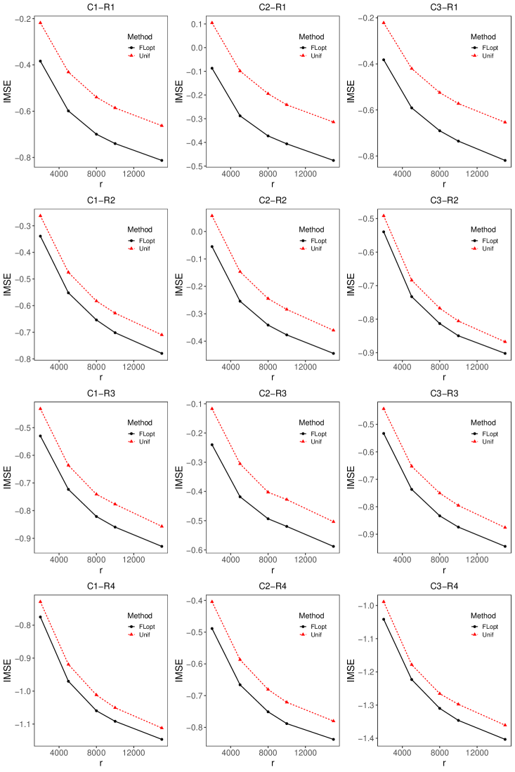
Figure 1: IMSE for different subsampling sizes $r$ and fixed first step subsampling size $r_{0}=1000$ with different distributions when $n=10^{5}$.

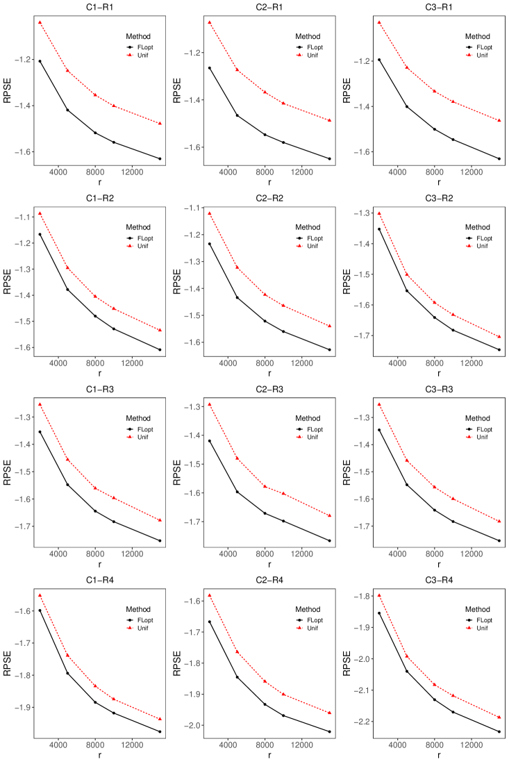
Figure 2: RPSE for different subsampling sizes $r$ and fixed first step subsampling size $r_{0}=1000$ with different distributions when $n=10^{5}$.

To evaluate the computational efficiency of the subsampling methods, we record the computing time of each method used in the case C1-R1 on a PC with an Intel I5 processor and 8GB memory using R, where the time required to generate the data is not included. We set $n=10^{6}$, $r_{0}=200$ and enlarge the number of knots for spline function to $K=50$. Each subsampling strategy is evaluated 100 times. The results on different $r$ with a fixed $\lambda$ for the FLopt and Unif subsampling methods are given in Table 3. It is clear that subsampling can significantly improve computational efficiency compared with full data, and the FLopt method is more expensive than the Unif method as expected.

Table 3: CPU seconds for different subsampling sizes $r$ with $n=10^{6}$, $r_{0}=200$, $K=50$ and a fixed $\lambda$. The times are the mean times calculated from 100 implementations of each method.

Method	$r$
	1000	2000	3000	4000	5000
FLopt	0.6036	0.6101	0.6230	0.6298	0.6393
Unif	0.0142	0.0250	0.0355	0.0455	0.0554
Full data CPU seconds: 11.8155

5 Real data analysis

5.1 Tecator data

Tecator data is available in fda.usc package, which has 215 meat samples. For each sample, the data consists of 100 channel spectrum of absorbance and the contents of fat, water and protein which are measured in percent. The 100 channel spectrum measured over the wavelength range 850-1050nm provides a dense measurement spaced 2nm apart that can be considered functional data. Figure 3 shows 50 randomly selected curves of spectrum of absorbance and the histogram of the content of protein. In this experiment, we shall study protein content by our proposed FLPRE.

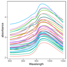
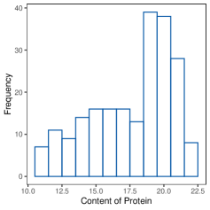
Figure 3: Left subfigure: A random subset of 50 spectrometric curves. Right subfigure: Histogram of the content of protein.

We employ the first 160 observations to fit the model, and then apply the remaining samples to evaluate the prediction efficiency by the mean of absolute prediction errors (MAPE) and product relative prediction errors (MPPE). The two mean criteria are measured by:

$$\mathrm{MAPE}=\frac{1}{55}\sum_{i=161}^{215}\lvert y_{i}-\hat{y}_{i}\rvert;$$

$$\mathrm{MPPE}=\frac{1}{55}\sum_{i=161}^{215}(y_{i}-\hat{y}_{i})^{2}/(y_{i}\hat{y}_{i}),$$

where $\hat{y}_{i}=\exp(\int_{0}^{1}x_{i}(t)\hat{\beta}(t)\mathrm{d}t)$. All results are presented in Table 4 which illustrates that the proposed FLPRE outperforms FLS and FLAD for predicting the protein content.

Table 4: MAPE and MPPE for Tecator data.

Criterion	FLS	FLAD	FLPRE
MAPE	3.5836	3.7452	3.5420
MPPE	0.0745	0.0739	0.0727

5.2 Beijing multi-site air-quality data

This data set is available in https://archive-beta.ics.uci.edu/ml/datasets/beijing+multi+site+air+quality+data, and consists of hourly air pollutants data from 12 nationally controlled air-quality monitoring sites in Beijing from March 1, 2013 to February 28, 2017. Our primary interest here is to predict the maximum of daily $\mathrm{PM}_{10}$ concentrations ($\mu g/m^{3}$) using the $\mathrm{PM}_{10}$ trajectory (24 hours) of the last day. We delete all missing values and obtain a sample of 15573 days’ complete records. We take the top 80$\%$ of the sample as the training set and the rest as the test set. The raw observations after the square-root transformation are first transformed into functional data using 15 Fourier basis functions. This transformation can be implemented with the Data2fd function in the fda package, suggested in Sang and Cao (2020). A random subset of 100 curves of 24-hourly $\mathrm{PM}_{10}$ concentrations is presented in the left panel of Figure 4, where the time scale has been transformed to $[0,1]$. The right panel of Figure 4 depicts the histogram of the maximal values of intraday $\mathrm{PM}_{10}$ concentrations.

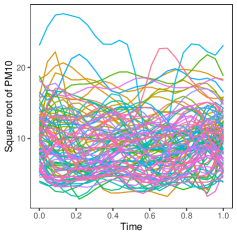
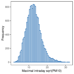
Figure 4: Left subfigure: A random subset of 100 curves of 24-hourly $\mathrm{PM}_{10}$ concentrations. Right subfigure: Histogram of the maximal values of intraday $\mathrm{PM}_{10}$ concentrations.

We assess the performances of prediction by the MAPE and MPPE criteria. Table 5 illustrates that the proposed FLPRE outperforms FLS and FLAD for predicting the $\mathrm{PM}_{10}$ concentrations.

Table 5: MAPE and MPPE for the air-quality data.

Criterion	FLS	FLAD	FLPRE
MAPE	7.9902	8.7580	7.6727
MPPE	0.5031	0.5223	0.4970

Further, we calculate the IMSE and RPSE using (4.2) and compare the FLopt method with the Unif method. Figure 5 shows the results for different subsampling sizes $r=1000,1500,2000,2500,3000$ with $r_{0}=1000$. We can find that the FLopt method always has smaller IMSE and RPSE compared with the Unif method. Besides, all IMSE and RPSE gradually decrease as the subsampling size $r$ increases, showing the estimation consistency of the subsampling methods and better approximation to the results based on full data.

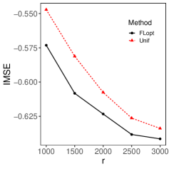
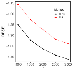
Figure 5: IMSE and RPSE for different subsampling sizes $r$ with $r_{0}=1000$ for 1000 repetitions.

Supplementary Materials

All technical proofs are included in the online Supplementary Material.

Qian Yan
College of Mathematics and Statistics, Chongqing University, Chongqing 401331, China. E-mail: qianyan@cqu.edu.cn

Hanyu Li
College of Mathematics and Statistics, Chongqing University, Chongqing 401331, China. E-mail: lihy.hy@gmail.com or hyli@cqu.edu.cn

References

- Ai et al. (2021a) Ai M., Wang F., Yu J. and Zhang H. (2021a). Optimal subsampling for large-scale quantile regression. Journal of Complexity 62, 101512.
- Ai et al. (2021b) Ai M., Yu J., Zhang H. and Wang H. (2021b). Optimal subsampling algorithms for big data regression. Statistica Sinica 31, 749–772.
- Atkinson, Donev and Tobias (2007) Atkinson A., Donev A. N. and Tobias R. D. (2007) Optimum Experimental Designs, with SAS. Oxford University Press, New York.
- Cardot, Ferraty and Sarda (2003) Cardot H., Ferraty F. and Sarda P. (2003). Spline estimators for the functional linear model. Statistica Sinica 13, 571–591.
- Chen et al. (2010) Chen, K., Guo S., Lin Y. and Ying Z. (2010). Least absolute relative error estimation. Journal of the American Statistical Association 105, 1104–1112.
- Chen et al. (2016) Chen K., Lin Y., Wang Z. and Ying Z. (2016). Least product relative error estimation. Journal Of Multivariate Analysis 144, 91–98.
- Chen and Liu (2021) Chen Y. and Liu H. (2021). A new relative error estimation for partially linear multiplicative model. Communications in Statistics-Simulation and Computation, 1–19.
- Chen, Liu and Ma (2022) Chen Y., Liu H. and Ma J.(2022). Local least product relative error estimation for single-index varying-coefficient multiplicative model with positive responses. Journal of Computational and Applied Mathematics 415, 114478.
- Claeskens, Krivobokova and Opsomer (2009) Claeskens G., Krivobokova T. and Opsomer J. D. (2009). Asymptotic properties of penalized spline estimators. Biometrika 96, 529–544.
- de Boor (2001) de Boor C. (2001). A Practical Guide to Splines. Springer-Verlag, Berlin.
- Fan, Zhang and Wu (2022) Fan, R., Zhang S. and Wu Y. (2022). Penalized relative error estimation of functional multiplicative regression models with locally sparse properties. Journal of the Korean Statistical Society 51, 666–691.
- Fan, Liu and Zhu (2021) Fan Y., Liu Y. and Zhu L. (2021). Optimal subsampling for linear quantile regression models. Canadian Journal of Statistics 49, 1039–1057.
- He and Yan (2022) He S., Yan X. (2022). Functional principal subspace sampling for large scale functional data analysis. Electronic Journal of Statistics 16,2621–2682.
- Liu, You and Cao (2021) Liu H., You J. and Cao J. (2021). Functional L-optimality subsampling for massive data. arXiv preprint arXiv:2104.03446.
- Ma, Mahoney and Yu (2015) Ma P., Mahoney M. W. and Yu B. (2015). A statistical perspective on algorithmic leveraging. Journal of Machine Learning Research 16, 861–911.
- Ma et al. (2020) Ma P., Zhang X., Xing X., Ma J. and Mahoney M. W. (2020). Asymptotic analysis of sampling estimators for randomized numerical linear algebra algorithms. In Proceedings of the Twenty Third International Conference on Artificial Intelligence and Statistics, 1026–1035.
- Ming, Liu and Yang (2022) Ming H., Liu H. and Yang H. (2022). Least product relative error estimation for identification in multiplicative additive models. Journal of Computational and Applied Mathematics 404, 113886.
- Ren, Zhao and Wang (2022) Ren M., Zhao S. and Wang M. (2022). Optimal subsampling for least absolute relative error estimators with massive data. Journal of Complexity 74, 101694.
- Ruppert (2002) Ruppert D. (2002) Selecting the number of knots for penalized splines. Journal of Computational and Graphical Statistics 11, 735–757.
- Sang and Cao (2020) Sang P. and Cao J. (2020). Functional single-index quantile regression models. Statistics and Computing 30, 771–781.
- Shao, Song and Zhou (2022) Shao L., Song S. and Zhou Y. (2022). Optimal subsampling for large-sample quantile regression with massive data. Canadian Journal of Statistics. https://doi.org/10.1002/cjs.11697
- Shao and Wang (2021) Shao Y. and Wang L. (2021). Optimal subsampling for composite quantile regression model in massive data. Statistical Papers 63, 1139–1161.
- Wang (2019) Wang H. (2019). More efficient estimation for logistic regression with optimal subsamples. Journal of Machine Learning Research 20, 1–59.
- Wang and Ma (2021) Wang H. and Ma Y. (2021). Optimal subsampling for quantile regression in big data. Biometrika 108, 99–112.
- Wang, Zhu and Ma (2018) Wang H., Zhu R. and Ma P. (2018). Optimal subsampling for large sample logistic regression. Journal of the American Statistical Association 113, 829–844.
- Wang and Zhang (2022) Wang T. and Zhang H. (2022). Optimal subsampling for multiplicative regression with massive data. Statistica Neerlandica 76, 418–449.
- Yao and Wang (2019) Yao Y. and Wang H. (2019). Optimal subsampling for softmax regression. Statistical Papers 60, 585–599.
- Yan, Li and Niu (2022) Yan Q., Li H. and Niu C. (2022). Optimal subsampling for functional quantile regression. Statistical Papers. https://doi.org/10.1007/s00362-022-01367-z.
- Yu, Wang and Ai (2020) Yu J., Wang H., Ai M. and Zhang H. (2020). Optimal distributed subsampling for maximum quasi-likelihood estimators with massive data. Journal of the American Statistical Association 117, 265–276.
- Yuan et al. (2022) Yuan X., Li Y., Dong X. and Liu T. (2022). Optimal subsampling for composite quantile regression in big data. Statistical Papers 63, 1649–1676.
- Zhang et al. (2019) Zhang T., Huang Y., Zhang Q., Ma S. and Ahmed S. E. (2019). Penalized relative error estimation of a partially functional linear multiplicative model. In Ahmed S. E., Carvalho F. and Puntanen S. (Eds.), Matrices, Statistics and Big Data, Springer, Cham.
- Zhang, Zhang and Li (2016) Zhang T., Zhang Q. and Li N. (2016). Least absolute relative error estimation for functional quadratic multiplicative model. Communications in Statistics-Theory and Methods 45, 5802–5817.