Further Improving Weakly-supervised Object Localization via Causal Knowledge Distillation

Abstract

Weakly-supervised object localization aims to indicate the category as well as the scope of an object in an image given only the image-level labels. Most of the existing works are based on Class Activation Mapping (CAM) and endeavor to enlarge the discriminative area inside the activation map to perceive the whole object, yet ignore the co-occurrence confounder of the object and context (e.g., fish and water), which makes the model inspection hard to distinguish object boundaries. Besides, the use of CAM also brings a dilemma problem that the classification and localization always suffer from a performance gap and can not reach their highest accuracy simultaneously. In this paper, we propose a casual knowledge distillation method, dubbed KD-CI-CAM, to address these two under-explored issues in one go. More specifically, we tackle the co-occurrence context confounder problem via causal intervention (CI), which explores the causalities among image features, contexts, and categories to eliminate the biased object-context entanglement in the class activation maps. Based on the de-biased object feature, we additionally propose a multi-teacher causal distillation framework to balance the absorption of classification knowledge and localization knowledge during model training. Extensive experiments on several benchmarks demonstrate the effectiveness of KD-CI-CAM in learning clear object boundaries from confounding contexts and addressing the dilemma problem between classification and localization performance.

1 Introduction

Object localization schneiderman2004object ; bergtholdt2010study ; tompson2015efficient ; choudhuri2018object aims to indicate the category and the scope of an object in a given image, in forms of bounding box everingham2010pascal ; russakovsky2015imagenet ; liu2020deep . This task has been studied extensively in the computer vision community tompson2015efficient ; song2021weakly due to its broad applications, such as medical diagnosis ruppertshofen2013discriminative ; alaskar2022deep and autonomous driving behl2017bounding ; shekar2021label . Recently, the techniques based on deep convolutional neural networks (DCNNs) simonyan2014very ; szegedy2015going ; he2016deep ; luo2021category ; luo2018macro promote the localization performance to a new level. However, this performance promotion is at the price of huge amounts of fine-grained human annotationsluo2019taking ; luo2020ASM ; chan2021comprehensive ; shao2022active . To alleviate such a heavy burden, weakly-supervised object localization (WSOL) has been proposed by only resorting to image-level labels.

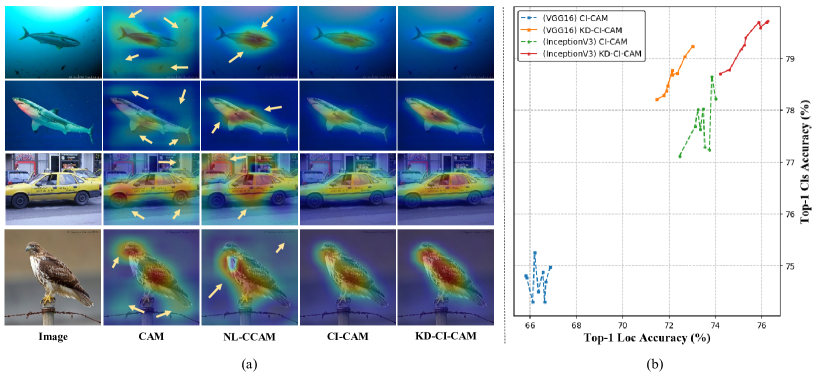
Figure 1: (a) Visualization comparison between vanilla CAM, NL-CCAM, CI-CAM, and KD-CI-CAM. The yellow arrows indicate the regions suffer from entangled contexts. (b) The classification-localization dilemma faced by prior CAM-based methods (e.g., CI-CAM), where the classification and localization suffer from a performance gap and can not achieve their highest accuracy simultaneously.

To capitalize on the image-level labels, the existing studies selvaraju2017grad ; diba2017weakly ; kim2017two ; wei2018ts2c ; shao2022deep ; shao2021improving follow the Class Activation Mapping (CAM) approach zhou2016learning to generate class activation maps first and then segment the highest activation area for a coarse localization. Albeit, CAM is initially designed for the classification task and tends to focus only on the most discriminative feature to increase its classification accuracy. To deal with this issue, recent prevailing works diba2017weakly ; kim2017two ; wei2018ts2c ; zhang2018adversarial ; gao2019c ; mai2020erasing ; yang2020combinational endeavor to perceive the whole objects instead of the shrunken and sparse “discriminative regions”. On one hand, they refine the network structure to make the detector more tailored for object localization in a weak supervision setting. For example, some methods diba2017weakly ; wei2018ts2c use a three-stage structure to continuously optimize the prediction results by training the current stage using the output of the previous stages as supervision. Other works kim2017two ; zhang2018adversarial ; gao2019c ; mai2020erasing leverage two parallel branches where the first branch is designed for digging out the most discriminative small regions while the second one is responsible for detecting the less discriminative large regions. On the other hand, they also make full use of the image information to improve the prediction results. For instance, $TS^{2}C$ wei2018ts2c and NL-CCAM yang2020combinational utilize the contextual information of surrounding pixels and the activation maps of low probability class, respectively.

Although the works along the vein of CAM have led to some impressive early results, we have discovered multi-faceted problems that remain unexplored by those prior arts, which emerged from our experimental analysis. Firstly, vanilla CAM mechanism is incapable of reasoning about the co-occurrence confounder (e.g., fish and water) in the images, which makes the model inspection hard to distinguish between the object and context and causes biased activation maps, as shown in Figure 1 (a). We dub this problem as “entangled context” for convenience. Secondly, we noticed that the classification and localization always suffer from a performance gap and can not reach their highest accuracy simultaneously in previous CAM-based methods. Taking CI-CAM shao2021improving as an example, we set up multiple independent experiments using different training settings, however, none of the results can achieve the best classification and localization performance at the same time, as reported in Figure 1 (b). We summarise this issue as a classification-localization dilemma (“C-L dilemma” for short). We argue that these two problems severely hinder the WSOL performance and heretofore yet to be well studied, despite the existence of a vast body of WSOL literature zhou2016learning ; diba2017weakly ; zhang2018adversarial ; zhang2020inter ; mai2020erasing ; wei2021shallow ; wu2022background .

Taking one step further into these two issues, we found the internal reasons behind them are different. The “entangled context” derives from the fact that objects usually co-occur with a certain context background, e.g., the most “fish” appears concurrently with “water” in the images. Consequently, these two concepts would be inevitably entangled and a classification model would wrongly generate an ambiguous boundary between “fish” and “water” with image-level supervision. In contrast to the vanilla CAM which yields a relatively shrunken bounding box on the small discriminative region, we notice that the “entangled context” problem would cause a biased expanding bounding box that includes the wrongly entangled background, which impairs the localization accuracy in terms of the object range. While the “C-L dilemma” is derived from a hallmark of a classification network that tends to focus on discriminative region information (e.g., the head of an animal) over the integral profile of an object to better distinguish various categories. Forcing a classification model to pay more attention to the unrepresentative area (e.g., the fur of an animal) conceding to the integral contour perception would inevitably cause a biased categorical prediction, and vise versa for a localization model. Prior approaches sidestep such a dilemma by simply trading off the classification and localization performances, i.e., choosing a mutually acceptable model or only reporting localization results pan2021unveiling ; wu2022background ; kim2022bridging ; xu2022cream . However, the intrinsic issue behind this dilemma remains under-explored.

In this paper, we propose a casual knowledge distillation framework to solve both “entangled context” and “C-L dilemma” problems in one go, dubbed KD-CI-CAM. Specifically, we first explore the causalities among image features, contexts, and labels by establishing a structural causal model (SCM) pearl2016causal and pinpoint the context as a confounder as shown in Figure 2. According to the causal analysis, we propose a causal context pool to eliminate the biased co-occurrence in the class activation maps to solve the “entangled context” problem as shown in Figure 3. Based on disentangled object features from the wrongly contextual information, we further tackle the “C-L dilemma” problem faced by the CAM-based model via a multi-teacher causal distillation framework as shown in Figure 4. The first kind of teacher focuses on classification, which aims to provide good logit knowledge. The other one is a localization teacher, which is responsible for providing high-quality class activation map knowledge. These two teachers endow our student model with the ability to balance the absorption of classification knowledge and localization knowledge. To prevent the degradation of knowledge transfer from the model capacity gap between the student and teachers mirzadeh2020improved ; gao2021residual , these teachers adopt the same network structure with the student except for their objective loss functions. With these tailored designs, KD-CI-CAM can not only effectively eliminate the spurious correlations between pixels and labels from the “entangled context” problem, but also alleviates the “C-L dilemma” problem resulting from the interesting bias between the classification information and localization information.

It is noteworthy that some pertinent results of this work have been published in an earlier version shao2021improving . This paper goes beyond shao2021improving by contributing to introducing a novel casual knowledge distillation framework to further boost the WSOL by solving the notorious but under-explored “entangled context” and “C-L dilemma” problems in one go. We also make significant improvements in experimental validation and analysis compared to the early version.

Generally, the contributions of this paper can be summarized as follows:

• We are among the pioneers to concern and reveal the “entangled context” problem and “C-L dilemma” problem of WSOL that remain unexplored by prevailing efforts.

• We propose a novel casual knowledge distillation method, dubbed KD-CI-CAM, to solve the under-explored “entangled context” and “C-L dilemma” problems in one go. We first design a student model by using causal intervention to address the confounder context, and then balance its absorption of classification knowledge and localization knowledge by using a knowledge distillation framework.

• Extensive experiments show that both “entangled context” and “C-L dilemma” problems are effectively solved by our proposed methods.

2 Related Work

2.1 Weakly-supervised Object Localization

Since CAM zhou2016learning is prone to bias to the most discriminative part of the object rather than the integral object, the research attention of most of the current methods is how to improve the accuracy of object localization. These methods can be broadly categorized into two groups: enlarging the proposal region and discriminative region removal.

1) Enlarging proposal region: enlarging the box size appropriately of the initial prediction box diba2017weakly ; wei2018ts2c . WCCN diba2017weakly introduces three cascaded networks trained in an end-to-end pipeline. The latter stage continuously enlarges and refines the output proposals of its previous stage. $TS^{2}C$ wei2018ts2c selects the box by comparing the mean pixel confidence values of the initial prediction region and its surrounding region. If the gap between the mean values of the two regions is large, the initial prediction region is the final prediction box; otherwise, the surrounding region.

2) Discriminative region removal: detecting the bigger region after removing the most discriminative region kim2017two ; zhang2018adversarial ; choe2019attention ; mai2020erasing . TP-WSL kim2017two first detects the most discriminative region in the first network, Then, it erases this region of the conv5-3 feature maps in the second network (e.g., zero). ACoL zhang2018adversarial uses the masked feature maps by erasing the most discriminative region discovered in the first classifier as the input feature maps of the second classifier. ADL choe2019attention stochastically produces an erased mask or an importance map at each iteration as a final attention map projected in the feature maps of images. MEIL mai2020erasing is an adversarial erasing method that simultaneously computes the erased branch and the unerased branch by sharing one classifier.

The above methods basically focus on the poor localization caused by the most discriminative part of the object. However, they ignore the problem of the fuzzy boundary between the objects and the co-occur certain context background. For example, if most “fish” appears concurrently with “water” in the images, these two concepts would be inevitably entangled and wrongly generate ambiguous boundaries using only image-level supervision.

2.2 Causal Inference

Structural Causal Model (SCM) pearl2016causal is an important analysis tool in causal inference scenes yue2020interventional ; zhang2020causal ; tang2020long , which is a directed graph in which each node represents each participant of the model, and each link denotes the causalities between the two nodes zhang2020causal . Specifically, Zhang et al. zhang2020causal utilize a SCM didelez2001judea ; pearl2016causal to deeply analyze the causalities among image features, contexts, and class labels and propose Context Adjustment (CONTA) that achieves the new state-of-the-art in weakly-supervised semantic segmentation task. Yue et al. yue2020interventional use the causal intervention in few-shot learning and uncover the pre-trained knowledge is indeed a confounder that limits the performance. Finally, they propose a novel FSL paradigm: Interventional Few-Shot Learning (IFSL). Tang et al. tang2020long show the SGD momentum is essentially a confounder in long-tailed classification by using a SCM.

Inspired by CONTA zhang2020causal , we also leverage a SCM pearl2016causal to analyze the causalities among image features, contexts, and class labels and find context is a confounder factor in §3.2.1. But, our work does not follow the strategy of alternating training of multiple models. Instead, we propose an end-to-end model embedding the causal inference into the WSOL pipeline, which is capable of making the feature boundary clearer by using a causal context pool in §3.2.3.

2.3 Knowledge Distillation

Knowledge distillation hinton2015distilling ; wu2020learning ; gou2021knowledge aims to transfer knowledge from the cumbersome teacher model to a small student model. It can be categorized into two parts: knowledge and distillation. First, knowledge can be grouped into response-based knowledge hinton2015distilling and feature-based knowledge zheng2022localization . The response-based knowledge refers to the prediction logits, which are simple yet effective in the distillation of the classification task. However, using only the teacher’s logits information in complex distillation is insufficient. Thus, researchers pay attention to utilizing feature-based knowledge to boost the effect of distillation in complex scenes. Second, distillation is the mode of transferring the knowledge from the teacher model to the student model, which also can be divided into offline distillation huang2017like ; heo2019knowledge , online distillation chen2020online ; wu2021peer , and self-distillation lan2018self ; yun2020regularizing ; zhao2021soda . To make the student model learn knowledge smoothly, it usually adopts a “soft target”—using a “softmax” with a temperature $T$ on the knowledge of teachers, as the extra supervision of the student model.

In this work, to harness the absorption of classification and localization knowledge in the CAM-based model, we derive a multi-teacher causal distillation framework. The classification knowledge and localization knowledge are selected stochastically at each distillation process to supervise the learning of the student, which will be detailed in §3.3.

3 Methodology

In this section, we first introduce the preliminaries of problem settings and baseline method in §3.1. Then we will concentrate on solving the “entangled context” issue and propose our causal intervention method in §3.2. Based on the casual model, we finally tackle the “C-L dilemma” problem and construct the multi-teacher casual distillation framework (KD-CI-CAM) in §3.3.

3.1 Preliminaries

3.1.1 Problem Settings

Before presenting our method, we first introduce the problem settings of WSOL formally. Given an image $I$, WSOL targets classifying and locating one object in terms of the class label and the bounding box. However, only image-level labels $Y$ can be accessed during the training phase.

3.1.2 Baseline Method

Class activation maps (CAMs) are widely employed for generating the object boxes in the WSOL task. Yang et al. yang2020combinational argue that using only one activation map of the highest probability class for segmenting object boxes is problematic since it often biases to over-small regions or sometimes even highlights background area. Based on such observation, they propose the NL-CCAM yang2020combinational method to combine all activation maps from the highest to the lowest probability class to a localization map using a specific combinational function and achieve good localization performance.

Based on the vanilla fully convolutional network (FCN)-based backbone, e.g., VGG16 simonyan2014very , NL-CCAM yang2020combinational inserts four non-local blocks before every bottleneck layer excluding the first bottleneck layer simultaneously to produce a non-local fully convolutional network (NL-FCN). Given an image $I$, it is fed into the NL-FCN to produce its feature maps $X\in\mathbb{R}^{c\times h\times w}$, where $c$ is the number of channels and ${h\times w}$ is the spatial size. Then, the feature maps $X$ are forwarded to a global average pooling (GAP) layer followed by a classifier with a fully connected layer. The prediction scores $S=\{s_{1},s_{2},\ldots,s_{n}\}$ are computed by using a softmax layer on the top of the classifier for classification. The weight matrix of the classifier is denoted as $W\in\mathbb{R}^{n\times c}$, where $n$ is the number of image classes. Thus, the activation maps $M_{i}$ of class $i$ among class activation maps (CAMs) $M\in\mathbb{R}^{n\times h\times w}$ proposed in zhou2016learning are given as follows.

$$M_{i}=\sum_{k}^{c}{W_{i,k}\cdot X_{k}},$$ (1)

where $i\in\{1,2,\ldots,n\}$.

NL-CCAM yang2020combinational produces a localization map by using a combinational function in CAMs instead of using the activation map of the highest probability class among CAMs. Firstly, it ranks the activation maps from the highest probability class to the lowest and uses $M_{t_{k}}$ to denote the activation map of the $k$ highest probability class. The class label with the highest probability $t_{1}$ is computed as follows.

$$t_{1}=argmax_{k}(\{S_{k}\}),$$ (2)

where $k\in\{1,2,\ldots,n\}$. Then it combines $M$ to a localization heatmap $H\in\mathbb{R}^{h\times w}$ as follows.

$$H=\sum_{k}^{n}\gamma(k)\cdot M_{k},$$ (3)

where $\gamma(\cdot)$ is a combinational function. Finally, it segments the localization heatmap $H$ using a threshold proposed in zhou2016learning to generate a bounding box for object localization.

Our method is based on NL-CCAM yang2020combinational but introduces substantial improvements. We not only equip the baseline network with the ability of causal inference to tackle the “entangled context” problem but also address the “C-L dilemma” problem suffered from the traditional CAM-based models.

3.2 Causal Intervention for Student Network

In this section, we target the “entangled context” problem. Specifically, we first reveal the reason why the confounder context hurts the object localization quality using a structural causal model pearl2016causal in §3.2.1. Then, we use the causal intervention to solve the “entangled context” problem theoretically via the backdoor adjustment pearl2016causal . Finally, we implement the causal module in our model in §3.2.3.

3.2.1 Structural Causal Model

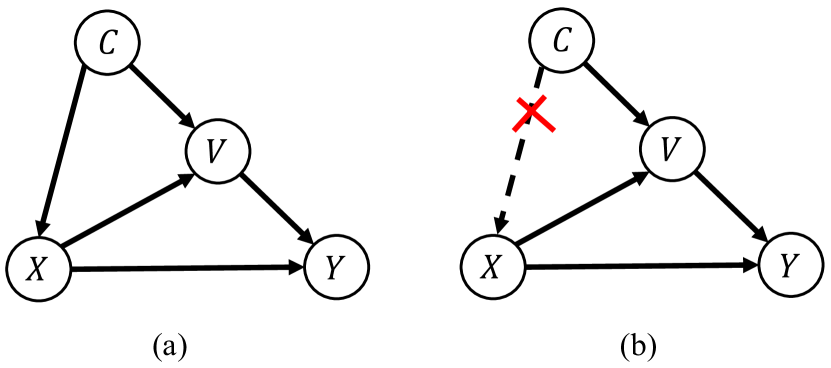
Figure 2: (a) Building the structural causal model (SCM) in WSOL. (b) Cutting off the confounding effect of $C\rightarrow X$ in WSOL. $X$: feature maps. $C$: confounder context. $V$: image representation. $Y$: image label.

Inspired by CONTA zhang2020causal , we utilize a structural causal model (SCM) pearl2016causal to analyze the causalities among image features $X$, confounder context $C$, and image-level labels $Y$. The direct links shown in Figure 2 (a) denote the causalities between the two nodes: cause $\rightarrow$ effect zhang2020causal .

$\bm{C\rightarrow X}$: This link indicates that the backbone generates feature maps $X$ under the effect of context $C$. Although the confounder context $C$ is helpful for a better association between the image features $X$ and labels $Y$ via a model $P(Y|X)$, e.g., it is likely a “fish” when perceiving a “water” region, $P(Y|X)$ mistakenly associates non-causal but positively correlated pixels to labels, e.g., the “water” region wrongly belongs to “fish”. This is a vital reason for the inaccurate localization in WSOL. Fortunately, as we will introduce later in §3.2.3, we can avoid it by using a causal context pool in causal intervention.

$\bm{C\rightarrow V\leftarrow X}$: $V$ is an image specific-representation using the contextual templates from $C$ zhang2020causal . For example, $V$ tells us the shape and location of a “fish” (foreground) in a scene (background) zhang2020causal . In this paper, $V$ denotes the activation map of the highest probability class in the CAM 1 module as shown in Figure 3.

$\bm{X\rightarrow Y\leftarrow V}$: These links indicate that image feature $X$ and image representation $V$ together affect the image label $Y$ of an image. We consider that the shape and location information of object instance contained in image representation $V$ also directly affects the image label $Y$. As a consequence, though $V$ is not an input factor in the WSOL model, it exists zhang2020causal .

3.2.2 Theoretical Analysis

To remove the confounding effect of $\bm{C\rightarrow X}$ as shown in Figure 2 (b), we take inspiration from CONTA zhang2020causal , following the same rule to use $P(Y|do(X))$ based on the backdoor adjustment pearl2016causal as the new image-level classifier. The key idea is that $X$ and $C=\{c_{1},c_{2},\ldots,c_{n}\}$ are independent events. As $C$ does not affect $X$, it guarantees $X$ to have a fair opportunity to incorporate every context $c$ into $Y$’s prediction, subject to a prior $P(c)$ zhang2020causal . Formally, we have the following probability formula:

$$P(Y|do(X)) =\sum_{i}^{n}P(Y|do(X),c_{i})\cdot P(c_{i}|do(X))$$ (4)

$$=\sum_{i}^{n}P(Y|X,c_{i})\cdot P(c_{i})$$

$$=\sum_{i}^{n}P(Y|X,c_{i},V)\cdot P(V|X,c_{i})\cdot P(c_{i})$$

$$=\sum_{i}^{n}P(Y|X,c_{i},V=f(X,c_{i}))\cdot P(c_{i})$$

$$=\sum_{i}^{n}P(Y|X,V=f(X,c_{i}))\cdot P(c_{i})$$

$$=\sum_{i}^{n}P(Y|X=x,V=f(x,c_{i}))\cdot P(c_{i}),$$

where $P(Y|do(X))=\sum_{i}^{n}P(Y|do(X),c_{i})\cdot P(c_{i}|do(X))$ follows the law of total probability. $n$ is the number of image classes. Since $X$ and $C=\{c_{1},c_{2},\ldots,c_{n}\}$ are independent events, $P(c_{i}|do(X))=P(c_{i})$. $f(X,c_{i})$ abstractly represents that $V$ is effected by $X$ and $c_{i}$, so $P(V|X,c_{i})=1$. Because $Y$ is only directly affected by $X$ and $V$ in Figure 2 (b), $P(Y|X,c_{i},V=f(X,c_{i}))=P(Y|X,V=f(X,c_{i}))$. Inspired by CONTA zhang2020causal , we adopt the NWGM xu2015show to optimize Eq. (4) by moving the outer sum $\sum_{i}^{n}P(c_{i})$ into the feature level

$$P(Y|do(X))\approx P(Y|X=x,V=\sum_{i}^{n}f(x,c_{i})\cdot P(c_{i})).$$ (5)

Since the number of samples for each class in the dataset is roughly the same, we set $P(c)$ to uniform $1/n$. After further optimizing Eq. (5), we have

$$P(Y|do(X))\approx P(Y|x\oplus\frac{1}{n}\cdot\sum_{i}^{n}f(x,c_{i})),$$ (6)

where $\oplus$ denotes projection. So far, the “entangled context” issue has been transferred into calculating $\sum_{i}^{n}f(x,c_{i})$. We will introduce a causal context pool $Q$ to represent $\sum_{i}^{n}f(x,c_{i})$ in §3.2.3.

3.2.3 Student Network Architecture

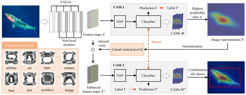
Figure 3: Overview of the proposed CI-CAM (Student network). CI-CAM consists of four parts: a backbone to extract the feature maps, the share-weighted CAM modules to generate the class activation maps, a causal context pool (which is the core of the CI-CAM method) to enhance the feature maps by eliminating the negative effect of confounder, and a combinational module to generate the final bounding box.

We implement a causal model for the “entangled context” problem, dubbed CI-CAM, at the core of which is a causal context pool. The main idea of the causal context pool is to accumulate all contexts of each class, and then re-project the contexts to the feature maps of convolutional layers shown in Eq. (6) to pursue the pure causality between the cause $X$ and the effect $Y$. Figure 3 illustrates the overview of CI-CAM that includes four parts: backbone, CAM module, causal context pool, and combinational part.

Backbone. Inherited from the baseline method, we design our backbone by inserting multiple non-local blocks at both low- and high-level layers of a FCN-based network simultaneously. It acts as a feature extractor that takes the RGB images as input and produces high-level position-aware feature maps.

CAM module. It includes a global average pooling (GAP) layer and a classifier with a fully connected layer zhou2016learning . Image feature maps $X$ generated by the backbone are forwarded into GAP and classifier to produce prediction scores $S=\{s_{1},s_{2},\ldots,s_{n}\}$. The CAM network multiplies the weight $W$ of the classifier to $X$ to produce class activation maps $M\in\mathbb{R}^{n\times h\times w}$ shown in Eq. (1). In our model, we use two CAM modules with shared weights. The first CAM module is designed to produce initial prediction scores $S$ and class activation maps $M$, and the second CAM network is responsible for producing more accurate prediction scores $S^{e}=\{s_{1}^{e},s_{2}^{e},\ldots,s_{n}^{e}\}$ and class activation maps $M^{e}\in\mathbb{R}^{n\times h\times w}$ using the feature maps $X^{e}\in\mathbb{R}^{c\times h\times w}$ enhanced by the causal context pool.

Causal context pool. We maintain a causal context pool $Q\in\mathbb{R}^{n\times h\times w}$ during the network training phase, where $Q_{i}$ denotes the context of all $i^{th}$ class images. $Q$ ceaselessly stores all contextual information maps (e.g., $V$) of each class by accumulating the activation map of the highest probability class. Then, it projects all contexts of each class as attention onto the feature maps of the last convolutional layer to produce enhanced feature maps. The idea behind using a causal context pool is not only to cut off the negative effect of entangled context on image feature maps but also to spotlight the positive region of the image feature maps for boosting localization performance.

Combinational part. The input of the combinational part is class activation maps $M^{e}$ generated from the CAM 2 module, and the corresponding output is a localization heatmap $H\in\mathbb{R}^{h\times w}$ calculated by Eq. (3): First, the combinational part ranks the activation maps from the highest probability class to the lowest. Second, it combines these sorted activation maps by a combinational function as Eq. (3).

With all the key modules presented above, we would give a brief illustration of the data flow in our network. Given an image $I$, we first forward $I$ to the backbone to produce feature maps $X$. $X$ is then fed into the following two parallel CAM branches. The first CAM branch produces initial prediction scores $S$ and class activation maps $M$. Then, the causal context pool $Q$ would be updated by fusing the activation map of the highest probability class in $M$ as follows:

$$Q_{\pi}=bn(Q_{\pi}+\lambda\cdot bn(V)),V=M_{\pi},$$ (7)

where $\pi=argmax(\{s_{1},s_{2},\ldots,s_{n}\})$, $\lambda$ denotes the update rate, and $bn$ denotes the batch normalization. The second branch is responsible for producing more accurate prediction scores $S^{e}$ and class activation maps $M^{e}$. The input of the second branch is enhanced feature maps $X^{e}$ projected by the context among causal context pool $Q$ of the highest probability class generated from the first branch. More concretely, the feature enhancement can be calculated as

$$X^{e}=X+X\odot Conv_{1\times 1}(Q_{\pi}),$$ (8)

where $\odot$ denotes the matrix dot product. In the combinational part, we first build a localization heatmap $H\in\mathbb{R}^{h\times w}$ by aggregating all activation maps from the highest to the lowest probability class using a specific combinational function yang2020combinational in Eq. (3). Then, we use the simple thresholding technique proposed by zhou2016learning to generate a bounding box $B$ from the localization map. Finally, the bounding box $B$ and prediction scores $S^{e}$ as the final prediction of CI-CAM.

3.2.4 Student Network Training Objective

During the phase of training, our proposed student network learns to minimize image classification losses for both classification branches. Given an image $I$, we can obtain initial prediction scores $S=\{s_{1},s_{2},\ldots,s_{n}\}$ and more accurate prediction scores $S^{e}=\{s_{1}^{e},s_{2}^{e},\ldots,s_{n}^{e}\}$ of the two classifiers as shown in Figure 3. We follow a naive scheme to train the two classifiers together in an end-to-end pipeline using the following loss function $\mathcal{L}^{stu}$ (Stu Loss).

$$\mathcal{L}^{stu}=\rho\cdot\left(-\sum_{i=1}^{n}y_{i}\cdot log(s_{i})\right)+\left(-\sum_{i=1}^{n}y_{i}\cdot log(s_{i}^{e})\right),$$ (9)

where $y$ is the ground-truth label of an image. If Stu Loss $\mathcal{L}^{stu}$ is used in Eq. 19 and Eq. 21, $\rho=1$; otherwise, $\rho=0$.

3.3 Multi-Teacher Causal Knowledge Distillation

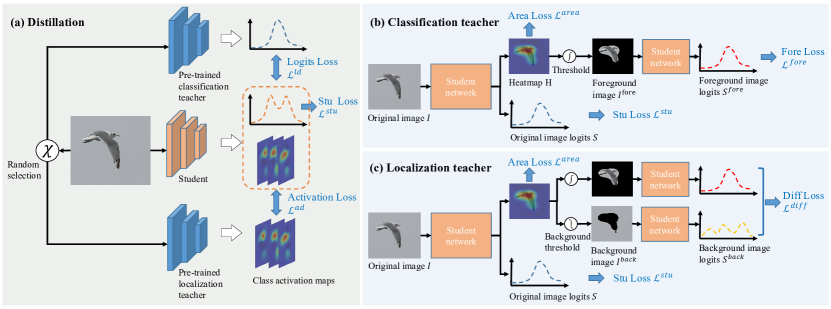
Figure 4: Overview of the multi-teacher causal distillation framework. (a) The classification teacher and localization teacher are applied stochastically during each distillation. (b) The classification teacher adopts the student network as its model structure but adds Area Loss and Fore Loss. The two orange student networks in the classification teacher are the same model. (c) The localization teacher uses the student network as its model structure but adds Area Loss and Diff Loss. The three orange student networks in the localization teacher are the same model.

3.3.1 Distillation Framework

To make the model simultaneously retain good classification performance and localization performance, we design a multi-teacher causal distillation framework that randomly selects the knowledge of the pre-trained classification teacher and localization teacher to supervise the learning of our student as shown in Figure 4 (a).

First, the pre-trained classification teacher provides logit knowledge to help the student network to achieve good classification performance. Inspired by hinton2015distilling , we design our logits distillation loss function $\mathcal{L}^{ld}$ between classification teacher and student as follows.

$$\mathcal{L}^{ld}=KL(\tilde{Z}^{stu},\tilde{Z}^{cls\_tch}),$$ (10)

$$\tilde{Z}^{stu}_{i}=\frac{\exp(Z^{stu}_{i}/T^{cls})}{\sum_{j=1}^{n}\exp(Z^{stu}_{j}/T^{cls})},$$ (11)

$$\tilde{Z}^{cls\_tch}_{i}=\frac{\exp(Z^{cls\_tch}_{i}/T^{cls})}{\sum_{j=1}^{n}\exp(Z^{cls\_tch}_{j}/T^{cls})},$$ (12)

where $KL$ is the Kullback-Leibler divergence function. $Z^{stu}$ and $Z^{cls\_tch}$ respectively denote the output logits $Z\in\mathbb{R}^{n}$ of the student network and the classification teacher network. $n$ is the number of classes and $i\in\{1,2,\ldots,n\}$. $T^{cls}$ is the logits distillation temperature.

Second, the pre-trained localization teacher brings the localization knowledge in the class activation maps to help the student network to accurately localize the whole object rather than the most discriminative part of the object. We design the activation distillation loss function $\mathcal{L}^{ad}$ between localization teacher and student as follows.

$$\mathcal{L}^{ad}=MSE(\tilde{A}^{stu},\tilde{A}^{loc\_tch}),$$ (13)

$$\tilde{A}^{stu}_{i}=\frac{\exp(A^{stu}_{i}/T^{loc})}{\sum_{j=1}^{nhw}\exp(A^{stu}_{j}/T^{loc})},$$ (14)

$$\tilde{A}^{loc\_tch}_{i}=\frac{\exp(A^{loc\_tch}_{i}/T^{loc})}{\sum_{j=1}^{nhw}\exp(A^{loc\_tch}_{j}/T^{loc})},$$ (15)

where $MSE$ is the Mean Squared Error function. $A^{stu}$ and $A^{loc\_tch}$ respectively denote the class activation maps $A\in\mathbb{R}^{nhw}$ of the student network and the localization teacher network. $h$ and $w$ are the height and width of the activation map. $T^{loc}$ is the activation distillation temperature. Finally, the total loss function $\mathcal{L}^{total}$ of the multi-teacher causal distillation framework in Figure 4 (a) is given as follows.

$$\mathcal{L}^{total}= \alpha\cdot[(\epsilon==1)\cdot\mathcal{L}^{ld}+(\epsilon==2)\cdot\mathcal{L}^{ad}]$$ (16)

$$+(1-\alpha)\cdot\mathcal{L}^{stu},$$

where $\alpha$ is the distillation strength hyper-parameter. $\epsilon\in\{0,1,2\}$ denotes the controller of the random selection in Figure 4 (a).

3.3.2 Classification Teacher Network

As shown in Figure 4 (b), to prevent the degradation of knowledge transfer from the model capacity gap between student and teacher mirzadeh2020improved ; gao2021residual , we adopt the same network structure with the student as our classification teacher but add two extra loss functions. Specifically, given an image $I$, it is first forwarded into the model to produce the original image logits $S=\{s_{1},s_{2},\ldots,s_{n}\}$ and localization heatmap $H\in\mathbb{R}^{h\times w}$, where $h$ and $w$ respectively denote the height and width of the original image $I$. Then, we obtain a binary foreground mask $M^{fore}$ by segmenting the heatmap $H$ using a threshold. Next, we generate a foreground image $I^{fore}$ by projecting the $M^{fore}$ into the original image $I$. Finally, $I^{fore}$ is fed into the model again to produce the foreground image logits $S^{fore}=\{s^{fore}_{1},s^{fore}_{2},\ldots,s^{fore}_{n}\}$.

To clearly distinguish the foreground area from the background area in heatmap $H$, we first introduce the Area Loss of xie2021online ; meng2021foreground to reduce the activation value of the foreground area and the background area in heatmap $H$. Then, we apply a Fore Loss to activate the object areas in the image by classifying the foreground image. As a result, Area Loss and Fore Loss terms together can suppress the background areas and highlight the foreground areas meng2021foreground . Area Loss $\mathcal{L}^{area}$ and Fore Loss $\mathcal{L}^{fore}$ are given as follows.

$$\mathcal{L}^{area}=\frac{1}{h\cdot w}\sum_{i=1}^{h}\sum_{j=1}^{w}H_{i,j},$$ (17)

$$\mathcal{L}^{fore}=-\sum_{i=1}^{n}y_{i}\cdot log(s_{i}^{fore}),$$ (18)

where $y$ is the ground-truth label of an image. Finally, our classification teacher learns to minimize the Area Loss $\mathcal{L}^{area}$, Fore Loss $\mathcal{L}^{fore}$, and Stu Loss $\mathcal{L}^{stu}$.

$$\mathcal{L}^{cls\_tch}=\mathcal{L}^{stu}+\mu\cdot\mathcal{L}^{fore}+\eta\cdot\mathcal{L}^{area},$$ (19)

where $\mathcal{L}^{cls\_tch}$ is the total loss of our classification teacher. $\mu$ and $\eta$ are the hyper-parameters.

3.3.3 Localization Teacher Network

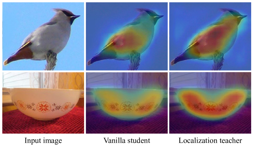
Figure 5: Visualization comparison between vanilla student (without knowledge distillation) and localization teacher.

As shown in Figure 4 (c), similar to the classification teacher network, we also use the same network structure with the student as our localization teacher but add two extra loss functions. Given an image $I$, it is first forwarded into the model to produce the original image logits $S=\{s_{1},\ldots,s_{n}\}$ and localization heatmap $H\in\mathbb{R}^{h\times w}$, where $h$ and $w$ respectively denote the height and width of the original image $I$. Then, we respectively obtain the binary foreground mask $M^{fore}$ and background mask $M^{back}$ by segmenting the heatmap $H$ using a threshold. Next, we generate the foreground image $I^{fore}$ and background image $I^{back}$ by respectively projecting the $M^{fore}$ and $M^{back}$ into the original image $I$. Finally, the foreground image $I^{fore}$ and background image $I^{back}$ are fed into the model again to yield the foreground image logits $S^{fore}=\{s^{fore}_{1},s^{fore}_{2},\ldots,s^{fore}_{n}\}$ and background image logits $S^{back}=\{s^{back}_{1},\ldots,s^{back}_{n}\}$, respectively.

To make the foreground image contain the integral object as much as possible while reducing the object information in the background area, we design a difference loss (Diff Loss) $\mathcal{L}^{diff}$, which is given as follows.

$$\mathcal{L}^{diff}= -\sum_{i=1}^{n}y_{i}\cdot log(s_{i}^{fore}-s_{i}^{back})$$ (20)

$$-\sum_{i=1}^{n}y_{i}\cdot log(\frac{s_{i}+(s_{i}^{fore}-s_{i}^{back})}{2}),$$

where $y$ and $s$ are the ground-truth label of an image and the original image prediction, respectively. Finally, our localization teacher learns to minimize the Area Loss $\mathcal{L}^{area}$, Diff Loss $\mathcal{L}^{diff}$, and Stu Loss $\mathcal{L}^{stu}$.

$$\mathcal{L}^{loc\_tch} =\mathcal{L}^{stu}+\beta\cdot\mathcal{L}^{diff}+\delta\cdot\mathcal{L}^{area},$$ (21)

where $\mathcal{L}^{loc\_tch}$ denotes the total loss of the localization teacher. $\beta$ and $\delta$ are the hyper-parameters. Figure 5 shows the comparison result between our vanilla student and localization teacher, which verifies our localization teacher can produce a high-quality class activation map and alleviate the discriminative region problem.

4 Experiments

4.1 Datasets and Evaluation Metrics

Datasets. The proposed KD-CI-CAM was evaluated on two public datasets: CUB-200-2011 wah2011caltech and ILSVRC 2016 russakovsky2015imagenet . 1) CUB-200-2011 is an extended version of Caltech-UCSD Birds 200 (CUB-200) welinder2010caltech containing $200$ bird species which focuses on the study of subordinate categorization. Based on the CUB-200, CUB-200-2011 adds more images for each category and labels new part localization annotations. CUB-200-2011 contains $5,994$ images in the training set and $5,794$ images in the test set. Each image of CUB-200-2011 is annotated by the bounding boxes, part locations, and attribute labels. 2) ILSVRC 2016 is the dataset originally prepared for the ImageNet Large Scale Visual Recognition Challenge (ILSVRC). It contains $1.2$ million images of $1,000$ categories in the training set, $50,000$ in the validation set, and $100,000$ images in the test set. For both datasets, we only utilize the image-level classification labels for training, as constrained by the problem setting in WSOL.

Evaluation Metrics. We leverage the classification accuracy (Cls) and localization accuracy (Loc) as the evaluation metrics for WSOL. The former includes Top-1 and Top-5 classification accuracy, while the latter includes Top-1, Top-5, and GT-known localization accuracy. Top-1 classification accuracy denotes the accuracy of the highest prediction score (likewise for localization accuracy). Top-5 classification accuracy denotes that if one of the five predictions with the highest score is correct, it counts as correct (likewise for localization accuracy). GT-known localization accuracy is the accuracy that only considers localization regardless of classification result compared to Top-1 localization accuracy mai2020erasing .

4.2 Implementation Details

We adopt the VGG16 simonyan2014very and InceptionV3 szegedy2016rethinking pre-trained on the ImageNet russakovsky2015imagenet as our backbone. We augment the training images with RandAugment szegedy2016rethinking and use Adam kingma2014adam to optimize our network with $\beta_{1}=0.9$ and $\beta_{2}=0.99$ on the CUB-200-2011 wah2011caltech and ILSVRC 2016 russakovsky2015imagenet datasets. If we use VGG16 as our backbone and train it on the CUB-200-2011, we insert four non-local blocks to the backbone before every bottleneck layer excluding the first one. Otherwise, we insert three non-local blocks into the backbone. The newly added non-local blocks are randomly initialized except for the batch normalization layers, which are initialized as zero yang2020combinational .

On the CUB-200-2011 dataset wah2011caltech , on one hand, we use VGG16 simonyan2014very as the backbone and train our student model with the learning rate $lr=0.0005$, batch size $bz=6$, update rate $\lambda=0.01$, epoch $e=100$, distillation temperature $T^{cls}=15$ and $T^{loc}=15$, distillation strength $\alpha=0.8$. The hyper-parameters of classification and localization teachers are consistent with the student model except for $\mu=1.0$, $\eta=0.04$, $\beta=0.5$, and $\delta=0.0$. At the test stage, we first resize images to $344\times 344$ and then centrally crop it to $224\times 224$ inspired by wu2022background ; wei2021shallow ; zhang2020rethinking . Then, we generate the bounding box by segmenting the localization map using a threshold $\theta=0.14$. On the other hand, we use InceptionV3 szegedy2016rethinking as the backbone and train our student model with the learning rate $lr=0.0001$, batch size $bz=6$, update rate $\lambda=0.01$, epoch $e=100$, distillation temperature $T^{cls}=15$ and $T^{loc}=15$, distillation strength $\alpha=0.8$. The hyper-parameters of classification and localization teachers are consistent with the student model except for $\mu=0.6$, $\eta=0.0$, $\beta=0.2$, and $\delta=2e-08$. In the testing phase, we first resize images to $500\times 500$ and then centrally crop it to $299\times 299$ inspired by wu2022background ; wei2021shallow ; zhang2020rethinking . Then, we generate the bounding box by segmenting the localization map using a threshold $\theta=0.21$.

On the ILSVRC 2016 dataset russakovsky2015imagenet , we use VGG16 as the backbone and train our student model with the learning rate $lr=7.8e-05$, batch size $bz=48$, update rate $\lambda=0.001$, and epoch $e=20$, distillation temperature $T^{cls}=2$ and $T^{loc}=2$, distillation strength $\alpha=0.8$. We train classification and localization teachers using $\mu=1.0$, $\eta=0.04$, $\beta=1.0$, and $\delta=1e-06$. The other hyper-parameters of teachers are consistent with the student model. At test time, we first resize images to $288\times 288$ and then centrally crop it to $224\times 224$ inspired by wu2022background ; wei2021shallow ; zhang2020rethinking . Then, we generate the bounding box by segmenting the localization map using a threshold $\theta=0.11$.

Table 1: Performance (%) on the CUB-200-2011 test set. IncepV3: InceptionV3

Methods	Backbone	Top-1 Cls	Top-1 Loc	GT-known Loc
CAM zhou2016learning 16	VGG16	76.6	44.2	-
ACoL zhang2018adversarial 18	VGG16	71.9	45.9	59.3
ADL choe2019attention 19	VGG16	65.3	52.4	75.4
DANet xue2019danet 19	VGG16	75.4	52.5	-
NL-CCAM yang2020combinational 20	VGG16	73.4	52.4	-
MEIL mai2020erasing 20	VGG16	74.8	57.5	73.8
PSOL zhang2020rethinking 20	VGG16	-	66.3	-
GCNet lu2020geometry 20	VGG16	76.8	63.2	-
RCAM bae2020rethinking 20	VGG16	74.9	61.3	80.7
MCIR babar2021look 21	VGG16	72.6	58.1	-
SLT-Net guo2021strengthen 21	VGG16	76.6	67.8	87.6
SPA pan2021unveiling 21	VGG16	-	60.3	77.3
ORNet xie2021online 21	VGG16	77.0	67.7	-
FAM meng2021foreground 21	VGG16	77.3	69.3	89.3
PDM meng2022diverse 22	VGG16	76.9	67.3	82.2
BAS wu2022background 22	VGG16	-	71.3	91.1
BridgeGap kim2022bridging 22	VGG16	-	70.8	93.2
CREAM xu2022cream 22	VGG16	-	70.4	91.0
KD-CI-CAM	VGG16	79.2	73.0	91.6
SPG zhang2018self 18	IncepV3	-	46.6	-
ADL choe2019attention 19	IncepV3	74.6	53.0	-
DANet xue2019danet 19	IncepV3	71.2	49.5	-
PSOL zhang2020rethinking 20	IncepV3	-	65.5	-
I2C zhang2020inter 20	IncepV3	-	55.0	72.6
SLT-Net guo2021strengthen 21	IncepV3	76.4	66.1	86.5
SPA pan2021unveiling 21	IncepV3	-	53.5	72.1
FAM meng2021foreground 21	IncepV3	81.3	70.7	87.3
PDM meng2022diverse 22	IncepV3	-	64.3	79.6
BAS wu2022background 22	IncepV3	-	73.3	92.2
CREAM xu2022cream 22	IncepV3	-	71.8	90.4
KD-CI-CAM	IncepV3	79.7	76.3	95.3

Table 2: Performance(%) on the ILSVRC 2016 validation set.

Methods	Backbone	Top-1 Cls	Top-1 Loc	GT-known Loc
CAM zhou2016learning 16	VGG16	66.6	42.8	59.0
ACoL zhang2018adversarial 18	VGG16	67.5	45.8	63.0
ADL choe2019attention 19	VGG16	69.5	44.9	-
NL-CCAM yang2020combinational 20	VGG16	72.3	50.2	65.2
MEIL mai2020erasing 20	VGG16	70.3	46.8	-
PSOL zhang2020rethinking 20	VGG16	-	50.9	64.0
RCAM bae2020rethinking 20	VGG16	67.2	45.4	62.7
MCIR babar2021look 21	VGG16	71.2	51.6	66.3
SLT-Net guo2021strengthen 21	VGG16	72.4	51.2	67.2
SPA pan2021unveiling 21	VGG16	-	49.6	65.1
ORNet xie2021online 21	VGG16	71.6	52.1	-
FAM meng2021foreground 21	VGG16	70.9	52.0	71.7
PDM meng2022diverse 22	VGG16	68.7	51.1	69.3
BAS wu2022background 22	VGG16	-	53.0	69.6
BridgeGap kim2022bridging 22	VGG16	-	49.9	68.9
CREAM xu2022cream 22	VGG16	-	52.4	68.3
KD-CI-CAM	VGG16	72.5	51.2	66.3

4.3 Comparison with State-of-the-Art Methods

We compare KD-CI-CAM with other state-of-the-art (SOTA) methods on the CUB-200-2011 wah2011caltech and ILSVRC 2016 russakovsky2015imagenet datasets shown in Table 1 and Table 2.

To validate the robustness of our solutions, we implement our approach with different backbones on the CUB-200-2011 dataset. We observe that KD-CI-CAM significantly outperforms the current SOTA method under multiple evaluation metrics shown in Table 1. More concretely, if the backbone is VGG16 simonyan2014very , KD-CI-CAM achieves $79.2\%$ Top-1 classification accuracy that is $1.9\%$ higher than the current SOTA FAM meng2021foreground and outperforms it by $3.7\%$ and $2.3\%$ in the Top-1 localization accuracy and GT-known localization accuracy, respectively. Besides, KD-CI-CAM reaches $73.0\%$ Top-1 localization accuracy that is $1.7\%$ higher than the current SOTA BAS wu2022background and outperforms it by $0.5\%$ in the GT-known localization accuracy. Compared with the GT-known localization SOTA BridgeGap kim2022bridging , KD-CI-CAM is in a narrow margin that $1.6\%$ lower for the GT-known localization accuracy, but it brings a significant performance gain of $2.2\%$ over BridgeGap kim2022bridging in the Top-1 localization accuracy. When we use InceptionV3 szegedy2016rethinking as the backbone, compared with the current SOTA method in terms of Top-1 localization accuracy and GT-known localization, i.e., BAS wu2022background , KD-CI-CAM respectively outperforms it by $3.0\%$ and $3.1\%$ in the Top-1 localization and GT-known localization accuracy. Although compared with the current Top-1 classification SOTA FAM meng2021foreground , KD-CI-CAM yields a slightly lower Top-1 classification accuracy, but it brings a significant performance gain of $5.6\%$ and $8.0\%$ over FAM in the Top-1 localization accuracy and GT-known localization accuracy, respectively.

For more general scenarios as on the ILSVRC 2016 russakovsky2015imagenet which suffers less from the “entangled context” due to the huge amount of images and various backgrounds, KD-CI-CAM can also perform on par with the state of the arts, especially in the Top-1 classification accuracy shown in Table 2. Specifically, we observe that KD-CI-CAM reaches $72.5\%$ Top-1 classification accuracy that is $0.1\%$ higher than the current SOTA SLT-Net guo2021strengthen and has the same performance with SLT-Net guo2021strengthen in the Top-1 localization accuracy. Compared with the current GT-known localization SOTA FAM, KD-CI-CAM yields a lower GT-known localization accuracy but it brings a significant performance gain of $1.6\%$ over FAM meng2021foreground in the Top-1 classification accuracy.

Table 3: Ablation studies using different components on the CUB-200-2011 and ILSVRC 2016 datasets. Baseline performance is our re-implemented results. 1) Base: Baseline method (NL-CCAM), 2) ConPool: Causal context pool. 3) KD: Knowledge distillation. 4) IncepV3: InceptionV3

Dataset	Backbone	Base	ConPool	KD	Top-1 Cls(%)	Top-5 Cls(%)	Top-1 Loc(%)	Top-5 Loc(%)	GT-known Loc(%)
CUB-200-2011 test set	VGG16	$\surd$			74.7	92.6	65.6	81.1	87.5
		$\surd$	$\surd$		75.1 (+0.4)	93.0 (+0.4)	66.5 (+0.9)	82.4 (+1.3)	88.1 (+0.6)
		$\surd$	$\surd$	$\surd$	79.2 (+4.5)	94.1 (+1.5)	73.0 (+7.4)	86.5 (+5.4)	91.6 (+4.1)
	IncepV3	$\surd$			76.8	93.8	62.8	75.9	80.2
		$\surd$	$\surd$		78.7 (+1.9)	94.6 (+0.8)	73.9 (+11.1)	88.8 (+12.9)	93.8 (+13.6)
		$\surd$	$\surd$	$\surd$	79.7 (+2.9)	95.3 (+1.5)	76.3 (+13.5)	91.0 (+5.1)	95.3 (+15.1)
ILSVRC 2016 val set	VGG16	$\surd$			72.3	90.4	48.6	58.8	62.9
		$\surd$	$\surd$		72.1 (-0.2)	90.4 (+0.0)	49.0 (+0.4)	59.4 (+0.6)	63.6 (0.7)
		$\surd$	$\surd$	$\surd$	72.5 (+0.2)	90.6 (+0.2)	51.2 (+2.6)	62.1 (+3.3)	66.3 (+3.4)

Table 4: Ablation experiments using diverse knowledge on the CUB-200-2011 and ILSVRC 2016 datasets. 1) Stu: Student (CI-CAM). 2) ClsTea: Classification teacher. 3) LocTea: Localization teacher. 4) IncepV3: InceptionV3.

Dataset	Backbone	Stu	ClsTea	LocTea	Top-1 Cls(%)	Top-5 Cls(%)	Top-1 Loc(%)	Top-5 Loc(%)	GT-known Loc(%)
CUB-200-2011 test set	VGG16	$\surd$			75.1	93.0	66.5	82.4	88.1
		$\surd$	$\surd$		77.4 (+2.3)	93.9 (+0.9)	66.5 (+0.0)	80.2 (-2.2)	85.0 (-3.1)
		$\surd$		$\surd$	78.1 (+3.0)	94.4 (+1.4)	71.8 (+5.3)	86.6 (+4.2)	91.5 (+3.4)
		$\surd$	$\surd$	$\surd$	79.2 (+4.1)	94.1 (+1.1)	73.0 (+6.5)	86.5 (+4.1)	91.6 (+3.5)
	IncepV3	$\surd$			78.7	94.6	73.9	88.8	93.8
		$\surd$	$\surd$		79.8 (+1.1)	95.1 (+0.5)	74.3 (+0.4)	88.4 (-0.4)	92.7 (-1.1)
		$\surd$		$\surd$	78.6 (-0.1)	94.7 (+0.1)	74.9 (+1.0)	90.1 (+1.3)	94.9 (+1.1)
		$\surd$	$\surd$	$\surd$	79.7 (+1.0)	95.3 (+0.7)	76.3 (+2.4)	91.0 (+2.2)	95.3 (+1.5)
ILSVRC 2016 val set	VGG16	$\surd$			72.1	90.4	49.0	59.4	63.6
		$\surd$	$\surd$		72.2 (+0.1)	90.5 (+0.1)	49.8 (+0.8)	60.4 (+1.0)	64.5 (+0.9)
		$\surd$		$\surd$	71.5 (-0.6)	90.1 (-0.3)	49.9 (+0.9)	61.1 (+1.7)	65.7 (+2.1)
		$\surd$	$\surd$	$\surd$	72.5 (+0.4)	90.6 (+0.2)	51.2 (+2.2)	62.1 (+2.7)	66.3 (+2.7)

Table 5: Analysis experiments on the CUB-200-2011 and ILSVRC 2016 datasets by using different localization teachers. 1) Stu: Student (CI-CAM). 2) ClsTea: Classification teacher. 3) LocTea: Localization teacher. 4) IncepV3: InceptionV3.

Dataset	Backbone	Stu	ClsTea	Two kinds of LocTea			KD-CI-CAM
				Top-1 Cls(%)	Top-1 Loc(%)	GT-known Loc(%)	Top-1 Cls(%)	Top-1 Loc(%)	GT-known Loc(%)
CUB-200-2011 test set	VGG16	$\surd$	$\surd$	77.0	68.3	87.9	78.3	71.5	90.5
				73.3	65.8	88.8	79.2	73.0	91.6
	IncepV3	$\surd$	$\surd$	73.5	68.6	92.9	79.1	75.0	94.5
				72.1	68.2	94.1	79.7	76.3	95.3
ILSVRC 2016 val set	VGG16	$\surd$	$\surd$	71.4	49.2	64.6	72.6	50.4	65.3
				60.5	42.2	64.7	72.5	51.2	66.3

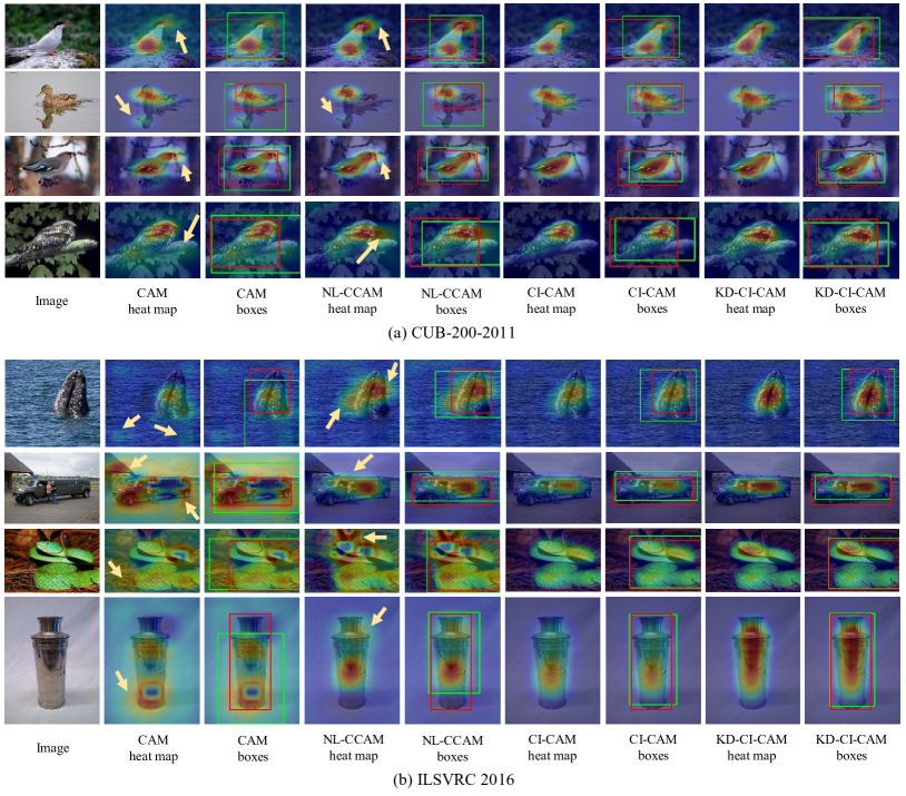
Figure 6: Qualitative object localization results compared with the CAM and NL-CCAM methods. The predicted bounding boxes are in green, and the ground-truth boxes are in red. The yellow arrows indicate the regions suffer from entangled contexts.

4.4 Ablation Study

We conduct two groups of ablation experiments on the CUB-200-2011 wah2011caltech and ILSVRC 2016 russakovsky2015imagenet datasets. The first one is the importance of each module in the architecture, which is designed to demonstrate the effectiveness of the causal context pool and knowledge distillation in the “entangled context” problem and “C-L dilemma” as shown in Table 3 and Figure 1. The other one is the importance of diverse knowledge in the multi-teacher causal distillation framework, which is reported in Table 4.

Importance of each module in the architecture. Our proposed architecture has two components: causal context pool and knowledge distillation. 1) Causal Context Pool. To validate the importance of the causal context pool, we implement our approach with different backbones on the CUB-200-2011 dataset wah2011caltech and ILSVRC 2016 dataset russakovsky2015imagenet . In Table 3, causal context pool significantly brings $11.1\%$, $12.9\%$ and $13.6\%$ improvement in the Top-1 localization, Top-5 localization, and GT-known localization when the backbone is InceptionV3 szegedy2016rethinking on the CUB-200-2011 dataset. Meanwhile, if the backbone is VGG16 simonyan2014very , the causal context pool also brings comprehensive improvement in the Top-1 localization, Top-5 localization, and GT-known localization on both CUB-200-2011 wah2011caltech and ILSVRC 2016 russakovsky2015imagenet datasets. 2) Knowledge Distillation. Employing knowledge distillation can comprehensively improve classification and localization accuracy at all backbones and datasets. For example, knowledge distillation respectively brings extra $4.1\%$, $6.5\%$, and $3.5\%$ improvement in the Top-1 classification, Top-1 localization, and GT-known localization accuracy when the backbone is VGG16 simonyan2014very on the CUB-200-2011 dataset as shown in Table 3. We are surprised to find that knowledge distillation also performs well on the ILSVRC 2016 dataset that it brings extra $0.4\%$, $2.2\%$, and $2.7\%$ improvement in the Top-1 classification, Top-1 localization, and GT-known localization accuracy. 3) Quantitative Analysis. To gain more insights into the effectiveness of the causal context pool and knowledge distillation in the “entangled context” and “C-L dilemma” problems, we plot the visualization results in Figure 1. For example, Figure 1 (a) depicts the effect of causal context pool by comparing different methods. We observe that CI-CAM and KD-CI-CAM employing causal context pool can distinguish the boundary between object and co-occurrence background clearer than vanilla CAM zhou2016learning and NL-CCAM yang2020combinational . Besides, Figure 1 (b) provides multiple independent experiments using different training hyperparameters of CI-CAM and KD-CI-CAM. We find that KD-CI-CAM with knowledge distillation is capable of simultaneously reaching the highest classification and localization accuracy on both VGG16 simonyan2014very and InceptionV3 szegedy2016rethinking .

Importance of diverse knowledge in distillation. To reveal the importance of diverse knowledge in distillation, we set up multiple distillation experiments by using different teachers, which are reported in Table 4. We observe that employing a classification teacher can bring comprehensive improvement in classification performance at all backbones and datasets. And using a localization teacher also comprehensively improves localization performance. Compared with only using a single classification teacher or localization teacher, employing both classification and localization teachers together in distillation can bring larger improvement in both classification and localization performance. Taking VGG16 simonyan2014very as the backbone for example, on the CUB-200-2011 dataset, we obtain $2.3\%$ and $0.9\%$ improvement in the Top-1 classification and Top-5 classification accuracy by only using the classification teacher. When only using the localization teacher, it brings $5.3\%$, $4.2\%$, and $3.4\%$ improvement in the Top-1 localization, Top-5 localization, and GT-known localization. If we use both classification and localization teachers together, our method respectively further improves the performance and brings $4.1\%$, $6.5\%$, and $3.4\%$ improvement in the Top-1 classification, Top-1 localization, and GT-known localization. On the ILSVRC 2016 dataset, we obtain $0.1\%$ and $0.1\%$ improvement in the Top-1 classification and Top-5 classification by only using the classification teacher, respectively. When only using the localization teacher, we respectively obtain $0.9\%$, $1.7\%$, and $2.1\%$ improvement in the Top-1 localization, Top-5 localization, and GT-known localization. Employing both classification and localization teachers together can comprehensively improve the classification and localization performance more than only using a single classification teacher or localization teacher.

4.5 Discussion

In this section, we will discuss how to select our localization teachers according to their Top-1 localization and GT-known localization performance. We conduct three groups of experiments with different backbones on the CUB-200-2011 dataset and ILSVRC 2016 dataset. In Table 5, there are one classification teacher and two kinds of localization teachers in every group experiment. The first localization teacher has the highest Top-1 localization accuracy, and the second one has the highest GT-known localization accuracy.

Taking the CUB-200-2011 dataset for example, we train KD-CI-CAM twice using the same classification teacher and two different localization teachers. If the backbone is VGG16, we first train the first-row KD-CI-CAM using a classification teacher and the first-row localization teacher with higher Top-1 localization accuracy. Then, we train the second-row KD-CI-CAM using the same classification teacher and the second-row localization teacher with higher GT-known localization accuracy. From Table 5, we find that despite the Top-1 classification and Top-1 localization of the second-row localization teacher being significantly lower than that of the first-row localization teacher, the second-row KD-CI-CAM significantly outperforms the first-row KD-CI-CAM under all the evaluation metrics. To validate the generality of this phenomenon, we set up two repeated experiments on the ILSVRC 2016 dataset and InceptionV3 szegedy2016rethinking backbone. Similar to the above observation, KD-CI-CAM can achieve higher accuracy by using the localization teacher with higher GT-known localization performance. As a consequence, we advocate that the selection of localization teacher should be based on its GT-known localization performance rather than the Top-1 localization performance.

5 Conclusions

In this paper, we target the “entangled context” and “C-L dilemma” problems in the WSOL task, which remain unnoticed and unexplored by existing efforts. To this end, we propose a principled framework for solving both “entangled context” and “C-L dilemma” problems in one go. Concretely, we first address the “entangled context” via causal intervention by analyzing the causal relationship between image features, context, and image labels, and cutting off the effect from confounder context to image features. In terms of the model network, we propose a causal context pool to accumulate all contexts of each class, and then re-project the fused contexts to the feature maps of convolutional layers to make the feature boundary clearer. Second, we design a multi-teacher casual distillation framework as shown in Figure 4 (a) for solving the “C-L dilemma” problem by balancing the absorption of classification knowledge and localization knowledge during model training. To our knowledge, we have made a very early attempt to apprehend and approach the “entangled context” and “C-L dilemma” problems for WSOL. Extensive experiments have demonstrated that the “entangled context” and “C-L dilemma” are practical issues within the WSOL task and our proposed methods are effective towards them as shown in Figure 1 and Figure 6.

6 Acknowledge

This work was supported by the National Key Research & Development Project of China (2021ZD0110700), Zhejiang Innovation Foundation (2019R52002), the National Natural Science Foundation of China (U19B2043, 61976185), China Postdoctoral Science Foundation (2022T150567), and the Fundamental Research Funds for the Central Universities.

References

- [1] H Alaskar, A Hussain, B Almaslukh, T Vaiyapuri, Z Sbai, and Arun Kumar Dubey. Deep learning approaches for automatic localization in medical images. Computational Intelligence and Neuroscience, 2022, 2022.
- [2] Sadbhavana Babar and Sukhendu Das. Where to look?: Mining complementary image regions for weakly supervised object localization. In Proceedings of the IEEE/CVF Winter Conference on Applications of Computer Vision, pages 1010–1019, 2021.
- [3] Wonho Bae, Junhyug Noh, and Gunhee Kim. Rethinking class activation mapping for weakly supervised object localization. In European Conference on Computer Vision, pages 618–634. Springer, 2020.
- [4] Aseem Behl, Omid Hosseini Jafari, Siva Karthik Mustikovela, Hassan Abu Alhaija, Carsten Rother, and Andreas Geiger. Bounding boxes, segmentations and object coordinates: How important is recognition for 3d scene flow estimation in autonomous driving scenarios? In Proceedings of the IEEE/CVF International Conference on Computer Vision, 2017.
- [5] Martin Bergtholdt, Jörg Kappes, Stefan Schmidt, and Christoph Schnörr. A study of parts-based object class detection using complete graphs. International journal of computer vision, 87(1):93–117, 2010.
- [6] Lyndon Chan, Mahdi S Hosseini, and Konstantinos N Plataniotis. A comprehensive analysis of weakly-supervised semantic segmentation in different image domains. International Journal of Computer Vision, 129(2):361–384, 2021.
- [7] Defang Chen, Jian-Ping Mei, Can Wang, Yan Feng, and Chun Chen. Online knowledge distillation with diverse peers. In Proceedings of the AAAI Conference on Artificial Intelligence, volume 34, pages 3430–3437, 2020.
- [8] Junsuk Choe and Hyunjung Shim. Attention-based dropout layer for weakly supervised object localization. In Proceedings of the IEEE Conference on Computer Vision and Pattern Recognition, pages 2219–2228, 2019.
- [9] Sandipan Choudhuri, Nibaran Das, Ritesh Sarkhel, and Mita Nasipuri. Object localization on natural scenes: A survey. International Journal of Pattern Recognition and Artificial Intelligence, 32(02):1855001, 2018.
- [10] Ali Diba, Vivek Sharma, Ali Pazandeh, Hamed Pirsiavash, and Luc Van Gool. Weakly supervised cascaded convolutional networks. In Proceedings of the IEEE conference on computer vision and pattern recognition, pages 914–922, 2017.
- [11] Vanessa Didelez and Iris Pigeot. Judea pearl: Causality: Models, reasoning, and inference. Politische Vierteljahresschrift, 42(2):313–315, 2001.
- [12] Mark Everingham, Luc Van Gool, Christopher KI Williams, John Winn, and Andrew Zisserman. The pascal visual object classes (voc) challenge. IJCV, 2010.
- [13] Mengya Gao, Yujun Wang, and Liang Wan. Residual error based knowledge distillation. Neurocomputing, 433:154–161, 2021.
- [14] Yan Gao, Boxiao Liu, Nan Guo, Xiaochun Ye, Fang Wan, Haihang You, and Dongrui Fan. C-midn: Coupled multiple instance detection network with segmentation guidance for weakly supervised object detection. In ICCV, 2019.
- [15] Jianping Gou, Baosheng Yu, Stephen J Maybank, and Dacheng Tao. Knowledge distillation: A survey. International Journal of Computer Vision, 129(6):1789–1819, 2021.
- [16] Guangyu Guo, Junwei Han, Fang Wan, and Dingwen Zhang. Strengthen learning tolerance for weakly supervised object localization. In Proceedings of the IEEE/CVF Conference on Computer Vision and Pattern Recognition, pages 7403–7412, 2021.
- [17] Kaiming He, Xiangyu Zhang, Shaoqing Ren, and Jian Sun. Deep residual learning for image recognition. In CVPR, 2016.
- [18] Byeongho Heo, Minsik Lee, Sangdoo Yun, and Jin Young Choi. Knowledge distillation with adversarial samples supporting decision boundary. In Proceedings of the AAAI conference on artificial intelligence, 2019.
- [19] Geoffrey Hinton, Oriol Vinyals, Jeff Dean, et al. Distilling the knowledge in a neural network. arXiv preprint arXiv:1503.02531, 2(7), 2015.
- [20] Zehao Huang and Naiyan Wang. Like what you like: Knowledge distill via neuron selectivity transfer. arXiv preprint arXiv:1707.01219, 2017.
- [21] Dahun Kim, Donghyeon Cho, Donggeun Yoo, and In So Kweon. Two-phase learning for weakly supervised object localization. In Proceedings of the IEEE International Conference on Computer Vision, pages 3534–3543, 2017.
- [22] Eunji Kim, Siwon Kim, Jungbeom Lee, Hyunwoo Kim, and Sungroh Yoon. Bridging the gap between classification and localization for weakly supervised object localization. In Proceedings of the IEEE/CVF Conference on Computer Vision and Pattern Recognition, pages 14258–14267, 2022.
- [23] Diederik P Kingma and Jimmy Ba. Adam: A method for stochastic optimization. arXiv preprint arXiv:1412.6980, 2014.
- [24] Xu Lan, Xiatian Zhu, and Shaogang Gong. Self-referenced deep learning. In Asian conference on computer vision, pages 284–300. Springer, 2018.
- [25] Li Liu, Wanli Ouyang, Xiaogang Wang, Paul Fieguth, Jie Chen, Xinwang Liu, and Matti Pietikäinen. Deep learning for generic object detection: A survey. International journal of computer vision, 128(2):261–318, 2020.
- [26] Weizeng Lu, Xi Jia, Weicheng Xie, Linlin Shen, Yicong Zhou, and Jinming Duan. Geometry constrained weakly supervised object localization. In European Conference on Computer Vision, pages 481–496. Springer, 2020.
- [27] Yawei Luo, Ping Liu, Tao Guan, Junqing Yu, and Yi Yang. Adversarial style mining for one-shot unsupervised domain adaptation. In Advances in Neural Information Processing Systems, pages 20612–20623, 2020.
- [28] Yawei Luo, Ping Liu, Liang Zheng, Tao Guan, Junqing Yu, and Yi Yang. Category-level adversarial adaptation for semantic segmentation using purified features. IEEE Transactions on Pattern Analysis & Machine Intelligence (TPAMI), 2021.
- [29] Yawei Luo, Liang Zheng, Tao Guan, Junqing Yu, and Yi Yang. Taking a closer look at domain shift: Category-level adversaries for semantics consistent domain adaptation. In Proceedings of the IEEE/CVF Conference on Computer Vision and Pattern Recognition, pages 2507–2516, 2019.
- [30] Yawei Luo, Zhedong Zheng, Liang Zheng, Tao Guan, Junqing Yu, and Yi Yang. Macro-micro adversarial network for human parsing. In Proceedings of the European conference on computer vision (ECCV), pages 418–434, 2018.
- [31] Jinjie Mai, Meng Yang, and Wenfeng Luo. Erasing integrated learning: A simple yet effective approach for weakly supervised object localization. In CVPR, 2020.
- [32] Meng Meng, Tianzhu Zhang, Qi Tian, Yongdong Zhang, and Feng Wu. Foreground activation maps for weakly supervised object localization. In Proceedings of the IEEE/CVF International Conference on Computer Vision, pages 3385–3395, 2021.
- [33] Meng Meng, Tianzhu Zhang, Wenfei Yang, Jian Zhao, Yongdong Zhang, and Feng Wu. Diverse complementary part mining for weakly supervised object localization. IEEE Transactions on Image Processing, 31:1774–1788, 2022.
- [34] Seyed Iman Mirzadeh, Mehrdad Farajtabar, Ang Li, Nir Levine, Akihiro Matsukawa, and Hassan Ghasemzadeh. Improved knowledge distillation via teacher assistant. In Proceedings of the AAAI conference on artificial intelligence, volume 34, pages 5191–5198, 2020.
- [35] Xingjia Pan, Yingguo Gao, Zhiwen Lin, Fan Tang, Weiming Dong, Haolei Yuan, Feiyue Huang, and Changsheng Xu. Unveiling the potential of structure preserving for weakly supervised object localization. In Proceedings of the IEEE/CVF Conference on Computer Vision and Pattern Recognition, pages 11642–11651, 2021.
- [36] Judea Pearl, Madelyn Glymour, and Nicholas P Jewell. Causal inference in statistics: A primer. John Wiley & Sons, 2016.
- [37] Heike Ruppertshofen, Cristian Lorenz, Georg Rose, and Hauke Schramm. Discriminative generalized hough transform for object localization in medical images. International journal of computer assisted radiology and surgery, 8(4):593–606, 2013.
- [38] Olga Russakovsky, Jia Deng, Hao Su, Jonathan Krause, Sanjeev Satheesh, Sean Ma, Zhiheng Huang, Andrej Karpathy, Aditya Khosla, Michael Bernstein, et al. Imagenet large scale visual recognition challenge. IJCV, 2015.
- [39] Henry Schneiderman and Takeo Kanade. Object detection using the statistics of parts. International Journal of Computer Vision, 56(3):151–177, 2004.
- [40] Ramprasaath R Selvaraju, Michael Cogswell, Abhishek Das, Ramakrishna Vedantam, Devi Parikh, and Dhruv Batra. Grad-cam: Visual explanations from deep networks via gradient-based localization. In ICCV, 2017.
- [41] Feifei Shao, Long Chen, Jian Shao, Wei Ji, Shaoning Xiao, Lu Ye, Yueting Zhuang, and Jun Xiao. Deep learning for weakly-supervised object detection and localization: A survey. Neurocomputing, 2022.
- [42] Feifei Shao, Yawei Luo, Ping Liu, Jie Chen, Yi Yang, Yulei Lu, and Jun Xiao. Active learning for point cloud semantic segmentation via spatial-structural diversity reasoning. arXiv preprint arXiv:2202.12588, 2022.
- [43] Feifei Shao, Yawei Luo, Li Zhang, Lu Ye, Siliang Tang, Yi Yang, and Jun Xiao. Improving weakly supervised object localization via causal intervention. In Proceedings of the 29th ACM International Conference on Multimedia, pages 3321–3329, 2021.
- [44] Arvind Kumar Shekar, Liang Gou, Liu Ren, and Axel Wendt. Label-free robustness estimation of object detection cnns for autonomous driving applications. International Journal of Computer Vision, 129(4):1185–1201, 2021.
- [45] Karen Simonyan and Andrew Zisserman. Very deep convolutional networks for large-scale image recognition. In arXiv, 2014.
- [46] Lingyun Song, Jun Liu, Mingxuan Sun, and Xuequn Shang. Weakly supervised group mask network for object detection. International Journal of Computer Vision, 129(3):681–702, 2021.
- [47] Christian Szegedy, Wei Liu, Yangqing Jia, Pierre Sermanet, Scott Reed, Dragomir Anguelov, Dumitru Erhan, Vincent Vanhoucke, and Andrew Rabinovich. Going deeper with convolutions. In CVPR, 2015.
- [48] Christian Szegedy, Vincent Vanhoucke, Sergey Ioffe, Jon Shlens, and Zbigniew Wojna. Rethinking the inception architecture for computer vision. In Proceedings of the IEEE conference on computer vision and pattern recognition, pages 2818–2826, 2016.
- [49] Kaihua Tang, Jianqiang Huang, and Hanwang Zhang. Long-tailed classification by keeping the good and removing the bad momentum causal effect. arXiv preprint arXiv:2009.12991, 2020.
- [50] Jonathan Tompson, Ross Goroshin, Arjun Jain, Yann LeCun, and Christoph Bregler. Efficient object localization using convolutional networks. In Proceedings of the IEEE conference on computer vision and pattern recognition, pages 648–656, 2015.
- [51] Catherine Wah, Steve Branson, Peter Welinder, Pietro Perona, and Serge Belongie. The caltech-ucsd birds-200-2011 dataset. 2011.
- [52] Jun Wei, Qin Wang, Zhen Li, Sheng Wang, S Kevin Zhou, and Shuguang Cui. Shallow feature matters for weakly supervised object localization. In Proceedings of the IEEE/CVF Conference on Computer Vision and Pattern Recognition, pages 5993–6001, 2021.
- [53] Yunchao Wei, Zhiqiang Shen, Bowen Cheng, Honghui Shi, Jinjun Xiong, Jiashi Feng, and Thomas Huang. Ts2c: Tight box mining with surrounding segmentation context for weakly supervised object detection. In Proceedings of the European Conference on Computer Vision (ECCV), pages 434–450, 2018.
- [54] Peter Welinder, Steve Branson, Takeshi Mita, Catherine Wah, Florian Schroff, Serge Belongie, and Pietro Perona. Caltech-ucsd birds 200. 2010.
- [55] Guile Wu and Shaogang Gong. Peer collaborative learning for online knowledge distillation. In Proceedings of the AAAI Conference on Artificial Intelligence, volume 35, pages 10302–10310, 2021.
- [56] Pingyu Wu, Wei Zhai, and Yang Cao. Background activation suppression for weakly supervised object localization. In 2022 IEEE/CVF Conference on Computer Vision and Pattern Recognition (CVPR), pages 14228–14237. IEEE, 2022.
- [57] Xiang Wu, Ran He, Yibo Hu, and Zhenan Sun. Learning an evolutionary embedding via massive knowledge distillation. International Journal of Computer Vision, 128(8):2089–2106, 2020.
- [58] Jinheng Xie, Cheng Luo, Xiangping Zhu, Ziqi Jin, Weizeng Lu, and Linlin Shen. Online refinement of low-level feature based activation map for weakly supervised object localization. In Proceedings of the IEEE/CVF International Conference on Computer Vision, pages 132–141, 2021.
- [59] Jilan Xu, Junlin Hou, Yuejie Zhang, Rui Feng, Rui-Wei Zhao, Tao Zhang, Xuequan Lu, and Shang Gao. Cream: Weakly supervised object localization via class re-activation mapping. In Proceedings of the IEEE/CVF Conference on Computer Vision and Pattern Recognition, pages 9437–9446, 2022.
- [60] Kelvin Xu, Jimmy Ba, Ryan Kiros, Kyunghyun Cho, Aaron Courville, Ruslan Salakhudinov, Rich Zemel, and Yoshua Bengio. Show, attend and tell: Neural image caption generation with visual attention. In International conference on machine learning, pages 2048–2057. PMLR, 2015.
- [61] Haolan Xue, Chang Liu, Fang Wan, Jianbin Jiao, Xiangyang Ji, and Qixiang Ye. Danet: Divergent activation for weakly supervised object localization. In ICCV, 2019.
- [62] Seunghan Yang, Yoonhyung Kim, Youngeun Kim, and Changick Kim. Combinational class activation maps for weakly supervised object localization. In WACV, 2020.
- [63] Zhongqi Yue, Hanwang Zhang, Qianru Sun, and Xian-Sheng Hua. Interventional few-shot learning. arXiv preprint arXiv:2009.13000, 2020.
- [64] Sukmin Yun, Jongjin Park, Kimin Lee, and Jinwoo Shin. Regularizing class-wise predictions via self-knowledge distillation. In Proceedings of the IEEE/CVF conference on computer vision and pattern recognition, pages 13876–13885, 2020.
- [65] Chen-Lin Zhang, Yun-Hao Cao, and Jianxin Wu. Rethinking the route towards weakly supervised object localization. In Proceedings of the IEEE/CVF Conference on Computer Vision and Pattern Recognition, pages 13460–13469, 2020.
- [66] Dong Zhang, Hanwang Zhang, Jinhui Tang, Xiansheng Hua, and Qianru Sun. Causal intervention for weakly-supervised semantic segmentation. arXiv preprint arXiv:2009.12547, 2020.
- [67] Xiaolin Zhang, Yunchao Wei, Jiashi Feng, Yi Yang, and Thomas S Huang. Adversarial complementary learning for weakly supervised object localization. In Proceedings of the IEEE Conference on Computer Vision and Pattern Recognition, pages 1325–1334, 2018.
- [68] Xiaolin Zhang, Yunchao Wei, Guoliang Kang, Yi Yang, and Thomas Huang. Self-produced guidance for weakly-supervised object localization. In Proceedings of the European conference on computer vision (ECCV), pages 597–613, 2018.
- [69] Xiaolin Zhang, Yunchao Wei, and Yi Yang. Inter-image communication for weakly supervised localization. In European Conference on Computer Vision, pages 271–287. Springer, 2020.
- [70] Tao Zhao, Junwei Han, Le Yang, Binglu Wang, and Dingwen Zhang. Soda: Weakly supervised temporal action localization based on astute background response and self-distillation learning. International Journal of Computer Vision, 129(8):2474–2498, 2021.
- [71] Zhaohui Zheng, Rongguang Ye, Qibin Hou, Dongwei Ren, Ping Wang, Wangmeng Zuo, and Ming-Ming Cheng. Localization distillation for object detection. arXiv preprint arXiv:2204.05957, 2022.
- [72] Bolei Zhou, Aditya Khosla, Agata Lapedriza, Aude Oliva, and Antonio Torralba. Learning deep features for discriminative localization. In CVPR, 2016.