Generalised (non-singular) entropy functions with applications to cosmology and black holes

Abstract

The growing interest of different entropy functions proposed so far (like the Bekenstein-Hawking, Tsallis, Rényi, Barrow, Sharma-Mittal, Kaniadakis and Loop Quantum Gravity entropies) towards black hole thermodynamics as well as towards cosmology lead to the natural question that whether there exists a generalized entropy function that can generalize all these known entropies. With this spirit, we propose a new 4-parameter entropy function that seems to converge to the aforementioned known entropies for certain limits of the entropic parameters. The proposal of generalized entropy is extended to non-singular case, in which case , the entropy proves to be singular-free during the entire cosmological evolution of the universe. The hallmark of such generalized entropies is that it helps us to fundamentally understand one of the important physical quantities namely “entropy”. Consequently we address the implications of the generalized entropies on black hole thermodynamics as well as on cosmology, and discuss various constraints of the entropic parameters from different perspectives.

I Introduction

One of the most important discoveries in theoretical physics is the black body radiation of a black hole, which is described by a certain temperature and by a Bekenstein-Hawking entropy function Bekenstein:1973ur ; Hawking:1975vcx (see Bardeen:1973gs ; Wald:1999vt for extensive reviews). On contrary to classical thermodynamics where the entropy is proportional to volume of the system under consideration, the Bekenstein-Hawking entropy is proportional to the area of the black hole horizon. Such unusual behaviour of the black hole entropy leads to the proposals of different entropy functions, such as, the Tsallis Tsallis:1987eu , Rényi Renyi , Barrow Barrow:2020tzx , Sharma-Mittal SayahianJahromi:2018irq , Kaniadakis Kaniadakis:2005zk and the Loop Quantum Gravity entropies Majhi:2017zao are well known entropy functions proposed so far. All of these known entropies have the common properties like – (1) they seem to be the monotonic increasing function with respect to the Bekenstein-Hawkinh entropy variable, (2) they obey the third law of thermodynamics, in particular, all of these entropies tend to zero as $S\rightarrow 0$ (where $S$ represents the Bekenstein-Hawking entropy) and (3) they converge to the Bekenstein-Hawking entropy for suitable choices of the respective entropic parameter, for example, the Tsallis entropy goes to the Bekenstein-Hawking entropy when the Tsallis exponent tends to unity. Furthermore, these entropies have rich consequences towards cosmology, particularly in describing the dark energy era of the universe Li:2004rb ; Li:2011sd ; Wang:2016och ; Pavon:2005yx ; Nojiri:2005pu ; Landim:2022jgr ; Zhang:2005yz ; Guberina:2005fb ; Elizalde:2005ju ; Ito:2004qi ; Gong:2004cb ; BouhmadiLopez:2011xi ; Malekjani:2012bw ; Khurshudyan:2016gmb ; Landim:2015hqa ; Gao:2007ep ; Li:2008zq ; Anagnostopoulos:2020ctz ; Zhang:2005hs ; Li:2009bn ; Feng:2007wn ; Zhang:2009un ; Lu:2009iv ; Micheletti:2009jy ; Mukherjee:2017oom ; Nojiri:2017opc ; Nojiri:2019skr ; Saridakis:2020zol ; Barrow:2020kug ; Adhikary:2021xym ; Srivastava:2020cyk ; Bhardwaj:2021chg ; Chakraborty:2020jsq ; Sarkar:2021izd . The growing interest of such known entropies and due to their common properties lead to a natural question that whether there exists some generalized entropy function which is able to generalize all the known entropies proposed so far for suitable limits of the parameters.

The entropy functions are extensively applied in the realm of black hole thermodynamics and cosmological evolution of the universe. Recently we showed that the entropic cosmology corresponding to different entropy functions can be equivalently represented by holographic cosmology where the equivalent holographic cut-offs come in terms of either particle horizon and its derivative or the future horizon and its derivative. One of the mysteries in today’s cosmology is to explain the acceleration of the universe in the high as well as in the low curvature regime, known as inflation and the dark energy era respectively. These eras are well described by entropic cosmology or equivalently by holographic cosmology Li:2004rb ; Li:2011sd ; Wang:2016och ; Pavon:2005yx ; Nojiri:2005pu ; Landim:2022jgr ; Zhang:2005yz ; Guberina:2005fb ; Elizalde:2005ju ; Ito:2004qi ; Gong:2004cb ; BouhmadiLopez:2011xi ; Malekjani:2012bw ; Khurshudyan:2016gmb ; Landim:2015hqa ; Gao:2007ep ; Li:2008zq ; Anagnostopoulos:2020ctz ; Zhang:2005hs ; Li:2009bn ; Feng:2007wn ; Zhang:2009un ; Lu:2009iv ; Micheletti:2009jy ; Mukherjee:2017oom ; Nojiri:2017opc ; Nojiri:2019skr ; Saridakis:2020zol ; Barrow:2020kug ; Adhikary:2021xym ; Srivastava:2020cyk ; Bhardwaj:2021chg ; Chakraborty:2020jsq ; Sarkar:2021izd ; Nojiri:2022aof ; Nojiri:2022dkr ; Horvat:2011wr ; Nojiri:2019kkp ; Paul:2019hys ; Bargach:2019pst ; Elizalde:2019jmh ; Oliveros:2019rnq ; Mohammadi:2022vru ; Chakraborty:2020tge , and more interestingly, the entropic cosmology proves to be useful to unify the early inflation and the late dark energy era of the universe in a covariant manner Nojiri:2020wmh . Apart from the inflation, the holographic cosmology turns out to be useful in describing the bouncing scenario Nojiri:2019yzg ; Brevik:2019mah . In regard to the bounce scenario, the energy density sourced from the holographic principle or from some entropy function under consideration helps to violate the null energy condition at a finite time, which in turn triggers a non-singular bouncing universe. However here it deserves mentioning that all the known entropies mentioned above (like Tsallis , Rényi, Barrow, Sharma-Mittal, Kaniadakis and the Loop Quantum Gravity entropies) become singular (or diverge) at a certain cosmological evolution of the universe, particularly in the context of bounce cosmology. Actually such entropies contain a factor that is proportional to $1/H^{2}$ (where $H$ is the Hubble parameter), and thus they diverge at the instant when the Hubble parameter vanishes, i.e, at the instant of a bounce in bouncing cosmology. This makes such known entropies ill-defined in describing a non-singular bounce scenario.

Based on the above arguments, the questions that naturally arise are following:

• Does there exist a generalized entropy function that generalizes all the known entropies proposed so far ?

• If so, then what is its implications on black hole thermodynamics as well as on cosmology ?

• Similar to the known entropies, is the generalized entropy becomes singular at the instant when the Hubble parameter of the universe vanishes, for instance, in the bounce cosmology ? If so, then does there exist an entropy function that generalizes all the known entropies, and at the same time, also proves to be singular-free during the entire cosmic evolution of the universe ?

The present article, based on some of our previous works Nojiri:2022aof ; Nojiri:2022dkr ; OP-submitted , gives a brief review in answering the above questions. The notations or conventions in this article are following: we will follow the $\left(-,+,+,+\right)$ signature of the spacetime metric, and $\kappa^{2}=8\pi G=\frac{1}{M_{\mathrm{Pl}}^{2}}$ where $G$ is the Newton’s constant or $M_{\mathrm{Pl}}$ denotes the four dimensional Planck mass. In regard to the cosmological evolution, $a(t)$ and $H(t)$ are the scale factor and the Hubble parameter of the universe respectively, $N$ being the e-folding number, an overprime will denote $\frac{d}{d\eta}$ where $\eta$ is the conformal time, an overdot will symbolize $\frac{d}{dt}$ with $t$ being the cosmic time, otherwise an overprime with some argument will represent the derivative of the function with respect to that argument.

II Possible generalizations of known entropies

Here we will propose a generalized four-parameter entropy function which can lead to various known entropy functions proposed so far for suitable choices of the parameters.

Let us start with the Bekenstein-Hawking entropy, the very first proposal of thermodynamical entropy of black hole physics Bekenstein:1973ur ; Hawking:1975vcx ,

$$S=\frac{A}{4G}\,,$$ (1)

where $A=4\pi r_{h}^{2}$ is the area of the horizon and $r_{h}$ is the horizon radius. Consequently, different entropy functions have been introduced depending on the system under consideration. Let us briefly recall some of the entropy functions proposed so far:

• For the systems with long range interactions where the Boltzmann-Gibbs entropy is not applied, one needs to introduce the Tsallis entropy which is given by Tsallis:1987eu ,

  $$S_{T}=\frac{A_{0}}{4G}\left(\frac{A}{A_{0}}\right)^{\delta}\,,$$ (2)

  where $A_{0}$ is a constant and $\delta$ is the exponent.

• The Rényi entropy is given by Renyi ,

  $$S_{\mathrm{R}}=\frac{1}{\alpha}\ln\left(1+\alpha S\right)\,,$$ (3)

  where $S$ is identified with the Bekenstein-Hawking entropy and $\alpha$ is a parameter.

• The Barrow entropy is given by Barrow:2020tzx ,

  $$S_{\mathrm{B}}=\left(\frac{A}{A_{\mathrm{Pl}}}\right)^{1+\Delta/2}\,,$$ (4)

  where $A$ is the usual black hole horizon area and $A_{\mathrm{Pl}}=4G$ is the Planck area. The Barrow entropy describes the fractal structures of black hole that may generate from quantum gravity effects.

• The Sharma-Mittal entropy is given by SayahianJahromi:2018irq ,

  $$S_{SM}=\frac{1}{R}\left[\left(1+\delta~{}S\right)^{R/\delta}-1\right]\,,$$ (5)

  where $R$ and $\delta$ are two parameters. The Sharma-Mittal entropy can be regarded as a possible combination of the Tsallis and Rényi entropies.

• The Kaniadakis entropy function is of the following form Kaniadakis:2005zk :

  $$S_{K}=\frac{1}{K}\sinh{\left(KS\right)}\,,$$ (6)

  where $K$ is a phenomenological parameter.

• In the context of Loop Quantum Gravity, one may get the following entropy function Majhi:2017zao :

  $$S_{q}=\frac{1}{\left(1-q\right)}\left[\mathrm{e}^{(1-q)\Lambda(\gamma_{0})S}-1\right]\,,$$ (7)

  where $q$ is the exponent and $\Lambda(\gamma_{0})=\ln{2}/\left(\sqrt{3}\pi\gamma_{0}\right)$ with $\gamma_{0}$ being the Barbero-Immirzi parameter. The $\gamma_{0}$ generally takes either $\gamma_{0}=\frac{\ln{2}}{\pi\sqrt{3}}$ or $\gamma_{0}=\frac{\ln{3}}{2\pi\sqrt{2}}$. However with $\gamma_{0}=\frac{\ln{2}}{\pi\sqrt{3}}$, $\Lambda(\gamma_{0})$ becomes unity and $S_{q}$ resembles with the Bekenstein-Hawking entropy for $q\rightarrow 1$.

All the above entropies – (1) obeys the generalized third law of thermodynamics, i.e the entropy function(s) vanishes at the limit $S\rightarrow 0$; (2) monotonically increases with respect to the Bekenstein-Hawking variable and (3) converges to the Bekenstein-Hawking entropy for suitable limit of the entropic parameter, for example, the Tsallis entropy tends to $S$ at $\delta=1$.

In Nojiri:2022aof ; Nojiri:2022dkr , we proposed two different entropy functions containing 6-parameters and 4-parameters respectively, which can generalize all the known entropies mentioned from Eq.(2) to Eq.(7). In particular, the generalized entropies are given by,

$$\mathrm{6~{}parameter~{}entropy:}~{}~{}~{}~{}~{}\mathcal{S}_{\mathrm{6}}\left[\alpha_{\pm},\beta_{\pm},\gamma_{\pm}\right] = \frac{1}{\alpha_{+}+\alpha_{-}}\left[\left(1+\frac{\alpha_{+}}{\beta_{+}}\,\mathcal{S}^{\gamma_{+}}\right)^{\beta_{+}}-\left(1+\frac{\alpha_{-}}{\beta_{-}}\,\mathcal{S}^{\gamma_{-}}\right)^{-\beta_{-}}\right]\,,$$ (8)

$$\mathrm{4~{}parameter~{}entropy:}~{}~{}~{}~{}~{}S_{\mathrm{g}}\left[\alpha_{+},\alpha_{-},\beta,\gamma\right] = \frac{1}{\gamma}\left[\left(1+\frac{\alpha_{+}}{\beta}~{}S\right)^{\beta}-\left(1+\frac{\alpha_{-}}{\beta}~{}S\right)^{-\beta}\right]\,,$$ (9)

where the respective parameters are given in the argument and they are assumed to be positive. Here $S$ is the Bekenstein-Hawking entropy. Below we prove the generality of the above generalized entropy functions, in particular, we show that both the generalized entropies reduce to the known entropies mentioned in Eqs. (2), (3), (4), (5), (6), and (7) for suitable choices of the respective parameters. Here we establish it particularly for the 4-parameter entropy function, while the similar calculations hold for the 6-parameter entropy as well Nojiri:2022aof .

• For $\alpha_{+}\rightarrow\infty$ and $\alpha_{-}=0$, one gets

  $$S_{\mathrm{g}}=\frac{1}{\gamma}\left(\frac{\alpha_{+}}{\beta}\right)^{\beta}S^{\beta}\,.$$

  If we further choose $\gamma=\left(\alpha_{+}/\beta\right)^{\beta}$, then the generalized entropy reduces to

  $$S_{\mathrm{g}}=S^{\beta}\,.$$

  Therefore with $\beta=\delta$ or $\beta=1+\Delta$, the generalized entropy resembles with the Tsallis entropy or with the Barrow entropy respectively.

• For $\alpha_{-}=0$, $\beta\rightarrow 0$ and $\frac{\alpha_{+}}{\beta}\rightarrow\mathrm{finite}$ – Eq. (9) leads to,

  $$S_{\mathrm{g}}=\frac{1}{\gamma}\left[\left(1+\frac{\alpha_{+}}{\beta}~{}S\right)^{\beta}-1\right]=\frac{1}{\gamma}\left[\exp{\left\{\beta\ln{\left(1+\frac{\alpha_{+}}{\beta}~{}S\right)}\right\}}-1\right]\approx\frac{1}{\left(\gamma/\beta\right)}\ln{\left(1+\frac{\alpha_{+}}{\beta}~{}S\right)}\,.$$

  Further choosing $\gamma=\alpha_{+}$ and identifying $\frac{\alpha_{+}}{\beta}=\alpha$, we can write the above expression as,

  $$S_{\mathrm{g}}=\frac{1}{\alpha}\ln{\left(1+\alpha~{}S\right)}\,,$$ (10)

  i.e., $S_{\mathrm{g}}$ reduces to the Rényi entropy.

• In the case when $\alpha_{-}=0$, the generalized entropy becomes,

  $$S_{\mathrm{g}}=\frac{1}{\gamma}\left[\left(1+\frac{\alpha_{+}}{\beta}~{}S\right)^{\beta}-1\right]\,.$$ (11)

  Thereby identifying $\gamma=R$, $\alpha_{+}=R$ and $\beta=R/\delta$, the generalized entropy function $S_{\mathrm{g}}$ gets similar to the Sharma-Mittal entropy.

• For $\beta\rightarrow\infty$, $\alpha_{+}=\alpha_{-}=\frac{\gamma}{2}=K$, we may write Eq. (9) as,

  $$S_{\mathrm{g}}= \,\frac{1}{2K}\lim_{\beta\rightarrow\infty}\left[\left(1+\frac{K}{\beta}~{}S\right)^{\beta}-\left(1+\frac{K}{\beta}~{}S\right)^{-\beta}\right]$$

  $$= \,\frac{1}{2K}\left[\mathrm{e}^{KS}-\mathrm{e}^{-KS}\right]=\frac{1}{K}\sinh{\left(KS\right)}\rightarrow\mathrm{Kaniadakis~{}entropy}\,.$$ (12)

• Finally, with $\alpha_{-}=0$, $\beta\rightarrow\infty$ and $\gamma=\alpha_{+}=(1-q)$, Eq. (9) immediately yields,

  $$S_{\mathrm{g}}=\frac{1}{(1-q)}\left[\mathrm{e}^{(1-q)S}-1\right]\,,$$

  which is the Loop Quantum Gravity entropy with $\Lambda(\gamma_{0})=1$ or equivalently $\gamma_{0}=\frac{\ln{2}}{\pi\sqrt{3}}$.

Furthermore, the generalized entropy function in Eq. (9) shares the following properties: (1) $S_{\mathrm{g}}\rightarrow 0$ for $S\rightarrow 0$. (2) The entropy $S_{\mathrm{g}}\left[\alpha_{+},\alpha_{-},\beta,\gamma\right]$ is a monotonically increasing function with $S$ because both the terms $\left(1+\frac{\alpha_{+}}{\beta}~{}S\right)^{\beta}$ and $-\left(1+\frac{\alpha_{-}}{\beta}~{}S\right)^{-\beta}$ present in the expression of $S_{\mathrm{g}}$ increase with $S$. (3) $S_{\mathrm{g}}\left[\alpha_{+},\alpha_{-},\beta,\gamma\right]$ seems to converge to the Bekenstein-Hawking entropy at certain limit of the parameters. In particular, for $\alpha_{+}\rightarrow\infty$, $\alpha_{-}=0$, $\gamma=\left(\alpha_{+}/\beta\right)^{\beta}$ and $\beta=1$, the generalized entropy function in Eq. (9) becomes equivalent to the Bekenstein-Hawking entropy.

Here it deserves mentioning that beside the entropy function proposed in Eq. (9) which contains four parameters, one may consider a three parameter entropy having the following form:

$$S_{3}[\alpha,\beta,\gamma]=\frac{1}{\gamma}\left[\left(1+\frac{\alpha}{\beta}~{}S\right)^{\beta}-1\right]\,,$$ (13)

where $\alpha$, $\beta$ and $\gamma$ are the parameters. The above form of $S_{3}[\alpha,\beta,\gamma]$ satisfies all the properties, like – (1) $S_{3}[\alpha,\beta,\gamma]\rightarrow 0$ for $S\rightarrow 0$, (2) $S_{3}$ is an increasing function with $S$ and (3) $S_{3}$ has a Bekenstein-Hawking entropy limit for the choices: $\alpha\rightarrow\infty$, $\gamma=\left(\alpha/\beta\right)^{\beta}$ and $\beta=1$ respectively. However $S_{3}[\alpha,\beta,\gamma]$ is not able to generalize all the known entropies mentioned from Eq. (2) to Eq. (7), in particular, $S_{3}[\alpha,\beta,\gamma]$ does not reduce to the Kaniadakis entropy for any possible choices of the parameters.

Conjecture - I: Based on our findings, we propose the following postulate in regard to the generalized entropy function – “The minimum number of parameters required in a generalized entropy function that can generalize all the known entropies mentioned from Eq. (2) to Eq. (7) is equal to four”.

Below we will address the possible implications of such generalized entropies on black hole thermodynamics as well as on cosmology.

III Black hole thermodynamics with 3-parameter generalized entropy

It is interesting to see what happens when the generalized entropy (13) is ascribed to the prototypical black hole, given by the Schwarzschild geometry Nojiri:2022aof

$$ds^{2}=-f(r)\,dt^{2}+\frac{dr^{2}}{f(r)}+r^{2}d\Omega^{2}_{(2)}\,,\quad\quad f(r)=1-\frac{2GM}{r}\,,$$ (14)

where $M$ is the black hole mass and $d\Omega^{2}_{(2)}=d\vartheta^{2}+\sin^{2}\vartheta\,d\varphi^{2}$ is the line element on the unit two-sphere. The black hole event horizon is located at the Schwarzschild radius

$$r_{\mathrm{H}}=2GM\,.$$ (15)

Studying quantum field theory on the spacetime with this horizon, Hawking discovered that the Schwarzschild black hole radiates with a blackbody spectrum at the temperature

$$T_{\mathrm{H}}=\frac{1}{8\pi GM}\,.$$ (16)

As explained in general below, if we assume that the mass $M$ coincides with the thermodynamical energy, then the temperature obtained from the thermodynamical law is different from the Hawking temperature, a contradiction for observers detecting Hawking radiation. Alternatively, if the Hawking temperature $T_{\mathrm{H}}$ is identified with the physical black hole temperature, the obtained thermodynamical energy differs from the Schwarzschild mass $M$ even for the Tsallis entropy or the Rényi entropy, which seems to imply a breakdown of energy conservation.

If the mass $M$ coincides with the thermodynamical energy $E$ of the system due to energy conservation, as in, in order for this system to be consistent with the thermodynamical equation $d\mathcal{S}_{G}=dE/T$ one needs to define the generalized temperature $T_{\mathrm{G}}$ as

$$\frac{1}{T_{\mathrm{G}}}\equiv\frac{d\mathcal{S}_{\mathrm{G}}}{dM}$$ (17)

which is, in general, different from the Hawking temperature $T_{\mathrm{H}}$. For example, in the case of the entropy (13), one has

$$\frac{1}{T_{\mathrm{G}}}=\frac{\alpha}{\gamma}\left(1+\frac{\alpha}{\beta}\,\mathcal{S}\right)^{\beta-1}\frac{d\mathcal{S}}{dM}=\frac{\alpha}{\gamma}\left(1+\frac{\alpha}{\beta}\,\mathcal{S}\right)^{\beta-1}\frac{1}{T_{\mathrm{H}}}\,,$$ (18)

where

$$\mathcal{S}=\frac{A}{4G}=4\pi GM^{2}=\frac{1}{16\pi G{T_{\mathrm{H}}}^{2}}\,.$$ (19)

Because $\frac{\alpha}{\gamma}\left(1+\,\frac{\alpha}{\beta}\,\mathcal{S}\right)^{\beta-1}\neq 1$, it is necessarily $T_{\mathrm{G}}\neq T_{\mathrm{H}}$. Since the Hawking temperature (16) is the temperature perceived by observers detecting Hawking radiation, the generalized temperature $T_{\mathrm{G}}$ in (18) cannot be a physically meaningful temperature.

In Eq. (17), assuming that the thermodynamical energy $E$ is the black hole mass $M$ leads to an unphysical result. As an alternative, assume that the thermodynamical temperature $T$ coincides with the Hawking temperature $T_{\mathrm{H}}$ instead of assuming $E=M$. This assumption leads to

$$dE_{\mathrm{G}}=T_{\mathrm{H}}\,d\mathcal{S}_{\mathrm{G}}=\frac{d\mathcal{S}_{\mathrm{G}}}{d\mathcal{S}}\,\frac{d\mathcal{S}}{\sqrt{16\pi G\mathcal{S}}}$$ (20)

which, in the case of Eq. (13), yields

$$dE_{\mathrm{G}} = \frac{\alpha}{\gamma}\left(1+\frac{\alpha}{\beta}\,\mathcal{S}\right)^{\beta-1}\,\frac{d\mathcal{S}}{\sqrt{16\pi G\mathcal{S}}}$$ (21)

$$= \frac{\alpha}{\gamma\sqrt{16\pi G}}\left[\mathcal{S}^{-1/2}+\frac{\alpha\left(\beta-1\right)}{\beta}\,\mathcal{S}^{1/2}+\mathcal{O}\left(\mathcal{S}^{3/2}\right)\right]\,.$$

The integration of Eq. (21) gives

$$E_{\mathrm{G}} = \frac{\alpha}{\gamma\sqrt{16\pi G}}\left[2\mathcal{S}^{1/2}+\frac{2\alpha\left(\beta-1\right)}{3\beta}\,\mathcal{S}^{3/2}+\mathcal{O}\left(\mathcal{S}^{5/2}\right)\right]$$ (22)

$$= \frac{\alpha}{\gamma}\left[M+\frac{4\pi G\alpha\left(\beta-1\right)}{3\beta}M^{3}+\mathcal{O}\left(M^{5}\right)\right]\,,$$

where the integration constant is determined by the condition that $E_{\mathrm{G}}=0$ when $M=0$. Even when $\alpha=\gamma$, due to the correction $\frac{4\pi G\alpha\left(\beta-1\right)}{3\beta}M^{3}$, the expression (22) of the thermodynamical energy $E_{\mathrm{R}}$ obtained differs from the black hole mass $M$, $E_{\mathrm{G}}\neq E$, which seems unphysical.

IV Cosmology with the 4-parameter generalized entropy

Here we consider the 4-parameter generalized entropy (9), which is indeed more generalized compared to the 3-parameter entropy function of Eq.(13), to describe the cosmological behaviour of the universe Nojiri:2022dkr . In particular, we examine whether the 4-parameter entropy function results to an unified scenario of early inflation and the late dark energy era of the universe.

The Friedmann-Lemaître-Robertson-Walker space-time with flat spacial part will serve our purpose, in particular,

$$ds^{2}=-dt^{2}+a^{2}(t)\sum_{i=1,2,3}\left(dx^{i}\right)^{2}\,.$$ (23)

Here $a(t)$ is called as a scale factor.

The radius $r_{\mathrm{H}}$ of the cosmological horizon is given by

$$r_{\mathrm{H}}=\frac{1}{H}\,,$$ (24)

with $H=\dot{a}/a$ is the Hubble parameter of the universe. Then the entropy contained within the cosmological horizon can be obtained from the Bekenstein-Hawking relation Padmanabhan:2009vy . Furthermore the flux of the energy $E$, or equivalently, the increase of the heat $Q$ in the region comes as

$$dQ=-dE=-\frac{4\pi}{3}r_{\mathrm{H}}^{3}\dot{\rho}dt=-\frac{4\pi}{3H^{3}}\dot{\rho}~{}dt=\frac{4\pi}{H^{2}}\left(\rho+p\right)~{}dt\,,$$ (25)

where, in the last equality, we use the conservation law: $0=\dot{\rho}+3H\left(\rho+p\right)$. Then from the Hawking temperature Cai:2005ra

$$T=\frac{1}{2\pi r_{\mathrm{H}}}=\frac{H}{2\pi}\,,$$ (26)

and by using the first law of thermodynamics $TdS=dQ$, one obtains $\dot{H}=-4\pi G\left(\rho+p\right)$. Integrating the expression immediately leads to the first FRW equation,

$$H^{2}=\frac{8\pi G}{3}\rho+\frac{\Lambda}{3}\,,$$ (27)

where the integration constant $\Lambda$ can be treated as a cosmological constant.

Instead of the Bekenstein-Hawking entropy of Eq. (1), we may use the generalized entropy in Eq. (9), in regard to which, the first law of thermodynamics leads to the following equation:

$$\dot{H}\left(\frac{\partial S_{\mathrm{g}}}{\partial S}\right)=-4\pi G\left(\rho+p\right)\,.$$ (28)

With the explicit form of $S_{\mathrm{g}}$ from Eq. (9), the above equation turns out to be,

$$\frac{1}{\gamma}\left[\alpha_{+}\left(1+\frac{\pi\alpha_{+}}{\beta GH^{2}}\right)^{\beta-1}+\alpha_{-}\left(1+\frac{\pi\alpha_{-}}{\beta GH^{2}}\right)^{-\beta-1}\right]\dot{H}=-4\pi G\left(\rho+p\right)$$ (29)

where we use $S=A/(4G)=\pi/(GH^{2})$. Using the conservation relation of the matter fields, i.e., $\dot{\rho}+3H\left(\rho+p\right)=0$, Eq. (29) can be written as,

$$\frac{2}{\gamma}\left[\alpha_{+}\left(1+\frac{\pi\alpha_{+}}{\beta GH^{2}}\right)^{\beta-1}+\alpha_{-}\left(1+\frac{\pi\alpha_{-}}{\beta GH^{2}}\right)^{-\beta-1}\right]H~{}dH=\left(\frac{8\pi G}{3}\right)d\rho\,,$$

on integrating which, we obtain,

$$\frac{GH^{4}\beta}{\pi\gamma} \,\left[\frac{1}{\left(2+\beta\right)}\left(\frac{GH^{2}\beta}{\pi\alpha_{-}}\right)^{\beta}~{}2F_{1}\left(1+\beta,2+\beta,3+\beta,-\frac{GH^{2}\beta}{\pi\alpha_{-}}\right)\right.$$

$$\,\left.+\frac{1}{\left(2-\beta\right)}\left(\frac{GH^{2}\beta}{\pi\alpha_{+}}\right)^{-\beta}~{}2F_{1}\left(1-\beta,2-\beta,3-\beta,-\frac{GH^{2}\beta}{\pi\alpha_{+}}\right)\right]=\frac{8\pi G\rho}{3}+\frac{\Lambda}{3}\,,$$ (30)

where $\Lambda$ is the integration constant (known as the cosmological constant) and $2F_{1}(\mathrm{arguments})$ denotes the Hypergeometric function. Eq. (29) and Eq. (30) represent the modified Friedmann equations corresponding to the generalized entropy function $S_{\mathrm{g}}$. In the next section, we aim to study the cosmological implications of the modified Friedmann Eq. (29) and Eq. (30).

IV.1 Early universe cosmology from the 4-parameter generalized entropy

During the early stage of the universe we consider the matter field and the cosmological constant ($\Lambda$) to be absent, i.e., $\rho=p=\Lambda=0$. During the early universe, the cosmological constant is highly suppressed with respect to the entropic energy density and thus we can safely neglect the $\Lambda$ in studying the early inflationary scenario of the universe. Therefore during the early universe, Eq. (30) becomes,

$$\left[\frac{1}{\left(2+\beta\right)}\left(\frac{GH^{2}\beta}{\pi\alpha_{-}}\right)^{\beta}~{}2F_{1}\left(1+\beta,2+\beta,3+\beta,-\frac{GH^{2}\beta}{\pi\alpha_{-}}\right)\right.$$

$$\left.\quad+\frac{1}{\left(2-\beta\right)}\left(\frac{GH^{2}\beta}{\pi\alpha_{+}}\right)^{-\beta}~{}2F_{1}\left(1-\beta,2-\beta,3-\beta,-\frac{GH^{2}\beta}{\pi\alpha_{+}}\right)\right]=0\,.$$ (31)

Here it may be mentioned that the typical energy scale during early universe is of the order $\sim 10^{16}\mathrm{GeV}$ ($=10^{-3}M_{\mathrm{Pl}}$ where recall that $M_{\mathrm{Pl}}$ is the Planck mass and $M_{\mathrm{Pl}}=1/\sqrt{16\pi G}$). This indicates that the condition $GH^{2}\ll 1$ holds during the early phase of the universe. Owing to such condition, we can safely expand the Hypergeometric function of Eq. (31) as the Taylor series with respect to the argument containing $GH^{2}$, and as a result, the above equation provides a constant Hubble parameter as the solution:

$$H=4\pi M_{\mathrm{Pl}}\sqrt{\frac{\alpha_{+}}{\beta}}\left[\frac{(3-\beta)}{(2-\beta)(1-\beta)}\right]\,.$$ (32)

For $\frac{\alpha_{+}}{\beta}\sim 10^{-6}$ and $\beta\lesssim\mathcal{O}(1)$, the constant Hubble parameter can be fixed at $H\sim 10^{-3}M_{\mathrm{Pl}}$ which can be identified with typical inflationary energy scale. Therefore the entropic cosmology corresponding to the generalized entropy function $S_{\mathrm{g}}$ leads to a de-Sitter inflationary scenario during the early universe. However, a de-Sitter inflation has no exit mechanism, and moreover, the primordial curvature perturbation gets exactly scale invariant in the context of a de-Sitter inflation, which is not consistent with the recent Planck data Akrami:2018odb at all. This indicates that the constant Hubble parameter obtained in Eq. (32) does not lead to a good inflationary scenario of the universe. Thus in order to achieve a viable quasi de-Sitter inflation in the present context, we consider the parameters of $S_{\mathrm{g}}$ to be slowly varying functions with respect to the cosmic time. In particular, we consider the parameter $\gamma$ to vary and the other parameters (i.e., $\alpha_{+}$, $\alpha_{-}$ and $\beta$) remain constant with $t$. In particular,

$$\gamma(N)=\left\{\begin{array}[]{ll}\gamma_{0}~{}\exp{\left[-\int_{N}^{N_{f}}\sigma(N)~{}dN\right]}&;\ N\leq N_{f}\\ \gamma_{0}&;\ N\geq N_{f}\,,\end{array}\right.$$ (35)

where $\gamma_{0}$ is a constant and $N$ denotes the inflationary e-folding number with $N_{f}$ being the total e-folding number of the inflationary era. The function $\sigma(N)$ has the following form,

$$\sigma(N)=\sigma_{0}+\mathrm{e}^{-\left(N_{f}-N\right)}\,,$$ (36)

where $\sigma_{0}$ is a constant. The second term in the expression of $\sigma(N)$ becomes effective only when $N\approx N_{f}$, i.e., near the end of inflation. The term $\mathrm{e}^{-\left(N_{f}-N\right)}$ in Eq. (36) is actually considered to ensure an exit from inflation era and thus proves to be an useful one to make the inflationary scenario viable. In such scenario where $\gamma$ varies with $N$, the Friedmann equation turns out to be,

$$-\left(\frac{2\pi}{G}\right)\left[\frac{\alpha_{+}\left(1+\frac{\alpha_{+}}{\beta}~{}S\right)^{\beta-1}+\alpha_{-}\left(1+\frac{\alpha_{-}}{\beta}~{}S\right)^{-\beta-1}}{\left(1+\frac{\alpha_{+}}{\beta}~{}S\right)^{\beta}-\left(1+\frac{\alpha_{-}}{\beta}~{}S\right)^{-\beta}}\right]\frac{H^{\prime}(N)}{H^{3}}=\sigma(N)\,.$$ (37)

By using $S=\pi/(GH^{2})$, or equivalently, $2HdH=-\frac{\pi}{GS^{2}}dS$, one can integrate Eq.(37) to get $H(N)$ as,

$$H(N)=4\pi M_{\mathrm{Pl}}\sqrt{\frac{\alpha_{+}}{\beta}}\left[\frac{2^{1/(2\beta)}\exp{\left[-\frac{1}{2\beta}\int_{0}^{N}\sigma(N)dN\right]}}{\left\{1+\sqrt{1+4\left(\alpha_{+}/\alpha_{-}\right)^{\beta}\exp{\left[-2\int_{0}^{N}\sigma(N)dN\right]}}\right\}^{1/(2\beta)}}\right]\,.$$ (38)

The above solution of $H(N)$ allows an exit from inflation at finite e-fold number which can be fixed at $N_{\mathrm{f}}=58$ for suitable choices of the entropic parameters Nojiri:2022dkr . Moreover we determine the spectral index for curvature perturbation ($n_{s}$) and the tensor-to-scalar ratio ($r$) in the present context of entropic cosmology, and they are given by Nojiri:2022dkr :

$$n_{s}=1-\frac{2\sigma_{0}\sqrt{1+4\left(\alpha_{+}/\alpha_{-}\right)^{\beta}\exp{\left[-2\left(1+\sigma_{0}N_{f}\right)\right]}}}{(1+\sigma_{0})\sqrt{1+4\left(\alpha_{+}/\alpha_{-}\right)^{\beta}}}-\frac{8\sigma_{0}\left(\alpha_{+}/\alpha_{-}\right)^{\beta}}{1+4\left(\alpha_{+}/\alpha_{-}\right)^{\beta}}\,,$$ (39)

and

$$r=\frac{16\sigma_{0}\sqrt{1+4\left(\alpha_{+}/\alpha_{-}\right)^{\beta}\exp{\left[-2\left(1+\sigma_{0}N_{f}\right)\right]}}}{(1+\sigma_{0})\sqrt{1+4\left(\alpha_{+}/\alpha_{-}\right)^{\beta}}}$$ (40)

respectively. It turns out that the theoretical expectations of $n_{s}$ and $r$ get simultaneously compatible with the Planck data for the following ranges of the parameters:

$$\sigma_{0}= \,[0.013,0.017]\,,\quad\left(\alpha_{+}/\alpha_{-}\right)^{\beta}\geq 7.5\,,$$

$$\beta= \,(0,0.4]\ \mbox{and}\ \left(\alpha_{+}/\beta\right)\approx 10^{-6}\,,$$ (41)

for $N_{f}=58$. The consideration of $\frac{\alpha_{+}}{\beta}\sim 10^{-6}$ leads to the energy scale at the onset of inflation as $H\sim 10^{-3}M_{\mathrm{Pl}}$.

IV.2 Dark energy era from the 4-parameter generalized entropy

In this section we will concentrate on late time cosmological implications of the generalized entropy function ($S_{\mathrm{g}}$), where the cosmological constant $\Lambda$ is considered to be non-zero. During the late time, the parameter $\gamma$ becomes constant, in particular $\gamma=\gamma_{0}$, as we demonstrated in Eq. (35). As a result, the entropy function at the late time takes the following form,

$$S_{\mathrm{g}}=\frac{1}{\gamma_{0}}\left[\left(1+\frac{\alpha_{+}}{\beta}~{}S\right)^{\beta}-\left(1+\frac{\alpha_{-}}{\beta}~{}S\right)^{-\beta}\right]\,,$$ (42)

with $S=\pi/(GH^{2})$. Consequently, the energy density and pressure corresponding to the $S_{\mathrm{g}}$ are given by,

$$\rho_{\mathrm{g}}= \,\frac{3H^{2}}{8\pi G}\left[1-\frac{\alpha_{+}}{\gamma_{0}(2-\beta)}\left(\frac{GH^{2}\beta}{\pi\alpha_{+}}\right)^{1-\beta}\right]\,,$$

$$p_{\mathrm{g}}= \,-\frac{\dot{H}}{4\pi G}\left[1-\frac{\alpha_{+}}{\gamma_{0}}\left(\frac{GH^{2}\beta}{\pi\alpha_{+}}\right)^{1-\beta}-\left(\frac{\alpha_{+}}{\gamma_{0}}\right)\left(\frac{\alpha_{+}}{\alpha_{-}}\right)^{\beta}\left(\frac{GH^{2}\beta}{\pi\alpha_{+}}\right)^{1+\beta}\right]-\rho_{\mathrm{g}}\,.$$ (43)

Therefore the dark energy density ($\rho_{\mathrm{D}}$) is contributed from the entropic energy density ($\rho_{\mathrm{g}}$) as well as from the cosmological constant. In particular

$$\rho_{\mathrm{D}} = \rho_{\mathrm{g}}+\frac{3}{8\pi G}\left(\frac{\Lambda}{3}\right)~{}~{},$$

$$\rho_{\mathrm{D}}+p_{\mathrm{D}} = \rho_{\mathrm{g}}+p_{\mathrm{g}}~{}~{}.$$ (44)

Consequently, the dark energy EoS parameter comes with the following expression:

$$\omega_{\mathrm{D}}=p_{\mathrm{D}}/\rho_{\mathrm{D}}=-1-\left(\frac{2\dot{H}}{3H^{2}}\right)\left[\frac{1-\frac{\alpha_{+}}{\gamma_{0}}\left(\frac{GH^{2}\beta}{\pi\alpha_{+}}\right)^{1-\beta}-\left(\frac{\alpha_{+}}{\gamma_{0}}\right)\left(\frac{\alpha_{+}}{\alpha_{-}}\right)^{\beta}\left(\frac{GH^{2}\beta}{\pi\alpha_{+}}\right)^{1+\beta}}{1-\frac{\alpha_{+}}{\gamma_{0}(2-\beta)}\left(\frac{GH^{2}\beta}{\pi\alpha_{+}}\right)^{1-\beta}+\frac{\Lambda}{3H^{2}}}\right]\,.$$ (45)

In presence of the cosmological constant, the Friedmann equations are written as,

$$H^{2}=\frac{8\pi G}{3}\left(\rho_{m}+\rho_{\mathrm{D}}\right)=\frac{8\pi G}{3}\left(\rho_{m}+\rho_{\mathrm{g}}\right)+\frac{\Lambda}{3}\,,$$

$$\dot{H}=-4\pi G\left[\rho_{m}+\left(\rho_{\mathrm{D}}+p_{\mathrm{D}}\right)\right]=-4\pi G\left[\rho_{m}+\left(\rho_{\mathrm{g}}+p_{\mathrm{g}}\right)\right]\,.$$ (46)

As usual, the fractional energy density of the pressureless matter and the dark energy satisfy $\Omega_{m}+\Omega_{\mathrm{D}}=1$ which along with $\rho_{m}=\rho_{m0}\left(\frac{a_{0}}{a}\right)^{3}$ (with $\rho_{m0}$ being the present matter energy density) result to the Hubble parameter in terms of the red shift factor ($z$) as follows,

$$H(z)=\frac{H_{0}\sqrt{\Omega_{m0}(1+z)^{3}}}{\sqrt{1-\Omega_{\mathrm{D}}}}\,.$$ (47)

Plugging the expression of $\rho_{\mathrm{g}}$ from Eq. (43) into $\Omega_{\mathrm{D}}=\left(\frac{8\pi G}{3H^{2}}\right)\rho_{\mathrm{g}}+\frac{\Lambda}{3}$, and using the above form of $H(z)$, we obtain,

$$\Omega_{\mathrm{D}}(z)=1-\frac{\left[\frac{\alpha_{+}}{\gamma_{0}(2-\beta)}\right]^{\frac{1}{2-\beta}}\left[\frac{GH_{0}^{2}\beta}{\pi\alpha_{+}}~{}\Omega_{m0}(1+z)^{3}\right]^{\frac{1-\beta}{2-\beta}}}{\left[1+\frac{\Lambda}{3H_{0}^{2}\Omega_{m0}(1+z)^{3}}\right]^{1/(2-\beta)}}\,.$$ (48)

By using the above expressions, we determine the DE EoS parameter from Eq. (45) as follows (see Nojiri:2022dkr ),

$$\omega_{\mathrm{D}}(z)=-1+\frac{1}{(2-\beta)\left(1+\frac{\Lambda}{3H_{0}^{2}\Omega_{m0}(1+z)^{3}}\right)}\left(\frac{N}{D}\right)\,,$$ (49)

where $N$ (the numerator) and $D$ (the denominator) have the following forms,

$$N=1-\Omega_{m0}(2-\beta)\left(1+z\right)^{\frac{3(1-\beta)}{(2-\beta)}}\Bigg{\{}\left(\frac{1+\frac{\Lambda}{3H_{0}^{2}\Omega_{m0}}}{\left[f(\Lambda,\Omega_{m0},H_{0},z)\right]^{1-\beta}}\right) + \left(\frac{\alpha_{+}}{\alpha_{-}}\right)^{\beta}\left[\Omega_{m0}(2-\beta)\gamma_{0}/\alpha_{+}\right]^{\frac{2\beta}{1-\beta}}\left(1+z\right)^{\frac{6\beta}{2-\beta}}$$

$$\times \left(\frac{\left[1+\frac{\Lambda}{3H_{0}^{2}\Omega_{m0}}\right]^{(1+\beta)/(1-\beta)}}{\left[f(\Lambda,\Omega_{m0},H_{0},z)\right]^{1+\beta}}\right)\Bigg{\}}\,,$$

and

$$D=1-\Omega_{m0}\left(1+z\right)^{\frac{3(1-\beta)}{(2-\beta)}}\left(\frac{1+\frac{\Lambda}{3H_{0}^{2}\Omega_{m0}}}{\left[f(\Lambda,\Omega_{m0},H_{0},z)\right]^{1-\beta}}\right)+\frac{\Lambda}{3H_{0}^{2}}\left(\frac{f(\Lambda,\Omega_{m0},H_{0},z)}{(1+z)^{3/(2-\beta)}}\right)$$ (50)

respectively. Therefore $\omega_{\mathrm{D}}$ depends on the parameters: $\beta$, $\left(\alpha_{+}/\alpha_{-}\right)^{\beta}$, $\gamma_{0}$ and $\alpha_{+}$. Recall that the inflationary quantities are found to be simultaneously compatible with the Planck data if some of the parameters like $\alpha_{+}$, $\alpha_{-}$ and $\beta$ get constrained according to Eq. (41), while the parameter $\gamma_{0}$ remains free from the inflationary requirement. With the aforementioned ranges of $\alpha_{+}$, $\alpha_{-}$ and $\beta$, $\omega_{\mathrm{D}}(0)$ becomes compatible with the Planck observational data, provided $\gamma_{0}$ lies within a small window as follows,

$$1.5\times 10^{-4}\leq\frac{\gamma_{0}}{\left(8\pi GH_{0}^{2}\right)^{1-\beta}}\leq 2\times 10^{-4}\,.$$ (51)

Furthermore the deceleration parameter (symbolized by $q$) at present universe is obtained as,

$$q=-1+\frac{3}{2(2-\beta)\left(1+\frac{\Lambda}{3H_{0}^{2}\Omega_{m0}}\right)}~{}~{}.$$ (52)

Therefore for $\gamma_{m}=[1.5\times 10^{-4},2\times 10^{-4}]$, the theoretical expression of $q$ lies within $q=[-0.56,-0.42]$ which certainly contains the observational value of $q=-0.535$ from the Planck data Planck:2018vyg . In particular, $q=-0.535$ occurs for $\gamma_{m}=1.8\times 10^{-4}$. Considering this value of $\gamma_{m}$ and by using Eq.(49), we give the plot of $\omega_{\mathrm{D}}(z)$ vs. $z$, see Fig. 1. The figure reveals that that the theoretical expectation of the DE EoS parameter at present time acquires the value: $\omega_{\mathrm{D}}(0)=-0.950$ which is well consistent with the Planck observational data Planck:2018vyg .

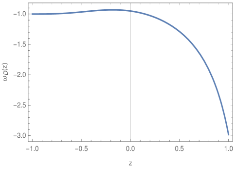
Figure 1: $\omega_{\mathrm{D}}(z)$ vs. $z$ for a particular set of values of the parameters from their viable ranges as per Eq.(41) and Eq.(51), say $\beta=0.35$, $\left(\alpha_{+}/\alpha_{-}\right)^{\beta}=10$, $\alpha_{+}/\beta=10^{-6}$ and $\gamma_{m}=1.8\times 10^{-4}$.

As a whole, we may argue that the entropic cosmology from the generalized entropy function $S_{\mathrm{g}}$ can unify the early inflation to the late dark energy era of the universe, for suitable ranges of the parameters given by:

$$\sigma_{0}= \,[0.013,0.017]\,,\quad\left(\alpha_{+}/\alpha_{-}\right)^{\beta}\geq 7.5\,,$$

$$\beta= \,(0,0.4]\ \mbox{and}\ \gamma_{m}=[1.5\times 10^{-4},2\times 10^{-4}]\,.$$ (53)

Despite these successes, here it deserves mentioning that the entropy function $S_{\mathrm{g}}$ seems to be plagued with singularity for certain cosmological evolution of the universe, in particular, in the context of bounce cosmology. Due to the reason that the Bekenstein-Hawking entropy can be expressed as $S=\pi/\left(GH^{2}\right)$, the generalized entropy $S_{\mathrm{g}}$ contains factor that is proportional to $1/H^{2}$ which diverges at $H=0$, for instance at the instant of bounce in the context of bounce cosmology. Therefore in a bounce scenario, the generalized entropy function shown in Eq.(9) is not physical, and thus, we need to search for a different generalized entropy function which can lead to various known entropy functions for suitable choices of the parameters, and at the same time, proves to be non-singular for the entire cosmological evolution of the universe even at $H=0$.

V Search for a singular-free generalized entropy

With this spirit, we propose a new singular-free entropy function given by OP-submitted ,

$$S_{\mathrm{ns}}\left[\alpha_{\pm},\beta,\gamma,\epsilon\right]=\frac{1}{\gamma}\bigg{[}\left\{1+\frac{1}{\epsilon}\tanh\left(\frac{\epsilon\alpha_{+}}{\beta}~{}S\right)\right\}^{\beta}-\left\{1+\frac{1}{\epsilon}\tanh\left(\frac{\epsilon\alpha_{-}}{\beta}~{}S\right)\right\}^{-\beta}\bigg{]}~{}~{},$$ (54)

where $\alpha_{\pm}$, $\beta$, $\gamma$ and $\epsilon$ are the parameters which are considered to be positive, $S$ symbolizes the Bekenstein-Hawking entropy and the suffix ’ns’ stands for ’non-singular’. In regard to the number of parameters, we propose a conjecture at the end of this section. First we demonstrate that the above entropy function remains finite, and thus is non-singular, during the whole cosmological evolution of a bouncing universe. In particular, the $S_{\mathrm{g}}$ takes the following form at the instant of bounce:

$$S_{\mathrm{ns}}\left[\alpha_{\pm},\beta,\gamma,\epsilon\right]=\frac{1}{\gamma}\bigg{[}\left\{1+\frac{1}{\epsilon}\right\}^{\beta}-\left\{1+\frac{1}{\epsilon}\right\}^{-\beta}\bigg{]}~{}~{}.$$ (55)

Having demonstrated the non-singular behaviour of the entropy function, we now show that $S_{\mathrm{ns}}$ of Eq.(54), for suitable choices of the parameters, reduces to various known entropies proposed so far.

• For $\epsilon\rightarrow 0$, $\alpha_{+}\rightarrow\infty$ and $\alpha_{-}=0$ along with the identification $\gamma=\left(\alpha_{+}/\beta\right)^{\beta}$, $S_{\mathrm{ns}}$ converges to the Tsallis entropy or to the Barrow entropy respectively.

• The limit $\epsilon\rightarrow 0$, $\alpha_{-}=0$, $\beta\rightarrow 0$ and $\frac{\alpha_{+}}{\beta}\rightarrow\mathrm{finite}$ results to the similarity between the non-singular generalized entropy $S_{\mathrm{g}}$ and the Rényi entropy.

• For $\epsilon\rightarrow 0$ and $\alpha_{-}\rightarrow 0$, the non-singular generalized entropy converges to the following form,

  $$S_{\mathrm{ns}}=\frac{1}{\gamma}\left[\left(1+\frac{\alpha_{+}}{\beta}~{}S\right)^{\beta}-1\right]$$ (56)

  Therefore with $\gamma=R$, $\alpha_{+}=R$ and $\beta=R/\delta$, the above form of $S_{\mathrm{ns}}$ becomes similar to the Sharma-Mittal entropy.

• For $\epsilon\rightarrow 0$, $\beta\rightarrow\infty$, $\alpha_{+}=\alpha_{-}=\frac{\gamma}{2}=K$ – the generalized entropy converges to the form of Kaniadakis entropy,

• Finally, $\epsilon\rightarrow 0$, $\alpha_{-}\rightarrow 0$, $\beta\rightarrow\infty$ and $\gamma=\alpha_{+}=(1-q)$, the generalized entropy of Eq. (54) gets resemble with the Loop Quantum Gravity entropy.

Furthermore, the generalized entropy function in Eq. (54) shares the following properties: (1) the non-singular generalized entropy satisfies the generalized third law of thermodynamics. (2) $S_{\mathrm{ns}}\left[\alpha_{\pm},\beta,\gamma,\epsilon\right]$ turns out to be a monotonically increasing function of $S$. (3) $S_{\mathrm{ns}}\left[\alpha_{\pm},\beta,\gamma,\epsilon\right]$ proves to converge to the Bekenstein-Hawking entropy at certain limit of the parameters.

At this stage it deserves mentioning that we have proposed two different generalized entropy functions in Eq.(9) and in Eq.(54) respectively – the former entropy function contains four independent parameters while the latter one has five parameters. Furthermore both the entropies are able to generalize the known entropies for suitable choices of the respective parameters. However as mentioned earlier that the entropy with four parameters becomes singular at $H=0$ (for instance, in a bounce scenario when the Hubble parameter vanishes at the instant of bounce), while the entropy function having five parameters proves to be singular-free during the whole cosmological evolution of the universe. Based on these findings, we give a second conjecture regarding the number of parameters in the non-singular generalized entropy function:

Conjecture - II: “The minimum number of parameters required in a generalized entropy function that can generalize all the known entropies, and at the same time, is also singular-free during the universe’s evolution – is equal to five”.

VI Cosmology with the non-singular generalized entropy

Applying the thermodynamic laws to the non-singular generalized entropy function $S_{\mathrm{ns}}$ and by following the same procedure as of Sec.[IV], one gets the cosmological field equations corresponding to the $S_{g}\mathrm{ns}$ OP-submitted :

$$\frac{1}{\gamma} \bigg{[} \alpha_{+}~{}\mathrm{sech}^{2}\left(\frac{\epsilon\pi\alpha_{+}}{\beta GH^{2}}\right)\left\{1+\frac{1}{\epsilon}\tanh\left(\frac{\epsilon\pi\alpha_{+}}{\beta GH^{2}}\right)\right\}^{\beta-1}$$ (57)

$$+ \alpha_{-}~{}\mathrm{sech}^{2}\left(\frac{\epsilon\pi\alpha_{-}}{\beta GH^{2}}\right)\left\{1+\frac{1}{\epsilon}\tanh\left(\frac{\epsilon\pi\alpha_{-}}{\beta GH^{2}}\right)\right\}^{-\beta-1}\bigg{]}\dot{H}=-4\pi G\left(\rho+p\right)~{}~{}.$$

Owing to the conservation equation of matter fields, in particular $\dot{\rho}+3H\left(\rho+p\right)=0$, the above expression can be integrated to get

$$f\left(H;~{}\alpha_{\pm},\beta,\gamma,\epsilon\right)=\frac{8\pi G\rho}{3}+\frac{\Lambda}{3}\,.$$ (58)

Here the integration constant is symbolized by $\Lambda$ and the function $f$ has the following form:

$$f\left(H;~{}\alpha_{\pm},\beta,\gamma,\epsilon\right)=\frac{2}{\gamma}\int \bigg{[} \alpha_{+}~{}\mathrm{sech}^{2}\left(\frac{\epsilon\pi\alpha_{+}}{\beta GH^{2}}\right)\left\{1+\frac{1}{\epsilon}\tanh\left(\frac{\epsilon\pi\alpha_{+}}{\beta GH^{2}}\right)\right\}^{\beta-1}$$ (59)

$$+ \alpha_{-}~{}\mathrm{sech}^{2}\left(\frac{\epsilon\pi\alpha_{-}}{\beta GH^{2}}\right)\left\{1+\frac{1}{\epsilon}\tanh\left(\frac{\epsilon\pi\alpha_{-}}{\beta GH^{2}}\right)\right\}^{-\beta-1}\bigg{]}H~{}dH~{}~{}.$$

In regard to the functional form of $f\left(H;~{}\alpha_{\pm},\beta,\gamma,\epsilon\right)$, we would like to mention that the integration in Eq.(59) may not be performed in a closed form, unless certain conditions are imposed. For example, we consider $GH^{2}\ll 1$ which is, in fact, valid during the universe’s evolution (i.e the Hubble parameter is less than the Planck scale). With $GH^{2}\ll 1$, the functional form of $f$ turns out to be,

$$f\left(H;~{}\alpha_{\pm},\beta,\gamma,\epsilon\right)=\frac{4}{\gamma}H^{2} \bigg{\{} \alpha_{+}\left(1+\frac{1}{\epsilon}\right)^{\beta-1}\left[\mathrm{exp}\left(-\frac{2\epsilon\pi\alpha_{+}}{\beta GH^{2}}\right)+\left(\frac{2\epsilon\pi\alpha_{+}}{\beta GH^{2}}\right)\mathrm{Ei}\left(-\frac{2\epsilon\pi\alpha_{+}}{\beta GH^{2}}\right)\right]$$ (60)

$$+ \alpha_{-}\left(1+\frac{1}{\epsilon}\right)^{-\beta-1}\left[\mathrm{exp}\left(-\frac{2\epsilon\pi\alpha_{-}}{\beta GH^{2}}\right)+\left(\frac{2\epsilon\pi\alpha_{-}}{\beta GH^{2}}\right)\mathrm{Ei}\left(-\frac{2\epsilon\pi\alpha_{-}}{\beta GH^{2}}\right)\right]\bigg{\}}~{}~{}.$$

Therefore as a whole, Eq. (57) and Eq. (58) are the cosmological field equations corresponding to the generalized entropy $S_{\mathrm{g}}$.

VI.1 Non-singular entropy on bounce cosmology

In this section, we will address the implications of the generalized entropy $S_{\mathrm{ns}}$ on non-singular bounce cosmology, in particular, we will investigate whether the entropic energy density can trigger a viable bounce during the early stage of the universe that is consistent with the observational constraints. For this purpose, we take the matter field and the cosmological constant to be absent, i.e., $\rho=p=\Lambda=0$. In effect, Eq. (57) becomes,

$$\frac{1}{\gamma} \bigg{[} \alpha_{+}~{}\mathrm{sech}^{2}\left(\frac{\epsilon\pi\alpha_{+}}{\beta GH^{2}}\right)\left\{1+\frac{1}{\epsilon}\tanh\left(\frac{\epsilon\pi\alpha_{+}}{\beta GH^{2}}\right)\right\}^{\beta-1}$$ (61)

$$+ \alpha_{-}~{}\mathrm{sech}^{2}\left(\frac{\epsilon\pi\alpha_{-}}{\beta GH^{2}}\right)\left\{1+\frac{1}{\epsilon}\tanh\left(\frac{\epsilon\pi\alpha_{-}}{\beta GH^{2}}\right)\right\}^{-\beta-1}\bigg{]}\dot{H}=0~{}~{}.$$

The parameters $\left(\alpha_{\pm},\beta,\gamma,\epsilon\right)$ are positive, and thus the solution of the above equation is given by: $\dot{H}=0$ or equivalently $H=\mathrm{constant}$. Clearly $H=\mathrm{constant}$ does not lead to the correct evolution of the universe. Thus similar to the previous case, we consider the parameters of $S_{\mathrm{ns}}[\alpha_{\pm},\beta,\gamma,\epsilon]$ vary with time. In particular, we consider the parameter $\gamma$ to vary with time, and all the other parameters remain fixed, i.e.

$$\gamma=\gamma(N)~{}~{},$$ (62)

with $N$ being the e-fold number of the universe. In such scenario where $\gamma(N)$ varies with time, the Friedmann equation corresponds to $S_{\mathrm{ns}}[\alpha_{\pm},\beta,\gamma,\epsilon]$ gets modified compared to Eq.(61), and is given by:

$$\left[\frac{\alpha_{+}~{}\mathrm{sech}^{2}\left(\frac{\epsilon\alpha_{+}}{\beta}S\right)\left\{1+\frac{1}{\epsilon}\tanh\left(\frac{\epsilon\alpha_{+}}{\beta}S\right)\right\}^{\beta-1}+\alpha_{-}~{}\mathrm{sech}^{2}\left(\frac{\epsilon\alpha_{-}}{\beta}S\right)\left\{1+\frac{1}{\epsilon}\tanh\left(\frac{\epsilon\alpha_{-}}{\beta}S\right)\right\}^{-\beta-1}}{\left\{1+\frac{1}{\epsilon}\tanh\left(\frac{\epsilon\alpha_{+}}{\beta}S\right)\right\}^{\beta}-\left\{1+\frac{1}{\epsilon}\tanh\left(\frac{\epsilon\alpha_{-}}{\beta}S\right)\right\}^{-\beta}}\right]dS=\frac{\gamma^{\prime}(N)}{\gamma(N)}dN$$ (63)

where an overprime denotes $\frac{d}{d\eta}$. Eq.(63) can be integrated to get,

$$\tanh{\left(\frac{\epsilon\pi\alpha}{\beta GH^{2}}\right)}=\left\{\frac{\gamma(N)+\sqrt{\gamma^{2}(N)+4}}{2}\right\}^{1/\beta}-1~{}~{}.$$ (64)

where we take $\alpha_{+}=\alpha_{-}=\alpha$ (say, without losing any generality) in order to extract an explicit solution of $H(N)$. Due to the appearance of quadratic power of $H$, Eq.(64) allows a positive branch as well as a negative branch of the Hubble parameter. This leads to a natural possibility of symmetric bounce in the present context of singular free generalized entropic cosmology. Moreover Eq.(64) also demonstrates that the explicit evolution of $H(N)$ does depend on the form of $\gamma(N)$. In the following, we will consider two cases where we will determine the form of $\gamma(N)$ such that it gives two different symmetric bounce scenarios respectively.

1. The exponential bounce described by the scale factor,

   $$a(t)=\mathrm{exp}\left(a_{0}t^{2}\right)~{}~{}.$$ (65)

   This results to a symmetric bounce at $t=0$. Here $a_{0}$ is a constant having mass dimension [+2] – this constant is related with the entropic parameters of $S_{\mathrm{ns}}$ and thus, without losing any generality, we take $a_{0}=\frac{\epsilon\pi\alpha}{4G\beta}$. Such an exponential bounce can be achieved from singular free entropic cosmology provided the $\gamma(N)$ is given by,

   $$\gamma(N)=\left\{1+\frac{1}{\epsilon}\tanh\left(\frac{1}{N}\right)\right\}^{\beta}-\left\{1+\frac{1}{\epsilon}\tanh\left(\frac{1}{N}\right)\right\}^{-\beta}~{}~{}.$$ (66)

2. The quasi-matter bounce is described by, In this case, the scale factor is,

   $$a(t)=\left[1+a_{0}\left(\frac{t}{t_{0}}\right)^{2}\right]^{n}$$ (67)

   which is symmetric about $t=0$ when the bounce happens. The $n$, $a_{0}$ and $t_{0}$ considered in the scale factor are related to the entropic parameters, and we take it as follows:

   $$n=\sqrt{\alpha}~{}~{}~{}~{}~{}~{},~{}~{}~{}~{}~{}~{}~{}~{}a_{0}=\frac{\pi}{4\beta}~{}~{}~{}~{}~{}~{}~{}~{}\mathrm{and}~{}~{}~{}~{}~{}~{}~{}~{}~{}t_{0}=\sqrt{G/\epsilon}~{}~{},$$ (68)

   with $G$ being the gravitational constant. The relation between ($n$, $a_{0}$, $t_{0}$) with the entropic parameters can be considered in a different way compared to the Eq.(68), however for a simplified expression of $\gamma(N)$ we consider the relations as of Eq.(68). Consequently the $\gamma(N)$ which leads to such quasi-matter bounce, comes as,

   $$\gamma(N)=\left\{1+\frac{1}{\epsilon}\tanh\left[\mathrm{e}^{-N/\sqrt{\alpha}}\left(\mathrm{e}^{N/\sqrt{\alpha}}-1\right)^{\frac{1}{2}}\right]\right\}^{\beta}-\left\{1+\frac{1}{\epsilon}\tanh\left[\mathrm{e}^{-N/\sqrt{\alpha}}\left(\mathrm{e}^{N/\sqrt{\alpha}}-1\right)^{\frac{1}{2}}\right]\right\}^{-\beta}~{}~{}.$$ (69)

Here it deserves mentioning that in the case of exponential bounce, the comoving Hubble radius asymptotically goes to zero and thus the perturbation modes remain at the super-Hubble regime at the distant past. This may results to the “horizon problem” in the exponential bounce scenario. On contrary, the comoving Hubble radius in the case of quasi-matter bounce asymptotically diverges to infinity at both sides of the bounce, and thus the perturbation modes lie within the deep sub-Hubble regime at the distant past – this resolves the horizon issue. Based on this arguments, we will concentrate on the quasi-matter bounce to perform the perturbation analysis.

In regard to the perturbation analysis, we represent the present entropic cosmology with the ghost free Gauss-Bonnet (GB) theory of gravity proposed in Nojiri:2018ouv . The motivation of such representation is due to the rich structure of the Gauss-Bonnet theory in various directions of cosmology Odintsov:2022unp ; Elizalde:2020zcb ; Bamba:2020qdj ; Nojiri:2022xdo . The action for $f(\mathcal{G})$ gravity is given by Nojiri:2018ouv ,

$$S=\int d^{4}x\sqrt{-g}\left(\frac{1}{2\kappa^{2}}R+\lambda\left(\frac{1}{2}\partial_{\mu}\chi\partial^{\mu}\chi+\frac{\mu^{4}}{2}\right)-\frac{1}{2}\partial_{\mu}\chi\partial^{\mu}\chi+h\left(\chi\right)\mathcal{G}-V\left(\chi\right)\right)\,,$$ (70)

where $\mu$ is a constant having mass dimension $[+1]$, $\lambda$ represents the Lagrange multiplier, $\chi$ is a scalar field and $V(\chi)$ is its potential. Moreover $\mathcal{G}=R^{2}-4R_{\mu\nu}R^{\mu\nu}+R_{\mu\nu\alpha\beta}R^{\mu\nu\alpha\beta}$ is the Gauss-Bonnet scalar and $h(\chi)$ symbolizes the Gauss-Bonnet coupling with the scalar field. Moreover we consider such class of Gauss-Bonnet coupling functions that satisfy $\ddot{h}=\dot{h}H$. This condition actually leads to the speed of the gravitational wave as unity in the context of GB theory and makes the model compatible with the GW170817 event. For a certain $\gamma(N)$ in the context of entropic cosmology, there exists an equivalent set of GB parameters in the side of Gauss-Bonnet cosmology that results to the same cosmological evolution as of the generalized entropy. In particular, the equivalent forms of $\tilde{V}(\chi)$ and $\lambda(t)$ for a certain $\gamma(N)$ turn out to be,

$$\tilde{V}(\chi) = -8\pi G~{}F_{1}\left[\gamma(N),\gamma^{\prime}(N)\right]\left(\frac{1}{\kappa^{2}}+8h_{0}a(t)H(t)\right)\bigg{|}_{t=\chi/\mu^{2}}\,,$$ (71)

$$\mu^{4}\lambda(t) = -8\pi G~{}F_{2}\left[\gamma(N),\gamma^{\prime}(N)\right]\left(\frac{1}{\kappa^{2}}-8h_{0}a(t)H(t)\right)\,,$$ (72)

where the functions $F_{1}\left[\gamma(N),\gamma^{\prime}(N)\right]$ and $F_{2}\left[\gamma(N),\gamma^{\prime}(N)\right]$ are given by,

$$F_{1}\left[\gamma(N),\gamma^{\prime}(N)\right] = -\left(\frac{3\epsilon\alpha}{4\beta G^{2}}\right)\left[\ln{\left\{\frac{1}{2\left(\frac{2}{\gamma(N)+\sqrt{\gamma^{2}(N)+4}}\right)^{1/\beta}-1}\right\}}\right]^{-1}+H^{4}\left(\frac{\gamma^{\prime}(N)}{8\pi^{2}\gamma(N)}\right)\times$$

$$\Bigg{[} \frac{\left\{1+\frac{1}{\epsilon}\tanh\left(\frac{\epsilon\pi\alpha}{\beta GH^{2}}\right)\right\}^{\beta}-\left\{1+\frac{1}{\epsilon}\tanh\left(\frac{\epsilon\pi\alpha}{\beta GH^{2}}\right)\right\}^{-\beta}}{\alpha~{}\mathrm{sech}^{2}\left(\frac{\epsilon\pi\alpha}{\beta GH^{2}}\right)\left[\left\{1+\frac{1}{\epsilon}\tanh\left(\frac{\epsilon\pi\alpha}{\beta GH^{2}}\right)\right\}^{\beta-1}+\left\{1+\frac{1}{\epsilon}\tanh\left(\frac{\epsilon\pi\alpha}{\beta GH^{2}}\right)\right\}^{-\beta-1}\right]}\Bigg{]}$$

and

$$F_{2}\left[\gamma(N),\gamma^{\prime}(N)\right]=H^{4}\left(\frac{\gamma^{\prime}(N)}{8\pi^{2}\gamma(N)}\right)\left[\frac{\left\{1+\frac{1}{\epsilon}\tanh\left(\frac{\epsilon\pi\alpha}{\beta GH^{2}}\right)\right\}^{\beta}-\left\{1+\frac{1}{\epsilon}\tanh\left(\frac{\epsilon\pi\alpha}{\beta GH^{2}}\right)\right\}^{-\beta}}{\alpha~{}\mathrm{sech}^{2}\left(\frac{\epsilon\pi\alpha}{\beta GH^{2}}\right)\left[\left\{1+\frac{1}{\epsilon}\tanh\left(\frac{\epsilon\pi\alpha}{\beta GH^{2}}\right)\right\}^{\beta-1}+\left\{1+\frac{1}{\epsilon}\tanh\left(\frac{\epsilon\pi\alpha}{\beta GH^{2}}\right)\right\}^{-\beta-1}\right]}\right]$$

respectively. Based on Eq.(71) and Eq.(72), we may argue that the entropic cosmology of $S_{\mathrm{ns}}$ can be equivalently represented by Gauss-Bonnet cosmology.

As mentioned earlier that we consider the quasi-matter bounce scenario described by the scale factor (67) to analyze the perturbation, where the perturbation modes generate during the contracting phase deep in the sub-Hubble regime, which in turn ensures the resolution of the horizon problem. The important quantities that we will need are,

$$Q_{a} = -8\dot{h}H^{2}=-\frac{4n^{2}(1+2n)\sqrt{\widetilde{R}}}{\pi G}\left(\frac{\widetilde{R}}{R_{0}}\right)^{\frac{1}{2}-n}~{}~{}~{}~{}~{},~{}~{}~{}~{}~{}~{}Q_{b}=-16\dot{h}H=\frac{4n(1+2n)}{\pi G}\left(\frac{\widetilde{R}}{R_{0}}\right)^{\frac{1}{2}-n}\,,$$

$$Q_{c} = Q_{d}=0~{}~{}~{}~{},~{}~{}~{}~{}~{}Q_{e}=-32\dot{h}\dot{H}=\frac{8n(1+2n)\sqrt{\widetilde{R}}}{\pi G}\left(\frac{\widetilde{R}}{R_{0}}\right)^{\frac{1}{2}-n}~{}~{}~{}~{},~{}~{}~{}~{}Q_{f}=16\left[\ddot{h}-\dot{h}H\right]=0\,,$$ (73)

respectively, where $R_{0}=\frac{1}{t_{0}^{2}}$ and $\widetilde{R}(t)=\frac{R(t)}{12n(1-4n)}$. In regard to curvature perturbation, the Mukhanov-Sasaki (MS) equation in Fourier mode comes as,

$$\frac{d^{2}v_{k}(\eta)}{d\eta^{2}}+\left(k^{2}-\frac{\sigma}{\eta^{2}}\right)v_{k}(\eta)=0\,,$$ (74)

here $\eta$ symbolizes the conformal time coordinate and $v(k,\eta)$ is the scalar MS variable. Moreover $\sigma$ is given by,

$$\sigma=\xi(\xi-1)\left[1+24\left(1-4n^{2}\right)\left(\frac{\widetilde{R}}{R_{0}}\right)^{\frac{1}{2}-n}\right]\,,$$ (75)

which is approximately a constant during the generation era of the perturbation modes in the sub-Hubble regime during the contracting phase, due to the condition $n<1/2$ (required to solve the horizon problem). In effect of which and considering the Bunch-Davies initial condition, the scalar power spectrum $\mathcal{P}_{\Psi}(k,\eta)$ in the super-horizon scale becomes,

$$\mathcal{P}_{\Psi}(k,\eta)=\left[\left(\frac{1}{2\pi}\right)\frac{1}{z\left|\eta\right|}\frac{\Gamma(\nu)}{\Gamma(3/2)}\right]^{2}\left(\frac{k|\eta|}{2}\right)^{3-2\nu}\,,$$ (76)

In regard to the tensor perturbation, the Mukhanov-Sasaki equation takes the following form,

$$\frac{d^{2}v_{T}(k,\eta)}{d\eta^{2}}+\left(k^{2}-\frac{\sigma_{T}}{\eta^{2}}\right)v_{T}(k,\eta)=0\,,$$ (77)

where $v_{T}(k,\eta)$ being the Fourier mode for the tensor MS variable, and $\sigma_{T}$ has the following form,

$$\sigma_{T}=\xi(\xi-1)\left[1-16(1-4n^{2})\left(\frac{\widetilde{R}}{R_{0}}\right)^{\frac{1}{2}-n}\right]\,.$$ (78)

Due to $n<1/2$, the quantity $\sigma_{T}$ can be safely considered to be a constant during the generation era of the perturbation modes at the contracting phase of the universe. Here it may be mentioned that both the tensor polarization modes ($+$ and $\times$ polarization modes) obey the same evolution Eq.(77) – this means that the two polarization modes equally contribute to the energy density of the tensor perturbation variable, and thus we will multiply by the factor ’2’ in the final expression of the tensor power spectrum. Similar to the curvature perturbation variable, the tensor perturbation initiates from the Bunch-Davies vacuum at the distant past, i.e. $v_{T}(k,\eta)$, i.e $\lim_{k|\eta|\gg 1}v_{T}(k,\eta)=\frac{1}{\sqrt{2k}}e^{-ik\eta}$. With such initial condition, we obtain the tensor power spectrum for $k$th mode in the super-Hubble regime as,

$$\mathcal{P}_{T}(k,\tau)=2\left[\frac{1}{2\pi}\frac{1}{z_{T}\left|\eta\right|}\frac{\Gamma(\theta)}{\Gamma(3/2)}\right]^{2}\left(\frac{k|\eta|}{2}\right)^{3-2\theta}\,,$$ (79)

where $\theta=\sqrt{\sigma_{T}+\frac{1}{4}}$. Having obtained the scalar and tensor power spectra, we determine $n_{s}$ and $r$, and they are given by (the suffix ’h’ with a quantity represents the quantity at the instant of horizon crossing),

$$n_{s}=4-\sqrt{1+4\sigma_{h}}\,,\quad r=2\left[\frac{z(\eta_{h})}{z_{T}(\eta_{h})}\frac{\Gamma(\theta)}{\Gamma(\nu)}\right]^{2}\left(k\left|\eta_{h}\right|\right)^{2(\nu-\theta)}\,,$$ (80)

where the quantities have the following forms,

$$\nu= \sqrt{\sigma_{h}+\frac{1}{4}}\,;\quad\sigma_{h}=\xi(\xi-1)\left[1+24\left(1-4n^{2}\right)\left(\frac{\widetilde{R}_{h}}{R_{0}}\right)^{\frac{1}{2}-n}\right]\,,$$

$$\theta= \sqrt{\sigma_{T,h}+\frac{1}{4}}\,;\quad\sigma_{T,h}=\xi(\xi-1)\left[1-16(1-4n^{2})\left(\frac{\widetilde{R}_{h}}{R_{0}}\right)^{\frac{1}{2}-n}\right]\,,$$

$$z(\eta_{h})= -\frac{1}{\sqrt{n}}\left(\frac{a_{0}^{n}}{\kappa\widetilde{R}_{h}^{n}}\right)\left[1-24n(1+2n)\left(\frac{\widetilde{R}_{h}}{R_{0}}\right)^{\frac{1}{2}-n}\right]\,,$$

$$z_{T}(\eta_{h})= \frac{1}{\sqrt{2}}\left(\frac{a_{0}^{n}}{\kappa\widetilde{R}_{h}^{n}}\right)\left[1+16n(1+2n)\left(\frac{\widetilde{R}_{h}}{R_{0}}\right)^{\frac{1}{2}-n}\right]\,.$$ (81)

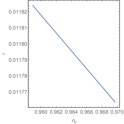
Figure 2: Parametric plot of $n_{s}$ (along $x$-axis) vs. $r$ (along $y$-axis) with respect to $n$. Here we take $\alpha=[0.0938,0.0939]$ and $\beta=\frac{\pi}{16}$.

Here $\widetilde{R}_{h}$ represents the Ricci scalar at the horizon crossing, and using the horizon crossing condition $k\eta_{h}=\frac{2n}{1-2n}$, it comes as,

$$\widetilde{R}_{h}=\left[\frac{1}{26na_{0}^{n}}\right]^{2/(1-2n)}\mathrm{By}^{-2}\,.$$ (82)

Therefore it is clear that $n_{s}$ and $r$ in the present context depends on the parameters $n$ and $a_{0}$. Here we need to recall that $n$ and $a_{0}$ are related to the entropic parameters as $n=\sqrt{\alpha}$ and $a_{0}=\pi/\left(4\beta\right)$ respectively. It turns out that the theoretical predictions for $n_{s}$ and $r$ get simultaneously compatible with the recent Planck data for a small range of the entropic parameters given by: $\alpha=[0.0938,0.0939]$ and $\beta=\frac{\pi}{16}$, see Fig.[2].

VII Conclusion

In this short review article, we have proposed generalized entropic function(s) and have addressed their implications on black hole thermodynamics as well as on cosmology. In the first half of the paper, a 4-parameter and a 3-parameter generalized entropy functions are shown, which are able to generalize the known entropies proposed so far, like the Tsallis, Rényi, Barrow, Sharma-Mittal, Kaniadakis and Loop Quantum Gravity entropies for suitable choices of the respective entropic parameters. However the 4-parameter entropy functions proves to be more general compared to the 3-parameter entropy function, in particular, the 3-parameter entropy does not converge to the Kaniadakis entropy for any choices of the parameters, unlike to the entropy having 4 parameters which generalizes all the known entropies including the Kaniadakis one. Thus regarding to the number of parameters in a generalized entropy function, we have provided a conjecture – “The minimum number of parameters required in a generalized entropy function that can generalize all the known entropies mentioned above is equal to four”. Consequently the interesting implications of 3-parameter entropy on black hole thermodynamics and the 4-parameter entropy on cosmology have been addressed. It turns out that the entropic cosmology corresponding to the 4-parameter generalized entropy results to an unified cosmological scenario of early inflation and the late dark energy era of the universe, where the observable quantities are found to be compatible with the recent Planck data for certain viable ranges of the entropic parameters.

Despite these successes, here it deserves mentioning that the 4-parameter entropy function ($S_{\mathrm{g}}$) seems to be plagued with singularity for certain cosmological evolution of the universe. In particular, $S_{\mathrm{g}}$ diverges at the instant when the Hubble parameter vanishes, for instance at the instant of bounce in the context of bounce cosmology. With this spirit, we have proposed a singular-free 5-parameter entropy function ($S_{\mathrm{ns}}$) which converges to all the known entropy functions for particular limits of the entropic parameters, and at the same time, also proves to be non-singular for the entire cosmological evolution of the universe even at $H=0$ (where $H$ represents the Hubble parameter). Regarding to the non-singular entropy, a second conjecture has been given : “The minimum number of parameters required in a generalized entropy function that can generalize all the known entropies, and at the same time, is also singular-free during the universe’s evolution – is equal to five”. Such non-singular behaviour of $S_{\mathrm{ns}}$ proves to be useful in describing the bounce cosmology, in particular, the entropic cosmology corresponding to $S_{\mathrm{ns}}$ naturally allows symmetric bounce universe. With the perturbation analysis in the context of entropic bounce, it has been shown that the observable quantities like the spectral tilt and the tensor-to-scalar ratio are simultaneously compatible with the Planck data in the background of symmetric quasi-matter bounce scenario.

Finally we would like to mention that the proposals of generalized entropy functions ($S_{\mathrm{g}}$ or $S_{\mathrm{ns}}$) opens a new directions in theoretical physics, and its vast consequences may hint some unexplored directions of black hole thermodynamics as well as of cosmology. For example, it will be of utmost interest to study the aspects of the generalized entropy functions on primordial black hole formation or primordial gravitational wave or the recently found astrophysical black holes as well. With the recent and future advancements of different detectors (like the GW detectors or regarding the black hole detection), we hope that these study can indirectly quantify the viable ranges of entropic parameters.

References

- (1) J. D. Bekenstein, Phys. Rev. D 7 (1973), 2333-2346 doi:10.1103/PhysRevD.7.2333
- (2) S. W. Hawking, Commun. Math. Phys. 43 (1975), 199-220 [erratum: Commun. Math. Phys. 46 (1976), 206] doi:10.1007/BF02345020
- (3) J. M. Bardeen, B. Carter and S. W. Hawking, Commun. Math. Phys. 31 (1973), 161-170 doi:10.1007/BF01645742
- (4) R. M. Wald, Living Rev. Rel. 4 (2001), 6 doi:10.12942/lrr-2001-6 [arXiv:gr-qc/9912119 [gr-qc]].
- (5) C. Tsallis, J. Statist. Phys. 52 (1988), 479-487 doi:10.1007/BF01016429
- (6) A. Rényi, Proceedings of the Fourth Berkeley Symposium on Mathematics, Statistics and Probability, University of California Press (1960), 547-56.
- (7) J. D. Barrow, Phys. Lett. B 808 (2020), 135643 doi:10.1016/j.physletb.2020.135643 [arXiv:2004.09444 [gr-qc]].
- (8) A. Sayahian Jahromi, S. A. Moosavi, H. Moradpour, J. P. Morais Graça, I. P. Lobo, I. G. Salako and A. Jawad, Phys. Lett. B 780 (2018), 21-24 doi:10.1016/j.physletb.2018.02.052 [arXiv:1802.07722 [gr-qc]].
- (9) G. Kaniadakis, Phys. Rev. E 72 (2005), 036108 doi:10.1103/PhysRevE.72.036108 [arXiv:cond-mat/0507311 [cond-mat]].
- (10) A. Majhi, Phys. Lett. B 775 (2017), 32-36 doi:10.1016/j.physletb.2017.10.043 [arXiv:1703.09355 [gr-qc]].
- (11) E. Witten, Adv. Theor. Math. Phys. 2 (1998), 253-291 doi:10.4310/ATMP.1998.v2.n2.a2 [arXiv:hep-th/9802150 [hep-th]].
- (12) L. Susskind and E. Witten, [arXiv:hep-th/9805114 [hep-th]].
- (13) W. Fischler and L. Susskind, [arXiv:hep-th/9806039 [hep-th]].
- (14) S. Nojiri, S. D. Odintsov and T. Paul, Symmetry 13 (2021) no.6, 928 doi:10.3390/sym13060928 [arXiv:2105.08438 [gr-qc]].
- (15) S. Nojiri, S. D. Odintsov and T. Paul, Phys. Lett. B 825 (2022), 136844 doi:10.1016/j.physletb.2021.136844 [arXiv:2112.10159 [gr-qc]].
- (16) M. Li, Phys. Lett. B 603 (2004) 1 doi:10.1016/j.physletb.2004.10.014 [hep-th/0403127].
- (17) M. Li, X. D. Li, S. Wang and Y. Wang, Commun. Theor. Phys. 56 (2011), 525-604 doi:10.1088/0253-6102/56/3/24 [arXiv:1103.5870 [astro-ph.CO]].
- (18) S. Wang, Y. Wang and M. Li, Phys. Rept. 696 (2017) 1 doi:10.1016/j.physrep.2017.06.003 [arXiv:1612.00345 [astro-ph.CO]].
- (19) D. Pavon and W. Zimdahl, Phys. Lett. B 628 (2005) 206 doi:10.1016/j.physletb.2005.08.134 [gr-qc/0505020].
- (20) S. Nojiri and S. D. Odintsov, Gen. Rel. Grav. 38 (2006) 1285 doi:10.1007/s10714-006-0301-6 [hep-th/0506212].
- (21) R. G. Landim, Phys. Rev. D 106 (2022) no.4, 043527 doi:10.1103/PhysRevD.106.043527 [arXiv:2206.10205 [astro-ph.CO]].
- (22) X. Zhang, Int. J. Mod. Phys. D 14 (2005) 1597 doi:10.1142/S0218271805007243 [astro-ph/0504586].
- (23) B. Guberina, R. Horvat and H. Stefancic, JCAP 0505 (2005) 001 doi:10.1088/1475-7516/2005/05/001 [astro-ph/0503495].
- (24) E. Elizalde, S. Nojiri, S. D. Odintsov and P. Wang, Phys. Rev. D 71 (2005) 103504 doi:10.1103/PhysRevD.71.103504 [hep-th/0502082].
- (25) M. Ito, Europhys. Lett. 71 (2005) 712 doi:10.1209/epl/i2005-10151-x [hep-th/0405281].
- (26) Y. g. Gong, B. Wang and Y. Z. Zhang, Phys. Rev. D 72 (2005) 043510 doi:10.1103/PhysRevD.72.043510 [hep-th/0412218].
- (27) M. Bouhmadi-Lopez, A. Errahmani and T. Ouali, Phys. Rev. D 84 (2011) 083508 doi:10.1103/PhysRevD.84.083508 [arXiv:1104.1181 [astro-ph.CO]].
- (28) M. Malekjani, Astrophys. Space Sci. 347 (2013) 405 doi:10.1007/s10509-013-1522-2 [arXiv:1209.5512 [gr-qc]].
- (29) M. Khurshudyan, Astrophys. Space Sci. 361 (2016) no.12, 392 doi:10.1007/s10509-016-2981-z
- (30) R. C. G. Landim, Int. J. Mod. Phys. D 25 (2016) no.04, 1650050 doi:10.1142/S0218271816500504 [arXiv:1508.07248 [hep-th]].
- (31) C. Gao, F. Wu, X. Chen and Y. G. Shen, Phys. Rev. D 79 (2009) 043511 doi:10.1103/PhysRevD.79.043511 [arXiv:0712.1394 [astro-ph]].
- (32) M. Li, C. Lin and Y. Wang, JCAP 0805 (2008) 023 doi:10.1088/1475-7516/2008/05/023 [arXiv:0801.1407 [astro-ph]].
- (33) F. K. Anagnostopoulos, S. Basilakos and E. N. Saridakis, [arXiv:2005.10302 [gr-qc]].
- (34) X. Zhang and F. Q. Wu, Phys. Rev. D 72 (2005) 043524 doi:10.1103/PhysRevD.72.043524 [astro-ph/0506310].
- (35) M. Li, X. D. Li, S. Wang and X. Zhang, JCAP 0906 (2009) 036 doi:10.1088/1475-7516/2009/06/036 [arXiv:0904.0928 [astro-ph.CO]].
- (36) C. Feng, B. Wang, Y. Gong and R. K. Su, JCAP 0709 (2007) 005 doi:10.1088/1475-7516/2007/09/005 [arXiv:0706.4033 [astro-ph]].
- (37) X. Zhang, Phys. Rev. D 79 (2009) 103509 doi:10.1103/PhysRevD.79.103509 [arXiv:0901.2262 [astro-ph.CO]].
- (38) J. Lu, E. N. Saridakis, M. R. Setare and L. Xu, JCAP 1003 (2010) 031 doi:10.1088/1475-7516/2010/03/031 [arXiv:0912.0923 [astro-ph.CO]].
- (39) S. M. R. Micheletti, JCAP 1005 (2010) 009 doi:10.1088/1475-7516/2010/05/009 [arXiv:0912.3992 [gr-qc]].
- (40) P. Mukherjee, A. Mukherjee, H. Jassal, A. Dasgupta and N. Banerjee, Eur. Phys. J. Plus 134 (2019) no.4, 147 doi:10.1140/epjp/i2019-12504-7 [arXiv:1710.02417 [astro-ph.CO]].
- (41) S. Nojiri and S. Odintsov, Eur. Phys. J. C 77 (2017) no.8, 528 doi:10.1140/epjc/s10052-017-5097-x [arXiv:1703.06372 [hep-th]].
- (42) S. Nojiri, S. D. Odintsov and E. N. Saridakis, Eur. Phys. J. C 79 (2019) no.3, 242 [arXiv:1903.03098 [gr-qc]].
- (43) E. N. Saridakis, Phys. Rev. D 102 (2020) no.12, 123525 doi:10.1103/PhysRevD.102.123525 [arXiv:2005.04115 [gr-qc]].
- (44) J. D. Barrow, S. Basilakos and E. N. Saridakis, Phys. Lett. B 815 (2021), 136134 doi:10.1016/j.physletb.2021.136134 [arXiv:2010.00986 [gr-qc]].
- (45) P. Adhikary, S. Das, S. Basilakos and E. N. Saridakis, [arXiv:2104.13118 [gr-qc]].
- (46) S. Srivastava and U. K. Sharma, Int. J. Geom. Meth. Mod. Phys. 18 (2021) no.01, 2150014 doi:10.1142/S0219887821500146 [arXiv:2010.09439 [physics.gen-ph]].
- (47) V. K. Bhardwaj, A. Dixit and A. Pradhan, New Astron. 88 (2021), 101623 doi:10.1016/j.newast.2021.101623 [arXiv:2102.09946 [gr-qc]].
- (48) G. Chakraborty and S. Chattopadhyay, Int. J. Mod. Phys. D 29 (2020) no.03, 2050024 doi:10.1142/S0218271820500248 [arXiv:2006.07142 [physics.gen-ph]].
- (49) A. Sarkar and S. Chattopadhyay, Int. J. Geom. Meth. Mod. Phys. 18 (2021) no.09, 2150148 doi:10.1142/S0219887821501486
- (50) S. Nojiri, S. D. Odintsov and V. Faraoni, Phys. Rev. D 105 (2022) no.4, 044042 doi:10.1103/PhysRevD.105.044042 [arXiv:2201.02424 [gr-qc]].
- (51) S. Nojiri, S. D. Odintsov and T. Paul, Phys. Lett. B 831 (2022), 137189 doi:10.1016/j.physletb.2022.137189 [arXiv:2205.08876 [gr-qc]].
- (52) S. D. Odintsov and T. Paul, [arXiv:2212.05531 [gr-qc]].
- (53) R. Horvat, Phys. Lett. B 699 (2011), 174-176 doi:10.1016/j.physletb.2011.04.004 [arXiv:1101.0721 [hep-ph]].
- (54) S. Nojiri, S. D. Odintsov and E. N. Saridakis, Phys. Lett. B 797 (2019), 134829 doi:10.1016/j.physletb.2019.134829 [arXiv:1904.01345 [gr-qc]].
- (55) T. Paul, EPL 127 (2019) no.2, 20004 doi:10.1209/0295-5075/127/20004 [arXiv:1905.13033 [gr-qc]].
- (56) A. Bargach, F. Bargach, A. Errahmani and T. Ouali, Int. J. Mod. Phys. D 29 (2020) no.02, 2050010 doi:10.1142/S0218271820500108 [arXiv:1904.06282 [hep-th]].
- (57) E. Elizalde and A. Timoshkin, Eur. Phys. J. C 79 (2019) no.9, 732 doi:10.1140/epjc/s10052-019-7244-z [arXiv:1908.08712 [gr-qc]].
- (58) A. Oliveros and M. A. Acero, EPL 128 (2019) no.5, 59001 doi:10.1209/0295-5075/128/59001 [arXiv:1911.04482 [gr-qc]].
- (59) A. Mohammadi, [arXiv:2203.06643 [gr-qc]].
- (60) G. Chakraborty and S. Chattopadhyay, Int. J. Geom. Meth. Mod. Phys. 17 (2020) no.5, 2050066 doi:10.1142/S0219887820500668 [arXiv:2006.07143 [physics.gen-ph]].
- (61) S. Nojiri, S. D. Odintsov, V. K. Oikonomou and T. Paul, Phys. Rev. D 102 (2020) no.2, 023540 doi:10.1103/PhysRevD.102.023540 [arXiv:2007.06829 [gr-qc]].
- (62) S. Nojiri, S. D. Odintsov and E. N. Saridakis, Nucl. Phys. B 949 (2019), 114790 doi:10.1016/j.nuclphysb.2019.114790 [arXiv:1908.00389 [gr-qc]].
- (63) I. Brevik and A. Timoshkin, doi:10.1142/S0219887820500231 [arXiv:1911.09519 [gr-qc]].
- (64) S. Nojiri, S. D. Odintsov and V. Faraoni, [arXiv:2208.10235 [gr-qc]].
- (65) T. Padmanabhan, Rept. Prog. Phys. 73, 046901 (2010) [arXiv:0911.5004 [gr-qc]].
- (66) R. G. Cai and S. P. Kim, JHEP 02 (2005), 050 doi:10.1088/1126-6708/2005/02/050 [arXiv:hep-th/0501055 [hep-th]].
- (67) S. Nojiri, S. D. Odintsov and V. K. Oikonomou, Phys. Rev. D 99 (2019) no.4, 044050 doi:10.1103/PhysRevD.99.044050 [arXiv:1811.07790 [gr-qc]].
- (68) S. D. Odintsov and T. Paul, Universe 8 (2022) no.5, 292 doi:10.3390/universe8050292 [arXiv:2205.09447 [gr-qc]].
- (69) E. Elizalde, S. D. Odintsov, V. K. Oikonomou and T. Paul, Nucl. Phys. B 954 (2020), 114984 doi:10.1016/j.nuclphysb.2020.114984 [arXiv:2003.04264 [gr-qc]].
- (70) K. Bamba, E. Elizalde, S. D. Odintsov and T. Paul, JCAP 04 (2021), 009 doi:10.1088/1475-7516/2021/04/009 [arXiv:2012.12742 [gr-qc]].
- (71) S. Nojiri, S. D. Odintsov and T. Paul, Phys. Dark Univ. 35 (2022), 100984 doi:10.1016/j.dark.2022.100984 [arXiv:2202.02695 [gr-qc]].
- (72) S. D. Odintsov, V. K. Oikonomou and F. P. Fronimos, Nucl. Phys. B 958 (2020), 115135 doi:10.1016/j.nuclphysb.2020.115135 [arXiv:2003.13724 [gr-qc]].
- (73) J. c. Hwang and H. Noh, Phys. Rev. D 71 (2005) 063536 doi:10.1103/PhysRevD.71.063536 [gr-qc/0412126].
- (74) H. Noh and J. c. Hwang, Phys. Lett. B 515 (2001) 231 doi:10.1016/S0370-2693(01)00875-9 [astro-ph/0107069].
- (75) Y. Akrami et al. [Planck Collaboration], arXiv:1807.06211 [astro-ph.CO].
- (76) N. Aghanim et al. [Planck], Astron. Astrophys. 641 (2020), A6 [erratum: Astron. Astrophys. 652 (2021), C4] doi:10.1051/0004-6361/201833910 [arXiv:1807.06209 [astro-ph.CO]].