Asymptotically compatibility of a class of numerical schemes for a nonlocal traffic flow model thanks: This rsearch is supported in part by US NSF DMS-1937254, DMS-2012562, and CNS-2038984.

Kuang Huang Department of Applied Physics and Applied Mathematics, Columbia University, New York, NY 10027; kh2862@columbia.edu    Qiang Du Department of Applied Physics and Applied Mathematics, and Data Science Institute, Columbia University, New York, NY 10027; qd2125@columbia.edu
Abstract

This paper considers numerical discretization of a nonlocal conservation law modeling vehicular traffic flows involving nonlocal inter-vehicle interactions. The nonlocal model involves an integral over the range measured by a horizon parameter and it recovers the local Lighthill-Richards-Whitham model as the nonlocal horizon parameter goes to zero. Good numerical schemes for simulating these parameterized nonlocal traffic flow models should be robust with respect to the change of the model parameters but this has not been systematically investigated in the literature. We fill this gap through a careful study of a class of finite volume numerical schemes with suitable discretizations of the nonlocal integral, which include several schemes proposed in the literature and their variants. Our main contributions are to demonstrate the asymptotically compatibility of the schemes, which includes both the uniform convergence of the numerical solutions to the unique solution of nonlocal continuum model for a given positive horizon parameter and the convergence to the unique entropy solution of the local model as the mesh size and the nonlocal horizon parameter go to zero simultaneously. It is shown that with the asymptotically compatibility, the schemes can provide robust numerical computation under the changes of the nonlocal horizon parameter.

keywords:
traffic flow, nonlocal LWR, finite volume schemes, asymptotically compatibility, nonlocal-to-local limit
{AMS}

65M08, 35L65, 76A30, 35R09, 65R20, 65D30

1 Introduction

In this work, we study the numerical discretization of a nonlocal analog of the classical Lighthill-Richards-Whitham (LWR) model [36, 37]. The latter, given by

(1) tρ(t,x)+x(ρ(t,x)v(ρ(t,x)))=0,subscript𝑡𝜌𝑡𝑥subscript𝑥𝜌𝑡𝑥𝑣𝜌𝑡𝑥0\displaystyle\partial_{t}\rho(t,x)+\partial_{x}\left(\rho(t,x)v(\rho(t,x))\right)=0,

for a density ρ=ρ(t,x)𝜌𝜌𝑡𝑥\rho=\rho(t,x) and a velocity v=v(ρ(t,x))𝑣𝑣𝜌𝑡𝑥v=v(\rho(t,x)), has been widely used in the study of traffic flows. To study the dynamics of traffic flows in the presence of nonlocal inter-vehicle interactions [5, 26], the following nonlocal LWR model has been developed in recent years

(2) tρ(t,x)+x(ρ(t,x)vδ(ρ(t,),t,x))=0,x,t>0.formulae-sequencesubscript𝑡𝜌𝑡𝑥subscript𝑥𝜌𝑡𝑥subscript𝑣𝛿𝜌𝑡𝑡𝑥0formulae-sequence𝑥𝑡0\displaystyle\partial_{t}\rho(t,x)+\partial_{x}\left(\rho(t,x)v_{\delta}(\rho(t,\cdot),t,x)\right)=0,\quad x\in\mathbb{R},\,t>0.

In contrast to (1), the nonlocal LWR model (2) adopts a modeling assumption that in a fleet of vehicles driving on a highway, each vehicle decides its driving speed not by the local information but rather through a nonlocal weighted average of traffic information within a road segment of length δ>0𝛿0\delta>0 ahead of the vehicle’s current location. More specifically, the velocity vδ=vδ(ρ,t,x)subscript𝑣𝛿subscript𝑣𝛿𝜌𝑡𝑥v_{\delta}=v_{\delta}(\rho,t,x) takes on the form

(3) vδ(ρ(t,),t,x)=v(qδ(ρ(t,),t,x)),withqδ(ρ(t,),t,x)=0δρ(t,x+s)wδ(s)𝑑s,formulae-sequencesubscript𝑣𝛿𝜌𝑡𝑡𝑥𝑣subscript𝑞𝛿𝜌𝑡𝑡𝑥withsubscript𝑞𝛿𝜌𝑡𝑡𝑥superscriptsubscript0𝛿𝜌𝑡𝑥𝑠subscript𝑤𝛿𝑠differential-d𝑠\displaystyle v_{\delta}(\rho(t,\cdot),t,x)=v(q_{\delta}(\rho(t,\cdot),t,x)),\quad\text{with}\quad q_{\delta}(\rho(t,\cdot),t,x)=\int_{0}^{\delta}\rho(t,x+s)w_{\delta}(s)\,ds,

where the integral kernel w=wδ(s)𝑤subscript𝑤𝛿𝑠w=w_{\delta}(s) is assumed to be a probability density function defined on the interval [0,δ]0𝛿[0,\delta]. Alternatively, one may also consider the nonlocal velocity given by [22]

(4) vδ(ρ(t,),t,x)=0δv(ρ(t,x+s))wδ(s)𝑑s.subscript𝑣𝛿𝜌𝑡𝑡𝑥superscriptsubscript0𝛿𝑣𝜌𝑡𝑥𝑠subscript𝑤𝛿𝑠differential-d𝑠\displaystyle v_{\delta}(\rho(t,\cdot),t,x)=\int_{0}^{\delta}v(\rho(t,x+s))w_{\delta}(s)\,ds.

The equation (2) is solved with the initial condition:

(5) ρ(0,x)=ρ0(x),x,formulae-sequence𝜌0𝑥subscript𝜌0𝑥𝑥\displaystyle\rho(0,x)=\rho_{0}(x),\quad x\in\mathbb{R},

where ρ0:[0,1]:subscript𝜌001\rho_{0}:\,\mathbb{R}\to[0,1] represents the initial traffic density. The case ρ00subscript𝜌00\rho_{0}\equiv 0 indicates that the road is empty and the case ρ01subscript𝜌01\rho_{0}\equiv 1 corresponds to fully congested traffic.

The equation (2) leads to a nonlocal conservation law due to the nonlocal dependence of the velocity on the density. Consider the rescaled kernel wδ(s)=w(s/δ)/δsubscript𝑤𝛿𝑠𝑤𝑠𝛿𝛿w_{\delta}(s)=w(s/\delta)/\delta such that wδsubscript𝑤𝛿w_{\delta} converges to a Dirac point mass as δ0𝛿0\delta\to 0, it is clear that the nonlocal LWR model (2), with either choices of the velocity given by (3) or (4), formally recovers the local model (1) by taking the limit δ0𝛿0\delta\to 0. For more rigorous analysis of the nonlocal LWR model (2), we refer to a number of existing studies in the literature, including the model well-posedness [5, 26, 8, 14, 22], traveling wave solutions [38, 40], the asymptotic stability of uniform flows [28], and nonlocal-to-local limit as δ0𝛿0\delta\to 0 [8, 7, 14, 15, 32, 12, 16, 22, 33].

The numerical discretization of the nonlocal LWR model (2) has also been studied in [5, 26, 24, 23, 10, 13]. However, there was no systematic study on the dependence of numerical solutions on the parameter δ𝛿\delta and their behavior under the limit δ0𝛿0\delta\to 0. In the present work, we aim to fill this gap by designing and analysing finite volume numerical schemes for the nonlocal LWR model (2) such that they are able to correctly resolve both the nonlocal model for a given δ>0𝛿0\delta>0 and also the local model (1) when δ0𝛿0\delta\to 0. Such schemes are in the spirit of asymptotically compatible schemes, which can offer robust numerical computation under the changes of δ𝛿\delta; see [42, 43] for discussions on asymptotically compatibility of numerical discretizations of more general nonlocal models. The main contributions of our work here are the rigorous proofs of the asymptotically compatibility of the schemes, which include both the uniform convergence of the numerical solutions to the unique solution of nonlocal continuum model for a given positive horizon parameter and the convergence to the unique entropy solution of the local model as the mesh size and the nonlocal horizon parameter go to zero simultaneously. These results are established for the first time in the literature. The main ingredients of the proofs are the compactness in the 𝐁𝐕locsubscript𝐁𝐕loc\mathbf{BV}_{\mathrm{loc}} space and the entropy admissibility of numerical solutions. The analysis provided in [26, 5] was based on a priori 𝐋superscript𝐋\mathbf{L}^{\infty} and total variation estimates for a fixed δ>0𝛿0\delta>0, but the resulting total variation bound blows up to infinity as δ0𝛿0\delta\to 0. In this work, a novelty is our use of a different approach to prove that numerical solutions produced by the proposed schemes satisfy an one-sided Lipschitz condition when δ𝛿\delta is close to zero, which enforces both the boundedness of total variation and the entropy admissibility. Such an approach has been used to study numerical schemes for the local model (1), see [41, 6], but to our best knowledge, has not been used for nonlocal models. Numerical experiments are also reported to complement the theoretical investigation. Note that while the current work is motivated by modeling traffic flows with nonlocal vehicle interactions, let us mention that conservation laws with nonlocal fluxes were also studied in the modeling of pedestrian traffic [17, 9], sedimentation [4], and material flow on conveyor belts [27, 39]; see [1, 2, 18, 25, 11, 3, 31, 21] for more relevant studies. Thus, our study here can be useful in the numerical simulations of a broad range of problems in various application domains.

To summarize the paper, in the remainder of this Section 1, after briefly describing the assumptions on the nonlocal model and some basic mathematical properties, we introduce the numerical discretization schemes and summarize the main theorems on their convergence behavior and the asymptotic compatibility. The detailed proofs of the main theorems are given in Section 2. We present results of some numerical experiments in Section 3 and offer some conclusions in Section 4.

1.1 A review of well-posedness and nonlocal-to-local limit

Let us first state some assumptions on the model.

Assumption 1.

(i) The nonlocal kernel is given by wδ(s)=w(s/δ)/δsubscript𝑤𝛿𝑠𝑤𝑠𝛿𝛿w_{\delta}(s)=w(s/\delta)/\delta for s[0,δ]𝑠0𝛿s\in[0,\delta], where w=w(s)𝑤𝑤𝑠w=w(s) is a 𝐂1superscript𝐂1\mathbf{C}^{1} smooth, strictly decreasing, and nonnegative probability density function defined on [0,1]01[0,1], and it satisfies the normalization condition 01w(s)𝑑s=1superscriptsubscript01𝑤𝑠differential-d𝑠1\int_{0}^{1}w(s)\,ds=1.
(ii) The velocity function is v(ρ)=1ρ𝑣𝜌1𝜌v(\rho)=1-\rho. Consequently, (3) and (4) produce the same outcome.
(iii) The initial data ρ0𝐋()subscript𝜌0superscript𝐋\rho_{0}\in\mathbf{L}^{\infty}(\mathbb{R}) and it satisfies 0ρ0(x)10subscript𝜌0𝑥10\leq\rho_{0}(x)\leq 1 for all x𝑥x\in\mathbb{R}. In addition, ρ0subscript𝜌0\rho_{0} has bounded total variation.

Concerning the mathematical analysis of the nonlocal LWR model (2), we recall that the existence and uniqueness of weak solutions have been shown with general choices of the nonlocal kernel, the velocity function, and the initial data, see for example, [5, 26, 8, 14]. For our case, the following proposition summarizes the known results in the above works.

Proposition 1.

Under Assumption 1, the nonlocal LWR model (2) admits a unique weak solution ρ𝐋([0,+)×)𝜌superscript𝐋0\rho\in\mathbf{L}^{\infty}\left([0,+\infty)\times\mathbb{R}\right) such that

(6) 0ρ(t,x)tϕ(t,x)+ρ(t,x)vδ(ρ(t,),t,x))xϕ(t,x)dxdt+ρ0(x)ϕ(0,x)dx=0,\displaystyle\int_{0}^{\infty}\int_{\mathbb{R}}\rho(t,x)\partial_{t}\phi(t,x)+\rho(t,x)v_{\delta}(\rho(t,\cdot),t,x))\partial_{x}\phi(t,x)\,dxdt+\int_{\mathbb{R}}\rho_{0}(x)\phi(0,x)\,dx=0,

for all ϕ𝐂c1([0,+)×)italic-ϕsubscriptsuperscript𝐂1c0\phi\in\mathbf{C}^{1}_{\mathrm{c}}\left([0,+\infty)\times\mathbb{R}\right), where vδ(ρ(t,),t,x)subscript𝑣𝛿𝜌𝑡𝑡𝑥v_{\delta}(\rho(t,\cdot),t,x) is given by (3). Moreover, the solution satisfies the maximum principle

(7) infxρ0(x)ρ(t,x)supxρ0(x),(t,x)[0,+)×.formulae-sequencesubscriptinfimum𝑥subscript𝜌0𝑥𝜌𝑡𝑥subscriptsupremum𝑥subscript𝜌0𝑥𝑡𝑥0\displaystyle\inf_{x\in\mathbb{R}}\rho_{0}(x)\leq\rho(t,x)\leq\sup_{x\in\mathbb{R}}\rho_{0}(x),\quad(t,x)\in[0,+\infty)\times\mathbb{R}.

The convergence of solutions of the nonlocal LWR model (2) as δ0𝛿0\delta\to 0 has also been extensively studied. In the literature, it was usually assumed that the nonlocal kernel w=wδ(s)𝑤subscript𝑤𝛿𝑠w=w_{\delta}(s) is defined for s[0,+)𝑠0s\in[0,+\infty) and the nonlocal density is defined by

qδ(ρ(t,),t,x)=0ρ(t,x+s)wδ(s)𝑑s.subscript𝑞𝛿𝜌𝑡𝑡𝑥superscriptsubscript0𝜌𝑡𝑥𝑠subscript𝑤𝛿𝑠differential-d𝑠\displaystyle q_{\delta}(\rho(t,\cdot),t,x)=\int_{0}^{\infty}\rho(t,x+s)w_{\delta}(s)\,ds.

[8, 7] considered the exponential kernels wδ(s)=δ1esδsubscript𝑤𝛿𝑠superscript𝛿1superscript𝑒𝑠𝛿w_{\delta}(s)=\delta^{-1}e^{-\frac{s}{\delta}} and showed convergence from the solutions of the nonlocal model (2) to the unique weak entropy solution of the local model (1), assuming that the initial data ρ0subscript𝜌0\rho_{0} is uniformly positive. [14] generalized the convergence result for a class of nonlocal kernels with exponential decay rate but under one additional assumption that ρ0subscript𝜌0\rho_{0} is one-sided Lipschitz continuous. In [14], the authors also provided counterexamples to show that the uniform positivity of the initial data is essential to the convergence result. In the subsequent works [12, 15, 32, 22, 33], convergence results concerning the nonlocal quantity qδ(ρ(t,),t,x)subscript𝑞𝛿𝜌𝑡𝑡𝑥q_{\delta}(\rho(t,\cdot),t,x) as δ0𝛿0\delta\to 0 were given without assuming the initial data being uniformly positive.

In the present work, we adopt an approach similar as that in [14] and make the following additional assumption on the initial data, which basically requires the initial data to be uniformly positive and to have no negative jumps.

Assumption 2.

The initial data ρ0subscript𝜌0\rho_{0} satisfies

(8) ρ0(x)ρmin>0x,ρ0(y)ρ0(x)yxLxy,formulae-sequencesubscript𝜌0𝑥subscript𝜌min0formulae-sequencefor-all𝑥formulae-sequencesubscript𝜌0𝑦subscript𝜌0𝑥𝑦𝑥𝐿for-all𝑥𝑦\displaystyle\rho_{0}(x)\geq\rho_{\mathrm{min}}>0\quad\forall x\in\mathbb{R},\qquad-\frac{\rho_{0}(y)-\rho_{0}(x)}{y-x}\leq L\quad\forall x\neq y\in\mathbb{R},

for some constants ρmin>0subscript𝜌min0\rho_{\mathrm{min}}>0 and L>0𝐿0L>0.

In our case, the same arguments as in [14] can be applied to give the nonlocal-to-local limit result, as stated in the following Proposition 2, with very little modifications for compactly supported nonlocal kernels.

Proposition 2.

Suppose Assumptions 1 and 2 are satisfied. As δ0𝛿0\delta\to 0, the solution of the nonlocal LWR model (2) converges in 𝐋loc1([0,+)×)subscriptsuperscript𝐋1loc0\mathbf{L}^{1}_{\mathrm{loc}}([0,+\infty)\times\mathbb{R}) to the weak entropy solution of the local model (1) that satisfies

(9) 0ρ(t,x)tϕ(t,x)+ρ(t,x)v(ρ(t,x))xϕ(t,x)dxdt+ρ0(x)ϕ(0,x)𝑑x=0,superscriptsubscript0subscript𝜌𝑡𝑥subscript𝑡italic-ϕ𝑡𝑥𝜌𝑡𝑥𝑣𝜌𝑡𝑥subscript𝑥italic-ϕ𝑡𝑥𝑑𝑥𝑑𝑡subscriptsubscript𝜌0𝑥italic-ϕ0𝑥differential-d𝑥0\displaystyle\int_{0}^{\infty}\int_{\mathbb{R}}\rho(t,x)\partial_{t}\phi(t,x)+\rho(t,x)v\left(\rho(t,x)\right)\partial_{x}\phi(t,x)\,dxdt+\int_{\mathbb{R}}\rho_{0}(x)\phi(0,x)\,dx=0,

for all ϕ𝐂c1([0,+)×)italic-ϕsubscriptsuperscript𝐂1c0\phi\in\mathbf{C}^{1}_{\mathrm{c}}\left([0,+\infty)\times\mathbb{R}\right), and

(10) ρ(t,y)ρ(t,x)yx12txy,t>0.formulae-sequenceformulae-sequence𝜌𝑡𝑦𝜌𝑡𝑥𝑦𝑥12𝑡for-all𝑥𝑦𝑡0\displaystyle-\frac{\rho(t,y)-\rho(t,x)}{y-x}\leq\frac{1}{2t}\quad\forall x\neq y\in\mathbb{R},\,t>0.

In Proposition 2, the inequality (10), which is known as the Oleinik’s entropy condition, is used to select the unique entropy admissible solution of the scalar conservation law (1), see [34]. As a constraint on the one-sided Lipschitz constant of the solution, the entropy condition (10) yields that the solution can only have positive jumps.

1.2 Finite volume approximations

Now let us consider the numerical discretization of the nonlocal LWR model (2). With finite volume approximations, the numerical solution is defined as a piecewise constant function:

(11) ρ(t,x)=jn=0ρjn𝟏𝒞j×𝒯n(t,x),𝜌𝑡𝑥subscript𝑗superscriptsubscript𝑛0superscriptsubscript𝜌𝑗𝑛subscript1subscript𝒞𝑗superscript𝒯𝑛𝑡𝑥\displaystyle\rho(t,x)=\sum_{j\in\mathbb{Z}}\sum_{n=0}^{\infty}\rho_{j}^{n}\mathbf{1}_{\mathcal{C}_{j}\times\mathcal{T}^{n}}(t,x),

where 𝒞j=(xj1/2,xj+1/2)subscript𝒞𝑗subscript𝑥𝑗12subscript𝑥𝑗12\mathcal{C}_{j}=(x_{j-1/2},x_{j+1/2}), 𝒯n=(tn,tn+1)superscript𝒯𝑛superscript𝑡𝑛superscript𝑡𝑛1\mathcal{T}^{n}=(t^{n},t^{n+1}) are spatial and temporal cells. The grid points are xj=jhsubscript𝑥𝑗𝑗x_{j}=jh and tn=nτsuperscript𝑡𝑛𝑛𝜏t^{n}=n\tau, where hh and τ𝜏\tau are spatial and temporal mesh sizes. At the initial time t0=0superscript𝑡00t^{0}=0, the initial data is discretized as:

(12) ρj0=1h𝒞jρ0(x)𝑑x,j.formulae-sequencesuperscriptsubscript𝜌𝑗01subscriptsubscript𝒞𝑗subscript𝜌0𝑥differential-d𝑥𝑗\displaystyle\rho_{j}^{0}=\frac{1}{h}\int_{\mathcal{C}_{j}}\rho_{0}(x)\,dx,\quad j\in\mathbb{Z}.

Denote Fj1/2nsuperscriptsubscript𝐹𝑗12𝑛F_{j-1/2}^{n} and Fj+1/2nsuperscriptsubscript𝐹𝑗12𝑛F_{j+1/2}^{n} the numerical fluxes across cell boundaries xj1/2subscript𝑥𝑗12x_{j-1/2} and xj+1/2subscript𝑥𝑗12x_{j+1/2} during time tnsuperscript𝑡𝑛t^{n} to tn+1superscript𝑡𝑛1t^{n+1}. Specifying appropriate boundary fluxes, the finite volume scheme is:

(13) ρjn+1=ρjn+λ(Fj1/2nFj+1/2n),superscriptsubscript𝜌𝑗𝑛1superscriptsubscript𝜌𝑗𝑛𝜆superscriptsubscript𝐹𝑗12𝑛superscriptsubscript𝐹𝑗12𝑛\displaystyle\rho_{j}^{n+1}=\rho_{j}^{n}+\lambda(F_{j-1/2}^{n}-F_{j+1/2}^{n}),

where the CFL ratio λ=τ/h𝜆𝜏\lambda=\tau/h is taken to be a fixed constant. To specify the numerical fluxes, we need to evaluate the nonlocal density qδ(ρ(t,),t,x)subscript𝑞𝛿𝜌𝑡𝑡𝑥q_{\delta}(\rho(t,\cdot),t,x) given in (3). Let us take

(14) qjn=k=0m1wkρj+kn,superscriptsubscript𝑞𝑗𝑛superscriptsubscript𝑘0𝑚1subscript𝑤𝑘superscriptsubscript𝜌𝑗𝑘𝑛\displaystyle q_{j}^{n}=\sum_{k=0}^{m-1}w_{k}\rho_{j+k}^{n},

where m=δh𝑚𝛿m=\lceil\frac{\delta}{h}\rceil is the number of cells involved in the nonlocal integral, and {wk}k=0m1superscriptsubscriptsubscript𝑤𝑘𝑘0𝑚1\{w_{k}\}_{k=0}^{m-1} is a set of numerical quadrature weights, such that:

(15) wδ,h(s)=k=0m1wk𝟏[kh,(k+1)h](s),s[0,δ],formulae-sequencesubscript𝑤𝛿𝑠superscriptsubscript𝑘0𝑚1subscript𝑤𝑘subscript1𝑘𝑘1𝑠𝑠0𝛿\displaystyle w_{\delta,h}(s)=\sum_{k=0}^{m-1}w_{k}\mathbf{1}_{[kh,(k+1)h]}(s),\quad s\in[0,\delta],

is a piecewise constant approximation of the nonlocal kernel wδ=wδ(s)subscript𝑤𝛿subscript𝑤𝛿𝑠w_{\delta}=w_{\delta}(s).

Given the discretized nonlocal densities {qjn}jn0superscriptsubscriptsuperscriptsubscript𝑞𝑗𝑛𝑗𝑛0\{q_{j}^{n}\}_{j\in\mathbb{Z}}^{n\geq 0}, the nonlocal fluxes in (13) can be constructed in a number of different ways. Let us mention the following examples.

  • In [5, 26], a Lax-Friedrichs type scheme was developed with the numerical fluxes:

    (16) Fj1/2n=12[ρj1nv(k=0m1wkρj+k1n)+ρjnv(k=0m1wkρj+kn)]+α2(ρj1nρjn),superscriptsubscript𝐹𝑗12𝑛12delimited-[]superscriptsubscript𝜌𝑗1𝑛𝑣superscriptsubscript𝑘0𝑚1subscript𝑤𝑘superscriptsubscript𝜌𝑗𝑘1𝑛superscriptsubscript𝜌𝑗𝑛𝑣superscriptsubscript𝑘0𝑚1subscript𝑤𝑘superscriptsubscript𝜌𝑗𝑘𝑛𝛼2superscriptsubscript𝜌𝑗1𝑛superscriptsubscript𝜌𝑗𝑛\displaystyle F_{j-1/2}^{n}=\frac{1}{2}\left[\rho_{j-1}^{n}v\left(\sum_{k=0}^{m-1}w_{k}\rho_{j+k-1}^{n}\right)+\rho_{j}^{n}v\left(\sum_{k=0}^{m-1}w_{k}\rho_{j+k}^{n}\right)\right]+\frac{\alpha}{2}(\rho_{j-1}^{n}-\rho_{j}^{n}),

    where α>0𝛼0\alpha>0 is a numerical viscosity constant and the numerical quadrature weights are given by the left endpoint values:

    (17) [Left endpoint] wk=wδ(kh)h,k=0,,m1.formulae-sequencesubscript𝑤𝑘subscript𝑤𝛿𝑘𝑘0𝑚1\displaystyle w_{k}=w_{\delta}(kh)h,\quad k=0,\cdots,m-1.
  • In [24], a Godunov type scheme was proposed with the numerical fluxes defined by:

    (18) Fj1/2n=ρj1nv(k=0m1wkρj+kn),superscriptsubscript𝐹𝑗12𝑛superscriptsubscript𝜌𝑗1𝑛𝑣superscriptsubscript𝑘0𝑚1subscript𝑤𝑘superscriptsubscript𝜌𝑗𝑘𝑛\displaystyle F_{j-1/2}^{n}=\rho_{j-1}^{n}v\left(\sum_{k=0}^{m-1}w_{k}\rho_{j+k}^{n}\right),

    where the numerical quadrature weights are given by the exact quadrature:

    (19) [Exact quadrature]wk=khmin{(k+1)h,δ}wδ(s)𝑑s,k=0,,m1.formulae-sequence[Exact quadrature]subscript𝑤𝑘superscriptsubscript𝑘𝑘1𝛿subscript𝑤𝛿𝑠differential-d𝑠𝑘0𝑚1\displaystyle\mbox{[Exact quadrature]}\quad w_{k}=\int_{kh}^{\min\{(k+1)h,\delta\}}w_{\delta}(s)\,ds,\quad k=0,\cdots,m-1.
  • Inspired by both (16) and (18), we also consider the following Lax-Friedrichs type fluxes:

    (20) Fj1/2n=12(ρj1n+ρjn)v(k=0m1wkρj+kn)+α2(ρj1nρjn),superscriptsubscript𝐹𝑗12𝑛12superscriptsubscript𝜌𝑗1𝑛superscriptsubscript𝜌𝑗𝑛𝑣superscriptsubscript𝑘0𝑚1subscript𝑤𝑘superscriptsubscript𝜌𝑗𝑘𝑛𝛼2superscriptsubscript𝜌𝑗1𝑛superscriptsubscript𝜌𝑗𝑛\displaystyle F_{j-1/2}^{n}=\frac{1}{2}\left(\rho_{j-1}^{n}+\rho_{j}^{n}\right)v\left(\sum_{k=0}^{m-1}w_{k}\rho_{j+k}^{n}\right)+\frac{\alpha}{2}(\rho_{j-1}^{n}-\rho_{j}^{n}),

    where the numerical quadrature weights are given by either the left endpoint values or the exact quadrature.

In the present work, we consider a family of finite volume schemes:

(21) ρjn+1superscriptsubscript𝜌𝑗𝑛1\displaystyle\rho_{j}^{n+1} =(ρj1n,ρjn,ρj+1n,,ρj+mn)=ρjn+λ(Fj1/2nFj+1/2n)absentsuperscriptsubscript𝜌𝑗1𝑛superscriptsubscript𝜌𝑗𝑛superscriptsubscript𝜌𝑗1𝑛superscriptsubscript𝜌𝑗𝑚𝑛superscriptsubscript𝜌𝑗𝑛𝜆superscriptsubscript𝐹𝑗12𝑛superscriptsubscript𝐹𝑗12𝑛\displaystyle=\mathcal{H}\left(\rho_{j-1}^{n},\rho_{j}^{n},\rho_{j+1}^{n},\cdots,\rho_{j+m}^{n}\right)=\rho_{j}^{n}+\lambda(F_{j-1/2}^{n}-F_{j+1/2}^{n})
(22) =ρjn+λ[g(ρj1n,ρjn,qj1n,qjn)g(ρjn,ρj+1n,qjn,qj+1n)],absentsuperscriptsubscript𝜌𝑗𝑛𝜆delimited-[]𝑔superscriptsubscript𝜌𝑗1𝑛superscriptsubscript𝜌𝑗𝑛superscriptsubscript𝑞𝑗1𝑛superscriptsubscript𝑞𝑗𝑛𝑔superscriptsubscript𝜌𝑗𝑛superscriptsubscript𝜌𝑗1𝑛superscriptsubscript𝑞𝑗𝑛superscriptsubscript𝑞𝑗1𝑛\displaystyle=\rho_{j}^{n}+\lambda\left[g(\rho_{j-1}^{n},\rho_{j}^{n},q_{j-1}^{n},q_{j}^{n})-g(\rho_{j}^{n},\rho_{j+1}^{n},q_{j}^{n},q_{j+1}^{n})\right],

where qjnsuperscriptsubscript𝑞𝑗𝑛q_{j}^{n} is given by (14), λ=τ/h𝜆𝜏\lambda=\tau/h is the CFL ratio, and g=g(ρL,ρR,qL,qR)𝑔𝑔subscript𝜌𝐿subscript𝜌𝑅subscript𝑞𝐿subscript𝑞𝑅g=g(\rho_{L},\rho_{R},q_{L},q_{R}) is a numerical flux function that depends on both local densities ρL,ρRsubscript𝜌𝐿subscript𝜌𝑅\rho_{L},\rho_{R} and nonlocal densities qL,qRsubscript𝑞𝐿subscript𝑞𝑅q_{L},q_{R}. We remark that, by taking qL=ρLsubscript𝑞𝐿subscript𝜌𝐿q_{L}=\rho_{L} and qR=ρRsubscript𝑞𝑅subscript𝜌𝑅q_{R}=\rho_{R}, g=g(ρL,ρR,ρL,ρR)𝑔𝑔subscript𝜌𝐿subscript𝜌𝑅subscript𝜌𝐿subscript𝜌𝑅g=g(\rho_{L},\rho_{R},\rho_{L},\rho_{R}) becomes a numerical flux function for the local model (1), and the respective numerical scheme:

(23) ρjn+1superscriptsubscript𝜌𝑗𝑛1\displaystyle\rho_{j}^{n+1} =ρjn+λ[g(ρj1n,ρjn,ρj1n,ρjn)g(ρjn,ρj+1n,ρjn,ρj+1n)],absentsuperscriptsubscript𝜌𝑗𝑛𝜆delimited-[]𝑔superscriptsubscript𝜌𝑗1𝑛superscriptsubscript𝜌𝑗𝑛superscriptsubscript𝜌𝑗1𝑛superscriptsubscript𝜌𝑗𝑛𝑔superscriptsubscript𝜌𝑗𝑛superscriptsubscript𝜌𝑗1𝑛superscriptsubscript𝜌𝑗𝑛superscriptsubscript𝜌𝑗1𝑛\displaystyle=\rho_{j}^{n}+\lambda\left[g(\rho_{j-1}^{n},\rho_{j}^{n},\rho_{j-1}^{n},\rho_{j}^{n})-g(\rho_{j}^{n},\rho_{j+1}^{n},\rho_{j}^{n},\rho_{j+1}^{n})\right],

can be viewed as the local counterpart of (21)-(22).

It is worthwhile to mention that the aforementioned schemes, with numerical fluxes in (16), (18) and (20) respectively, all belong to the above family (21)-(22), with the numerical flux functions given by:

(24a) [Lax-Friedrichs] g(ρL,ρR,qL,qR)=12(ρLv(qL)+ρRv(qR))+α2(ρLρR),𝑔subscript𝜌𝐿subscript𝜌𝑅subscript𝑞𝐿subscript𝑞𝑅12subscript𝜌𝐿𝑣subscript𝑞𝐿subscript𝜌𝑅𝑣subscript𝑞𝑅𝛼2subscript𝜌𝐿subscript𝜌𝑅\displaystyle g(\rho_{L},\rho_{R},q_{L},q_{R})=\frac{1}{2}(\rho_{L}v(q_{L})+\rho_{R}v(q_{R}))+\frac{\alpha}{2}(\rho_{L}-\rho_{R}),
(24b) [Godunov] g(ρL,ρR,qL,qR)=ρLv(qR),𝑔subscript𝜌𝐿subscript𝜌𝑅subscript𝑞𝐿subscript𝑞𝑅subscript𝜌𝐿𝑣subscript𝑞𝑅\displaystyle g(\rho_{L},\rho_{R},q_{L},q_{R})=\rho_{L}v(q_{R}),
(24c) [modified Lax-Friedrichs] g(ρL,ρR,qL,qR)=12(ρL+ρR)v(qR)+α2(ρLρR),𝑔subscript𝜌𝐿subscript𝜌𝑅subscript𝑞𝐿subscript𝑞𝑅12subscript𝜌𝐿subscript𝜌𝑅𝑣subscript𝑞𝑅𝛼2subscript𝜌𝐿subscript𝜌𝑅\displaystyle g(\rho_{L},\rho_{R},q_{L},q_{R})=\frac{1}{2}(\rho_{L}+\rho_{R})v(q_{R})+\frac{\alpha}{2}(\rho_{L}-\rho_{R}),

respectively. Now we make the following assumptions on the numerical quadrature weights, the numerical flux function, and the CFL ratio λ𝜆\lambda.

Assumption 3.

The numerical quadrature weights {wk}0km1subscriptsubscript𝑤𝑘0𝑘𝑚1\{w_{k}\}_{0\leq k\leq m-1} satisfy

(25) wδ(kh)hwkwδ((k+1)h)handwkwk+1cm2,formulae-sequencesubscript𝑤𝛿𝑘subscript𝑤𝑘subscript𝑤𝛿𝑘1andsubscript𝑤𝑘subscript𝑤𝑘1𝑐superscript𝑚2\displaystyle w_{\delta}(kh)h\geq w_{k}\geq w_{\delta}((k+1)h)h\quad\mathrm{and}\quad w_{k}-w_{k+1}\geq cm^{-2},

for some constant c>0𝑐0c>0 only depending on the kernel function w=w(s)𝑤𝑤𝑠w=w(s). Moreover, {wk}0km1subscriptsubscript𝑤𝑘0𝑘𝑚1\{w_{k}\}_{0\leq k\leq m-1} satisfy the normalization condition:

(26) k=0m1wk=1.superscriptsubscript𝑘0𝑚1subscript𝑤𝑘1\displaystyle\sum_{k=0}^{m-1}w_{k}=1.

Assumption 4.

(i) The numerical flux function g𝑔g is a quadratic function. (ii) When ρL=ρRsubscript𝜌𝐿subscript𝜌𝑅\rho_{L}=\rho_{R} and qL=qRsubscript𝑞𝐿subscript𝑞𝑅q_{L}=q_{R}, g(ρL,ρL,qL,qL)=ρL(1qL)𝑔subscript𝜌𝐿subscript𝜌𝐿subscript𝑞𝐿subscript𝑞𝐿subscript𝜌𝐿1subscript𝑞𝐿g(\rho_{L},\rho_{L},q_{L},q_{L})=\rho_{L}(1-q_{L}). (iii) Denote γijsubscript𝛾𝑖𝑗\gamma_{ij}, 1i,j4formulae-sequence1𝑖𝑗41\leq i,j\leq 4 the second order partial derivatives of g𝑔g, they satisfy

(27) γ11=γ12=γ22=0,γ33=γ34=γ44=0,formulae-sequencesubscript𝛾11subscript𝛾12subscript𝛾220subscript𝛾33subscript𝛾34subscript𝛾440\displaystyle\gamma_{11}=\gamma_{12}=\gamma_{22}=0,\quad\gamma_{33}=\gamma_{34}=\gamma_{44}=0,
(28) γ13,γ23,γ14,γ240,γ13+γ23+γ14+γ24=1.formulae-sequencesubscript𝛾13subscript𝛾23subscript𝛾14subscript𝛾240subscript𝛾13subscript𝛾23subscript𝛾14subscript𝛾241\displaystyle\gamma_{13},\gamma_{23},\gamma_{14},\gamma_{24}\leq 0,\quad\gamma_{13}+\gamma_{23}+\gamma_{14}+\gamma_{24}=-1.

(iv) Denote θ(i)superscript𝜃𝑖\theta^{(i)}, 1i41𝑖41\leq i\leq 4 the first order partial derivatives of g𝑔g with respect to its four arguments ρL,ρR,qL,qRsubscript𝜌𝐿subscript𝜌𝑅subscript𝑞𝐿subscript𝑞𝑅\rho_{L},\rho_{R},q_{L},q_{R}. For any 0ρL,ρR,qL,qR1formulae-sequence0subscript𝜌𝐿subscript𝜌𝑅subscript𝑞𝐿subscript𝑞𝑅10\leq\rho_{L},\rho_{R},q_{L},q_{R}\leq 1:

(29) θ(1)(qL,qR)0,θ(2)(qL,qR)0,θ(3)(ρL,ρR)0,θ(4)(ρL,ρR)0,formulae-sequencesuperscript𝜃1subscript𝑞𝐿subscript𝑞𝑅0formulae-sequencesuperscript𝜃2subscript𝑞𝐿subscript𝑞𝑅0formulae-sequencesuperscript𝜃3subscript𝜌𝐿subscript𝜌𝑅0superscript𝜃4subscript𝜌𝐿subscript𝜌𝑅0\displaystyle\theta^{(1)}(q_{L},q_{R})\geq 0,\ \theta^{(2)}(q_{L},q_{R})\leq 0,\ \theta^{(3)}(\rho_{L},\rho_{R})\leq 0,\ \theta^{(4)}(\rho_{L},\rho_{R})\leq 0,
(30) θ(1)(qL,qR)+θ(3)(ρL,ρR)+2(γ13+γ23)0,θ(2)(qL,qR)2(γ23+γ24)0,formulae-sequencesuperscript𝜃1subscript𝑞𝐿subscript𝑞𝑅superscript𝜃3subscript𝜌𝐿subscript𝜌𝑅2subscript𝛾13subscript𝛾230superscript𝜃2subscript𝑞𝐿subscript𝑞𝑅2subscript𝛾23subscript𝛾240\displaystyle\theta^{(1)}(q_{L},q_{R})+\theta^{(3)}(\rho_{L},\rho_{R})+2(\gamma_{13}+\gamma_{23})\geq 0,\ \theta^{(2)}(q_{L},q_{R})-2(\gamma_{23}+\gamma_{24})\leq 0,
(31) θ(3)(ρL,ρR)+θ(4)(ρL,ρR)min{ρL,ρR}.superscript𝜃3subscript𝜌𝐿subscript𝜌𝑅superscript𝜃4subscript𝜌𝐿subscript𝜌𝑅subscript𝜌𝐿subscript𝜌𝑅\displaystyle\theta^{(3)}(\rho_{L},\rho_{R})+\theta^{(4)}(\rho_{L},\rho_{R})\leq-\min\{\rho_{L},\rho_{R}\}.

Assumption 5.

Given the notation θ(i)superscript𝜃𝑖\theta^{(i)}, 1i41𝑖41\leq i\leq 4 in Assumption 4, λ𝜆\lambda satisfies

(32) λi=14θ(i)<1.𝜆superscriptsubscript𝑖14subscriptdelimited-∥∥superscript𝜃𝑖1\displaystyle\lambda\sum_{i=1}^{4}\left\lVert\theta^{(i)}\right\rVert_{\infty}<1.

1.3 Main results

This section summarizes the main results. We note that all the theorems are subject to Assumptions 1-5. To clarify the notation, we denote:

  • ρδsuperscript𝜌𝛿\rho^{\delta}: the continuum solution of the nonlocal LWR model (2);

  • ρ0superscript𝜌0\rho^{0}: the continuum solution of the local LWR model (1);

  • ρδ,hsuperscript𝜌𝛿\rho^{\delta,h}: the numerical solution of the nonlocal LWR model; and

  • ρ0,hsuperscript𝜌0\rho^{0,h}: the numerical solution of the local LWR model.

There are two sets of parameters: the nonlocal horizon parameter δ𝛿\delta and the mesh size parameter hh. In the present work, we are interested in establishing relations between those solutions when δ0𝛿0\delta\to 0 and h00h\to 0 along various limiting paths, as shown in Fig. 1.

ρδ,hsuperscript𝜌𝛿\textstyle{\rho^{\delta,h}\ignorespaces\ignorespaces\ignorespaces\ignorespaces\ignorespaces\ignorespaces\ignorespaces\ignorespaces\ignorespaces\ignorespaces\ignorespaces\ignorespaces}δ0𝛿0\delta\to 0Proposition 4, Theorem 4δ0,h0formulae-sequence𝛿00\delta\to 0,h\to 0Theorem 2

h00h\to 0

Theorem 3

ρ0,hsuperscript𝜌0\textstyle{{\rho^{0,h}}\ignorespaces\ignorespaces\ignorespaces\ignorespaces}

h00h\to 0

ρδsuperscript𝜌𝛿\textstyle{{\rho^{\delta}}\ignorespaces\ignorespaces\ignorespaces\ignorespaces}Proposition 2δ0𝛿0\delta\to 0ρ0superscript𝜌0\textstyle{{\rho^{0}}}

Figure 1: Diagram of various limiting paths
  1. 1.

    The numerical convergence for the nonlocal model: ρδ,hρδsuperscript𝜌𝛿superscript𝜌𝛿\rho^{\delta,h}\to\rho^{\delta} when h00h\to 0 with fixed δ>0𝛿0\delta>0 can be proved following the approach in [26]. The proof is based on a priori 𝐋superscript𝐋\mathbf{L}^{\infty} and total variation estimates of the numerical solution. In Theorem 3, we provide a stronger result stating uniform numerical convergence with respect to δ𝛿\delta.

  2. 2.

    The numerical convergence for the local model: ρ0,hρ0superscript𝜌0superscript𝜌0\rho^{0,h}\to\rho^{0} when h00h\to 0 is a classical result, see for example [35].

  3. 3.

    The nonlocal-to-local limit: ρδρ0superscript𝜌𝛿superscript𝜌0\rho^{\delta}\to\rho^{0} when δ0𝛿0\delta\to 0 is given in Proposition 2.

  4. 4.

    The nonlocal-to-local limit of numerical discretizations: ρδ,hρ0,hsuperscript𝜌𝛿superscript𝜌0\rho^{\delta,h}\to\rho^{0,h} as δ0𝛿0\delta\to 0 with fixed hh follows from Proposition 4. We also provide a uniform convergence result in Theorem 4.

To complete the convergence diagram in Fig. 1, one would ask whether ρδ,hρ0superscript𝜌𝛿superscript𝜌0\rho^{\delta,h}\to\rho^{0} when both δ0𝛿0\delta\to 0 and h00h\to 0 simultaneously. If that is the case, we say that the numerical scheme (21)-(22) is asymptotically compatible [42, 43] with its local limit.

Our key contribution is to prove the asymptotically compatibility of the proposed scheme (21)-(22), which is given in Theorem 2. The proof is base on the a priori 𝐋superscript𝐋\mathbf{L}^{\infty} and total variation estimates given in Theorem 1, which are uniform to the nonlocal horizon parameter δ𝛿\delta.

Theorem 1.

Under Assumptions 1-5, and that

(33) 0<δδ0cρmin2Lw(0),0𝛿subscript𝛿0approaches-limit𝑐subscript𝜌min2𝐿𝑤0\displaystyle 0<\delta\leq\delta_{0}\doteq\frac{c\rho_{\mathrm{min}}}{2Lw(0)},

where the constant c𝑐c is as in (25) and the constants ρminsubscript𝜌min\rho_{\mathrm{min}} and L𝐿L are as in (8). The numerical solution ρδ,hsuperscript𝜌𝛿\rho^{\delta,h} produced by the scheme (21)-(22) satisfies the maximum principle

(34) infxρ0(x)ρδ,h(t,x)supxρ0(x),(t,x)[0,+)×.formulae-sequencesubscriptinfimum𝑥subscript𝜌0𝑥superscript𝜌𝛿𝑡𝑥subscriptsupremum𝑥subscript𝜌0𝑥𝑡𝑥0\displaystyle\inf_{x\in\mathbb{R}}\rho_{0}(x)\leq\rho^{\delta,h}(t,x)\leq\sup_{x\in\mathbb{R}}\rho_{0}(x),\quad(t,x)\in[0,+\infty)\times\mathbb{R}.

Moreover, the total variation of the numerical solution in space TV(ρδ,h(t,))TVsuperscript𝜌𝛿𝑡\mathrm{TV}(\rho^{\delta,h}(t,\cdot)) is a non-increasing function of t[0,+)𝑡0t\in[0,+\infty), and

(35) TV(ρδ,h;[0,T]×)TTV(ρ0)T>0.formulae-sequenceTVsuperscript𝜌𝛿0𝑇𝑇TVsubscript𝜌0for-all𝑇0\displaystyle\mathrm{TV}(\rho^{\delta,h};\,[0,T]\times\mathbb{R})\leq T\cdot\mathrm{TV}(\rho_{0})\quad\forall T>0.

Theorem 2.

Under Assumptions 1-5, when δ0𝛿0\delta\to 0 and h00h\to 0 simultaneously, the numerical solution ρδ,hsuperscript𝜌𝛿\rho^{\delta,h} produced by the scheme (21)-(22) converges in 𝐋loc1([0,+)×)subscriptsuperscript𝐋1loc0\mathbf{L}^{1}_{\mathrm{loc}}([0,+\infty)\times\mathbb{R}) to the weak entropy solution ρ0superscript𝜌0\rho^{0} of the local model (1) as defined in Proposition 2.

Based on the asymptotically compatibility of the scheme, we can show numerical convergence from ρδ,hsuperscript𝜌𝛿\rho^{\delta,h} to ρδsuperscript𝜌𝛿\rho^{\delta} uniformly in δ𝛿\delta, which guarantees robustness of numerical computation when using the scheme (21)-(22) under changes to δ𝛿\delta. Moreover, we can also give uniform convergence from ρδ,hsuperscript𝜌𝛿\rho^{\delta,h} to ρ0,hsuperscript𝜌0\rho^{0,h} with respect to the mesh size hh. Such a property is referred to as asymptotic preserving in the literature [30, 20, 29].

Theorem 3.

Under Assumptions 1-5, and that δ𝛿\delta satisfies the condition (33), as h00h\to 0, the numerical solution ρδ,hsuperscript𝜌𝛿\rho^{\delta,h} produced by the scheme (21)-(22) converges in 𝐋loc1([0,+)×)subscriptsuperscript𝐋1loc0\mathbf{L}^{1}_{\mathrm{loc}}([0,+\infty)\times\mathbb{R}) to the weak solution ρδsuperscript𝜌𝛿\rho^{\delta} of the nonlocal model (2) as defined in Proposition 1. Moreover, the convergence is uniform with respect to δ(0,δ0]𝛿0subscript𝛿0\delta\in(0,\delta_{0}] where δ0subscript𝛿0\delta_{0} is as in (33):

(36) limh0supδ(0,δ0]ρδ,hρδ𝐋1(U)=0foranyboundedU[0,+)×.formulae-sequencesubscript0subscriptsupremum𝛿0subscript𝛿0subscriptdelimited-∥∥superscript𝜌𝛿superscript𝜌𝛿superscript𝐋1𝑈0foranybounded𝑈0\displaystyle\lim_{h\to 0}\left.\sup_{\delta\in(0,\delta_{0}]}\left\lVert\rho^{\delta,h}-\rho^{\delta}\right\rVert_{\mathbf{L}^{1}(U)}\right.=0\quad\mathrm{for\ any\ bounded\ }U\subset[0,+\infty)\times\mathbb{R}.

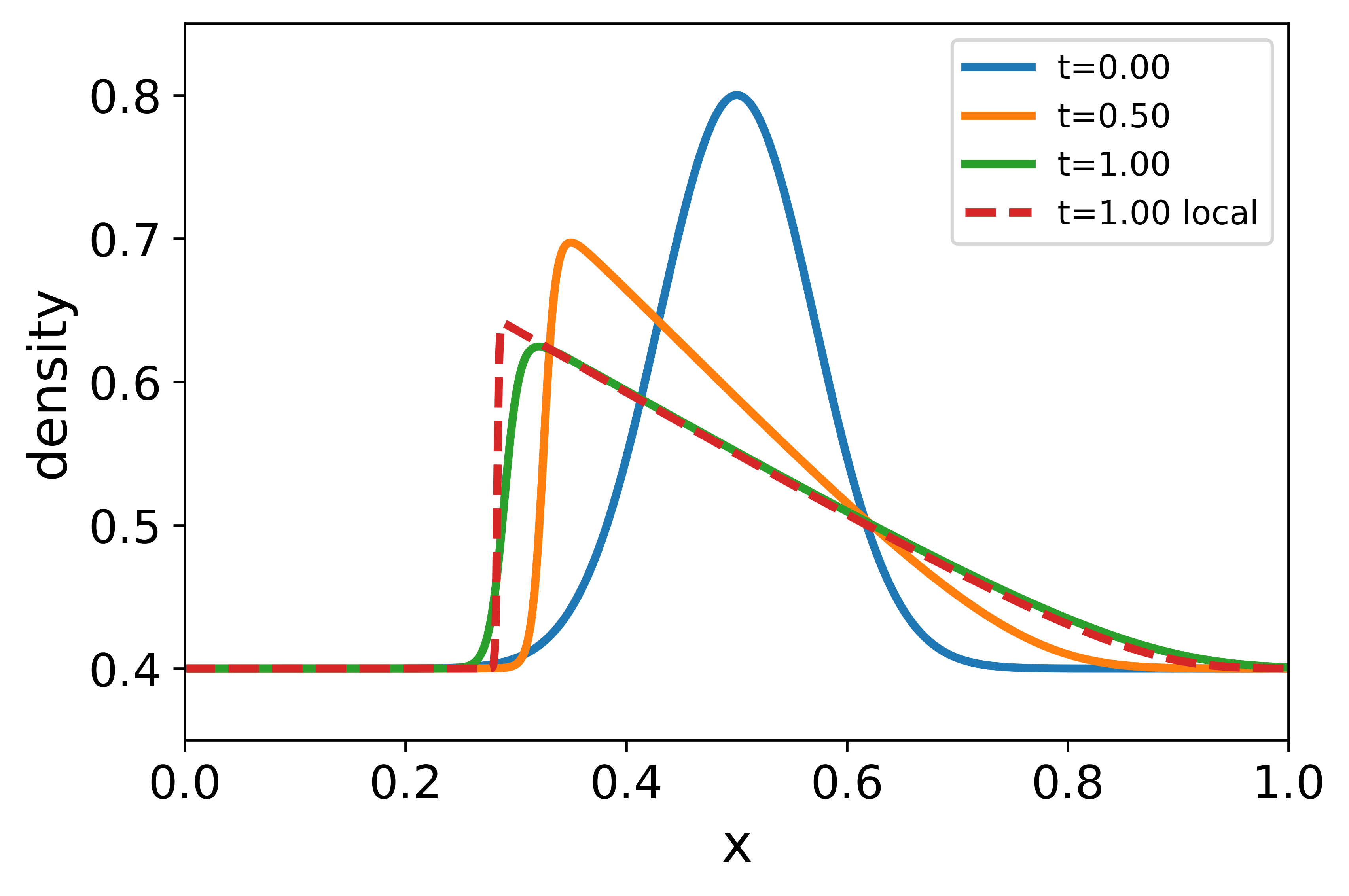
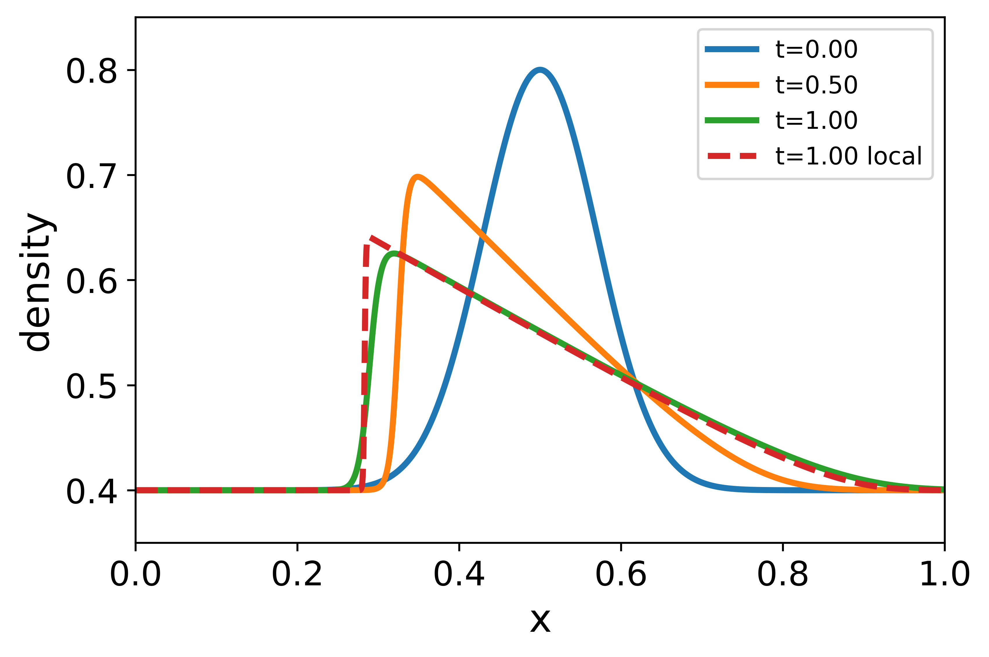
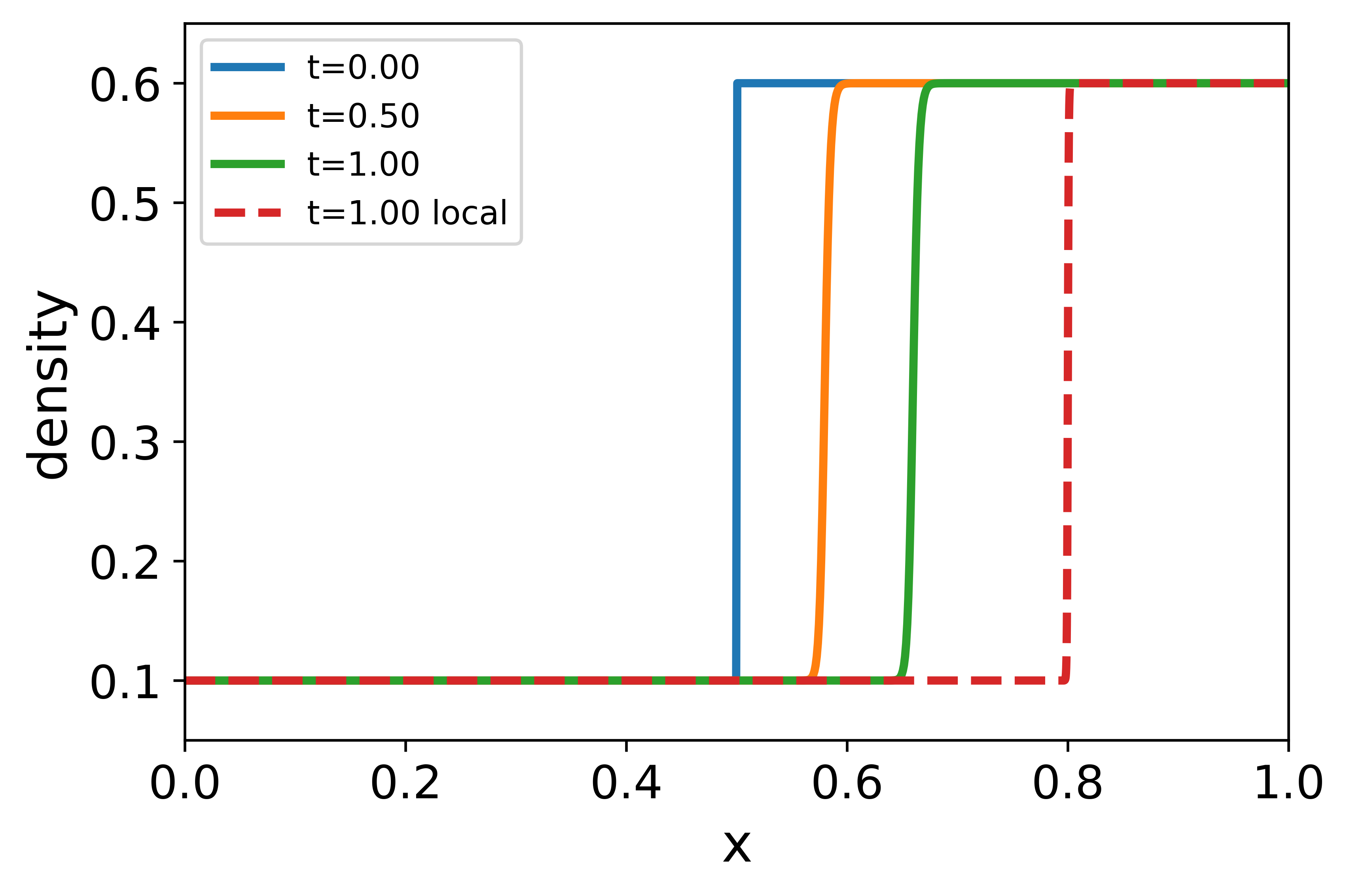
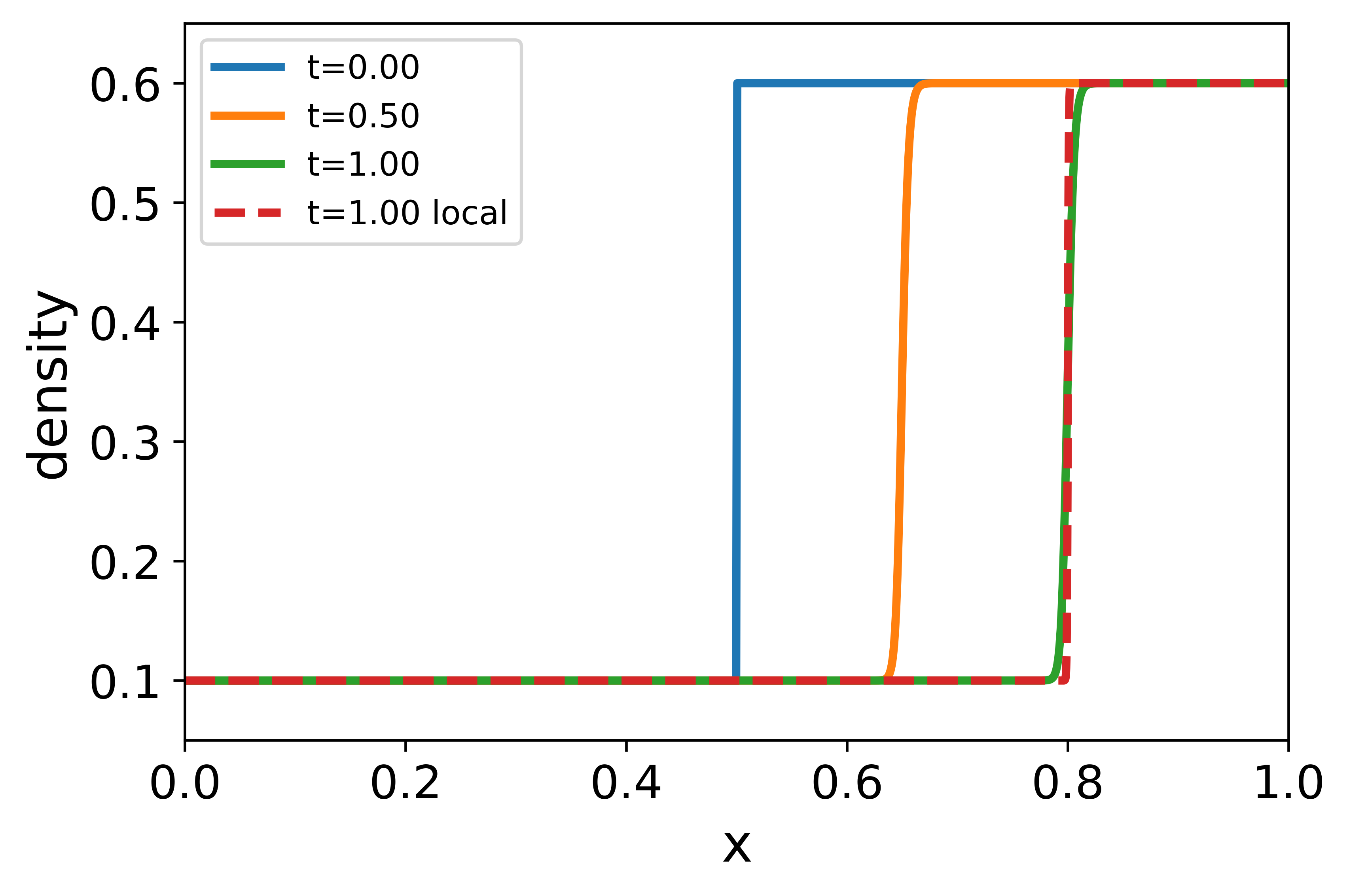
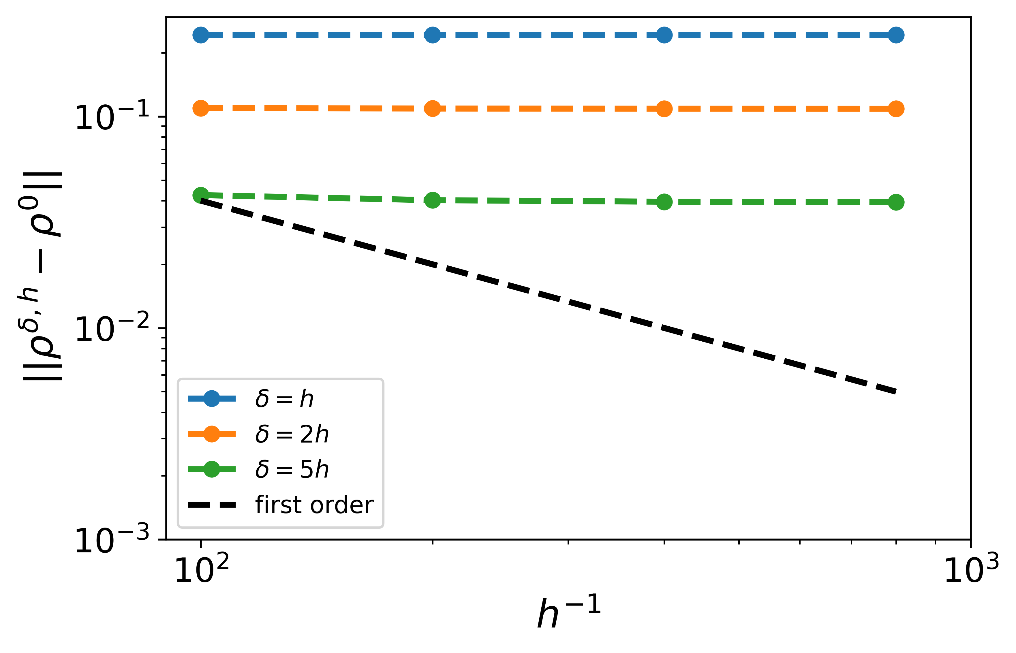
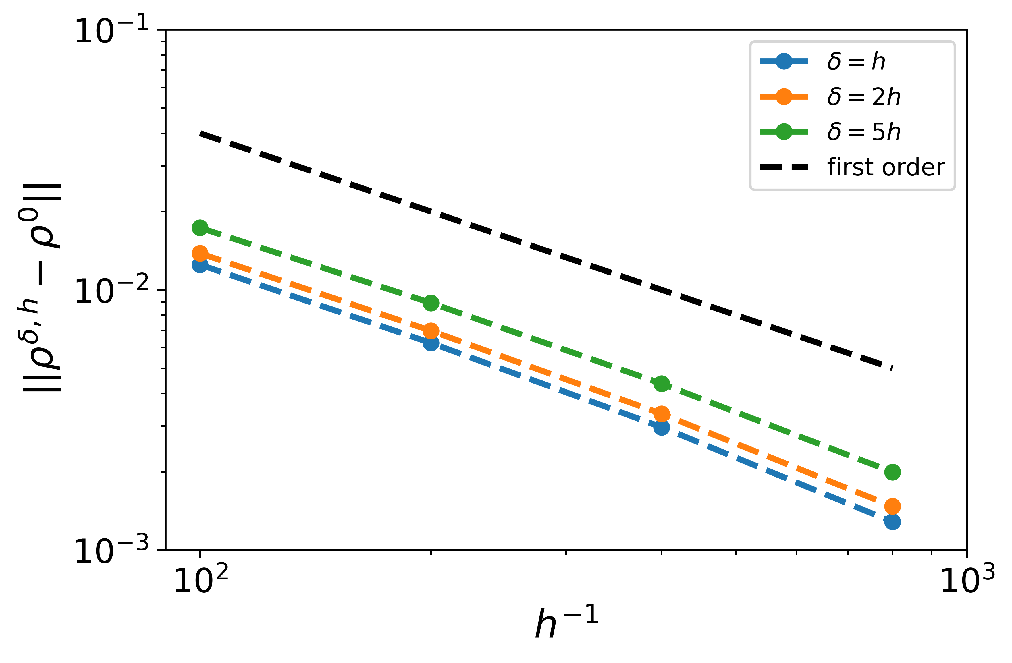
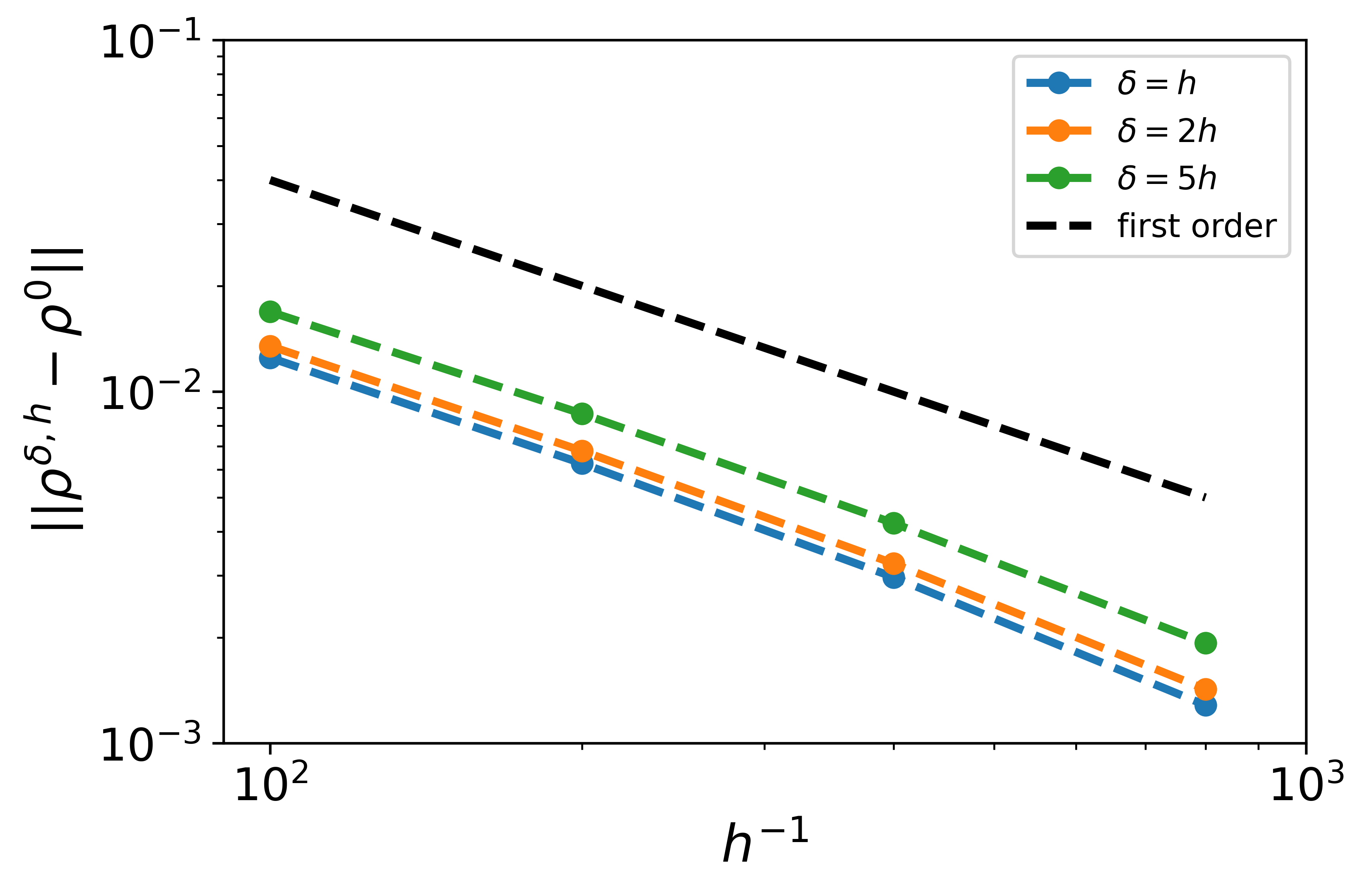
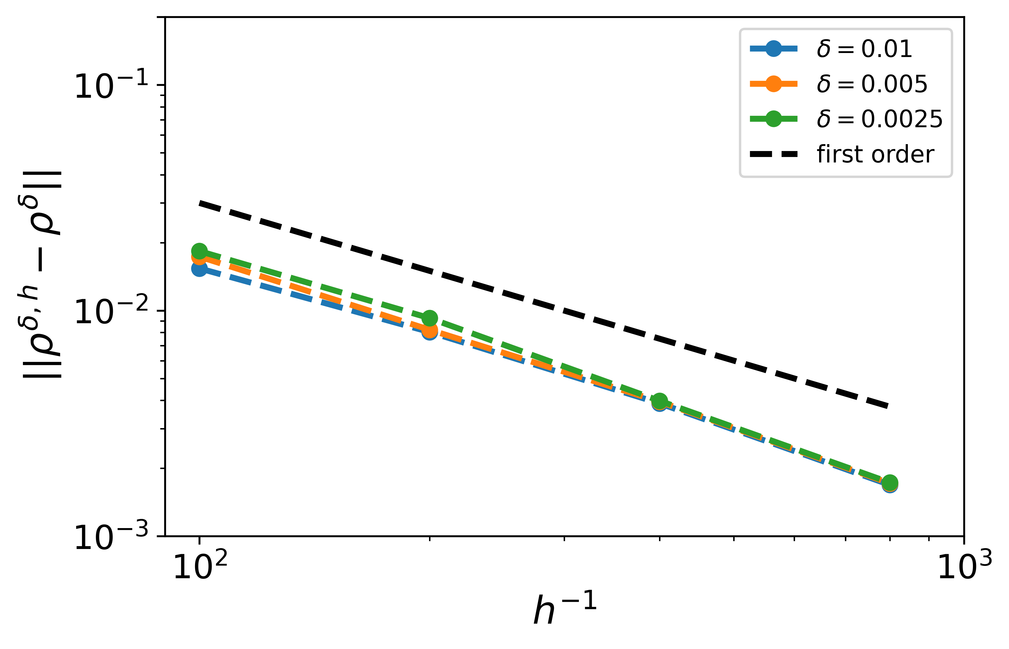
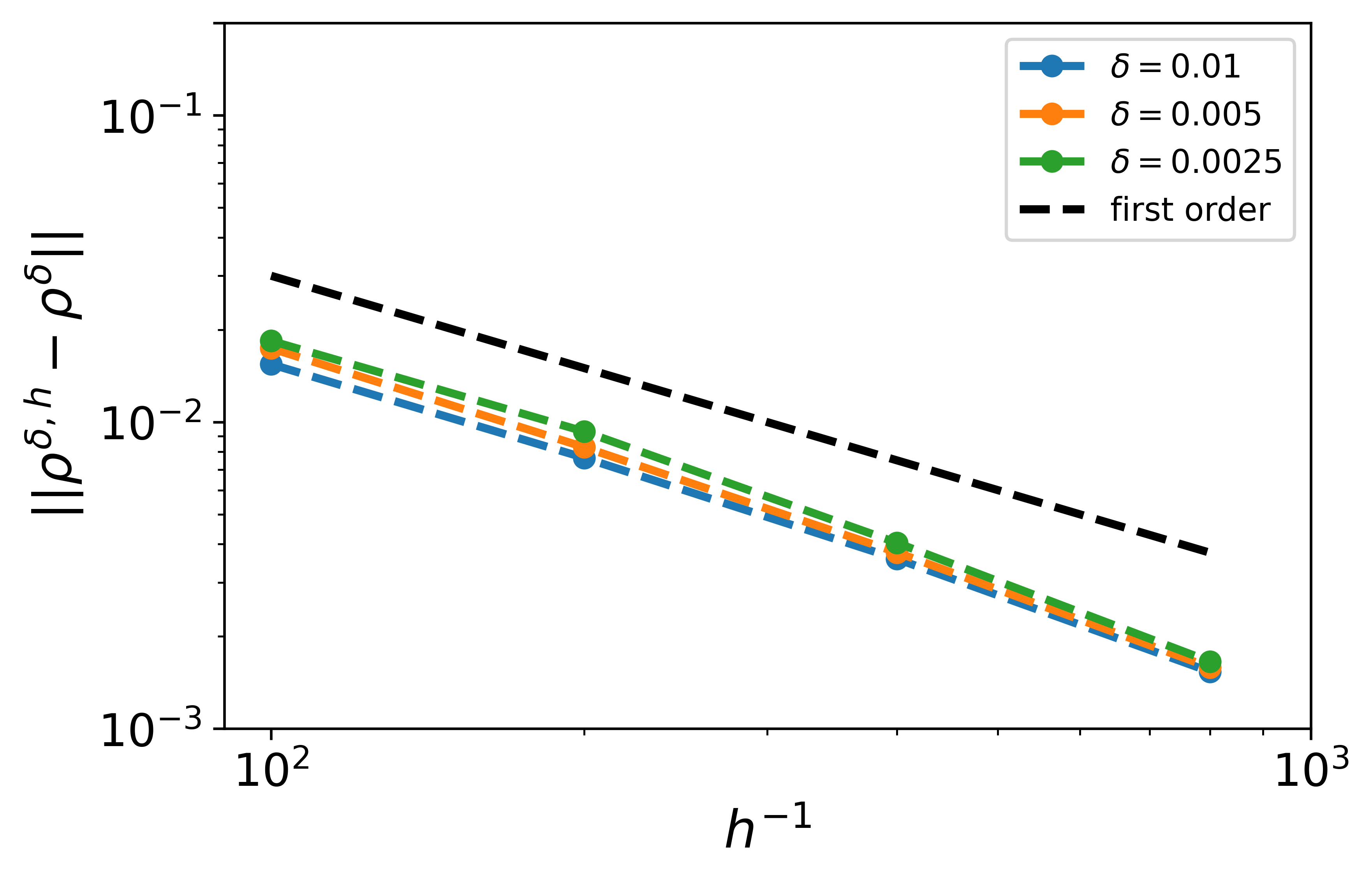
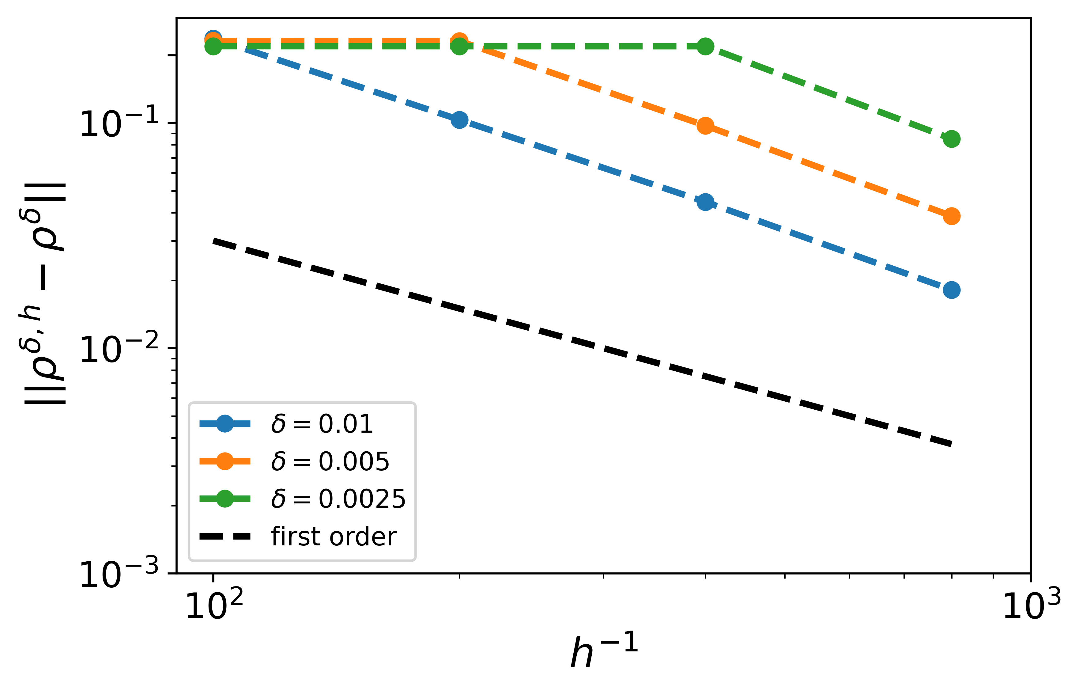
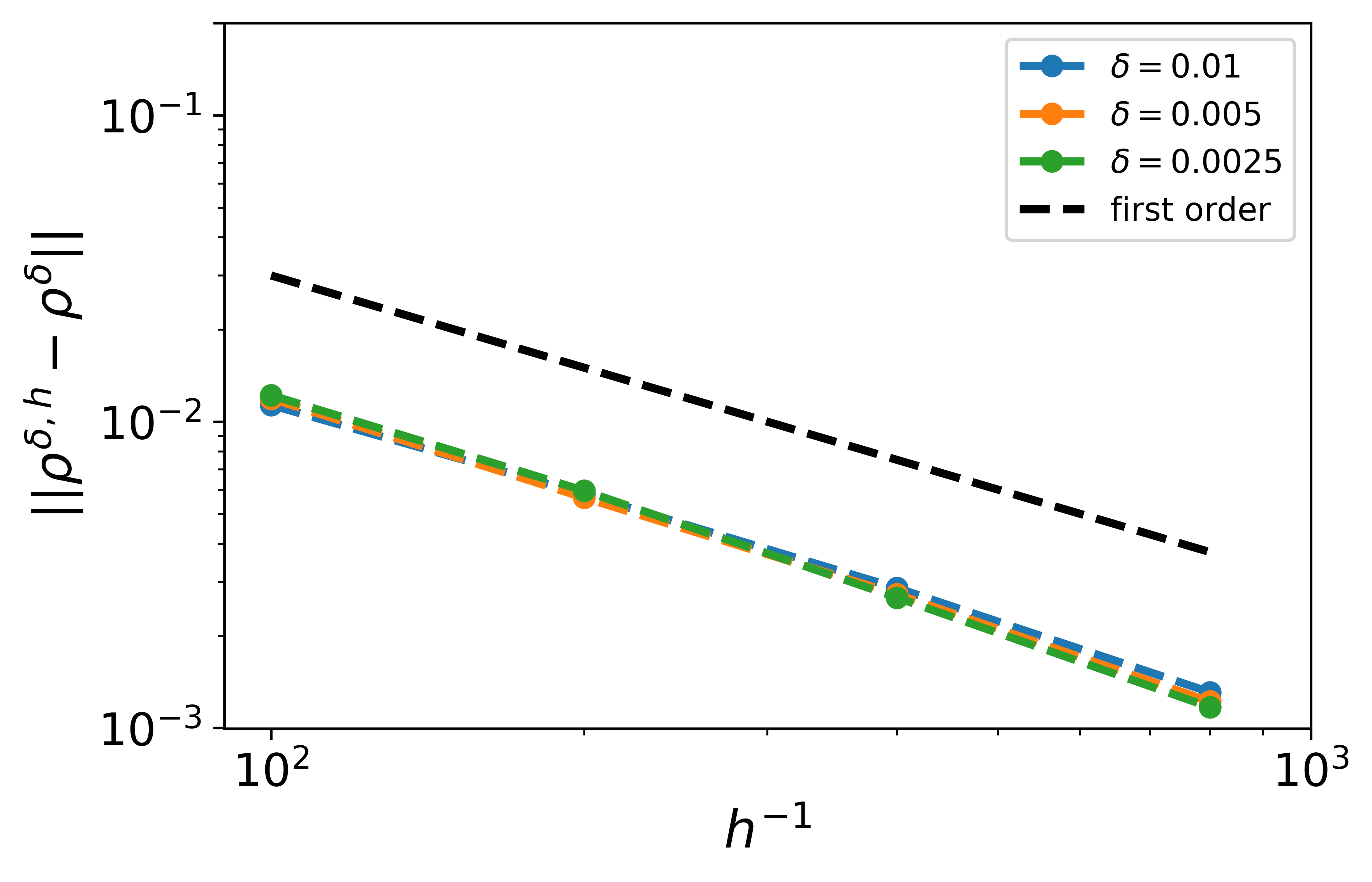
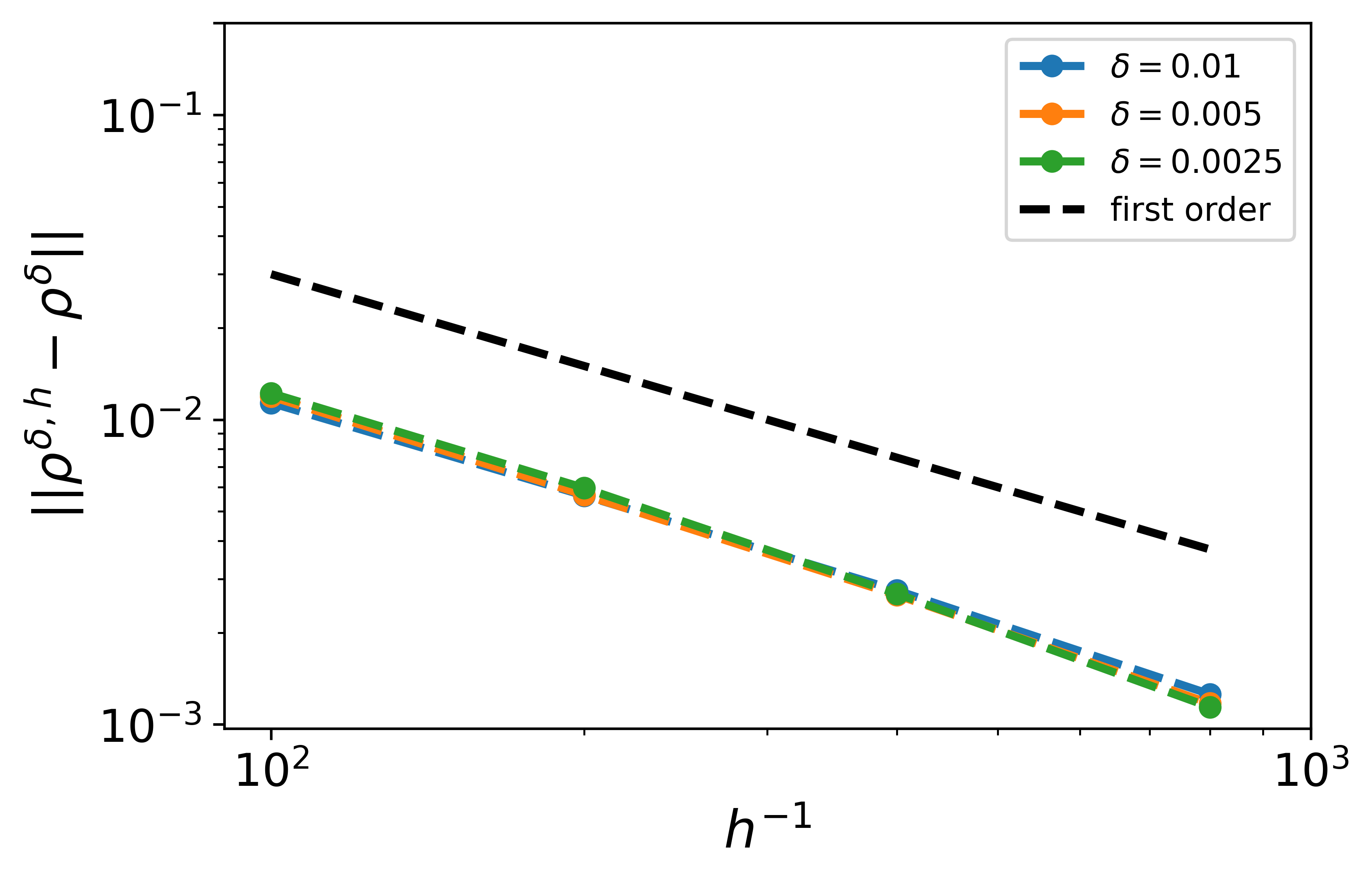
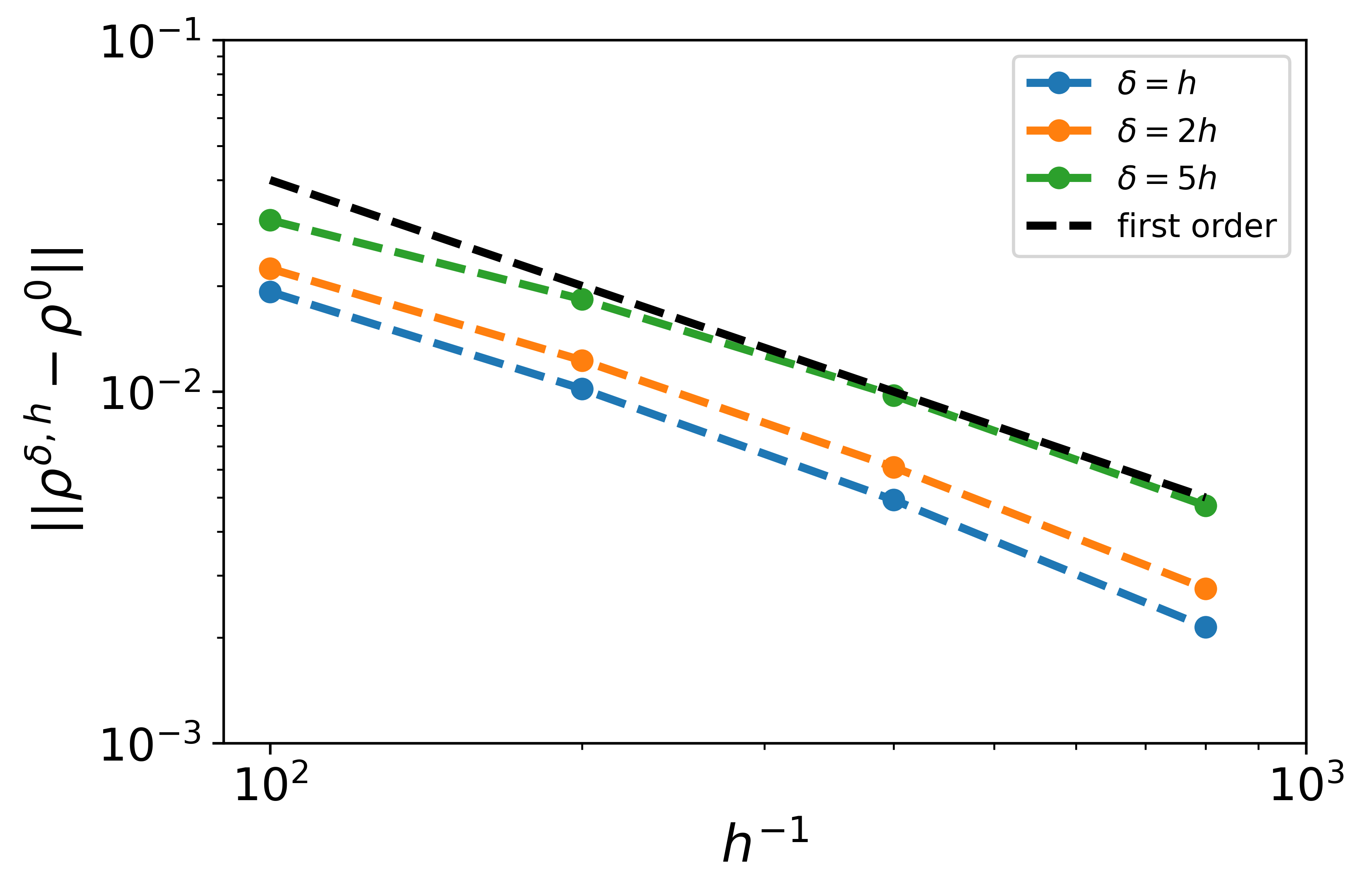
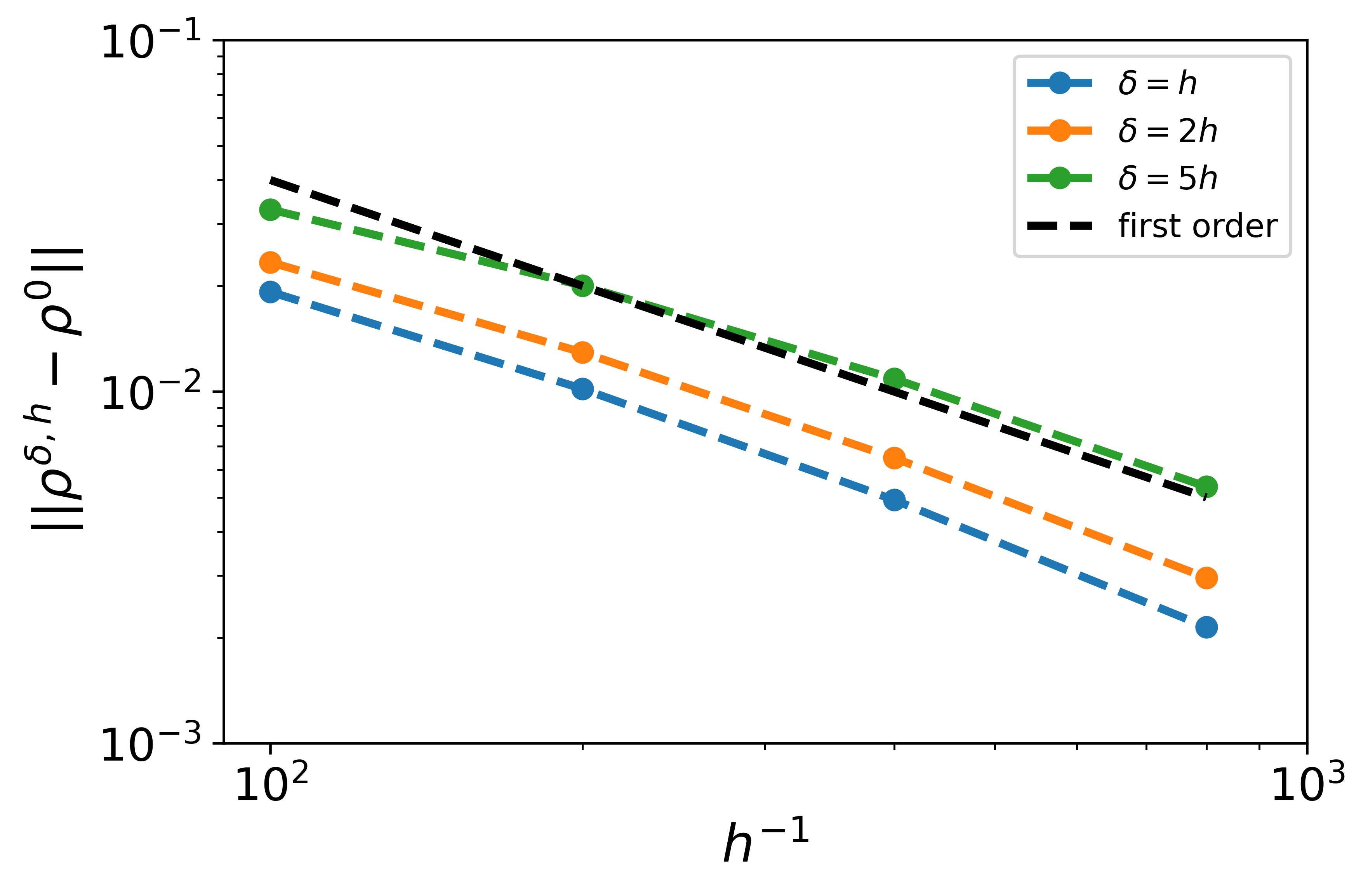
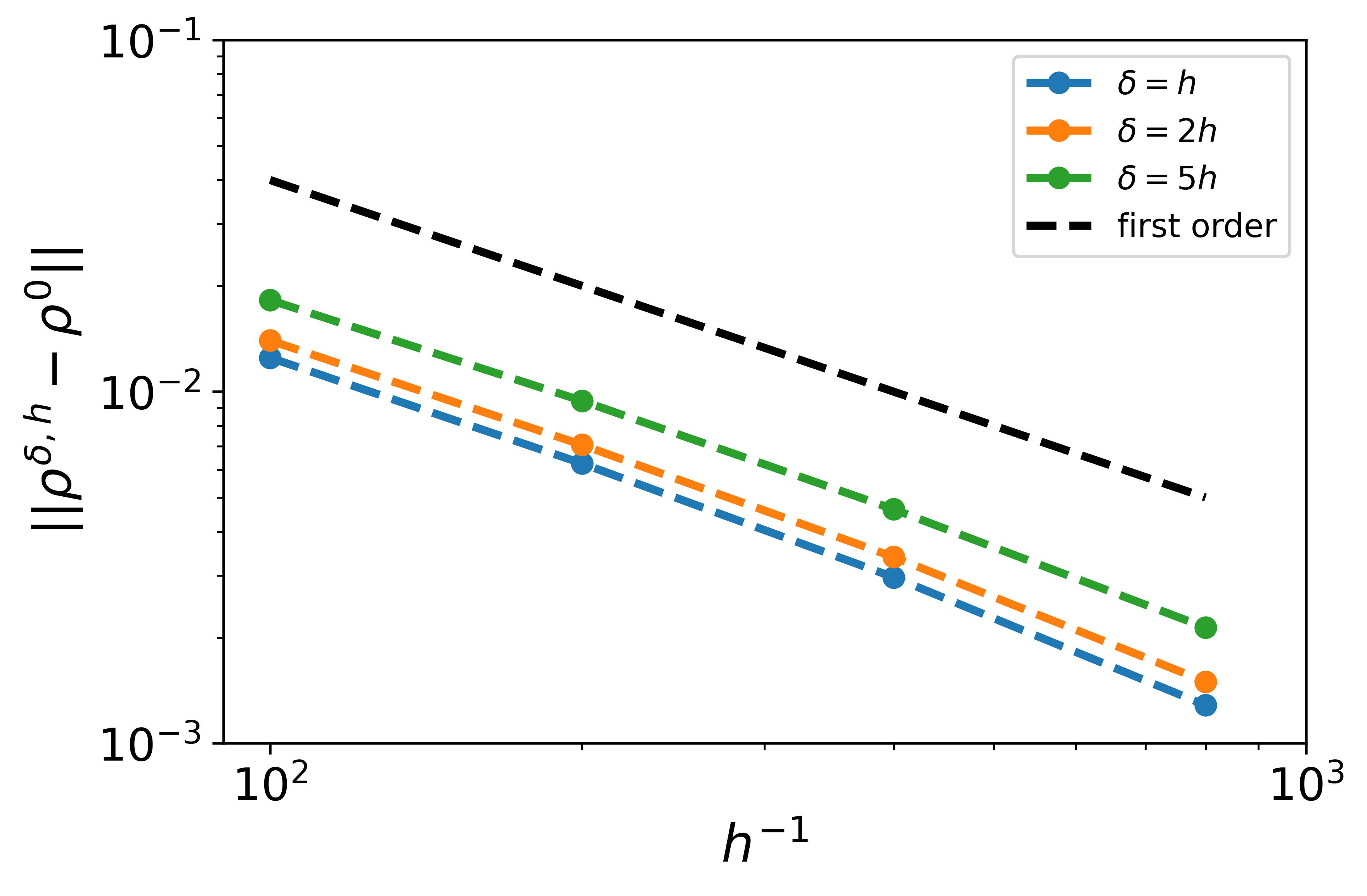
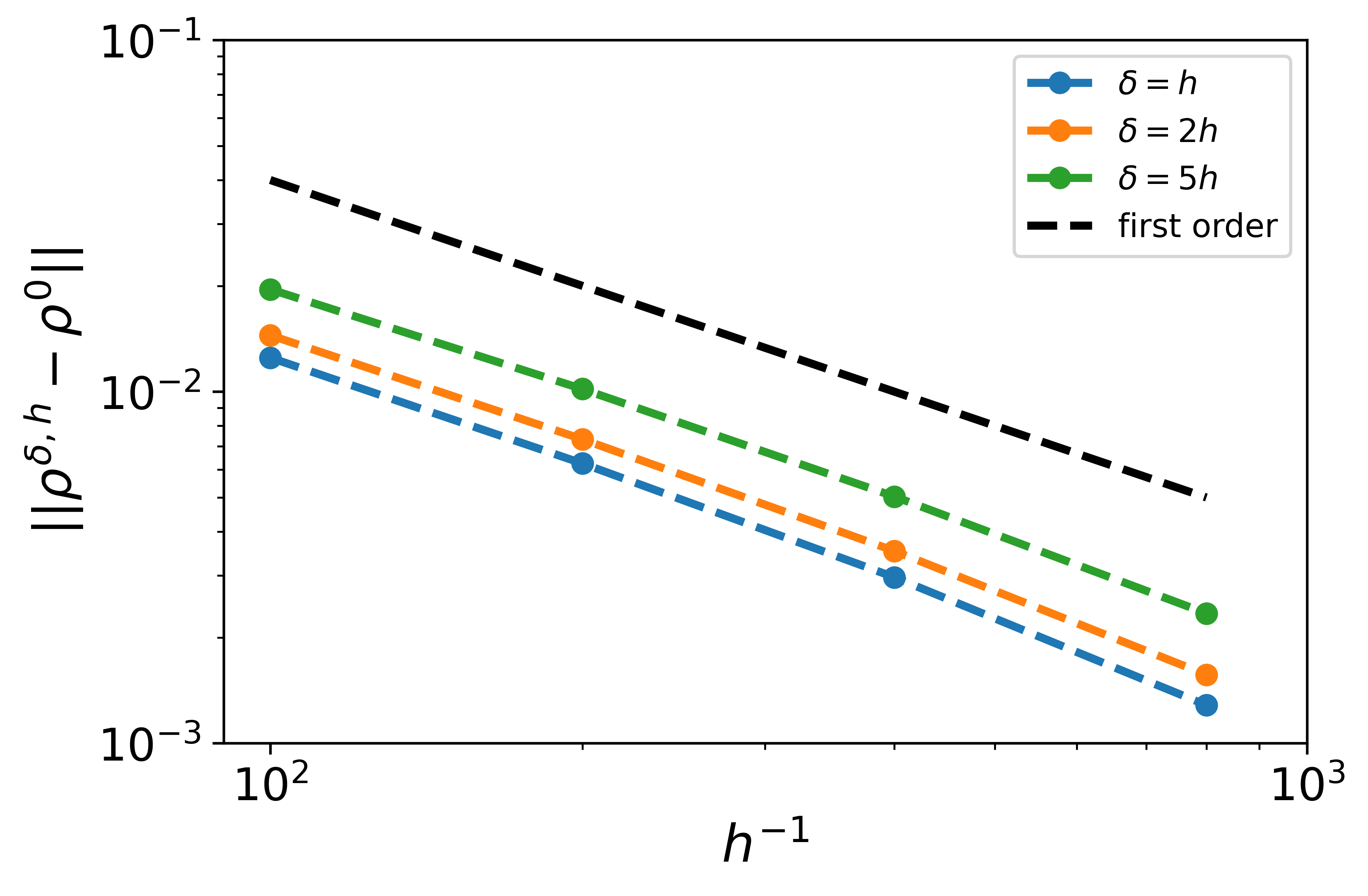
Let us make some remarks on the convergence rates in the above Theorem 2 and Theorem 3. On one hand, the scheme (21)-(22) is expected to be at most first order accurate because it is based on a piecewise constant approximation. On the other hand, for scalar conservation laws, it is known that a first order monotone scheme may have a O(h1/2)𝑂superscript12O(h^{1/2}) convergence rate for discontinuous solutions [35]. In the numerical experiments in Section 3, we test the scheme with both smooth initial data and discontinuous ones, the results validate the O(h)𝑂O(h) convergence rate to the local solution (as in Theorem 2) when δ=mh𝛿𝑚\delta=mh for a fixed integer m>0𝑚0m>0, and the O(h)𝑂O(h) convergence rate to the nonlocal solution uniformly in δ𝛿\delta (as in Theorem 3). We leave the rigorous analysis of convergence rates along various limiting paths in the future works.

Finally, we can also obtain the nonlocal-to-local limit of numerical discretizations, in particular, the following uniform convergence result.

Theorem 4.

Under Assumptions 1-5, for any h0>0subscript00h_{0}>0, we have

(37) limδ0suph(0,h0]ρδ,hρ0,h𝐋1(U)=0foranyboundedU[0,+)×.formulae-sequencesubscript𝛿0subscriptsupremum0subscript0subscriptdelimited-∥∥superscript𝜌𝛿superscript𝜌0superscript𝐋1𝑈0foranybounded𝑈0\displaystyle\lim_{\delta\to 0}\left.\sup_{h\in(0,h_{0}]}\left\lVert\rho^{\delta,h}-\rho^{0,h}\right\rVert_{\mathbf{L}^{1}(U)}\right.=0\quad\mathrm{for\ any\ bounded\ }U\subset[0,+\infty)\times\mathbb{R}.

1.4 Comments on numerical quadrature weights and numerical flux functions

Let us make some remarks on the choice of the numerical quadrature weights {wk}0km1subscriptsubscript𝑤𝑘0𝑘𝑚1\{w_{k}\}_{0\leq k\leq m-1}. Provided that the nonlocal kernel wδ=wδ(s)subscript𝑤𝛿subscript𝑤𝛿𝑠w_{\delta}=w_{\delta}(s) is 𝐂1superscript𝐂1\mathbf{C}^{1} smooth and decreasing, one can write the numerical quadrature weights as

wk=w(ξk)hδ,ξk[khδ,(k+1)hδ],k=0,,m1,formulae-sequencesubscript𝑤𝑘𝑤subscript𝜉𝑘𝛿formulae-sequencesubscript𝜉𝑘𝑘𝛿𝑘1𝛿𝑘0𝑚1\displaystyle w_{k}=w(\xi_{k})\frac{h}{\delta},\quad\xi_{k}\in\left[k\frac{h}{\delta},(k+1)\frac{h}{\delta}\right],\quad k=0,\cdots,m-1,

where {ξk}0km1subscriptsubscript𝜉𝑘0𝑘𝑚1\{\xi_{k}\}_{0\leq k\leq m-1} can be viewed as sampling points of a Riemann sum quadrature on [0,1]01[0,1].

The condition (25) in Assumption 3 basically requires that the sampling points should not be too close to each other, and the condition is used to derive the necessary a priori estimates on numerical solutions as in Theorem 1. To demonstrate the meaning of the constant c𝑐c and the factor m2superscript𝑚2m^{-2} in (25), let us illustrate with the left endpoint quadrature weights in (17). In this case,

wk1wk=hδ[w((k1)hδ)w(khδ)](mins[0,1]w(s))(hδ)2cm2,subscript𝑤𝑘1subscript𝑤𝑘𝛿delimited-[]𝑤𝑘1𝛿𝑤𝑘𝛿subscript𝑠01superscript𝑤𝑠superscript𝛿2𝑐superscript𝑚2\displaystyle w_{k-1}-w_{k}=\frac{h}{\delta}\left[w\left((k-1)\frac{h}{\delta}\right)-w\left(k\frac{h}{\delta}\right)\right]\geq\left(\min_{s\in[0,1]}-w^{\prime}(s)\right)\left(\frac{h}{\delta}\right)^{2}\geq cm^{-2},

where the constant c=mins[0,1]w(s)>0𝑐subscript𝑠01superscript𝑤𝑠0c=\min_{s\in[0,1]}-w^{\prime}(s)>0.

The condition (26) in Assumption 3 is the normalization condition for the numerical quadrature weights, which is essential to the consistency between the scheme (21)-(22) and the local model (1). To demonstrate potential risks when the normalization condition (26) is violated, let us consider the case δ=mh𝛿𝑚\delta=mh where m𝑚m is a fixed positive integer. Then the scheme (21)-(22) can be viewed as a m+2𝑚2m+2-point conservative scheme of the local model (1) with the numerical flux function:

glocal(ρj,,ρj+m)=g(ρj,ρj+1,k=0m1wkρj+k,k=0m1wkρj+k+1),subscript𝑔localsubscript𝜌𝑗subscript𝜌𝑗𝑚𝑔subscript𝜌𝑗subscript𝜌𝑗1superscriptsubscript𝑘0𝑚1subscript𝑤𝑘subscript𝜌𝑗𝑘superscriptsubscript𝑘0𝑚1subscript𝑤𝑘subscript𝜌𝑗𝑘1\displaystyle g_{\mathrm{local}}(\rho_{j},\cdots,\rho_{j+m})=g\left(\rho_{j},\rho_{j+1},\sum_{k=0}^{m-1}w_{k}\rho_{j+k},\sum_{k=0}^{m-1}w_{k}\rho_{j+k+1}\right),

where g𝑔g is as in Assumption 4. Suppose ρj==ρj+m=ρ¯subscript𝜌𝑗subscript𝜌𝑗𝑚¯𝜌\rho_{j}=\cdots=\rho_{j+m}=\bar{\rho}, to make glocalsubscript𝑔localg_{\mathrm{local}} consistent to the local model (1), it is necessary to have

glocal(ρ¯,,ρ¯)=ρ¯(1ρ¯k=0m1wk)=ρ¯(1ρ¯),subscript𝑔local¯𝜌¯𝜌¯𝜌1¯𝜌superscriptsubscript𝑘0𝑚1subscript𝑤𝑘¯𝜌1¯𝜌\displaystyle g_{\mathrm{local}}(\bar{\rho},\cdots,\bar{\rho})=\bar{\rho}\left(1-\bar{\rho}\sum_{k=0}^{m-1}w_{k}\right)=\bar{\rho}(1-\bar{\rho}),

which requires the normalization condition (26). In contrast, if the condition (26) is violated and ηk=0m1wk1approaches-limit𝜂superscriptsubscript𝑘0𝑚1subscript𝑤𝑘1\eta\doteq\sum_{k=0}^{m-1}w_{k}\neq 1, the numerical solutions will formally converge to a solution of the equation

tρ(t,x)+x(ρ(t,x)(1ηρ(t,x)))=0,subscript𝑡𝜌𝑡𝑥subscript𝑥𝜌𝑡𝑥1𝜂𝜌𝑡𝑥0\displaystyle\partial_{t}\rho(t,x)+\partial_{x}(\rho(t,x)(1-\eta\rho(t,x)))=0,

other than the desired equation (1) with v(ρ)=1ρ𝑣𝜌1𝜌v(\rho)=1-\rho. This means that the absence of the normalization condition (26) for some numerical quadrature weights may lead to incorrect limit solutions when δ0𝛿0\delta\to 0 and h00h\to 0 simultaneously. Hence, we introduce the following normalized left endpoint quadrature weights:

(38) [Normalized left endpoint]wk=wδ(kh)hk=0m1wδ(kh)h,k=0,,m1,formulae-sequence[Normalized left endpoint]subscript𝑤𝑘subscript𝑤𝛿𝑘superscriptsubscript𝑘0𝑚1subscript𝑤𝛿𝑘𝑘0𝑚1\displaystyle\mbox{[Normalized left endpoint]}\quad w_{k}=\frac{w_{\delta}(kh)h}{\sum_{k=0}^{m-1}w_{\delta}(kh)h},\quad k=0,\cdots,m-1,

and give the following proposition.

Proposition 3.

The normalized left endpoint quadrature weights (38) and the exact quadrature weights (19) both satisfy the Assumption 3, with the constant c𝑐c in the condition (25) given by c=11+w(0)mins[0,1]w(s)𝑐11𝑤0subscript𝑠01superscript𝑤𝑠c=\frac{1}{1+w(0)}\min_{s\in[0,1]}-w^{\prime}(s) and c=mins[0,1]w(s)𝑐subscript𝑠01superscript𝑤𝑠c=\min_{s\in[0,1]}-w^{\prime}(s), respectively. The left endpoint quadrature weights satisfy the condition (25) with the constant c=mins[0,1]w(s)𝑐subscript𝑠01superscript𝑤𝑠c=\min_{s\in[0,1]}-w^{\prime}(s) but they do not satisfy the normalization condition (26).

A comparison between the different choices of numerical quadrature weights is made through numerical experiments in Section 3.

Concerning the Assumption 4 on the numerical flux function g𝑔g, with the velocity function v(ρ)=1ρ𝑣𝜌1𝜌v(\rho)=1-\rho, the flux function in the continuum model (2) is ρ(1q)𝜌1𝑞\rho(1-q), which is a quadratic polynomial of (ρ,q)𝜌𝑞(\rho,q) with the only quadratic term being ρq𝜌𝑞-\rho q. It is then reasonable to assume that the numerical flux function g𝑔g is quadratic with its second order derivatives satisfying the condition (iii). The condition (ii) guarantees the consistency of the scheme (21)-(22) to the model (2). The condition (iv) is used to show that the scheme is monotone under all Assumptions 1-5, see the Theorem 1. It is natural to ask if the results in this work can be extended to more general numerical flux functions, e.g., g𝑔g is not quadratic. We leave the study of such an extension to future works.

Let us mention that the numerical flux functions given in (24a)-(24c) all satisfy Assumption 4. For the two Lax-Friedrichs type numerical flux functions (24a) and (24c), the numerical viscosity constant should satisfy α2𝛼2\alpha\geq 2.

We also remark that, in the case of 0<δh0𝛿0<\delta\leq h, i.e., the nonlocal horizon is within one spatial mesh cell, it holds that qL=ρLsubscript𝑞𝐿subscript𝜌𝐿q_{L}=\rho_{L} and qR=ρRsubscript𝑞𝑅subscript𝜌𝑅q_{R}=\rho_{R} by Assumption 3. Suppose g𝑔g satisfies Assumption 4, the numerical flux function g=g(ρL,ρR,ρL,ρR)𝑔𝑔subscript𝜌𝐿subscript𝜌𝑅subscript𝜌𝐿subscript𝜌𝑅g=g(\rho_{L},\rho_{R},\rho_{L},\rho_{R}) for the local model (1) is non-decreasing with respect to ρLsubscript𝜌𝐿\rho_{L} and non-increasing with respect to ρRsubscript𝜌𝑅\rho_{R}. Therefore, the scheme (23) is a monotone scheme for the local model (1). As a consequence, we give the following result.

Proposition 4.

Under Assumptions 1, 3-5, let ρδ,hsuperscript𝜌𝛿\rho^{\delta,h} be the numerical solution produced by the scheme (21)-(22) and ρ0,hsuperscript𝜌0\rho^{0,h} be the one produced by (23). It holds that:

ρδ,h=ρ0,hwhen0<δh.formulae-sequencesuperscript𝜌𝛿superscript𝜌0when0𝛿\displaystyle\rho^{\delta,h}=\rho^{0,h}\quad\mathrm{when}\quad 0<\delta\leq h.

Moreover, ρ0,hsuperscript𝜌0\rho^{0,h} converges in 𝐋loc1([0,+)×)subscriptsuperscript𝐋1loc0\mathbf{L}^{1}_{\mathrm{loc}}([0,+\infty)\times\mathbb{R}) to the weak entropy solution ρ0superscript𝜌0\rho^{0} of the local model (1) as defined in Proposition 2.

2 Proof of theorems

This section aims to give the proofs of our main results. First, in Section 2.1, we show the maximum principle for numerical solutions. Then we present an one-sided Lipschitz estimate for numerical solutions in Section 2.2, the monotonicity of the numerical scheme (21)-(22) and the total variation estimate for numerical solutions follow as corollaries. These two subsections constitute the proof of Theorem 1. In Section 2.3, we let h00h\to 0 and show convergence of numerical solutions to the proper nonlocal or local solution, which gives the proofs of Theorem 2 and Theorem 3. In Section 2.4, we give the proof of Theorem 4 on the nonlocal-to-local limit of numerical discretizations.

2.1 Maximum principle

In this subsection, we aim to show the maximum principle (34) in Theorem 1. By Assumption 1 and (12), the numerical solution at the initial time {ρj0}jsubscriptsuperscriptsubscript𝜌𝑗0𝑗\{\rho_{j}^{0}\}_{j\in\mathbb{Z}} satisfies 0ρj010superscriptsubscript𝜌𝑗010\leq\rho_{j}^{0}\leq 1 for all j𝑗{j\in\mathbb{Z}}. Then the maximum principle (34) can be proved by induction using the following Lemma 4.1.

Lemma 4.1.

Suppose all conditions in Theorem 1 are given, and that 0ρminρj+knρmax10subscript𝜌minsuperscriptsubscript𝜌𝑗𝑘𝑛subscript𝜌max10\leq\rho_{\mathrm{min}}\leq\rho_{j+k}^{n}\leq\rho_{\mathrm{max}}\leq 1 for k=1,0,1,,m𝑘101𝑚k=-1,0,1,\cdots,m. Then we have

(39) ρmin(ρj1n,ρjn,ρj+1n,,ρj+mn)ρmax,subscript𝜌minsubscriptsuperscript𝜌𝑛𝑗1subscriptsuperscript𝜌𝑛𝑗subscriptsuperscript𝜌𝑛𝑗1subscriptsuperscript𝜌𝑛𝑗𝑚subscript𝜌max\displaystyle\rho_{\mathrm{min}}\leq\mathcal{H}(\rho^{n}_{j-1},\rho^{n}_{j},\rho^{n}_{j+1},\cdots,\rho^{n}_{j+m})\leq\rho_{\mathrm{max}},

where the operator \mathcal{H} is as defined in (21)-(22).

Let us first check the monotonicity of the scheme defined by (21)-(22). Denote

θjn,(i)=θ(i)(qj1n,qjn),i=1,2;θjn,(i)=θ(i)(ρj1n,ρjn),i=3,4forj,n0.formulae-sequencesuperscriptsubscript𝜃𝑗𝑛𝑖superscript𝜃𝑖superscriptsubscript𝑞𝑗1𝑛superscriptsubscript𝑞𝑗𝑛formulae-sequence𝑖12formulae-sequencesuperscriptsubscript𝜃𝑗𝑛𝑖superscript𝜃𝑖superscriptsubscript𝜌𝑗1𝑛superscriptsubscript𝜌𝑗𝑛formulae-sequence𝑖34forformulae-sequence𝑗𝑛0\displaystyle\theta_{j}^{n,(i)}=\theta^{(i)}(q_{j-1}^{n},q_{j}^{n}),\ i=1,2;\quad\theta_{j}^{n,(i)}=\theta^{(i)}(\rho_{j-1}^{n},\rho_{j}^{n}),\ i=3,4\quad\text{for}\quad j\in\mathbb{Z},\ n\geq 0.

A direct calculation gives:

(40a) ρj1nsubscriptsuperscript𝜌𝑛𝑗1\displaystyle\frac{\partial\mathcal{H}}{\partial\rho^{n}_{j-1}} =λ(θjn,(1)+w0θjn,(3));absent𝜆superscriptsubscript𝜃𝑗𝑛1subscript𝑤0superscriptsubscript𝜃𝑗𝑛3\displaystyle=\lambda\left(\theta_{j}^{n,(1)}+w_{0}\theta_{j}^{n,(3)}\right);
(40b) ρjnsubscriptsuperscript𝜌𝑛𝑗\displaystyle\frac{\partial\mathcal{H}}{\partial\rho^{n}_{j}} =1+λ(θjn,(2)θj+1n,(1)+w1θjn,(3)+w0θjn,(4)w0θj+1n,(3));absent1𝜆superscriptsubscript𝜃𝑗𝑛2superscriptsubscript𝜃𝑗1𝑛1subscript𝑤1superscriptsubscript𝜃𝑗𝑛3subscript𝑤0superscriptsubscript𝜃𝑗𝑛4subscript𝑤0superscriptsubscript𝜃𝑗1𝑛3\displaystyle=1+\lambda\left(\theta_{j}^{n,(2)}-\theta_{j+1}^{n,(1)}+w_{1}\theta_{j}^{n,(3)}+w_{0}\theta_{j}^{n,(4)}-w_{0}\theta_{j+1}^{n,(3)}\right);
(40c) ρj+1nsubscriptsuperscript𝜌𝑛𝑗1\displaystyle\frac{\partial\mathcal{H}}{\partial\rho^{n}_{j+1}} =λ(w2θjn,(3)+w1θjn,(4)θj+1n,(2)w1θj+1n,(3)w0θj+1n,(4));absent𝜆subscript𝑤2superscriptsubscript𝜃𝑗𝑛3subscript𝑤1superscriptsubscript𝜃𝑗𝑛4superscriptsubscript𝜃𝑗1𝑛2subscript𝑤1superscriptsubscript𝜃𝑗1𝑛3subscript𝑤0superscriptsubscript𝜃𝑗1𝑛4\displaystyle=\lambda\left(w_{2}\theta_{j}^{n,(3)}+w_{1}\theta_{j}^{n,(4)}-\theta_{j+1}^{n,(2)}-w_{1}\theta_{j+1}^{n,(3)}-w_{0}\theta_{j+1}^{n,(4)}\right);
(40d) ρj+knsubscriptsuperscript𝜌𝑛𝑗𝑘\displaystyle\frac{\partial\mathcal{H}}{\partial\rho^{n}_{j+k}} =λ(wk+1θjn,(3)wkθj+1n,(3)+wkθjn,(4)wk1θj+1n,(4)),k=2,,m;formulae-sequenceabsent𝜆subscript𝑤𝑘1superscriptsubscript𝜃𝑗𝑛3subscript𝑤𝑘superscriptsubscript𝜃𝑗1𝑛3subscript𝑤𝑘superscriptsubscript𝜃𝑗𝑛4subscript𝑤𝑘1superscriptsubscript𝜃𝑗1𝑛4𝑘2𝑚\displaystyle=\lambda\left(w_{k+1}\theta_{j}^{n,(3)}-w_{k}\theta_{j+1}^{n,(3)}+w_{k}\theta_{j}^{n,(4)}-w_{k-1}\theta_{j+1}^{n,(4)}\right),\quad k=2,\cdots,m;

where we make the convention that wm=wm+1=0subscript𝑤𝑚subscript𝑤𝑚10w_{m}=w_{m+1}=0.

In (40d) that corresponds to the nonlocal dependence of the flux on the solution, it is possible that θjn,(3)<0,θjn,(4)<0formulae-sequencesuperscriptsubscript𝜃𝑗𝑛30superscriptsubscript𝜃𝑗𝑛40\theta_{j}^{n,(3)}<0,\,\theta_{j}^{n,(4)}<0 while θj+1n,(3)=θj+1n,(4)=0superscriptsubscript𝜃𝑗1𝑛3superscriptsubscript𝜃𝑗1𝑛40\theta_{j+1}^{n,(3)}=\theta_{j+1}^{n,(4)}=0 at some point j=j0𝑗subscript𝑗0j=j_{0}, e.g., if we consider the Riemann type solution:

ρjn=1,jj0;ρjn=0,j>j0.formulae-sequencesuperscriptsubscript𝜌𝑗𝑛1formulae-sequence𝑗subscript𝑗0formulae-sequencesuperscriptsubscript𝜌𝑗𝑛0𝑗subscript𝑗0\displaystyle\rho_{j}^{n}=1,\ j\leq j_{0};\quad\rho_{j}^{n}=0,\ j>j_{0}.

In this case, ρj+kn<0subscriptsuperscript𝜌𝑛𝑗𝑘0\frac{\partial\mathcal{H}}{\partial\rho^{n}_{j+k}}<0 for k=2,,m1𝑘2𝑚1k=2,\cdots,m-1. Therefore, one can not deduce (39) by showing (21)-(22) is a monotone scheme. Here we prove (39) in an alternative way, which was also used in [26, 24].

Proof of Lemma 4.1.

We observe the identity (ρmin,ρmin,ρmin,,ρmin)=ρminsubscript𝜌minsubscript𝜌minsubscript𝜌minsubscript𝜌minsubscript𝜌min\mathcal{H}(\rho_{\mathrm{min}},\rho_{\mathrm{min}},\rho_{\mathrm{min}},\cdots,\rho_{\mathrm{min}})=\rho_{\mathrm{min}} thus we can write the term (ρj1n,ρjn,ρj+1n,,ρj+mn)ρminsubscriptsuperscript𝜌𝑛𝑗1subscriptsuperscript𝜌𝑛𝑗subscriptsuperscript𝜌𝑛𝑗1subscriptsuperscript𝜌𝑛𝑗𝑚subscript𝜌min\mathcal{H}(\rho^{n}_{j-1},\rho^{n}_{j},\rho^{n}_{j+1},\cdots,\rho^{n}_{j+m})-\rho_{\mathrm{min}} as the summation of two parts:

Δ1=Δsubscript1absent\displaystyle\Delta\mathcal{H}_{1}= (ρj1n,ρjn,ρj+1n,ρj+2n,ρj+mn)(ρmin,ρmin,ρj+1n,ρj+2n,,ρj+mn),subscriptsuperscript𝜌𝑛𝑗1subscriptsuperscript𝜌𝑛𝑗subscriptsuperscript𝜌𝑛𝑗1subscriptsuperscript𝜌𝑛𝑗2subscriptsuperscript𝜌𝑛𝑗𝑚subscript𝜌minsubscript𝜌minsubscriptsuperscript𝜌𝑛𝑗1subscriptsuperscript𝜌𝑛𝑗2subscriptsuperscript𝜌𝑛𝑗𝑚\displaystyle\mathcal{H}(\rho^{n}_{j-1},\rho^{n}_{j},\rho^{n}_{j+1},\rho^{n}_{j+2}\cdots,\rho^{n}_{j+m})-\mathcal{H}(\rho_{\mathrm{min}},\rho_{\mathrm{min}},\rho^{n}_{j+1},\rho^{n}_{j+2},\cdots,\rho^{n}_{j+m}),
Δ2=Δsubscript2absent\displaystyle\Delta\mathcal{H}_{2}= (ρmin,ρmin,ρj+1n,ρj+2n,,ρj+mn)(ρmin,ρmin,ρmin,ρmin,ρmin).subscript𝜌minsubscript𝜌minsubscriptsuperscript𝜌𝑛𝑗1subscriptsuperscript𝜌𝑛𝑗2subscriptsuperscript𝜌𝑛𝑗𝑚subscript𝜌minsubscript𝜌minsubscript𝜌minsubscript𝜌minsubscript𝜌min\displaystyle\mathcal{H}(\rho_{\mathrm{min}},\rho_{\mathrm{min}},\rho^{n}_{j+1},\rho^{n}_{j+2},\cdots,\rho^{n}_{j+m})-\mathcal{H}(\rho_{\mathrm{min}},\rho_{\mathrm{min}},\rho_{\mathrm{min}},\rho_{\mathrm{min}}\cdots,\rho_{\mathrm{min}}).

By the mean value theorem,

Δ1Δsubscript1\displaystyle\Delta\mathcal{H}_{1} =k=1,0ρj+kn(ρ~j1n,ρ~jn,ρj+1n,ρj+2n,ρj+mn)(ρj+knρmin),absentsubscript𝑘10subscriptsuperscript𝜌𝑛𝑗𝑘subscriptsuperscript~𝜌𝑛𝑗1subscriptsuperscript~𝜌𝑛𝑗subscriptsuperscript𝜌𝑛𝑗1subscriptsuperscript𝜌𝑛𝑗2subscriptsuperscript𝜌𝑛𝑗𝑚subscriptsuperscript𝜌𝑛𝑗𝑘subscript𝜌min\displaystyle=\sum_{k=-1,0}\frac{\partial\mathcal{H}}{\partial\rho^{n}_{j+k}}(\tilde{\rho}^{n}_{j-1},\tilde{\rho}^{n}_{j},\rho^{n}_{j+1},\rho^{n}_{j+2}\cdots,\rho^{n}_{j+m})(\rho^{n}_{j+k}-\rho_{\mathrm{min}}),
Δ2Δsubscript2\displaystyle\Delta\mathcal{H}_{2} =1kmρj+kn(ρmin,ρmin,ρ~j+1n,ρ~j+2n,ρ~j+mn)(ρj+knρmin),absentsubscript1𝑘𝑚subscriptsuperscript𝜌𝑛𝑗𝑘subscript𝜌minsubscript𝜌minsubscriptsuperscript~𝜌𝑛𝑗1subscriptsuperscript~𝜌𝑛𝑗2subscriptsuperscript~𝜌𝑛𝑗𝑚subscriptsuperscript𝜌𝑛𝑗𝑘subscript𝜌min\displaystyle=\sum_{1\leq k\leq m}\frac{\partial\mathcal{H}}{\partial\rho^{n}_{j+k}}(\rho_{\mathrm{min}},\rho_{\mathrm{min}},\tilde{\rho}^{n}_{j+1},\tilde{\rho}^{n}_{j+2}\cdots,\tilde{\rho}^{n}_{j+m})(\rho^{n}_{j+k}-\rho_{\mathrm{min}}),

where 0ρminρ~j+knρmax1k=1,0,1,,mformulae-sequence0subscript𝜌minsubscriptsuperscript~𝜌𝑛𝑗𝑘subscript𝜌max1for-all𝑘101𝑚0\leq\rho_{\mathrm{min}}\leq\tilde{\rho}^{n}_{j+k}\leq\rho_{\mathrm{max}}\leq 1\ \forall k=-1,0,1,\cdots,m.

Let us use (40a)-(40d) with θjn,(i)superscriptsubscript𝜃𝑗𝑛𝑖\theta_{j}^{n,(i)} replaced by θ~jn,(i)superscriptsubscript~𝜃𝑗𝑛𝑖\tilde{\theta}_{j}^{n,(i)} that is with respect to ρ~j+knsubscriptsuperscript~𝜌𝑛𝑗𝑘\tilde{\rho}^{n}_{j+k}. By Assumption 4, we have θ~jn,(1)+θ~jn,(3)0superscriptsubscript~𝜃𝑗𝑛1superscriptsubscript~𝜃𝑗𝑛30\tilde{\theta}_{j}^{n,(1)}+\tilde{\theta}_{j}^{n,(3)}\geq 0 giving that the term with respect to k=1𝑘1k=-1 in Δ1Δsubscript1\Delta\mathcal{H}_{1} is nonnegative. Moreover, Assumption 5 implies that the term with respect to k=0𝑘0k=0 in Δ1Δsubscript1\Delta\mathcal{H}_{1} is nonnegative. For Δ2Δsubscript2\Delta\mathcal{H}_{2}, we note that

θ~j+1n,(3)=θ~jn,(3)+γ23(ρ~j+1nρmin)θ~jn,(3),θ~j+1n,(4)=θ~jn,(4)+γ24(ρ~j+1nρmin)θ~jn,(4),formulae-sequencesuperscriptsubscript~𝜃𝑗1𝑛3superscriptsubscript~𝜃𝑗𝑛3subscript𝛾23superscriptsubscript~𝜌𝑗1𝑛subscript𝜌minsuperscriptsubscript~𝜃𝑗𝑛3superscriptsubscript~𝜃𝑗1𝑛4superscriptsubscript~𝜃𝑗𝑛4subscript𝛾24superscriptsubscript~𝜌𝑗1𝑛subscript𝜌minsuperscriptsubscript~𝜃𝑗𝑛4\displaystyle\tilde{\theta}_{j+1}^{n,(3)}=\tilde{\theta}_{j}^{n,(3)}+\gamma_{23}(\tilde{\rho}_{j+1}^{n}-\rho_{\mathrm{min}})\leq\tilde{\theta}_{j}^{n,(3)},\quad\tilde{\theta}_{j+1}^{n,(4)}=\tilde{\theta}_{j}^{n,(4)}+\gamma_{24}(\tilde{\rho}_{j+1}^{n}-\rho_{\mathrm{min}})\leq\tilde{\theta}_{j}^{n,(4)},

which yields that

wk+1θ~jn,(3)wkθ~j+1n,(3)+wkθ~jn,(4)wk1θ~j+1n,(4)(wk+1wk)θ~jn,(3)+(wkwk1)θ~jn,(4)0,subscript𝑤𝑘1superscriptsubscript~𝜃𝑗𝑛3subscript𝑤𝑘superscriptsubscript~𝜃𝑗1𝑛3subscript𝑤𝑘superscriptsubscript~𝜃𝑗𝑛4subscript𝑤𝑘1superscriptsubscript~𝜃𝑗1𝑛4subscript𝑤𝑘1subscript𝑤𝑘superscriptsubscript~𝜃𝑗𝑛3subscript𝑤𝑘subscript𝑤𝑘1superscriptsubscript~𝜃𝑗𝑛40\displaystyle w_{k+1}\tilde{\theta}_{j}^{n,(3)}-w_{k}\tilde{\theta}_{j+1}^{n,(3)}+w_{k}\tilde{\theta}_{j}^{n,(4)}-w_{k-1}\tilde{\theta}_{j+1}^{n,(4)}\geq(w_{k+1}-w_{k})\tilde{\theta}_{j}^{n,(3)}+(w_{k}-w_{k-1})\tilde{\theta}_{j}^{n,(4)}\geq 0,

for k=1,,m𝑘1𝑚k=1,\cdots,m. Hence ρ~j+kn0subscriptsuperscript~𝜌𝑛𝑗𝑘0\frac{\partial\mathcal{H}}{\partial\tilde{\rho}^{n}_{j+k}}\geq 0 for k=1,,m𝑘1𝑚k=1,\cdots,m. Then we deduce that

(ρj1n,ρjn,ρj+1n,,ρj+mn)ρmin=Δ1+Δ20.subscriptsuperscript𝜌𝑛𝑗1subscriptsuperscript𝜌𝑛𝑗subscriptsuperscript𝜌𝑛𝑗1subscriptsuperscript𝜌𝑛𝑗𝑚subscript𝜌minΔsubscript1Δsubscript20\displaystyle\mathcal{H}(\rho^{n}_{j-1},\rho^{n}_{j},\rho^{n}_{j+1},\cdots,\rho^{n}_{j+m})-\rho_{\mathrm{min}}=\Delta\mathcal{H}_{1}+\Delta\mathcal{H}_{2}\geq 0.

Similarly one can show the upper bound estimate (ρj1n,ρjn,ρj+1n,,ρj+mn)ρmax0subscriptsuperscript𝜌𝑛𝑗1subscriptsuperscript𝜌𝑛𝑗subscriptsuperscript𝜌𝑛𝑗1subscriptsuperscript𝜌𝑛𝑗𝑚subscript𝜌max0\mathcal{H}(\rho^{n}_{j-1},\rho^{n}_{j},\rho^{n}_{j+1},\cdots,\rho^{n}_{j+m})-\rho_{\mathrm{max}}\leq 0.

2.2 One-sided Lipschitz estimate

We now derive an one-sided Lipschitz estimate for numerical solutions as given in Lemma 4.2. Then we can deduce that the scheme (21)-(22) is monotone and obtain total variation estimates for numerical solutions as given in Lemma 4.4. The total variation diminishing property and the estimate (35) in Theorem 1 are direct corollaries of Lemma 4.4.

Lemma 4.2.

Suppose all conditions in Theorem 1 are given, and that {ρjn}jn0superscriptsubscriptsuperscriptsubscript𝜌𝑗𝑛𝑗𝑛0\{\rho_{j}^{n}\}_{j\in\mathbb{Z}}^{n\geq 0} is the numerical solution produced by the scheme (21)-(22). The numerical differences

(41) rjn=ρj+1nρjn,j,n0,formulae-sequencesuperscriptsubscript𝑟𝑗𝑛superscriptsubscript𝜌𝑗1𝑛superscriptsubscript𝜌𝑗𝑛formulae-sequence𝑗𝑛0\displaystyle r_{j}^{n}=\rho_{j+1}^{n}-\rho_{j}^{n},\quad j\in\mathbb{Z},\ n\geq 0,

satisfy

(42) rjnLh,j,n0.formulae-sequencesuperscriptsubscript𝑟𝑗𝑛𝐿formulae-sequence𝑗𝑛0\displaystyle r_{j}^{n}\geq-Lh,\quad j\in\mathbb{Z},\ n\geq 0.

Proof.

It follows from the definition of the scheme (21)-(22) that

(43) rjn+1superscriptsubscript𝑟𝑗𝑛1\displaystyle r_{j}^{n+1} =rjn+λ[2g(ρjn,ρj+1n,qjn,qj+1n)g(ρj1n,ρjn,qj1n,qjn)g(ρj+1n,ρj+2n,qj+1n,qj+2n)].absentsuperscriptsubscript𝑟𝑗𝑛𝜆delimited-[]2𝑔superscriptsubscript𝜌𝑗𝑛superscriptsubscript𝜌𝑗1𝑛superscriptsubscript𝑞𝑗𝑛superscriptsubscript𝑞𝑗1𝑛𝑔superscriptsubscript𝜌𝑗1𝑛superscriptsubscript𝜌𝑗𝑛superscriptsubscript𝑞𝑗1𝑛superscriptsubscript𝑞𝑗𝑛𝑔superscriptsubscript𝜌𝑗1𝑛superscriptsubscript𝜌𝑗2𝑛superscriptsubscript𝑞𝑗1𝑛superscriptsubscript𝑞𝑗2𝑛\displaystyle=r_{j}^{n}+\lambda\left[2g(\rho_{j}^{n},\rho_{j+1}^{n},q_{j}^{n},q_{j+1}^{n})-g(\rho_{j-1}^{n},\rho_{j}^{n},q_{j-1}^{n},q_{j}^{n})-g(\rho_{j+1}^{n},\rho_{j+2}^{n},q_{j+1}^{n},q_{j+2}^{n})\right].

Noting that g𝑔g is a quadratic function, we can do Taylor’s expansions to get

g(ρjn,ρj+1n,qjn,qj+1n)g(ρj1n,ρjn,qj1n,qjn)𝑔superscriptsubscript𝜌𝑗𝑛superscriptsubscript𝜌𝑗1𝑛superscriptsubscript𝑞𝑗𝑛superscriptsubscript𝑞𝑗1𝑛𝑔superscriptsubscript𝜌𝑗1𝑛superscriptsubscript𝜌𝑗𝑛superscriptsubscript𝑞𝑗1𝑛superscriptsubscript𝑞𝑗𝑛\displaystyle g(\rho_{j}^{n},\rho_{j+1}^{n},q_{j}^{n},q_{j+1}^{n})-g(\rho_{j-1}^{n},\rho_{j}^{n},q_{j-1}^{n},q_{j}^{n})
=θjn,(1)rj1n+θjn,(2)rjn+θjn,(3)(qjnqj1n)+θjn,(4)(qj+1nqjn)absentsuperscriptsubscript𝜃𝑗𝑛1superscriptsubscript𝑟𝑗1𝑛superscriptsubscript𝜃𝑗𝑛2superscriptsubscript𝑟𝑗𝑛superscriptsubscript𝜃𝑗𝑛3superscriptsubscript𝑞𝑗𝑛superscriptsubscript𝑞𝑗1𝑛superscriptsubscript𝜃𝑗𝑛4superscriptsubscript𝑞𝑗1𝑛superscriptsubscript𝑞𝑗𝑛\displaystyle\;\;=\theta_{j}^{n,(1)}r_{j-1}^{n}+\theta_{j}^{n,(2)}r_{j}^{n}+\theta_{j}^{n,(3)}(q_{j}^{n}-q_{j-1}^{n})+\theta_{j}^{n,(4)}(q_{j+1}^{n}-q_{j}^{n})
+γ13rj1n(qjnqj1n)+γ14rj1n(qj+1nqjn)+γ23rjn(qjnqj1n)+γ24rjn(qj+1nqjn),subscript𝛾13superscriptsubscript𝑟𝑗1𝑛superscriptsubscript𝑞𝑗𝑛superscriptsubscript𝑞𝑗1𝑛subscript𝛾14superscriptsubscript𝑟𝑗1𝑛superscriptsubscript𝑞𝑗1𝑛superscriptsubscript𝑞𝑗𝑛subscript𝛾23superscriptsubscript𝑟𝑗𝑛superscriptsubscript𝑞𝑗𝑛superscriptsubscript𝑞𝑗1𝑛subscript𝛾24superscriptsubscript𝑟𝑗𝑛superscriptsubscript𝑞𝑗1𝑛superscriptsubscript𝑞𝑗𝑛\displaystyle\quad+\gamma_{13}r_{j-1}^{n}(q_{j}^{n}-q_{j-1}^{n})+\gamma_{14}r_{j-1}^{n}(q_{j+1}^{n}-q_{j}^{n})+\gamma_{23}r_{j}^{n}(q_{j}^{n}-q_{j-1}^{n})+\gamma_{24}r_{j}^{n}(q_{j+1}^{n}-q_{j}^{n}),
g(ρj+1n,ρj+2n,qj+1n,qj+2n)g(ρj1n,ρjn,qj1n,qjn)𝑔superscriptsubscript𝜌𝑗1𝑛superscriptsubscript𝜌𝑗2𝑛superscriptsubscript𝑞𝑗1𝑛superscriptsubscript𝑞𝑗2𝑛𝑔superscriptsubscript𝜌𝑗1𝑛superscriptsubscript𝜌𝑗𝑛superscriptsubscript𝑞𝑗1𝑛superscriptsubscript𝑞𝑗𝑛\displaystyle g(\rho_{j+1}^{n},\rho_{j+2}^{n},q_{j+1}^{n},q_{j+2}^{n})-g(\rho_{j-1}^{n},\rho_{j}^{n},q_{j-1}^{n},q_{j}^{n})
=θjn,(1)(rj1n+rjn)+θjn,(2)(rjn+rj+1n)+θjn,(3)(qj+1nqjn+qjnqj1n)absentsuperscriptsubscript𝜃𝑗𝑛1superscriptsubscript𝑟𝑗1𝑛superscriptsubscript𝑟𝑗𝑛superscriptsubscript𝜃𝑗𝑛2superscriptsubscript𝑟𝑗𝑛superscriptsubscript𝑟𝑗1𝑛superscriptsubscript𝜃𝑗𝑛3superscriptsubscript𝑞𝑗1𝑛superscriptsubscript𝑞𝑗𝑛superscriptsubscript𝑞𝑗𝑛superscriptsubscript𝑞𝑗1𝑛\displaystyle\;\;=\theta_{j}^{n,(1)}(r_{j-1}^{n}+r_{j}^{n})+\theta_{j}^{n,(2)}(r_{j}^{n}+r_{j+1}^{n})+\theta_{j}^{n,(3)}(q_{j+1}^{n}-q_{j}^{n}+q_{j}^{n}-q_{j-1}^{n})
+θjn,(4)(qj+2nqj+1n+qj+1nqjn)+γ13(rj1n+rjn)(qj+1nqjn+qjnqj1n)superscriptsubscript𝜃𝑗𝑛4superscriptsubscript𝑞𝑗2𝑛superscriptsubscript𝑞𝑗1𝑛superscriptsubscript𝑞𝑗1𝑛superscriptsubscript𝑞𝑗𝑛subscript𝛾13superscriptsubscript𝑟𝑗1𝑛superscriptsubscript𝑟𝑗𝑛superscriptsubscript𝑞𝑗1𝑛superscriptsubscript𝑞𝑗𝑛superscriptsubscript𝑞𝑗𝑛superscriptsubscript𝑞𝑗1𝑛\displaystyle\quad+\theta_{j}^{n,(4)}(q_{j+2}^{n}-q_{j+1}^{n}+q_{j+1}^{n}-q_{j}^{n})+\gamma_{13}(r_{j-1}^{n}+r_{j}^{n})(q_{j+1}^{n}-q_{j}^{n}+q_{j}^{n}-q_{j-1}^{n})
+γ14(rj1n+rjn)(qj+2nqj+1n+qj+1nqjn)+γ23(rjn+rj+1n)(qj+1nqjn+qjnqj1n)subscript𝛾14superscriptsubscript𝑟𝑗1𝑛superscriptsubscript𝑟𝑗𝑛superscriptsubscript𝑞𝑗2𝑛superscriptsubscript𝑞𝑗1𝑛superscriptsubscript𝑞𝑗1𝑛superscriptsubscript𝑞𝑗𝑛subscript𝛾23superscriptsubscript𝑟𝑗𝑛superscriptsubscript𝑟𝑗1𝑛superscriptsubscript𝑞𝑗1𝑛superscriptsubscript𝑞𝑗𝑛superscriptsubscript𝑞𝑗𝑛superscriptsubscript𝑞𝑗1𝑛\displaystyle\quad+\gamma_{14}(r_{j-1}^{n}+r_{j}^{n})(q_{j+2}^{n}-q_{j+1}^{n}+q_{j+1}^{n}-q_{j}^{n})+\gamma_{23}(r_{j}^{n}+r_{j+1}^{n})(q_{j+1}^{n}-q_{j}^{n}+q_{j}^{n}-q_{j-1}^{n})
+γ24(rjn+rj+1n)(qj+2nqj+1n+qj+1nqjn),subscript𝛾24superscriptsubscript𝑟𝑗𝑛superscriptsubscript𝑟𝑗1𝑛superscriptsubscript𝑞𝑗2𝑛superscriptsubscript𝑞𝑗1𝑛superscriptsubscript𝑞𝑗1𝑛superscriptsubscript𝑞𝑗𝑛\displaystyle\quad+\gamma_{24}(r_{j}^{n}+r_{j+1}^{n})(q_{j+2}^{n}-q_{j+1}^{n}+q_{j+1}^{n}-q_{j}^{n}),

where {θjn,(i)=θ(i)(qj1n,qjn)}i=12superscriptsubscriptsuperscriptsubscript𝜃𝑗𝑛𝑖superscript𝜃𝑖superscriptsubscript𝑞𝑗1𝑛superscriptsubscript𝑞𝑗𝑛𝑖12\{\theta_{j}^{n,(i)}=\theta^{(i)}(q_{j-1}^{n},q_{j}^{n})\}_{i=1}^{2} and {θjn,(i)=θ(i)(ρj1n,ρjn)}i=34superscriptsubscriptsuperscriptsubscript𝜃𝑗𝑛𝑖superscript𝜃𝑖superscriptsubscript𝜌𝑗1𝑛superscriptsubscript𝜌𝑗𝑛𝑖34\{\theta_{j}^{n,(i)}=\theta^{(i)}(\rho_{j-1}^{n},\rho_{j}^{n})\}_{i=3}^{4} for j𝑗j\in\mathbb{Z} and n0𝑛0n\geq 0. Moreover, from the definition of qjnsuperscriptsubscript𝑞𝑗𝑛q_{j}^{n} give in (14) we obtain:

qj+1nqjn=k=0m1wkrj+kn.superscriptsubscript𝑞𝑗1𝑛superscriptsubscript𝑞𝑗𝑛superscriptsubscript𝑘0𝑚1subscript𝑤𝑘superscriptsubscript𝑟𝑗𝑘𝑛\displaystyle q_{j+1}^{n}-q_{j}^{n}=\sum_{k=0}^{m-1}w_{k}r_{j+k}^{n}.

Therefore (43) can be rewritten as

rjn+1=λθjn,(1)rj1n+(1+λθjn,(2)λθjn,(1))rjnλθjn,(2)rj+1nsuperscriptsubscript𝑟𝑗𝑛1𝜆superscriptsubscript𝜃𝑗𝑛1superscriptsubscript𝑟𝑗1𝑛1𝜆superscriptsubscript𝜃𝑗𝑛2𝜆superscriptsubscript𝜃𝑗𝑛1superscriptsubscript𝑟𝑗𝑛𝜆superscriptsubscript𝜃𝑗𝑛2superscriptsubscript𝑟𝑗1𝑛\displaystyle r_{j}^{n+1}=\lambda\theta_{j}^{n,(1)}r_{j-1}^{n}+\left(1+\lambda\theta_{j}^{n,(2)}-\lambda\theta_{j}^{n,(1)}\right)r_{j}^{n}-\lambda\theta_{j}^{n,(2)}r_{j+1}^{n}
+λ(θjn,(3)+γ13rj1n+(γ23γ13)rjnγ23rj+1n)k=0m1wkrj+k1n𝜆superscriptsubscript𝜃𝑗𝑛3subscript𝛾13superscriptsubscript𝑟𝑗1𝑛subscript𝛾23subscript𝛾13superscriptsubscript𝑟𝑗𝑛subscript𝛾23superscriptsubscript𝑟𝑗1𝑛superscriptsubscript𝑘0𝑚1subscript𝑤𝑘superscriptsubscript𝑟𝑗𝑘1𝑛\displaystyle\quad+\lambda\left(\theta_{j}^{n,(3)}+\gamma_{13}r_{j-1}^{n}+(\gamma_{23}-\gamma_{13})r_{j}^{n}-\gamma_{23}r_{j+1}^{n}\right)\sum_{k=0}^{m-1}w_{k}r_{j+k-1}^{n}
+λ(θjn,(4)θjn,(3)+(γ14γ13)rj1n+(γ24γ13γ14γ23)rjn(γ23+γ24)rj+1n)k=0m1wkrj+kn𝜆superscriptsubscript𝜃𝑗𝑛4superscriptsubscript𝜃𝑗𝑛3subscript𝛾14subscript𝛾13superscriptsubscript𝑟𝑗1𝑛subscript𝛾24subscript𝛾13subscript𝛾14subscript𝛾23superscriptsubscript𝑟𝑗𝑛subscript𝛾23subscript𝛾24superscriptsubscript𝑟𝑗1𝑛superscriptsubscript𝑘0𝑚1subscript𝑤𝑘superscriptsubscript𝑟𝑗𝑘𝑛\displaystyle\quad+\lambda\left(\theta_{j}^{n,(4)}-\theta_{j}^{n,(3)}+(\gamma_{14}-\gamma_{13})r_{j-1}^{n}+(\gamma_{24}-\gamma_{13}-\gamma_{14}-\gamma_{23})r_{j}^{n}-(\gamma_{23}+\gamma_{24})r_{j+1}^{n}\right)\sum_{k=0}^{m-1}w_{k}r_{j+k}^{n}
λ(θjn,(4)+γ14rj1n+(γ14+γ24)rjn+γ24rj+1n)k=0m1wkrj+k+1n.𝜆superscriptsubscript𝜃𝑗𝑛4subscript𝛾14superscriptsubscript𝑟𝑗1𝑛subscript𝛾14subscript𝛾24superscriptsubscript𝑟𝑗𝑛subscript𝛾24superscriptsubscript𝑟𝑗1𝑛superscriptsubscript𝑘0𝑚1subscript𝑤𝑘superscriptsubscript𝑟𝑗𝑘1𝑛\displaystyle\quad-\lambda\left(\theta_{j}^{n,(4)}+\gamma_{14}r_{j-1}^{n}+(\gamma_{14}+\gamma_{24})r_{j}^{n}+\gamma_{24}r_{j+1}^{n}\right)\sum_{k=0}^{m-1}w_{k}r_{j+k+1}^{n}.

In the above expression, rjn+1superscriptsubscript𝑟𝑗𝑛1r_{j}^{n+1} is represented as a linear combination of rj1n,,rj+mnsuperscriptsubscript𝑟𝑗1𝑛superscriptsubscript𝑟𝑗𝑚𝑛r_{j-1}^{n},\cdots,r_{j+m}^{n}. By a direct calculation, the summation of the coefficients before the terms rj1n,,rj+mnsuperscriptsubscript𝑟𝑗1𝑛superscriptsubscript𝑟𝑗𝑚𝑛r_{j-1}^{n},\cdots,r_{j+m}^{n} is

S=12λ((γ13+γ14)rjn+(γ23+γ24)rj+1n),𝑆12𝜆subscript𝛾13subscript𝛾14superscriptsubscript𝑟𝑗𝑛subscript𝛾23subscript𝛾24superscriptsubscript𝑟𝑗1𝑛\displaystyle S=1-2\lambda\left((\gamma_{13}+\gamma_{14})r_{j}^{n}+(\gamma_{23}+\gamma_{24})r_{j+1}^{n}\right),

where the fact γ13+γ14+γ23+γ24=1subscript𝛾13subscript𝛾14subscript𝛾23subscript𝛾241\gamma_{13}+\gamma_{14}+\gamma_{23}+\gamma_{24}=-1 is used.

Since the summation does not equal one, we split two quadratic terms with respect to rjnsuperscriptsubscript𝑟𝑗𝑛r_{j}^{n} and rj+1nsuperscriptsubscript𝑟𝑗1𝑛r_{j+1}^{n}, which gives the form

(44) rjn+1=1kmcj,knrj+kn2λ(γ13+γ14)(rjn)22λ(γ23+γ24)(rj+1n)2,superscriptsubscript𝑟𝑗𝑛1subscript1𝑘𝑚superscriptsubscript𝑐𝑗𝑘𝑛superscriptsubscript𝑟𝑗𝑘𝑛2𝜆subscript𝛾13subscript𝛾14superscriptsuperscriptsubscript𝑟𝑗𝑛22𝜆subscript𝛾23subscript𝛾24superscriptsuperscriptsubscript𝑟𝑗1𝑛2\displaystyle r_{j}^{n+1}=\sum_{-1\leq k\leq m}c_{j,k}^{n}r_{j+k}^{n}-2\lambda(\gamma_{13}+\gamma_{14})(r_{j}^{n})^{2}-2\lambda(\gamma_{23}+\gamma_{24})(r_{j+1}^{n})^{2},

such that 1kmcj,kn=1subscript1𝑘𝑚superscriptsubscript𝑐𝑗𝑘𝑛1\sum_{-1\leq k\leq m}c_{j,k}^{n}=1. The coefficients {cj,kn}1kmsubscriptsuperscriptsubscript𝑐𝑗𝑘𝑛1𝑘𝑚\{c_{j,k}^{n}\}_{-1\leq k\leq m} are given by:

(45a) cj,1nsuperscriptsubscript𝑐𝑗1𝑛\displaystyle c_{j,-1}^{n} =λθjn,(1)+λw0(θjn,(3)+γ13rj1n+(γ23γ13)rjnγ23rj+1n);absent𝜆superscriptsubscript𝜃𝑗𝑛1𝜆subscript𝑤0superscriptsubscript𝜃𝑗𝑛3subscript𝛾13superscriptsubscript𝑟𝑗1𝑛subscript𝛾23subscript𝛾13superscriptsubscript𝑟𝑗𝑛subscript𝛾23superscriptsubscript𝑟𝑗1𝑛\displaystyle=\lambda\theta_{j}^{n,(1)}+\lambda w_{0}\left(\theta_{j}^{n,(3)}+\gamma_{13}r_{j-1}^{n}+(\gamma_{23}-\gamma_{13})r_{j}^{n}-\gamma_{23}r_{j+1}^{n}\right);
(45b) cj,0nsuperscriptsubscript𝑐𝑗0𝑛\displaystyle c_{j,0}^{n} =1+λ(θjn,(2)θjn,(1))+λpj,0n+2λ(γ13+γ14)rjn;absent1𝜆superscriptsubscript𝜃𝑗𝑛2superscriptsubscript𝜃𝑗𝑛1𝜆superscriptsubscript𝑝𝑗0𝑛2𝜆subscript𝛾13subscript𝛾14superscriptsubscript𝑟𝑗𝑛\displaystyle=1+\lambda\left(\theta_{j}^{n,(2)}-\theta_{j}^{n,(1)}\right)+\lambda p_{j,0}^{n}+2\lambda(\gamma_{13}+\gamma_{14})r_{j}^{n};
(45c) cj,1nsuperscriptsubscript𝑐𝑗1𝑛\displaystyle c_{j,1}^{n} =λθjn,(2)+λpj,1n+2λ(γ23+γ24)rj+1n;absent𝜆superscriptsubscript𝜃𝑗𝑛2𝜆superscriptsubscript𝑝𝑗1𝑛2𝜆subscript𝛾23subscript𝛾24superscriptsubscript𝑟𝑗1𝑛\displaystyle=-\lambda\theta_{j}^{n,(2)}+\lambda p_{j,1}^{n}+2\lambda(\gamma_{23}+\gamma_{24})r_{j+1}^{n};
(45d) cj,knsuperscriptsubscript𝑐𝑗𝑘𝑛\displaystyle c_{j,k}^{n} =λpj,kn,k=2,,m;formulae-sequenceabsent𝜆superscriptsubscript𝑝𝑗𝑘𝑛𝑘2𝑚\displaystyle=\lambda p_{j,k}^{n},\quad k=2,\cdots,m;

where

(46) pj,kn=superscriptsubscript𝑝𝑗𝑘𝑛absent\displaystyle p_{j,k}^{n}= wk+1(θjn,(3)+γ13rj1n+(γ23γ13)rjnγ23rj+1n)subscript𝑤𝑘1superscriptsubscript𝜃𝑗𝑛3subscript𝛾13superscriptsubscript𝑟𝑗1𝑛subscript𝛾23subscript𝛾13superscriptsubscript𝑟𝑗𝑛subscript𝛾23superscriptsubscript𝑟𝑗1𝑛\displaystyle w_{k+1}\left(\theta_{j}^{n,(3)}+\gamma_{13}r_{j-1}^{n}+(\gamma_{23}-\gamma_{13})r_{j}^{n}-\gamma_{23}r_{j+1}^{n}\right)
+wk(θjn,(4)θjn,(3)+(γ14γ13)rj1n+(γ24γ13γ14γ23)rjn(γ23+γ24)rj+1n)subscript𝑤𝑘superscriptsubscript𝜃𝑗𝑛4superscriptsubscript𝜃𝑗𝑛3subscript𝛾14subscript𝛾13superscriptsubscript𝑟𝑗1𝑛subscript𝛾24subscript𝛾13subscript𝛾14subscript𝛾23superscriptsubscript𝑟𝑗𝑛subscript𝛾23subscript𝛾24superscriptsubscript𝑟𝑗1𝑛\displaystyle+w_{k}\left(\theta_{j}^{n,(4)}-\theta_{j}^{n,(3)}+(\gamma_{14}-\gamma_{13})r_{j-1}^{n}+(\gamma_{24}-\gamma_{13}-\gamma_{14}-\gamma_{23})r_{j}^{n}-(\gamma_{23}+\gamma_{24})r_{j+1}^{n}\right)
wk1(θjn,(4)+γ14rj1n+(γ14+γ24)rjn+γ24rj+1n),subscript𝑤𝑘1superscriptsubscript𝜃𝑗𝑛4subscript𝛾14superscriptsubscript𝑟𝑗1𝑛subscript𝛾14subscript𝛾24superscriptsubscript𝑟𝑗𝑛subscript𝛾24superscriptsubscript𝑟𝑗1𝑛\displaystyle-w_{k-1}\left(\theta_{j}^{n,(4)}+\gamma_{14}r_{j-1}^{n}+(\gamma_{14}+\gamma_{24})r_{j}^{n}+\gamma_{24}r_{j+1}^{n}\right),

and we make the convention that w1=wm=wm+1=0subscript𝑤1subscript𝑤𝑚subscript𝑤𝑚10w_{-1}=w_{m}=w_{m+1}=0.

The initial one-sided Lipschitz condition (8) gives rj0Lhsuperscriptsubscript𝑟𝑗0𝐿r_{j}^{0}\geq-Lh for all j𝑗j\in\mathbb{Z}. We next show that if (42) holds for any n0𝑛0n\geq 0, then it is also true for n+1𝑛1n+1. Then (42) follows by induction.

Let us use (44)-(46). By Assumptions 3-5, we have cj,kn0superscriptsubscript𝑐𝑗𝑘𝑛0c_{j,k}^{n}\geq 0 for k=1,0𝑘10k=-1,0 and λθjn,(2)+2λ(γ23+γ24)rj+1n0𝜆superscriptsubscript𝜃𝑗𝑛22𝜆subscript𝛾23subscript𝛾24superscriptsubscript𝑟𝑗1𝑛0-\lambda\theta_{j}^{n,(2)}+2\lambda(\gamma_{23}+\gamma_{24})r_{j+1}^{n}\geq 0. To show cj,kn0superscriptsubscript𝑐𝑗𝑘𝑛0c_{j,k}^{n}\geq 0 for all 1km1𝑘𝑚-1\leq k\leq m, it suffices to show pj,kn0superscriptsubscript𝑝𝑗𝑘𝑛0p_{j,k}^{n}\geq 0 for all k=1,,m𝑘1𝑚k=1,\cdots,m. By Assumptions 3-5, we have that

wk+1wkwk1w(0)m1,wk1wkcm2,wkwk+1cm2,formulae-sequencesubscript𝑤𝑘1subscript𝑤𝑘subscript𝑤𝑘1𝑤0superscript𝑚1formulae-sequencesubscript𝑤𝑘1subscript𝑤𝑘𝑐superscript𝑚2subscript𝑤𝑘subscript𝑤𝑘1𝑐superscript𝑚2\displaystyle w_{k+1}\leq w_{k}\leq w_{k-1}\leq w(0)m^{-1},\quad w_{k-1}-w_{k}\geq cm^{-2},\quad w_{k}-w_{k+1}\geq cm^{-2},

and θjn,(3)+θjn,(4)ρminsuperscriptsubscript𝜃𝑗𝑛3superscriptsubscript𝜃𝑗𝑛4subscript𝜌min\theta_{j}^{n,(3)}+\theta_{j}^{n,(4)}\leq-\rho_{\mathrm{min}}, where the constant c𝑐c is as in (25) and the constant ρminsubscript𝜌min\rho_{\mathrm{min}} is as in (8). Then we deduce that

pj,knsuperscriptsubscript𝑝𝑗𝑘𝑛absent\displaystyle p_{j,k}^{n}\geq 2w(0)m1[(γ13+γ14)rjn+(γ23+γ24)rj+1n]+cm2(θjn,(3)+θjn,(4))2𝑤0superscript𝑚1delimited-[]subscript𝛾13subscript𝛾14superscriptsubscript𝑟𝑗𝑛subscript𝛾23subscript𝛾24superscriptsubscript𝑟𝑗1𝑛𝑐superscript𝑚2superscriptsubscript𝜃𝑗𝑛3superscriptsubscript𝜃𝑗𝑛4\displaystyle-2w(0)m^{-1}[(\gamma_{13}+\gamma_{14})r_{j}^{n}+(\gamma_{23}+\gamma_{24})r_{j+1}^{n}]+cm^{-2}(\theta_{j}^{n,(3)}+\theta_{j}^{n,(4)})
\displaystyle\geq 2w(0)m1Lh+cm2ρminm2(cρmin2w(0)δL)0,2𝑤0superscript𝑚1𝐿𝑐superscript𝑚2subscript𝜌minsuperscript𝑚2𝑐subscript𝜌min2𝑤0𝛿𝐿0\displaystyle-2w(0)m^{-1}Lh+cm^{-2}\rho_{\mathrm{min}}\geq m^{-2}(c\rho_{\mathrm{min}}-2w(0)\delta L)\geq 0,

provided 0<δδ0=cρmin2Lw(0)0𝛿subscript𝛿0𝑐subscript𝜌min2𝐿𝑤00<\delta\leq\delta_{0}=\frac{c\rho_{\mathrm{min}}}{2Lw(0)}.

Now we have that the coefficients {cj,kn}1kmsubscriptsuperscriptsubscript𝑐𝑗𝑘𝑛1𝑘𝑚\{c_{j,k}^{n}\}_{-1\leq k\leq m} are all nonnegative and the sum of the coefficients 1kmcj,kn=1subscript1𝑘𝑚superscriptsubscript𝑐𝑗𝑘𝑛1\sum_{-1\leq k\leq m}c_{j,k}^{n}=1. Therefore rjn+1superscriptsubscript𝑟𝑗𝑛1r_{j}^{n+1} is a convex combination of rj1n,rjn,rj+1n,,rj+mnsuperscriptsubscript𝑟𝑗1𝑛superscriptsubscript𝑟𝑗𝑛superscriptsubscript𝑟𝑗1𝑛superscriptsubscript𝑟𝑗𝑚𝑛r_{j-1}^{n},r_{j}^{n},r_{j+1}^{n},\cdots,r_{j+m}^{n} plus the nonnegative quadratic terms 2λ(γ13+γ14)(rjn)22λ(γ23+γ24)(rj+1n)22𝜆subscript𝛾13subscript𝛾14superscriptsuperscriptsubscript𝑟𝑗𝑛22𝜆subscript𝛾23subscript𝛾24superscriptsuperscriptsubscript𝑟𝑗1𝑛2-2\lambda(\gamma_{13}+\gamma_{14})(r_{j}^{n})^{2}-2\lambda(\gamma_{23}+\gamma_{24})(r_{j+1}^{n})^{2}. Hence we have:

infjrjn+1infjrjnLh,subscriptinfimum𝑗superscriptsubscript𝑟𝑗𝑛1subscriptinfimum𝑗superscriptsubscript𝑟𝑗𝑛𝐿\displaystyle\inf_{j\in\mathbb{Z}}r_{j}^{n+1}\geq\inf_{j\in\mathbb{Z}}r_{j}^{n}\geq-Lh,

which completes the proof.

Based on Lemma 4.2, a more careful analysis gives the following sharper estimate corresponding to the entropy condition (10).

Lemma 4.3.

Suppose all conditions in Theorem 1 are given, and that 0<h<h00subscript00<h<h_{0} with h0>0subscript00h_{0}>0 only depending on 1λi=14θ(i)1𝜆superscriptsubscript𝑖14subscriptdelimited-∥∥superscript𝜃𝑖1-\lambda\sum_{i=1}^{4}\left\lVert\theta^{(i)}\right\rVert_{\infty} and cρmin2Lw(0)δ𝑐subscript𝜌min2𝐿𝑤0𝛿\frac{c\rho_{\mathrm{min}}}{2Lw(0)}-\delta. We have:

(47) Ln11L0+2nτ12nτ,n1,formulae-sequencesuperscript𝐿𝑛11superscript𝐿02𝑛𝜏12𝑛𝜏𝑛1\displaystyle L^{n}\leq\frac{1}{\frac{1}{L^{0}}+2n\tau}\leq\frac{1}{2n\tau},\quad n\geq 1,

where

(48) Lnsupjmax{rjnh,0},n0.formulae-sequencesuperscript𝐿𝑛subscriptsupremum𝑗superscriptsubscript𝑟𝑗𝑛0𝑛0\displaystyle L^{n}\triangleq\sup_{j\in\mathbb{Z}}\max\left\{-\frac{r_{j}^{n}}{h},0\right\},\quad n\geq 0.

Proof.

We still start with (44). For k0,1𝑘01k\neq 0,1, we use the estimate

(49) cj,knrj+kncj,knLnh.superscriptsubscript𝑐𝑗𝑘𝑛superscriptsubscript𝑟𝑗𝑘𝑛superscriptsubscript𝑐𝑗𝑘𝑛superscript𝐿𝑛\displaystyle c_{j,k}^{n}r_{j+k}^{n}\geq-c_{j,k}^{n}L^{n}h.

For k=0𝑘0k=0 and k=1𝑘1k=1, we consider the following quadratic functions:

b0(rjn)cj,0nrjn2λ(γ13+γ14)(rjn)2,b1(rj+1n)cj,1nrj+1n2λ(γ23+γ24)(rj+1n)2,formulae-sequenceapproaches-limitsubscript𝑏0superscriptsubscript𝑟𝑗𝑛superscriptsubscript𝑐𝑗0𝑛superscriptsubscript𝑟𝑗𝑛2𝜆subscript𝛾13subscript𝛾14superscriptsuperscriptsubscript𝑟𝑗𝑛2approaches-limitsubscript𝑏1superscriptsubscript𝑟𝑗1𝑛superscriptsubscript𝑐𝑗1𝑛superscriptsubscript𝑟𝑗1𝑛2𝜆subscript𝛾23subscript𝛾24superscriptsuperscriptsubscript𝑟𝑗1𝑛2\displaystyle b_{0}(r_{j}^{n})\doteq c_{j,0}^{n}r_{j}^{n}-2\lambda(\gamma_{13}+\gamma_{14})(r_{j}^{n})^{2},\quad b_{1}(r_{j+1}^{n})\doteq c_{j,1}^{n}r_{j+1}^{n}-2\lambda(\gamma_{23}+\gamma_{24})(r_{j+1}^{n})^{2},

respectively. One can verify that

b0(rjn)subscriptsuperscript𝑏0superscriptsubscript𝑟𝑗𝑛\displaystyle b^{\prime}_{0}(r_{j}^{n}) =cj,0n4λ(γ13+γ14)rjncj,0n+4λ(γ13+γ14)LnhC04λLh,absentsuperscriptsubscript𝑐𝑗0𝑛4𝜆subscript𝛾13subscript𝛾14superscriptsubscript𝑟𝑗𝑛superscriptsubscript𝑐𝑗0𝑛4𝜆subscript𝛾13subscript𝛾14superscript𝐿𝑛subscript𝐶04𝜆𝐿\displaystyle=c_{j,0}^{n}-4\lambda(\gamma_{13}+\gamma_{14})r_{j}^{n}\geq c_{j,0}^{n}+4\lambda(\gamma_{13}+\gamma_{14})L^{n}h\geq C_{0}-4\lambda Lh,
b1(rj+1n)subscriptsuperscript𝑏1superscriptsubscript𝑟𝑗1𝑛\displaystyle b^{\prime}_{1}(r_{j+1}^{n}) =cj,1n4λ(γ23+γ24)rj+1ncj,1n4λ(γ23+γ24)LnhC14λLh,absentsuperscriptsubscript𝑐𝑗1𝑛4𝜆subscript𝛾23subscript𝛾24superscriptsubscript𝑟𝑗1𝑛superscriptsubscript𝑐𝑗1𝑛4𝜆subscript𝛾23subscript𝛾24superscript𝐿𝑛subscript𝐶14𝜆𝐿\displaystyle=c_{j,1}^{n}-4\lambda(\gamma_{23}+\gamma_{24})r_{j+1}^{n}\geq c_{j,1}^{n}-4\lambda(\gamma_{23}+\gamma_{24})L^{n}h\geq C_{1}-4\lambda Lh,

when rjn,rj+1nLnhsuperscriptsubscript𝑟𝑗𝑛superscriptsubscript𝑟𝑗1𝑛superscript𝐿𝑛r_{j}^{n},r_{j+1}^{n}\geq-L^{n}h, where the constant C0>0subscript𝐶00C_{0}>0 only depends on 1λi=14θ(i)1𝜆superscriptsubscript𝑖14subscriptdelimited-∥∥superscript𝜃𝑖1-\lambda\sum_{i=1}^{4}\left\lVert\theta^{(i)}\right\rVert_{\infty} and the constant C1>0subscript𝐶10C_{1}>0 only depends on cρmin2Lw(0)δ𝑐subscript𝜌min2𝐿𝑤0𝛿\frac{c\rho_{\mathrm{min}}}{2Lw(0)}-\delta. Therefore there exists h0>0subscript00h_{0}>0 only depending on 1λi=14θ(i)1𝜆superscriptsubscript𝑖14subscriptdelimited-∥∥superscript𝜃𝑖1-\lambda\sum_{i=1}^{4}\left\lVert\theta^{(i)}\right\rVert_{\infty} and cρmin2Lw(0)δ𝑐subscript𝜌min2𝐿𝑤0𝛿\frac{c\rho_{\mathrm{min}}}{2Lw(0)}-\delta such that b0(rjn)0,b1(rj+1n)0formulae-sequencesubscriptsuperscript𝑏0superscriptsubscript𝑟𝑗𝑛0subscriptsuperscript𝑏1superscriptsubscript𝑟𝑗1𝑛0b^{\prime}_{0}(r_{j}^{n})\geq 0,b^{\prime}_{1}(r_{j+1}^{n})\geq 0 whenever h<h0subscript0h<h_{0}. In this case, we have

(50) b0(rjn)cj,0nLnh2λ(γ13+γ14)(Lnh)2,b1(rj+1n)cj,1nLnh2λ(γ23+γ24)(Lnh)2.formulae-sequencesubscript𝑏0superscriptsubscript𝑟𝑗𝑛superscriptsubscript𝑐𝑗0𝑛superscript𝐿𝑛2𝜆subscript𝛾13subscript𝛾14superscriptsuperscript𝐿𝑛2subscript𝑏1superscriptsubscript𝑟𝑗1𝑛superscriptsubscript𝑐𝑗1𝑛superscript𝐿𝑛2𝜆subscript𝛾23subscript𝛾24superscriptsuperscript𝐿𝑛2\displaystyle b_{0}(r_{j}^{n})\geq-c_{j,0}^{n}L^{n}h-2\lambda(\gamma_{13}+\gamma_{14})(L^{n}h)^{2},\quad b_{1}(r_{j+1}^{n})\geq-c_{j,1}^{n}L^{n}h-2\lambda(\gamma_{23}+\gamma_{24})(L^{n}h)^{2}.

Summing up (49) for k0,1𝑘01k\neq 0,1 and (50) for k=0,1𝑘01k=0,1, and noting that γ13+γ14+γ23+γ24=1subscript𝛾13subscript𝛾14subscript𝛾23subscript𝛾241\gamma_{13}+\gamma_{14}+\gamma_{23}+\gamma_{24}=-1, we obtain:

rjn+1(1kmcj,kn)Lnh+2λ(Lnh)2=Lnh+2(Ln)2hτ,superscriptsubscript𝑟𝑗𝑛1subscript1𝑘𝑚superscriptsubscript𝑐𝑗𝑘𝑛superscript𝐿𝑛2𝜆superscriptsuperscript𝐿𝑛2superscript𝐿𝑛2superscriptsuperscript𝐿𝑛2𝜏\displaystyle r_{j}^{n+1}\geq-\left(\sum_{-1\leq k\leq m}c_{j,k}^{n}\right)L^{n}h+2\lambda(L^{n}h)^{2}=-L^{n}h+2(L^{n})^{2}h\tau,

which yields Ln+1Ln2(Ln)2τsuperscript𝐿𝑛1superscript𝐿𝑛2superscriptsuperscript𝐿𝑛2𝜏L^{n+1}\leq L^{n}-2(L^{n})^{2}\tau. Then (47) follows by induction.

Now let us go back to check the monotonicity of the scheme (21)-(22). With the derived one-sided Lipschitz estimate (42), a calculation similar to that in the proof of Lemma 4.2 gives:

ρj+knsubscriptsuperscript𝜌𝑛𝑗𝑘\displaystyle\frac{\partial\mathcal{H}}{\partial\rho^{n}_{j+k}} =λ(wk+1θjn,(3)wkθj+1n,(3)+wkθjn,(4)wk1θj+1n,(4))absent𝜆subscript𝑤𝑘1superscriptsubscript𝜃𝑗𝑛3subscript𝑤𝑘superscriptsubscript𝜃𝑗1𝑛3subscript𝑤𝑘superscriptsubscript𝜃𝑗𝑛4subscript𝑤𝑘1superscriptsubscript𝜃𝑗1𝑛4\displaystyle=\lambda\left(w_{k+1}\theta_{j}^{n,(3)}-w_{k}\theta_{j+1}^{n,(3)}+w_{k}\theta_{j}^{n,(4)}-w_{k-1}\theta_{j+1}^{n,(4)}\right)
λm2(cρmin2w(0)δL)0,absent𝜆superscript𝑚2𝑐subscript𝜌min2𝑤0𝛿𝐿0\displaystyle\geq\lambda m^{-2}(c\rho_{\mathrm{min}}-2w(0)\delta L)\geq 0,

for k=2,,m𝑘2𝑚k=2,\cdots,m. In this case, the scheme (21)-(22) is monotone with respect to each of its arguments. As a direct corollary, it is total variation diminishing (TVD). So we have the following lemma.

Lemma 4.4.

Under the same conditions as in Lemma 4.2, the numerical solution {ρjn}jn0superscriptsubscriptsuperscriptsubscript𝜌𝑗𝑛𝑗𝑛0\{\rho_{j}^{n}\}_{j\in\mathbb{Z}}^{n\geq 0} produced by the scheme (21)-(22) satisfies:

(51) j|rjn|subscript𝑗superscriptsubscript𝑟𝑗𝑛absent\displaystyle\sum_{j\in\mathbb{Z}}|r_{j}^{n}|\leq j|rj0|TV(ρ0),n0;formulae-sequencesubscript𝑗superscriptsubscript𝑟𝑗0TVsubscript𝜌0𝑛0\displaystyle\sum_{j\in\mathbb{Z}}|r_{j}^{0}|\leq\mathrm{TV}(\rho_{0}),\quad n\geq 0;
(52) j|ρjn+1ρjn|subscript𝑗superscriptsubscript𝜌𝑗𝑛1superscriptsubscript𝜌𝑗𝑛absent\displaystyle\sum_{j\in\mathbb{Z}}|\rho_{j}^{n+1}-\rho_{j}^{n}|\leq λgj|rjn|TV(ρ0),n0.formulae-sequence𝜆subscriptdelimited-∥∥𝑔subscript𝑗superscriptsubscript𝑟𝑗𝑛TVsubscript𝜌0𝑛0\displaystyle\lambda\left\lVert\nabla g\right\rVert_{\infty}\sum_{j\in\mathbb{Z}}|r_{j}^{n}|\leq\mathrm{TV}(\rho_{0}),\quad n\geq 0.

The proof of the Lemma is similar to that given in [35] for monotone schemes of scalar conservation laws. The total variation estimate (35) follows immediately from the above lemma.

2.3 Convergence

In this subsection, we are going to give the proofs of Theorem 2 and Theorem 3. We recall that the numerical solution is defined as:

(53) ρδ,h(t,x)=jn=0ρjn𝟏𝒞j×𝒯n(t,x),superscript𝜌𝛿𝑡𝑥subscript𝑗superscriptsubscript𝑛0superscriptsubscript𝜌𝑗𝑛subscript1subscript𝒞𝑗superscript𝒯𝑛𝑡𝑥\displaystyle\rho^{\delta,h}(t,x)=\sum_{j\in\mathbb{Z}}\sum_{n=0}^{\infty}\rho_{j}^{n}\mathbf{1}_{\mathcal{C}_{j}\times\mathcal{T}^{n}}(t,x),

where 𝒞j=(xj1/2,xj+1/2)jsubscript𝒞𝑗subscript𝑥𝑗12subscript𝑥𝑗12for-all𝑗\mathcal{C}_{j}=(x_{j-1/2},x_{j+1/2})\ \forall j\in\mathbb{Z} and 𝒯n=(tn,tn+1)n0superscript𝒯𝑛superscript𝑡𝑛superscript𝑡𝑛1for-all𝑛0\mathcal{T}^{n}=(t^{n},t^{n+1})\ \forall n\geq 0.

Proof of Theorem 2.

Let us consider the family of numerical solutions {ρδ,h}0<δδ0,0<h<1subscriptsuperscript𝜌𝛿formulae-sequence0𝛿subscript𝛿001\{\rho^{\delta,h}\}_{0<\delta\leq\delta_{0},0<h<1}, where δ0subscript𝛿0\delta_{0} is as in (33). Theorem 1 gives the a priori 𝐋superscript𝐋\mathbf{L}^{\infty} and total variation estimates on ρδ,hsuperscript𝜌𝛿\rho^{\delta,h}, thus the family of numerical solutions is uniformly bounded in 𝐁𝐕loc([0,+)×)subscript𝐁𝐕loc0\mathbf{BV}_{\mathrm{loc}}([0,+\infty)\times\mathbb{R}). Thus, it is precompact in the 𝐋loc1subscriptsuperscript𝐋1loc\mathbf{L}^{1}_{\mathrm{loc}} norm (see [19]), and there exists a sequence {ρδl,hl}superscript𝜌subscript𝛿𝑙subscript𝑙\{\rho^{\delta_{l},h_{l}}\} converging in 𝐋loc1([0,+)×)subscriptsuperscript𝐋1loc0\mathbf{L}^{1}_{\mathrm{loc}}([0,+\infty)\times\mathbb{R}) to a limit function ρsuperscript𝜌\rho^{*} as δl0,hl0formulae-sequencesubscript𝛿𝑙0subscript𝑙0\delta_{l}\to 0,h_{l}\to 0 simultaneously. Noting the uniqueness of the entropy solution, to show the convergence of ρδ,hsuperscript𝜌𝛿\rho^{\delta,h} when δ0𝛿0\delta\to 0 and h00h\to 0 along an arbitrary path, we only need to show ρsuperscript𝜌\rho^{*} satisfies both the weak form (9) and the entropy condition (10).

For any test function ϕ𝐂c1([0,+)×)italic-ϕsubscriptsuperscript𝐂1c0\phi\in\mathbf{C}^{1}_{\mathrm{c}}\left([0,+\infty)\times\mathbb{R}\right), we denote ϕjn=ϕ(tn,xj)superscriptsubscriptitalic-ϕ𝑗𝑛italic-ϕsuperscript𝑡𝑛subscript𝑥𝑗\phi_{j}^{n}=\phi(t^{n},x_{j}) for all j𝑗j\in\mathbb{Z} and n0𝑛0n\geq 0. Multiplying the scheme (21)-(22) by ϕjnhsuperscriptsubscriptitalic-ϕ𝑗𝑛\phi_{j}^{n}h, summing over all j𝑗j\in\mathbb{Z} and n0𝑛0n\geq 0, and applying summation by parts, we obtain:

(54) hτn1jϕjnϕjn1τρjn+hτn0jϕj+1nϕjnhg(ρjn,ρj+1n,qjn,qj+1n)+hjϕj0ρj0=0.𝜏subscript𝑛1subscript𝑗superscriptsubscriptitalic-ϕ𝑗𝑛superscriptsubscriptitalic-ϕ𝑗𝑛1𝜏superscriptsubscript𝜌𝑗𝑛𝜏subscript𝑛0subscript𝑗superscriptsubscriptitalic-ϕ𝑗1𝑛superscriptsubscriptitalic-ϕ𝑗𝑛𝑔superscriptsubscript𝜌𝑗𝑛superscriptsubscript𝜌𝑗1𝑛superscriptsubscript𝑞𝑗𝑛superscriptsubscript𝑞𝑗1𝑛subscript𝑗superscriptsubscriptitalic-ϕ𝑗0superscriptsubscript𝜌𝑗00\displaystyle h\tau\sum_{n\geq 1}\sum_{j\in\mathbb{Z}}\frac{\phi_{j}^{n}-\phi_{j}^{n-1}}{\tau}\rho_{j}^{n}+h\tau\sum_{n\geq 0}\sum_{j\in\mathbb{Z}}\frac{\phi_{j+1}^{n}-\phi_{j}^{n}}{h}g(\rho_{j}^{n},\rho_{j+1}^{n},q_{j}^{n},q_{j+1}^{n})+h\sum_{j\in\mathbb{Z}}\phi_{j}^{0}\rho_{j}^{0}=0.

When h00h\to 0, given the assumptions on ϕitalic-ϕ\phi, it is straightforward to show that:

(55) hjϕj0ρj0subscript𝑗superscriptsubscriptitalic-ϕ𝑗0superscriptsubscript𝜌𝑗0absent\displaystyle h\sum_{j\in\mathbb{Z}}\phi_{j}^{0}\rho_{j}^{0}\to ρ0(x)ϕ(0,x)𝑑x,subscriptsubscript𝜌0𝑥italic-ϕ0𝑥differential-d𝑥\displaystyle\int_{\mathbb{R}}\rho_{0}(x)\phi(0,x)\,dx,
(56) hτn1jϕjnϕjn1τρjn𝜏subscript𝑛1subscript𝑗superscriptsubscriptitalic-ϕ𝑗𝑛superscriptsubscriptitalic-ϕ𝑗𝑛1𝜏superscriptsubscript𝜌𝑗𝑛absent\displaystyle h\tau\sum_{n\geq 1}\sum_{j\in\mathbb{Z}}\frac{\phi_{j}^{n}-\phi_{j}^{n-1}}{\tau}\rho_{j}^{n}\to 0ρ(t,x)tϕ(t,x)dxdt.superscriptsubscript0subscriptsuperscript𝜌𝑡𝑥subscript𝑡italic-ϕ𝑡𝑥𝑑𝑥𝑑𝑡\displaystyle\int_{0}^{\infty}\int_{\mathbb{R}}\rho^{*}(t,x)\partial_{t}\phi(t,x)\,dxdt.

We need to show:

hτn0jϕj+1nϕjnhg(ρjn,ρj+1n,qjn,qj+1n)0ρ(t,x)v(ρ(t,x))xϕ(t,x)dxdt.𝜏subscript𝑛0subscript𝑗superscriptsubscriptitalic-ϕ𝑗1𝑛superscriptsubscriptitalic-ϕ𝑗𝑛𝑔superscriptsubscript𝜌𝑗𝑛superscriptsubscript𝜌𝑗1𝑛superscriptsubscript𝑞𝑗𝑛superscriptsubscript𝑞𝑗1𝑛superscriptsubscript0subscriptsuperscript𝜌𝑡𝑥𝑣superscript𝜌𝑡𝑥subscript𝑥italic-ϕ𝑡𝑥𝑑𝑥𝑑𝑡\displaystyle h\tau\sum_{n\geq 0}\sum_{j\in\mathbb{Z}}\frac{\phi_{j+1}^{n}-\phi_{j}^{n}}{h}g(\rho_{j}^{n},\rho_{j+1}^{n},q_{j}^{n},q_{j+1}^{n})\to\int_{0}^{\infty}\int_{\mathbb{R}}\rho^{\ast}(t,x)v\left(\rho^{\ast}(t,x)\right)\partial_{x}\phi(t,x)\,dxdt.

Using the total variation estimate (51), we have

j|g(ρjn,ρj+1n,qjn,qj+1n)ρjv(qjn)|=j|g(ρjn,ρj+1n,qjn,qj+1n)g(ρjn,ρjn,qjn,qjn)|subscript𝑗𝑔superscriptsubscript𝜌𝑗𝑛superscriptsubscript𝜌𝑗1𝑛superscriptsubscript𝑞𝑗𝑛superscriptsubscript𝑞𝑗1𝑛subscript𝜌𝑗𝑣superscriptsubscript𝑞𝑗𝑛subscript𝑗𝑔superscriptsubscript𝜌𝑗𝑛superscriptsubscript𝜌𝑗1𝑛superscriptsubscript𝑞𝑗𝑛superscriptsubscript𝑞𝑗1𝑛𝑔superscriptsubscript𝜌𝑗𝑛superscriptsubscript𝜌𝑗𝑛superscriptsubscript𝑞𝑗𝑛superscriptsubscript𝑞𝑗𝑛\displaystyle\sum_{j\in\mathbb{Z}}|g(\rho_{j}^{n},\rho_{j+1}^{n},q_{j}^{n},q_{j+1}^{n})-\rho_{j}v(q_{j}^{n})|=\sum_{j\in\mathbb{Z}}|g(\rho_{j}^{n},\rho_{j+1}^{n},q_{j}^{n},q_{j+1}^{n})-g(\rho_{j}^{n},\rho_{j}^{n},q_{j}^{n},q_{j}^{n})|
(57) gj|ρj+1nρjn|+|qj+1nqjn|2gTV(ρ0),absentsubscriptdelimited-∥∥𝑔subscript𝑗superscriptsubscript𝜌𝑗1𝑛superscriptsubscript𝜌𝑗𝑛superscriptsubscript𝑞𝑗1𝑛superscriptsubscript𝑞𝑗𝑛2subscriptdelimited-∥∥𝑔TVsubscript𝜌0\displaystyle\qquad\leq\left\lVert\nabla g\right\rVert_{\infty}\sum_{j\in\mathbb{Z}}|\rho_{j+1}^{n}-\rho_{j}^{n}|+|q_{j+1}^{n}-q_{j}^{n}|\leq 2\left\lVert\nabla g\right\rVert_{\infty}\mathrm{TV}(\rho_{0}),

and

j|ρjv(qjn)ρjv(ρjn)|j|qjnρjn|k=0m1wkj|ρj+knρjn|subscript𝑗subscript𝜌𝑗𝑣superscriptsubscript𝑞𝑗𝑛subscript𝜌𝑗𝑣superscriptsubscript𝜌𝑗𝑛subscript𝑗superscriptsubscript𝑞𝑗𝑛superscriptsubscript𝜌𝑗𝑛superscriptsubscript𝑘0𝑚1subscript𝑤𝑘subscript𝑗superscriptsubscript𝜌𝑗𝑘𝑛superscriptsubscript𝜌𝑗𝑛\displaystyle\sum_{j\in\mathbb{Z}}|\rho_{j}v(q_{j}^{n})-\rho_{j}v(\rho_{j}^{n})|\leq\sum_{j\in\mathbb{Z}}|q_{j}^{n}-\rho_{j}^{n}|\leq\sum_{k=0}^{m-1}w_{k}\sum_{j\in\mathbb{Z}}|\rho_{j+k}^{n}-\rho_{j}^{n}|
(k=1m1kwk)j|ρj+1nρjn|mw(0)2TV(ρ0).absentsuperscriptsubscript𝑘1𝑚1𝑘subscript𝑤𝑘subscript𝑗superscriptsubscript𝜌𝑗1𝑛superscriptsubscript𝜌𝑗𝑛𝑚𝑤02TVsubscript𝜌0\displaystyle\qquad\leq\left(\sum_{k=1}^{m-1}kw_{k}\right)\sum_{j\in\mathbb{Z}}|\rho_{j+1}^{n}-\rho_{j}^{n}|\leq\frac{mw(0)}{2}\mathrm{TV}(\rho_{0}).

Therefore we have that the difference between the summations

|hτn0jϕj+1nϕjnhg(ρjn,ρj+1n,qjn,qj+1n)hτn0jϕj+1nϕjnhρjnv(ρjn)|𝜏subscript𝑛0subscript𝑗superscriptsubscriptitalic-ϕ𝑗1𝑛superscriptsubscriptitalic-ϕ𝑗𝑛𝑔superscriptsubscript𝜌𝑗𝑛superscriptsubscript𝜌𝑗1𝑛superscriptsubscript𝑞𝑗𝑛superscriptsubscript𝑞𝑗1𝑛𝜏subscript𝑛0subscript𝑗superscriptsubscriptitalic-ϕ𝑗1𝑛superscriptsubscriptitalic-ϕ𝑗𝑛superscriptsubscript𝜌𝑗𝑛𝑣superscriptsubscript𝜌𝑗𝑛\displaystyle\left|h\tau\sum_{n\geq 0}\sum_{j\in\mathbb{Z}}\frac{\phi_{j+1}^{n}-\phi_{j}^{n}}{h}g(\rho_{j}^{n},\rho_{j+1}^{n},q_{j}^{n},q_{j+1}^{n})-h\tau\sum_{n\geq 0}\sum_{j\in\mathbb{Z}}\frac{\phi_{j+1}^{n}-\phi_{j}^{n}}{h}\rho_{j}^{n}v(\rho_{j}^{n})\right|
C(ϕ)(2gTV(ρ0)h+w(0)2TV(ρ0)δ)0,absent𝐶italic-ϕ2subscriptdelimited-∥∥𝑔TVsubscript𝜌0𝑤02TVsubscript𝜌0𝛿0\displaystyle\quad\leq C(\phi)\left(2\left\lVert\nabla g\right\rVert_{\infty}\mathrm{TV}(\rho_{0})h+\frac{w(0)}{2}\mathrm{TV}(\rho_{0})\delta\right)\to 0,

as δ0,h0formulae-sequence𝛿00\delta\to 0,h\to 0, where C(ϕ)>0𝐶italic-ϕ0C(\phi)>0 is a constant only depending on ϕitalic-ϕ\phi. Then we can pass the limit

hτn0jϕj+1nϕjnhρjnv(ρjn)0ρ(t,x)v(ρ(t,x))xϕ(t,x)dxdt𝜏subscript𝑛0subscript𝑗superscriptsubscriptitalic-ϕ𝑗1𝑛superscriptsubscriptitalic-ϕ𝑗𝑛superscriptsubscript𝜌𝑗𝑛𝑣superscriptsubscript𝜌𝑗𝑛superscriptsubscript0subscriptsuperscript𝜌𝑡𝑥𝑣superscript𝜌𝑡𝑥subscript𝑥italic-ϕ𝑡𝑥𝑑𝑥𝑑𝑡\displaystyle h\tau\sum_{n\geq 0}\sum_{j\in\mathbb{Z}}\frac{\phi_{j+1}^{n}-\phi_{j}^{n}}{h}\rho_{j}^{n}v(\rho_{j}^{n})\to\int_{0}^{\infty}\int_{\mathbb{R}}\rho^{\ast}(t,x)v\left(\rho^{\ast}(t,x)\right)\partial_{x}\phi(t,x)\,dxdt

as h00h\to 0 by using the 𝐋loc1subscriptsuperscript𝐋1loc\mathbf{L}^{1}_{\mathrm{loc}} convergence from ρδ,hsuperscript𝜌𝛿\rho^{\delta,h} to ρsuperscript𝜌\rho^{*}, and the a priori 𝐋superscript𝐋\mathbf{L}^{\infty} bound as given in (34), and deduce that ρsuperscript𝜌\rho^{*} satisfies (9).

For the entropy condition, let us consider numerical solutions ρ~δ,hsuperscript~𝜌𝛿\tilde{\rho}^{\delta,h} that are constructed by linear interpolation rather than the piecewise constant reconstruction as defined in (53). Then by Lemma 4.3, ρ~δ,hsuperscript~𝜌𝛿\tilde{\rho}^{\delta,h} satisfies the one-sided Lipschitz estimate:

(58) ρ~δ,h(t,y)ρ~δ,h(t,x)yx12txy,t>0.formulae-sequenceformulae-sequencesuperscript~𝜌𝛿𝑡𝑦superscript~𝜌𝛿𝑡𝑥𝑦𝑥12𝑡for-all𝑥𝑦𝑡0\displaystyle-\frac{\tilde{\rho}^{\delta,h}(t,y)-\tilde{\rho}^{\delta,h}(t,x)}{y-x}\leq\frac{1}{2t}\quad\forall x\neq y\in\mathbb{R},\,t>0.

Noting that ρ~δ,hsuperscript~𝜌𝛿\tilde{\rho}^{\delta,h} converges to the same limit function ρsuperscript𝜌\rho^{*} pointwise, we can show that ρsuperscript𝜌\rho^{*} satisfies the Oleinik’s entropy condition (10) by passing the limit on (58).

To prove Theorem 3, we first prove the following lemma.

Lemma 4.5.

Under Assumptions 1-5, and that δ𝛿\delta satisfies the condition (33). When δδ>0𝛿subscript𝛿0\delta\to\delta_{*}>0 and h00h\to 0, the numerical solution ρδ,hsuperscript𝜌𝛿\rho^{\delta,h} produced by the scheme (21)-(22) converges in 𝐋loc1([0,+)×)subscriptsuperscript𝐋1loc0\mathbf{L}^{1}_{\mathrm{loc}}([0,+\infty)\times\mathbb{R}) to the weak solution ρδsuperscript𝜌subscript𝛿\rho^{\delta_{*}} of the nonlocal LWR model (2) as defined in Proposition 1.

Proof.

Similarly as in the proof of Theorem 2, when taking the limit δδ𝛿subscript𝛿\delta\to\delta_{*} and h00h\to 0, there exists a sequence {ρδl,hl}superscript𝜌subscript𝛿𝑙subscript𝑙\{\rho^{\delta_{l},h_{l}}\} converging to a limit function ρsuperscript𝜌absent\rho^{**} in the 𝐋loc1subscriptsuperscript𝐋1loc\mathbf{L}^{1}_{\mathrm{loc}} norm with δlδ,hl0formulae-sequencesubscript𝛿𝑙subscript𝛿subscript𝑙0\delta_{l}\to\delta_{*},h_{l}\to 0. Noting that Proposition 1 already gives the solution uniqueness, we only need to show that the limit function ρsuperscript𝜌absent\rho^{**} satisfies the weak form (6).

With similar calculations to those in the proof of Theorem 2, we have (54)-(56) for ρsuperscript𝜌absent\rho^{**}. But here we only use (57) and the convergence:

(59) jn=0qjn𝟏𝒞j×𝒯n(t,x)0δρδ,h(t,x+s)wδ(s)𝑑s,subscript𝑗superscriptsubscript𝑛0superscriptsubscript𝑞𝑗𝑛subscript1subscript𝒞𝑗superscript𝒯𝑛𝑡𝑥superscriptsubscript0𝛿superscript𝜌𝛿𝑡𝑥𝑠subscript𝑤𝛿𝑠differential-d𝑠\displaystyle\sum_{j\in\mathbb{Z}}\sum_{n=0}^{\infty}q_{j}^{n}\mathbf{1}_{\mathcal{C}_{j}\times\mathcal{T}^{n}}(t,x)\to\int_{0}^{\delta}\rho^{\delta,h}(t,x+s)w_{\delta}(s)\,ds,

in the 𝐋loc1subscriptsuperscript𝐋1loc\mathbf{L}^{1}_{\mathrm{loc}} norm. The proof of (59) is similar to that given in [5], we omit the details here. Then we have

hτn0jϕj+1nϕjnhg(ρjn,ρj+1n,qjn,qj+1n)𝜏subscript𝑛0subscript𝑗superscriptsubscriptitalic-ϕ𝑗1𝑛superscriptsubscriptitalic-ϕ𝑗𝑛𝑔superscriptsubscript𝜌𝑗𝑛superscriptsubscript𝜌𝑗1𝑛superscriptsubscript𝑞𝑗𝑛superscriptsubscript𝑞𝑗1𝑛\displaystyle h\tau\sum_{n\geq 0}\sum_{j\in\mathbb{Z}}\frac{\phi_{j+1}^{n}-\phi_{j}^{n}}{h}g(\rho_{j}^{n},\rho_{j+1}^{n},q_{j}^{n},q_{j+1}^{n})
0ρ(t,x)v(0δρ(t,x+s)wδ(s)𝑑s)xϕ(t,x)dxdt,absentsuperscriptsubscript0subscriptsuperscript𝜌absent𝑡𝑥𝑣superscriptsubscript0𝛿superscript𝜌absent𝑡𝑥𝑠subscript𝑤𝛿𝑠differential-d𝑠subscript𝑥italic-ϕ𝑡𝑥𝑑𝑥𝑑𝑡\displaystyle\qquad\to\int_{0}^{\infty}\int_{\mathbb{R}}\rho^{**}(t,x)v\left(\int_{0}^{\delta}\rho^{**}(t,x+s)w_{\delta}(s)\,ds\right)\partial_{x}\phi(t,x)\,dxdt,

which implies that ρsuperscript𝜌absent\rho^{**} satisfies (6).

We now give the proof of Theorem 3.

Proof of Theorem 3.

For any bounded set U[0,+)×𝑈0U\subset[0,+\infty)\times\mathbb{R}, suppose (36) is not true, there exists a sequence of δlsubscript𝛿𝑙\delta_{l} and hlsubscript𝑙h_{l} where δl(0,δ0]subscript𝛿𝑙0subscript𝛿0\delta_{l}\in(0,\delta_{0}] and hl0subscript𝑙0h_{l}\to 0 as l𝑙l\to\infty, and ε>0𝜀0\varepsilon>0, such that

ρδl,hlρδl𝐋1(U)ε.subscriptdelimited-∥∥superscript𝜌subscript𝛿𝑙subscript𝑙superscript𝜌subscript𝛿𝑙superscript𝐋1𝑈𝜀\displaystyle\left\lVert\rho^{\delta_{l},h_{l}}-\rho^{\delta_{l}}\right\rVert_{\mathbf{L}^{1}(U)}\geq\varepsilon.

By possibly selecting a subsequence we suppose δlδ[0,δ0]subscript𝛿𝑙subscript𝛿0subscript𝛿0\delta_{l}\to\delta_{*}\in[0,\delta_{0}]. If δl0subscript𝛿𝑙0\delta_{l}\to 0, both ρδl,hlsuperscript𝜌subscript𝛿𝑙subscript𝑙\rho^{\delta_{l},h_{l}} and ρδlsuperscript𝜌subscript𝛿𝑙\rho^{\delta_{l}} converge to ρ0superscript𝜌0\rho^{0}; If δlδ>0subscript𝛿𝑙subscript𝛿0\delta_{l}\to\delta_{*}>0, by Lemma 4.5, ρδl,hlρδsuperscript𝜌subscript𝛿𝑙subscript𝑙superscript𝜌subscript𝛿\rho^{\delta_{l},h_{l}}\to\rho^{\delta_{*}}, and by applying the same arguments on continuum solutions, it holds that ρδlρδsuperscript𝜌subscript𝛿𝑙superscript𝜌subscript𝛿\rho^{\delta_{l}}\to\rho^{\delta_{*}}. In either case there is a contradiction.

2.4 Local limit of numerical discretizations

We now present the proof of Theorem 4.

Proof of Theorem 4.

For any bounded set U[0,+)×𝑈0U\subset[0,+\infty)\times\mathbb{R}, suppose (37) is not true, there exists a sequence of δlsubscript𝛿𝑙\delta_{l} and hlsubscript𝑙h_{l} where hl(0,h0]subscript𝑙0subscript0h_{l}\in(0,h_{0}] and δl0subscript𝛿𝑙0\delta_{l}\to 0 as l𝑙l\to\infty, and ε>0𝜀0\varepsilon>0, such that

ρδl,hlρ0,hl𝐋1(U)ε.subscriptdelimited-∥∥superscript𝜌subscript𝛿𝑙subscript𝑙superscript𝜌0subscript𝑙superscript𝐋1𝑈𝜀\displaystyle\left\lVert\rho^{\delta_{l},h_{l}}-\rho^{0,h_{l}}\right\rVert_{\mathbf{L}^{1}(U)}\geq\varepsilon.

By possibly selecting a subsequence we suppose hlh[0,h0]subscript𝑙subscript0subscript0h_{l}\to h_{*}\in[0,h_{0}]. If hl0subscript𝑙0h_{l}\to 0, both ρδl,hlsuperscript𝜌subscript𝛿𝑙subscript𝑙\rho^{\delta_{l},h_{l}} and ρ0,hlsuperscript𝜌0subscript𝑙\rho^{0,h_{l}} converge to ρ0superscript𝜌0\rho^{0}; If hlh>0subscript𝑙subscript0h_{l}\to h_{*}>0, by Proposition 4 it holds that ρδl,hl=ρ0,hlsuperscript𝜌subscript𝛿𝑙subscript𝑙superscript𝜌0subscript𝑙\rho^{\delta_{l},h_{l}}=\rho^{0,h_{l}} when l𝑙l is large enough. In either case there is a contradiction.

3 Numerical experiments

In this section, we test the presented numerical scheme (21)-(22) in several numerical experiments to demonstrate the established results. In the implementation of the scheme (21)-(22), the numerical flux function g𝑔g is chosen from the ones given in (24a)-(24c), and the numerical quadrature weights {wk}0km1subscriptsubscript𝑤𝑘0𝑘𝑚1\{w_{k}\}_{0\leq k\leq m-1} are chosen from the ones given in (17)-(38)-(19). We fix the CFL ratio λ=0.25𝜆0.25\lambda=0.25. For the Lax-Friedrichs type numerical flux functions (24a) and (24c), we fix the numerical viscosity constant α=2𝛼2\alpha=2. In all but the final experiments, we use the linear decreasing kernel wδ(s)=2δ2(δs)subscript𝑤𝛿𝑠2superscript𝛿2𝛿𝑠w_{\delta}(s)=\frac{2}{\delta^{2}}(\delta-s). Assuming δ=mh𝛿𝑚\delta=mh where m𝑚m is a positive integer, the numerical quadrature weights for the linear decreasing kernel computed from (17)-(38)-(19) are given respectively by

  • (Left endpoint) wk=2(mk)m2subscript𝑤𝑘2𝑚𝑘superscript𝑚2w_{k}=\frac{2(m-k)}{m^{2}} for 0km10𝑘𝑚10\leq k\leq m-1, with k=0m1wk=1+1msuperscriptsubscript𝑘0𝑚1subscript𝑤𝑘11𝑚\sum_{k=0}^{m-1}w_{k}=1+\frac{1}{m};

  • (Normalized left endpoint) wk=2(mk)m(m+1)subscript𝑤𝑘2𝑚𝑘𝑚𝑚1w_{k}=\frac{2(m-k)}{m(m+1)} for 0km10𝑘𝑚10\leq k\leq m-1, with k=0m1wk=1superscriptsubscript𝑘0𝑚1subscript𝑤𝑘1\sum_{k=0}^{m-1}w_{k}=1;

  • (Exact quadrature) wk=2(mk)1m2subscript𝑤𝑘2𝑚𝑘1superscript𝑚2w_{k}=\frac{2(m-k)-1}{m^{2}} for 0km10𝑘𝑚10\leq k\leq m-1, with k=0m1wk=1superscriptsubscript𝑘0𝑚1subscript𝑤𝑘1\sum_{k=0}^{m-1}w_{k}=1.

The velocity function is chosen to be v(ρ)=1ρ𝑣𝜌1𝜌v(\rho)=1-\rho. Two sets of initial data ρ0subscript𝜌0\rho_{0} are used, one is a bell-shaped curve:

(60) ρ0(x)=0.4+0.4exp(100(x0.5)2),x,formulae-sequencesubscript𝜌0𝑥0.40.4100superscript𝑥0.52𝑥\displaystyle\rho_{0}(x)=0.4+0.4\exp\left(-100(x-0.5)^{2}\right),\quad x\in\mathbb{R},

while the other represents the Riemann data:

(61) ρ0(x)={ρL,x<0.5ρR,x>0.5,x,formulae-sequencesubscript𝜌0𝑥casessubscript𝜌𝐿𝑥0.5otherwisesubscript𝜌𝑅𝑥0.5otherwise𝑥\displaystyle\rho_{0}(x)=\begin{dcases}\rho_{L},\quad x<0.5\\ \rho_{R},\quad x>0.5\end{dcases},\quad x\in\mathbb{R},

we take ρL=0.1subscript𝜌𝐿0.1\rho_{L}=0.1 and ρR=0.6subscript𝜌𝑅0.6\rho_{R}=0.6 in all the experiments. The numerical solutions are presented on the spatial domain x[0,1]𝑥01x\in[0,1] and in the time horizon t[0,1]𝑡01t\in[0,1] even though the numerical computations are done on a larger spatial domain with the constant extension on both sides. In the first three experiments, we examine the asymptotically compatibility and uniform numerical convergence of the scheme (21)-(22) with different numerical quadrature weights. In the last experiment, we test the scheme with different choices of the nonlocal kernel.

Experiment 1. We first present numerical solutions ρδ,hsuperscript𝜌𝛿\rho^{\delta,h} computed with the Lax-Friedrichs numerical flux function (24a) and different numerical quadrature weights. For each initial data and each set of numerical quadrature weights, we compute the numerical solution ρδ,hsuperscript𝜌𝛿\rho^{\delta,h} with δ=0.005,h=0.001formulae-sequence𝛿0.0050.001\delta=0.005,h=0.001 and plot its snapshots at selected times t=0,0.5,1𝑡00.51t=0,0.5,1. Moreover, the snapshot of the numerical solution ρδ,hsuperscript𝜌𝛿\rho^{\delta,h} at time t=1𝑡1t=1 is compared with that of the solution ρ0superscript𝜌0\rho^{0} of the local model (1). In this experiment, the local solution ρ0superscript𝜌0\rho^{0} is also computed numerically because the analytical solution is not always available. The numerical computation is done on a fine grid with h=0.00020.0002h=0.0002 using a Lax-Friedrichs scheme for (1) with the numerical flux function

(62) glocal(ρL,ρR)=12(ρLv(ρL)+ρRv(ρR))+α2(ρLρR),subscript𝑔localsubscript𝜌𝐿subscript𝜌𝑅12subscript𝜌𝐿𝑣subscript𝜌𝐿subscript𝜌𝑅𝑣subscript𝜌𝑅𝛼2subscript𝜌𝐿subscript𝜌𝑅\displaystyle g_{\mathrm{local}}(\rho_{L},\rho_{R})=\frac{1}{2}(\rho_{L}v(\rho_{L})+\rho_{R}v(\rho_{R}))+\frac{\alpha}{2}(\rho_{L}-\rho_{R}),

that is the local counterpart of (24a). The snapshot of the local solution ρ0superscript𝜌0\rho^{0} at time t=1𝑡1t=1 is plotted with dashed line. See Figure 2.
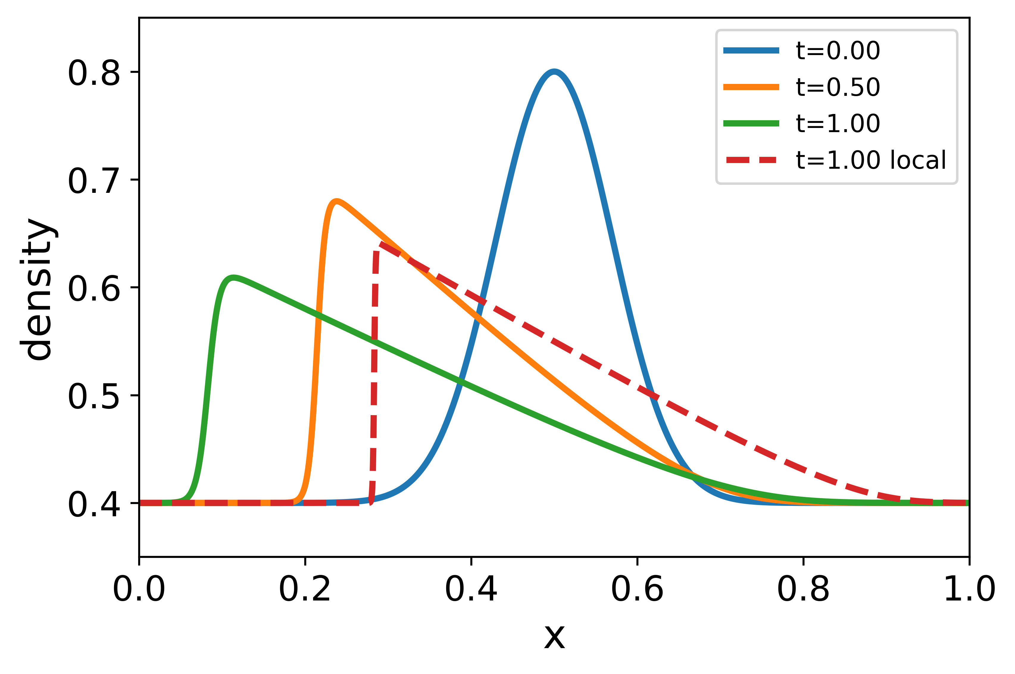
Refer to caption
Refer to caption
Refer to caption
Refer to caption
Refer to caption
Refer to caption
Figure 2: Experiment 1: Snapshots of computed solutions for the bell-shaped initial data (top) and the Riemann initial data (bottom) corresponding to the left endpoint quadrature weights (left), the normalized left endpoint quadrature weights (middle), and the exact quadrature weights (right).

For the bell-shaped initial data, we observe from the top row of Figure 2 that the numerical solutions of the nonlocal model preserve the smoothness of the initial data while the local solution develops a shock. At time t=1𝑡1t=1, the numerical solutions of the nonlocal model computed with the normalized left endpoint quadrature weights and the exact quadrature weights are close to the local solution, especially in the region away from the shock of the local solution. This means that the numerical solution ρδ,hsuperscript𝜌𝛿\rho^{\delta,h} with both δ,h𝛿\delta,h small provides a good approximation to the local solution ρ0superscript𝜌0\rho^{0}, which validates the conclusion of Theorem 2. We also observe from the top left figure of Figure 2 that the numerical solution of the nonlocal model computed with the left endpoint quadrature weights is very different from the local solution at time t=1𝑡1t=1. Although the numerical solution of the nonlocal model still approximates a shock profile at time t=1𝑡1t=1, the shock position is incorrect. The comparison between the three sets of numerical quadrature weights emphasizes the significance of the normalization condition (26) for numerical quadrature weights.

For the Riemann initial data, the local solution ρ0superscript𝜌0\rho^{0} is a traveling wave moving at the constant speed v=1(ρL+ρR)=0.3𝑣1subscript𝜌𝐿subscript𝜌𝑅0.3v=1-(\rho_{L}+\rho_{R})=0.3. We observe from the bottom row of Figure 2 that the numerical solutions of the nonlocal model computed with the normalized left endpoint quadrature weights and the exact quadrature weights are close to the local solution at time t=1𝑡1t=1. Meanwhile, in contrast to the discontinuity of the local solution, the nonlocal solutions get smoothed because of the nonlocal effects. We also observe from the bottom left figure of Figure 2 that the numerical solution of the nonlocal model computed with the left endpoint quadrature weights is very different from the local solution at time t=1𝑡1t=1. While the former still approximates a Riemann data at time t=1𝑡1t=1, the position of the jump from ρL=0.1subscript𝜌𝐿0.1\rho_{L}=0.1 to ρR=0.6subscript𝜌𝑅0.6\rho_{R}=0.6 is incorrect. The comparison again emphasizes the significance of the normalization condition (26) for numerical quadrature weights.

Experiment 2. We next check the asymptotically compatibility of the scheme (21)-(22) by plotting ρδ,hρ0𝐋1subscriptdelimited-∥∥superscript𝜌𝛿superscript𝜌0superscript𝐋1\left\lVert\rho^{\delta,h}-\rho^{0}\right\rVert_{\mathbf{L}^{1}} with δh0proportional-to𝛿0\delta\propto h\to 0. We take δ=mh𝛿𝑚\delta=mh where m=1,2,5𝑚125m=1,2,5 and h=0.01×2l0.01superscript2𝑙h=0.01\times 2^{-l} for l=0,1,2,3𝑙0123l=0,1,2,3, and compute numerical solutions ρδ,hsuperscript𝜌𝛿\rho^{\delta,h} using the Lax-Friedrichs numerical flux function (24a) and different numerical quadrature weights. The local solution ρ0superscript𝜌0\rho^{0} is numerically solved on a fine grid with h=0.01×250.01superscript25h=0.01\times 2^{-5} using a Lax-Friedrichs scheme for (1) with the numerical flux function (62). For each initial data and each set of numerical quadrature weights, we compute the 𝐋1superscript𝐋1\mathbf{L}^{1} error ρδ,hρ0𝐋1subscriptdelimited-∥∥superscript𝜌𝛿superscript𝜌0superscript𝐋1\left\lVert\rho^{\delta,h}-\rho^{0}\right\rVert_{\mathbf{L}^{1}} with an interpolation of ρδ,hsuperscript𝜌𝛿\rho^{\delta,h} onto the fine grid on which ρ0superscript𝜌0\rho^{0} is computed, and plot ρδ,hρ0𝐋1subscriptdelimited-∥∥superscript𝜌𝛿superscript𝜌0superscript𝐋1\left\lVert\rho^{\delta,h}-\rho^{0}\right\rVert_{\mathbf{L}^{1}} against h1superscript1h^{-1} in the log-log scale for δ=h𝛿\delta=h, δ=2h𝛿2\delta=2h, and δ=5h𝛿5\delta=5h in different colors. We also plot a dashed line with the slope 11-1 to represent the linear convergence rate. See the results in Figure 3.
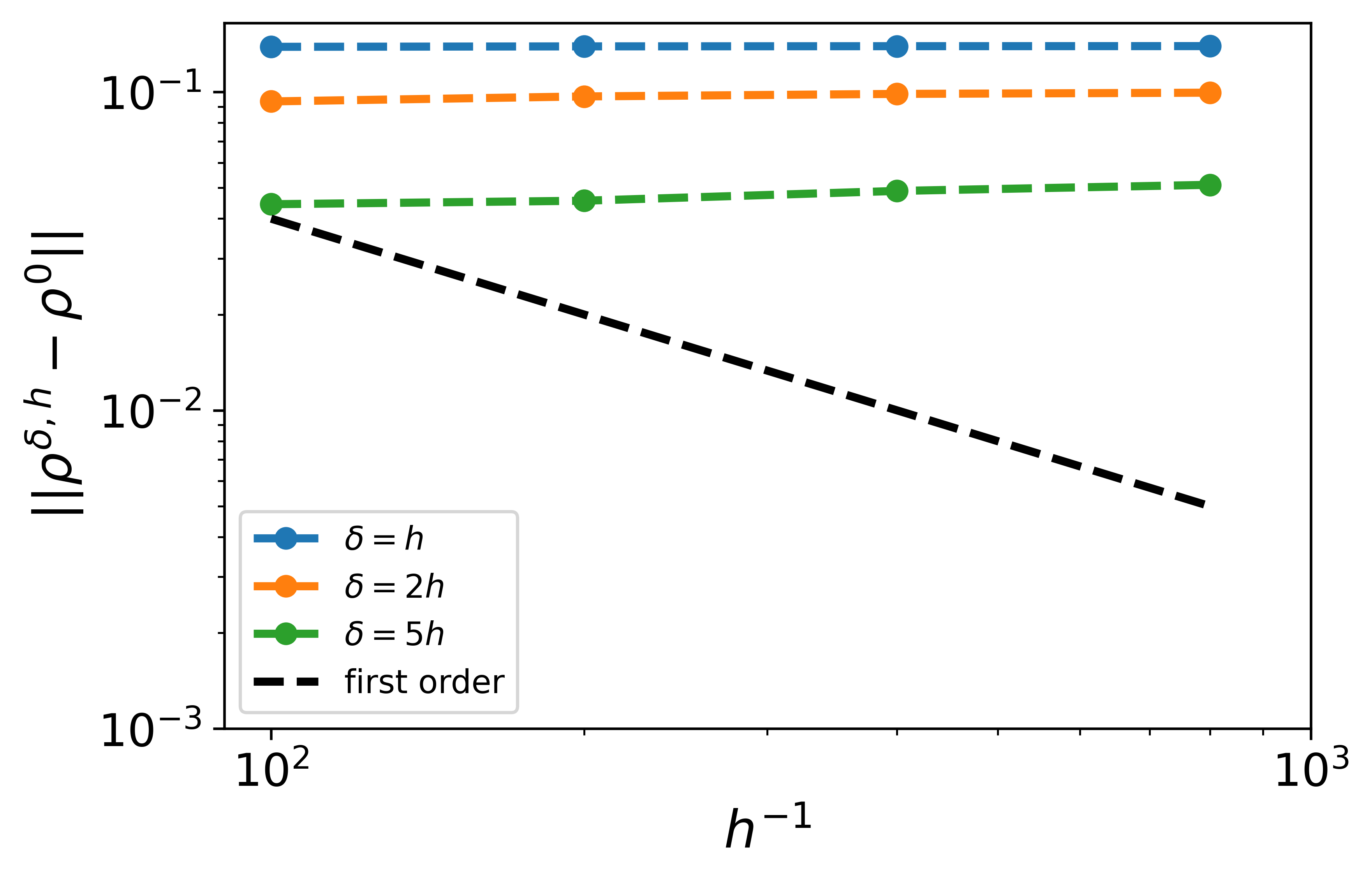
Refer to caption
Refer to caption
Refer to caption
Refer to caption
Refer to caption
Refer to caption
Figure 3: Experiment 2: Convergence from ρδ,hsuperscript𝜌𝛿\rho^{\delta,h} to ρ0superscript𝜌0\rho^{0} for the bell-shaped initial data (top) and the Riemann initial data (bottom) corresponding to the left endpoint quadrature weights (left), the normalized left endpoint quadrature weights (middle), and the exact quadrature weights (right).

We observe from Figure 3 that: for the normalized left endpoint quadrature weights and the exact quadrature weights, the error ρδ,hρ0𝐋1subscriptdelimited-∥∥superscript𝜌𝛿superscript𝜌0superscript𝐋1\left\lVert\rho^{\delta,h}-\rho^{0}\right\rVert_{\mathbf{L}^{1}} has a linear decay rate with respect to hh for both initial data and δ=mh𝛿𝑚\delta=mh for m=1,2,5𝑚125m=1,2,5. This means that ρδ,hsuperscript𝜌𝛿\rho^{\delta,h} converges to ρ0superscript𝜌0\rho^{0} along the limiting paths δ=mh0𝛿𝑚0\delta=mh\to 0 for m=1,2,5𝑚125m=1,2,5, which validates the conclusion of Theorem 2. Moreover, the numerical results show that the convergence is of first order with the particular choices of the initial data and the limiting paths. In contrast, for the left endpoint numerical quadrature weights, the error ρδ,hρ0𝐋1subscriptdelimited-∥∥superscript𝜌𝛿superscript𝜌0superscript𝐋1\left\lVert\rho^{\delta,h}-\rho^{0}\right\rVert_{\mathbf{L}^{1}} stagnates on the scale of 101superscript10110^{-1} for both initial data and δ=mh𝛿𝑚\delta=mh for m=1,2,5𝑚125m=1,2,5. This is due to the convergence of ρδ,hsuperscript𝜌𝛿\rho^{\delta,h} to an incorrect solution when δ=mh0𝛿𝑚0\delta=mh\to 0, further highlighting the importance of asymptotically compatibility via the normalization condition (26).

Experiment 3. We now check the uniform convergence of the scheme (21)-(22) with respect to δ𝛿\delta by plotting ρδ,hρδ𝐋1subscriptdelimited-∥∥superscript𝜌𝛿superscript𝜌𝛿superscript𝐋1\left\lVert\rho^{\delta,h}-\rho^{\delta}\right\rVert_{\mathbf{L}^{1}} with h00h\to 0 for different choices of δ𝛿\delta. We take δ=0.01×2l𝛿0.01superscript2𝑙\delta=0.01\times 2^{-l} for l=0,1,2𝑙012l=0,1,2 and h=0.01×2l0.01superscript2𝑙h=0.01\times 2^{-l} for l=0,1,2,3𝑙0123l=0,1,2,3, and compute numerical solutions ρδ,hsuperscript𝜌𝛿\rho^{\delta,h} using the Lax-Friedrichs numerical flux function (24a) and different numerical quadrature weights. The reference solution ρδsuperscript𝜌𝛿\rho^{\delta} is numerically solved on a fine grid with h=0.01×250.01superscript25h=0.01\times 2^{-5} using the same scheme. For each initial data and each set of numerical quadrature weights, we compute the 𝐋1superscript𝐋1\mathbf{L}^{1} error ρδ,hρδ𝐋1subscriptdelimited-∥∥superscript𝜌𝛿superscript𝜌𝛿superscript𝐋1\left\lVert\rho^{\delta,h}-\rho^{\delta}\right\rVert_{\mathbf{L}^{1}} with an interpolation of ρδ,hsuperscript𝜌𝛿\rho^{\delta,h} onto the fine grid, and plot ρδ,hρδ𝐋1subscriptdelimited-∥∥superscript𝜌𝛿superscript𝜌𝛿superscript𝐋1\left\lVert\rho^{\delta,h}-\rho^{\delta}\right\rVert_{\mathbf{L}^{1}} with respect to h1superscript1h^{-1} in the log-log scale for δ=0.01𝛿0.01\delta=0.01, δ=0.005𝛿0.005\delta=0.005, and δ=0.0025𝛿0.0025\delta=0.0025 in different colors. A dashed line with the slope 11-1 is again provided. See the results in Figure 4.
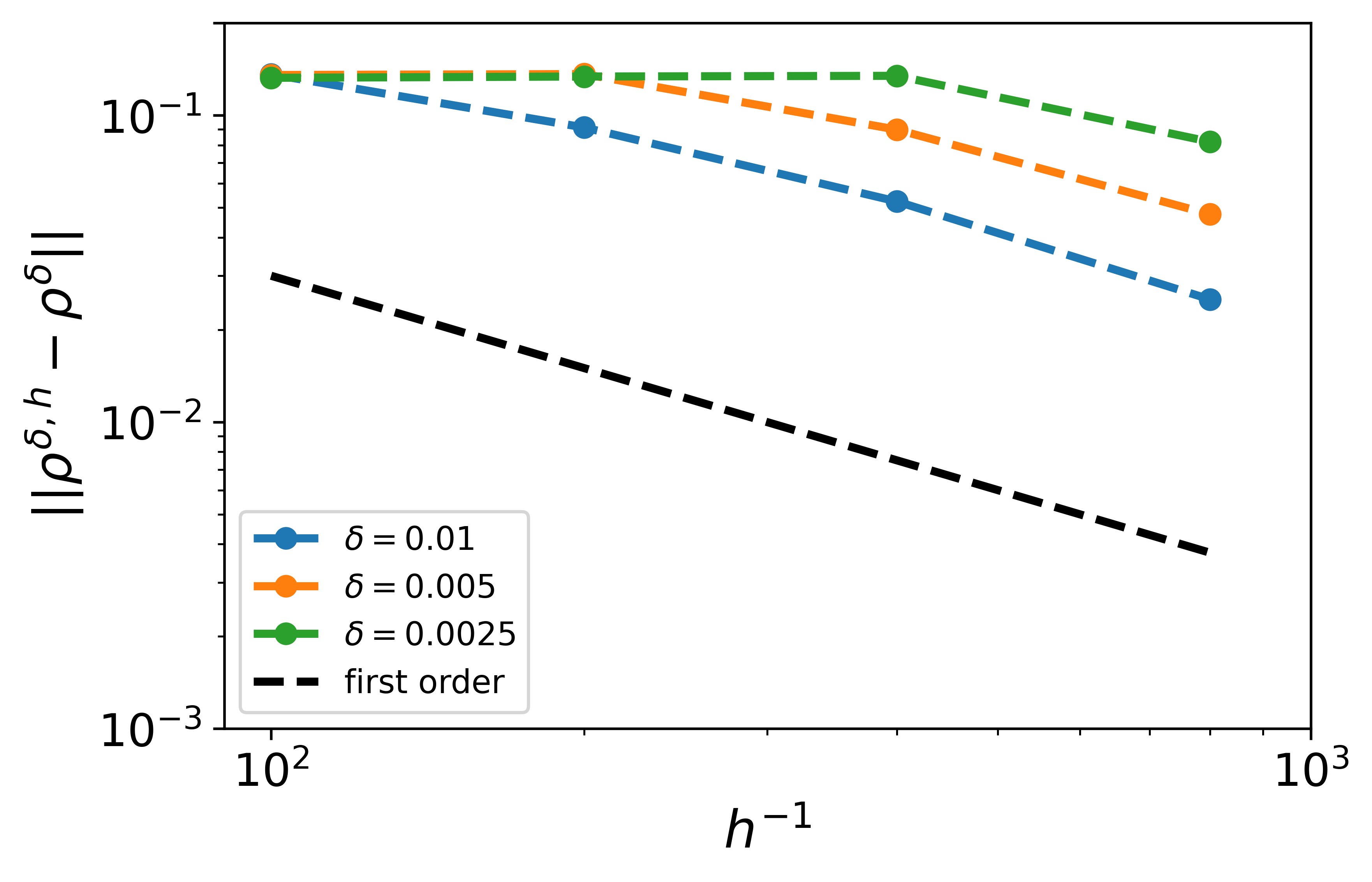
Refer to caption
Refer to caption
Refer to caption
Refer to caption
Refer to caption
Refer to caption
Figure 4: Experiment 3: Convergence from ρδ,hsuperscript𝜌𝛿\rho^{\delta,h} to ρδsuperscript𝜌𝛿\rho^{\delta} for the bell-shaped initial data (top) and the Riemann initial data (bottom) corresponding to the left endpoint quadrature weights (left), the normalized left endpoint quadrature weights (middle), and the exact quadrature weights (right).

From Figure 4, we see that for the normalized left endpoint quadrature weights and the exact quadrature weights, the error ρδ,hρδ𝐋1subscriptdelimited-∥∥superscript𝜌𝛿superscript𝜌𝛿superscript𝐋1\left\lVert\rho^{\delta,h}-\rho^{\delta}\right\rVert_{\mathbf{L}^{1}} has a linear decay rate with respect to hh for both initial data and all choices of δ𝛿\delta. Moreover, the plots of ρδ,hρδ𝐋1subscriptdelimited-∥∥superscript𝜌𝛿superscript𝜌𝛿superscript𝐋1\left\lVert\rho^{\delta,h}-\rho^{\delta}\right\rVert_{\mathbf{L}^{1}} with respect to h1superscript1h^{-1} have very little change for δ=0.01𝛿0.01\delta=0.01, δ=0.005𝛿0.005\delta=0.005, and δ=0.0025𝛿0.0025\delta=0.0025. This means that ρδ,hsuperscript𝜌𝛿\rho^{\delta,h} converges to ρδsuperscript𝜌𝛿\rho^{\delta} as h00h\to 0 uniformly in δ𝛿\delta, which validates the conclusion of Theorem 3. In addition, the numerical results show that the convergence is of first order with the particular choices of the initial data and the parameter δ𝛿\delta. In contrast, for the left endpoint numerical quadrature weights, the error ρδ,hρδ𝐋1subscriptdelimited-∥∥superscript𝜌𝛿superscript𝜌𝛿superscript𝐋1\left\lVert\rho^{\delta,h}-\rho^{\delta}\right\rVert_{\mathbf{L}^{1}} stagnates on the scale of 101superscript10110^{-1} when hδ𝛿h\geq\delta for both initial data and all choices of δ𝛿\delta. This may because ρδsuperscript𝜌𝛿\rho^{\delta} approximates ρ0superscript𝜌0\rho^{0} well when δ𝛿\delta is small while ρδ,h=ρ0,hsuperscript𝜌𝛿superscript𝜌0\rho^{\delta,h}=\rho^{0,h} when hδ𝛿h\geq\delta and ρ0,hsuperscript𝜌0\rho^{0,h} is not a consistent numerical approximation to ρ0superscript𝜌0\rho^{0}. We also observe that, in each case, the error decays when h<δ𝛿h<\delta. However, the error increases when δ𝛿\delta decreases from 0.010.010.01 to 0.00250.00250.0025 for any fixed mesh size hh. One can infer that the convergence from ρδ,hsuperscript𝜌𝛿\rho^{\delta,h} to ρδsuperscript𝜌𝛿\rho^{\delta} as h00h\to 0 will become slower and slower as δ0𝛿0\delta\to 0, and the uniform convergence cannot hold, which is again showing the importance of the normalization condition (26) for the uniform convergence of the scheme (21)-(22).

Experiment 4. We finally test the scheme (21)-(22) with different choices of the nonlocal kernel. Besides the linear decreasing kernel considered before, we also use the exponential kernel wδ(s)=esδδ(1e1)subscript𝑤𝛿𝑠superscript𝑒𝑠𝛿𝛿1superscript𝑒1w_{\delta}(s)=\frac{e^{-\frac{s}{\delta}}}{\delta(1-e^{-1})} and the constant kernel wδ(s)=1δsubscript𝑤𝛿𝑠1𝛿w_{\delta}(s)=\frac{1}{\delta}, and adopt the exact quadrature weights (19). We take δ=mh𝛿𝑚\delta=mh where m=1,2,5𝑚125m=1,2,5 and h=0.01×2l0.01superscript2𝑙h=0.01\times 2^{-l} for l=0,1,2,3𝑙0123l=0,1,2,3, and compute numerical solutions ρδ,hsuperscript𝜌𝛿\rho^{\delta,h} using the Lax-Friedrichs numerical flux function (24a) and different numerical quadrature weights. The local solution ρ0superscript𝜌0\rho^{0} is numerically solved on a fine grid with h=0.01×250.01superscript25h=0.01\times 2^{-5} using a Lax-Friedrichs scheme for (1) with the numerical flux function (62). For each initial data and each nonlocal kernel, we compute the 𝐋1superscript𝐋1\mathbf{L}^{1} error ρδ,hρ0𝐋1subscriptdelimited-∥∥superscript𝜌𝛿superscript𝜌0superscript𝐋1\left\lVert\rho^{\delta,h}-\rho^{0}\right\rVert_{\mathbf{L}^{1}}. A dashed line with the slope 11-1 is again provided. See the results in Figure 5.
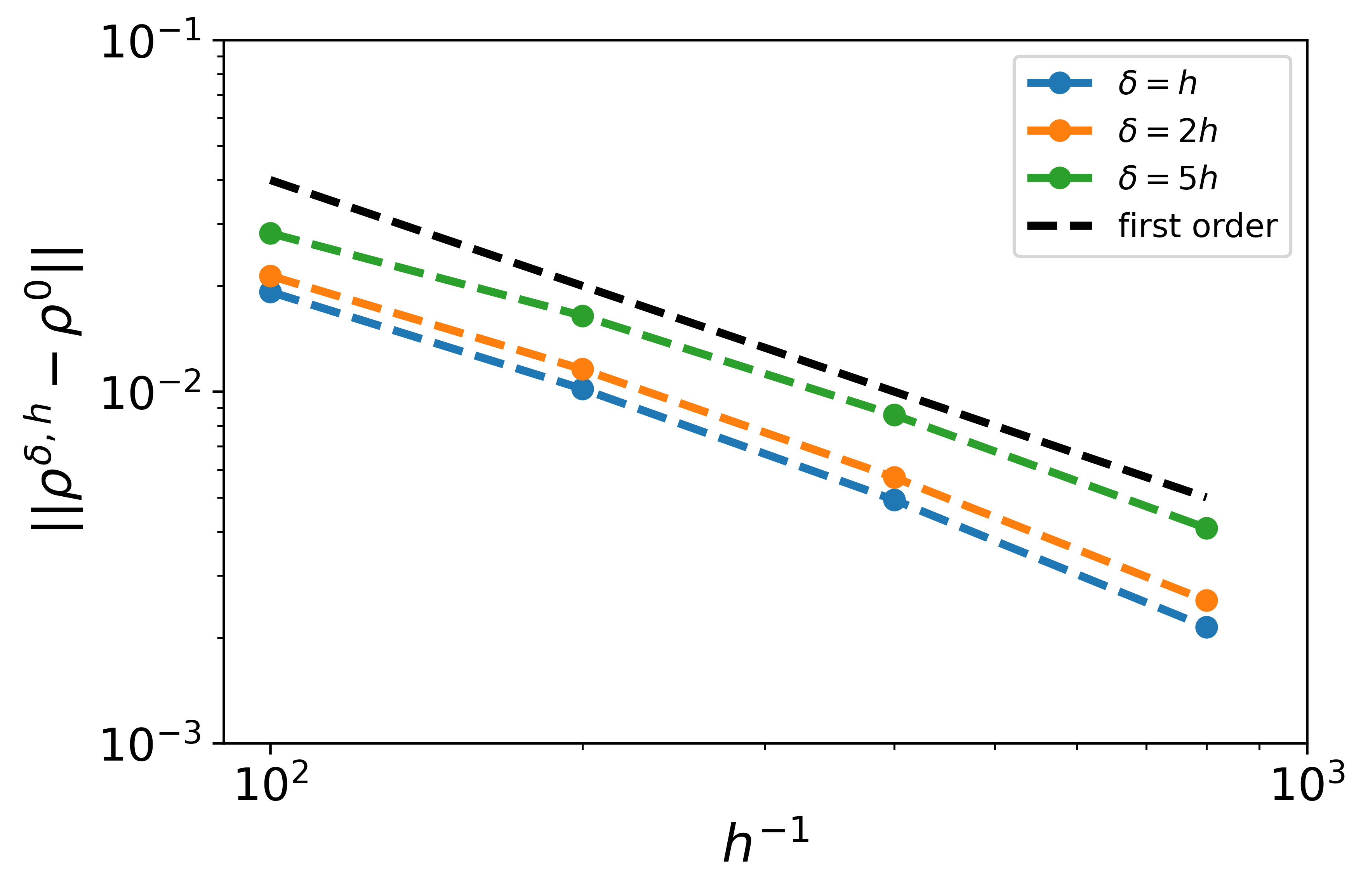
Refer to caption
Refer to caption
Refer to caption
Refer to caption
Refer to caption
Refer to caption
Figure 5: Experiment 4: Convergence from ρδ,hsuperscript𝜌𝛿\rho^{\delta,h} to ρ0superscript𝜌0\rho^{0} for the bell-shaped initial data (top) and the Riemann initial data (bottom) corresponding to the linear decreasing kernel (left), the exponential kernel (middle), and the constant kernel (right).

We observe from Figure 5 that: for all the three nonlocal kernels, the error ρδ,hρ0𝐋1subscriptdelimited-∥∥superscript𝜌𝛿superscript𝜌0superscript𝐋1\left\lVert\rho^{\delta,h}-\rho^{0}\right\rVert_{\mathbf{L}^{1}} has a linear decay rate with respect to hh for both initial data and in all cases δ=mh𝛿𝑚\delta=mh for m=1,2,5𝑚125m=1,2,5. Moreover, the plots for the three nonlocal kernels have little difference. For the linear decreasing kernel and the exponential kernel, the convergence result validates the conclusion of Theorem 2. For the constant kernel, it does not satisfy the condition that w=wδ(s)𝑤subscript𝑤𝛿𝑠w=w_{\delta}(s) is strictly decreasing, and (25) does not hold because wk1wk=0subscript𝑤𝑘1subscript𝑤𝑘0w_{k-1}-w_{k}=0 for all k=1,,m1𝑘1𝑚1k=1,\cdots,m-1. In this case, the analysis used in the proof of Theorem 1 cannot give the necessary estimates on numerical solutions but the numerical results show that the conclusion of Theorem 2 may still be true.

4 Conclusions and future work

In this work, finite volume numerical schemes (21)-(22) are studied for solving the nonlocal LWR model (2) with a parameter δ𝛿\delta that measures the range of information exchange. An important observation is that, based on both numerical analysis and computational experiments, certain numerical quadrature weights that provide consistent approximations in the case of a given δ>0𝛿0\delta>0 may lead to consistency between the scheme (21)-(22) and the local limit (1) of the nonlocal model (2) as δ0𝛿0\delta\to 0 and h00h\to 0. For properly selected numerical quadrature weights, we are able to prove, under reasonable assumptions that the numerical solutions of the nonlocal model converge to the continuum solution of the nonlocal model with a fixed δ>0𝛿0\delta>0 as h00h\to 0, while they converge to the entropy solution of the local continuum model (1) as δ0𝛿0\delta\to 0 and h00h\to 0 simultaneously. That is, such schemes are asymptotically compatible with its local limit. We are able to demonstrate that these asymptotically compatible schemes can offer robust numerical simulations under the changes in δ𝛿\delta due to the uniform convergence when the values of δ𝛿\delta are within a proper range.

Our established results are based on the a priori estimates on the numerical solutions as given in Theorem 1, subject to assumptions alluded to above. As shown in the computational experiments, the normalization condition for numerical quadrature weights is essential to the asymptotically compatibility of the scheme (21)-(22). The experiments also suggest that the results of this work may be extended to the cases with more general nonlocal kernels and numerical flux functions. It might also be possible to establish the results with more general velocity functions v=v(ρ)𝑣𝑣𝜌v=v(\rho) other than the linear one v(ρ)=1ρ𝑣𝜌1𝜌v(\rho)=1-\rho used here and also more general initial data that may have negative jumps. Furthermore, with the a priori bounds on the numerical solutions and known estimates on the exact solutions, it is possible to derive a priori error estimates subject to suitable conditions on the regularities of continuum solutions. These questions along with further generalizations and applications of nonlocal traffic flow models will be subjects of future research.

References

  • [1] A. Aggarwal, R. M. Colombo, and P. Goatin, Nonlocal systems of conservation laws in several space dimensions, SIAM Journal on Numerical Analysis, 53 (2015), pp. 963–983.
  • [2] P. Amorim, R. M. Colombo, and A. Teixeira, On the numerical integration of scalar nonlocal conservation laws, ESAIM: Mathematical Modelling and Numerical Analysis, 49 (2015), pp. 19–37.
  • [3] F. Berthelin, , P. Goatin, and and, Regularity results for the solutions of a non-local model of traffic flow, Discrete & Continuous Dynamical Systems - A, 39 (2019), pp. 3197–3213.
  • [4] F. Betancourt, R. Bürger, K. H. Karlsen, and E. M. Tory, On nonlocal conservation laws modelling sedimentation, Nonlinearity, 24 (2011), p. 855.
  • [5] S. Blandin and P. Goatin, Well-posedness of a conservation law with non-local flux arising in traffic flow modeling, Numerische Mathematik, 132 (2016), pp. 217–241.
  • [6] Y. Brenier and S. Osher, The discrete one-sided lipschitz condition for convex scalar conservation laws, SIAM Journal on Numerical Analysis, 25 (1988), pp. 8–23.
  • [7] A. Bressan and W. Shen, Entropy admissibility of the limit solution for a nonlocal model of traffic flow, arXiv preprint arXiv:2011.05430, (2020).
  • [8]  , On traffic flow with nonlocal flux: a relaxation representation, Archive for Rational Mechanics and Analysis, 237 (2020), pp. 1213–1236.
  • [9] R. Bürger, P. Goatin, D. Inzunza, and L. M. Villada, A non-local pedestrian flow model accounting for anisotropic interactions and walking domain boundaries, Mathematical biosciences and engineering, 17 (2020), pp. 5883–5906.
  • [10] C. Chalons, P. Goatin, and L. M. Villada, High-order numerical schemes for one-dimensional nonlocal conservation laws, SIAM Journal on Scientific Computing, 40 (2018), pp. A288–A305.
  • [11] F. A. Chiarello, P. Goatin, and E. Rossi, Stability estimates for non-local scalar conservation laws, Nonlinear Analysis: Real World Applications, 45 (2019), pp. 668–687.
  • [12] G. M. Coclite, J.-M. Coron, N. De Nitti, A. Keimer, and L. Pflug, A general result on the approximation of local conservation laws by nonlocal conservation laws: The singular limit problem for exponential kernels, Annales de l’Institut Henri Poincaré C, (2022).
  • [13] M. Colombo, G. Crippa, M. Graff, and L. V. Spinolo, On the role of numerical viscosity in the study of the local limit of nonlocal conservation laws, ESAIM: Mathematical Modelling and Numerical Analysis, 55 (2021), pp. 2705–2723.
  • [14] M. Colombo, G. Crippa, E. Marconi, and L. V. Spinolo, Local limit of nonlocal traffic models: convergence results and total variation blow-up, Annales de l’Institut Henri Poincaré C, Analyse non linéaire, 38 (2021), pp. 1653–1666.
  • [15]  , Nonlocal traffic models with general kernels: singular limit, entropy admissibility, and convergence rate, arXiv preprint arXiv:2206.03949, (2022).
  • [16] M. Colombo, G. Crippa, and L. V. Spinolo, On the singular local limit for conservation laws with nonlocal fluxes, Archive for Rational Mechanics and Analysis, 233 (2019), pp. 1131–1167.
  • [17] R. M. Colombo, M. Garavello, and M. Lécureux-Mercier, A class of nonlocal models for pedestrian traffic, Mathematical Models and Methods in Applied Sciences, 22 (2012), p. 1150023.
  • [18] R. M. Colombo and E. Rossi, Nonlocal conservation laws in bounded domains, SIAM Journal on Mathematical Analysis, 50 (2018), pp. 4041–4065.
  • [19] L. C. Evans and R. F. Garzepy, Measure theory and fine properties of functions, Routledge, 2018.
  • [20] F. Filbet and S. Jin, A class of asymptotic-preserving schemes for kinetic equations and related problems with stiff sources, Journal of Computational Physics, 229 (2010), pp. 7625–7648.
  • [21] J. Friedrich, S. Göttlich, and M. Herty, Lyapunov stabilization for nonlocal traffic flow models, arXiv preprint arXiv:2209.05256, (2022).
  • [22] J. Friedrich, S. Göttlich, A. Keimer, and L. Pflug, Conservation laws with nonlocal velocity–the singular limit problem, arXiv preprint arXiv:2210.12141, (2022).
  • [23] J. Friedrich and O. Kolb, Maximum principle satisfying cweno schemes for nonlocal conservation laws, SIAM Journal on Scientific Computing, 41 (2019), pp. A973–A988.
  • [24] J. Friedrich, O. Kolb, and S. Göttlich, A godunov type scheme for a class of lwr traffic flow models with non-local flux, arXiv preprint arXiv:1802.07484, (2018).
  • [25] P. Goatin and E. Rossi, Well-posedness of IBVP for 1D scalar non-local conservation laws, ZAMM-Journal of Applied Mathematics and Mechanics/Zeitschrift für Angewandte Mathematik und Mechanik, 99 (2019), p. e201800318.
  • [26] P. Goatin and S. Scialanga, Well-posedness and finite volume approximations of the LWR traffic flow model with non-local velocity, Networks and Hetereogeneous Media, 11 (2016), pp. 107–121.
  • [27] S. Göttlich, S. Hoher, P. Schindler, V. Schleper, and A. Verl, Modeling, simulation and validation of material flow on conveyor belts, Applied mathematical modelling, 38 (2014), pp. 3295–3313.
  • [28] K. Huang and Q. Du, Stability of a nonlocal traffic flow model for connected vehicles, SIAM Journal on Applied Mathematics, 82 (2022), pp. 221–243.
  • [29] S. Jin, Efficient asymptotic-preserving (ap) schemes for some multiscale kinetic equations, SIAM Journal on Scientific Computing, 21 (1999), pp. 441–454.
  • [30]  , Asymptotic preserving (ap) schemes for multiscale kinetic and hyperbolic equations: a review, Lecture notes for summer school on methods and models of kinetic theory (M&MKT), Porto Ercole (Grosseto, Italy), (2010), pp. 177–216.
  • [31] I. Karafyllis, D. Theodosis, and M. Papageorgiou, Analysis and control of a non-local PDE traffic flow model, International Journal of Control, 0 (2020), pp. 1–34.
  • [32] A. Keimer and L. Pflug, On approximation of local conservation laws by nonlocal conservation laws, Journal of Mathematical Analysis and Applications, 475 (2019), pp. 1927–1955.
  • [33]  , On the singular limit problem for a discontinuous nonlocal conservation law, arXiv preprint arXiv:2212.12598, (2022).
  • [34] P. G. LeFloch, Hyperbolic Systems of Conservation Laws: The theory of classical and nonclassical shock waves, Springer Science & Business Media, 2002.
  • [35] R. J. LeVeque et al., Finite volume methods for hyperbolic problems, vol. 31, Cambridge university press, 2002.
  • [36] M. J. Lighthill and G. B. Whitham, On kinematic waves II. A theory of traffic flow on long crowded roads, Proc. R. Soc. Lond. A, 229 (1955), pp. 317–345.
  • [37] P. I. Richards, Shock waves on the highway, Operations research, 4 (1956), pp. 42–51.
  • [38] J. Ridder and W. Shen, Traveling waves for nonlocal models of traffic flow, Discrete & Continuous Dynamical Systems-A, 39 (2019), p. 4001.
  • [39] E. Rossi, J. Weißen, P. Goatin, and S. Göttlich, Well-posedness of a non-local model for material flow on conveyor belts, ESAIM: Mathematical Modelling and Numerical Analysis, 54 (2020), pp. 679–704.
  • [40] W. Shen, Traveling waves for conservation laws with nonlocal flux for traffic flow on rough roads, Networks and Heterogeneous Media, 14 (2019), pp. 709–732.
  • [41] E. Tadmor, The large-time behavior of the scalar, genuinely nonlinear lax-friedrichs scheme, Mathematics of computation, 43 (1984), pp. 353–368.
  • [42] X. Tian and Q. Du, Asymptotically compatible schemes and applications to robust discretization of nonlocal models, SIAM Journal on Numerical Analysis, 52 (2014), pp. 1641–1665.
  • [43]  , Asymptotically compatible schemes for robust discretization of parametrized problems with applications to nonlocal models, SIAM Review, 62 (2020), pp. 199–227.