Sparse Array Design for Dual-Function Radar-Communications System

Huiping Huang, Student Member, IEEE, Linlong Wu, Member, IEEE, Bhavani Shankar, Senior Member, IEEE, and Abdelhak M. Zoubir, Fellow, IEEE The work of H. Huang was supported by the Graduate School CE within the Centre for Computational Engineering at Technische Universität Darmstadt. The work of L. Wu and B. Shankar was supported by FNR through the CORE SPRINGER project under Grant C18/IS/12734677. (Corresponding author: Linlong Wu)H. Huang was with Technische Universität Darmstadt, Darmstadt, Germany; and now is with Chalmers University of Technology, Gothenburg, Sweden (e-mail: huiping@chalmers.se).L. Wu and B. Shankar are with University of Luxembourg, Luxembourg City, Luxembourg (e-mail: {linlong.wu; Bhavani.Shankar}@uni.lu).A. M. Zoubir is with Technische Universität Darmstadt, Darmstadt, Germany (e-mail: zoubir@spg.tu-darmstadt.de).
Abstract

The problem of sparse array design for dual-function radar-communications is investigated. Our goal is to design a sparse array which can simultaneously shape desired beam responses and serve multiple downlink users with the required signal-to-interference-plus-noise ratio levels. Besides, we also take into account the limitation of the radiated power by each antenna. The problem is formulated as a quadratically constrained quadratic program with a joint-sparsity-promoting regularization, which is NP-hard. The resulting problem is solved by the consensus alternating direction method of multipliers, which enjoys parallel implementation. Numerical simulations exhibit the effectiveness and superiority of the proposed method which leads to a more power-efficient solution.

Index Terms:
Alternating direction method of multipliers, dual-funtion radar-communications, sparse array design

I Introduction

Dual-function radar-communications (DFRC) systems have been recently widely investigated [1, 2, 3, 4]. They find applications in a wide range of areas, including vehicular networks, indoor positioning and covert communications [5, 6]. To achieve accurate sensing and high throughput, the DFRC systems probably require a large number of antennas [7, 8, 9, 10]. In practice, a base station usually equips with less radio-frequency (RF) chains than antennas given the hardware cost consideration. For such a configuration, it raises a question on how to adaptively switch the available RF chains to the corresponding subset of antennas [11, 12, 13], which can be interpreted as sparse array design.

In this work, we consider the sparse array design for the DFRC system. Similar problems have been studied in [14, 15, 16, 17, 18, 19]. The authors in [14] derived a Cramér-Rao bound for the cooperative radar‐communications system, where they focused on target parameter estimation. The work [15] developed an antenna selection strategy by using a learning approach. This method requires a training process, which might be unavailable in some practical applications. The authors in [16] introduced a realistic waveform constraint in the DFRC system, in order to improve the power efficiency. A surrogate subproblem instead of the original problem was solved, which might lead to a highly suboptimal solution. In [17] and [18], several types of DFRC systems were proposed which implement simultaneous beamformers associated with single and different sparse arrays with shared aperture. However, these two works consider a single-user case, and the corresponding methods cannot be applicable to the case of multi-users. A weighted 1,qsubscript1𝑞\ell_{1,q}-norm optimization based approach was developed in [19]. Note that all the problems considered in [17, 18, 19] are convex and were solved by the existing toolbox such as CVX.

Unlike in previous works, we propose a novel system model for DFRC systems, and formulate the corresponding sparse array design problem as a quadratically constrained quadratic program (QCQP) regularized by a joint-sparsity-promoting term. Besides the control on illumination beampattern and communication signal-to-interference-plus-noise ratio (SINR), we also take into account the limitation of the radiated power by each antenna. We propose an algorithm based on the consensus alternating direction method of multipliers (ADMM) to solve the resulting problem. Note that at each ADMM iteration, the primary variable has a closed-form solution, and the auxiliary variables can be solved efficiently in a parallel manner. Simulation results show its superior performance compared to other examined methods.

It is worth mentioning that the sparse array beamforming can be incorporated into the framework of hybrid beamforming, via decomposing the sparse array beamformer into the baseband beamformer with a particular selection preference and the RF beamformer. Therefore, it can further improve the power efficiency within the hybrid beamforming.

The remainder of the paper is organized as follows. The system model is established in Section II. The proposed algorithm is presented in Section III. Simulation results are shown in Section IV, while Section V concludes the paper.

Notations: Throughout this paper, bold-faced lower-case (upper-case) letters denote vectors (matrices). Superscripts TsuperscriptT\cdot^{\mathrm{T}}, HsuperscriptH\cdot^{\mathrm{H}}, superscript\cdot^{*}, 1superscript1\cdot^{-1} denote transpose, Hermitian transpose, conjugate, and inverse, respectively. E{}E\mathrm{E}\{\cdot\} denotes the expectation operator. |||\cdot| and \angle\cdot are the modulus and phase, respectively, both in an element-wise manner. \mathbb{C} and \mathbb{R} are the sets of complex and real numbers, respectively, and ȷ=1italic-ȷ1\jmath=\sqrt{-1}. 0\|\cdot\|_{0}, 1\|\cdot\|_{1}, and 2\|\cdot\|_{2} are 0subscript0\ell_{0}-quasi-norm, 1subscript1\ell_{1}-norm, and 2subscript2\ell_{2}-norm, respectively. tensor-product\otimes denotes the Kronecker product. \oslash is the element-wise division operator. 𝐈Nsubscript𝐈𝑁{\bf I}_{N} and 𝐎M×Nsubscript𝐎𝑀𝑁{\bf O}_{M\times N} are the N×N𝑁𝑁N\times N identity matrix and M×N𝑀𝑁M\times N zero matrix, respectively. 𝟏1{\bf 1} and 𝟎0{\bf 0} are the all-ones and all-zeros vector of appropriate size, respectively.

II System Model and Problem Formulation

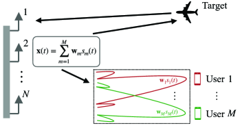
We consider a DFRC system, as indicated in Fig. 1. The transmitter, consisting of N𝑁N antennas, emits M𝑀M signals, each to a single user. The weight vector 𝐰mNsubscript𝐰𝑚superscript𝑁{\bf w}_{m}\in\mathbb{C}^{N} is designed to transfer the data symbol, sm(t)subscript𝑠𝑚𝑡s_{m}(t), to user m𝑚m, m=1,2,,Mfor-all𝑚12𝑀\forall m=1,2,\cdots\!,M. All the M𝑀M transmitted signals are also received by a target. The total transmitted signal can then be formulated as

𝐱(t)=m=1M𝐰msm(t),𝐱𝑡superscriptsubscript𝑚1𝑀subscript𝐰𝑚subscript𝑠𝑚𝑡\displaystyle{\bf x}(t)=\sum_{m=1}^{M}{\bf w}_{m}s_{m}(t), (1)

where t𝑡t is the time index. We assume that the data symbols, sm(t)subscript𝑠𝑚𝑡s_{m}(t) m=1,2,,Mfor-all𝑚12𝑀\forall m=1,2,\cdots\!,M, are mutually uncorrelated, and each sm(t)subscript𝑠𝑚𝑡s_{m}(t) is zero-mean, spatially white with unit variance, i.e.,

E{|sm(t)|2}=Esuperscriptsubscript𝑠𝑚𝑡2absent\displaystyle\mathrm{E}\{|s_{m}(t)|^{2}\}= 1,m=1,2,,M,formulae-sequence1for-all𝑚12𝑀\displaystyle~{}\!1,~{}\forall m\!=\!1,2,\cdots\!,M, (2a)
E{|si(t)sj(t)|}=Esubscript𝑠𝑖𝑡superscriptsubscript𝑠𝑗𝑡absent\displaystyle\mathrm{E}\{|s_{i}(t)s_{j}^{*}(t)|\}= 0,i,j=1,2,,M, ​and ij.formulae-sequence0for-all𝑖𝑗12𝑀 ​and 𝑖𝑗\displaystyle~{}\!0,~{}\forall i,j\!=\!1,2,\cdots\!,M,\text{~{}\!and~{}}i\!\neq\!j. (2b)

Refer to caption

Figure 1: Illustration of a DFRC system.

For the radar system, we wish to focus the transmit energy on a certain angular region, say \mathcal{B}, in order to have a higher probability of detecting the target(s) lying therein. To this end, we expect that the array response within \mathcal{B} is not less than a preset threshold, while the response outside \mathcal{B} (denoted as ¯¯\bar{\mathcal{B}}) is not higher than a small threshold. Mathematically,

E{𝐱H(t)𝐚(θi)𝐚H(θi)𝐱(t)}Esuperscript𝐱H𝑡𝐚subscript𝜃𝑖superscript𝐚Hsubscript𝜃𝑖𝐱𝑡\displaystyle\mathrm{E}\!\left\{{\bf x}^{\mathrm{H}}(t){\bf a}(\theta_{i}){\bf a}^{\mathrm{H}}(\theta_{i}){\bf x}(t)\right\} ϵp,θi,formulae-sequenceabsentsubscriptitalic-ϵpfor-allsubscript𝜃𝑖\displaystyle\geq\epsilon_{{\mathrm{p}}},~{}\forall\theta_{i}\in\mathcal{B}, (3a)
E{𝐱H(t)𝐚(θj)𝐚H(θj)𝐱(t)}Esuperscript𝐱H𝑡𝐚subscript𝜃𝑗superscript𝐚Hsubscript𝜃𝑗𝐱𝑡\displaystyle\mathrm{E}\!\left\{{\bf x}^{\mathrm{H}}(t){\bf a}(\theta_{j}){\bf a}^{\mathrm{H}}(\theta_{j}){\bf x}(t)\right\} ϵs,θj¯,formulae-sequenceabsentsubscriptitalic-ϵsfor-allsubscript𝜃𝑗¯\displaystyle\leq\epsilon_{{\mathrm{s}}},~{}\forall\theta_{j}\in\bar{\mathcal{B}}, (3b)

where 𝐚(θ)𝐚𝜃{\bf a}(\theta) denotes the steering vector of θ𝜃{\theta}, ϵpsubscriptitalic-ϵp\epsilon_{{\mathrm{p}}} and ϵssubscriptitalic-ϵs\epsilon_{{\mathrm{s}}} are two preset thresholds corresponding to the mainlobe and sidelobe, respectively. Substituting (1) and (2) into (3), we have

m=1M𝐰mH𝐚(θi)𝐚H(θi)𝐰msuperscriptsubscript𝑚1𝑀superscriptsubscript𝐰𝑚H𝐚subscript𝜃𝑖superscript𝐚Hsubscript𝜃𝑖subscript𝐰𝑚\displaystyle\sum_{m=1}^{M}{\bf w}_{m}^{\mathrm{H}}{\bf a}(\theta_{i}){\bf a}^{\mathrm{H}}(\theta_{i}){\bf w}_{m} ϵp,θi,formulae-sequenceabsentsubscriptitalic-ϵpfor-allsubscript𝜃𝑖\displaystyle\geq\epsilon_{{\mathrm{p}}},~{}\forall\theta_{i}\in\mathcal{B}, (4a)
m=1M𝐰mH𝐚(θj)𝐚H(θj)𝐰msuperscriptsubscript𝑚1𝑀superscriptsubscript𝐰𝑚H𝐚subscript𝜃𝑗superscript𝐚Hsubscript𝜃𝑗subscript𝐰𝑚\displaystyle\sum_{m=1}^{M}{\bf w}_{m}^{\mathrm{H}}{\bf a}(\theta_{j}){\bf a}^{\mathrm{H}}(\theta_{j}){\bf w}_{m} ϵs,θj¯.formulae-sequenceabsentsubscriptitalic-ϵsfor-allsubscript𝜃𝑗¯\displaystyle\leq\epsilon_{{\mathrm{s}}},~{}\forall\theta_{j}\in\bar{\mathcal{B}}. (4b)

For the downlink communication systems, the received data by the m𝑚m-th user is given as

ym(t)=𝐡mH𝐰msm(t)communication signal+j=1,jmM𝐡mH𝐰jsj(t)interference signals+nm(t)noise,subscript𝑦𝑚𝑡subscriptsuperscriptsubscript𝐡𝑚Hsubscript𝐰𝑚subscript𝑠𝑚𝑡communication signalsubscriptsuperscriptsubscriptformulae-sequence𝑗1𝑗𝑚𝑀superscriptsubscript𝐡𝑚Hsubscript𝐰𝑗subscript𝑠𝑗𝑡interference signalssubscriptsubscript𝑛𝑚𝑡noise\displaystyle y_{m}(t)=\underbrace{{\bf h}_{m}^{\mathrm{H}}{\bf w}_{m}s_{m}(t)}_{\text{communication signal}}+\underbrace{\sum_{\begin{subarray}{c}j=1,j\neq m\end{subarray}}^{M}\!\!{\bf h}_{m}^{\mathrm{H}}{\bf w}_{j}s_{j}(t)}_{\text{interference signals}}+\underbrace{n_{m}(t)}_{\text{noise}}, (5)

where nm(t)subscript𝑛𝑚𝑡n_{m}(t) is the additive white Gaussian noise with mean zero and known variance σm2superscriptsubscript𝜎𝑚2\sigma_{m}^{2}, m=1,2,,Mfor-all𝑚12𝑀\forall m=1,2,\cdots\!,M. Besides, 𝐡mNsubscript𝐡𝑚superscript𝑁{\bf h}_{m}\in\mathbb{C}^{N} denotes the channel state information (CSI) vector, which models the propagation loss and phase shift of the frequency-flat quasi-static channel from the transmitter to the m𝑚m-th user. The CSI, {𝐡m}msubscriptsubscript𝐡𝑚𝑚\{{\bf h}_{m}\}_{m}, is assumed to be perfectly available at the transmitter. The maximum power radiated by each antenna n𝑛n is given by Pnsubscript𝑃𝑛P_{n}. Therefore, we have [7]

m=1M𝐰mH𝐄n𝐰mPn,n=1,2,,N,formulae-sequencesuperscriptsubscript𝑚1𝑀superscriptsubscript𝐰𝑚Hsubscript𝐄𝑛subscript𝐰𝑚subscript𝑃𝑛for-all𝑛12𝑁\displaystyle\sum_{m=1}^{M}{\bf w}_{m}^{\mathrm{H}}{\bf E}_{n}{\bf w}_{m}\leq P_{n},~{}\forall n=1,2,\cdots\!,N, (6)

where 𝐄nsubscript𝐄𝑛{\bf E}_{n} is the N×N𝑁𝑁N\times N all-zero matrix except the n𝑛n-th diagonal entry being 111. The received SINR of user m𝑚m is defined below, and a certain minimum SINR needs to be guaranteed, i.e.,

SINRm|𝐡mH𝐰m|2jm|𝐡mH𝐰j|2+σm2γm,m=1,,M,formulae-sequencesubscriptSINR𝑚superscriptsuperscriptsubscript𝐡𝑚Hsubscript𝐰𝑚2subscript𝑗𝑚superscriptsuperscriptsubscript𝐡𝑚Hsubscript𝐰𝑗2superscriptsubscript𝜎𝑚2subscript𝛾𝑚for-all𝑚1𝑀\displaystyle\text{SINR}_{m}\!\triangleq\!\frac{\left|{\bf h}_{m}^{\mathrm{H}}{\bf w}_{m}\right|^{2}}{\sum_{j\neq m}\left|{\bf h}_{m}^{\mathrm{H}}{\bf w}_{j}\right|^{2}\!+\!\sigma_{m}^{2}}\!\geq\!\gamma_{m},~{}\forall m=1,\cdots\!,M, (7)

where jmsubscript𝑗𝑚\sum_{j\neq m} is short notation for j=1,jmMsuperscriptsubscriptformulae-sequence𝑗1𝑗𝑚𝑀\sum_{j=1,j\neq m}^{M}.

Now we consider the scenario where only KN𝐾𝑁K\leq N RF chains are available, and thus only K𝐾K antennas can be simultaneously utilized in the DFRC system. Therefore, 𝐰msubscript𝐰𝑚{\bf w}_{m}, mfor-all𝑚\forall m, are sparse, and moreover, they share the same sparsity pattern. To fulfill this requirement, we need:

𝐰~0K,subscriptnorm~𝐰0𝐾\displaystyle\|{\widetilde{\bf w}}\|_{0}\leq K, (8)

where 𝐰~[w~1,w~2,,w~N]T~𝐰superscriptsubscript~𝑤1subscript~𝑤2subscript~𝑤𝑁T{\widetilde{\bf w}}\triangleq[{\widetilde{w}}_{1},{\widetilde{w}}_{2},\cdots\!,{\widetilde{w}}_{N}]^{\mathrm{T}} with its component defined as w~n[𝐰1(n),𝐰2(n),,𝐰M(n)]2subscript~𝑤𝑛subscriptnormsubscript𝐰1𝑛subscript𝐰2𝑛subscript𝐰𝑀𝑛2{\widetilde{w}}_{n}\triangleq\|[{\bf w}_{1}(n),{\bf w}_{2}(n),\cdots\!,{\bf w}_{M}(n)]\|_{2} n=1,2,,Nfor-all𝑛12𝑁\forall n=1,2,\cdots,N, and 𝐰m(n)subscript𝐰𝑚𝑛{\bf w}_{m}(n) being the n𝑛n-th entry of vector 𝐰msubscript𝐰𝑚{\bf w}_{m}, m=1,2,,Mfor-all𝑚12𝑀\forall m=1,2,\cdots\!,M.

The quality of service (QoS) problem aims at minimizing the total transmit power (TxPower), with several constraints described above. To this end, the QoS problem is given as

min{𝐰m}subscriptsubscript𝐰𝑚\displaystyle\min_{\{{\bf w}_{m}\}}~{} TxPowerm=1M𝐰m22TxPowersuperscriptsubscript𝑚1𝑀superscriptsubscriptnormsubscript𝐰𝑚22\displaystyle{\mathrm{TxPower}}\triangleq\sum_{m=1}^{M}\|{\bf w}_{m}\|_{2}^{2} (9a)
s.t.formulae-sequencest\displaystyle\mathrm{s.t.}~{}~{}~{}\! (4),(6),(7), ​and (8).467 ​and 8\displaystyle(\ref{pass_stop_band_w}),(\ref{power_antenna_constraint}),(\ref{SINR_constraint}),\text{~{}\!and~{}}(\ref{sparsity_w}). (9b)

By replacing the non-convex 0subscript0\ell_{0}-quasi-norm in (8) with the 1subscript1\ell_{1}-norm, and incorporating it into Problem (9) as a regularization term, we have

min{𝐰m}m=1M𝐰m22+η𝐰~1s.t.(4),(6), ​and (7),formulae-sequencesubscriptsubscript𝐰𝑚superscriptsubscript𝑚1𝑀superscriptsubscriptnormsubscript𝐰𝑚22𝜂subscriptnorm~𝐰1st46 ​and 7\displaystyle\min_{\{{\bf w}_{m}\}}~{}\!\!\sum_{m=1}^{M}\!\!\|{\bf w}_{m}\|_{2}^{2}+\eta\|{\widetilde{\bf w}}\|_{1}\quad\mathrm{s.t.}~{}(\ref{pass_stop_band_w}),(\ref{power_antenna_constraint}),\text{~{}\!and~{}}(\ref{SINR_constraint}), (10)

where η𝜂\eta is a parameter controlling the sparsity of the solution.

III Proposed Method

The difficulties of solving Problem (10) are twofold. First, the discorporated sparsity has a joint structure among all 𝐰msubscript𝐰𝑚{\bf w}_{m} [20], which is different from the classical sparsity and consequently, the existing solutions cannot be directly extended. Second, the constraints (4a) and (7) are nonconvex.

In what follows, we first deal with the joint-sparsity structure of the solution by reformulating the problem, and then, we develop an algorithm based on the consensus ADMM.

III-A Problem Reformulation

First of all, we define a long column vector 𝐰MN𝐰superscript𝑀𝑁{\bf w}\in\mathbb{C}^{M\!N} as 𝐰[𝐰1T,𝐰2T,,𝐰MT]T𝐰superscriptsuperscriptsubscript𝐰1Tsuperscriptsubscript𝐰2Tsuperscriptsubscript𝐰𝑀TT{\bf w}\triangleq[{\bf w}_{1}^{\mathrm{T}},{\bf w}_{2}^{\mathrm{T}},\cdots,{\bf w}_{M}^{\mathrm{T}}]^{\mathrm{T}} and define M𝑀M matrices 𝚽mN×MNsubscript𝚽𝑚superscript𝑁𝑀𝑁{\bf\Phi}_{m}\in\mathbb{R}^{N\times M\!N} as 𝚽m[𝐎N×(m1)N,𝐈N,𝐎N×(Mm)N]subscript𝚽𝑚subscript𝐎𝑁𝑚1𝑁subscript𝐈𝑁subscript𝐎𝑁𝑀𝑚𝑁{\bf\Phi}_{m}\triangleq[{\bf O}_{N\times(m-1)N},{\bf I}_{N},{\bf O}_{N\times({M}-m)N}]. Then, Problem (10) can be reformulated as

min𝐰subscript𝐰\displaystyle\min_{{\bf w}}~{} 𝐰22+η𝐰2,1superscriptsubscriptnorm𝐰22𝜂subscriptnorm𝐰21\displaystyle\|{\bf w}\|_{2}^{2}+\eta\|{\bf w}\|_{2,1} (11a)
s.t.formulae-sequencest\displaystyle\mathrm{s.t.}~{}~{}\! 𝐰H𝐀θi𝐰ϵp,θi,formulae-sequencesuperscript𝐰Hsubscript𝐀subscript𝜃𝑖𝐰subscriptitalic-ϵpfor-allsubscript𝜃𝑖\displaystyle{\bf w}^{\mathrm{H}}{\bf A}_{\theta_{i}}{\bf w}\geq\epsilon_{{\mathrm{p}}},~{}\forall\theta_{i}\in\mathcal{B}, (11b)
𝐰H𝐀θj𝐰ϵs,θj¯,formulae-sequencesuperscript𝐰Hsubscript𝐀subscript𝜃𝑗𝐰subscriptitalic-ϵsfor-allsubscript𝜃𝑗¯\displaystyle{\bf w}^{\mathrm{H}}{\bf A}_{\theta_{j}}{\bf w}\leq\epsilon_{{\mathrm{s}}},~{}\forall\theta_{j}\in\bar{\mathcal{B}}, (11c)
𝐰H𝐁n𝐰Pn,n=1,2,,N,formulae-sequencesuperscript𝐰Hsubscript𝐁𝑛𝐰subscript𝑃𝑛for-all𝑛12𝑁\displaystyle{\bf w}^{\mathrm{H}}{\bf B}_{n}{\bf w}\leq P_{n},~{}\forall n=1,2,\cdots\!,N, (11d)
𝐰H𝐂m𝐰𝐰H𝐂m¯𝐰+σm2γm,m=1,2,,M,formulae-sequencesuperscript𝐰Hsubscript𝐂𝑚𝐰superscript𝐰Hsubscript𝐂¯𝑚𝐰superscriptsubscript𝜎𝑚2subscript𝛾𝑚for-all𝑚12𝑀\displaystyle\frac{{\bf w}^{\mathrm{H}}{\bf C}_{m}{\bf w}}{{\bf w}^{\mathrm{H}}{\bf C}_{\bar{m}}{\bf w}+\sigma_{m}^{2}}\geq\gamma_{m},~{}\forall m=1,2,\cdots\!,M, (11e)

where we define 𝐀θim=1M𝚽mH𝐚(θi)𝐚H(θi)𝚽msubscript𝐀subscript𝜃𝑖superscriptsubscript𝑚1𝑀superscriptsubscript𝚽𝑚H𝐚subscript𝜃𝑖superscript𝐚Hsubscript𝜃𝑖subscript𝚽𝑚{\bf A}_{\theta_{i}}\triangleq\sum_{m=1}^{M}\!{\bf\Phi}_{m}^{\mathrm{H}}{\bf a}(\theta_{i}){\bf a}^{\mathrm{H}}(\theta_{i}){\bf\Phi}_{m}, 𝐀θjm=1M𝚽mH𝐚(θj)𝐚H(θj)𝚽msubscript𝐀subscript𝜃𝑗superscriptsubscript𝑚1𝑀superscriptsubscript𝚽𝑚H𝐚subscript𝜃𝑗superscript𝐚Hsubscript𝜃𝑗subscript𝚽𝑚{\bf A}_{\theta_{j}}\triangleq\sum_{m=1}^{M}\!{\bf\Phi}_{m}^{\mathrm{H}}{\bf a}(\theta_{j}){\bf a}^{\mathrm{H}}(\theta_{j}){\bf\Phi}_{m}, 𝐁nm=1M𝚽mH𝐄n𝚽msubscript𝐁𝑛superscriptsubscript𝑚1𝑀superscriptsubscript𝚽𝑚Hsubscript𝐄𝑛subscript𝚽𝑚{\bf B}_{n}\triangleq\sum_{m=1}^{M}\!{\bf\Phi}_{m}^{\mathrm{H}}{\bf E}_{n}{\bf\Phi}_{m}, 𝐂m𝚽mH𝐡m𝐡mH𝚽msubscript𝐂𝑚superscriptsubscript𝚽𝑚Hsubscript𝐡𝑚superscriptsubscript𝐡𝑚Hsubscript𝚽𝑚{\bf C}_{m}\triangleq{\bf\Phi}_{m}^{\mathrm{H}}{\bf h}_{m}{\bf h}_{m}^{\mathrm{H}}{\bf\Phi}_{m}, 𝐂m¯jm𝚽jH𝐡m𝐡mH𝚽jsubscript𝐂¯𝑚subscript𝑗𝑚superscriptsubscript𝚽𝑗Hsubscript𝐡𝑚superscriptsubscript𝐡𝑚Hsubscript𝚽𝑗{\bf C}_{\bar{m}}\triangleq\sum_{j\neq m}\!\!{\bf\Phi}_{j}^{\mathrm{H}}{\bf h}_{m}{\bf h}_{m}^{\mathrm{H}}{\bf\Phi}_{j}, and we have utilized m=1M𝐰m22=𝐰22superscriptsubscript𝑚1𝑀superscriptsubscriptnormsubscript𝐰𝑚22superscriptsubscriptnorm𝐰22\sum_{m=1}^{M}\|{\bf w}_{m}\|_{2}^{2}=\|{\bf w}\|_{2}^{2}, 𝐰m=𝚽m𝐰subscript𝐰𝑚subscript𝚽𝑚𝐰{\bf w}_{m}={\bf\Phi}_{m}{\bf w}, and 𝐰2,1n=1Nm=1M|𝐰m(n)|2subscriptnorm𝐰21superscriptsubscript𝑛1𝑁superscriptsubscript𝑚1𝑀superscriptsubscript𝐰𝑚𝑛2\|{\bf w}\|_{2,1}\triangleq\sum_{n=1}^{N}\sqrt{\sum_{m=1}^{M}|{\bf w}_{m}(n)|^{2}}. Further, since the denominators, 𝐰H𝐂m¯𝐰+σm2superscript𝐰Hsubscript𝐂¯𝑚𝐰superscriptsubscript𝜎𝑚2{\bf w}^{\mathrm{H}}{\bf C}_{\bar{m}}{\bf w}+\sigma_{m}^{2}, are always positive, (11e) can be written as

𝐰H𝐃m𝐰γmσm2,m=1,2,,M,formulae-sequencesuperscript𝐰Hsubscript𝐃𝑚𝐰subscript𝛾𝑚superscriptsubscript𝜎𝑚2for-all𝑚12𝑀\displaystyle{\bf w}^{\mathrm{H}}{\bf D}_{m}{\bf w}\geq\gamma_{m}\sigma_{m}^{2},~{}\forall m=1,2,\cdots\!,M, (12)

where 𝐃m𝐂mγm𝐂m¯subscript𝐃𝑚subscript𝐂𝑚subscript𝛾𝑚subscript𝐂¯𝑚{\bf D}_{m}\triangleq{\bf C}_{m}-\gamma_{m}{\bf C}_{\bar{m}}, m=1,2,,Mfor-all𝑚12𝑀\forall m=1,2,\cdots\!,M. We observe that (11b), (11c), (11d), and (12) take the form: 𝐰H𝐅𝐰fsuperscript𝐰H𝐅𝐰𝑓{\bf w}^{\mathrm{H}}{\bf F}{\bf w}\leq f. Therefore, Problem (11) can be reformulated as

min𝐰subscript𝐰\displaystyle\min_{{\bf w}}~{} 𝐰22+η𝐰2,1superscriptsubscriptnorm𝐰22𝜂subscriptnorm𝐰21\displaystyle\|{\bf w}\|_{2}^{2}+\eta\|{\bf w}\|_{2,1} (13a)
s.t.formulae-sequencest\displaystyle\mathrm{s.t.}~{}~{}\! 𝐰H𝐅l𝐰fl,l=1,2,,L,formulae-sequencesuperscript𝐰Hsubscript𝐅𝑙𝐰subscript𝑓𝑙for-all𝑙12𝐿\displaystyle{\bf w}^{\mathrm{H}}{\bf F}_{l}{\bf w}\leq f_{l},~{}\forall l=1,2,\cdots\!,L, (13b)

where the subscript lsubscript𝑙\cdot_{l} is used to indicate the l𝑙l-th constraint in Problem (11), and L𝐿L is the total number of constraints. It is worth noting that 𝐅lsubscript𝐅𝑙{\bf F}_{l} corresponding to 𝐀θisubscript𝐀subscript𝜃𝑖-{\bf A}_{\theta_{i}} is negative semidefinite, and 𝐅lsubscript𝐅𝑙{\bf F}_{l} corresponding to 𝐃msubscript𝐃𝑚-{\bf D}_{m} could be indefinite. Therefore, in general, Problem (13) is non-convex and thus NP-hard [21]. To solve this problem, we propose an algorithm based on the consensus ADMM, which is capable of handling all the constraints in parallel.

III-B Proposed Algorithm

Firstly, we formulate Problem (13) by introducing L𝐿L auxiliary variables {𝐯lMN}l=1Lsuperscriptsubscriptsubscript𝐯𝑙superscript𝑀𝑁𝑙1𝐿\{{\bf v}_{l}\in\mathbb{C}^{M\!N}\}_{l=1}^{L}, and settle the original variable 𝐰𝐰{\bf w} and the auxiliary variables {𝐯l}lsubscriptsubscript𝐯𝑙𝑙\{{\bf v}_{l}\}_{l} in a separable fashion, as

min𝐰,{𝐯l}subscript𝐰subscript𝐯𝑙\displaystyle\min_{{\bf w},\{{\bf v}_{l}\}} 𝐰22+ηLi=1L𝐯l2,1superscriptsubscriptnorm𝐰22𝜂𝐿superscriptsubscript𝑖1𝐿subscriptnormsubscript𝐯𝑙21\displaystyle~{}\|{\bf w}\|_{2}^{2}+\frac{\eta}{L}\sum_{i=1}^{L}\|{\bf v}_{l}\|_{2,1} (14a)
s.t.formulae-sequencest\displaystyle\mathrm{s.t.}~{}~{}\! 𝐯lH𝐅l𝐯lfl,𝐯l=𝐰,l=1,2,,L.formulae-sequencesuperscriptsubscript𝐯𝑙Hsubscript𝐅𝑙subscript𝐯𝑙subscript𝑓𝑙formulae-sequencesubscript𝐯𝑙𝐰for-all𝑙12𝐿\displaystyle~{}{\bf v}_{l}^{\mathrm{H}}{\bf F}_{l}{\bf v}_{l}\leq{f}_{l},~{}{\bf v}_{l}={\bf w},~{}\forall l=1,2,\cdots\!,L. (14b)

Next, we form the scaled-form augmented Lagrangian function related to the above problem, as: (𝐰,{𝐯l},{𝐮l})=𝐰22+ηLl=1L𝐯l2,1+ρ2l=1L(𝐯l𝐰+𝐮l22𝐮l22)𝐰subscript𝐯𝑙subscript𝐮𝑙superscriptsubscriptnorm𝐰22𝜂𝐿superscriptsubscript𝑙1𝐿subscriptnormsubscript𝐯𝑙21𝜌2superscriptsubscript𝑙1𝐿superscriptsubscriptnormsubscript𝐯𝑙𝐰subscript𝐮𝑙22superscriptsubscriptnormsubscript𝐮𝑙22\mathcal{L}({\bf w},\{{\bf v}_{l}\},\{{\bf u}_{l}\})=\|{\bf w}\|_{2}^{2}+\frac{\eta}{L}\!\sum_{l=1}^{L}\!\|{\bf v}_{l}\|_{2,1}+\frac{\rho}{2}\!\sum_{l=1}^{L}\!\left(\|{\bf v}_{l}\!-\!{\bf w}+{\bf u}_{l}\|_{2}^{2}-\|{\bf u}_{l}\|_{2}^{2}\right), where ρ>0𝜌0\rho>0 stands for the augmented Lagrangian parameter, and 𝐮lsubscript𝐮𝑙{\bf u}_{l} is the scaled dual variable corresponding to the equality constraint 𝐯l=𝐰subscript𝐯𝑙𝐰{\bf v}_{l}={\bf w} in Problem (14).

Finally, the consensus ADMM updating equations can be written down as

𝐰𝐰\displaystyle{\bf w} argmin𝐰𝐰22+ρ2l=1L𝐯l𝐰+𝐮l22,absentsubscript𝐰superscriptsubscriptnorm𝐰22𝜌2superscriptsubscript𝑙1𝐿superscriptsubscriptnormsubscript𝐯𝑙𝐰subscript𝐮𝑙22\displaystyle\leftarrow{\displaystyle{\arg\min_{{\bf w}}}}~{}\|{\bf w}\|_{2}^{2}+\frac{\rho}{2}\sum_{l=1}^{L}\|{\bf v}_{l}-{\bf w}+{\bf u}_{l}\|_{2}^{2}, (15a)
𝐯lsubscript𝐯𝑙\displaystyle{\bf v}_{l} {argmin𝐯lηL𝐯l2,1+ρ2𝐯l𝐰+𝐮l22s.t.𝐯lH𝐅l𝐯lfl,\displaystyle\leftarrow\left\{\!\!\!\begin{array}[]{l}{\displaystyle{\arg\min_{{\bf v}_{l}}}}~{}\frac{\eta}{L}\|{\bf v}_{l}\|_{2,1}+\frac{\rho}{2}\|{\bf v}_{l}-{\bf w}+{\bf u}_{l}\|_{2}^{2}\\ ~{}~{}~{}\mathrm{s.t.}~{}~{}~{}~{}{\bf v}_{l}^{\mathrm{H}}{\bf F}_{l}{\bf v}_{l}\leq f_{l},\end{array}\right. (15d)
𝐮lsubscript𝐮𝑙\displaystyle{\bf u}_{l} 𝐮l+𝐯l𝐰.absentsubscript𝐮𝑙subscript𝐯𝑙𝐰\displaystyle\leftarrow{\bf u}_{l}+{\bf v}_{l}-{\bf w}. (15e)

In what follows, we show how to solve 𝐰𝐰{\bf w} and 𝐯lsubscript𝐯𝑙{\bf v}_{l} from (15a) and (15d), respectively. We start by solving 𝐰𝐰{\bf w} from (15a). It is straightforward to see that, by calculating the derivative of the objective function of (15a) with respect to (w.r.t.) 𝐰𝐰{\bf w} and setting it to 𝟎0{\bf 0}, we obtain the solution to (15a) as

𝐰^=ρ2+ρLl=1L(𝐯l+𝐮l).^𝐰𝜌2𝜌𝐿superscriptsubscript𝑙1𝐿subscript𝐯𝑙subscript𝐮𝑙\displaystyle{\bf{\widehat{w}}}=\frac{\rho}{2+\rho L}\sum_{l=1}^{L}({\bf v}_{l}+{\bf u}_{l}). (16)

On the other hand, to solve 𝐯lsubscript𝐯𝑙{\bf v}_{l} from (15d), we firstly consider the unconstrained minimization problem:

min𝐯lf(𝐯l)ηL𝐯l2,1+ρ2𝐯l𝐰+𝐮l22.subscriptsubscript𝐯𝑙𝑓subscript𝐯𝑙𝜂𝐿subscriptnormsubscript𝐯𝑙21𝜌2superscriptsubscriptnormsubscript𝐯𝑙𝐰subscript𝐮𝑙22\displaystyle\displaystyle\min_{{\bf v}_{l}}~{}f({\bf v}_{l})\triangleq\frac{\eta}{L}\|{\bf v}_{l}\|_{2,1}+\frac{\rho}{2}\|{\bf v}_{l}-{\bf w}+{\bf u}_{l}\|_{2}^{2}. (17)

The derivative of f(𝐯l)𝑓subscript𝐯𝑙f({\bf v}_{l}) w.r.t. 𝐯lsubscript𝐯𝑙{\bf v}_{l} is calculated as

𝐯lf(𝐯l)=[ηL(𝐈M𝐆)+ρ𝐈MN]𝐯lρ(𝐰𝐮l),subscriptsubscript𝐯𝑙𝑓subscript𝐯𝑙delimited-[]𝜂𝐿tensor-productsubscript𝐈𝑀𝐆𝜌subscript𝐈𝑀𝑁subscript𝐯𝑙𝜌𝐰subscript𝐮𝑙\displaystyle\nabla_{{\bf v}_{l}}f({\bf v}_{l})=\left[\frac{\eta}{L}\left({\bf I}_{M}\otimes{\bf G}\right)+\rho{\bf I}_{M\!N}\right]\!{\bf v}_{l}-\rho({\bf w}-{\bf u}_{l}),

where 𝐆N×N𝐆superscript𝑁𝑁{\bf G}\!\in\!\mathbb{R}^{N\!\times\!N} is a diagonal matrix with diagonal being

𝟏[m=1M|𝐯l(1+(m1)N)|2,,m=1M|𝐯l(N+(m1)N)|2]T.1superscriptsuperscriptsubscript𝑚1𝑀superscriptsubscript𝐯𝑙1𝑚1𝑁2superscriptsubscript𝑚1𝑀superscriptsubscript𝐯𝑙𝑁𝑚1𝑁2T\displaystyle{\bf 1}\!\!\oslash\!\!\left[\!\!\sqrt{\!\!\sum_{m=1}^{M}\!\!|\!{\bf v}_{l}(1\!+\!(m\!-\!1)N)\!|^{2}},\cdots\!,\!\sqrt{\!\!\sum_{m=1}^{M}\!\!|\!{\bf v}_{l}(N\!+\!(m\!-\!1)N)\!|^{2}}\right]^{\!\!\mathrm{T}}\!\!.

By setting the derivative to 𝟎0{\bf 0}, we obtain

[ηL(𝐈M𝐆)+ρ𝐈MN]𝐯l=ρ(𝐰𝐮l).delimited-[]𝜂𝐿tensor-productsubscript𝐈𝑀𝐆𝜌subscript𝐈𝑀𝑁subscript𝐯𝑙𝜌𝐰subscript𝐮𝑙\displaystyle\left[\frac{\eta}{L}\left({\bf I}_{M}\otimes{\bf G}\right)+\rho{\bf I}_{M\!N}\right]\!{\bf v}_{l}=\rho({\bf w}-{\bf u}_{l}). (18)

Since [ηL(𝐈M𝐆)+ρ𝐈MN]delimited-[]𝜂𝐿tensor-productsubscript𝐈𝑀𝐆𝜌subscript𝐈𝑀𝑁\left[\frac{\eta}{L}\left({\bf I}_{M}\!\otimes\!{\bf G}\right)\!+\!\rho{\bf I}_{M\!N}\right] is real-valued, 𝐯l=(𝐰𝐮l)subscript𝐯𝑙𝐰subscript𝐮𝑙\angle{{\bf v}_{l}}=\angle{({\bf w}\!-\!{\bf u}_{l})}. Thus, we only need to calculate the modulus of 𝐯lsubscript𝐯𝑙{\bf v}_{l}, using

[ηL(𝐈M𝐆)+ρ𝐈MN]|𝐯l|=ρ|𝐰𝐮l|.delimited-[]𝜂𝐿tensor-productsubscript𝐈𝑀𝐆𝜌subscript𝐈𝑀𝑁subscript𝐯𝑙𝜌𝐰subscript𝐮𝑙\displaystyle\left[\frac{\eta}{L}\left({\bf I}_{M}\otimes{\bf G}\right)+\rho{\bf I}_{M\!N}\right]\!|{\bf v}_{l}|=\rho|{\bf w}-{\bf u}_{l}|. (19)

By exploring the structure of 𝐈M𝐆tensor-productsubscript𝐈𝑀𝐆{\bf I}_{M}\!\otimes\!{\bf G}, we observe that there are N𝑁N blocks each containing M𝑀M equal entries. Extracting the rows of the equal entries yields

(ηL𝐯l(n)2+ρ)|𝐯l(n)|=ρ|𝐜l(n)|,𝜂𝐿subscriptnormsubscript𝐯𝑙𝑛2𝜌subscript𝐯𝑙𝑛𝜌subscript𝐜𝑙𝑛\displaystyle\left(\frac{\eta}{L\|{\bf v}_{l(n)}\|_{2}}+\rho\right)|{\bf v}_{l(n)}|=\rho|{\bf c}_{l(n)}|, (20)

n=1,2,,Nfor-all𝑛12𝑁\forall n=1,2,\cdots\!,N, where 𝐯l(n)[𝐯l(n),𝐯l(n+N),,𝐯l(n+(M1)N)]TMsubscript𝐯𝑙𝑛superscriptsubscript𝐯𝑙𝑛subscript𝐯𝑙𝑛𝑁subscript𝐯𝑙𝑛𝑀1𝑁Tsuperscript𝑀{\bf v}_{l(n)}\triangleq[{\bf v}_{l}(n),{\bf v}_{l}(n+N),\cdots\!,{\bf v}_{l}(n+(M-1)N)]^{\mathrm{T}}\in\mathbb{C}^{M}, and 𝐜l(n)Msubscript𝐜𝑙𝑛superscript𝑀{\bf c}_{l(n)}\in\mathbb{C}^{M} contains the corresponding entries of (𝐰𝐮l)𝐰subscript𝐮𝑙({\bf w}-{\bf u}_{l}). From (20), we have

|𝐯l(n)|=ρL𝐯l(n)2η+ρL𝐯l(n)2|𝐜l(n)|.subscript𝐯𝑙𝑛𝜌𝐿subscriptnormsubscript𝐯𝑙𝑛2𝜂𝜌𝐿subscriptnormsubscript𝐯𝑙𝑛2subscript𝐜𝑙𝑛\displaystyle|{\bf v}_{l(n)}|=\frac{\rho L\|{\bf v}_{l(n)}\|_{2}}{\eta+\rho L\|{\bf v}_{l(n)}\|_{2}}|{\bf c}_{l(n)}|. (21)

Performing the element-wise square operation, we have

|𝐯l(n)|2=ρ2L2𝐯l(n)22η2+ρ2L2𝐯l(n)22+2ηρL𝐯l(n)2|𝐜l(n)|2.superscriptsubscript𝐯𝑙𝑛2superscript𝜌2superscript𝐿2superscriptsubscriptnormsubscript𝐯𝑙𝑛22superscript𝜂2superscript𝜌2superscript𝐿2superscriptsubscriptnormsubscript𝐯𝑙𝑛222𝜂𝜌𝐿subscriptnormsubscript𝐯𝑙𝑛2superscriptsubscript𝐜𝑙𝑛2\displaystyle|{\bf v}_{l(n)}\!|^{2}=\frac{\rho^{2}L^{2}\|{\bf v}_{l(n)}\|_{2}^{2}}{\eta^{2}+\rho^{2}L^{2}\|{\bf v}_{l(n)}\|_{2}^{2}+2\eta\rho L\|{\bf v}_{l(n)}\|_{2}}|{\bf c}_{l(n)}\!|^{2}. (22)

Hence, we further have

𝐯l(n)22=superscriptsubscriptnormsubscript𝐯𝑙𝑛22absent\displaystyle\|\!{\bf v}_{l(n)}\!\|_{2}^{2}\!= 𝟏T|𝐯l(n)|2superscript1Tsuperscriptsubscript𝐯𝑙𝑛2\displaystyle{\bf 1}^{\mathrm{T}}|{\bf v}_{l(n)}\!|^{2} (23a)
=\displaystyle= ρ2L2𝐯l(n)22η2+ρ2L2𝐯l(n)22+2ηρL𝐯l(n)2𝟏T|𝐜l(n)|2.superscript𝜌2superscript𝐿2superscriptsubscriptnormsubscript𝐯𝑙𝑛22superscript𝜂2superscript𝜌2superscript𝐿2superscriptsubscriptnormsubscript𝐯𝑙𝑛222𝜂𝜌𝐿subscriptnormsubscript𝐯𝑙𝑛2superscript1Tsuperscriptsubscript𝐜𝑙𝑛2\displaystyle\frac{\rho^{2}L^{2}\|\!{\bf v}_{l(n)}\!\|_{2}^{2}}{\eta^{2}\!+\!\rho^{2}L^{2}\|\!{\bf v}_{l(n)}\!\|_{2}^{2}\!+\!2\eta\rho L\|\!{\bf v}_{l(n)}\!\|_{2}}{\bf 1}^{\mathrm{T}}|{\bf c}_{l(n)}\!|^{2}. (23b)

The above equation leads to

ρ2L2𝐯l(n)22+2ηρL𝐯l(n)2+η2ρ2L2𝟏T|𝐜l(n)|2=0,superscript𝜌2superscript𝐿2superscriptsubscriptnormsubscript𝐯𝑙𝑛222𝜂𝜌𝐿subscriptnormsubscript𝐯𝑙𝑛2superscript𝜂2superscript𝜌2superscript𝐿2superscript1Tsuperscriptsubscript𝐜𝑙𝑛20\displaystyle\rho^{2}L^{2}\|\!{\bf v}_{l(n)}\!\|_{2}^{2}\!+\!2\eta\rho L\|\!{\bf v}_{l(n)}\!\|_{2}\!+\!\eta^{2}\!-\!\rho^{2}L^{2}{\bf 1}^{\mathrm{T}}|{\bf c}_{l(n)}\!|^{2}=0, (24)

the left-hand side of which is a simple quadratic function w.r.t. 𝐯l(n)2subscriptnormsubscript𝐯𝑙𝑛2\|\!{\bf v}_{l(n)}\!\|_{2}, and its unique111Note that the quadratic function in (24) has two roots, one positive and one negative. In our case, the negative one is omitted, since its root 𝐯l(n)20subscriptnormsubscript𝐯𝑙𝑛20\|\!{\bf v}_{l(n)}\!\|_{2}\geq 0. root is given as

𝐯l(n)2=ρL𝟏T|𝐜l(n)|2ηρL.subscriptnormsubscript𝐯𝑙𝑛2𝜌𝐿superscript1Tsuperscriptsubscript𝐜𝑙𝑛2𝜂𝜌𝐿\displaystyle\|{\bf v}_{l(n)}\|_{2}=\frac{\rho L\sqrt{{\bf 1}^{\mathrm{T}}|{\bf c}_{l(n)}\!|^{2}}-\eta}{\rho L}. (25)

Then, by substituting (25) into (21), we obtain

|𝐯l(n)|=ρL𝟏T|𝐜l(n)|2ηρL𝟏T|𝐜l(n)|2|𝐜l(n)|.subscript𝐯𝑙𝑛𝜌𝐿superscript1Tsuperscriptsubscript𝐜𝑙𝑛2𝜂𝜌𝐿superscript1Tsuperscriptsubscript𝐜𝑙𝑛2subscript𝐜𝑙𝑛\displaystyle|{\bf v}_{l(n)}|=\frac{\rho L\sqrt{{\bf 1}^{\mathrm{T}}|{\bf c}_{l(n)}|^{2}}-\eta}{\rho L\sqrt{{\bf 1}^{\mathrm{T}}|{\bf c}_{l(n)}|^{2}}}|{\bf c}_{l(n)}|. (26)

In (26), we define |𝐯l(n)|=𝟎subscript𝐯𝑙𝑛0|{\bf v}_{l(n)}|={\bf 0} if |𝐜l(n)|=𝟎subscript𝐜𝑙𝑛0|{\bf c}_{l(n)}|={\bf 0}. The solution for (18), referred to as 𝐯¯lsubscript¯𝐯𝑙{\bf{\bar{v}}}_{l}, is finally obtained by combining 𝐯l(n)subscript𝐯𝑙𝑛{\bf v}_{l(n)} (which can be calculated as |𝐯l(n)|eȷ𝐯l(n)subscript𝐯𝑙𝑛superscript𝑒italic-ȷsubscript𝐯𝑙𝑛|{\bf v}_{l(n)}|e^{\jmath\angle{\bf v}_{l(n)}}). Then, the solution to (15d), denoted by 𝐯^lsubscript^𝐯𝑙{\bf{\widehat{v}}}_{l}, is found via the following theorem.

Theorem.

If ρ𝜌\rho satisfies ρ2ηLmuch-greater-than𝜌2𝜂𝐿\frac{\rho}{2}\gg\frac{\eta}{L}, then 𝐯^lsubscript^𝐯𝑙{\bf{\widehat{v}}}_{l} can be solved via:

𝐯^largmin𝐯l𝐯l𝐯¯l22s.t.𝐯lH𝐅l𝐯lfl.formulae-sequencesubscript^𝐯𝑙subscriptsubscript𝐯𝑙superscriptsubscriptnormsubscript𝐯𝑙subscript¯𝐯𝑙22stsuperscriptsubscript𝐯𝑙Hsubscript𝐅𝑙subscript𝐯𝑙subscript𝑓𝑙\displaystyle{\bf{\widehat{v}}}_{l}\leftarrow\arg\min_{{\bf v}_{l}}~{}\|{\bf v}_{l}-{\bf{\bar{v}}}_{l}\|_{2}^{2}\quad\mathrm{s.t.}~{}{\bf{v}}_{l}^{\mathrm{H}}{\bf F}_{l}{\bf{v}}_{l}\leq f_{l}. (27)
Proof.

See Appendix A. ∎

Remark 1.

Note that η𝜂\eta is related to the sparsity of the solution of Problem (10), and L𝐿L is the total number of constraints in Problem (13). Both of them are known for a specific problem. Hence, it is easy to choose a ρ𝜌\rho such that ρ2ηLmuch-greater-than𝜌2𝜂𝐿\frac{\rho}{2}\gg\frac{\eta}{L}.

Remark 2.

If 𝐯¯lsubscript¯𝐯𝑙{\bf{\bar{v}}}_{l} satisfies the constraint of (27), i.e., 𝐯¯lH𝐅l𝐯¯lflsuperscriptsubscript¯𝐯𝑙Hsubscript𝐅𝑙subscript¯𝐯𝑙subscript𝑓𝑙{\bf{\bar{v}}}_{l}^{\mathrm{H}}{\bf F}_{l}{\bf{\bar{v}}}_{l}\leq f_{l}, it is easy to have 𝐯^l=𝐯¯lsubscript^𝐯𝑙subscript¯𝐯𝑙{\bf{\widehat{v}}}_{l}={\bf{\bar{v}}}_{l}. Otherwise, notice that Problem (27) is a QCQP with one constraint, which can be solved optimally despite that 𝐅lsubscript𝐅𝑙{\bf F}_{l} may be indefinite [21].

So far, we have presented how to solve 𝐰𝐰{\bf w} and 𝐯lsubscript𝐯𝑙{\bf v}_{l} from (15a) and (15d), respectively. Note that {𝐯l}l=1Lsuperscriptsubscriptsubscript𝐯𝑙𝑙1𝐿\{{\bf v}_{l}\}_{l=1}^{L} and {𝐮l}l=1Lsuperscriptsubscriptsubscript𝐮𝑙𝑙1𝐿\{{\bf u}_{l}\}_{l=1}^{L} can be calculated in parallel. The complete consensus ADMM for solving Problem (13) is summarized in Algorithm 1, in which kmaxsubscript𝑘maxk_{\mathrm{max}} is used to terminate the iteration, and the superscript (k)superscript𝑘\cdot^{(k)} denotes the corresponding variable at the k𝑘k-th iteration.

Algorithm 1 Consensus ADMM for solving Problem (13)

Input: η𝜂\eta, ρ𝜌\rho, kmaxsubscript𝑘maxk_{\mathrm{max}}, 𝐅lMN×MNsubscript𝐅𝑙superscript𝑀𝑁𝑀𝑁{\bf F}_{l}\!\in\!\mathbb{C}^{M\!N\times M\!N}​, flsubscript𝑓𝑙{f}_{l}, l=1,2,,Lfor-all𝑙12𝐿\forall l=1,2,\cdots\!,L
Output: 𝐰^MN^𝐰superscript𝑀𝑁{\bf{\widehat{w}}}\in\mathbb{C}^{M\!N}
Initialize: 𝐯^l(0)𝐯l(init)superscriptsubscript^𝐯𝑙0superscriptsubscript𝐯𝑙(init){\bf{\widehat{v}}}_{l}^{(0)}\!\leftarrow\!{\bf v}_{l}^{\text{(init)}}, 𝐮^l(0)𝐮l(init)superscriptsubscript^𝐮𝑙0superscriptsubscript𝐮𝑙(init){\bf{\widehat{u}}}_{l}^{(0)}\!\leftarrow\!{\bf u}_{l}^{\text{(init)}}, k0𝑘0k\!\leftarrow\!0

1:while k<kmax𝑘subscript𝑘maxk<k_{\mathrm{max}} do
2:     𝐰^(k+1)ρ2+ρLl=1L(𝐯^l(k)+𝐮^l(k))superscript^𝐰𝑘1𝜌2𝜌𝐿superscriptsubscript𝑙1𝐿superscriptsubscript^𝐯𝑙𝑘superscriptsubscript^𝐮𝑙𝑘{\bf{\widehat{w}}}^{(k+1)}\leftarrow\frac{\rho}{2+\rho L}{\displaystyle{\sum_{l=1}^{L}}}\!\left({\bf{\widehat{v}}}_{l}^{(k)}+{\bf{\widehat{u}}}_{l}^{(k)}\right)
3:     for each l=1,2,,L𝑙12𝐿l=1,2,\cdots\!,L do
4:         𝐜l𝐰^(k+1)𝐮^l(k)subscript𝐜𝑙superscript^𝐰𝑘1superscriptsubscript^𝐮𝑙𝑘{\bf c}_{l}\leftarrow{\bf{\widehat{w}}}^{(k+1)}-{\bf{\widehat{u}}}_{l}^{(k)}
5:         𝐯¯l(k+1)𝐜lsuperscriptsubscript¯𝐯𝑙𝑘1subscript𝐜𝑙\angle{\bf{\bar{v}}}_{l}^{(k+1)}\leftarrow\angle{\bf c}_{l}
6:         for each n=1,2,,N𝑛12𝑁n=1,2,\cdots\!,N do
7:              |𝐯¯l(n)(k+1)|ρL𝟏T|𝐜l(n)|2ηρL𝟏T|𝐜l(n)|2|𝐜l(n)|superscriptsubscript¯𝐯𝑙𝑛𝑘1𝜌𝐿superscript1Tsuperscriptsubscript𝐜𝑙𝑛2𝜂𝜌𝐿superscript1Tsuperscriptsubscript𝐜𝑙𝑛2subscript𝐜𝑙𝑛|{\bf{\bar{v}}}_{l(n)}^{(k+1)}|\leftarrow\frac{\rho L\sqrt{{\bf 1}^{\mathrm{T}}|{\bf c}_{l(n)}|^{2}}-\eta}{\rho L\sqrt{{\bf 1}^{\mathrm{T}}|{\bf c}_{l(n)}|^{2}}}|{\bf c}_{l(n)}| ​​​​
8:              𝐯¯l(n)(k+1)|𝐯¯l(n)(k+1)|eȷ𝐯¯l(n)(k+1)superscriptsubscript¯𝐯𝑙𝑛𝑘1superscriptsubscript¯𝐯𝑙𝑛𝑘1superscript𝑒italic-ȷsuperscriptsubscript¯𝐯𝑙𝑛𝑘1{\bf{\bar{v}}}_{l(n)}^{(k+1)}\leftarrow|{\bf{\bar{v}}}_{l(n)}^{(k+1)}|e^{\jmath\angle{\bf{\bar{v}}}_{l(n)}^{(k+1)}}
9:         end for
10:         Construct 𝐯¯l(k+1)superscriptsubscript¯𝐯𝑙𝑘1{\bf{\bar{v}}}_{l}^{(k+1)} using 𝐯¯l(n)(k+1)superscriptsubscript¯𝐯𝑙𝑛𝑘1{\bf{\bar{v}}}_{l(n)}^{(k+1)}, nfor-all𝑛\forall n
11:         if 𝐯¯l(k+1)H𝐅l𝐯¯l(k+1)flsuperscriptsubscript¯𝐯𝑙𝑘1Hsubscript𝐅𝑙superscriptsubscript¯𝐯𝑙𝑘1subscript𝑓𝑙{\bf{\bar{v}}}_{l}^{(k+1)\mathrm{H}}{\bf F}_{l}{\bf{\bar{v}}}_{l}^{(k+1)}\!\leq\!f_{l} then 𝐯^l(k+1)𝐯¯l(k+1)superscriptsubscript^𝐯𝑙𝑘1superscriptsubscript¯𝐯𝑙𝑘1{\bf{\widehat{v}}}_{l}^{(k+1)}\!\!\leftarrow\!{\bf{\bar{v}}}_{l}^{(k+1)}  ​​​​​​​
12:         else𝐯^l(k+1){argmin𝐯l𝐯l𝐯¯l(k+1)22s.t.𝐯lH𝐅l𝐯lfl~{}{\bf{\widehat{v}}}_{l}^{(k+1)}\leftarrow\left\{\!\!\begin{array}[]{l}\displaystyle\arg\min_{{\bf v}_{l}}~{}\|{\bf v}_{l}-{\bf{\bar{v}}}_{l}^{(k+1)}\|_{2}^{2}\\ ~{}~{}~{}~{}\mathrm{s.t.}\quad~{}{\bf{v}}_{l}^{\mathrm{H}}{\bf F}_{l}{\bf{v}}_{l}\leq f_{l}\end{array}\right.
13:         end if
14:         𝐮^l(k+1)𝐮^l(k)+𝐯^l(k+1)𝐰^(k+1)superscriptsubscript^𝐮𝑙𝑘1superscriptsubscript^𝐮𝑙𝑘superscriptsubscript^𝐯𝑙𝑘1superscript^𝐰𝑘1{\bf{\widehat{u}}}_{l}^{(k+1)}\leftarrow{\bf{\widehat{u}}}_{l}^{(k)}+{\bf{\widehat{v}}}_{l}^{(k+1)}-{\bf{\widehat{w}}}^{(k+1)}
15:     end for
16:     kk+1𝑘𝑘1k\leftarrow k+1
17:end while
18:𝐰^𝐰^(k)^𝐰superscript^𝐰𝑘{\bf{\widehat{w}}}\leftarrow{\bf{\widehat{w}}}^{(k)}
\pgfmathresultpt

In Parallel

\pgfmathresultpt

In Parallel

IV Simulation Results

In this section, we evaluate the performance of the proposed algorithm compared with the feasible point pursuit successive convex approximation (FPP-SCA) method [22]. FPP-SCA was proposed for general QCQP and it is adapted to our problem. Note that unlike our solution, no closed-form solution of FPP-SCA is given. Two metrics are adopted: the TxPower defined in (9a) and the radar-side mainlobe-to-sidelobe response ratio (MSRR) defined as MSRR=θim=1M|𝐰mH𝐚(θi)|2θj¯m=1M|𝐰mH𝐚(θj)|2MSRRsubscriptsubscript𝜃𝑖superscriptsubscript𝑚1𝑀superscriptsuperscriptsubscript𝐰𝑚H𝐚subscript𝜃𝑖2subscriptsubscript𝜃𝑗¯superscriptsubscript𝑚1𝑀superscriptsuperscriptsubscript𝐰𝑚H𝐚subscript𝜃𝑗2\mathrm{MSRR}=\frac{\sum_{\theta_{i}\in\mathcal{B}}\sum_{m=1}^{M}\!\left|{\bf w}_{m}^{\mathrm{H}}{\bf a}(\theta_{i})\right|^{2}}{\sum_{\theta_{j}\in\bar{\mathcal{B}}}\sum_{m=1}^{M}\!\left|{\bf w}_{m}^{\mathrm{H}}{\bf a}(\theta_{j})\right|^{2}}.

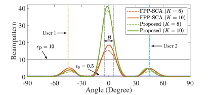
We first consider a transmit system with a uniform linear array of N=10𝑁10N=10 antennas and K=8𝐾8K=8 or 101010 RF chains. There are M=2𝑀2M=2 users located at 45superscript45-45^{\circ} and 45superscript4545^{\circ}. The mainlobe and sidelobe are =[5,5]superscript5superscript5\mathcal{B}=[-5^{\circ},5^{\circ}] and ¯=[90,60][30,20][20,30][60,90]¯superscript90superscript60superscript30superscript20superscript20superscript30superscript60superscript90\bar{\mathcal{B}}=[-90^{\circ},-60^{\circ}]\cup[-30^{\circ},-20^{\circ}]\cup[20^{\circ},30^{\circ}]\cup[60^{\circ},90^{\circ}]. The thresholds for the mainlobe and sidelobe response are ϵp=10subscriptitalic-ϵp10\epsilon_{{\mathrm{p}}}=10 and ϵs=0.5subscriptitalic-ϵs0.5\epsilon_{{\mathrm{s}}}=0.5. The maximum power radiated by each antenna is Pn=40dBmsubscript𝑃𝑛40dBmP_{n}=40~{}\text{dBm}, nfor-all𝑛\forall n, the same as [7]. The noise variance is set to σm2=1superscriptsubscript𝜎𝑚21\sigma_{m}^{2}=1, mfor-all𝑚\forall m. The threshold for the received SINR is γm=10dBsubscript𝛾𝑚10dB\gamma_{m}=10~{}\text{dB}, mfor-all𝑚\forall m. The number of constraints in Problem (13) is L=38𝐿38L=38, the tuning parameter is222We do not study the relationship between η𝜂\eta and the sparsity of the solution, because of the space limitation of the paper. Instead, when we obtain 𝐰^^𝐰{\bf{\widehat{w}}}, we choose K𝐾K antennas corresponding to the largest (in an 2,1subscript21\ell_{2,1}-norm sense) K𝐾K components. We have good results when the tuning parameter is η=0.1𝜂0.1\eta=0.1. η=0.1𝜂0.1\eta=0.1, and the augmented Lagrangian parameter is ρ=50𝜌50\rho=50 (ρ/2η/Lmuch-greater-than𝜌2𝜂𝐿\rho/2\gg\eta/L is satisfied). The value of 𝐯l(init)superscriptsubscript𝐯𝑙(init){\bf v}_{l}^{\text{(init)}} is given by any feasible point, while 𝐮l(init)=𝟎superscriptsubscript𝐮𝑙(init)0{\bf u}_{l}^{\text{(init)}}={\bf 0} and kmax=100subscript𝑘max100k_{\mathrm{max}}=100. The beampatterns are drawn in Fig. 2, which indicates that both the proposed and FPP-SCA methods have beamlobes in the radar mainlobe \mathcal{B} and the users directions. In addition, the proposed method has much higher response within \mathcal{B} than the FPP-SCA method.

Refer to caption

Figure 2: Beampattern comparison.

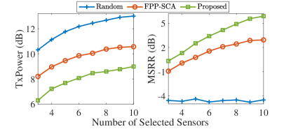
Next, we examine the TxPower and MSRR versus the number of selected sensors, i.e., K𝐾K. We also consider a strategy of randomly selecting K𝐾K sensors. The parameters are the same as those in the last example. 500500500 Monte-Carlo trials are performed. The results are plotted in Fig. 3. It is seen that our proposed method has the lowest transmit power and the highest MSRR, among all tested methods.
Refer to caption

Figure 3: TxPower (left) and MSRR (right) versus K𝐾K.

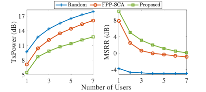
Finally, we test the TxPower and MSRR versus the number of users, i.e., M𝑀M. The number of selected antennas is fixed as K=8𝐾8K=8, and the other parameters are unchanged as in the last example. The results are depicted in Fig. 4, which again show that our algorithm leads to a more power-efficient solution.
Refer to caption

Figure 4: TxPower (left) and MSRR (right) versus M𝑀M.

V Conclusion

We studied the problem of sparse array design for dual-function radar-communications. Our design aimed at maintaining good control in both mainlobe and sidelobe, and also to keep the signal-to-interference-plus-noise ratio for the users larger than a certain level. In addition, we considered the limitation of the radiated power by each antenna. The problem was formulated as a quadratically constrained quadratic program, and solved by the consensus alternating direction method of multipliers. The proposed algorithm was able to be implemented in parallel. Simulation results demonstrated better performance of the proposed algorithm than the other tested methods.

Appendix A Proof of Theorem

Solving (27) is equal to finding a point in {𝐯l:𝐯lH𝐅l𝐯lfl}conditional-setsubscript𝐯𝑙superscriptsubscript𝐯𝑙Hsubscript𝐅𝑙subscript𝐯𝑙subscript𝑓𝑙\{\!{\bf v}_{l}\!:\!{\bf{v}}_{l}^{\mathrm{H}}{\bf F}_{l}{\bf{v}}_{l}\!\leq\!f_{l}\!\}, such that it is closest (in an 2subscript2\ell_{2}-norm sense) to 𝐯¯lsubscript¯𝐯𝑙{\bf{\bar{v}}}_{l}. Hence, the theorem equivalently states that the solution to Problem (15d) is the point closest (in an 2subscript2\ell_{2}-norm sense) to 𝐯¯lsubscript¯𝐯𝑙{\bf{\bar{v}}}_{l}, provided that ρ/2η/Lmuch-greater-than𝜌2𝜂𝐿{\rho}/{2}\gg{\eta}/{L}. To show this, we denote 𝐯~lsubscript~𝐯𝑙{\bf{\widetilde{v}}}_{l} as the point in {𝐯l:𝐯lH𝐅l𝐯lfl}conditional-setsubscript𝐯𝑙superscriptsubscript𝐯𝑙Hsubscript𝐅𝑙subscript𝐯𝑙subscript𝑓𝑙\{{\bf v}_{l}:{\bf{v}}_{l}^{\mathrm{H}}{\bf F}_{l}{\bf{v}}_{l}\leq f_{l}\}, such that

𝐯~l𝐯¯l2𝐯l𝐯¯l2subscriptnormsubscript~𝐯𝑙subscript¯𝐯𝑙2subscriptnormsubscript𝐯𝑙subscript¯𝐯𝑙2\displaystyle\|{\bf{\widetilde{v}}}_{l}-{\bf{\bar{v}}}_{l}\|_{2}\leq\|{\bf v}_{l}-{\bf{\bar{v}}}_{l}\|_{2} (28)

holds for any 𝐯l{𝐯l:𝐯lH𝐅l𝐯lfl}subscript𝐯𝑙conditional-setsubscript𝐯𝑙superscriptsubscript𝐯𝑙Hsubscript𝐅𝑙subscript𝐯𝑙subscript𝑓𝑙{\bf v}_{l}\in\{{\bf v}_{l}:{\bf{v}}_{l}^{\mathrm{H}}{\bf F}_{l}{\bf{v}}_{l}\leq f_{l}\}. Our goal is to show f(𝐯~l)f(𝐯l)𝑓subscript~𝐯𝑙𝑓subscript𝐯𝑙f({\bf{\widetilde{v}}}_{l})\leq f({\bf v}_{l}), for any 𝐯l{𝐯l:𝐯lH𝐅l𝐯lfl}subscript𝐯𝑙conditional-setsubscript𝐯𝑙superscriptsubscript𝐯𝑙Hsubscript𝐅𝑙subscript𝐯𝑙subscript𝑓𝑙{\bf v}_{l}\in\{{\bf v}_{l}:{\bf{v}}_{l}^{\mathrm{H}}{\bf F}_{l}{\bf{v}}_{l}\leq f_{l}\}.

The Lagrangian parameter ρ𝜌\rho is chosen as ρ=Cη/L𝜌𝐶𝜂𝐿\rho=C\eta/L, where C𝐶C is a constant. Then, |g(𝐯l)f(𝐯l)|0𝑔subscript𝐯𝑙𝑓subscript𝐯𝑙0|g({\bf v}_{l})-f({\bf v}_{l})|\to 0 as C𝐶C\to\infty (i.e., ρ/2η/Lmuch-greater-than𝜌2𝜂𝐿\rho/2\gg\eta/L), where g(𝐯l)ρ2𝐯l𝐰+𝐮l22𝑔subscript𝐯𝑙𝜌2superscriptsubscriptnormsubscript𝐯𝑙𝐰subscript𝐮𝑙22g({\bf v}_{l})\triangleq\frac{\rho}{2}\|{\bf v}_{l}-{\bf w}+{\bf u}_{l}\|_{2}^{2}. Moreover,

f(𝐯l)=g(𝐯l)=ρ2𝐯l𝐯¯l22,𝑓subscript𝐯𝑙𝑔subscript𝐯𝑙𝜌2superscriptsubscriptnormsubscript𝐯𝑙subscript¯𝐯𝑙22\displaystyle f({\bf v}_{l})=g({\bf v}_{l})=\frac{\rho}{2}\|{\bf v}_{l}-{\bf{\bar{v}}}_{l}\|_{2}^{2}, (29)

as long as C𝐶C\to\infty. Note that, in the second equality above, we used the fact that 𝐯¯l=𝐰𝐮lsubscript¯𝐯𝑙𝐰subscript𝐮𝑙{\bf{\bar{v}}}_{l}={\bf w}-{\bf u}_{l} as C𝐶C\to\infty.

Suppose that there exists a point 𝐯˘l{𝐯l:𝐯lH𝐅l𝐯lfl}subscript˘𝐯𝑙conditional-setsubscript𝐯𝑙superscriptsubscript𝐯𝑙Hsubscript𝐅𝑙subscript𝐯𝑙subscript𝑓𝑙{\bf{\breve{v}}}_{l}\in\{{\bf v}_{l}:{\bf{v}}_{l}^{\mathrm{H}}{\bf F}_{l}{\bf{v}}_{l}\leq f_{l}\}, such that f(𝐯˘l)<f(𝐯~l)𝑓subscript˘𝐯𝑙𝑓subscript~𝐯𝑙f({\bf{\breve{v}}}_{l})<f({\bf{\widetilde{v}}}_{l}). Thus, by using (29), we obtain that ρ2𝐯˘l𝐯¯l22<ρ2𝐯~l𝐯¯l22𝜌2superscriptsubscriptnormsubscript˘𝐯𝑙subscript¯𝐯𝑙22bra𝜌2subscript~𝐯𝑙evaluated-atsubscript¯𝐯𝑙22\frac{\rho}{2}\|{\bf{\breve{v}}}_{l}-{\bf{\bar{v}}}_{l}\|_{2}^{2}<\frac{\rho}{2}\|{\bf{\widetilde{v}}}_{l}-{\bf{\bar{v}}}_{l}\|_{2}^{2}, which contradicts (28). This implies that f(𝐯~l)f(𝐯l)𝑓subscript~𝐯𝑙𝑓subscript𝐯𝑙f({\bf{\widetilde{v}}}_{l})\leq f({\bf v}_{l}) holds for all feasible 𝐯lsubscript𝐯𝑙{\bf v}_{l}, that is, 𝐯~lsubscript~𝐯𝑙{\bf{\widetilde{v}}}_{l} is the solution to Problem (15d). This completes the proof.

References

  • [1] K. V. Mishra, B. Shankar, V. Koivunen, B. Ottersten, and S. A. Vorobyov, “Toward millimeter-wave joint radar communications: A signal processing perspective,” IEEE Signal Process. Mag., vol. 36, no. 5, pp. 100–114, Sep. 2019.
  • [2] F. Liu, C. Masouros, A. P. Petropulu, H. Griffiths, and L. Hanzo, “Joint radar and communication design: Applications, state-of-the-art, and the road ahead,” IEEE Trans. Commun., vol. 68, no. 6, pp. 3834–3862, Jun. 2020.
  • [3] S. Shi, Z. Cheng, L. Wu, Z. He, and B. Shankar, “Distributed 5G NR-based integrated sensing and communication systems: Frame structure and performance analysis,” in Proc. Eur. Signal Process. Conf. (EUSIPCO), Belgrade, Serbia, Aug. 2022, pp. 1062–1066.
  • [4] Z. Cheng, L. Wu, B. Wang, B. Shankar, B. Liao, and B. Ottersten, “Hybrid beamforming in mmWave dual-function radar-communication systems: Models, technologies, and challenges,” Oct. 2022. [Online]. Available: https://arxiv.org/abs/2209.04656
  • [5] C. Yang and H.-R. Shao, “WiFi-based indoor positioning,” IEEE Commun. Mag., vol. 53, no. 3, pp. 150–157, Mar. 2015.
  • [6] H. Wymeersch, G. Seco-Granados, G. Destino, D. Dardari, and F. Tufvesson, “5G mmWave positioning for vehicular networks,” IEEE Wirel. Commun., vol. 24, no. 6, pp. 80–86, Dec. 2017.
  • [7] E. Chen and M. Tao, “ADMM-based fast algorithm for multi-group multicast beamforming in large-scale wireless systems,” IEEE Trans. Commun., vol. 65, no. 6, pp. 2685–2698, Jun. 2017.
  • [8] A. M. Elbir, K. V. Mishra, B. Shankar, and B. Ottersten, “A family of deep learning architectures for channel estimation and hybrid beamforming in multi-carrier mm-Wave massive MIMO,” IEEE Trans. Cogn. Commun. Netw., vol. 8, no. 2, pp. 642–656, Jun. 2022.
  • [9] E. Raei, S. Sedighi, M. Alaee-Kerahroodi, and B. Shankar, “MIMO radar transmit beampattern shaping for spectrally dense environments,” IEEE Trans. Aerosp. Electron. Syst., pp. 1–13, Aug. 2022.
  • [10] A. Kassaw, D. Hailemariam, M. Fauß, and A. M. Zoubir, “Fractional programming for energy efficient power control in uplink massive MIMO systems,” in Proc. Eur. Signal Process. Conf. (EUSIPCO), A Coruna, Spain, Sep. 2019, pp. 1–5.
  • [11] S. A. Hamza and M. G. Amin, “Sparse array beamforming design for wideband signal models,” IEEE Trans. Aerosp. Electron. Syst., vol. 57, no. 2, pp. 1211–1226, Apr. 2021.
  • [12] T. Wei, L. Wu, and B. Shankar, “Sparse array beampattern synthesis via majorization-based ADMM,” in Proc. IEEE Veh. Technol. Conf. (VTC2021-Fall), Norman, USA, Sep. 2021, pp. 1–5.
  • [13] H. Huang, H. C. So, and A. M. Zoubir, “Sparse array beamformer design via ADMM,” Sep. 2022. [Online]. Available: https://arxiv.org/abs/2208.12313
  • [14] L. Wang, Q. He, and H. Li, “Transmitter selection and receiver placement for target parameter estimation in cooperative radar-communications system,” IET Signal Process., vol. 16, no. 7, pp. 776–787, Feb. 2022.
  • [15] Z. Xu, F. Liu, and A. P. Petropulu, “Cramér-Rao bound and antenna selection optimization for dual radar-communication design,” in Proc. IEEE Int. Conf. Acoust. Speech Signal Process. (ICASSP), Singapore, Singapore, May 2022, pp. 5168–5172.
  • [16] X. Zhang, X. Wang, and X. Wang, “Joint antenna selection and waveform design for coexistence of MIMO radar and communications,” EURASIP J. Adv. Signal Process., pp. 1–27, Dec. 2022.
  • [17] X. Wang, A. Hassanien, and M. G. Amin, “Sparse transmit array design for dual-function radar communications by antenna selection,” Digit. Signal Process., vol. 83, pp. 223–234, Dec. 2018.
  • [18] X. Wang, A. Hassanien, and M. G. Amin, “Dual-function MIMO radar communications system design via sparse array optimization,” IEEE Trans. Aerosp. Electron. Syst., vol. 55, no. 3, pp. 1213–1226, Jun. 2019.
  • [19] A. Ahmed, S. Zhang, and Y. D. Zhang, “Antenna selection strategy for transmit beamforming-based joint radar-communication system,” Digit. Signal Process., vol. 105, p. 102768, Oct. 2020.
  • [20] H. Huang, H. C. So, and A. M. Zoubir, “Off-grid direction-of-arrival estimation using second-order Taylor approximation,” Signal Process., vol. 196, p. 108513, Jul. 2022.
  • [21] K. Huang and N. D. Sidiropoulos, “Consensus-ADMM for general quadratically constrained quadratic programming,” IEEE Trans. Signal Process., vol. 64, no. 20, pp. 5297–5310, Oct. 2016.
  • [22] O. Mehanna, K. Huang, B. Gopalakrishnan, A. Konar, and N. D. Sidiropoulos, “Feasible point pursuit and successive approximation of non-convex QCQPs,” IEEE Signal Process. Lett., vol. 22, no. 7, pp. 804–808, Jul. 2015.