Physics-Informed Neural Networks for Prognostics and Health Management of Lithium-Ion Batteries

Abstract

For Prognostics and Health Management (PHM) of Lithium-ion (Li-ion) batteries, many models have been established to characterize their degradation process. The existing empirical or physical models can reveal important information regarding the degradation dynamics. However, there are no general and flexible methods to fuse the information represented by those models. Physics-Informed Neural Network (PINN) is an efficient tool to fuse empirical or physical dynamic models with data-driven models. To take full advantage of various information sources, we propose a model fusion scheme based on PINN. It is implemented by developing a semi-empirical semi-physical Partial Differential Equation (PDE) to model the degradation dynamics of Li-ion batteries. When there is little prior knowledge about the dynamics, we leverage the data-driven Deep Hidden Physics Model (DeepHPM) to discover the underlying governing dynamic models. The uncovered dynamics information is then fused with that mined by the surrogate neural network in the PINN framework. Moreover, an uncertainty-based adaptive weighting method is employed to balance the multiple learning tasks when training the PINN. The proposed methods are verified on a public dataset of Li-ion Phosphate (LFP)/graphite batteries.

I Introduction

Global sales of Electric Vehicles (EVs) doubled in 2021 from 2020 to a new record of 6.6 million according to [1] released by International Energy Agency (IEA). It keeps rising strongly and 2 million were sold in the first quarter of 2022, up 75% from the same period in the previous year. As their power source, Lithium-ion (Li-ion) batteries have become one of the most important industrial consumables. The demand for batteries reached 340 Gigawatt-hours (GWh) in 2021, which also doubled from the previous year. In the same year, the average battery price is USD 132/kWh. The cost of battery replacement due to its degradation is still high [2], and the Battery Management System (BMS) is developed to perform Prognostics and Health Management (PHM). The primary tasks of BMS include both State of Health (SoH) estimation and Remaining Useful Life (RUL) prognostics [3]. Fused usage information collected from various sources via BMS is expected to significantly improve the performance of PHM.

Generally, information fusion has been achieved in various flexible forms, including data-level , feature-level, decision-level, and model-level. The prognostic models can be categorized as physics-based models, experience-based models, and data-driven models [4, 5]. Physics-based and experience-based models represent abundant prior domain knowledge of the monitored systems condensed by experts that have been widely accepted [6]. There is no insurmountable gap between these two categories of models since many physics models originate from empirical models, such as the Paris–Erdogan equation. On the contrary, building data-driven models is a process of mining latent information in data. Dynamic models are commonly built to represent the governing dynamics during degrading, which can provide critical insights into the internal change of monitored systems.

According to the No-Free-Lunch (NFL) theorem, information from different models fits distinct problems well. Model fusion can leverage the advantages of combining the information from different categories of available models for PHM. It can be difficult to categorize fusion forms of model fusion. Five mostly-applied forms of fusing models are reviewed according to the combination and interfaces of distinct types of prognostic models [4]. Fusing physics-based models and data-driven PHM methods drags much attention [7]. Among these fusion forms, transition equations built based on physics or experience have been widely integrated into the framework of Bayesian filtering [8, 9]. These transition equations are then used to iterate the degradation state. This implementation of fusing physics-informed dynamic models and data-driven prognostic models inspires the frontiers of Physics-Informed Machine Learning (PIML) [10] in PHM.

The principle of PIML is to fuse the physics (experience)-based models and data-driven models. As reviewed in [4], this category of model fusion can be instantiated in various forms as well. Typical implementations of PIML are reviewed in [10] in terms of their applicable scenarios, principles, frameworks, and applications. As a formalized framework among PIML methods, Physics-Informed Neural Network (PINN) gains momentum since dynamic models established in various forms can be integrated. This high-level flexibility makes it popular in multiple frontiers such as epidemiology [11], power electronics [12, 13], acoustics [14], and electromagnetics [15]. For instance, [11] showed how PINN is capable of forecasting various highly-infectious diseases progression (e.g. COVID, HIV, and Ebola, etc.) whose spread can be modeled by Ordinary Differential Equations (ODEs) or Partial Differential Equations (PDEs). [12] monitored the parameter variations of a DC-DC Buck converter robustly and accurately based on a small training dataset of only 360 data samples with PINN. These concrete examples in different fields show the significance and generalizability of this method.

In this paper, we propose a semi-physics and semi-empirical dynamic model based on the Verhulst model [16] to capture the fading trends of the battery SoH. This model is further generalized as a PDE considering observable features given charging and discharging profiles, and a new parameter that represents the level of initial Solid Electrolyte Interphase (SEI) formation is introduced. To estimate the SoH of Li-ion batteries, we introduce PINN to fuse the prior information formulated as the dynamic model and the information extracted from monitoring data. Besides, a Deep Hidden Physics Model (DeepHPM) is also employed to discover the dynamics as a comparison with the improved Verhulst model for SoH estimation. It is also used for RUL prognostics without any explicit dynamic model. This implementation is a fusion of information mined by two data-driven models with different functions [4]. During the training of PINN, we use an uncertainty-based method to adaptively weigh the losses of subsequently proposed multi-task learning. The proposed methods are then verified on a public experimental cycling dataset of Li-ion Phosphate (LFP)/graphite batteries.

The contributions of this paper are threefold: 1) We propose a new scheme to seamlessly fuse prior information of physical or empirical degradation models and that of monitoring data in PHM for Li-ion batteries. 2) We propose a new semi-physical semi-empirical dynamic degradation to provide more insight into capacity loss. 3) We propose a scheme of fusing information of two distinct-designed data-driven models when there is little prior information. Moreover, the proposed models can be trained with an adaptive weighting method, which solves the challenge of combining losses appropriately in training PINNs. The code and data accompanying this paper are available on GitHub.

The rest of this article is organized as follows. Section II provides an overview of related work in terms of degradation modeling and the schemes of fusing dynamics in Deep Learning (DL). Section III setups the focused problem and the establishment of two categories of dynamic models is introduced, including an improved Verhulst model and DeepHPM-based automatically discovered models. Section IV presents the framework of PINN for model fusion and its training method, where an adaptively uncertainty-based multi-task balancing technique is included. Section V and VI verify the proposed methods on a public experimental dataset, and several details are provided in Appendix A. Finally, Section VII concludes this article.

II Related Work

II-A Dynamic Degradation Models of Li-Ion-Batteries

Dynamic models for Li-ion-batteries degradation can be established based on the classic Pseudo-Two-dimensional (P2D) model, which possesses high accuracy but is severely restricted due to the subsequent complexity and computation burden [17]. The Single-Particle (SP) model is then proposed to simplify the P2D model, which assumes that both electrodes consist of multiple uniform-sized spherical particles [18]. Based on the SP model, a widely-accepted degradation mechanism was proposed. Since electrolytes can be reduced in the presence of lithiated carbon, SEI formation is caused by the lithium carbonate. The newly exposed surface of the particles is then covered by SEI during the cycling. Under this mechanism, the degradation rate considering both Diffusion Induced Stresses (DIS), crack growth, and SEI thickness growth was derived in [19, 18]. There are many parameters to estimate and verify in this dynamic model proposed fully based on prior electrochemical knowledge, which restricts its generalizability.

Another category of degradation models focuses more on the utilization of available degradation data with monitoring time or cycles, and then the degradation trends are modeled by analytical functions under the given statistical assumptions [20]. These models commonly oversimplify the physics that the degradation trends of Li-ion batteries should follow. Semi-physics and semi-empirical dynamic models are proposed to take both factors into account [21]. For instance, an exponential-law model can be derived based on battery Coulombic efficiency [22]. This exponential model can also be integrated from an empirically given differential form and then its parameters are estimated based on temperature stress, State of Charge (SoC) stress, time stress, and Depth of Discharge (DoD) stress [21].

In view of the fact that there is an upper bound for the capacity loss, the Verhulst model has been proposed to quantify the rate of capacity loss [16]. As can be seen, there usually exists more or less available information from physics for SoH estimation, while this is not always true for RUL prognostics. To fill this gap, discovery for dynamic models with a preset fixed form or completely arbitrary form has been explored by developing PDE-Net [23, 24] and DeepHPM [25, 26] respectively. These models discover PDEs by training specialized layers. In PDE-Net, convolution kernels are trained to approximate the differential operators, and other network parameters are trained to approximate finite-order linear PDEs. Discrete-time models can be accordingly constructed. In DeepHPM, the most significant difference is that it uses the Automatic Differentiator (AutoDiff) to compute the analytical differentiation. As a result, DeepHPM can handle both discrete and continuous, linear and nonlinear models.

II-B Fusion of the Dynamics in Deep Learning

In the literature, several studies have been conducted integrating the dynamic models into DL, as follows.

Difference equations are the most commonly used discrete-time models. For example, temporal-modeling-specialized Recurrent Neural Network (RNN) and its variants can be applied to quantify the dynamics between different monitoring times by using a series of equations [27]. Several classic variants of RNN have fixed forms of these equations, such as the Long-Short Term Memory (LSTM) NN and the Gated Recurrent Unit (GRU) NN. Based on the domain knowledge of monitored systems, these equations can be re-designed to fuse prior physical information. Considering the cumulative damage of the grease and bearing damage, the physics of wind turbine main bearing fatigue was used to design a specific RNN cell for its PHM [28]. More physics including grease curves, bearing design data, and bearing design curves were further fused in their following work [29]. Since the RNN cell was completely reconstructed, these methods demand quite a deep understanding of the monitoring systems. Otherwise, these physics-informed cells may be inferior to the generic LSTM or GRU architectures.

Compared with these methods, the constraint learning scheme is more convenient to incorporate physical dynamics. It learns the knowledge by adding regularization that is determined by the physical constraints. For the inevitable calculation of differential terms in the dynamic models, approximating by the specially designed filters and AutoDiff are two general methods. For example, to approximate the spatial gradients in computer vision, the Sobel filter is an efficient approximator [30]. By contrast, PINN uses AutoDiff that can provide the exact partial derivatives. This scheme can handle both discrete and continuous time models.

When building the discrete-time models by using PINN, a multi-outputs NN is established where each neuron on the output layer outputs the predicted implicit intermediate states between two observable ones. These outputs are coupled and constrained in the framework of the implicit Runge-Kutta method during training [31, 12]. In this way, a priori-designed Butcher tableau is required given a certain number of the setup intermediate states coupled with a specific interval length between the two observable states [32]. On the contrary, an NN is established to directly approximate the implicit solution of the continuous time dynamic models.

In this paper, we focus on the continuous form of PINN to fuse the established dynamic models, which are provided by using the Verhulst model and the DeepHPM corresponding to the cases whether the prior domain knowledge is partially known or not at all.

III Problem Statement

Battery aging results from a combined action of both times went and cycling [21, 33]. Fading in a Li-ion battery upon charging and discharging can be attributed to a coupled mechanical-chemical degradation within the cell. The DISs can boost the growth of the cracks on the electrode surfaces during cycling and thus leading to the growth of SEI [18, 19]. This degradation mechanism assembles the fatigue process of materials upon cyclic loading [21], where the capacity loss due to the stress accumulates independently and ultimately causes life loss. Such a process can be categorized as cycle aging. At the same time, a battery also degrades over time because of the inherent slow electrochemical reaction, forming the calendar aging. Since charging and discharging processes can often be completed in dozens of minutes while calendar aging becomes observable usually on the scales of months or even years, cycle aging contributes the most to capacity and life loss. As a result, we assume that calendar aging can be neglected here when modeling the degradation dynamics of batteries.

The failure time of a Li-ion battery is commonly defined as the time when its currently usable capacity reduces below a pre-specified threshold [34]. SoH of a battery is consequently related to its current capacity and is typically defined as the ratio of current capacity over the nominal one [35]. Here we focus on the Percentage Capacity Loss (PCL) $u$ which represents the relative gap between the usable capacity and the nominal one, and it is denoted as:

$$u_{k}=1-SoH_{k}=1-\frac{Q_{k}}{Q_{Nom}}\times 100\%,$$ (1)

where $Q_{Nom}$ represents the nominal capacity and $Q_{k}$ represents the usable capacity in $k^{\mathrm{th}}$ cycle.

III-A Dynamic Models

Without loss of generality, PCL $u$ can be set as a uni-variate function of a virtual continuous independent time variable $t$ [36] whose unit is still the cycles. When a battery is operated upon identical conditions upon each cycle, a series of observations can be acquired at discrete time $t_{k}$:

$$u_{k}=u\left(t_{k}\right).$$ (2)

To handle the degradation dynamics of the battery degradation trend, the fading rate of its capacity can be denoted as

$$\frac{\mathrm{d}u\left(t\right)}{\mathrm{d}t}=\mathcal{G}\left(t,u;\Theta\right).$$ (3)

Eq. (3) is an explicit ODE parameterized by set $\Theta$, and $\mathcal{G}$ denotes a nonlinear function of $t$ and $u$. For instance, based on SEI formation and the growth process on both the initial and cracked surface [19, 18], eq. (3) can be specified as

$$\left.\frac{\mathrm{d}u\left(t\right)}{\mathrm{d}t}\right|_{t=t_{k}} =\theta_{1}\theta_{5}\left(1+\theta_{2}t_{k}\right)^{\frac{\theta_{3}}{2-\theta_{3}}}+\theta_{4}t_{k}^{-\frac{1}{2}},$$ (4)

$$+\theta_{1}\theta_{6}\sum_{l=1}^{k-1}\left[1+\theta_{2}\left(t_{k}-t_{l}\right)\right]^{\frac{\theta_{3}}{2-\theta_{3}}}\left(t_{k}-t_{l}\right)^{-\frac{1}{2}},$$

$$l <k,$$ (5)

where $t_{l}$ represents the monitoring time earlier than $t_{k}$ and $\Theta=\left\{\theta_{1},\theta_{2},\ldots,\theta_{6}\right\}$ are composite parameters. Each of them should be set according to dozens of electrochemical parameters including the geometric area of the graphite electrode film, the activation energy for crack propagation, and the solid phase porosity of the electrode film, etc. This theoretical model details molecular-level aging mechanism but it can be hardly employed in practical applications due to the lack of detailed cell conditions. Such a dynamic model describes a degradation trend reported in [37] with a decelerated trend of $u$ during the early cycles and a moderate linear trend [38] during the latter cycles. Based on the observed trend, a simplified semi-empirical model was proposed in [21] by using regression analysis:

$$\frac{\mathrm{d}u\left(t\right)}{\mathrm{d}t}=\theta\left[1-u\left(t\right)\right],$$ (6)

where $\theta$ denotes a basic linearized degradation rate that is co-determined by SoC, DoD, and cell temperature. An exponential-function solution with a decreasing absolute value of derivative can be acquired by integrating (6) to $u$. It can be observed that this model may not fit the battery degradation with an accelerated trend during the early cycles reported in [39, 40].

III-B Improved Verhulst Dynamic Model

Here the function $\mathcal{G}\left(t,u;\Theta\right)$ is also made dependent on the health state of the cell, and takes the simplest linear form as an instance:

$$\frac{\mathrm{d}u\left(t\right)}{\mathrm{d}t} =ru\left(t\right),$$ (7)

$$\mathrm{\mathit{s.t.}}\,\,u\left(t\right),\,r >0.$$

where $r$ is the degradation constant. Eq. (7) and partial term of (6) mark that the rate at which the capacity loss changes is proportional to the usable capacity at that time. The solution of (7) is the exponential function $u\left(t\right)=u_{0}\exp\left(rt\right)$ with an initial loss $u_{0}$, representing an accelerated degradation trend. This initial loss $u_{0}$ is commonly set as 10% [19]. Considering the capacity loss results from SEI growth and so on is always finite, a constant $K$ representing the upper bound of capacity loss is introduced to constrain the increasing rate of loss:

$$\frac{\mathrm{d}u\left(t\right)}{\mathrm{d}t} =ru\left(t\right)\left[1-\frac{u\left(t\right)}{K}\right],$$ (8)

$$\mathrm{s.t.}\,\,r >0,$$

$$0 <u\left(t\right)<K.$$

Eq. (8) is also known as the logistic differential equation proposed by Pierre Verhulst to model the population growth process [16]. When the lost capacity increases close to $K$, the increasing rate $\mathrm{d}u\left(t\right)/\mathrm{d}t$ will decline until it is close to 0. Since a battery is commonly considered as failed when its $u$ increases exceed 20%, it can be a priori roughly known that $K$ has a range of 20% to 100%. Furthermore, SEI will naturally form after a brand-new battery is manufactured and before use. In this process, the capacity loss caused by the SEI formation is supposed not to be governed by these dynamic models. Instead, a parameter $C$ that denotes such initial capacity loss is introduced to modify the model (8) as

$$\frac{\mathrm{d}u\left(t\right)}{\mathrm{d}t} =r\left[u\left(t\right)-C\right]\left[1-\frac{u\left(t\right)-C}{K-C}\right].$$ (9)

$$\mathrm{s.t.}\,\,r >0,$$

$$0 <u\left(t\right)<K,$$

$$0 <C\leq u_{0}.$$

Even though under identical operation conditions, different cells manufactured in the same batch may show distinct degradation characteristics. With the setup that $u$ is a uni-variate function of $t$, this cell-to-cell heterogeneity can be modeled by the difference in degradation model parameters [41, 42]. Considering the sole time-independent variable $t$ cannot distinguish specific trajectory when different batteries are fading, other variables that can indicate the latent health state can be introduced. In this setup, $u$ is expanded to a multi-variate function of both $\bm{x}=\left[x_{1},x_{2},\ldots,x_{S}\right]^{\mathrm{T}}\in\mathbb{R}^{S}$ and $t$. An $S$-dimensional Health Indicator (HI) $\bm{x}$ can characterize the health state during the battery fading, and both monitoring data and designed representative features can act as health indicators [38, 43]. It is feasible that cell-to-cell heterogeneity is quantified by different specific combinations of values in the feature space. The degradation rate given $\bm{x}$ and monitoring time $t$ is subsequently modeled by a PDE as:

$$\frac{\mathrm{\partial}u\left(\bm{x},t\right)}{\mathrm{\partial}t} =r\left[u\left(\bm{x},t\right)-C\right]\left[1-\frac{u\left(\bm{x},t\right)-C}{K-C}\right].$$ (10)

$$\mathrm{s.t.}\,\,r >0,$$

$$0 <u\left(t\right)<K,$$

$$0 <C\leq u_{0}.$$

The parameters of eq. (10) are of the same meanings as those in eq. (9).

III-C Data-Driven Dynamic Model

The dynamic model (10) depicts one of many forms of SoH degrading. Beyond SoH prognostics, it can be difficult to distill degradation mechanisms when predicting other variables such as RUL. Following (3), we define more generalized nonlinear dynamics parameterized by $\Theta$ to distill the mechanisms governing the evolution [25] of given data of HIs and time as

$$u_{t}-\mathcal{G}\left(\bm{x},t,u,u_{\bm{x}},u_{\bm{x}\bm{x}},u_{\bm{x}\bm{x}\bm{x}},\ldots;\Theta\right)=0.$$ (11)

In eq. (11), $u_{\bm{x}}=\left[\frac{\mathrm{\partial}u}{\mathrm{\partial}x_{1}},\frac{\mathrm{\partial}u}{\mathrm{\partial}x_{2}},\ldots,\frac{\mathrm{\partial}u}{\mathrm{\partial}x_{S}}\right]^{\mathrm{T}}$ denotes the first-order partial derivative of $u$ with respect to $\bm{x}$ and so on. The nonlinear function $\mathcal{G}$ poses more flexible relations on $t$, $u$, and their any-order partial derivatives. Subsequently, an infinite dimensional dynamical system can be represented by $\mathcal{G}$ [25]. As can be seen, (10) is a specific implementation of (11) where $\mathcal{G}\left(u;\Theta\right)=r\left(u-C\right)\left(1-\frac{u-C}{K-C}\right)$. In most cases of health monitoring, it is challenging to define an explicit dynamic model. With scattered and noisy monitoring observations, bias still exists in the PDE model (10) and the more-complicated latent dynamics. We construct a Neural Network (NN) as a function approximator [44] to fill this gap beyond a particular family of basis functions [26], forming a DeepHPM [25]:

$$u_{t}-\mathrm{DeepHPM}\left(\bm{x},t,u,u_{\bm{x}},u_{\bm{x}\bm{x}},u_{\bm{x}\bm{x}\bm{x}},\ldots;\Theta\right)=0.$$ (12)

Here we denote the NN used to approximate $\mathcal{G}$ as the DeepHPM. The parameter set $\Theta$ represents the trainable network parameters of the function approximator DeepHPM.

IV Methodology

The PDE dynamic model established based on prior knowledge (10) or approximated by NN (12) can be quite hard to solve. Based on the well-known capability of NNs as universal function approximators, we employ another NN parameterized by $\Phi$ to approximate the hidden solution $u\left(\bm{x},t;\Phi\right)$ of the system. Solution $u\left(\bm{x},t;\Phi\right)$ is also called the surrogate network. With this NN solver, the direct access or approximations to the involved partial derivatives are unnecessary [31, 25]. Model fusion of the surrogate NN with the explicit PDE models or DeepHPM formulates a PINN.

IV-A Model Fusion by PINN

A typical structure of PINN consists of three modules including a dynamic model, a surrogate NN, and an automatic differentiator. The dynamic model $\mathcal{G}\left(\bm{x},t,u,u_{\bm{x}},u_{\bm{x}\bm{x}},u_{\bm{x}\bm{x}\bm{x}},\ldots;\Theta\right)$ distills the mechanisms governing the dynamics of a degrading system, which can be either explicitly defined as (10) or approximated by a DeepHPM as (12). The surrogate NN $u\left(\bm{x},t;\Phi\right)$ is used to approximate the hidden solution $u\left(\bm{x},t\right)$ of the dynamic model, and the AutoDiff [45] is used to calculate values of all involved partial differentials input to the dynamic model.

Except for solving the latent $u\left(\bm{x},t\right)$ to build the prognostic model, discovering the dynamic model is realized by identifying the parameter set $\Theta$ of either specific PDE or DeepHPM. Identifying the unknown parameters forms a high-dimensional inverse problem describing the dynamical system. With the surrogate NN $u\left(\bm{x},t;\Phi\right)$, we define the left-hand side of eq. (12) as a function $f\left(\bm{x},t;\Phi,\Theta\right)$:

$$f\left(\bm{x},t;\Phi,\Theta\right)\coloneqq u_{t}\left(\bm{x},t;\Phi\right)-\mathcal{G}\left(\bm{x},t,u,u_{\bm{x}},u_{\bm{x}\bm{x}},u_{\bm{x}\bm{x}\bm{x}},\ldots;\Theta\right).$$ (13)

The parameters $\Phi$ of surrogate NN $u\left(\bm{x},t;\Phi\right)$ and $\Theta$ of dynamic model $\mathcal{G}\left(\bm{x},t,u,u_{\bm{x}},u_{\bm{x}\bm{x}},u_{\bm{x}\bm{x}\bm{x}},\ldots;\Theta\right)$ can be trained by minimizing the mean squared error losses:

$$\mathcal{L}=\lambda_{u}\mathcal{L}_{u}+\lambda_{f}\mathcal{L}_{f}+\lambda_{f_{t}}\mathcal{L}_{f_{t}},$$ (14)

where

$$\mathcal{L}_{u}= \sum_{i=1}^{N}\left[u\left(\bm{x}_{i},t_{i};\Phi\right)-u_{i}\right]^{2},$$ (15)

$$\mathcal{L}_{f}= \sum_{i=1}^{N}\left[f\left(\bm{x}_{i},t_{i};\Phi,\Theta\right)\right]^{2},$$ (16)

$$\mathcal{L}_{f_{t}}= \sum_{i=1}^{N}\left[f_{t}\left(\bm{x}_{i},t_{i};\Phi,\Theta\right)\right]^{2}.$$ (17)

Loss function (14) actually represents multi-task learning. Weight coefficients $\lambda_{u}$, $\lambda_{f}$, and $\lambda_{f_{t}}$ can be tuned to balance the loss terms in the training process. The loss term $\mathcal{L}_{u}$ corresponds to the regression fitting error at the collected observations, while $\mathcal{L}_{f}$ and $\mathcal{L}_{f_{t}}$ enforce the structure of PINN imposed by (11) and its first-order partial derivative with respect to $t$ [46]. Here $\mathcal{D}_{Train}=\left\{\bm{x}_{i},t_{i},u_{i}\right\}_{i=1}^{N}$ denotes the training data and $u_{i}$ represent the label to be predicted corresponding to the input data $\left\{\bm{x}_{i},t_{i}\right\}$, which can be actual SoH or RUL in PHM of batteries for the instance.

IV-B Framework of PINN

Figure 1: Framework of typical data-driven vanilla NN.

Figure 2: Framework of PINN-Verhulst.

Figure 3: Framework of PINN-DeepHPM.

Here the involved frameworks include a data-driven vanilla NN (baseline), a PINN with the Verhulst equation as the dynamic model (PINN-Verhulst), and a PINN with a DeepHPM as the dynamic model (PINN-DeepHPM). These frameworks are shown in Fig. 1, 2, and 3, respectively. To compare the respective learning framework clearer, the vanilla NN in the baseline is also denoted as a surrogate NN although there is no PDE to be solved. Since DeepHPM is used to discover the dynamic models when there are no available explicit dynamic models, it can be seen from Fig. 2 and 3 that those two frameworks are similar. The key difference is that the Verhulst model in Fig. 2 is then substituted as the DeepHPM in Fig. 3, and the corresponding partial derivatives input to the dynamic model are therefore substituted accordingly. It should be noted that these inputs are not fixed and need to be further selected in practice. Moreover, it is demonstrated that the proposed framework is flexible that can incorporate various forms of physical knowledge.

The basic structure of the surrogate NNs is illustrated in Fig. 4. The hidden layers of the surrogate NNs are all composed of Fully Connected (FC) layers, and the hyperbolic tangent is employed as the activation function due to its differentiability. Structures of all the involved surrogate NNs in both Fig. 1, 2, and 3 are set as this if there are no special notes. The structure of DeepHPM is set the same as that of the surrogate NNs.

Figure 4: Basic structure of NNs.

IV-C Weight Coefficients Tuning in Training PINN

Focusing on the loss function (14) of training a PINN, it can be observed that PINN is constrained or regularized by the loss imposed by the given set of PDEs beyond a regression task at the given data set. It is observed that networks are sensitive to the relative weights of multiple objective functions from desired training tasks [47]. Manually tuning the weighting coefficients $\lambda$ can be quite expensive, and methods for adaptive tuning during the training are desirable. Numerical stiffness will cause unbalanced back-propagated gradients in the PINN training process, and the weighting coefficients can be accordingly tuned based on the gradient statistics [48]. Other mechanisms have also been utilized to design the adaptive balancing such as random lookback [49] and homoscedastic aleatoric uncertainty [47]. Following [47], the likelihood of the observed data labels is assumed as Gaussian. The mean of likelihood is set as the output of the surrogate NNs and the variance is set according to the weighting coefficient:

$$p\left(\left.\bm{u}\right|u\left(\bm{X},\bm{t};\Phi\right)\right)=\mathcal{N}\left(u\left(\bm{X},\bm{t};\Phi\right),\frac{1}{\lambda_{u}}\right),$$ (18)

where $\bm{u}=\left[u_{1},u_{2},\ldots,u_{N}\right]^{\mathrm{T}}$, $\bm{X}=\left[\bm{x}_{1},\bm{x}_{2},\ldots,\bm{x}_{N}\right]^{\mathrm{T}}$, and $\bm{t}=\left[t_{1},t_{2},\ldots,t_{N}\right]^{\mathrm{T}}$ consist of labels and samples of the training set respectively. The output corresponding to the loss $\mathcal{L}_{u}$ is used as the instance and the other objectives in (14) can be accordingly defined. The observation noise scalar is set related to the weighting coefficient $\lambda$ corresponding to the output in the loss function. The log-likelihood can be written as

$$\log p\left(\left.\bm{u}\right|u\left(\bm{X},\bm{t};\Phi\right)\right)\propto-\frac{\lambda_{u}}{2}\left\|\bm{u}-u\left(\bm{X},\bm{t};\Phi\right)\right\|^{2}+\frac{1}{2}\log\lambda_{u}.$$ (19)

Based on (15), (16), (17), and (19), the multi-task minus log-likelihood can be obtained as (20).

$$-\log p\left(\left.\bm{u},\bm{f},\bm{f}_{t}\right|u\left(\bm{X},\bm{t};\Phi\right),f\left(\bm{X},\bm{t};\Phi,\Theta\right)\right)$$

$$= -\log\left[p\left(\left.\bm{u}\right|u\left(\bm{X},\bm{t};\Phi\right)\right)\cdot p\left(\left.\bm{f}\right|f\left(\bm{X},\bm{t};\Phi,\Theta\right)\right)\cdot p\left(\left.\bm{f}_{t}\right|f\left(\bm{X},\bm{t};\Phi,\Theta\right)\right)\right],$$

$$= -\log p\left(\left.\bm{u}\right|u\left(\bm{X},\bm{t};\Phi\right)\right)-\log p\left(\left.\bm{f}\right|f\left(\bm{X},\bm{t};\Phi,\Theta\right)\right)-\log p\left(\left.\bm{f}_{t}\right|f\left(\bm{X},\bm{t};\Phi,\Theta\right)\right),$$

$$= \lambda_{u}\left\|\bm{u}-u\left(\bm{X},\bm{t};\Phi\right)\right\|^{2}+\lambda_{f}\left\|\bm{f}-f\left(\bm{X},\bm{t};\Phi,\Theta\right)\right\|^{2}+\lambda_{f_{t}}\left\|\bm{f}_{t}-f_{t}\left(\bm{X},\bm{t};\Phi,\Theta\right)\right\|^{2}-\log\lambda_{u}\lambda_{f}\lambda_{f_{t}},$$

$$= \lambda_{u}\mathcal{L}_{u}+\lambda_{f}\mathcal{L}_{f}+\lambda_{f_{t}}\mathcal{L}_{f_{t}}-\log\lambda_{u}\lambda_{f}\lambda_{f_{t}}.$$ (20)

It can be seen that the loss function (14) is regularized as:

$$\mathcal{L}=\lambda_{u}\mathcal{L}_{u}+\lambda_{f}\mathcal{L}_{f}+\lambda_{f_{t}}\mathcal{L}_{f_{t}}-\log\lambda_{u}\lambda_{f}\lambda_{f_{t}}.$$ (21)

With these settings, relative weighting coefficients $\lambda_{u}$, $\lambda_{f}$, and $\lambda_{f_{t}}$ of the loss terms can be learned by minimizing the regularized loss function (21) adaptively. The output weighted noise is constrained by the penalty term $\log\lambda_{u}\lambda_{f}\lambda_{f_{t}}$. In practice, we define $\lambda^{\prime}\coloneqq-\log\lambda$ and train $\lambda^{\prime}$ for numerical stability. The loss function (21) can be subsequently rewritten as:

$$\mathcal{L} =\exp\left(-\lambda^{\prime}_{u}\right)\mathcal{L}_{u}+\exp\left(-\lambda^{\prime}_{f}\right)\mathcal{L}_{f}+\exp\left(-\lambda^{\prime}_{f_{t}}\right)\mathcal{L}_{f_{t}}$$

$$+\lambda^{\prime}_{u}+\lambda^{\prime}_{f}+\lambda^{\prime}_{f_{t}}.$$ (22)

Training PINN by minimizing (22) instead of (14) is expected to balance the multiple losses, which is denoted as AdpBal here. The training process is summarized in Algorithm 1, where $\mathrm{SSE}\left(\cdot\right)$ represents computing Sum of Squares Error (SSE) by using eq. (15), (16), and (17), respectively. The dynamic model $\mathcal{G}\left(\cdot\right)$ can represent the explicit PDEs or that approximated by the DeepHPM.

Algorithm 1 Training proposed models.
Input: training data $\mathcal{D}=\left\{\bm{X},\bm{t},\bm{u}\right\}$, hyper-parameters.
Output: surrogate NN $u\left(\bm{X},\bm{t};\Phi\right)$, dynamic model $\mathcal{G}\left(\bm{X},\bm{t},\bm{u},\bm{u}_{\bm{x}},\bm{u}_{\bm{x}\bm{x}},\bm{u}_{\bm{x}\bm{x}\bm{x}},\ldots;\Theta\right)$.
1: initialize $\Phi$, $\Theta$, $\lambda^{\prime}_{u}$, $\lambda^{\prime}_{f}$, $\lambda^{\prime}_{f_{t}}$
2: for $epoch=1,2,\cdots$ do:
3:     $\hat{\bm{u}}\leftarrow u\left(\bm{X},\bm{t};\Phi\right)$
4:     $\hat{\bm{u}}_{t}\leftarrow\mathrm{AutoDiff}\left(\hat{\bm{u}},\bm{t}\right)$
5:     $\hat{\bm{u}}_{\bm{x}}\leftarrow\mathrm{AutoDiff}\left(\hat{\bm{u}},\bm{X}\right)$
6:     $\hat{\bm{u}}_{\bm{xx}}\leftarrow\mathrm{AutoDiff}\left(\hat{\bm{u}}_{\bm{x}},\bm{X}\right)$
7:     $\cdots$
8:     $\hat{\mathcal{G}}\leftarrow\mathcal{G}\left(\bm{X},\bm{t},\hat{\bm{u}},\hat{\bm{u}}_{\bm{x}},\hat{\bm{u}}_{\bm{xx}},\hat{\bm{u}}_{\bm{xxx}},\ldots;\Theta\right)$
9:     $\hat{\bm{f}}\leftarrow\hat{\bm{u}}_{t}-\hat{\mathcal{G}}$
10:     $\hat{\bm{f}}_{t}\leftarrow\mathrm{AutoDiff}\left(\hat{\bm{f}},\bm{t}\right)$
11:     $\mathcal{\hat{L}}_{u}\leftarrow\mathrm{SSE}\left(\hat{\bm{u}},\bm{u}\right)$
12:     $\mathcal{\hat{L}}_{f}\leftarrow\mathrm{SSE}\left(\hat{\bm{f}},\bm{0}\right)$
13:     $\mathcal{\hat{L}}_{f_{t}}\leftarrow\mathrm{SSE}\left(\hat{\bm{f}}_{t},\mathbf{0}\right)$
14:     compute loss $\hat{\mathcal{L}}$ by using eq. (22)
15:     update $\Phi$, $\Theta$, $\lambda^{\prime}_{u}$, $\lambda^{\prime}_{f}$, $\lambda^{\prime}_{f_{t}}$ on loss $\hat{\mathcal{L}}$
16: end

V Dataset Description and Preprocessing

V-A Dataset Description

The dataset involved in this paper consists of three batches of commercial LFP/graphite battery cells manufactured by A123 Systems, where a total of 124 cells were cycled to failure under dozens of different fast-charging protocols [40]. The nominal capacity of the cells is 1.1 Ah, and the unit charging and discharging rate 1C equals 1.1 A subsequently. Each charging protocol is marked as a string formatted as “C1(Q1)-C2”, where the corresponding cell was first charged with the current C1 from 0% SoC (unit: %) to the SoC Q1. When charged at Q1, the charging current was then switched to C2 with which the cell was charged to 80% SoC. All cells were finally charged from 80% to 100% SoC with a Constant-Current Constant-Voltage (CC-CV) form to the 3.6V upper cutoff potential and the C/50 cutoff current. Moreover, all cells were discharged also with a CC-CV form at 4C to 2.0V lower cutoff potential and the C/50 cutoff current. Detailed information on the studied cells and the experimental settings can be accessed in [40].

V-B Feature Extraction

Figure 5: Extracted features of cell #124.

Figure 6: SoH estimation of cell #124 in case A.

Figure 7: SoH estimation of cell #116 in case B.

As introduced in Section III and IV, appropriately designed health features $\bm{x}=\left[x_{1},x_{2},\ldots,x_{S}\right]^{\mathrm{T}}$ can effectively characterize the exact degradation process that each cell undergoes. Extracting features varying to the number of cycles for which the battery has operated attracts much attention. A critical principle is that the extracted features are expected to be of strong correlation with SoH [35]. Point features can be simply extracted based on the charging/discharging profiles during cycling, such as the peaks of Incremental Capacity (IC) curves during the CC charging [50]. Point features can be conveniently extracted mainly characterizing the transient state in each cycle. Interval features can represent characteristics in a period, and they can also be easily extracted by intercepting values on the profiles at certain intervals. Therefore, information related to SoH may be over-simplified since only values on the endpoints of the intervals are paid attention to. Interval features can be extracted as the charge time during the CC charging [39] and time intervals of equispaced charge current/voltage changing [51, 52] for the instance. To capture the trend variation of charging/discharging profiles during cycling, trend features are designed focusing on parameters varying upon a specific prior function modeling the profiles during a cycle. The trend of charging current during CV charging is approximately exponential, and the parameter of the fitted exponential function can be used as a trend feature [50]. Within a certain range of discharging voltage, differences in discharging capacity show a quadratic-function-formed trend to discharging capacity. Parameters of the quadratic polynomial can be accordingly estimated as the trend feature as well [35]. Other statistical features computed based on the whole profile of a cycle can also be employed such as the mean [53, 35], energy [54], Skewness [54], and Kurtosis [54], etc.

Following [35], we also extracted the trend feature based on the quadratic model:

$$Q_{i+1}\left(V_{i+1}\right)-Q_{i}\left(V_{i}\right)=-\omega\left[Q_{i}\left(V_{i}\right)\right]^{2}+b+\varepsilon.$$ (23)

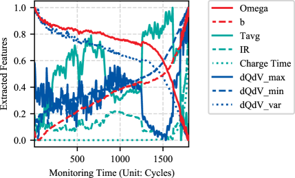
Eq. (23) is defined for the profile of each cycle. $Q_{i}\left(V_{i}\right)$ is a measurement of the discharging capacity with respect to the discharging voltage between 2.7V and 3.3V, and $\varepsilon\sim\mathcal{N}\left(0,\sigma^{2}\right)$ represents the normal measuring error. Undetermined coefficients $\omega$ and $b$ are estimated as two features in that cycle. Maximum, minimum, and the variance of the IC curve when the discharging voltage is between 2.7V and 3.3V are also used as features. Other employed features include average temperature, internal resistance, and charging time. To reduce the measurement noise, the moving average is then applied to the extracted features for better representative capability. All the extracted features from cell #124 are illustrated in Fig. 5 as an example, and it should be noted that the features are 0-1 normalized in this figure for better illustration.

V-C Standardization

Note that there are significant variations among different channels of inputs and outputs, which may severely impact the performance. Standardization is consequently implemented. The derivatives of outputs to the inputs can be kept unchanged in this way when using AutoDiff, and the standardized data are processed by the NN. On the other hand, the partial derivatives of the before- or after-standardization outputs to the before- or after-standardization inputs can be obtained. Here we employ the widely-used z-score standardization to scale inputs. Specifically, the standardization factors are set as the corresponding mean and standard deviation calculated from the training data:

$$\widetilde{x}_{i} =\frac{x_{i}-\mathrm{Mean}\left(\bm{X}_{Train}\right)}{\mathrm{Std}\left(\bm{X}_{Train}\right)},$$ (24)

$$\widetilde{u}_{i} =\frac{u_{i}-\mathrm{Mean}\left(\bm{u}_{Train}\right)}{\mathrm{Std}\left(\bm{u}_{Train}\right)}.$$ (25)

In eq. (24) and (25), $\bm{u}=\left[u_{1},u_{2},\ldots,u_{N}\right]^{\mathrm{T}}$ and $\bm{X}=\left[\bm{x}_{1},\bm{x}_{2},\ldots,\bm{x}_{N}\right]^{\mathrm{T}}$ consist of labels and samples of the training set as denoted in Section IV-C. Monitoring time $t$ is also standardized in this way since it can be regarded as part of inputs.

VI Case Study

Table I: General settings for training NNs

Settings	Values
Optimizer	Adam
Training epochs	2000 (Case A & B) / 8000 (Case C)
Learning rate	0.001
Batch size	1024 (Case A & B) / 8192 (Case C)
Initialization	Xavier Normal
Dropout probability	0.2

The proposed prognostic framework is verified for both SoH estimation and RUL prediction. For better comparison with the existing methods, the training set and test set are formed in different ways, which are marked as cases A, B, and C respectively. In case A, data from cells #91 and #100 are used for training/validation and cell #124 is used as the test set [35]. Their charging protocol is 4.36C(80%)-4.36C. In case B, data from cells #101, #108, and #120 are used for training/validation and cell #116 is used as the test set [35]. Their charging protocol follows 5.3C(54%)-4C. In case C, data from batch 2 are selected and 20% of them are randomly chosen as the test set [53]. These cells follow various charging protocols.

Here the widely used Root Mean Square Error (RMSE) metric is adopted to measure the performance. RMSE is formulated as:

$$\mathrm{RMSE}=\sqrt{\frac{1}{N}\sum_{i=1}^{N}\left(\hat{u}_{i}-u_{i}\right)^{2}},$$ (26)

where $\hat{u}_{i}$ and $u_{i}$ denote the output of the prediction model and the actual data label corresponding to $i^{\mathrm{th}}$ input sample. When it is used for SoH estimation, the output PCL should be transformed as SoH based on eq. (1). There are a total of $N$ samples in the test set. Moreover, we also adopt the Root Mean Square Percentage Error (RMSPE) as the metric since the scale of SoH and RUL can be quite distinct. RMSPE is formulated as:

$$\mathrm{RMSPE}=\sqrt{\frac{1}{N}\sum_{i=1}^{N}\left(\frac{\hat{u}_{i}-u_{i}}{u_{i}}\right)^{2}}\times 100\%.$$ (27)

Table II: Optimal settings for each case

Settings	SoH Estimation		RUL Prognostics
	Case A	Case B	Case A	Case B	Case C
No. of Layers	2	2	2	2	4
Neurons / Layer	128	64	128	128	128
DeepHPM inputs	$\bm{x},t$	$t$	$\bm{x},t,u$	$t,u,u_{\bm{x}}$	$t$

Figure 8: Variation of relative weighting coefficients by using adaptive balancing in the model training. (a)~(e) Respective variation of relative weighting coefficients in each round.

Division of training and test data have been detailed above. Then 20% of training-validation data are divided as the validation data in cases A and B, and 25% of training-validation data are divided as the validation data in case C. The rest of the training-validation data is used for training ultimately. Several general settings are listed in Table I. Other critical hyper-parameters such as the number of hidden layers and neurons are further tuned depending on the performance of validation data. To reduce the number of hyper-parameters to be tuned, we tune them based on baseline models as far as possible. Then the obtained optimal parameters for the baseline models are applied to the proposed models. It is worth mentioning that those parameters may not be the optima for the proposed models. For instance, optimal network structures (the number of hidden layers and neurons) are determined based on the vanilla data-driven NN illustrated in Fig. 1, and then they are used for both PINN-Verhulst and PINN-DeepHPM. It has been revealed that the performance of discovering dynamics by using DeepHPM can be sensitive to input terms [25, 23, 24], so which terms should be involved needs to be further explored. We organize various combinations of input features, monitoring time as well as partial derivatives to them as a candidate library. Similarly, simply summing the multiple losses in eq. (14) for training PINNs is further set as a baseline. The optimal combination of input terms in the library for DeepHPM is determined with this baseline, and then it is used to validate AdpBal for the multiple losses. Calculated RMSPEs for SoH estimation and RMSEs for RUL prognostics on the validation set in terms of the number of hidden layers and neurons per layer are listed in Tables VI, VII, VIII, IX, and X in the Appendix. Validation RMSPEs and RMSEs in terms of the combinations of inputs to DeepHPM are listed in Table XI. Accordingly, settings for different cases are determined and summarized in Table II. With these settings, the proposed models are all trained in a regular computation environment (Intel Xeon E5-2630 CPU, 2.2 GHz; Nvidia GeForce GTX 1080 Ti GPU). The training-test process is repeated for 5 rounds in each case, and the results are averaged to reduce the randomness.

Table III: Summarized results and the comparison for SoH estimation in cases A and B

Cases	GPR	GPR	Baseline	PINN-Verhulst	PINN-Verhulst	PINN-DeepHPM	PINN-DeepHPM
		(Onboard)		(Sum)	(AdpBal)	(Sum)	(AdpBal)
Case A	0.76	0.69	0.42	1.41	0.49	0.43	0.47
Case B	0.63	0.57	0.56	0.56	0.44	0.51	0.42

VI-A SoH Estimation

The two categories of dynamic models, the Verhulst model, and DeepHPM are used to estimate the SoH. This represents two cases that whether there are available explicit dynamic models respectively. The results of SoH estimation are summarized in Table III.

In case A, the calculated RMSPEs of SoH estimation on the validation data in terms of different combinations of the number of hidden layers and neurons are listed in Table VI. The optimal network structure for the data-driven baseline model is 2 hidden layers and 128 neurons per hidden layer. With this setting, the baseline model provides a 0.42% estimation error in terms of RMSPE on the test data. PINN-Verhulst provides a 1.41%-RMSPE estimation when simply summing the multiple losses. With AdpBal for tuning the weight coefficients of the losses, a 0.49% RMSPE can be obtained. When there is no prior explicit dynamic model, the inputs of DeepHPM are set as $\bm{x},t$ when discovering the dynamic model via DeepHPM according to Table XI. These validation errors are calculated by simply summing the multiple losses. the estimation errors are 0.43% and 0.47% respectively without and with AdpBal.

In case B, the network structure is set as 2 hidden layers with 64 neurons per hidden layer according to Table VII. With this setting, the baseline estimation error is 0.56%. PINN-Verhulst (Sum), PINN-Verhulst (AdpBal), PINN-DeepHPM (Sum), and PINN-DeepHPM (AdpBal) provide 0.56%, 0.44%, 0.51%, and 0.42% estimation errors in terms of RMSPEs.

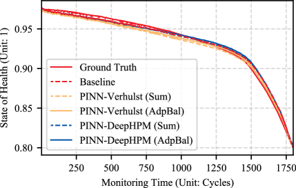
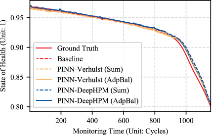
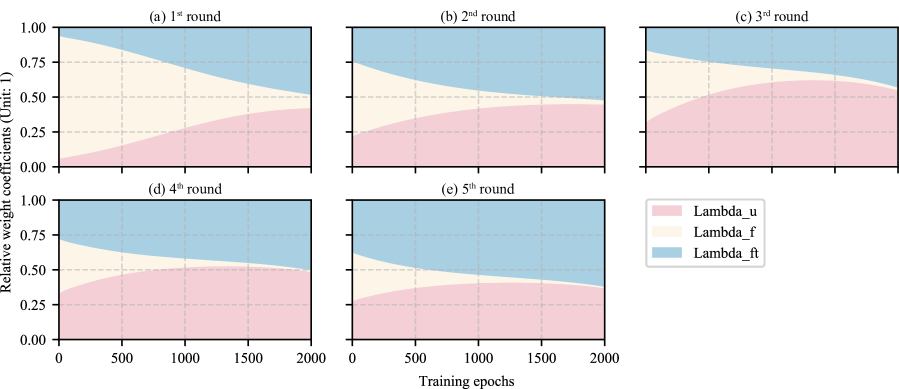
The SoH estimation is further illustrated in Fig. 6 and 7. The data-driven baseline method without model fusion can perform satisfactorily for SoH estimation, especially in case A. With fusing the improved Verhulst model, the performance of simply summing the losses has no significant improvement over the baseline. The estimation accuracy is even significantly declined in case A. By using the AdpBal, the performance is improved instead. Compared with case A, there is a better improvement in case B. The reason can be that the numbers of hidden layers and neurons are optimal for baseline, but probably not for the proposed methods. When DeepHPM is used to discover the governing dynamics, similar results are observed. It verifies the ability of DeepHPM to discover dynamics and the robustness of using AdpBal for training PINN. With AdpBal, relative values of the weighting coefficients changing in terms of the training epochs of case B in all 5 rounds are illustrated in Fig. 8. It can be seen that relative values of the weighting coefficients vary in similar ways during different rounds of training. This also shows the robustness of AdpBal. The average training time of the baseline data-driven model, PINN-Verhulst, and PINN-DeepHPM in case B are 87.6s, 122.7s, and 126.0s respectively. Moreover, the proposed methods are compared with a Gaussian Process Regression (GPR)-based method [35]. It is worth mentioning that partial onboard test data are further used to calibrate this GPR-based method (GPR Onboard) in [35]. It should be noted that the results of the methods compared here are directly quoted from the corresponding papers. This comparison is shown in Table III. As can be seen, the proposed methods perform better than this comparative study even without using any onboard test data.

Figure 9: RUL prognostics of cell #124 in case A.

Figure 10: RUL prognostics of cell #116 in case B.

VI-B RUL Prognostics

Table IV: Summarized results and the comparison for RUL prognostics in cases A and B

Cases	GPR	Baseline	PINN-DeepHPM	PINN-DeepHPM
			(Sum)	(AdpBal)
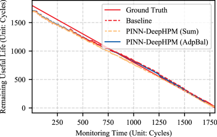
Case A	93.27	46.38	48.81	45.86
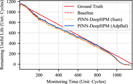
Case B	64.06	64.48	65.52	56.29

Table V: Summarized results and the comparison for RUL prognostics in case C

Cases	LSTM	Heteroscedastic	Homoscedastic	Bayesian	Bayesian DL	Baseline	PINN-DeepHPM	PINN-DeepHPM
		Bayesian LSTM	Bayesian LSTM	VAE-LSTM	(Calibration)		(Sum)	(AdpBal)
Case C	15.8	20.7	22.4	22.4	15.2	15.2	14.2	17.9

Since there is no prior explicit dynamic PDE model correlating the predicted RUL to the input features as well as monitoring time, only DeepHPM is employed here to discover the dynamics. The results are summarized in Tables IV and V.

Predicted and actual RUL of the test cells #124 and #116 are illustrated in Fig. 9 and 10. In case A, the data-driven prognostic model provides a 46.38 cycles error in terms of RMSE. With physics-informed losses based on the discovery of DeepHPM, the prediction error is 48.81 cycles. After AdpBal is turned on, the predictive RMSE is 45.86 cycles. The prognostic error is slightly reduced by 6.04% ((45.86$-$48.81)/48.81$\times$100%) after weighting coefficients are tuned automatically. In case B, the prediction RMSE of baseline, PINN-DeepHPM (Sum), and PINN-DeepHPM (AdpBal) are 64.48, 65.52, and 56.29 cycles respectively. The prognostic error is significantly reduced by 14.09% ((56.29$-$65.52)/65.52$\times$100%) after weighting coefficients are tuned automatically. Similar to that of SoH estimation, the proposed method shows a minor improvement in case A and a major improvement in case B. As a result, the generalizability of the proposed methods from SoH estimation to RUL prognostics is verified. In case C, RUL prognostics error is reduced by 6.7% ((14.19$-$15.21)/15.21$\times$100%) with introducing DeepHPM. However, the performance deteriorated by using AdpBal. A possible reason can be that there are multiple operation conditions for the cells in case C, which severely impacts the homoscedastic uncertainty among measurements of cells. Moreover, the proposed methods are compared with an LSTM NN, a Heteroscedastic Bayesian LSTM, a Homoscedastic Bayesian LSTM, a Bayesian VAE-LSTM, and a Bayesian DL framework incorporating uncertainty quantification and calibration [53]. It can be seen from Table V that the fused PINN-DeepHPM outperforms those LSTM-based methods. LSTM commonly fits temporal information better than vanilla NN since it can capture the dynamics by using differential equations. The fusion with DeepHPM enables the vanilla NN to capture the dynamics as well.

VI-C Discussion

In the PHM of Li-ion batteries, electrochemical models with higher complexity may provide better estimations, such as the SP models. However, the methods to specify the model parameters need further development since the automatic discovery of parameters can be challenging in that case. In this paper, only the vanilla NN is used to construct the PINN. The performance may be seriously limited due to the simple structure of the vanilla NN. On the other hand, there is still a lack of research on how more powerful architectures of NNs, such as the RNN, the Convolutional Neural Network (CNN), and their variants, will affect the propagation and differentiation in PINN. For example, these advanced network structures can relate a single output $u_{k}$ to multiple inputs $\left(\bm{x}_{i},t_{i}\right),\,i=1,2,\cdots,N$ in the time domain. This modification will profoundly affect the dynamic model (11) since all partial differentials will vary with the monitoring time in this equation. As a result, more theoretical research needs to be conducted to fill this critical gap.

VII Conclusion

In this article, we propose a new model fusion framework for Li-ion batteries PHM based on PINN. A flexible form is provided by PINN to fuse empirical or physical dynamic models and data-driven surrogate NNs. With the established dynamic model, the rate of capacity degrading can be quantified with respect to the operating cycles and the current SoH of monitored cells. The generalization of the dynamic model to a PDE form fits different cells with the same combination of parameters. The added extra parameter can represent the initial SEI formation, which is a common reason for capacity loss in the initial cycles. Under this setting, the model is more consistent with the physical characteristics of battery degradation. DeepHPM provides a specialized model to discover the governing dynamics of battery degradation when lacking prior information. With the uncertainty-based weighting method, losses of multiple learning tasks can be adaptively balanced when training the PINN. Implementation of a public dataset verifies the effectiveness of the proposed methods. The results show that the proposed model fusion scheme can improve the performance of PHM for Li-ion batteries, but an appropriate weighting method is compulsory to balance the multi-task losses for training PINN.

In future directions, special attention should be paid to the issues of possible failure to learn complex physical phenomena for general implementations of PINN. To enhance the performance of PINN, more efforts can be spent on improving the convergence, stability, boundary conditions, network design, and optimization [55]. How to propagate the gradients along the temporal dimension in RNN or spatial dimension in CNN and their variants can be quite a potential direction. Another possible direction together with this issue is how to integrate the temporal or spatial gradients into the PDEs.

Appendix A Performance of Different Settings on the Validation Data

A-A NN Structures for SoH Estimation

In terms of the different number of hidden layers and neurons per layer, the calculated RMSPEs for SoH estimation on the validation set in respective cases are listed in Tables VI and VII. These results are calculated by using the vanilla NN (Baseline).

Table VI: Validation RMSPE with respect to the number of hidden layers and neurons per layer in Case A based on the baseline model (Unit: %)

	8	16	32	64	128
2	2.4e-01	1.4e-01	1.0e-01	8.9e-02	7.9e-02
4	3.7e-01	2.2e-01	1.5e-01	1.2e-01	1.5e-01
6	5.0e-01	2.7e-01	1.9e-01	1.6e-01	2.0e-01
8	6.4e-01	3.3e-01	2.2e-01	2.0e-01	2.0e-01
10	8.3e-01	5.1e-01	4.1e-01	2.7e-01	2.4e-01

Table VII: Validation RMSPE with respect to the number of hidden layers and neurons per layer in Case B based on the baseline model (Unit: %)

	8	16	32	64	128
2	2.7e-01	1.8e-01	1.4e-01	1.1e-01	1.1e-01
4	4.0e-01	2.5e-01	1.8e-01	1.7e-01	1.7e-01
6	4.4e-01	3.2e-01	2.3e-01	1.9e-01	2.2e-01
8	5.1e-01	3.5e-01	2.5e-01	2.3e-01	2.3e-01
10	6.2e-01	5.4e-01	3.8e-01	2.8e-01	2.8e-01

A-B NN Structures for RUL Prognostics

In terms of the different number of hidden layers and neurons per layer, calculated RMSEs for RUL prognostics on the validation set in respective cases are listed in Tables VIII, IX, and X. These results are calculated by using the vanilla NN (Baseline).

Table VIII: Validation RMSE with respect to the number of hidden layers and neurons per layer in Case A based on the baseline model (Unit: Cycles)

	8	16	32	64	128
2	29.45	19.82	13.26	10.39	8.31
4	50.32	29.55	20.65	15.50	15.32
6	58.56	42.38	24.00	21.43	21.65
8	63.49	48.25	29.05	24.96	22.06
10	68.40	51.97	38.42	26.44	25.57

Table IX: Validation RMSE with respect to the number of hidden layers and neurons per layer in Case B based on the baseline model (Unit: Cycles)

	8	16	32	64	128
2	35.75	23.67	17.12	14.81	12.73
4	44.52	27.59	20.27	15.31	14.55
6	50.79	30.14	24.22	18.06	17.40
8	56.89	41.24	28.29	20.41	16.63
10	62.02	40.63	34.08	21.15	17.19

Table X: Validation RMSE with respect to the number of hidden layers and neurons per layer in Case C based on the baseline model (Unit: Cycles)

	8	16	32	64	128
2	107.02	77.33	53.88	35.50	23.38
4	113.65	77.40	46.75	23.31	14.92
6	119.27	81.05	48.38	23.99	15.02
8	129.26	87.30	54.36	27.59	15.26
10	144.46	95.78	58.84	29.97	17.00

Table XI: Validation metrics with respect to the combinations of inputs of DeepHPM based on the PINN-DeepHPM with simply summing losses (Unit: % for SoH estimation; Cycles for RUL prognostics)

DeepHPM Inputs	SoH Estimation		RUL Prognostics
	Case A	Case B	Case A	Case B	Case C
$\bm{x}$	9.7e-02	1.1e-01	9.17	11.70	15.52
$t$	9.7e-02	1.1e-01	9.13	12.02	14.05
$u$	1.6e-01	2.7e-01	9.13	12.02	14.07
$u_{\bm{x}}$	2.6e-01	2.9e-01	9.17	11.70	26.00
$\bm{x},t$	7.9e-02	1.1e-01	8.76	12.16	15.04
$\bm{x},u$	1.9e-01	2.1e-01	8.76	12.16	15.04
$\bm{x},u_{\bm{x}}$	2.6e-01	3.2e-01	8.80	12.38	23.35
$t,u$	2.2e-01	1.9e-01	9.11	11.89	15.18
$t,u_{\bm{x}}$	2.5e-01	2.7e-01	8.75	12.16	26.59
$u,u_{\bm{x}}$	2.6e-01	3.2e-01	8.76	12.17	28.29
$\bm{x},t,u$	1.8e-01	2.1e-01	8.40	11.69	15.90
$\bm{x},t,u_{\bm{x}}$	2.5e-01	2.8e-01	8.97	12.36	21.99
$\bm{x},u,u_{\bm{x}}$	2.7e-01	2.9e-01	8.96	12.34	24.40
$t,u,u_{\bm{x}}$	3.0e-01	2.9e-01	8.41	11.68	22.77
$\bm{x},t,u,u_{\bm{x}}$	2.8e-01	2.7e-01	9.31	11.71	24.98

A-C Combinations of Inputs of DeepHPM

In terms of the different combinations of inputs to the DeepHPM, calculated metrics on the validation set in respective cases are listed in Table XI. With the NN structures that are determined according to Appendices A-A and A-B, these results are calculated by using the PINN-DeepHPM by simply summing the losses (Sum).

Pengfei Wen (S’20) received B.S. and Ph.D. degrees in Information and Communication Engineering from the School of Electronics and Information, Northwestern Polytechnical University (NWPU), Xi’an, China, in 2017 and 2023, respectively. From 2021 to 2022, he was a Visiting Ph.D. Student with the Department of Industrial Systems Engineering and Management, National University of Singapore, Singapore, with the scholarship from NWPU and Huawei Technologies Co., Ltd. His current research interests include Information Fusion, Reliability Engineering, and Physics-Informed Machine Learning.

Zhi-Sheng Ye (Senior Member, IEEE) received the joint B.E. degree in material science & engineering and in economics from Tsinghua University, Beijing, China, in 2008, and the Ph.D. degree in industrial and systems engineering from the National University of Singapore, Singapore, in 2012. He is currently an Associate Professor with the Department of Industrial Systems Engineering and Management, National University of Singapore. His research interests include reliability engineering, complex systems modeling, and industrial statistics.

Yong Li received the B.S. degree in Avionics Engineering, M.S. and Ph.D degrees in Circuits and Systems from Northwestern Polytechnical University, Xi’an, China, in 1983, 1988 and 2005, respectively. He joined School of Electronic Information, Northwestern Polytechnical University in 1993 and was promoted to professor in 2002. His research interests include digital signal processing and radar signal processing.

Shaowei Chen (M’15) is currently an associate professor in the School of Electronics and Information, Northwestern Polytechnical University, Xi’an, China, where he is also the dean of the Department of telcommunication engineering and the Director of Perception and IoT Information Processing Laboratory. He is the principal investigator of several projects supported by the Aeronautical Science Foundation of China, Beijing, China. His research expertise is in the area of the fault diagnosis, sensors, condition monitoring, and prognosis of electronic systems. Prof. Chen is selected to receive several Provincial and Ministerial Science and Technology Awards. He is a senior member of the Chinese Institute of Electronics.

Pu Xie obtained his PhD in the Department of Mechanical Engineering at Tsinghua University in 2016. After graduation, he joined CRRC Changchun Railway Vehicles Co., Ltd., where he conducted experimental research on structural fatigue and crack behavior using the MTS system. Currently, he is a visiting postdoctoral scholar in the Department of Aeronautics & Astronautics at Stanford University. His research interests are focused on developing and implementing advanced testing and diagnostic methods that enhance the safety and reliability of mechanical systems, as well as developing multiphysics analytical methods for solving complex problems.

Shuai Zhao (S’14-M’18) received the B.S., M.S., and Ph.D. degrees in information and telecommunication engineering from Northwestern Polytechnical University, Xi’an, China, in 2011, 2014, and 2018, respectively. He is currently an Assistant Professor with AAU Energy, Aalborg University, Denmark. From 2014 to 2016, he was a Visiting Ph.D. student with the Department of Mechanical and Industrial Engineering, University of Toronto, Canada. In August 2018, he was a Visiting Scholar with the Power Electronics and Drives Laboratory, Department of Electrical and Computer Science, University of Texas at Dallas, Richardson, TX, USA. From 2018 to 2022, he was a Postdoc researcher with AAU Energy, Aalborg University, Denmark. His research interests include physics-informed machine learning, system informatics, condition monitoring, diagnostics and prognostics, and tailored AI tools for power electronic systems.

References

- [1] E. M. Bibra, E. Connelly, S. Dhir, M. Drtil, P. Henriot, I. Hwang, J.-B. Le Marois, S. McBain, L. Paoli, and J. Teter, “Global EV outlook 2022: Securing supplies for an electric future,” Int. Energy Agency, Report, 2022.
- [2] Z. Wei, Y. Li, and L. Cai, “Electric vehicle charging scheme for a park-and-charge system considering battery degradation costs,” IEEE Trans. Intell. Veh., vol. 3, no. 3, pp. 361–373, 2018.
- [3] S. Schaut, E. Arnold, and O. Sawodny, “Predictive thermal management for an electric vehicle powertrain,” IEEE Trans. Intell. Veh., vol. 8, no. 2, pp. 1957–1970, 2023.
- [4] L. X. Liao and F. Kottig, “Review of hybrid prognostics approaches for remaining useful life prediction of engineered systems, and an application to battery life prediction,” IEEE Trans. Rel., vol. 63, no. 1, pp. 191–207, 2014.
- [5] S. Zhao, S. Chen, F. Yang, E. Ugur, B. Akin, and H. Wang, “A composite failure precursor for condition monitoring and remaining useful life prediction of discrete power devices,” IEEE Trans. Ind. Informat., vol. 17, no. 1, pp. 688–698, 2020.
- [6] K. Sarrafan, K. M. Muttaqi, and D. Sutanto, “Real-time state-of-charge tracking embedded in the advanced driver assistance system of electric vehicles,” IEEE Trans. Intell. Veh., vol. 5, no. 3, pp. 497–507, 2020.
- [7] M. Pecht, T. Shibutani, M. Kang, M. Hodkiewicz, and E. Cripps, “A fusion prognostics-based qualification test methodology for microelectronic products,” Microelectron. Rel., vol. 63, pp. 320–324, 2016.
- [8] L. Liao and F. Koettig, “A hybrid framework combining data-driven and model-based methods for system remaining useful life prediction,” Appl. Soft Comput., vol. 44, pp. 191–199, 2016.
- [9] Y. Z. Zhang, R. Xiong, H. W. He, and M. Pecht, “Validation and verification of a hybrid method for remaining useful life prediction of lithium-ion batteries,” J. Cleaner Prod., vol. 212, pp. 240–249, 2019.
- [10] G. E. Karniadakis, I. G. Kevrekidis, L. Lu, P. Perdikaris, S. F. Wang, and L. Yang, “Physics-informed machine learning,” Nat. Rev. Phys., vol. 3, no. 6, pp. 422–440, 2021.
- [11] S. Shaier, M. Raissi, and P. Seshaiyer, “Data-driven approaches for predicting spread of infectious diseases through DINNs: Disease informed neural networks,” Preprint arXiv:2110.05445v2, 2021.
- [12] S. Zhao, Y. Peng, Y. Zhang, and H. Wang, “Parameter estimation of power electronic converters with physics-informed machine learning,” IEEE Trans. Power Electron., vol. 37, no. 10, pp. 11 567–11 578, 2022.
- [13] S. Zhao, F. Blaabjerg, and H. Wang, “An overview of artificial intelligence applications for power electronics,” IEEE Trans. Power Electron., vol. 36, no. 4, pp. 4633–4658, 2020.
- [14] H. Y. Sun, L. S. Peng, J. M. Lin, S. Wang, W. Zhao, and S. L. Huang, “Microcrack defect quantification using a focusing high-order SH guided wave EMAT: The physics-informed deep neural network GuwNet,” IEEE Trans. Ind. Informat., vol. 18, no. 5, pp. 3235–3247, 2022.
- [15] H. Y. Sun, L. S. Peng, S. L. Huang, S. S. Li, Y. Long, S. Wang, and W. Zhao, “Development of a physics-informed doubly fed cross-residual deep neural network for high-precision magnetic flux leakage defect size estimation,” IEEE Trans. Ind. Informat., vol. 18, no. 3, pp. 1629–1640, 2022.
- [16] W. Xian, B. Long, M. Li, and H. Wang, “Prognostics of lithium-ion batteries based on the verhulst model, particle swarm optimization and particle filter,” IEEE Trans. Instrum. Meas., vol. 63, no. 1, pp. 2–17, 2013.
- [17] A. Jokar, B. Rajabloo, M. Désilets, and M. Lacroix, “Review of simplified pseudo-two-dimensional models of lithium-ion batteries,” J. Power Sour., vol. 327, pp. 44–55, 2016.
- [18] J. Li, K. Adewuyi, N. Lotfi, R. G. Landers, and J. Park, “A single particle model with chemical/mechanical degradation physics for lithium ion battery State of Health (SOH) estimation,” Appl. Energy, vol. 212, pp. 1178–1190, 2018.
- [19] R. Deshpande, M. Verbrugge, Y.-T. Cheng, J. Wang, and P. Liu, “Battery cycle life prediction with coupled chemical degradation and fatigue mechanics,” J. Electrochem. Soc., vol. 159, no. 10, p. A1730, 2012.
- [20] J.-Z. Kong, D. Wang, T. Yan, J. Zhu, and X. Zhang, “Accelerated stress factors based nonlinear wiener process model for lithium-ion battery prognostics,” IEEE Trans. Ind. Electron., vol. 69, no. 11, pp. 11 665–11 674, 2021.
- [21] B. Xu, A. Oudalov, A. Ulbig, G. Andersson, and D. S. Kirschen, “Modeling of lithium-ion battery degradation for cell life assessment,” IEEE Trans. Smart Grid, vol. 9, no. 2, pp. 1131–1140, 2018.
- [22] F. Yang, X. Song, G. Dong, and K.-L. Tsui, “A coulombic efficiency-based model for prognostics and health estimation of lithium-ion batteries,” Energy, vol. 171, pp. 1173–1182, 2019.
- [23] Z. Long, Y. Lu, X. Ma, and B. Dong, “PDE-Net: Learning PDEs from data,” in Int. Conf. Mach. Learn. PMLR, 2018, Conference Proceedings, pp. 3208–3216.
- [24] Z. Long, Y. Lu, and B. Dong, “PDE-Net 2.0: Learning PDEs from data with a numeric-symbolic hybrid deep network,” J. Comput. Phys., vol. 399, p. 108925, 2019.
- [25] M. Raissi, “Deep hidden physics models: Deep learning of nonlinear partial differential equations,” J. Mach. Learn. Res., vol. 19, pp. 932–955, 2018.
- [26] S. Cofre-Martel, E. L. Droguett, and M. Modarres, “Remaining useful life estimation through deep learning partial differential equation models: A framework for degradation dynamics interpretation using latent variables,” Shock Vib., vol. 2021, p. 9937846, 2021.
- [27] A. Sherstinsky, “Deriving the recurrent neural network definition and RNN unrolling using signal processing,” in CRACT Workshop at NeurIPS-2018, vol. 31, 2018, Conference Proceedings, p. 4.
- [28] Y. Yucesan and F. Viana, “A physics-informed neural network for wind turbine main bearing fatigue,” Int. J. Prognostics Health Manag., vol. 11, no. 1, p. 17, 2020.
- [29] Y. A. Yucesan and F. A. C. Viana, “Hybrid physics-informed neural networks for main bearing fatigue prognosis with visual grease inspection,” Comput. Ind., vol. 125, p. 103386, 2021.
- [30] Y. Zhu, N. Zabaras, P. S. Koutsourelakis, and P. Perdikaris, “Physics-constrained deep learning for high-dimensional surrogate modeling and uncertainty quantification without labeled data,” J. Comput. Phys., vol. 394, pp. 56–81, 2019.
- [31] M. Raissi, P. Perdikaris, and G. E. Karniadakis, “Physics-informed neural networks: A deep learning framework for solving forward and inverse problems involving nonlinear partial differential equations,” J. Comput. Phys., vol. 378, pp. 686–707, 2019.
- [32] A. Iserles, A first course in the numerical analysis of differential equations. Cambridge Univ. Press, 2009.
- [33] J. Shi, A. Rivera, and D. Wu, “Battery health management using physics-informed machine learning: Online degradation modeling and remaining useful life prediction,” Mech. Syst. Signal Process., vol. 179, p. 109347, 2022.
- [34] W. D. Connor, Y. Q. Wang, A. A. Malikopoulos, S. G. Advani, and A. K. Prasad, “Impact of connectivity on energy consumption and battery life for electric vehicles,” IEEE Trans. Intell. Veh., vol. 6, no. 1, pp. 14–23, 2021.
- [35] J. Kong, F. Yang, X. Zhang, E. Pan, Z. Peng, and D. Wang, “Voltage-temperature health feature extraction to improve prognostics and health management of lithium-ion batteries,” Energy, vol. 223, p. 120114, 2021.
- [36] Z. Liu, G. Sun, S. Bu, J. Han, X. Tang, and M. Pecht, “Particle learning framework for estimating the remaining useful life of lithium-ion batteries,” IEEE Trans. Instrum. Meas., vol. 66, no. 2, pp. 280–293, 2017.
- [37] R. Spotnitz, “Simulation of capacity fade in lithium-ion batteries,” J. Power Sour., vol. 113, no. 1, pp. 72–80, 2003.
- [38] P. Wen, S. Zhao, S. Chen, and Y. Li, “A generalized remaining useful life prediction method for complex systems based on composite health indicator,” Rel. Eng. Syst. Safety, vol. 205, p. 107241, 2021.
- [39] H. N. Liu, I. H. Naqvi, F. J. Li, C. L. Liu, N. Shafiei, Y. L. Li, and M. Pecht, “An analytical model for the CC-CV charge of Li-ion batteries with application to degradation analysis,” J. Energy Storage, vol. 29, p. 101342, 2020.
- [40] K. A. Severson, P. M. Attia, N. Jin, N. Perkins, B. Jiang, Z. Yang, M. H. Chen, M. Aykol, P. K. Herring, D. Fraggedakis, M. Z. Bazant, S. J. Harris, W. C. Chueh, and R. D. Braatz, “Data-driven prediction of battery cycle life before capacity degradation,” Nat. Energy, vol. 4, no. 5, pp. 383–391, 2019.
- [41] S. Zhao, Y. Peng, F. Yang, E. Ugur, B. Akin, and H. Wang, “Health state estimation and remaining useful life prediction of power devices subject to noisy and aperiodic condition monitoring,” IEEE Trans. Instrum. Meas., vol. 70, pp. 1–16, 2021.
- [42] K. Liu, N. Z. Gebraeel, and J. Shi, “A data-level fusion model for developing composite health indices for degradation modeling and prognostic analysis,” IEEE Trans. Autom. Sci. Eng., vol. 10, no. 3, pp. 652–664, 2013.
- [43] P. Wen, Y. Li, S. Chen, and S. Zhao, “Remaining useful life prediction of iiot-enabled complex industrial systems with hybrid fusion of multiple information sources,” IEEE Internet Things J., vol. 8, no. 11, pp. 9045–9058, 2021.
- [44] K. Hornik, M. Stinchcombe, and H. White, “Multilayer feedforward networks are universal approximators,” Neural Netw., vol. 2, no. 5, pp. 359–366, 1989.
- [45] A. G. Baydin, B. A. Pearlmutter, A. A. Radul, and J. M. Siskind, “Automatic differentiation in machine learning: a survey,” J. Mach. Learn. Res., vol. 18, pp. 1–43, 2018.
- [46] J. Yu, L. Lu, X. Meng, and G. E. Karniadakis, “Gradient-enhanced physics-informed neural networks for forward and inverse pde problems,” Comput. Methods Appl. Mech. Eng., vol. 393, p. 114823, 2022.
- [47] A. Kendall, Y. Gal, and R. Cipolla, “Multi-task learning using uncertainty to weigh losses for scene geometry and semantics,” in Proc. IEEE Conf. Comput. Vision Pattern Recognit., 2018, Conference Proceedings, pp. 7482–7491.
- [48] S. F. Wang, Y. J. Teng, and P. Perdikaris, “Understanding and mitigating gradient flow pathologies in physics-informed neural networks,” SIAM J. Scientific Comput., vol. 43, no. 5, pp. A3055–A3081, 2021.
- [49] R. Bischof and M. Kraus, “Multi-objective loss balancing for physics-informed deep learning,” arXiv preprint: 2110.09813, 2021.
- [50] G. Dong, W. Han, and Y. Wang, “Dynamic bayesian network-based lithium-ion battery health prognosis for electric vehicles,” IEEE Trans. Ind. Electron., vol. 68, no. 11, pp. 10 949–10 958, 2020.
- [51] Y. Ji, Z. Chen, Y. Shen, K. Yang, Y. Wang, and J. Cui, “An RUL prediction approach for lithium-ion battery based on SADE-MESN,” Appl. Soft Comput., vol. 104, p. 107195, 2021.
- [52] S. Pepe, J. P. Liu, E. Quattrocchi, and F. Ciucci, “Neural ordinary differential equations and recurrent neural networks for predicting the state of health of batteries,” J. Energy Storage, vol. 50, p. 104209, 2022.
- [53] Y.-H. Lin and G.-H. Li, “A bayesian deep learning framework for RUL prediction incorporating uncertainty quantification and calibration,” IEEE Trans. Ind. Informat., vol. 18, no. 10, pp. 7274–7284, 2022.
- [54] M. A. Patil, P. Tagade, K. S. Hariharan, S. M. Kolake, T. Song, T. Yeo, and S. Doo, “A novel multistage support vector machine based approach for Li ion battery remaining useful life estimation,” Appl. Energy, vol. 159, pp. 285–297, 2015.
- [55] S. Cuomo, V. S. Di Cola, F. Giampaolo, G. Rozza, M. Raissi, and F. Piccialli, “Scientific machine learning through physics-informed neural networks: Where we are and what’s next,” J. Sci. Comput., vol. 92, no. 3, p. 88, 2022.
![[Uncaptioned image]](/html/2301.00776/assets/x7.png) |