ENGNN: A General Edge-Update Empowered GNN Architecture for Radio Resource Management in Wireless Networks

Abstract

In order to achieve high data rate and ubiquitous connectivity in future wireless networks, a key task is to efficiently manage the radio resource by judicious beamforming and power allocation. Unfortunately, the iterative nature of the commonly applied optimization-based algorithms cannot meet the low latency requirements due to the high computational complexity. For real-time implementations, deep learning-based approaches, especially the graph neural networks (GNNs), have been demonstrated with good scalability and generalization performance due to the permutation equivariance (PE) property. However, the current architectures are only equipped with the node-update mechanism, which prohibits the applications to a more general setup, where the unknown variables are also defined on the graph edges. To fill this gap, we propose an edge-update mechanism, which enables GNNs to handle both node and edge variables and prove its PE property with respect to both transmitters and receivers. Simulation results on typical radio resource management problems demonstrate that the proposed method achieves higher sum rate but with much shorter computation time than state-of-the-art methods and generalizes well on different numbers of base stations and users, different noise variances, interference levels, and transmit power budgets.

I Introduction

Efficient radio resource management plays a vital role in achieving high data rate and ubiquitous connectivity of future wireless networks. In particular, beamforming design and power allocation have been recognized as crucial components to improve the spectrum/energy efficiency in ultra-dense networks[1], cloud radio access networks [2, 3], and cell-free massive multiple-input multiple-output systems [4].

Mathematically, many of the radio resource management problems belong to the challenging non-convex optimization problems, which are conventionally solved by numerical algorithms with a lot of iterations [5, 6]. However, due to the fast variation of the wireless environment, the iterative nature of the commonly applied optimization-based numerical algorithms cannot satisfy the low-latency requirement in beyond 5G paradigm. For instance, to maximize the sum rate of a multi-cell wireless system under the maximum transmit power constraint of each base station (BS), the conventional first-order algorithm, e.g., the gradient projection (GP) method [7], requires a lot of iterations to converge to a stationary point. To improve the convergence rate, while more advanced numerical algorithms such as the weighted minimum mean-square error (WMMSE) [8] algorithm can be applied, the matrix inverse in each iteration still makes it computationally expensive and hence difficult for the real-time implementation.

To facilitate the real-time implementation, deep learning based methods have become popular for radio resource management [9, 10, 11, 12, 13, 14, 15, 16]. Specifically, deep learning based methods utilize neural networks to learn a mapping function from many problem features to the corresponding solutions. Once the neural network is well trained, it can infer the solution of any new setting using simple feed-forward computations, and thus is extremely fast.

Inspired by the successful applications in computer vision, the multi-layer perceptrons (MLPs) and convolutional neural networks (CNNs) have been applied as typical architectures for representing the mapping functions in radio resource management. For example, MLPs were used to learn the mapping function from the wireless channel to the optimal resource management policy [9]. Moreover, an MLP-based architecture was adopted to learn the optimal power control for the multi-user interference channels [10]. Similarly, CNNs have also been applied for power control [11] and beamforming design [12] in the multiple-input single-output downlink systems. However, since MLPs and CNNs cannot fully exploit the topology in the wireless networks, they usually require a large number of training samples while still result in limited performance. For instance, it is shown in [16] that a CNN trained on a two-user wireless networks can only achieve the near-optimal performance for two-user wireless networks during the testing phase, but its performance degrades by $18\%$ in ten-user networks compared to the conventional optimization-based numerical algorithms.

Recently, attempts to use graph neural networks (GNNs) are on the rise because of their ability to exploit the topology of wireless networks. By modeling a wireless network as a graph, the known system parameters can be modeled as the graph features, which are treated as the input of a GNN, while the unknown variables to be optimized can also be defined on the graph and are served as the output of a GNN. The advantage of graph modeling lies in its permutation equivariance (PE) property, where the graph features/variables can be regarded as a set of elements whose index order does not matter. Consequently, a large number of unnecessary permuted training samples can be discarded [17, 18, 19]. Moreover, since the trainable parameters of GNNs are independent of the graph size, the well-trained GNNs can generalize well to different problem dimensions [20, 21, 22, 23, 24].

Among the existing GNN-based works, homogeneous GNNs, which share the trainable parameters among different graph nodes, have shown their good scalability and generalization performance for the radio resource management problems when there is only one type of graph nodes [17, 18, 19, 20, 24, 25, 26, 27, 28]. For example, in [17], a homogeneous GNN named message passing graph neural network (MPGNN) was proposed for beamforming design in the multi-transceiver interference channels, where each transceiver pair is modeled as an individual graph node. By modeling different transceiver pairs as the same type of nodes and sharing their trainable parameters, the test performance in terms of sum rate is near optimal even when the number of transceiver pair is twice larger than that in the training samples. Similarly, homogeneous GNNs have also been demonstrated to generalize well on different numbers of users in multicast beamforming design [24], link scheduling [25], power control [26, 27], and joint beam selection and link activation [28].

While homogeneous GNNs have shown their great success when there exists only one type of graph nodes in the radio resource management problems, it should be noticed that the more common scenarios usually consist of different types of graph nodes. For instance, in a general wireless network, the transmitters and receivers have different physical characteristics, and hence should be more naturally modeled as two different types of graph nodes, i.e., TX-nodes and RX-nodes. By sharing the trainable parameters within only the same type of nodes, heterogeneous GNNs [29] have shown their superiority for the more complex radio resource management problems compared with the homogeneous GNNs [30, 31, 32, 33, 34]. In particular, the pioneer work [30] designed a heterogeneous GNN called permutation equivariant heterogeneous GNN (PGNN) for the power allocation in multi-cell downlink systems, and theoretically established the PE property with respect to different user equipments (UEs) within each cell and also with respect to different cells. Moreover, heterogeneous GNNs have also been proposed for the beamforming design in heterogeneous device-to-device networks [31] and multi-user downlink systems [32]. In [33], a heterogeneous GNN was designed for jointly learning the beamforming vectors and reflecting phases for an intelligent reflecting surfaces (IRS) assisted multi-user downlink system, where the users and the IRS are modeled as heterogeneous graph nodes. Similarly, the trajectory of unmanned aerial vehicles (UAVs) was cooperatively designed by modeling the UAVs and the ground terminals as heterogeneous graph nodes in [34].

Despite the successes of the homogeneous or heterogeneous GNNs in the above existing works, they are only equipped with the node-update mechanism, which restricts the output of the neural networks, i.e., the unknown variables to be optimized only appear on the graph nodes. Notable examples are MPGNN [17] and PGNN [30], both of which do not consider the variables on the graph edges. In particular, MPGNN is proposed for the beamforming design for the multi-transceiver interference channels, where each transmitter only serves a single receiver. Therefore, each transceiver pair can be modeled as a single node, and the channel state information of each direct communication link serves as the corresponding node features. Furthermore, the interference links among different transceiver pairs are modeled as graph edges, whose channel state information is treated as the corresponding edge features. Using this graph model, the beamforming variable of each transceiver pair can be defined only on the corresponding node. On the other hand, PGNN is proposed for the power allocation in multi-cell systems, where each BS serves multiple UEs within the same cell. In this scenario, each BS adopts a pre-designed beamformer, so that a dedicated equivalent single-antenna channel is created for each UE. Consequently, with each equivalent transmit antenna treated as an individual node, the power allocation variables can also be defined on the graph nodes.

While all the above pioneering works exemplify the benefits of GNNs in radio resource management, currently applied architectures prohibit the extension to a more general setting, where the unknown variables are also defined on the graph edges. A typical application scenario is the cooperative beamforming design, where each transmitter serves multiple receivers, while each receiver is also served by multiple transmitters. These complicated transceiver interactions cannot be easily modeled by the current GNN architectures that are only equipped with the node-update mechanism. In fact, for the more general wireless environment, an individual beamforming or power variable belongs to a transceiver pair, which is represented by two different nodes. Thus, beamformers or power variables should be more naturally defined on the graph edges. Unfortunately, without a judiciously designed edge-update mechanism, the current widely adopted GNN architectures cannot handle such a general setting.

To fill this gap, we propose a novel edge-update mechanism, which enables the GNN architecture to deal with both the edge and node variables for the radio resource management problems. The contributions of this paper are summarized as follows.

1. We propose a general problem formulation using the heterogeneous graph for the radio resource management problems, where the unknown variables to be optimized can be defined on the graph edges. To learn the edge variables, we design a novel edge-update mechanism and prove its PE property with respect to both the transmitters and receivers. Compared with the existing node-update mechanism that gathers the information from the neighboring nodes, the update of an edge variable is more challenging, since it is more complicated to define the neighbors of an edge, let alone how to aggregate their representations. Based on the observation that the neighboring edges can be divided into two categories according to their connected nodes, we propose an edge-update mechanism that extracts the information from the two types of neighboring edges in a different manner.

2. Based on the edge-update mechanism, we propose an edge-update empowered neural network architecture termed as edge-node GNN (ENGNN), which can represent the mapping function from the graph features to the edge/node variables for the radio resource management problems. We prove that the proposed ENGNN is permutation equivariant with respect to both transmitters and receivers. Moreover, since the trainable parameters of the proposed ENGNN are independent of the graph size, it can generalize to different numbers of transmitters and receivers. Last but not the least, the proposed ENGNN can be applied in a wide range of radio resource management problems, where the variables occur between any pair of the TX-nodes and RX-nodes.

3. Simulation results demonstrate the superiority of the proposed ENGNN for typical radio resource management problems, including the beamforming design in the interference channels, the power allocation in the interference broadcast channels, and the cooperative beamforming design, respectively. It is shown that the proposed ENGNN achieves higher sum rate with much shorter computation time than state-of-the-art methods and generalizes well on different numbers of BSs and UEs, different noise variances, interference levels, and transmit power budgets.

Notations: In this paper, we use bold lowercase letters, bold uppercase letters, and bold italicized uppercase letters to represent vectors, matrices, and tensors, respectively. The sets are represented by stylized uppercase letters. The notations $(\cdot)^{T}$ and $(\cdot)^{H}$ refer to transpose and Hermitian transpose, respectively. Moreover, $|\cdot|^{2}$ denotes the $l_{2}$-norm operation, and $|\cdot|$ computes the magnitude of a complex number or the cardinality of a set.

The rest of the paper is organized as follows. In Section II, we propose a general problem formulation on the heterogeneous graph for the radio resource management problems. In Section III, we design a novel neural network architecture named ENGNN with both the edge-update and node-update mechanisms. Then, in Section IV, numerical results are presented to demonstrate the superiority of the proposed ENGNN on three typical scenarios. Finally, the conclusion is drawn in Section V.

II Problem Formulation on Heterogeneous Graph

II-A General Graph Modeling

Consider a wireless network with $M$ transmitters and $K$ receivers, which can be modeled by a heterogeneous graph. Specifically, the transmitters and receivers can be viewed as two types of nodes, i.e., TX-nodes and RX-nodes, respectively. Moreover, an edge is drawn between a TX-node and an RX-node if there exists a direct communication or interference link between them. Such a heterogeneous graph can be expressed as $\mathcal{G}=\left\{\mathcal{M},\mathcal{K},\mathcal{E}\right\}$, where $\mathcal{M}\triangleq\{1,\ldots,M\}$ is the set of TX-nodes, $\mathcal{K}\triangleq\{1,\ldots,K\}$ is the set of RX-nodes, and $\mathcal{E}\subseteq\left\{(m,k)\right\}_{m\in\mathcal{M},k\in\mathcal{K}}$ is the set of edges, respectively.

The TX-nodes, RX-nodes, and edges may contain features and/or variables. Specifically, features are known system parameters. For example, features on the nodes can be position coordinates, maximum transmit power budgets, and/or noise variances, while features on the edges can be channel state information and/or indicators of direct communication or interference links. On the other hand, variables are unknown beamformers and/or allocated powers to be designed.

II-B Problem Formulation

Denote the feature vectors on the $m$-th TX-node and $k$-th RX-node as $\mathbf{f}_{\text{TX},m}\in\mathbb{C}^{d_{\text{TX}}}$ and $\mathbf{f}_{\text{RX},k}\in\mathbb{C}^{d_{\text{RX}}}$, where $d_{\text{TX}}$ and $d_{\text{RX}}$ denote the corresponding feature dimensions, respectively. Consequently, the feature matrices of TX-nodes and RX-nodes can be expressed as $\mathbf{F}_{\text{TX}}=\left[\mathbf{f}_{\text{TX},1},\cdots,\mathbf{f}_{\text{TX},M}\right]^{T}\in\mathbb{C}^{M\times d_{\text{TX}}}$ and $\mathbf{F}_{\text{RX}}=\left[\mathbf{f}_{\text{RX},1},\cdots,\mathbf{f}_{\text{RX},K}\right]^{T}\in\mathbb{C}^{K\times d_{\text{RX}}}$. Similarly, we can express the edge features as a tensor $\boldsymbol{E}\in\mathbb{C}^{M\times K\times d_{\text{E}}}$, where $d_{\text{E}}$ is the edge feature dimension. In particular, the $(m,k,:)$-th fiber, $\boldsymbol{E}_{(m,k,:)}$, takes values if $(m,k)\in\mathcal{E}$, and is an all-zero vector otherwise. On the other hand, the variables on TX-nodes and RX-nodes can be expressed as $\mathbf{S}_{\text{TX}}=\left[\mathbf{s}_{\text{TX},1},\cdots,\mathbf{s}_{\text{TX},M}\right]^{T}$ and $\mathbf{S}_{\text{RX}}=\left[\mathbf{s}_{\text{RX},1},\cdots,\mathbf{s}_{\text{RX},K}\right]^{T}$, where $\mathbf{s}_{\text{TX},m}\in\mathbb{C}^{d^{\prime}_{\text{TX}}}$ and $\mathbf{s}_{\text{RX},k}\in\mathbb{C}^{d^{\prime}_{\text{RX}}}$ denote the variables on the $m$-th TX-node and $k$-th RX-node, $d^{\prime}_{\text{TX}}$ and $d^{\prime}_{\text{RX}}$ denote the corresponding variable dimensions, respectively. Similarly, edge variables can be expressed as $\boldsymbol{\it{\Xi}}\in\mathbb{C}^{M\times K\times d^{\prime}_{\text{E}}}$.

Based on the above notations, a beamforming design or power allocation problem can be formulated as

$$\mathop{\max}\limits_{\phi(\cdot,\cdot,\cdot)}\ \ f\left(\mathbf{S}_{\text{TX}},\mathbf{S}_{\text{RX}},\boldsymbol{\it{\Xi}};\mathbf{F}_{\text{TX}},\mathbf{F}_{\text{RX}},\boldsymbol{E}\right),$$ (1a)

$$\leavevmode\nobreak\ \text{s.t.}\ \ \leavevmode\nobreak\ \leavevmode\nobreak\ \left(\mathbf{S}_{\text{TX}},\mathbf{S}_{\text{RX}},\boldsymbol{\it{\Xi}}\right)=\phi\left(\mathbf{F}_{\text{TX}},\mathbf{F}_{\text{RX}},\boldsymbol{E}\right),$$ (1b)

where (1a) is the utility function, and $\phi(\cdot,\cdot,\cdot)$ denotes the mapping function from the features $(\mathbf{F}_{\text{TX}},\mathbf{F}_{\text{RX}},\boldsymbol{E})$ to the variables $\left(\mathbf{S}_{\text{TX}},\mathbf{S}_{\text{RX}},\boldsymbol{\it{\Xi}}\right)$. Next, we show three typical examples under the general problem formulation (1).

Example 1: Beamforming Design for Interference Channels. Consider a wireless network with $K$ BS-UE pairs, where the $k$-th UE is served by the $m_{1}(k)$-th BS, and $m_{1}(\cdot)$ is any one-to-one mapping from $\mathcal{K}$ to $\mathcal{M}$. Each BS is equipped with $N$ antennas, and each UE is equipped with a single antenna. The beamforming vector of the $k$-th UE is denoted as $\mathbf{v}_{k}\in\mathbb{C}^{N}$, while the channel between the $m_{1}(k^{\prime})$-th BS and the $k$-th UE is denoted as $\mathbf{h}_{m_{1}(k^{\prime}),k}\in\mathbb{C}^{N}$. Then the received signal at the $k$-th UE is given by

$$y_{k}=\mathbf{h}^{H}_{m_{1}(k),k}\mathbf{v}_{k}s_{k}+\sum^{K}_{k^{\prime}=1,k^{\prime}\neq k}\mathbf{h}^{H}_{m_{1}(k^{\prime}),k}\mathbf{v}_{k^{\prime}}s_{k^{\prime}}+n_{k},\leavevmode\nobreak\ \forall k\in\mathcal{K},$$ (2)

where $s_{k}$ is the desired symbol of the $k$-th UE, and $n_{k}\sim\mathcal{C}\mathcal{N}(0,\sigma_{k}^{2})$ is the additive complex Gaussian noise. Consequently, the signal-to-interference-plus-noise ratio (SINR) at the $k$-th UE can be written as

$$\text{SINR}_{k}=\frac{\left|\mathbf{h}^{H}_{m_{1}(k),k}\mathbf{v}_{k}\right|^{2}}{\sum^{K}_{k^{\prime}=1,k^{\prime}\neq k}\left|\mathbf{h}^{H}_{m_{1}(k^{\prime}),k}\mathbf{v}_{k^{\prime}}\right|^{2}+\sigma^{2}_{k}},\leavevmode\nobreak\ \forall k\in\mathcal{K}.$$ (3)

The beamforming design problem for sum rate maximization can be formulated as:

$$\mathop{\max}\limits_{\left\{\mathbf{v}_{k}\right\}_{k\in\mathcal{K}}}\leavevmode\nobreak\ \sum^{K}_{k=1}\log_{2}\left(1+\text{SINR}_{k}\right),$$ (4a)

$$\leavevmode\nobreak\ \leavevmode\nobreak\ \text{s.t.}\leavevmode\nobreak\ \leavevmode\nobreak\ \leavevmode\nobreak\ \leavevmode\nobreak\ \left\lVert\mathbf{v}_{k}\right\rVert^{2}\leq P_{m_{1}(k)},\leavevmode\nobreak\ \forall k\in\mathcal{K},$$ (4b)

where (4b) represents the maximum transmit power constraint at each BS.

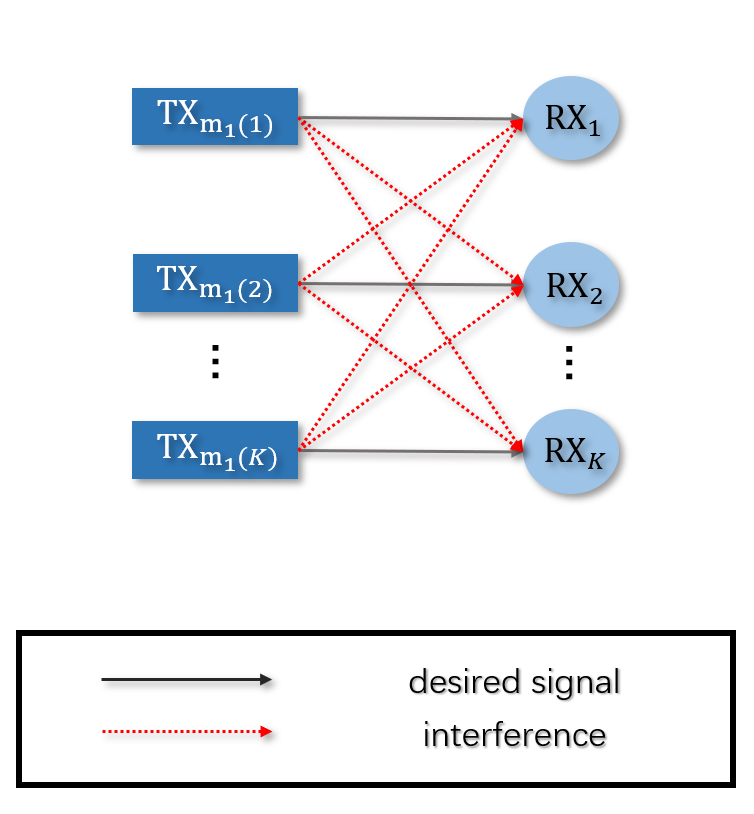
(a) Example 1: beamforming design for interference channels.

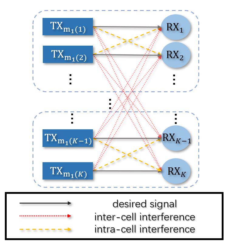
(b) Example 2: power allocation for interference broadcast channels.

(c) Example 3: cooperative beamforming design.

Fig. 1: Graph modeling for three typical examples.

As shown in Fig. 1LABEL:sub@fig-ex1, by modeling the BSs and UEs as TX-nodes and RX-nodes respectively, we can incorporate the maximum transmit power budget $\mathbf{p}=[P_{1},\cdots,P_{K}]^{T}$ and the noise standard deviation $\bm{\sigma}=[\sigma_{1},\cdots,\sigma_{K}]^{T}$ as the features on the TX-nodes and RX-nodes, respectively. Moreover, the feature vector on the $(m,k)$-th edge contains both the channel state information $\mathbf{h}_{m,k}$ and the indicator of direct communication or interference link:

$$\boldsymbol{H}_{(m,k,:)}=\begin{cases}[\mathbf{h}_{m,k}^{T},\mathbf{0}^{T}]^{T},\leavevmode\nobreak\ \text{if}\leavevmode\nobreak\ m=m_{1}(k),\cr[\mathbf{0}^{T},\mathbf{h}_{m,k}^{T}]^{T},\leavevmode\nobreak\ \text{otherwise},\end{cases}$$ (5)

where we adopt the idea of one-hot encoding to embed the information of direct communication or interference links. On the other hand, since $\mathbf{v}_{k}$ is the beamforming variable corresponding to the $(m_{1}(k),k,:)$-th TX-RX pair and $m_{1}(\cdot)$ is a one-to-one mapping, we can either define $\mathbf{v}_{k}$ on the $(m_{1}(k),k,:)$-th edge, the $k$-th RX-node, or the $m_{1}(k)$-th TX-node. Without loss of generality, we put $\mathbf{v}_{k}$ on the $(m_{1}(k),k,:)$-th fiber of the edge variable tensor $\boldsymbol{V}$, and problem (4) can be reformulated on the heterogeneous graph as

$$\mathop{\max}\limits_{\phi\left(\cdot,\cdot,\cdot\right)}\leavevmode\nobreak\ \sum^{K}_{k=1}\log_{2}\left(1+\text{SINR}_{k}\right),$$ (6a)

$$\leavevmode\nobreak\ \text{s.t.}\leavevmode\nobreak\ \leavevmode\nobreak\ \leavevmode\nobreak\ \leavevmode\nobreak\ \boldsymbol{V}=\phi\left(\mathbf{p},\bm{\sigma},\boldsymbol{H}\right),\leavevmode\nobreak\ \text{with}\leavevmode\nobreak\ \left\lVert\mathbf{v}_{k}\right\rVert^{2}\leq P_{m_{1}(k)},\leavevmode\nobreak\ \forall k\in\mathcal{K}.$$ (6b)

Comparing (6) with (1), the objective function (6a) is a specification of (1a). Particularly, the features $\mathbf{p}$, $\bm{\sigma}$, and $\boldsymbol{H}$ correspond to $\mathbf{F}_{\text{TX}}$, $\mathbf{F}_{\text{RX}}$, and $\boldsymbol{E}$, respectively, and the variable $\boldsymbol{V}$ corresponds to $\boldsymbol{\it{\Xi}}$.

Example 2: Power Allocation for Interference Broadcast Channels. Consider a $B$-cell downlink cellular network, where each BS serves $Q$ UEs. Each BS is equipped with $N$ antennas and each UE is equipped with a single antenna. The normalized beamforming vector of UE $q\in\mathcal{Q}\triangleq\left\{1,\cdots,Q\right\}$ in cell $b\in\mathcal{B}\triangleq\left\{1,\cdots,B\right\}$ is denoted as $\mathbf{w}_{q_{b}}\in\mathbb{C}^{N}$, while the channel between BS $b^{\prime}$ and UE $q$ in cell $b$ is denoted as $\mathbf{h}_{b^{\prime},q_{b}}\in\mathbb{C}^{N}$. Then the received signal at UE $q$ in cell $b$ is given by

$$y_{q_{b}}=\sqrt{p_{q_{b}}}\mathbf{h}_{b,q_{b}}^{H}\mathbf{w}_{q_{b}}s_{q_{b}} +\sum^{Q}_{q^{\prime}=1,q^{\prime}\neq q}\sqrt{p_{q^{\prime}_{b}}}\mathbf{h}_{b,q_{b}}^{H}\mathbf{w}_{q^{\prime}_{b}}s_{q^{\prime}_{b}}$$ (7)

$$+\sum^{B}_{b^{\prime}=1,b^{\prime}\neq b}\sum^{Q}_{q^{\prime}=1}\sqrt{p_{q^{\prime}_{b^{\prime}}}}\mathbf{h}_{b^{\prime},q_{b}}^{H}\mathbf{w}_{q^{\prime}_{b^{\prime}}}s_{q^{\prime}_{b^{\prime}}}+n_{q_{b}},\leavevmode\nobreak\ \forall q\in\mathcal{Q},\forall b\in\mathcal{B},$$

where $s_{q_{b}}$ and $p_{q_{b}}$ are the desired symbol and transmit power, respectively, the second term is the intra-cell interference, the third term is the inter-cell interference, and $n_{q_{b}}\sim\mathcal{C}\mathcal{N}(0,\sigma_{q_{b}}^{2})$ is the additive complex Gaussian noise. Correspondingly, the SINR is given by

$$\text{SINR}_{q_{b}}=\frac{\left|\mathbf{h}_{b,q_{b}}^{H}\mathbf{w}_{q_{b}}\right|^{2}p_{q_{b}}}{\sum^{Q}_{q^{\prime}=1,q^{\prime}\neq q}\left|\mathbf{h}_{b,q_{b}}^{H}\mathbf{w}_{q^{\prime}_{b}}\right|^{2}p_{q^{\prime}_{b}}+\sum^{B}_{b^{\prime}=1,b^{\prime}\neq b}\sum^{Q}_{q^{\prime}=1}\left|\mathbf{h}_{b^{\prime},q_{b}}^{H}\mathbf{w}_{q^{\prime}_{b^{\prime}}}\right|^{2}p_{q^{\prime}_{b^{\prime}}}+\sigma_{q_{b}}^{2}},\leavevmode\nobreak\ \forall q\in\mathcal{Q},\forall b\in\mathcal{B}.$$ (8)

The power allocation problem for sum rate maximization can be formulated as:

$$\mathop{\max}\limits_{\left\{p_{q_{b}}\right\}_{q\in\mathcal{Q},b\in\mathcal{B}}}\leavevmode\nobreak\ \sum^{B}_{b=1}\sum^{Q}_{q=1}\log_{2}\left(1+\text{SINR}_{q_{b}}\right),$$ (9a)

$$\leavevmode\nobreak\ \leavevmode\nobreak\ \leavevmode\nobreak\ \leavevmode\nobreak\ \leavevmode\nobreak\ \text{s.t.}\leavevmode\nobreak\ \leavevmode\nobreak\ \leavevmode\nobreak\ \leavevmode\nobreak\ \leavevmode\nobreak\ \leavevmode\nobreak\ 0\leq\sum^{Q}_{q=1}p_{q_{b}}\leq P_{b},\leavevmode\nobreak\ \forall b\in\mathcal{B},$$ (9b)

where $P_{b}$ is the maximum transmit power budget of BS $b$.

As observed in (8), the inner product of $\mathbf{h}_{b,q_{b}}$ and $\mathbf{w}_{q_{b}}$ has $BQ\times BQ$ combinations, leading to $K=BQ$ equivalent TX-nodes and $K$ RX-nodes, respectively. By modeling each BS as $Q$ TX-nodes, and each UE as an RX-node, we define two one-to-one mappings $\psi_{\text{TX}}(\cdot,\cdot)$ and $\psi_{\text{RX}}(\cdot,\cdot)$ from $\mathcal{B}\times\mathcal{Q}$ to $\mathcal{M}$ and $\mathcal{K}$, respectively. Let $k=\psi_{\text{RX}}(b,q)$, and then for RX_k, the TX-nodes can be divided into three types as shown in Fig. 1LABEL:sub@fig-ex2. The first type is the TX-node that serves RX_k, denoted as TX${}_{m_{1}(k)}$, where $m_{1}(k)\triangleq\psi_{\text{TX}}(b,q)$. The second type consists of other TX-nodes in the same cell as RX_k, denoted as TX${}_{m_{2}(k)}$, where $m_{2}(k)\in\mathcal{M}_{2}(k)\triangleq\left\{\psi_{\text{TX}}(b,q^{\prime})|\forall q^{\prime}\in\mathcal{Q},q^{\prime}\neq q\right\}$. The third type consists of TX-nodes in other cells, denoted as TX${}_{m_{3}(k)}$, where $m_{3}(k)\in\mathcal{M}_{3}(k)\triangleq\left\{\psi_{\text{TX}}(b^{\prime},q^{\prime})|\forall b^{\prime}\in\mathcal{B},b^{\prime}\neq b,\forall q^{\prime}\in\mathcal{Q}\right\}$. Accordingly, the equivalent channel gain between different TX-nodes and RX_k can be written as three types:

$$g_{m_{1}(k),k} \triangleq\left|\mathbf{h}_{b,q_{b}}^{H}\mathbf{w}_{q_{b}}\right|,$$ (10a)

$$g_{m_{2}(k),k} \triangleq\left|\mathbf{h}_{b,q_{b}}^{H}\mathbf{w}_{q^{\prime}_{b}}\right|,\leavevmode\nobreak\ \forall q^{\prime}\in\mathcal{Q},q^{\prime}\neq q,$$ (10b)

$$g_{m_{3}(k),k} \triangleq\left|\mathbf{h}_{b^{\prime},q_{b}}^{H}\mathbf{w}_{q^{\prime}_{b^{\prime}}}\right|,\leavevmode\nobreak\ \forall b^{\prime}\in\mathcal{B},b^{\prime}\neq b,\forall q^{\prime}\in\mathcal{Q}.$$ (10c)

We incorporate the maximum transmit power budget $\mathbf{p}=\left[\tilde{P}_{1},\cdots,\tilde{P}_{K}\right]^{T}$ and the noise standard deviation $\bm{\sigma}=[\sigma_{1},\cdots,\sigma_{K}]^{T}$ as the features on the TX-nodes and RX-nodes, respectively, where $\tilde{P}_{m_{1}(k)}=P_{b}$. Moreover, the feature vector on the $(m,k)$-th edge contains both the equivalent channel gain $g_{m,k}$ and the indicator of direct communication, intra-cell interference, or inter-cell interference link:

$$\boldsymbol{G}_{(m,k,:)} = \begin{cases}[g_{m,k},0,0]^{T},\leavevmode\nobreak\ &\text{if}\leavevmode\nobreak\ m=m_{1}(k),\cr[0,g_{m,k},0]^{T},\leavevmode\nobreak\ &\text{if}\leavevmode\nobreak\ m=m_{2}(k),\cr[0,0,g_{m,k}]^{T},\leavevmode\nobreak\ &\text{otherwise},\cr\end{cases}$$ (11)

where we adopt the idea of one-hot encoding to embed the information of direct communication, inter-cell interference, or intra-cell interference links. On the other hand, since $p_{q_{b}}$ is the power allocation variable corresponding to the $(m_{1}(k),k,:)$-th TX-RX pair and $m_{1}(\cdot)$ is a one-to-one mapping, we can either define $p_{q_{b}}$ on the $(m_{1}(k),k,:)$-th edge, the $k$-th RX-node, or the $m_{1}(k)$-th TX-node. Without loss of generality, putting the unknown power allocation variable $p_{q_{b}}$ on the $(m_{1}(k),k,:)$-th fiber of the edge variable tensor $\boldsymbol{P}$, problem (9) can be reformulated on the heterogeneous graph as

$$\mathop{\max}\limits_{\phi\left(\cdot,\cdot,\cdot\right)}\leavevmode\nobreak\ \sum_{b=1}^{B}\sum_{q=1}^{Q}\log_{2}\left(1+\text{SINR}_{q_{b}}\right),$$ (12a)

$$\leavevmode\nobreak\ \text{s.t.}\leavevmode\nobreak\ \leavevmode\nobreak\ \leavevmode\nobreak\ \boldsymbol{P}=\phi\left(\mathbf{p},\bm{\sigma},\boldsymbol{G}\right),\leavevmode\nobreak\ \text{with}\leavevmode\nobreak\ 0\leq\sum^{Q}_{q=1}p_{q_{b}}\leq P_{b},\leavevmode\nobreak\ \forall b\in\mathcal{B}.$$ (12b)

Comparing (12) with (1), the objective function (12a) is a specification of (1a). In particular, the features $\mathbf{p}$, $\bm{\sigma}$, and $\boldsymbol{G}$ correspond to $\mathbf{F}_{\text{TX}}$, $\mathbf{F}_{\text{RX}}$, and $\boldsymbol{E}$, respectively, and the variable $\boldsymbol{P}$ corresponds to $\boldsymbol{\it{\Xi}}$.

Example 3: Cooperative Beamforming Design. Consider a downlink system where $M$ BSs serve $K$ UEs cooperatively. Each BS is equipped with $N$ antennas and serves all UEs, while each UE is equipped with a single antenna and served by all BSs. The channel between the $m$-th BS and the $k$-th UE can be defined as $\mathbf{h}_{m,k}\in\mathbb{C}^{N}$. The beamforming vector used by the $m$-th BS for serving the $k$-th UE is denoted as $\mathbf{v}_{m,k}\in\mathbb{C}^{N}$. With $s_{k}$ denoting the desired symbol of the $k$-th UE, the received signal at the $k$-th UE is expressed as

$$y_{k}=\sum^{M}_{m=1}\mathbf{h}^{H}_{m,k}\mathbf{v}_{m,k}s_{k}+\sum^{K}_{k^{\prime}=1,k^{\prime}\neq k}\sum^{M}_{m=1}\mathbf{h}^{H}_{m,k}\mathbf{v}_{m,k^{\prime}}s_{k^{\prime}}+n_{k},\leavevmode\nobreak\ \forall k\in\mathcal{K},$$ (13)

where $n_{k}\sim\mathcal{CN}(0,\sigma_{k}^{2})$ is the additive complex Gaussian noise. The SINR can be written as

$$\text{SINR}_{k}=\frac{\left|\sum^{M}_{m=1}\mathbf{h}^{H}_{m,k}\mathbf{v}_{m,k}\right|^{2}}{\sum^{K}_{k^{\prime}=1,k^{\prime}\neq k}\left|\sum^{M}_{m=1}\mathbf{h}^{H}_{m,k}\mathbf{v}_{m,k^{\prime}}\right|^{2}+\sigma^{2}_{k}},\leavevmode\nobreak\ \forall k\in\mathcal{K}.$$ (14)

The cooperative beamforming design problem for sum rate maximization can be formulated as

$$\mathop{\max}\limits_{\left\{\mathbf{v}_{m,k}\right\}_{m\in\mathcal{M},k\in\mathcal{K}}}\leavevmode\nobreak\ \sum^{K}_{k=1}\log_{2}\left(1+\text{SINR}_{k}\right),$$ (15a)

$$\leavevmode\nobreak\ \leavevmode\nobreak\ \leavevmode\nobreak\ \leavevmode\nobreak\ \leavevmode\nobreak\ \leavevmode\nobreak\ \leavevmode\nobreak\ \text{s.t.}\leavevmode\nobreak\ \leavevmode\nobreak\ \leavevmode\nobreak\ \leavevmode\nobreak\ \leavevmode\nobreak\ \leavevmode\nobreak\ \leavevmode\nobreak\ \sum^{K}_{k=1}\left\lVert\mathbf{v}_{m,k}\right\rVert^{2}\leq P_{m},\leavevmode\nobreak\ \forall m\in\mathcal{M},$$ (15b)

where $P_{m}$ denotes the maximum power budget of BS $m$.

As illustrated in Fig. 1LABEL:sub@fig-ex3, by modeling the BSs and UEs as TX-nodes and RX-nodes respectively, we can incorporate the maximum transmit power budget $\mathbf{p}=[P_{1},\cdots,P_{M}]^{T}$ and the noise standard deviation $\bm{\sigma}=[\sigma_{1},\cdots,\sigma_{K}]^{T}$ as the features on the TX-nodes and RX-nodes, respectively. Moreover, the feature vector on the $(m,k)$-th edge can be defined as $\boldsymbol{H}_{(m,k,:)}=\mathbf{h}_{m,k}$. Unlike the previous examples, the unknown beamforming variable $\mathbf{v}_{m,k}$ is not a variable corresponding to a TX/RX-node, but rather corresponding to the $(m,k)$-th TX-RX pair. Thus, $\mathbf{v}_{m,k}$ can only be defined on the $(m,k)$-th edge. Putting $\mathbf{v}_{m,k}$ on the $(m,k,:)$-th fiber of the edge variable tensor $\boldsymbol{V}$, problem (15) can be reformulated on the heterogeneous graph as

$$\mathop{\max}\limits_{\phi\left(\cdot,\cdot,\cdot\right)}\leavevmode\nobreak\ \sum^{K}_{k=1}\log_{2}\left(1+\text{SINR}_{k}\right),$$ (16a)

$$\leavevmode\nobreak\ \text{s.t.}\leavevmode\nobreak\ \leavevmode\nobreak\ \leavevmode\nobreak\ \boldsymbol{V}=\phi\left(\mathbf{p},\bm{\sigma},\boldsymbol{H}\right),\leavevmode\nobreak\ \text{with}\leavevmode\nobreak\ \sum^{K}_{k=1}\left\lVert\mathbf{v}_{m,k}\right\rVert^{2}\leq P_{m},\leavevmode\nobreak\ \forall m\in\mathcal{M}.$$ (16b)

Comparing (16) with (1), the objective function (16a) is a specification of (1a). Particularly, the features $\mathbf{p}$, $\bm{\sigma}$, and $\boldsymbol{H}$ correspond to $\mathbf{F}_{\text{TX}}$, $\mathbf{F}_{\text{RX}}$, and $\boldsymbol{E}$, respectively, and the variable $\boldsymbol{V}$ corresponds to $\boldsymbol{\it{\Xi}}$.

Notice that in the cooperative beamforming application, beamforming variables exist on the communication links between TX-nodes and RX-nodes and should therefore be defined on the edges. However, existing GNNs [17] [30] are only equipped with the node-update mechanism, which cannot cope with the more complicated problem of cooperative beamforming design, where each TX-node serves multiple RX-nodes and each RX-node is also served by multiple TX-nodes.

II-C PE Property

A unique property of beamforming design and power allocation is that the optimized strategy is independent of the indices of TX-nodes and RX-nodes. In particular, the learned mapping function $\phi(\cdot,\cdot,\cdot)$ is inherently permutation equivariant with respect to TX-nodes and RX-nodes, i.e., if the indices of any two TX-nodes or RX-nodes are exchanged, $\phi(\cdot,\cdot,\cdot)$ should output a corresponding permutation.

To visualize this, we show a heterogeneous graph before and after permutations of TX-nodes and RX-nodes in Fig. 2. Define two permutations $\pi_{\text{TX}}(\cdot)$ and $\pi_{\text{RX}}(\cdot)$, and let ${\text{TX}}_{m}$ and ${\text{RX}}_{k}$ in Fig. 2LABEL:sub@fig-case1 be re-ordered as $\dot{\text{TX}}_{\pi_{\text{TX}}(m)}$ and $\dot{\text{RX}}_{\pi_{\text{RX}}(k)}$ in Fig. 2LABEL:sub@fig-case2, where $\pi_{\text{TX}}(1)=2$, $\pi_{\text{TX}}(2)=1$, $\pi_{\text{RX}}(1)=3$, $\pi_{\text{RX}}(2)=1$, and $\pi_{\text{RX}}(3)=2$. Accordingly, the graph features satisfy

$$\mathbf{\dot{f}}_{\text{TX},\pi_{\text{TX}}(m)} =\mathbf{{f}}_{\text{TX},m},\leavevmode\nobreak\ \forall m\in\mathcal{M},$$ (17a)

$$\mathbf{\dot{f}}_{\text{RX},\pi_{\text{RX}}(k)} =\mathbf{{f}}_{\text{RX},k},\leavevmode\nobreak\ \forall k\in\mathcal{K},$$ (17b)

$$\boldsymbol{\it{\dot{E}}}_{(\pi_{\text{TX}}(m),\pi_{\text{RX}}(k),:)} =\boldsymbol{\it{{E}}}_{(m,k,:)},\leavevmode\nobreak\ \forall(m,k)\in\mathcal{E}.$$ (17c)

Let $\left(\mathbf{\dot{S}}_{\text{TX}},\mathbf{\dot{S}}_{\text{RX}},\boldsymbol{\it{\dot{\Xi}}}\right)=\phi\left(\mathbf{\dot{F}}_{\text{TX}},\mathbf{\dot{F}}_{\text{RX}},\boldsymbol{\it{\dot{E}}}\right)$ and $\left(\mathbf{{S}}_{\text{TX}},\mathbf{{S}}_{\text{RX}},\boldsymbol{\it{{\Xi}}}\right)=\phi\left(\mathbf{{F}}_{\text{TX}},\mathbf{{F}}_{\text{RX}},\boldsymbol{\it{{E}}}\right)$ be the corresponding outputs of the mapping function $\phi(\cdot,\cdot,\cdot)$, respectively. Since $\left(\mathbf{\dot{F}}_{\text{TX}},\mathbf{\dot{F}}_{\text{RX}},\boldsymbol{\it{\dot{E}}}\right)$ is just a re-ordering of the TX-nodes and RX-nodes in $\left(\mathbf{{F}}_{\text{TX}},\mathbf{{F}}_{\text{RX}},\boldsymbol{\it{{E}}}\right)$, the corresponding outputs of the mapping function $\phi(\cdot,\cdot,\cdot)$ should satisfy

$$\mathbf{\dot{s}}_{\text{TX},\pi_{\text{TX}}(m)} =\mathbf{{s}}_{\text{TX},m},\leavevmode\nobreak\ \forall m\in\mathcal{M},$$ (18a)

$$\mathbf{\dot{s}}_{\text{RX},\pi_{\text{RX}}(k)} =\mathbf{{s}}_{\text{RX},k},\leavevmode\nobreak\ \forall k\in\mathcal{K},$$ (18b)

$$\boldsymbol{\it{\dot{\Xi}}}_{(\pi_{\text{TX}}(m),\pi_{\text{RX}}(k),:)} =\boldsymbol{\it{{\Xi}}}_{(m,k,:)},\leavevmode\nobreak\ \forall(m,k)\in\mathcal{E}.$$ (18c)

We will show in the next section that (18) can be guaranteed by the proposed ENGNN with properly designed edge/node-update mechanisms.

(a) Original heterogeneous graph.

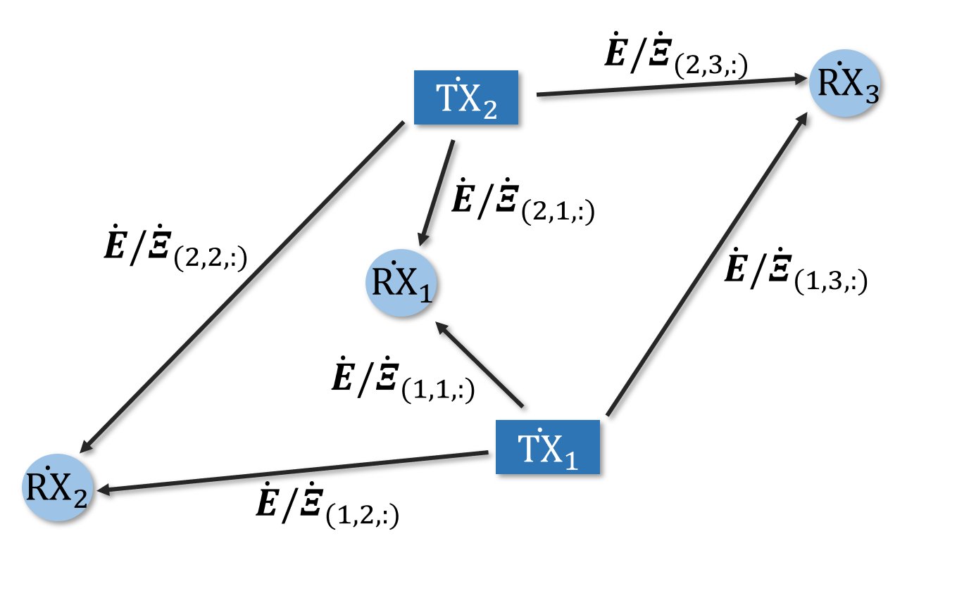
(b) Heterogeneous graph after permutations of TX-nodes and RX-nodes.

Fig. 2: Permutation equivariance illustration.

III The Proposed ENGNN

In this section, we propose a customized neural network architecture to represent the mapping function $\phi(\cdot,\cdot,\cdot)$ from $\left(\mathbf{F}_{\text{TX}},\mathbf{F}_{\text{RX}},\boldsymbol{E}\right)$ to $\left(\mathbf{S}_{\text{TX}},\mathbf{S}_{\text{RX}},\boldsymbol{\it{\Xi}}\right)$ in problem (1). The proposed neural network architecture incorporates both an edge-update mechanism and a node-update mechanism into a GNN and hence we name it as ENGNN. We will show that the proposed ENGNN enjoys the PE property given by (18).

III-A Overall Architecture

The proposed ENGNN consists of a preprocessing layer, $L$ updating layers, and a postprocessing layer as illustrated in Fig. 3. The preprocessing layer transforms the input features $\left(\mathbf{F}_{\text{TX}},\mathbf{F}_{\text{RX}},\boldsymbol{E}\right)$ into the initial node- and edge-representations $\left(\mathbf{F}_{\text{TX}}^{(0)}\in\mathbb{R}^{M\times\breve{d}_{\text{TX}}},\mathbf{F}_{\text{RX}}^{(0)}\in\mathbb{R}^{K\times\breve{d}_{\text{RX}}},\boldsymbol{E}^{(0)}\in\mathbb{R}^{M\times K\times\breve{d}_{\text{E}}}\right)$, where $\breve{d}_{\text{TX}}$, $\breve{d}_{\text{RX}}$, and $\breve{d}_{\text{E}}$ denote the dimensions of the representations on TX-nodes, RX-nodes, and edges, respectively. These representations will be updated according to node- and edge-update mechanisms in the $L$ updating layers, where the $l$-th updating layer takes $\left(\mathbf{F}_{\text{TX}}^{(l-1)},\mathbf{F}_{\text{RX}}^{(l-1)},\boldsymbol{E}^{(l-1)}\right)$ as the inputs and then outputs the updated representations $\left(\mathbf{F}_{\text{TX}}^{(l)},\mathbf{F}_{\text{RX}}^{(l)},\boldsymbol{E}^{(l)}\right)$. The dimensions of the representations will not change in the updating layers. Finally, the postprocessing layer transforms the graph representations $\left(\mathbf{F}_{\text{TX}}^{(L)},\mathbf{F}_{\text{RX}}^{(L)},\boldsymbol{E}^{(L)}\right)$ into variables $\left(\mathbf{S}_{\text{TX}},\mathbf{S}_{\text{RX}},\boldsymbol{\it{\Xi}}\right)$.

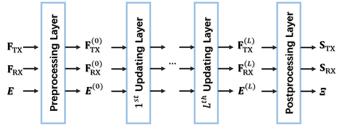
Fig. 3: The overall architecture of the proposed ENGNN, which contains a preprocessing layer, $L$ updating layers, and a postprocessing layer.

III-B Preprocessing Layer

The preprocessing layer converts complex-valued features (if any) on TX-nodes, RX-nodes, and edges into the real-valued form that can be processed by neural networks, and then transforms the real-valued features into initial representations. Specifically, the inputs of the preprocessing layer $\left(\mathbf{F}_{\text{TX}},\mathbf{F}_{\text{RX}},\boldsymbol{E}\right)$ are converted into their corresponding real-valued forms $\left(\hat{\mathbf{F}}_{\text{TX}},\hat{\mathbf{F}}_{\text{RX}},\hat{\boldsymbol{E}}\right)$, where the $m$-th row of $\mathbf{F}_{\text{TX}}$, the $k$-th row of $\mathbf{F}_{\text{RX}}$, and the $(m,k)$-th fiber of $\boldsymbol{E}$ are given by

$$\hat{\mathbf{f}}_{\text{TX},m} =\left[\Re\left\{\mathbf{f}_{\text{TX},m}\right\}^{T},\Im\left\{\mathbf{f}_{\text{TX},m}\right\}^{T}\right]^{T},\leavevmode\nobreak\ \forall m\in\mathcal{M},$$ (19a)

$$\hat{\mathbf{f}}_{\text{RX},k} =\left[\Re\left\{\mathbf{f}_{\text{RX},k}\right\}^{T},\Im\left\{\mathbf{f}_{\text{RX},k}\right\}^{T}\right]^{T},\leavevmode\nobreak\ \forall k\in\mathcal{K},$$ (19b)

$$\boldsymbol{\hat{E}}_{(m,k,:)} =\left[\Re\left\{\boldsymbol{E}_{(m,k,:)}\right\}^{T},\Im\left\{\boldsymbol{E}_{(m,k,:)}\right\}^{T}\right]^{T},\leavevmode\nobreak\ \forall(m,k)\in\mathcal{E}.$$ (19c)

Then, the initial representations of TX-nodes, RX-nodes, and edges are transformed by a one-layer MLP with rectified linear unit (ReLU) as the activation function:

$$\mathbf{f}_{\text{TX},m}^{(0)} =\text{ReLU}\left(\mathbf{W}_{\text{TX}}^{\text{pre}}\hat{\mathbf{f}}_{\text{TX},m}+\mathbf{b}_{\text{TX}}^{\text{pre}}\right),\leavevmode\nobreak\ \forall m\in\mathcal{M},$$ (20a)

$$\mathbf{f}_{\text{RX},k}^{(0)} =\text{ReLU}\left(\mathbf{W}_{\text{RX}}^{\text{pre}}\hat{\mathbf{f}}_{\text{RX},k}+\mathbf{b}_{\text{RX}}^{\text{pre}}\right),\leavevmode\nobreak\ \forall k\in\mathcal{K},$$ (20b)

$$\boldsymbol{E}^{(0)}_{(m,k,:)} =\text{ReLU}\left(\mathbf{\mathbf{W}^{\text{pre}}\boldsymbol{\hat{E}}}_{(m,k,:)}+\mathbf{b}^{\text{pre}}\right),\leavevmode\nobreak\ \forall(m,k)\in\mathcal{E},$$ (20c)

where $\mathbf{W}_{\text{TX}}^{\text{pre}}\in\mathbb{R}^{\breve{d}_{\text{TX}}\times 2d_{\text{TX}}}$, $\mathbf{b}_{\text{TX}}^{\text{pre}}\in\mathbb{R}^{\breve{d}_{\text{TX}}}$, $\mathbf{W}_{\text{RX}}^{\text{pre}}\in\mathbb{R}^{\breve{d}_{\text{RX}}\times 2d_{\text{RX}}}$, $\mathbf{b}_{\text{RX}}^{\text{pre}}\in\mathbb{R}^{\breve{d}_{\text{RX}}}$, $\mathbf{W}^{\text{pre}}\in\mathbb{R}^{\breve{d}_{\text{ E}}\times 2d_{\text{E}}}$, and $\mathbf{b}^{\text{pre}}\in\mathbb{R}^{\breve{d}_{\text{E}}}$ are trainable parameters.

III-C Updating Layer

The inputs and outputs of the updating layer $l\in\left\{1,\cdots,L\right\}$ are $\left(\mathbf{F}_{\text{TX}}^{(l-1)},\mathbf{F}_{\text{RX}}^{(l-1)},\boldsymbol{E}^{(l-1)}\right)$ and $\left(\mathbf{F}_{\text{TX}}^{(l)},\mathbf{F}_{\text{RX}}^{(l)},\boldsymbol{E}^{(l)}\right)$, respectively. We next show the node- and edge-update mechanisms in the $l$-th updating layer.

III-C1 Node-Update Mechanism

The update of node representations in the $l$-th updating layer takes $\left(\mathbf{F}_{\text{TX}}^{(l-1)},\mathbf{F}_{\text{RX}}^{(l-1)},\boldsymbol{E}^{(l-1)}\right)$ as the inputs, and then outputs the updated node representations $\left(\mathbf{F}_{\text{TX}}^{(l)},\mathbf{F}_{\text{RX}}^{(l)}\right)$. In particular, when updating the representation of TX_m, the inputs are composed of the previous layer’s representations of TX_m, the neighboring RX-nodes RX_k, and edges $(m,k)$ for all $k\in\mathcal{N}^{\text{TX}}_{m}$, where $\mathcal{N}^{\text{TX}}_{m}$ is the set of neighboring RX-nodes of TX_m. First, the input representations on RX_k and edge $(m,k)$ are concatenated and then processed by an MLP. Next, the processing results from all RX_k with $k\in\mathcal{N}^{\text{TX}}_{m}$ are combined by an aggregation function (e.g., mean or max aggregators), which extracts information from all the neighboring RX-nodes regardless of their input order. Finally, the input representation of TX_m and the aggregated result are concatenated and then processed by another MLP. The above procedure gives the following TX-update mechanism in the $l$-th updating layer:

$$\mathbf{f}_{\text{TX},m}^{(l)}=\text{MLP}_{2}^{(l)}\left(\mathbf{f}_{\text{TX},m}^{(l-1)},\text{AGG}_{\text{TX}}^{(l)}\left\{\text{MLP}_{1}^{(l)}\left(\mathbf{f}_{\text{RX},k}^{(l-1)},\boldsymbol{E}_{(m,k,:)}^{(l-1)}\right)\right\}_{k\in\mathcal{N}^{\text{TX}}_{m}}\right),\leavevmode\nobreak\ \forall m\in\mathcal{M},$$ (21)

where $\mathbf{f}_{\text{TX},m}^{(l-1)}$ is the $m$-th row of $\mathbf{F}_{\text{TX}}^{(l-1)}$, $\mathbf{f}_{\text{RX},k}^{(l-1)}$ is the $k$-th row of $\mathbf{F}_{\text{RX}}^{(l-1)}$, $\boldsymbol{E}_{(m,k,:)}^{(l-1)}$ is the $(m,k)$-th fiber of $\boldsymbol{E}^{(l-1)}$, $\text{MLP}_{1}^{(l)}$ and $\text{MLP}_{2}^{(l)}$ are two MLPs, and $\text{AGG}_{\text{TX}}^{(l)}$ is an aggregation function. Similarly, the RX-update mechanism in the $l$-th updating layer reverses the roles of TX-nodes and UE-nodes in (21):

$$\mathbf{f}_{\text{RX},k}^{(l)}=\text{MLP}_{4}^{(l)}\left(\mathbf{f}_{\text{RX},k}^{(l-1)},\text{AGG}_{\text{RX}}^{(l)}\left\{\text{MLP}_{3}^{(l)}\left(\mathbf{f}_{\text{TX},m}^{(l-1)},\boldsymbol{E}_{(m,k,:)}^{(l-1)}\right)\right\}_{m\in\mathcal{N}^{\text{RX}}_{k}}\right),\leavevmode\nobreak\ \forall k\in\mathcal{K},$$ (22)

where $\mathcal{N}^{\text{RX}}_{k}$ is the set of neighboring TX-nodes of RX_k, $\text{MLP}_{3}^{(l)}$ and $\text{MLP}_{4}^{(l)}$ are two MLPs, and $\text{AGG}_{\text{RX}}^{(l)}$ is an aggregation function.

Notice that the representations of TX-nodes and RX-nodes are updated differently in the proposed ENGNN. This is different from the previous work MPGNN [17] in which the node representations are updated homogeneously. Moreover, in the proposed ENGNN, the input edge representations $\boldsymbol{E}_{(m,k,:)}^{(l-1)}$ in (21) and (22) are with superscript $(l-1)$ and hence are also updated (see the edge-update mechanism). Taking a similar analysis in [17], we can show that (21) and (22) satisfy the following PE property:

Property 1 (PE in Node-Update Mechanism): The node-update mechanism (21) and (22) are permutation equivariant with respect to TX-nodes and RX-nodes, respectively. Specifically, for any permutations $\pi_{\text{TX}}(\cdot)$ and $\pi_{\text{RX}}(\cdot)$, we have

$$\mathbf{f}_{\text{TX},\pi_{\text{TX}}(m)}^{(l)} = \text{MLP}_{2}^{(l)}\left(\mathbf{f}_{\text{TX},\pi_{\text{TX}}(m)}^{(l-1)},\text{AGG}_{\text{TX}}^{(l)}\left\{\text{MLP}_{1}^{(l)}\left(\mathbf{f}_{\text{RX},k}^{(l-1)},\boldsymbol{E}_{\left(\pi_{\text{TX}}(m),k,:\right)}^{(l-1)}\right)\right\}_{k\in\mathcal{N}^{\text{TX}}_{\pi_{\text{TX}}(m)}}\right),\leavevmode\nobreak\ \forall m\in\mathcal{M},$$ (23a)

$$\mathbf{f}_{\text{RX},\pi_{\text{RX}}(k)}^{(l)} = \text{MLP}_{4}^{(l)}\left(\mathbf{f}_{\text{RX},\pi_{\text{RX}}(k)}^{(l-1)},\text{AGG}_{\text{RX}}^{(l)}\left\{\text{MLP}_{3}^{(l)}\left(\mathbf{f}_{\text{TX},m}^{(l-1)},\boldsymbol{E}_{\left(m,\pi_{\text{RX}}(k),:\right)}^{(l-1)}\right)\right\}_{m\in\mathcal{N}^{\text{RX}}_{\pi_{\text{RX}}(k)}}\right),\leavevmode\nobreak\ \forall k\in\mathcal{K}.$$ (23b)

III-C2 Edge-Update Mechanism

The update of edge representations in the $l$-th updating layer takes $\left(\mathbf{F}_{\text{TX}}^{(l-1)},\mathbf{F}_{\text{RX}}^{(l-1)},\boldsymbol{E}^{(l-1)}\right)$ as the inputs, and then outputs the updated edge representations $\boldsymbol{E}^{(l)}$. Different from the node-update mechanism, where the neighbors of a TX-node (or RX-node) are clearly defined as the connecting RX-nodes (or TX-nodes), it is more complicated to define the neighbors of an edge, let alone how to aggregate their representations. Notice that an edge may connect with other edges through either a TX-node or an RX-node. In particular, for the edge $(m,k)\in\mathcal{E}$, its neighboring edges through TX_m are $(m,k_{1}),\forall k_{1}\in\mathcal{N}^{\text{TX}}_{m}\setminus\{k\}$, while the neighboring edges through RX_k are $(m_{1},k),\forall m_{1}\in\mathcal{N}^{\text{RX}}_{k}\setminus\{m\}$. For example, in Fig. 4, the neighboring edges of edge $(1,1)$ through $\text{TX}_{1}$ are edge $(1,2)$ and edge $(1,3)$. On the other hand, the neighboring edge of edge $(1,1)$ through $\text{RX}_{1}$ is edge $(2,1)$. This causes the neighbors of an edge to be innately divided into two categories based on the connecting node. Consequently, different from the node-update mechanism (21) and (22), the edge-update mechanism should provide two different aggregations for the two types of neighboring edges.

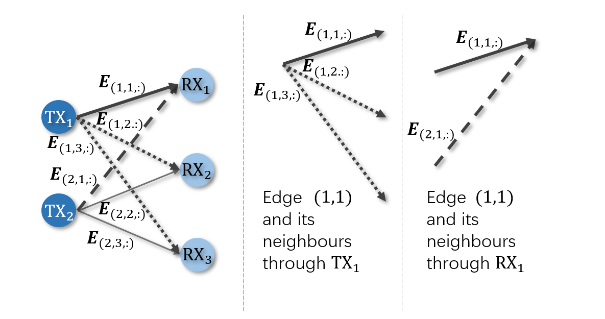
Fig. 4: The neighbors that share the connection with edge $(1,1)$ through $\text{TX}_{1}$ are edge $(1,2)$ and edge $(1,3)$, which are denoted by dotted lines. The neighbor that shares the connection with edge $(1,1)$ through $\text{RX}_{1}$ is edge $(2,1)$, which is denoted by a dashed line.

Specifically, when updating the representation of edge $(m,k)$, the inputs are composed of the previous representations of edge $(m,k)$, TX_m, RX_k, the neighboring edges $(m,k_{1}),\forall k_{1}\in\mathcal{N}^{\text{TX}}_{m}\setminus\{k\}$, and neighboring edges $(m_{1},k),\forall m_{1}\in\mathcal{N}^{\text{RX}}_{k}\setminus\{m\}$. The input representations of neighboring edges $(m,k_{1}),\forall k_{1}\in\mathcal{N}^{\text{TX}}_{m}\setminus\{k\}$ and the connecting node TX_m are concatenated and then processed by an MLP, while the input representations of neighboring edges $(m_{1},k),\forall m_{1}\in\mathcal{N}^{\text{RX}}_{k}\setminus\{m\}$ and the connecting node RX_k are concatenated and then processed by another MLP. The processing results of all the neighboring edges are aggregated and then concatenated with the input representation of edge $(m,k)$. An MLP is finally applied to produce the updated representation of edge $(m,k)$. We can express the above edge-update procedure in the $l$-th updating layer as

$$\boldsymbol{E}_{(m,k,:)}^{(l)}=\leavevmode\nobreak \text{MLP}_{7}^{(l)}\biggr{(}\boldsymbol{E}_{(m,k,:)}^{(l-1)},\text{AGG}_{\text{E}}^{(l)}\left\{\text{MLP}_{5}^{(l)}\left(\boldsymbol{E}_{(m,k_{1},:)}^{(l-1)},\mathbf{f}_{\text{TX},m}^{(l-1)}\right),\right.$$ (24)

$$\left.\text{MLP}_{6}^{(l)}\left(\boldsymbol{E}_{(m_{1},k,:)}^{(l-1)},\mathbf{f}_{\text{RX},k}^{(l-1)}\right)\right\}_{k_{1}\in\mathcal{N}^{\text{TX}}_{m}\setminus\{k\},m_{1}\in\mathcal{N}^{\text{RX}}_{k}\setminus\{m\}}\biggr{)},\leavevmode\nobreak\ \forall(m,k)\in\mathcal{E},$$

where $\boldsymbol{E}_{(m,k,:)}^{(l-1)}$ is the $(m,k)$-th fiber of $\boldsymbol{E}^{(l-1)}$, $\text{MLP}_{5}^{(l)}$, $\text{MLP}_{6}^{(l)}$, and $\text{MLP}_{7}^{(l)}$ are three MLPs, and $\text{AGG}_{\text{E}}^{(l)}$ is an aggregation function.

Compared with the node-update mechanism (21) and  (22), the edge-update mechanism (24) is more complicated, since the definition of neighbors in edge-update mechanism is more complex than that in the node-update one. In particular, the edge-update mechanism faces a more complicated situation where the neighboring edges are innately divided into two categories according to the two possible connected nodes. Consequently, different from the node-update mechanism (21) and (22), where the information from neighboring nodes are gathered by one MLP, the proposed edge-update mechanism applies two different transformations to extract the information from two different types of neighboring edges. We next show that (24) enjoys the following PE property:

Property 2 (PE in Edge-Update Mechanism): The edge-update mechanism (24) is permutation equivariant with respect to TX-nodes and RX-nodes. Specifically, for any permutations $\pi_{\text{TX}}(\cdot)$ and $\pi_{\text{RX}}(\cdot)$, we have

$$\boldsymbol{E}_{(\pi_{\text{TX}}(m),\pi_{\text{RX}}(k),:)}^{(l)}=\leavevmode\nobreak\ \text{MLP}_{7}^{(l)}\left(\boldsymbol{E}_{(\pi_{\text{TX}}(m),\pi_{\text{RX}}(k),:)}^{(l-1)},\text{AGG}_{\text{E}}^{(l)}\left\{\text{MLP}_{5}^{(l)}\left(\boldsymbol{E}_{(\pi_{\text{TX}}(m),k_{1},:)}^{(l-1)},\mathbf{f}_{\text{TX},\pi_{\text{TX}}(m)}^{(l-1)}\right),\right.\right.$$ (25)

$$\left.\left.\text{MLP}_{6}^{(l)}\left(\boldsymbol{E}_{(m_{1},\pi_{\text{RX}}(k),:)}^{(l-1)},\mathbf{f}_{\text{RX},\pi_{\text{RX}}(k)}^{(l-1)}\right)\right\}_{k_{1}\in\mathcal{N}^{\text{TX}}_{\pi_{\text{TX}}(m)}\setminus\left\{\pi_{\text{RX}}(k)\right\},m_{1}\in\mathcal{N}^{\text{RX}}_{\pi_{\text{RX}}(k)}\setminus\left\{\pi_{\text{TX}}(m)\right\}}\right),\leavevmode\nobreak\ \forall(m,k)\in\mathcal{E}.$$

Proof: See Appendix A.

III-D Postprocessing Layer

The postprocessing layer converts the graph representations $\left(\mathbf{F}_{\text{TX}}^{(L)},\mathbf{F}_{\text{RX}}^{(L)},\boldsymbol{E}^{(L)}\right)$ into the final output $\left(\mathbf{S}_{\text{TX}},\mathbf{S}_{\text{RX}},\boldsymbol{\it{\Xi}}\right)$. First, if the variables are complex, $\left(\mathbf{F}_{\text{TX}}^{(L)},\mathbf{F}_{\text{RX}}^{(L)},\boldsymbol{E}^{(L)}\right)$ are transformed into the complex form $\left(\mathbf{\tilde{S}}_{\text{TX}},\mathbf{\tilde{S}}_{\text{RX}},\boldsymbol{\it{\tilde{\Xi}}}\right)$ by

$$\left[\Re\left\{\mathbf{\tilde{s}}_{\text{TX},m}\right\}^{T},\Im\left\{\mathbf{\tilde{s}}_{\text{TX},m}\right\}^{T}\right]^{T} =\mathbf{W}_{\text{TX}}^{\text{post}}\mathbf{f}_{\text{TX},m}^{(L)}+\mathbf{b}_{\text{TX}}^{\text{post}},\leavevmode\nobreak\ \forall m\in\mathcal{M},$$ (26a)

$$\left[\Re\left\{\mathbf{\tilde{s}}_{\text{RX},k}\right\}^{T},\Im\left\{\mathbf{\tilde{s}}_{\text{RX},k}\right\}^{T}\right]^{T} =\mathbf{W}_{\text{RX}}^{\text{post}}\mathbf{f}_{\text{RX},k}^{(L)}+\mathbf{b}_{\text{RX}}^{\text{post}},\leavevmode\nobreak\ \forall k\in\mathcal{K},$$ (26b)

$$\left[\Re\left\{\boldsymbol{\it{\tilde{\Xi}}}_{(m,k,:)}\right\}^{T},\Im\left\{\boldsymbol{\it{\tilde{\Xi}}}_{(m,k,:)}\right\}^{T}\right]^{T} =\mathbf{W}^{\text{post}}\boldsymbol{E}_{(m,k.:)}^{(L)}+\mathbf{b}^{\text{post}},\leavevmode\nobreak\ \forall(m,k)\in\mathcal{E},$$ (26c)

where $\mathbf{W}_{\text{TX}}^{\text{post}}\in\mathbb{R}^{2d^{\prime}_{\text{TX}}\times\breve{d}_{\text{TX}}}$, $\mathbf{b}_{\text{TX}}^{\text{post}}\in\mathbb{R}^{2d^{\prime}_{\text{TX}}}$, $\mathbf{W}_{\text{RX}}^{\text{post}}\in\mathbb{R}^{2d^{\prime}_{\text{RX}}\times\breve{d}_{\text{RX}}}$, $\mathbf{b}_{\text{RX}}^{\text{post}}\in\mathbb{R}^{2d^{\prime}_{\text{RX}}}$, $\mathbf{W}^{\text{post}}\in\mathbb{R}^{2d^{\prime}_{\text{E}}\times\breve{d}_{\text{E}}}$, and $\mathbf{b}^{\text{post}}\in\mathbb{R}^{2d^{\prime}_{\text{E}}}$ are trainable parameters. Next, $\left(\mathbf{\tilde{S}}_{\text{TX}},\mathbf{\tilde{S}}_{\text{RX}},\boldsymbol{\it{\tilde{\Xi}}}\right)$ are normalized to satisfy the constraints (if any), obtaining the final output $\left(\mathbf{S}_{\text{TX}},\mathbf{S}_{\text{RX}},\boldsymbol{\it{\Xi}}\right)$.

III-E Key Insights

The proposed ENGNN for representing $\phi(\cdot,\cdot,\cdot)$ has been specified as a preprocessing layer, $L$ updating layers, and a postprocessing layer, where the preprocessing and postprocessing layers utilize edge/node-wise MLPs, and the $L$ updating layers are built on node- and edge-update mechanisms (21), (22), and (24). Next, we provide some key insights of the proposed ENGNN for learning the beamforming design and power allocation as follows.

III-E1 Permutation Equivariant with Respect to TX-nodes and RX-nodes

Proposition 1 (PE in ENGNN): The proposed ENGNN is permutation equivariant with respect to TX-nodes and RX-nodes. Specifically, for any permutations $\pi_{\text{TX}}(\cdot)$ and $\pi_{\text{RX}}(\cdot)$, denote a permuted problem instance of $\left(\mathbf{{F}}_{\text{TX}},\mathbf{{F}}_{\text{RX}},\boldsymbol{\it{{E}}}\right)$ as $\left(\mathbf{{\dot{F}}}_{\text{TX}},\mathbf{{\dot{F}}}_{\text{RX}},\boldsymbol{\it{{\dot{E}}}}\right)$, whose entries satisfy (17). The corresponding outputs of the proposed ENGNN, $\left(\mathbf{\dot{S}}_{\text{TX}},\mathbf{\dot{S}}_{\text{RX}},\boldsymbol{\it{\dot{\Xi}}}\right)=\phi\left(\mathbf{{\dot{F}}}_{\text{TX}},\mathbf{{\dot{F}}}_{\text{RX}},\boldsymbol{\it{{\dot{E}}}}\right)$ and $\left(\mathbf{S}_{\text{TX}},\mathbf{S}_{\text{RX}},\boldsymbol{\it{\Xi}}\right)=\phi\left(\mathbf{{F}}_{\text{TX}},\mathbf{{F}}_{\text{RX}},\boldsymbol{\it{{E}}}\right)$, always satisfy (18).

Proof: See Appendix B.

Proposition 1 implies that the proposed ENGNN is inherently incorporated with the PE property. This is in sharp contrast to the generic MLPs, which require all permutations of each training sample to approximate this property. Thus, the proposed ENGNN can reduce the sample complexity and training difficulty.

III-E2 Generalization on Different Numbers of TX-nodes and RX-nodes

In all the layers of the proposed ENGNN, the representations on different edges/TX-nodes/RX-nodes are transformed by the same architecture using the same trainable parameters. Therefore, the dimensions of the trainable parameters are independent of the numbers of TX-nodes and RX-nodes. This scale adaptability empowers ENGNN to be trained in a setup with a small graph size, while being deployed to a much larger wireless network for the inference.

III-E3 Tackling Edge Variables

The proposed ENGNN is equipped with an edge-update mechanism, which facilitates the update of the variables on graph edges. This allows ENGNN to be applied in a wider range of scenarios, where variables are defined between a pair of nodes.

IV Simulation Results

In this section, we demonstrate the superiority of the proposed ENGNN on the three examples introduced in Section II-B via simulations. We consider a downlink wireless network in a $2\times 2$ km² area, where the BSs and UEs are uniformly distributed. Each BS has a maximum transmit power of $33$ dBm. The path loss is $30.5+36.7\log_{10}d$ in dB, where $d$ is the distance in meters. The small scale channels follow Rayleigh fading and the noise power is $-99$ dBm.

For the proposed ENGNN, each aggregation function in (21), (22), and (24) is implemented by a max aggregator, which returns the element-wise maximum value of the inputs. All the MLPs in (21), (22), and (24) are implemented by $3$ linear layers, each followed by a ReLU activation function. In the training procedure, the number of epochs is set to $500$. Each epoch consists of $100$ mini-batches of training samples with a batch size of $256$. For each training sample, the BSs’ and UEs’ locations, and the small scale channels are randomly generated. A learning rate $\gamma=10^{-4}$ is adopted to update the trainable parameters of ENGNN by maximizing (1a) using RMSProp [35] in an unsupervised manner. After training, we test the average performance of $100$ samples. All the experiments are implemented using Pytorch on one NVIDIA V100 GPU ($32$ GB, SMX$2$).

IV-A Beamforming Design for Interference Channels

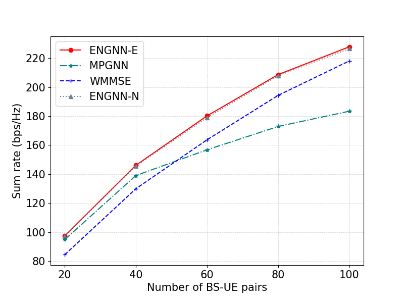
Fig. 5: Generalization on number of BS-UE pairs.

First, we demonstrate the performance of the proposed ENGNN on the problem of beamforming design for interference channels. During the training procedure, we set the wireless network with $20$ BS-UE pairs, where each BS is equipped with $2$ antennas. An ENGNN with $1$ updating layer is adopted, and the dimension of edge features $\breve{d}_{\text{E}}$ is set to $8$. As explained before (6), the beamforming variables in this scenario can be defined on either the edges or the nodes, which only affects the postprocessing layers. The corresponding simulation results are termed as ENGNN-E and ENGNN-N, respectively. For performance comparison, we include two state-of-the-art methods:

1. WMMSE: a widely used benchmark algorithm for sum rate maximization [8].

2. MPGNN: the latest learning based method for sum rate maximization in interference channels [17].

IV-A1 Generalization on Number of BS-UE Pairs

We first compare the performance of different approaches as the number of BS-UE pairs increases. In particular, ENGNN-E, ENGNN-N, MPGNN are trained on $20$ BS-UE pairs, while we test their performance in terms of sum rate on larger problem scales from $20$ to $100$ BS-UE pairs in Fig. 5. It can be seen that ENGNN-E, ENGNN-N, and MPGNN generalize well as the number of BS-UE pairs increases from $20$ to $40$. However, as the number of BS-UE pairs increases from $40$ to $100$, both ENGNN-E and ENGNN-N can still generalize very well, while the performance of MPGNN becomes worse than that of WMMSE. The superiority of ENGNN-E and ENGNN-N is owing to the proposed edge-update mechanism, which better extracts the features from channel states and hence further empowers the original node-update mechanism in MPGNN. Since ENGNN-E and ENGNN-N result in similar performance, we only show ENGNN-E in the rest of simulations and term it as ENGNN for simplicity.

IV-A2 Generalization on Noise Power

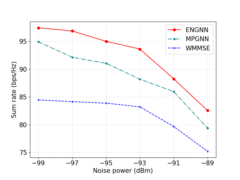
Fig. 6: Generalization on noise power.

To demonstrate the generalization performance on noise power, we set the noise power during the training procedure as $-99$ dBm, while we test the generalization performance under different noise powers from $-99$ dBm to $-89$ dBm. It can be seen from Fig. 6 that ENGNN consistently achieves higher sum rate than those of MPGNN and WMMSE, which demonstrates the superiority of ENGNN in generalizing to different noise powers.

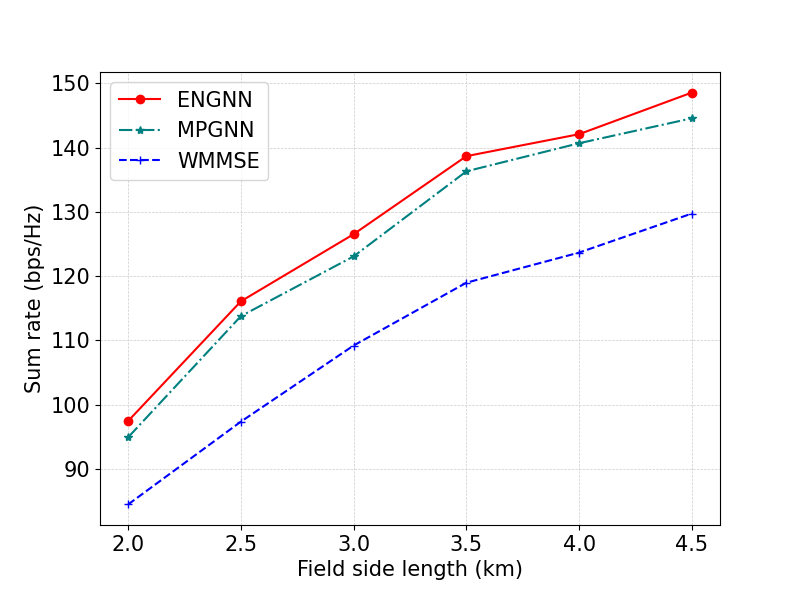
Fig. 7: Generalization on different levels of interference among BS-UE pairs.

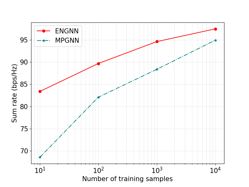
Fig. 8: Sample complexity comparison between ENGNN and MPGNN.

IV-A3 Generalization on Different Levels of Interference

In this experiment, we fix the field size during the training procedure as $2\times 2$ km², while we test the performance by varying the field size from $2\times 2$ km² to $4.5\times 4.5$ km². By keeping the distance between each BS and its serving UE within $50$-$250$ meters, the interference among different BS-UE pairs becomes weaker as the field size increases, and hence the sum rates of different approaches become higher in Fig. 7. Moreover, ENGNN consistently achieves higher sum rate than those of MPGNN and WMMSE as the field size increases, which demonstrates that ENGNN generalizes well on different levels of interference.

IV-A4 Sample Complexity Comparison

We further compare the performance of ENGNN and MPGNN when trained on different numbers of training samples in Fig. 8. It can be seen that ENGNN outperforms MPGNN especially when the number of training samples is small. In particular, when the number of training samples decreases to $10$-$100$, the sum rate of ENGNN only decreases to $83.39$-$89.68$ bps/Hz, while that of MPGNN decreases sharply to $68.60$-$82.10$ bps/Hz. The required number of training samples of ENGNN is less than $10\%$ of that of MPGNN when they achieve the same sum rate. This demonstrates the advantage of the proposed edge-update mechanism in sample complexity.

IV-B Power Allocation for Interference Broadcast Channels

Next, we demonstrate the performance of ENGNN on the problem of power allocation for interference broadcast channels. In the training procedure, we set the wireless network with $5$ BSs, with a minimum distance of $500$ meters between BSs. Each BS is equipped with $16$ antennas and serves $2$ UEs. We use zero-forcing beamforming to avoid multi-user interference. The ENGNN is set with $1$ updating layer and a dimension of $\breve{d}_{\text{E}}=32$ for the edge features. For performance comparison, we provide the simulation results of WMMSE and PGNN [30], which is the latest learning-based method for power allocation in interference broadcast channels.

IV-B1 Generalization on Number of UEs

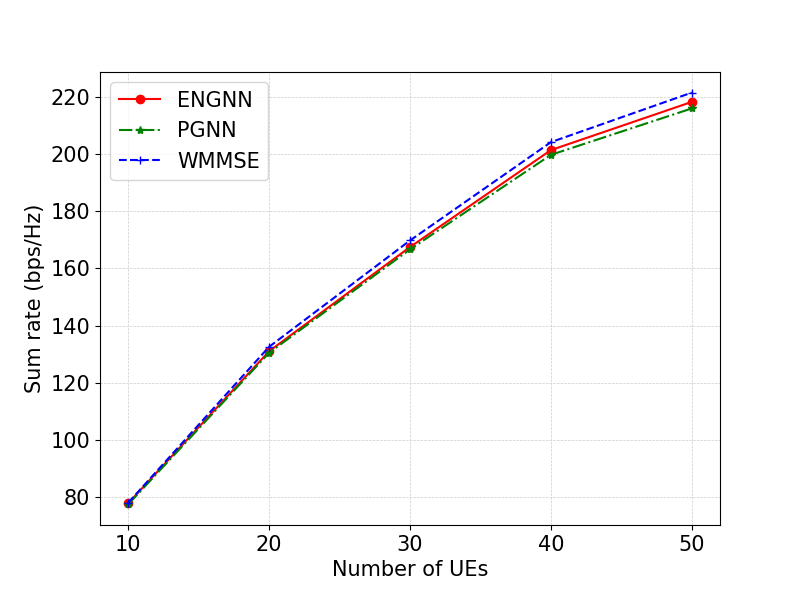
Fig. 9: Generalization on number of UEs for power allocation in interference broadcast channels.

We first compare the performance of different approaches as the number of UEs increases. In particular, both ENGNN and PGNN are trained under $10$ UEs, while we test their performance on larger problem scales from $10$ to $50$ UEs by varying the number of UEs in each cell from $2$ to $10$ in Fig. 9. It can be seen that both ENGNN and PGNN generalize well as the number of UEs increases from $10$ to $50$. However, ENGNN always outperforms PGNN, and achieves competitive performance compared to that of WMMSE under different numbers of UEs.

IV-B2 Generalization on Different Levels of Interference

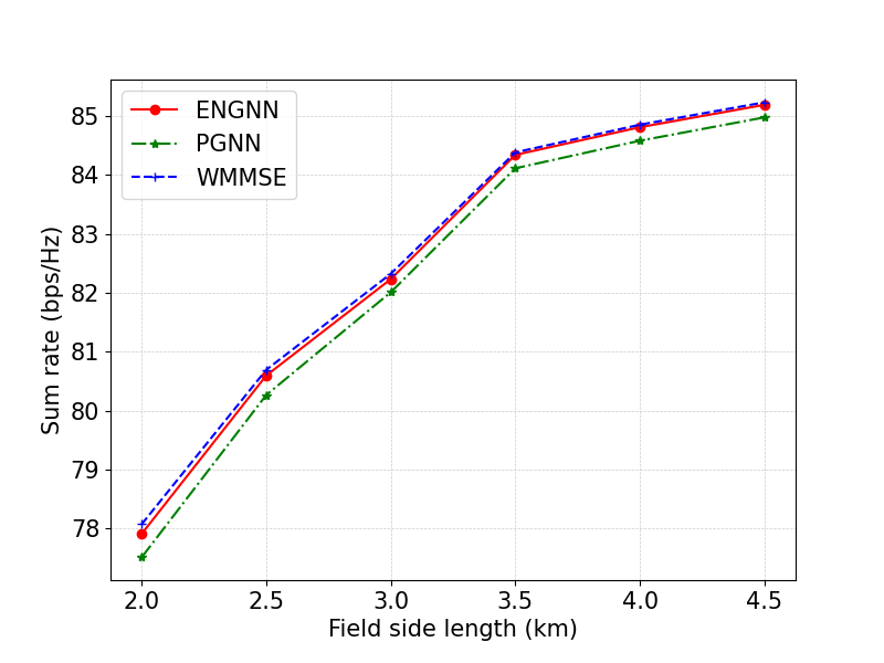
Fig. 10: Generalization on different levels of inter-cell interference.

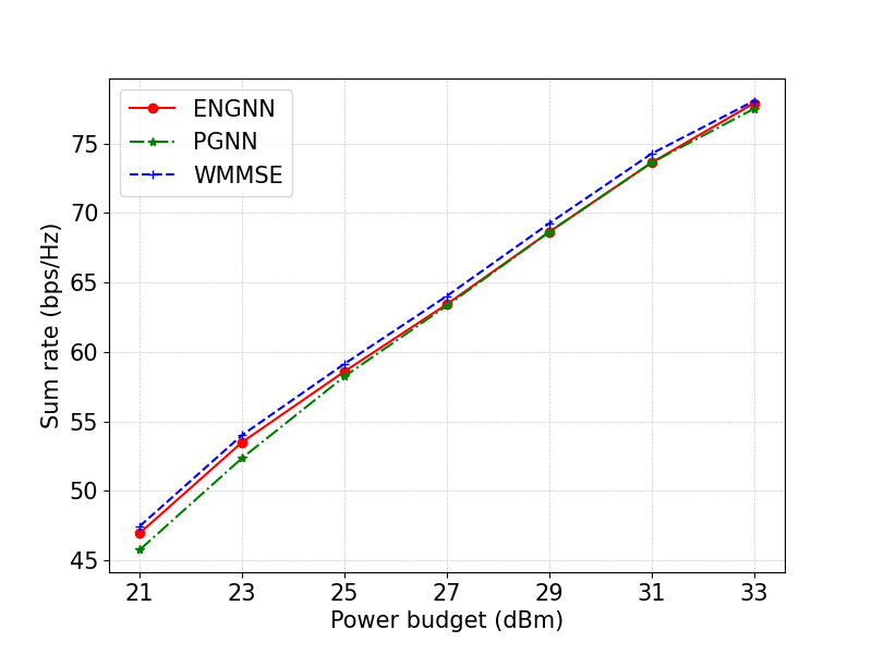
Fig. 11: Generalization on power budget.

To demonstrate the generalization ability on different levels of interference, during the training procedure, the field size is fixed as $2\times 2$ km², while we test the performance by varying the field size from $2\times 2$ km² to $4.5\times 4.5$ km². By keeping the distance between each BS and its serving UE within $50$-$250$ meters, the inter-cell interference becomes weaker as the field size increases, and hence the sum rate becomes higher in Fig. 10. It can be observed that the advantage of ENGNN over PGNN is stable as the field size increases, which demonstrates its superior generalization capability on different levels of interference.

IV-B3 Generalization on Power Budget

To demonstrate the generalization capability of ENGNN on different power budgets, we set the power budget at each BS as $33$ dBm during the training procedure, while we test the generalization performance under different power budgets from $21$ dBm to $33$ dBm in Fig. 11. It can be seen that both ENGNN and PGNN generalize well as the power budgets decreases from $33$ dBm to $21$ dBm. However, ENGNN always outperforms PGNN under different power budgets.

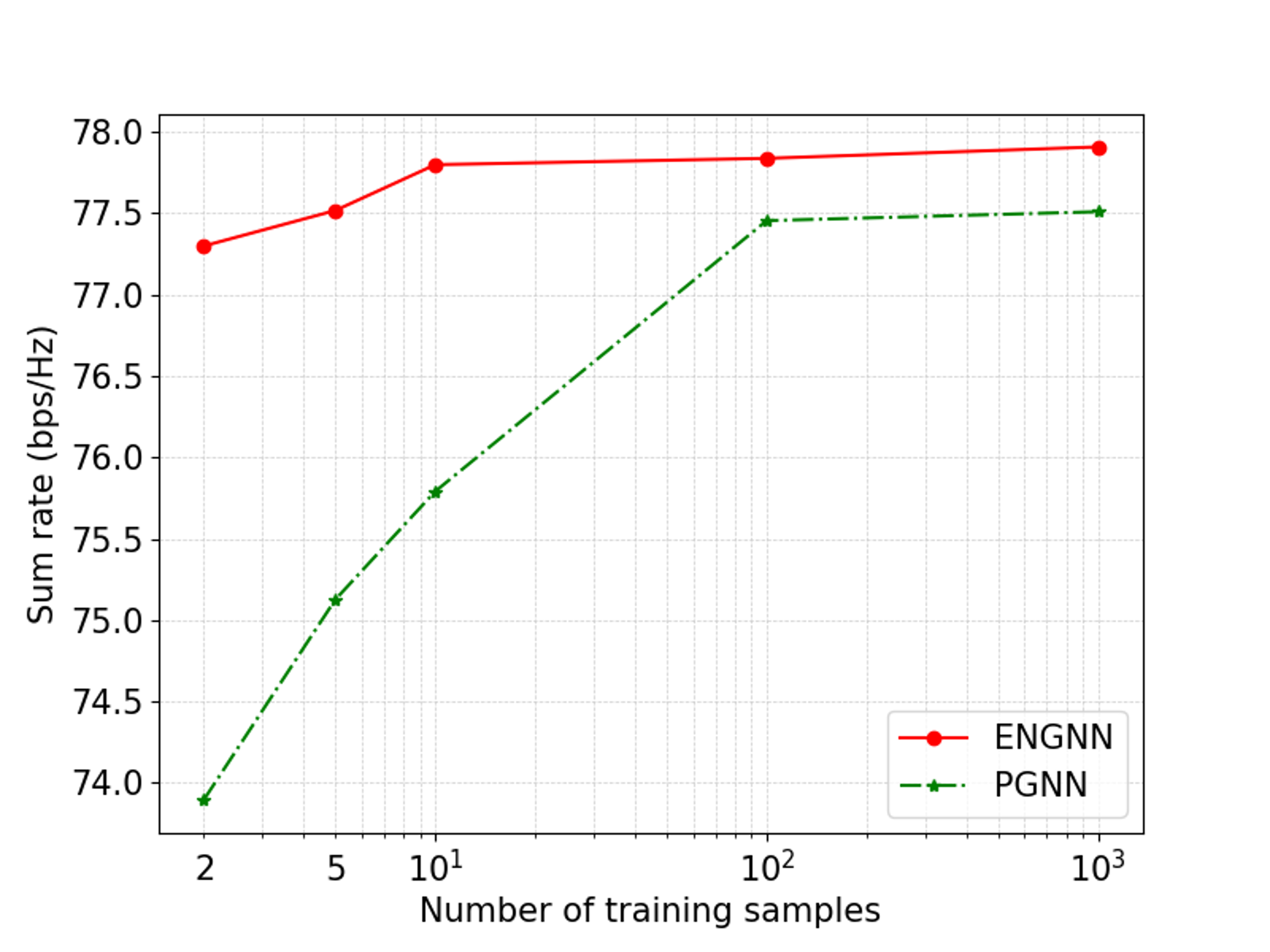
Fig. 12: Sample complexity comparison between ENGNN and PGNN.

IV-B4 Sample Complexity Comparison

We further compare the performance of ENGNN and PGNN when trained on different numbers of samples in Fig. 12. It can be seen that ENGNN outperforms PGNN especially when the number of training samples is small. Particularly, when the number of training samples decreases to $2$-$5$, the sum rate of ENGNN only drops to $77.30$-$77.52$ bps/Hz, while that of PGNN drops to $73.89$-$75.12$ bps/Hz. The required number of training samples of ENGNN is about $1\%$ of that of MPGNN when they achieve the same sum rate. This demonstrates the advantage of the proposed edge-update mechanism in sample complexity.

IV-C Cooperative Beamforming Design

Finally, we demonstrate the performance of ENGNN on the problem of cooperative beamforming design. During the training procedure, we set the wireless network with $5$ BSs and $2$ UEs. Each BS is equipped with $2$ antennas and the minimum distance between BSs is $500$ m. An ENGNN with $2$ updating layers is adopted, and the dimension of edge features $\breve{d}_{\text{E}}$ is set to $64$. For performance comparison, we include WMMSE and GP [7], the latter being a computationally efficient first-order algorithm for solving simply constrained optimization problems.

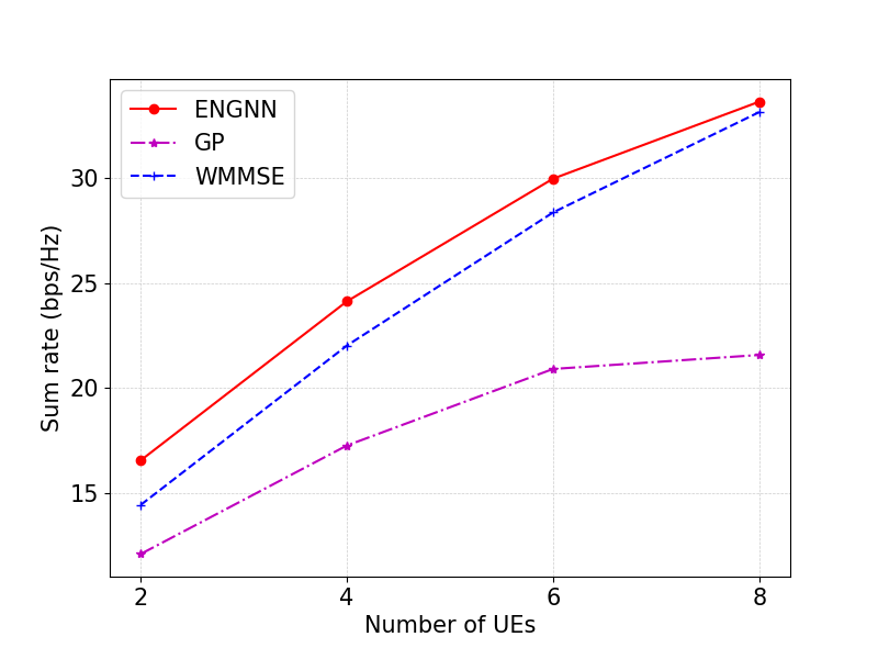
(a) Sum rate comparison

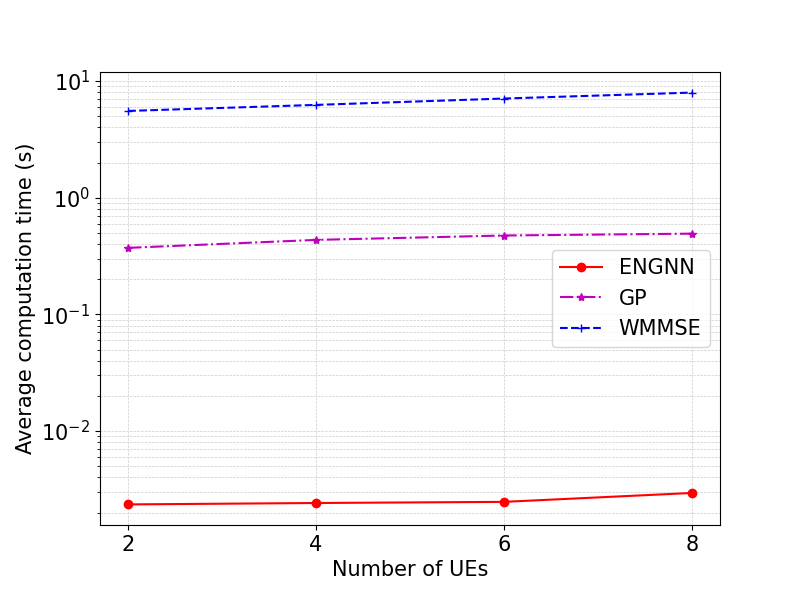
(b) Computation time comparison

Fig. 13: Generalization on number of UEs for cooperative beamforming.

IV-C1 Generalization on Number of UEs

To demonstrate the generalization ability of ENGNN with respect to different numbers of UEs, during the training procedure, the number of UEs is fixed as $2$, while we test the performance of the trained ENGNN by varying the number of UEs from $2$ to $8$. The performance comparison in terms of sum rate and computation time is shown in Fig. 13. We observe from Fig. 13LABEL:sub@fig-exp3_RX_sr that as the number of UEs increases, ENGNN always outperforms GP and WMMSE in terms of sum rate, which demonstrates its generalization ability with respect to different numbers of UEs. On the other hand, Fig. 13LABEL:sub@fig-exp3_RX_time shows that ENGNN achieves a remarkable running speed, with over $100$ times faster than that of GP and over $1000$ times faster than that of WMMSE due to the computationally efficient feed forward computations.

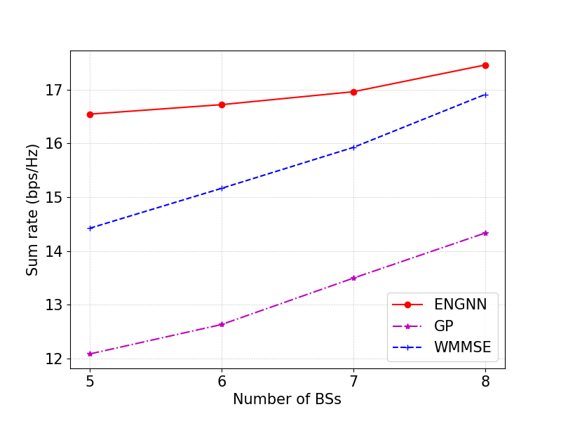
(a) Sum rate comparison

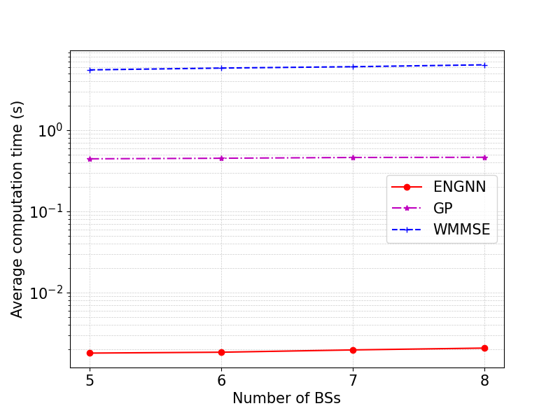
(b) Computation time comparison

Fig. 14: Generalization on numbers of BSs for cooperative beamforming.

IV-C2 Generalization on Number of BSs

We further demonstrate the generalization ability of ENGNN with respect to different numbers of BSs. Specifically, the number of BSs is fixed as $5$ during the training procedure, while we test the performance of the trained ENGNN by varying the number of BSs from $5$ to $8$. The performance comparison is shown in Fig. 14. We observe from Fig. 14LABEL:sub@fig-TX_sr that ENGNN achieves higher sum rate than those of GP and WMMSE under different numbers of BSs. Moreover, Fig. 14LABEL:sub@fig-TX_time shows that ENGNN achieves a much faster running speed than that of GP and WMMSE under different numbers of BSs.

V Conclusion

This paper proposed a general problem formulation on the heterogeneous graph for the radio resource management problems, where the unknown variables to be designed can be defined on both the graph nodes and edges. A novel edge-update mechanism with desired PE property was incorporated, and a general neural network architecture was designed based on it, which can represent the mapping function from the node/edge features to variables for the radio resource management problems. Simulation results demonstrated the superiority of the proposed architecture on three typical problems, with higher sum rate and much shorter computation time compared with state-of-the-art methods. Moreover, the proposed architecture generalizes well on different numbers of BSs and UEs, different noise variances, interference levels, and transmit power budgets.

Appendix A Proof of Property 2

Let $m^{\prime}=\pi_{\text{TX}}(m)$ and $k^{\prime}=\pi_{\text{RX}}(k)$. Substituting these two equations into (24), we have

$$\boldsymbol{E}_{(m^{\prime},k^{\prime},:)}^{(l)}=\leavevmode\nobreak \text{MLP}_{7}^{(l)}\left(\boldsymbol{E}_{(m^{\prime},k^{\prime},:)}^{(l-1)},\text{AGG}_{\text{E}}^{(l)}\left\{\text{MLP}_{5}^{(l)}\left(\boldsymbol{E}_{(m^{\prime},k^{\prime}_{1},:)}^{(l-1)},\mathbf{f}_{\text{TX},m^{\prime}}^{(l-1)}\right),\right.\right.$$ (27)

$$\left.\left.\text{MLP}_{6}^{(l)}\left(\boldsymbol{E}_{(m^{\prime}_{1},k^{\prime},:)}^{(l-1)},\mathbf{f}_{\text{RX},k^{\prime}}^{(l-1)}\right)\right\}_{k^{\prime}_{1}\in\mathcal{N}^{\text{TX}}_{m^{\prime}}\setminus\{k^{\prime}\},m^{\prime}_{1}\in\mathcal{N}^{\text{RX}}_{k^{\prime}}\setminus\{m^{\prime}\}}\right),\leavevmode\nobreak\ \forall(m^{\prime},k^{\prime})\in\mathcal{E},$$

which implies that for any $\pi_{\text{TX}}(\cdot)$ and $\pi_{\text{RX}}(\cdot)$, we always have (25).

Appendix B Proof of Proposition 1

Substituting (17) into (19) and (20) we have

$$\mathbf{\dot{f}}_{\text{TX},\pi_{\text{TX}}(m)}^{(0)} =\mathbf{f}_{\text{TX},m}^{(0)},\leavevmode\nobreak\ \forall m\in\mathcal{M},$$ (28a)

$$\mathbf{\dot{f}}_{\text{RX},\pi_{\text{RX}}(k)}^{(0)} =\mathbf{f}_{\text{RX},k}^{(0)},\leavevmode\nobreak\ \forall k\in\mathcal{K},$$ (28b)

$$\boldsymbol{\dot{E}}^{(0)}_{(\pi_{\text{TX}}(m),\pi_{\text{RX}}(k),:)} =\boldsymbol{E}^{(0)}_{(m,k,:)},\leavevmode\nobreak\ \forall(m,k)\in\mathcal{E}.$$ (28c)

Next, we substitute (28) into (21), (22), and (24). According to Property 1 and Property 2, we have

$$\mathbf{\dot{f}}_{\text{TX},\pi_{\text{TX}}(m)}^{(l)} =\mathbf{f}_{\text{TX},m}^{(l)},\leavevmode\nobreak\ \forall m\in\mathcal{M},\forall l=1,\cdots,L,$$ (29a)

$$\mathbf{\dot{f}}_{\text{RX},\pi_{\text{RX}}(k)}^{(l)} =\mathbf{f}_{\text{RX},k}^{(l)},\leavevmode\nobreak\ \forall k\in\mathcal{K},\forall l=1,\cdots,L,$$ (29b)

$$\boldsymbol{\dot{E}}^{(l)}_{(\pi_{\text{TX}}(m),\pi_{\text{RX}}(k),:)} =\boldsymbol{E}_{(m,k.:)}^{(L)},\leavevmode\nobreak\ \forall(m,k)\in\mathcal{E},\forall l=1,\cdots,L.$$ (29c)

Substituting (29) into (26), we obtain

$$\mathbf{\dot{\tilde{s}}}_{\text{TX},\pi_{\text{TX}}(m)} =\mathbf{\tilde{s}}_{\text{TX},m},\leavevmode\nobreak\ \forall m\in\mathcal{M},$$ (30a)

$$\mathbf{\dot{\tilde{s}}}_{\text{RX},\pi_{\text{RX}}(k)} =\mathbf{\tilde{s}}_{\text{RX},k},\leavevmode\nobreak\ \forall k\in\mathcal{K},$$ (30b)

$$\boldsymbol{\it{\dot{\tilde{\Xi}}}}_{(\pi_{\text{TX}}(m),\pi_{\text{RX}}(k),:)} =\boldsymbol{\it{\tilde{\Xi}}}_{(m,k,:)},\leavevmode\nobreak\ \forall(m,k)\in\mathcal{E}.$$ (30c)

Finally, since the normalization of $\left(\mathbf{\tilde{S}}_{\text{TX}},\mathbf{\tilde{S}}_{\text{RX}},\boldsymbol{\it{\tilde{\Xi}}}\right)$ is an edge/node-wise computation, the final outputs satisfy $\mathbf{\dot{s}}_{\text{TX},\pi_{\text{TX}}(m)}=\mathbf{{s}}_{\text{TX},m},\leavevmode\nobreak\ \forall m\in\mathcal{M}$, $\mathbf{\dot{s}}_{\text{RX},\pi_{\text{RX}}(k)}=\mathbf{{s}}_{\text{RX},k},\leavevmode\nobreak\ \forall k\in\mathcal{K}$, and $\boldsymbol{\it{\dot{\Xi}}}_{(\pi_{\text{TX}}(m),\pi_{\text{RX}}(k),:)}=\boldsymbol{\it{\Xi}}_{(m,k,:)},\leavevmode\nobreak\ \forall(m,k)\in\mathcal{E}$.

References

- [1] H. Zhang and H. Dai, “Cochannel interference mitigation and cooperative processing in downlink multicell multiuser MIMO networks,” EURASIP Journal on Wireless Communications and Networking, vol. 2004, no. 2, pp. 1–14, 2004.
- [2] Y. Shi, J. Zhang, K. B. Letaief, B. Bai, and W. Chen, “Large-scale convex optimization for ultra-dense Cloud-RAN,” IEEE Wireless Commun. Mag., vol. 22, no. 3, pp. 84–91, 2015.
- [3] Y. Li, M. Xia, and Y.-C. Wu, “First-order algorithm for content-centric sparse multicast beamforming in large-scale C-RAN,” IEEE Trans. Wireless Commun., vol. 17, no. 9, pp. 5959–5974, 2018.
- [4] H. He, X. Yu, J. Zhang, S. Song, and K. B. Letaief, “Cell-free massive MIMO for 6G wireless communication networks,” Journal of Communications and Information Networks, vol. 6, no. 4, pp. 321–335, 2021.
- [5] Y. Li, M. Xia, and Y.-C. Wu, “Energy-efficient precoding for non-orthogonal multicast and unicast transmission via first-order algorithm,” IEEE Trans. Wireless Commun., vol. 18, no. 9, pp. 4590–4604, 2019.
- [6] S. Mohammadi, M. Dong, and S. ShahbazPanahi, “Fast algorithm for joint unicast and multicast beamforming for large-scale massive MIMO,” IEEE Trans. Signal Process., vol. 70, pp. 5413–5428, 2022.
- [7] D. P. Bertsekas, “Nonlinear programming,” Journal of the Operational Research Society, vol. 48, no. 3, pp. 334–334, 1997.
- [8] Q. Shi, M. Razaviyayn, Z.-Q. Luo, and C. He, “An iteratively weighted MMSE approach to distributed sum-utility maximization for a MIMO interfering broadcast channel,” IEEE Trans. Signal Process., vol. 59, no. 9, pp. 4331–4340, 2011.
- [9] H. Sun, X. Chen, Q. Shi, M. Hong, X. Fu, and N. D. Sidiropoulos, “Learning to optimize: Training deep neural networks for interference management,” IEEE Trans. Signal Process., vol. 66, no. 20, pp. 5438–5453, 2018.
- [10] F. Liang, C. Shen, W. Yu, and F. Wu, “Towards optimal power control via ensembling deep neural networks,” IEEE Trans. Commun., vol. 68, no. 3, pp. 1760–1776, 2019.
- [11] W. Lee, M. Kim, and D.-H. Cho, “Deep power control: Transmit power control scheme based on convolutional neural network,” IEEE Commun. Lett., vol. 22, no. 6, pp. 1276–1279, 2018.
- [12] W. Xia, G. Zheng, Y. Zhu, J. Zhang, J. Wang, and A. P. Petropulu, “A deep learning framework for optimization of MISO downlink beamforming,” IEEE Trans. Commun., vol. 68, no. 3, pp. 1866–1880, 2019.
- [13] W. Cui, K. Shen, and W. Yu, “Spatial deep learning for wireless scheduling,” IEEE J. Sel. Areas Commun., vol. 37, no. 6, pp. 1248–1261, 2019.
- [14] Y. Shen, Y. Shi, J. Zhang, and K. B. Letaief, “LORM: Learning to optimize for resource management in wireless networks with few training samples,” IEEE Trans. Wireless Commun., vol. 19, no. 1, pp. 665–679, 2019.
- [15] M. Zhu, T.-H. Chang, and M. Hong, “Learning to beamform in heterogeneous massive MIMO networks,” arXiv preprint arXiv:2011.03971, 2020.
- [16] Y. Ma, Y. Shen, X. Yu, J. Zhang, S. H. Song, and K. B. Letaief, “Neural calibration for scalable beamforming in FDD massive MIMO with implicit channel estimation,” IEEE Trans. Wireless Commun., vol. 21, no. 11, pp. 9947–9961, 2022.
- [17] Y. Shen, Y. Shi, J. Zhang, and K. B. Letaief, “Graph neural networks for scalable radio resource management: Architecture design and theoretical analysis,” IEEE J. Sel. Areas Commun., vol. 39, no. 1, pp. 101–115, 2020.
- [18] M. Eisen and A. Ribeiro, “Optimal wireless resource allocation with random edge graph neural networks,” IEEE Trans. Signal Process., vol. 68, pp. 2977–2991, 2020.
- [19] Y. Shen, J. Zhang, and K. B. Letaief, “How neural architectures affect deep learning for communication networks?” in IEEE International Conference on Communications (ICC), 2022.
- [20] Y. Shen, J. Zhang, S. Song, and K. B. Letaief, “AI empowered resource management for future wireless networks,” in IEEE International Mediterranean Conference on Communications and Networking (MeditCom), 2021.
- [21] Y. Li, Z. Chen, Y. Wang, C. Yang, B. Ai, and Y.-C. Wu, “Heterogeneous transformer: A scale adaptable neural network architecture for device activity detection,” IEEE Trans. Wireless Commun., 2022, doi:10.1109/TWC.2022.3218579.
- [22] Y. Li, Z. Chen, G. Liu, Y.-C. Wu, and K.-K. Wong, “Learning to construct nested polar codes: An attention-based set-to-element model,” IEEE Commun. Lett., vol. 25, no. 12, pp. 3898–3902, 2021.
- [23] Y. Shen, J. Zhang, S. Song, and K. B. Letaief, “Graph neural networks for wireless communications: From theory to practice,” IEEE Trans. Wireless Commun., 2022, doi:10.1109/TWC.2022.3219840.
- [24] Z. Zhang, M. Tao, and Y.-F. Liu, “Learning to beamform in multi-group multicast with imperfect CSI,” in IEEE International Conference on Wireless Communications and Signal Processing (WCSP), 2022.
- [25] M. Lee, G. Yu, and G. Y. Li, “Graph embedding-based wireless link scheduling with few training samples,” IEEE Trans. Wireless Commun., vol. 20, no. 4, pp. 2282–2294, 2020.
- [26] A. Chowdhury, G. Verma, C. Rao, A. Swami, and S. Segarra, “Unfolding WMMSE using graph neural networks for efficient power allocation,” IEEE Trans. Wireless Commun., vol. 20, no. 9, pp. 6004–6017, 2021.
- [27] I. Nikoloska and O. Simeone, “Modular meta-learning for power control via random edge graph neural networks,” IEEE Trans. Wireless Commun., 2022, doi:10.1109/TWC.2022.3195352.
- [28] S. He, S. Xiong, W. Zhang, Y. Yang, J. Ren, and Y. Huang, “GBLinks: GNN-based beam selection and link activation for ultra-dense D2D mmWave networks,” IEEE Trans. Commun., vol. 25, no. 12, pp. 3898–3902, 2022.
- [29] C. Zhang, D. Song, C. Huang, A. Swami, and N. V. Chawla, “Heterogeneous graph neural network,” in ACM SIGKDD international conference on knowledge discovery & data mining, 2019.
- [30] J. Guo and C. Yang, “Learning power allocation for multi-cell-multi-user systems with heterogeneous graph neural network,” IEEE Trans. Wireless Commun., vol. 21, no. 2, pp. 884–897, 2021.
- [31] X. Zhang, H. Zhao, J. Xiong, X. Liu, L. Zhou, and J. Wei, “Scalable power control/beamforming in heterogeneous wireless networks with graph neural networks,” in IEEE Global Communications Conference (GLOBECOM), 2021.
- [32] J. Kim, H. Lee, S.-E. Hong, and S.-H. Park, “A bipartite graph neural network approach for scalable beamforming optimization,” IEEE Trans. Wireless Commun., 2022, doi:10.1109/TWC.2022.3193138.
- [33] T. Jiang, H. V. Cheng, and W. Yu, “Learning to reflect and to beamform for intelligent reflecting surface with implicit channel estimation,” IEEE J. Sel. Areas Commun., vol. 39, no. 7, pp. 1931–1945, 2021.
- [34] X. Zhang, H. Zhao, J. Wei, C. Yan, J. Xiong, and X. Liu, “Cooperative trajectory design of multiple UAV base stations with heterogeneous graph neural networks,” IEEE Trans. Wireless Commun., 2022, doi:10.1109/TWC.2022.3204794.
- [35] T. Tieleman, G. Hinton et al., “Lecture 6.5-RMSProp: Divide the gradient by a running average of its recent magnitude,” COURSERA: Neural networks for machine learning, vol. 4, no. 2, pp. 26–31, 2012.