0.1 Overview of the course

The goal of this course is to introduce algorithmic techniques for dealing with massive data: data so large that it does not fit in the computer’s memory. In this course, massive data will be abstracted by two main combinatorial objects: sets and sequences. Solutions dealing with massive data can be divided into two broad categories, covered in the two modules of the course: (lossless) compressed data structures and (lossy) data sketches.

Module 1 - Compressed data structures

In this module we will discuss material from Gonzalo Navarro’s book [24]. A compressed data structure supports fast queries on the data and uses a space proportional to the compressed data. This solution is typically lossless: the representation allows to fully reconstruct the original data. Here we exploit the fact that, in some applications, data is extremely redundant and can be considerably reduced in size (even by orders of magnitude) without losing any information by exploiting this redundancy. Interestingly it turns out that, usually, computation on compressed data can be performed faster than on the original (uncompressed) data: the field of compressed data structures exploits the natural duality between compression and computation to achieve this goal. The main results we will discuss in the course, compressed dictionaries and compressed text indexes, find important applications in information retrieval. They allow to pre-process a large collection of documents into a compressed data structure that allows locating substrings very quickly, without decompressing the data. These techniques today stand at the core of modern search engines and sequence-mapping algorithms in computational biology. Importantly, lossless techniques cannot break the information-theoretic lower bound for representing data. For example, since the number of subsets of cardinality $m$ of $\{1,\dots,n\}$ is $\binom{n}{m}$, the information-theoretic lower bound for storing such a subset is $\log_{2}\binom{n}{m}=m\log(n/m)+O(m)$ bits. No lossless data structure can use asymptotically less space than this bound for all such subsets.

Module 2 - Data sketches

In the second module, covered in these notes, we will resort to lossy compression and throw away some features of the data in order to reduce its size, usually breaking the information-theoretic lower bound.

In Chapter 2 we show that any set of cardinality $m$ can be stored with a filter data structure in just $O(m)$ bits, provided that we accept a small probability that membership queries fail.

In Chapters 3 and 4 we see how to shrink even more the size of our data while still being able to compute useful information on it. The most important concept here is sketching. Using clever randomized algorithms, we show how to reduce large data sets to sub-linear representations: for example, a set of cardinality $m$ over universe of cardinality $n$ can be stored in just $O(\mathrm{polylog}(m)+\mathrm{polylog}(n))$ bits using a data sketch supporting useful queries such as set similarity and cardinality estimation (approximately and with a bounded probability of error). Sketches can be computed off-line in order to reduce the dataset’s size and/or speed up the computation of distances (Chapter 3), or on-line on data streams (Chapter 4), where data is thrown away as soon as it arrives (only data sketches are kept).

Material

The proofs of these notes have been put together from various sources whose links can be found in the bibliography. The lectures follow also material from Leskovec et al.’s book [21] (Mining of massive data sets), Amit Chakrabarti’s notes on data stream algorithms [5], Gonzalo Navarro’s book [24] (compressed data structures), and Demetrescu and Finocchi’s chapter on algorithms for data streams from the book [30].

Chapter 1 Basics

1.1 Random variables

A random variable (R.V.) $X$ is a variable that takes values from some sample space $\Omega$ according to the outcomes of a random phenomenon. $\Omega$ is also called the support of $X$. Said otherwise, $X$ takes values in $\Omega$ according to some probability distribution. A random variable can be discrete if $|\Omega|$ is countable (examples: coin tosses or integer numbers), or continuous (for example, if it takes any real value in some interval). When considering multiple R.V.s with supports $\Omega_{1},\dots,\Omega_{n}$, the sample space is the Cartesian product of the individual sample spaces: $\Omega=\Omega_{1}\times\dots\times\Omega_{n}$. In these notes the support of a R.V. will either be a set of integers or an interval of real numbers.

1.1.1 Distribution function

We indicate with $F(x)=P(X\leq x)$ the cumulative distribution function of X: the probability that $X$ takes a value in $\Omega$ smaller than or equal to $x$. $P(X=x)=f(x)$ is the probability mass function (for discrete R.V.s) or the probability density function (for continuous R.V.s). For discrete R.V.s, this is the probability that $X$ takes value $x$. For continuous R.V.s, it’s the function satisfying $F(x)=\int_{-\infty}^{x}f(x)\,dx$.

Example 1.1.1.

Take the example of fair coin tosses. Then, $X\in\{0,1\}$ (0=tail, 1=head) is a discrete random variable with probability mass function $P(X=0)=P(X=1)=0.5$.

1.1.2 Events

An event is a subset of the sample space, i.e. a set of assignments for all the R.V.s under consideration. Each event has a probability to happen. For example, $A=\{0\leq X\leq 1\}$ is the event indicating that $X$ takes a value between $0$ and $1$. $P(A\cup B)$ is the probability that either $A$ or $B$ happens. $P(A\cap B)$ is the probability that both $A$ and $B$ happen. Sometimes we will also use the symbols $\vee$ and $\wedge$ in place of $\cup$ and $\cap$ (with the same meaning). $P(A|B)$ indicates the probability that $A$ happens, provided that $B$ has already happened. In general, we have:

$$P(A\cap B)=P(A)\cdot P(B|A)$$

We say that two events $A$ and $B$ are independent if $P(A\cap B)=P(A)\cdot P(B)$ or, equivalently, that $P(A|B)=P(A)$ and $P(B|A)=P(B)$: the probability that both happen simultaneously is the product of the probabilities that they happen individually. Said otherwise, the fact that one of the two events has happened, does not influence the happening of the other event.

Example 1.1.2.

Consider throwing two fair coins, and indicate $A=\{first\ coin=head\}$ and $B=\{second\ coin=head\}$. The two events are clearly independent, so

$$P(A\cap B)=P(A)\cdot P(B)=0.5\cdot 0.5=0.25$$

On the other hand, consider throwing a coin in front of a mirror, and the two events $A=\{coin=head\}$ and $B=\{coin\ in\ the\ mirror=head\}$. We still have $P(A)=P(B)=0.5$ (the events, considered separately, have both probability $0.5$ to happen), but the two events are clearly dependent! In fact, $P(B|A)=1\neq P(B)=0.5$. So: $P(A\cap B)=P(A)\cdot P(B|A)=P(A)\cdot 1=0.5$.

We can generalize pairwise-independence to a sequence of R.V.s:

Definition 1.1.3 ($k$-wise independence).

Let $W=\{X_{1},\dots,X_{n}\}$ be a set of $n$ random variables. We say that this set is $k$-wise independent, for $k\leq n$, iff $P(\bigwedge_{j=1}^{k}X_{i_{j}}=x_{i_{j}})=\prod_{j=1}^{k}P(X_{i_{j}}=x_{i_{j}})$ for any subset $\{X_{i_{1}},\dots,X_{i_{k}}\}\subseteq W$ of $k$ random variables. For $k=n$, we also say that the random variables are fully independent.

We will often deal with dependent random variables. A useful bound that we will use is the following:

Lemma 1.1.4 (Union bound).

For any set of (possibly dependent) events $\{A_{1},A_{2},\dots,A_{n}\}$ we have that:

$$P(\cup_{i=1}^{n}A_{i})\leq\sum_{i=1}^{n}P(A_{i})$$

The union bound can sometimes give quite uninformative results since the right hand-side sum can exceed 1. The bound becomes extremely useful, however, when dealing with rare events: in this case, the probability on the right hand-side could be much smaller than 1. This will be indeed the case in some of our applications.

We finally mention the law of total probability:

Lemma 1.1.5 (Law of total probability).

If $B_{i}$ for $i=1,\dots,k$ is a partition of the sample space, then for any event $A$:

$$P(A)=\sum_{i=1}^{k}P(A\cap B_{i})=\sum_{i=1}^{k}P(B_{i})P(A|B_{i})$$

1.1.3 Expected value and variance

Intuitively, the expected value (or mean) $E[X]$ of a numeric random variable $X$ is the arithmetic mean of a large number of independent realizations of $X$. Formally, it is defined as $E[X]=\sum_{x\in\Omega}x\cdot f(x)$ for discrete R.V.s and $E[X]=\int_{-\infty}^{+\infty}x\cdot f(x)\,dx$ for continuous R.V.s.

Some useful properties of the expected value that we will use:

Lemma 1.1.6 (Linearity of expectation).

Let $a_{i}$ be constants and $X_{i}$ be (any) random variables, for $i=1,\dots,n$. Then $E[\sum_{i=1}^{n}a_{i}X_{i}]=\sum_{i=1}^{n}a_{i}E[X_{i}]$

Proof.

For simplicity we consider the cases of $E[X+Y]$ and $E[aX]$. The claim follows easily. $E[X+Y]$ is computed using the law of total probability:

$$\begin{array}[]{rcl}E[X+Y]&=&\sum_{i,j}(x_{i}+y_{j})P(X=x_{i}\wedge Y=y_{j})\\ &=&\sum_{i,j}x_{i}\cdot P(X=x_{i}\wedge Y=y_{j})+\sum_{i,j}y_{j}\cdot P(X=x_{i}\wedge Y=y_{j})\\ &=&\sum_{i}x_{i}\sum_{j}P(X=x_{i}\wedge Y=y_{j})+\sum_{j}y_{j}\sum_{i}P(X=x_{i}\wedge Y=y_{j})\\ &=&\sum_{i}x_{i}\cdot P(X=x_{i})+\sum_{j}y_{j}\cdot P(Y=y_{j})\\ &=&E[X]+E[Y]\end{array}$$

and $E[aX]=\sum_{i}a\cdot x_{i}\cdot P(X=x_{i})=a\sum_{i}x_{i}\cdot P(X=x_{i})=a\cdot E[X]$. ∎

Also, the expected value of a constant $a$ is the constant itself: $E[a]=a$ (a constant $a$ can be regarded as a random variable that takes value $a$ with probability 1).

In general $E[X\cdot Y]\neq E[X]\cdot E[Y]$. Equality holds if $X$ and $Y$ are independent, though:

$$\begin{array}[]{rcl}E[XY]&=&\sum_{i,j}x_{i}y_{j}P(X=x_{i}\wedge Y=y_{j})\\ &=&\sum_{i,j}x_{i}y_{j}P(X=x_{i})P(Y=y_{j})\\ &=&\Big{(}\sum_{i}x_{i}P(X=x_{i})\Big{)}\cdot\left(\sum_{j}y_{j}P(Y=y_{j})\right)\\ &=&E[X]E[Y]\end{array}$$

More in general (prove it as an exercise):

Lemma 1.1.7.

If $X_{1},\dots,X_{n}$ are fully independent, then $E[\prod_{i=1}^{n}X_{i}]=\prod_{i=1}^{n}E[X_{i}]$.

Note that in the above lemma pairwise-independence is not sufficient: we need full independence. The expected value does not behave well with all operations, however. For example, in general $E[1/X]\neq 1/E[X]$.

The expected value of a non-negative R.V. can also be expressed as a function of the cumulative distribution function. We prove the following equality in the continuous case (the discrete case is analogous), which will turn out useful later in these notes.

Lemma 1.1.8.

For a non-negative continuous random variable X, it holds:

$$E[X]=\int_{0}^{\infty}P(X\geq x)\,dx$$

Proof.

First, express $P(X\geq x)=\int_{x}^{\infty}f(t)\,dt$:

$$\int_{0}^{\infty}P(X\geq x)\,dx=\int_{0}^{\infty}\int_{x}^{\infty}f(t)\,dt\,dx$$

In the latter integral, for a particular value of $t$ the value $f(t)$ is included in the summation for every value of $x\leq t$. This observation allows us to invert the order of the two integrals as follows:

$$\int_{0}^{\infty}\int_{x}^{\infty}f(t)\,dt\,dx=\int_{0}^{\infty}\int_{0}^{t}f(t)\,dx\,dt$$

To conclude, observe that $\int_{0}^{t}f(t)\,dx=f(t)\cdot\int_{0}^{t}1\,dx=f(t)\cdot t$, so the latter becomes:

$$\int_{0}^{\infty}\int_{0}^{t}f(t)\,dx\,dt=\int_{0}^{\infty}t\cdot f(t)\,dt=E[X]$$

∎

The Variance of a R.V. $X$ tells us how much the R.V. deviates from its mean: $Var[X]=E[(X-E[X])^{2}]$. The following equality will turn out useful:

Lemma 1.1.9.

$Var[X]=E[X^{2}]-E[X]^{2}$

Proof.

From linearity of expectation: $Var[X]=E[(X-E[X])^{2}]=E[X^{2}-2XE[X]+E[X]^{2}]=E[X^{2}]-2E[X]\cdot E[E[X]]+E[E[X]^{2}]$. If $Y$ is a R.V., note that $E[Y]$ is a constant (or, a random variable taking one value with probability 1). The expected value of a constant is the constant itself, thus the above is equal to $E[X^{2}]-E[X]^{2}$. ∎

If $X$ and $Y$ are independent, then one can verify that $Var[X+Y]=Var[X]+Var[Y]$. More in general,

Lemma 1.1.10.

If $X_{1},\dots,X_{n}$ are pairwise-independent, then $Var[\sum_{i=1}^{n}X_{i}]=\sum_{i=1}^{n}Var[X_{i}]$.

Proof.

We have $Var[\sum_{i=1}^{n}X_{i}]=E[(\sum_{i=1}^{n}X_{i})^{2}]-E[\sum_{i=1}^{n}X_{i}]^{2}$. The first term evaluates to

$$E[(\sum_{i=1}^{n}X_{i})^{2}]=\sum_{i=1}^{n}E[X_{i}^{2}]+2\sum_{i\neq j}E[X_{i}X_{j}]$$

Recalling that $E[X_{i}]E[X_{j}]=E[X_{i}X_{j}]$ if $X_{i}$ and $X_{j}$ are independent, the second term evaluates to:

$$E[\sum_{i=1}^{n}X_{i}]^{2}=\left(\sum_{i=1}^{n}E[X_{i}]\right)^{2}=\sum_{i=1}^{n}E[X_{i}]^{2}+2\sum_{i\neq j}E[X_{i}]E[X_{j}]=\sum_{i=1}^{n}E[X_{i}]^{2}+2\sum_{i\neq j}E[X_{i}X_{j}]$$

Thus, the difference between the two terms is equal to

$$\sum_{i=1}^{n}E[X_{i}^{2}]-\sum_{i=1}^{n}E[X_{i}]^{2}=\sum_{i=1}^{n}\left(E[X_{i}^{2}]-E[X_{i}]^{2}\right)=\sum_{i=1}^{n}Var[X_{i}]$$

∎

Crucially, note that the above proof does not require full independence (just pairwise-independence). This will be important later.

Let $X$ be a R.V. and $A$ be an event. The conditional expectation of $X$ conditioned on $A$ is defined as $E[X|A]=\sum_{x}x\cdot P(X=x|A)$. The law of total probability (Lemma 1.1.5) implies (prove it as an exercise):

Lemma 1.1.11 (Law of total expectation).

If $B_{i}$ for $i=1,\dots,k$ are a partition of the sample space, then for any random variable $X$:

$$E[X]=\sum_{i=1}^{k}P(B_{i})E[X|B_{i}]$$

1.1.4 Bernoullian R.V.s

Bernoullian R.V.s model the event of flipping a (possibly biased) coin:

Definition 1.1.12.

A Bernoullian R.V. $X$ takes the value 1 with some probability $p$ (parameter of the Bernoullian), and value 0 with probability $1-p$. The notation $X\sim Be(p)$ means that $X$ is Bernoullian with parameter $p$.

Lemma 1.1.13.

If $X\sim Be(p)$, then $X$ has expected value $E[X]=p$ and variance $Var[X]=p(1-p)$.

Proof.

Note that $X^{2}=X$ since $X\in\{0,1\}$. $E[X]=0\cdot(1-p)+1\cdot p=p$. $Var[X]=E[X^{2}]-E[X]^{2}=p-p^{2}=p(1-p)$. ∎

Note, as a corollary of the previous lemma, that $Var[X]\leq E[X]$ and $Var[X]\leq 1-E[X]$ for Bernoullian R.V.s.

1.2 Concentration inequalities

Concentration inequalities provide bounds on how likely it is that a random variable deviates from some value (typically, its expected value). These will be useful in the next sections to calculate the probability of obtaining a good enough approximation with our randomized algorithms.

1.2.1 Markov’s inequality

Suppose we know the mean $E[X]$ of a nonnegative R.V. $X$. Markov’s inequality can be used to bound the probability that a random variable takes a value larger than some positive constant. It goes as follows:

Lemma 1.2.1 (Markov’s inequality).

For any nonnegative R.V. $X$ and any $a>0$ we have:

$$P(X\geq a)\leq E[X]/a$$

Proof.

We prove the inequality for discrete R.V.s (the continuous case is similar). $E[X]=\sum_{x=0}^{\infty}x\cdot P(X=x)\geq\sum_{x=a}^{\infty}x\cdot P(X=x)\geq a\cdot\sum_{x=a}^{\infty}P(X=x)=a\cdot P(X\geq a)$. ∎

1.2.2 Chebyshev’s inequality

Chebyshev’s inequality gives us a stronger bound than Markov’s, provided that we know the random variable’s variance. This inequality bounds the probability that the R.V. deviates from its mean by some fixed value.

Lemma 1.2.2 (Chebyshev’s inequality).

For any $k>0$:

$$P(|X-E[X]|\geq k)\leq Var[X]/k^{2}$$

Proof.

We simply apply Markov to to the R.V. $(X-E[X])^{2}$:

$$P(|X-E[X]|\geq k)=P((X-E[X])^{2}\geq k^{2})\leq E[(X-E[X])^{2}]/k^{2}=Var[X]/k^{2}$$

∎

Boosting by averaging

A trick to get a better bound is to draw $s$ values of the R.V. $X$ and average out the results. Let $\hat{X}=\sum_{i=1}^{s}X_{i}/s$ (note: this is a R.V.) be the average of the $s$ pairwise-independent random variables, distributed as $X$. Then:

Lemma 1.2.3 (Boosted Chebyshev’s inequality).

For any $k>0$ and integer $s\geq 1$:

$$P(|\hat{X}-E[X]|\geq k)\leq\frac{Var[X]}{s\cdot k^{2}}$$

Proof.

Since the $X_{i}$ are i.i.d, we have $E[\sum_{i=1}^{s}X_{i}]=s\cdot E[X]$. For the same reason, $Var[\sum_{i=1}^{s}X_{i}]=s\cdot Var[X]$. Then:

$$\begin{array}[]{ccl}P(|\hat{X}-E[X]|\geq k)&=&P(s|\hat{X}-E[X]|\geq s\cdot k)\\ &=&P(|s\hat{X}-sE[X]|\geq s\cdot k)\\ &=&P(|\sum_{i=1}^{s}X_{i}-E[\sum_{i=1}^{s}X_{i}]|\geq s\cdot k)\\ &\leq&Var[\sum_{i=1}^{s}X_{i}]/(s\cdot k)^{2}\\ &=&s\cdot Var[X]/(s\cdot k)^{2}\\ &=&Var[X]/(s\cdot k^{2})\end{array}$$

∎

1.2.3 Chernoff-Hoeffding’s inequalities

Chernoff-Hoeffding’s inequalities are used to bound the probability that the sum $Y=\sum_{i=1}^{n}Y_{i}$ of $n$ independent identically distributed (iid) R.V.s $Y_{i}$ exceeds by a given value its expectation. The inequalities come in two flavors: with additive error and with relative (multiplicative) error. We will prove both for completeness, but only use the former in these notes. The inequalities give a much stronger bound w.r.t. Markov precisely because we know a particular property of the R.V. $Y$ (i.e. it is a sum of iid. R.V.’s). Here we study the simplified case of Bernoullian R.V.s.

Lemma 1.2.4 (Chernoff-Hoeffding bound, additive form).

Let $Y_{1},\dots,Y_{n}$ be fully independent $Be(p)$ random variables. Denote $Y=\sum_{i=1}^{n}Y_{i}$. Then, for all $t\geq 0$:

• $P(Y\geq E[Y]+t)\leq e^{\frac{-t^{2}}{2n}}$ [one sided, right]

• $P(Y\leq E[Y]-t)\leq e^{\frac{-t^{2}}{2n}}$ [one sided, left]

• $P(|Y-E[Y]|\geq t)\leq 2e^{\frac{-t^{2}}{2n}}$ [double sided]

Equivalently, let $\hat{Y}=Y/n$ (i.e. the average of all $Y_{i}$) be an estimator for $p$. Then, for all $0<\epsilon<1$:

$$P(|\hat{Y}-p|\geq\epsilon)\leq 2e^{-\epsilon^{2}n/2}$$

Proof.

Let $X_{i}=Y_{i}-E[Y_{i}]$. Each $X_{i}$ is distributed in the interval $[-1,1]$, has mean $E[X_{i}]=E[Y_{i}-E[Y_{i}]]=E[Y_{i}]-E[Y_{i}]=0$, and takes value $1-E[Y_{i}]=1-p$ with probability $p$ and value $0-E[Y_{i}]=-p$ with probability $1-p$. Let $X=\sum_{i=1}^{n}X_{i}$. In particular, $X=Y-E[Y]$. We prove $P(X\geq t)\leq e^{\frac{-t^{2}}{2n}}$. The same argument will hold for $P(-X\geq t)\leq e^{\frac{-t^{2}}{2n}}$, so by union bound we will get $P(|Y-E[Y]|\geq t)=P(|X|\geq t)\leq 2e^{\frac{-t^{2}}{2n}}$.

Let $s>0$ be some free parameter that we will later fix to optimize our bound. The event $X\geq t$ is equivalent to the event $e^{sX}\geq e^{st}$, so:

$$P(X\geq t)=P(e^{s\sum_{i=1}^{n}X_{i}}\geq e^{st})$$

We apply Markov to the (non-negative) R.V. $e^{s\sum_{i=1}^{n}X_{i}}$, obtaining

$$P(X\geq t)\leq E[e^{s\sum_{i=1}^{n}X_{i}}]/e^{st}=E\left[\prod_{i=1}^{n}e^{sX_{i}}\right]/e^{st}$$

which, since the $X_{i}$’s are fully independent and identically distributed (in particular, they have the same expected value), yields the inequality

$$P(X\geq t)\leq\left(E[e^{sX_{1}}]\right)^{n}/e^{st}$$ (1.1)

The goal is now to bound the expected value $E[e^{sX_{1}}]$ appearing in the above quantity. Define $A=\frac{1+X_{1}}{2}$ and $B=\frac{1-X_{1}}{2}$. Note that:

• $A\geq 0$ and $B\geq 0$

• $A+B=\frac{(1+X_{1})+(1-X_{1})}{2}=1$

• $A-B=\frac{(1+X_{1})-(1-X_{1})}{2}=X_{1}$

We recall Jensen’s inequality: if $f(x)$ is convex, then for any $0\leq a\leq 1$ we have $f(ax+(1-a)y)\leq af(x)+(1-a)f(y)$. Note that $e^{x}$ is convex so, by the above three observations:

$$\begin{array}[]{rcl}e^{sX_{1}}&=&e^{s(A-B)}\\ &=&e^{sA-sB}\\ &\leq&Ae^{s}+Be^{-s}\\ &=&\frac{1+X_{1}}{2}e^{s}+\frac{1-X_{1}}{2}e^{-s}\\ &=&\frac{e^{s}+e^{-s}}{2}+X_{1}\cdot\frac{e^{s}-e^{-s}}{2}\end{array}$$

Since $E[X_{1}]=0$, we obtain:

$$\begin{array}[]{rcl}E[e^{sX_{1}}]&\leq&E\left[\frac{e^{s}+e^{-s}}{2}+X_{1}\cdot\frac{e^{s}-e^{-s}}{2}\right]\\ &=&\frac{e^{s}+e^{-s}}{2}+\frac{e^{s}-e^{-s}}{2}\cdot E\left[X_{1}\right]\\ &=&(e^{s}+e^{-s})/2\\ \end{array}$$

The Taylor expansion of $e^{s}$ is $e^{s}=1+s+\frac{s^{2}}{2!}+\frac{s^{3}}{3!}+\dots$, while that of $e^{-s}$ is $e^{-s}=1-s+\frac{s^{2}}{2!}-\frac{s^{3}}{3!}+\dots$ (i.e. odd terms appear with negative sign). Let $even$ and $odd$ denote the sum of even and odd terms, respectively. Replacing the two Taylor series in the quantity $(e^{s}+e^{-s})/2$, we obtain

$$\begin{array}[]{ccl}(e^{s}+e^{-s})/2&=&(even+odd)/2+(even-odd)/2\\ &=&even\\ &=&\sum_{i=0,2,4,\dots}\frac{s^{i}}{i!}\\ &=&\sum_{i=0}^{\infty}\frac{s^{2i}}{(2i)!}\end{array}$$

Now, note that $(2i)!=1\cdot 2\cdot 3\cdots i\cdot(i+1)\cdots 2i\geq i!\cdot 2^{i}$, so

$$E[e^{sX_{1}}]\leq\sum_{i=0}^{\infty}\frac{s^{2i}}{(2i)!}\leq\sum_{i=0}^{\infty}\frac{s^{2i}}{i!\cdot 2^{i}}=\sum_{i=0}^{\infty}\frac{(s^{2}/2)^{i}}{i!}$$

The term $\sum_{i=0}^{\infty}\frac{(s^{2}/2)^{i}}{i!}$ is precisely the Taylor expansion of $e^{s^{2}/2}$. We conclude

$$E[e^{sX_{1}}]\leq e^{s^{2}/2}$$

and Inequality 1.1 becomes

$$P(X\geq t)\leq\left(e^{s^{2}/2}\right)^{n}/e^{st}=e^{(ns^{2}-2st)/2}$$ (1.2)

Recall that $s$ is a free parameter. In order to obtain the strongest bound, we have to minimize $e^{(ns^{2}-2st)/2}$ as a function of $s$. This is equivalent to minimizing $ns^{2}-2st$. The coefficient of the second-order term is $n>0$, so the polynomial indeed has a minimum. In order to find it, we find the root of its derivative: $2ns-2t=0$, which tells us that the minimum occurs at $s=t/n$. Replacing $s=t/n$ in Inequality 1.2, we finally obtain $P(X\geq t)\leq e^{-t^{2}/(2n)}$. ∎

If $E[Y]$ is small, a bound on the relative error is often more useful:

Lemma 1.2.5 (Chernoff-Hoeffding bound, multiplicative form).

Let $Y_{1},\dots,Y_{n}$ be fully independent $Be(p)$ random variables. Denote $Y=\sum_{i=1}^{n}Y_{i}$ and $\mu=E[Y]=np$. Then, for all $0<\epsilon<1$:

• $P(Y\geq(1+\epsilon)\mu)\leq e^{-\mu\epsilon^{2}/3}$ [one sided, right]

• $P(Y\leq(1-\epsilon)\mu)\leq e^{-\mu\epsilon^{2}/2}$ [one sided, left]

• $P(|Y-\mu|\geq\epsilon\mu)\leq 2e^{-\epsilon^{2}\mu/3}$ [double sided]

Proof.

We first study $P(Y\geq(1+\epsilon)\mu)$. Note that $\mu=np$, since our R.V.s are distributed as $Be(p)$.

The first step is to upper-bound the quantity $P(Y\geq t)$ (later we will fix $t=(1+\epsilon)\mu$). Let $s>0$ be some parameter that we will later fix to optimize our bound. The event $Y\geq t$ is equivalent to the event $e^{sY}\geq e^{st}$, so:

$$P(Y\geq t)=P(e^{s\sum_{i=1}^{n}Y_{i}}\geq e^{st})$$

We apply Markov to the R.V. $e^{s\sum_{i=1}^{n}Y_{i}}$, obtaining

$$P(Y\geq t)\leq E[e^{s\sum_{i=1}^{n}Y_{i}}]/e^{st}=E\left[\prod_{i=1}^{n}e^{sY_{i}}\right]/e^{st}$$

which, since the $Y_{i}$’s are fully independent and identically distributed (in particular, they have the same expected value), yields the inequality

$$P(Y\geq t)\leq\left(E[e^{sY_{1}}]\right)^{n}/e^{st}$$ (1.3)

Replacing $t=(1+\epsilon)\mu$, we obtain

$$P(Y\geq(1+\epsilon)\mu)\leq\left(E[e^{sY_{1}}]\right)^{n}/e^{s(1+\epsilon)\mu}=\left(E[e^{sY_{1}}]e^{-sp(1+\epsilon)}\right)^{n}$$ (1.4)

The expected value $E[e^{sY_{1}}]$ can be bounded as follows:

$$\begin{array}[]{rcl}E[e^{sY_{1}}]&=&p\cdot e^{s\cdot 1}+(1-p)\cdot e^{s\cdot 0}\\ &=&p\cdot e^{s}+1-p\\ &=&1+p(e^{s}-1)\\ &\leq&e^{p(e^{s}-1)}\end{array}$$

where in the last step we used the inequality $1+x\leq e^{x}$ with $x=p(e^{s}-1)$. Combining this with Inequality 1.4 we obtain:

$$P(Y\geq(1+\epsilon)\mu)\leq\left(e^{p(e^{s}-1)}e^{-sp(1+\epsilon)}\right)^{n}=\left(e^{e^{s}-1}e^{-s(1+\epsilon)}\right)^{\mu}$$ (1.5)

By taking $s=\log(1+\epsilon)$ (it can be shown that this choice optimizes the bound), we have $e^{e^{s}-1}e^{-s(1+\epsilon)}=e^{\epsilon-\log(1+\epsilon)^{(1+\epsilon)}}$, thus Inequality 1.5 becomes:

$$P(Y\geq(1+\epsilon)\mu)\leq\left(\frac{e^{\epsilon}}{(1+\epsilon)^{(1+\epsilon)}}\right)^{\mu}=\rho$$ (1.6)

To conclude, we bound $\log\rho=\mu(\epsilon-(1+\epsilon)\log(1+\epsilon))$. We use the inequality $\log(1+\epsilon)\geq\frac{\epsilon}{1+\epsilon/2}$, which holds for all $\epsilon\geq 0$, and obtain:

$$\log\rho\leq\mu\left(\epsilon-\frac{\epsilon(1+\epsilon)}{1+\epsilon/2}\right)=\frac{-\mu\epsilon^{2}}{2+\epsilon}\leq\frac{-\mu\epsilon^{2}}{3}$$ (1.7)

Where the latter inequality holds since we assume $\epsilon<1$. Finally, Bounds 1.6 and 1.7 yield:

$$P(Y\geq(1+\epsilon)\mu)\leq e^{-\mu\epsilon^{2}/3}$$ (1.8)

We are left to find a bound for the symmetric tail $P(Y\leq(1-\epsilon)\mu)=P(-Y\geq-(1-\epsilon)\mu)$. Following the same procedure used to obtain Inequality 1.4 we have

$$P(-Y\geq-(1-\epsilon)\mu)\leq\left(E[e^{-sY_{1}}]e^{s(1-\epsilon)p}\right)^{n}$$

We can bound the expectation as follows: $E[e^{-sY_{1}}]=p\cdot e^{-s}+(1-p)=1+p(e^{-s}-1)\leq e^{p(e^{-s}-1)}$ and obtain:

$$P(-Y\geq-(1-\epsilon)\mu)\leq\left(e^{e^{-s}-1}e^{s(1-\epsilon)}\right)^{\mu}$$ (1.9)

It can be shown that the bound is minimized for $s=-\log(1-\epsilon)$. This yields:

$$P(Y\leq(1-\epsilon)\mu)\leq\left(\frac{e^{-\epsilon}}{(1-\epsilon)^{(1-\epsilon)}}\right)^{\mu}=\rho$$ (1.10)

Then, $\log\rho=\mu(-\epsilon-(1-\epsilon)\log(1-\epsilon))$. We plug the bound $\log(1-\epsilon)\geq\frac{\epsilon^{2}/2-\epsilon}{1-\epsilon}$, which holds for all $0\leq\epsilon<1$. Then, $\log\rho\leq\mu(-\epsilon-(\epsilon^{2}/2-\epsilon))=-\mu\epsilon^{2}/2$. This yields

$$P(Y\leq(1-\epsilon)\mu)\leq e^{-\mu\epsilon^{2}/2}\leq e^{-\mu\epsilon^{2}/3}$$ (1.11)

and by union bound we obtain our double-sided bound. ∎

Equivalently, we can bound the probability that the arithmetic mean of $n$ independent R.V.s deviates from its expected value. This yields a useful estimator for Bernoullian R.V.s (i.e. the arithmetic mean of $n$ independent observations of a Bernoullian R.V.). Note that the bound improves exponentially with the number $n$ of samples.

Corollary 1.2.5.1.

Let $Y_{1},\dots,Y_{n}$ be fully independent $Be(p)$ random variables. Consider the estimator $\hat{Y}=\frac{1}{n}\sum_{i=1}^{n}Y_{i}$ for the value $p$ ($=E[\hat{Y}]$). Then, for all $0<\epsilon<1$:

$$P(|\hat{Y}-p|\geq\epsilon p)\leq 2e^{-\epsilon^{2}np/3}$$

1.3 Hashing

A hash function is a function $h:U\rightarrow[0,M)$ from some universe $U$ (usually, an interval of integers) to an interval of numbers (usually the integers, but we will also work with the reals). Informally speaking, $h$ is used to randomize our data and should have the following basic features:

1. $h(x)$ should be “as random” as possible. Ideally, $h$ should map the elements of $U$ completely uniformly (but we will see that this has a big cost).

2. $h(x)$ should be quick to compute algorithmically. Ideally, we would like to compute $h(x)$ in time proportional to the time needed to read $x$ ($O(1)$ if $x$ is an integer, or $O(n)$ if $x$ is a string of length $n$).

3. $h$ occupies space in memory, since it is implemented with some kind of data structure. This space should be as small as possible (ideally, $O(1)$ words of space, or logarithmic space).

$h(x)$ will also be called the fingerprint of $x$.

Note that, while $h$ accepts as input any value from $U$, typically the algorithms using $h$ will apply it to much smaller subsets of $U$ (for example, $U$ might be the set of all $2^{32}$ possible IPv4 addresses, but the algorithm will work on just a small subset of them).

We now formalize the notion of hashing. A family of hash functions is a set $\mathcal{H}\subseteq[0,M)^{|U|}$: each $h\in\mathcal{H}$ assigns a value from $[0,M)$ to each of the $|U|$ universe elements as follows. Letting $h=(y_{1},\dots,y_{|U|})$, then for any $x_{i}\in U=\{x_{1},\dots,x_{|U|}\}$ we define $h(x_{i})=y_{i}$. Given a family $\mathcal{H}$ of hash functions, our randomized algorithm will first extract a uniform $h\in\mathcal{H}$. Then, the algorithm will process the data using the chosen $h$. The expected-case analysis of the algorithm will take into account the structure of $\mathcal{H}$ and the fact that $h$ has been chosen uniformly from it. By a simple information-theoretic argument, it is easy to see that in the worst case we need at least $\log_{2}|\mathcal{H}|$ bits in order to represent (and store in memory) $h$: if, for a contradiction, we used $t<\log_{2}|\mathcal{H}|$ bits for all $h\in\mathcal{H}$, then we would be able to distinguish only among at most $2^{t}<|\mathcal{H}|$ functions, which is not sufficient since (by uniformity of our choice) any $h$ could be chosen from the set.

Ideally, we would like our hash function to be completely uniform:

Definition 1.3.1 (Uniform hash function).

Assume that $h\in\mathcal{H}\subseteq[0,M)^{|U|}$ is chosen uniformly. We say that $\mathcal{H}$ is uniform if for any $y_{1},\dots,y_{|U|}\in[0,M)$, we have $P(h=(y_{1},\dots,y_{|U|}))=\frac{1}{M^{|U|}}$.

As it turns out, the requirements (1-3) above are in conflict: in fact, it is impossible to obtain all three simultaneously. Assume, for example, that our goal is to obtain a uniform hash function. Then, for any choice of $y_{1},\dots,y_{|U|}\in[0,M)$, $P(h=(y_{1},\dots,y_{|U|}))=\frac{1}{M^{|U|}}$. However, this is possible only if $\mathcal{H}=[0,M)^{|U|}$: in any other case, there would exist at least one choice of $x_{1},\dots,x_{|U|}\in[0,M)$ such that $P(h=(y_{1},\dots,y_{|U|}))<\frac{1}{M^{|U|}}$. Therefore, a uniform hash function must take $\log_{2}|\mathcal{H}|=\log_{2}M^{|U|}=|U|\log_{2}M$ bits of memory, which is typically too much. It is easy to devise such a hash function: fill a vector $V[1,|U|]$ with uniform integers from $[0,M)$, and define $h(x)=V[x]$. Note that such a hash function satisfies requirements (1) and (2), but not (3). In the next subsection we study good compromises that will work for many algorithms: $k$-wise independent and universal hashing. Then, we briefly discuss functions mapping $U$ to real numbers.

1.3.1 k-wise independent and universal hashing

In this section we work with hash functions on the integers: $h:[1,n]\rightarrow[0,M)$.

$k$-wise independent (or $k$-uniform / $k$-independent) hashing is a weaker version of uniform hashing:

Definition 1.3.2.

We say that the family $\mathcal{H}$ is $k$-wise independent if and only if, for a uniform choice of $h\in\mathcal{H}$, we have that

$$P\left(\bigwedge_{i=1}^{k}h(x_{i})=y_{i}\right)=M^{-k}$$

for any choice of distinct $x_{1},\dots,x_{k}\in[1,n]$ and (not necessarily distinct) $y_{1},\dots,y_{k}\in[0,M)$.

Thus, a uniform $\mathcal{H}$ is the particular case where $k=n$. This implies:

• For any choice of distinct $x_{1},\dots,x_{m}$ with $m\geq k$, the random variables $h(x_{1}),\dots,h(x_{m})$ are $k$-wise independent (Definition 1.1.3).

• $h$ maps $k$-tuples uniformly: the $k$-tuple $(h(x_{1}),\dots,h(x_{k}))$ is a uniform random variable over $[0,M)^{k}$ when $x_{1},\dots,x_{k}$ are distinct.

In the next sections we will see that $k=2$ is already sufficient in many interesting cases: this case is also called pairwise-independent hashing.

Another important concept universal hashing:

Definition 1.3.3.

We say that $\mathcal{H}$ is universal if and only if, for a uniform choice of $h\in\mathcal{H}$, we have that

$$P\left(h(x_{1})=h(x_{2})\right)\leq 1/M$$

for any choice of distinct $x_{1}\neq x_{2}\in[1,n]$.

Note that this is at most the probability of collision we would expect if the hash function assigned truly random outputs to every key. It is easy to see that pairwise-independence implies universality (the converse is not true). Consider the partition of the sample space $\{h(x_{2})=y\}_{y\in[0,M)}$. By the law of total probability (Lemma 1.1.5) and by pairwise-independence:

$$\begin{array}[]{rcl}P\left(h(x_{1})=h(x_{2})\right)&=&\sum_{y\in[0,M)}P(h(x_{1})=h(x_{2})\wedge h(x_{2})=y)\\ &=&\sum_{y\in[0,M)}P(h(x_{1})=y\ \wedge\ h(x_{2})=y)\\ &=&\sum_{y\in[0,M)}M^{-2}\\ &=&1/M\end{array}$$

Next, we show a construction (not the only possible one) yielding a pairwise-independent hash function. Let $M\geq n$ be a prime number, and define

$$h_{a,b}(x)=(a\cdot x+b)\mod M$$

We define our family $\hat{\mathcal{H}}$ as follows:

$$\hat{\mathcal{H}}=\{h_{a,b}\ :\ a,b\in[0,M)\}$$

In other words, a uniform $h_{a,b}\in\hat{\mathcal{H}}$ is a uniformly-random polynomial of degree 1 over $\mathbb{Z}_{M}$. Note that this function is fully specified by $a,b,M$ and thus it can be stored in $O(\log M)$ bits. Moreover, $h_{a,b}$ can clearly be evaluated in $O(1)$ time. In our applications, the primality requirement for $M$ is not restrictive since for any $x$, a prime number always exists between $x$ and $2x$ (and, on average, between $x$ and $x+\ln(x)$). This will be enough since we will only require asymptotic guarantees for $M$ (e.g. $M\in\Theta(n)$ is fine).

We now prove pairwise-independence.

Lemma 1.3.4.

$\hat{\mathcal{H}}$ is a pairwise-independent family.

Proof.

Pick any distinct $x_{1},x_{2}\in[1,n]$ and (not necessarily distinct) $y_{1},y_{2}\in[0,M-1)$. Crucially, note that since $x_{1}\neq x_{2}$ and $M\geq n$, then $x_{1}\not\equiv_{M}x_{2}$.

$$\begin{array}[]{rcll}P\left(h(x_{1})=y_{1}\wedge h(x_{2})=y_{2}\right)&=&P(ax_{1}+b\equiv_{M}y_{1}\wedge ax_{2}+b\equiv_{M}y_{2})&\\ &=&P\left(b\equiv_{M}y_{1}-x_{1}\cdot\frac{y_{2}-y_{1}}{x_{2}-x_{1}}\wedge a\equiv_{M}\frac{y_{2}-y_{1}}{x_{2}-x_{1}}\right)&(1)\\ &=&P\left(b\equiv_{M}y_{1}-x_{1}\cdot\frac{y_{2}-y_{1}}{x_{2}-x_{1}}\right)\cdot P\left(a\equiv_{M}\frac{y_{2}-y_{1}}{x_{2}-x_{1}}\right)&(2)\\ &=&M^{-2}&\end{array}$$

Notes:

• Simply solve the system in the variables $a$ and $b$. Note that $(x_{2}-x_{1})^{-1}$ exists because $x_{2}\not\equiv_{M}x_{1}$ and $\mathbb{Z}_{M}$ is a field, thus every element (except 0) has a multiplicative inverse.

• $a$ and $b$ are independent random variables.

∎

In general, it can be proved that the family $\hat{\mathcal{H}}=\left\{\sum_{i=0}^{k-1}a_{i}x^{i}\mod M\ :\ a_{0},\dots,a_{k-1}\in[0,M)\right\}$ is $k$-wise independent whenever $M\geq n$ is a power of a prime number. Note that members of this family take $O(k\log M)$ bits of space to be stored and can be evaluated in $O(k)$ time.

Important note for later: a function $h\in\hat{\mathcal{H}}$ maps integers from $[1,n]$ to $[0,M)$, with $M\geq n$. The co-domain size $M\geq n$ might be too large in some applications. An example is represented by hash tables, see Section 1.3.4: if the domain is the space of all IPv4 addresses, $n=2^{32}$ and the table’s size must be $M\geq 2^{32}$. This is too much, considering that typically we will insert $m\ll n$ objects into the table. In Section 1.3.4 we will describe a technique for reducing the co-domain size of $h$ while still guaranteeing good statistical properties.

1.3.2 Collision-free hashing

In some applications we will need a collision-free hash function:

Definition 1.3.5.

A hash function $h:[1,n]\rightarrow[0,M)$ is collision-free on a set $A\subseteq[1,n]$ if, for any $x_{1}\neq x_{2}$, $x_{1},x_{2}\in A$, we have $h(x_{1})\neq h(x_{2})$.

In general we will be happy with a function that satisfies this property with high probability:

Definition 1.3.6 (with high probability (w.h.p.)).

We say that an event holds with high probability with respect to some quantity $n$, if its probability is at least $1-n^{-c}$ for an arbitrarily large constant $c$. Equivalently, we say that the event succeeds with inverse-polynomial probability.

Typically, in the above definition $n$ is the size of the input or the universe size (i.e. the number of hashed elements or the hash function’s domain size). In practice, it makes sense to simply ignore the incredibly small failure probability of events holding with high probability. Note that this is reasonable in practice: for example, on a small universe with $n=10^{6}$ (typical universes are much larger than that), the small constant $c=3$ already gives a failure probability of $10^{-18}$. It is far more likely that your program fails because a cosmic ray flips a bit in RAM .

We prove:

Lemma 1.3.7.

If a family $\mathcal{H}$ of functions $h:[1,n]\rightarrow[0,M)$ is universal and $M\geq n^{c+2}$ for an arbitrarily large constant $c$, then a uniformly-chosen $h\in\mathcal{H}$ is collision-free on any set $A\subseteq[1,n]$ with high probability, i.e. with probability at least $1-n^{-c}$.

Proof.

Universality means that $P(h(x_{1})=h(x_{2}))\leq M^{-1}$ for any $x_{1}\neq x_{2}$. Since there are at most $|A|^{2}\leq n^{2}$ pairs of distinct elements in $|A|$, by union bound the probability of having at least one collision is at most $n^{2}/M$. By choosing $M\geq n^{c+2}$ we have at least one collision with probability at most $n^{-c}$, i.e. our function is collision-free with probability at least $1-n^{-c}$. ∎

Note that, by choosing $M\in\Theta(n^{c+2})$, one hash value (as well as the hash function itself) can be stored in $\log_{2}M\in O(\log n)$ bits and can be evaluated in constant time using the hash family $\hat{\mathcal{H}}$ introduced in the previous section.

Observe that function $h_{a,b}(x)=ax+b\mod M$ is always collision-free with probability 1 on $[1,n]$ whenever $M\geq n$ and $a\neq 0$ (exercise: prove it).

1.3.3 Hashing integers to the reals

Let $\mathcal{H}$ be a family of functions $h:[1,n]\rightarrow\{x\in\mathcal{R}\ |\ 0\leq x\leq 1\}$ mapping the integers $[1,n]$ to the real interval $\{x\in\mathcal{R}\ |\ 0\leq x\leq 1\}$. To simplify notation, in these notes we will denote the codomain $\{x\in\mathcal{R}\ |\ 0\leq x\leq 1\}$ with $[0,1]$ (not to be confused with the interval of integers $[1,n]$ of the domain). The integer/real nature of the set $[a,b]$ will always be clear from the context. We say that $\mathcal{H}$ is $k$-wise independent iff, for a uniformly-chosen $h\in\mathcal{H}$, $(h(x_{1}),\dots,h(x_{k}))$ is uniform in $[0,1]^{k}$ for any choice of distinct $x_{1},\dots,x_{k}$.

It is impossible to algorithmically draw (and store) a uniform function $h:[1,n]\rightarrow[0,1]$, since the interval $[0,1]$ contains infinitely-many numbers. However, we can aim at an approximation with any desired degree of precision (i.e. decimal digits of $h(x)$). Here we show how to simulate such a pairwise-independent hash function (enough for the purposes of these notes).

We start with a pairwise-independent discrete hash function $h^{\prime}:[1,n]\rightarrow[0,M]$ (just $O(\log M)$ bits of space, see the previous subsection) that maps integers from $[1,n]$ to integers from $[0,M]$ and define $h(x)=h^{\prime}(x)/M\in[0,1]$. Since $h^{\prime}$ is pairwise-independent, also $h$ is pairwise-independent (over our approximation of $[0,1]$).

In addition to being pairwise-independent, $h^{\prime}$ should be collision-free on the subset of $[1,n]$, of size $d\leq n$, on which the algorithm will work. This is required because, on a truly uniform $h:[1,n]\rightarrow[0,1]$, we have $P(h(x)=h(y))=0$ whenever $x\neq y$. We will be happy with a guarantee that holds with high probability. Recalling that pairwise-independence implies universality, by the discussion of the previous section it is sufficient to choose $M\geq n^{c+2}$ to obtain a collision-free hash function.

Simplifications

For simplicity, in the rest of the notes we will simply say “$h$ is $k$-wise independent/uniform, etc …” hash function, instead of “$h$ is a function uniformly chosen from a $k$-wise independent/uniform, etc … family $\mathcal{H}$”.

1.3.4 Hash tables

Our goal is now to use hashing to build a set data structure supporting fast membership/insert/delete queries. Formally:

Definition 1.3.8 (Dynamic set data structure).

A dynamic set (also called dictionary) over universe $[1,n]$ is a data structure $H$ implementing a set and supporting the following operations (ideally, in constant time):

• Insert $x$ in the set

• Check if $x$ belongs to the set

• Remove $x$ from the set

After inserting $m$ (distinct) elements, the space of $H$ should be bounded by $O(m)$ words = $O(m\log n)$ bits.

Remark 1.3.9.

Note: in these notes we allow a dynamic set structure to use $O(m\log n)$ bits. This is more than the information-theoretic lower bound of $m\log(n/m)+O(m)$ bits required to store a set of cardinality $m$ over universe $[1,n]$. It is actually possible to implement dynamic sets taking optimal space ($m\log(n/m)+O(m)$ bits) and supporting constant-time operations [29]. In these notes we will only use the simpler (sub-optimal) $O(m\log n)$-bits variant described in the following paragraphs (hashing by chaining).

In the previous sections we introduced hash functions $h:[1,n]\rightarrow[0,M)$ having a low collision probability. This suggests that we could use $h(x)$ as an index inside an array $H[0,M-1]$; the low collision probability of $h$ should ensure that few elements are associated with array entry $H[h(x)]$. The simplest hashing scheme following this idea is called hashing by chaining. Assuming we know the number $m$ of elements that will be inserted in our structure, we choose a hash function $h:[1,n]\rightarrow[0,m)$ and initialize an empty vector $H[0,m-1]$ (also called hash table) of size $m$ (indexed from index 0). The cell $H[i]$ contains a linked list—we call it the $i$-th chain—, initially empty. Then, operation insert will be implemented by appending $x$ at the end of the list $H[h(x)]$. Note that this implementation allows us to associate with each $x\in H$ also some satellite date (e.g. a pointer).

Of course, we want the collision probability of $h$ to be as low as possible: for any $x\neq y$, we want $P(h(x)=h(y))\leq 1/m$. The function $h_{ab}:[1,n]\rightarrow[0,M)$ of the previous section has $M>n$, so the space of $H$ would be prohibitively large (think about the IPv4 example: what if we want to store $m=1000$ values from the set of all possible $n=2^{32}$ IPv4 addresses?). We now describe a hash function with codomain size equal to $m$.

Definition 1.3.10.

Choose a prime number $M>n$. Then, choose two uniform numbers $a\in(0,M)$ and $b\in[0,M)$. We define the following hash function:

$$\bar{h}(x)=((a\cdot x+b)\mod M)\mod m$$

We prove that function $\bar{h}$ is universal:

Lemma 1.3.11.

Function $\bar{h}(x)$ is universal, i.e. for any $x\neq y$, it holds $P(\bar{h}(x)=\bar{h}(y))\leq 1/m$.

Proof.

Let $x_{1}\neq x_{2}$. Our goal is to upper-bound the probability $P(\bar{h}(x_{1})=\bar{h}(x_{2}))$. Let $\hat{X}_{1}=ax_{1}+b\mod M$ and $\hat{X}_{2}=ax_{2}+b\mod M$, so $\bar{h}(x_{1})=\hat{X}_{1}\mod m$ and $\bar{h}(x_{2})=\hat{X}_{2}\mod m$. Then we can rewrite the above probability as:

$$P(\bar{h}(x_{1})=\bar{h}(x_{2}))=P(\hat{X}_{1}\equiv_{m}\hat{X}_{2})$$

First, we show that it must be $\hat{X}_{1}\neq\hat{X}_{2}$. If, for a contradiction, it were $\hat{X}_{1}=\hat{X}_{2}$, then $ax_{1}+b\equiv_{M}ax_{2}+b$. Since $a\neq 0$, this is equivalent to $x_{1}\equiv_{M}x_{2}$. However, $M\geq n\geq x_{1}$ and $M\geq n\geq x_{2}$, so $x_{1}\equiv_{M}x_{2}$ implies $x_{1}=x_{2}$, a contradiction.

Let’s go back to the goal of upper-bounding $P(\hat{X}_{1}\equiv_{m}\hat{X}_{2})$. Applying the law of total probability (on $\hat{X}_{2}$):

$$P(\hat{X}_{1}\equiv_{m}\hat{X}_{2})=\sum_{i=0}^{M-1}P(\hat{X}_{1}\equiv_{m}\hat{X}_{2}\wedge\hat{X}_{2}=i)=\sum_{i=0}^{M-1}P(\hat{X}_{1}\equiv_{m}i\wedge\hat{X}_{2}=i)$$

Applying again the law of total probability (this time on $\hat{X}_{1}$), the above is equal to

$$\sum_{i=0}^{M-1}\ \ \sum_{j=0,\dots,M-1,j\neq i}P(\hat{X}_{1}\equiv_{m}i\wedge\hat{X}_{2}=i\wedge\hat{X}_{1}=j)$$

Let $W=\{j\in[0,M)\ :\ j\neq i\wedge j\equiv_{m}i\}$ be the set of all values different than $i$ but equivalent to $i$ modulo $m$. The probability $P(\hat{X}_{1}\equiv_{m}i\wedge\hat{X}_{2}=i\wedge\hat{X}_{1}=j)$ is equal to zero for $j\notin W$, so the above summation is equal to

$$\sum_{i=0}^{M-1}\sum_{j\in W}P(\hat{X}_{2}=i\wedge\hat{X}_{1}=j)$$

We bound the size of $W$. First of all, notice that $|W|\leq\lceil M/m\rceil-1$: in the range $[0,M)$ there are at most $\lceil M/m\rceil$ integers equivalent to $i$ modulo $m$ (from those integers, we need to exclude $i$ so the bound follows). We now prove that $\lceil M/m\rceil-1\leq(M-1)/m$. If $m$ divides $M$, then $\lceil M/m\rceil-1=M/m-1\leq(M-1)/m$. Otherwise, let $k=\lfloor M/m\rfloor$ and write $M=km+k^{\prime}$, for $k^{\prime}=M-km$. Note that $1\leq k^{\prime}<m$ since $m$ does not divide $M$; in particular, $1/m\leq k^{\prime}/m$. Then:

$$\frac{M-1}{m}=\frac{M}{m}-\frac{1}{m}\geq\left(\frac{km+k^{\prime}}{m}\right)-\frac{k^{\prime}}{m}=k=\lfloor M/m\rfloor\geq\lceil M/m\rceil-1$$

We conclude that $|W|\leq\frac{M-1}{m}$.

Using the same argument of Lemma 1.3.4 and noting that $a\neq 0$, one can easily obtain that $P(\hat{X}_{2}=i\wedge\hat{X}_{1}=j)\leq\frac{1}{M(M-1)}$. Finally, putting everything together:

$$P(\bar{h}(x_{1})=\bar{h}(x_{2}))\leq\sum_{i=0}^{M-1}\sum_{j\in W}P(\hat{X}_{2}=i\wedge\hat{X}_{1}=j)\leq M\cdot\frac{M-1}{m}\cdot\frac{1}{M(M-1)}=1/m$$

which proves universality of $\bar{h}$. ∎

Let $x_{1},\dots,x_{m}$ be the $m$ elements in the hash table. Universality of $\bar{h}$ implies $E[|H[\bar{h}(x_{i})]|]=E[\sum_{j\neq i}\mathbbm{1}_{\bar{h}(x_{i})=\bar{h}(x_{j})}]=\sum_{j\neq i}E[\mathbbm{1}_{\bar{h}(x_{i})=\bar{h}(x_{j})}]\leq m\cdot(1/m)=1$. This is the expected length of $x_{i}$’s chain (for any $i$), so each operation on the hash table takes expected $O(1)$ time.

We can lift the assumption that we know $m$ in advance with a classic doubling technique. Initially, we allocate $m=1$ cells for $H$. After having inserted the $m$-th element, we allocate a new table of size $2m$, re-hash all elements in this new table using a new hash function modulo $2m$, and delete the old table. It is easy to see that the total space is linear and operations still take $O(1)$ amortized time.

Expected longest chain

We have established that a universal hash function generates chains of expected length $O(1)$. This means that $n$ insertions in the hash table will take expected $O(n)$ time. Another interesting question is: what is the variance of the chain length, and what is the expected length of the longest chain? This is interesting because this quantity is precisely the expected worst-case time we should expect for one operation (the slowest one) when inserting $n$ elements in a hash of size $n$.

We introduce some notation. Suppose $x_{1},\dots,x_{m}$ are the elements we want to insert in the hash table. Let

$$\mathbbm{1}_{i,j}=\left\{\begin{array}[]{cl}1&\mathrm{if}\ h(x_{i})=j\\ 0&\mathrm{otherwise}\end{array}\right.$$

be the indicator R.V. taking value $1$ if and only if $x_{i}$ hashes to the $j$-th hash bucket. The length of the $j$-th chain is then $L_{j}=\sum_{i=1}^{m}\mathbbm{1}_{i,j}$. The quantity $L^{\prime}_{j}=|L_{j}-E[L_{j}]|$ indicates how much $L_{j}$ differs from its expected value; since for universal hash functions we have $E[L_{j}]=O(1)$ (assuming that the hash’ codomain has size $m$), $L^{\prime}_{j}=\Theta(L_{j})$ so the two R.V.s are asymptotically equivalent (we will study $L^{\prime}_{j}$). Let $L^{\prime}_{max}=\max_{j}L^{\prime}_{j}$. Our goal is to study $E[L^{\prime}_{max}]$.

It turns out that, if $h$ is completely uniform, then $E[L^{\prime}_{max}]\in O(\log m/\log\log m)$; this is the classic balls into bins problem. Surprisingly, a simple policy (the so-called power of two choices) improves this bound exponentially: let’s use two completely uniform hash functions $h_{1}$ and $h_{2}$. We insert each element $x$ either in $H[h_{1}(x)]$ or in $H[h_{2}(x)]$, choosing the bucket that contains the least number of elements. This simple policy yields $E[L^{\prime}_{max}]\in O(\log\log m)$.

In practice, however, we almost never use completely uniform hash functions. What happens if $h$ is simply pairwise-independent? the following theorem holds for any 2-independent hash function (including $\bar{h}$ of Definition 1.3.10, even if that function is not completely 2-independent):

Theorem 1.3.12.

If $h$ is pairwise-independent, then $E[L^{\prime}_{max}]\in O(\sqrt{m})$.

Proof.

If $h$ is pairwise-independent, then it is also 1-independent so $\mathbbm{1}_{i,j}\sim Be(1/m)$. Then, $E[L_{j}]=m\cdot(1/m)=1$. From pairwise-independence, we also get $Var[L_{j}]=Var[\sum_{i}\mathbbm{1}_{i,j}]=m\cdot Var[\mathbbm{1}_{1,j}]=m\cdot(1/m)\cdot(1-1/m)=1-1/m\leq 1$. Then, applying Chebyshev:

$$\begin{array}[]{rcl}P(L^{\prime}_{j}\geq k)&=&P(|L_{j}-E[L_{j}]|\geq k)\\ &\leq&Var[L_{j}]/k^{2}\\ &\leq&1/k^{2}\end{array}$$

By union bound:

$$\begin{array}[]{rcl}P(L^{\prime}_{max}\geq k)&=&P(\bigvee_{j}L^{\prime}_{j}\geq k)\\ &\leq&m/k^{2}\end{array}$$

Let us rewrite $k=\sqrt{t}\cdot\sqrt{m}$:

$$P(L^{\prime}_{max}\geq\sqrt{t}\cdot\sqrt{m})\leq 1/t$$

We apply the law of total expectation on the partition of the event space $[0,\sqrt{m}),[\sqrt{2^{i}}\sqrt{m},\sqrt{2^{i+1}}\sqrt{m})$, for all integers $i\geq 0$ (assume for simplicity that $L^{\prime}_{max}\in[0,\infty)$: this does not affect our upper bound). The probability that $L^{\prime}_{max}$ falls in the interval $[\sqrt{2^{i}}\sqrt{m},\sqrt{2^{i+1}}\sqrt{m})$ is at most $2^{-i}$; moreover, inside this interval the expectation of $L^{\prime}_{max}$ is (by definition of the interval) at most $\sqrt{2^{i+1}}\sqrt{m}$, i.e.:

$$E[L^{\prime}_{max}|L^{\prime}_{max}\in[\sqrt{2^{i}}\sqrt{m},\sqrt{2^{i+1}}\sqrt{m})]\leq\sqrt{2^{i+1}}\sqrt{m}$$

Applying the law of total expectation:

$$\begin{array}[]{rcl}E[L^{\prime}_{max}]&\leq&\sum_{i=0}^{\infty}2^{-i}\sqrt{2^{i+1}}\sqrt{m}\\ &=&\sqrt{2m}\cdot\sum_{i=0}^{\infty}2^{-i/2}\end{array}$$

It is easy to show that $\sum_{i=0}^{\infty}2^{-i/2}=2+\sqrt{2}$ (prove it as an exercise), which proves our main claim. ∎

Alon et al. [1] proved that there exist pairwise-independent hash functions with $E[L^{\prime}_{max}]\in\Omega(\sqrt{m})$, so the above bound is tight in general for pairwise-independent hash functions. Nothing however prevents a particular pairwise-independent hash function to beat the bound. In fact, Knudsen in [20] proved that the simple function $\bar{h}$ of Definition 1.3.10 satisfies $E[L^{\prime}_{max}]\in O(\sqrt[3]{m\log m})$.

Chapter 2 Probabilistic filters

A filter is a probabilistic data structure encoding a set of $m$ elements from a universe $U$ of cardinality $n$ and supporting typical set operations such as insertion of new elements, membership queries, union/intersection of two sets, frequency estimation (in the case of multi-sets). The data structure is probabilistic in the sense that queries such as membership and frequency estimation may return a wrong result with a small (user-defined) probability. Typically, the smaller this probability is, the larger the space of the data structure will be.

The name filter comes from the typical usage case of these data structures: usually, they are used as an interface to a much larger and slower (but exact) set data structure; the role of the filter is to quickly discard negative queries in order to minimize the number of queries performed on the slower data structure. Another usage case is to filter streams: filters guaranteeing no false negatives (e.g. Bloom filters, Section 2.1) can be used to quickly discard most stream elements that do not meet some criterion. A typical real-case example comes from databases: when implementing a database management system, a good idea could be to keep in RAM a fast (and small) filter guaranteeing no false negatives (e.g. a Bloom filter). A membership query first goes through the filter; the disk is queried if and only if the filter returns a positive answer. In situations where the user expects many negative queries, such a strategy speeds up queries by orders of magnitude. Another example is malicious URL detection: for example, the Google Chrome browser uses a local Bloom filter to detect malicious URLs. Only the URLs that pass the filter, are checked on Google’s remote servers.

Note: also the sketches discussed in Chapter 3 (e.g. MinHash) are a randomized (approximate) representation of sets. The characterizing difference between those sketches and the filters described in this section, is that the former often require sub-linear space (i.e. $o(m)$ bits, where $m$ is the number of elements in the set), while the latter still require linear ($O(m)$ bits) space. The common feature of the both solutions is that they break the information-theoretic lower bound of $\log_{2}\binom{n}{m}=m\log(n/m)+O(m)$ bits which are required in the worst case to represent a set of cardinality $m$ over a universe of cardinality $n$. In general, this is achieved at the price of returning wrong answers with some small probability.

2.1 Bloom filters

A Bloom filter is a data structure representing a set $S$ under these operations:

• Insert: given an element $x$ (which may be already in the set $S$) update the set as $S\leftarrow S\cup\{x\}$

• Membership: given an element $x$, return YES if $x\in S$ and NO otherwise.

Bloom filters do not support delete operations (counting Bloom filters do: see Section 2.2). Bloom filters guarantee a bounded one-sided error probability on membership queries, as long as the maximum capacity of the filter is not exceeded: if $x\in S$, a membership query returns YES with probability 1. If $x\notin S$, a membership query returns NO with probability $1-\delta$, for any parameter $0<\delta<1$ (the failure probability) chosen at initialization time. Insert queries always succeed. The filter uses $\Theta(m\log(1/\delta))$ bits of space to store $m$ elements from a universe of cardinality $n$: notice that this space is independent from $n$ and breaks the lower bound of $m\log(n/m)+O(m)$ bits when $\delta$ is not too small (for example: if $\delta$ does not depend on $n$ and $m$, i.e. if $\delta$ is a constant) and $n$ is much larger than $m$ (which is typically the case: for example, if the universe is the set of all IPv4 address, then $n=2^{32}$).

2.1.1 The data structure

Let $M>0$ and $k>0$ be two integer parameters to be chosen later as a function of $\delta$. Let $h_{1},\dots,h_{k}:U\rightarrow[0,M)$ be $k$ hash functions, where $U$ is the universe of size $n$ from which the set elements are chosen (for example: integers, strings, etc).

In our analysis, we will assume that the functions $h_{1},\dots,h_{k}$ are independent and completely uniform; in other words, we require that $(h_{1}(x_{1}),\dots,h_{k}(x_{k}))$ is a $n^{k}$-wise independent random variable uniformly distributed in $[0,M)^{k}$ whenever $x_{1},\dots,x_{k}$ are pairwise distinct. Recall from the previous sections that this is not a realistic assumption, since full independence requires too much space (in this particular case, we would need $O(nk\log M)$ bits of space!). When implementing Bloom filters in practice, this assumption is tolerated since the observed behaviour of Bloom filters implemented using cryptographic functions (e.g. SHA-256) follows closely the theoretical analysis that uses full independent hashing. There exists a solution from the theoretical side as well: in [22, Sec. 3.3] the authors show that using $O(1)$-independent hash functions, we can obtain the same theoretical guarantees (false positive rate) of full-independent hashing, at the price of multiplying the filter’s space usage by a constant.

The Bloom filter is simply a bit-vector $B[0,M-1]$ of length $M$, initialized with all entries equal to 0. Queries are implemented as follows:

• Insert: to insert $x$ in the set, we set $B[h_{i}(x)]\leftarrow 1$ for all $i=1,\dots,k$.

• Membership: to check if $x$ belongs to the set, we return $\bigwedge_{i=1}^{k}B[h_{i}(x)]$.

In other words, the filter returns YES if and only if all bits $B[h_{1}(x)],\dots,B[h_{k}(x)]$ are equal to 1. It is easy to see that no false negatives can occur: if the Bloom filter returns NO, then the element is not in the set. Equivalently, if an element is in the set then the filter returns YES. However, false positive may occur due to hash collisions. In the next section we analyze their probability.

See florian.github.io/bloom-filters/ for a nice online demo of how a Bloom filters works.

2.1.2 Analysis

Notice that the insertion of one element in the set causes the modification $k$ random bits in the bitvector $B$. Since we assume independence and uniformity for the hash functions, after inserting at most $m$ elements the probability that a particular bit $B[i]$ is equal to 0 is at least $\left(1-\frac{1}{M}\right)^{mk}=\left(1-\frac{1}{M}\right)^{M\cdot\frac{mk}{M}}$. For $M\rightarrow\infty$, this tends to $p=e^{-mk/M}$. Let $x$ be an element not in the set. The probability that the filter returns a false positive is then at most $(1-p)^{k}=\left(1-e^{-mk/M}\right)^{k}$. It turns out that this quantity is minimized for $k=(M/m)\ln 2$; replacing this value into the above probability, we get that the false positive probability is at most

$$(1/2)^{(M/m)\ln 2}$$

Solving $(1/2)^{(M/m)\ln 2}=\delta$ as a function of $M$, we finally get $M=m\log_{2}e\cdot\log_{2}(1/\delta)\approx 1.44\cdot m\log_{2}(1/\delta)$ and $k=(M/m)\ln 2=\log_{2}(1/\delta)$.

An interesting observation: using $k=(M/m)\ln 2$, after exactly $m$ insertions the probability that any bit $B[i]$ is 0 is (for $M\rightarrow\infty$) equal to $e^{-mk/M}=1/2$. In other words, after $m$ insertions $B$ is a uniform bitvector. This makes sense, because it means that the entropy of $B$ is maximized, i.e., we have packed as much information as possible inside it.

Theorem 2.1.1.

Let $0<\delta<1$ be a user-defined parameter (false positive rate), and let $m$ be a maximum capacity. By using $k=\log_{2}(1/\delta)$ fully-independent hash functions and $M=m\log_{2}e\cdot\log_{2}(1/\delta)$ bits of space, the Bloom filter supports membership and insert queries, uses $O\left(m\log(1/\delta)\right)$ bits of space (in addition to the space required to store the hash functions), and guarantees false positive probability at most $\delta$, provided that no more than $m$ elements are inserted into the filter. The Bloom filter does not generate false negatives. Assuming that the hash functions can be evaluated in constant time, all queries take $O(\log(1/\delta))$ time.

In practice, however, $k$ and $M$ as computed above are often not integer values! One solution is to choose $k$ as the closest integer to $\log_{2}(1/\delta)$ and then choose the smallest integer $M$ such that $\left(1-e^{-mk/M}\right)^{k}\leq\delta$.

Example 2.1.2.

Suppose we want to build a Bloom filter to store at most $m=10^{7}$ malicious URLs, with false positive probability $\delta=0.1$. The average URL length is around 77 bytes (see e.g. www.supermind.org/blog/740/average-length-of-a-url-part-2), so just storing these URLs would require around $734$ MiB. Choosing $k=3$ and $M=48.100.000$, our Bloom filter uses just $5.73$ MiB of space (about 5 bits per URL) and returns false positives at most $10\%$ of the times. The filter uses 128 times less space than the plain URLs and speeds up negative queries by one order of magnitude (assuming that the filter resides locally in RAM and the URLs are on a separate server or on a local disk).

2.2 Counting Bloom filters

What if we wanted to support deletions from the Bloom filter? The idea is to replace the bits of the bitvector $B$ with counters of $t$ bits (i.e. able to store integers in the range $[0,2^{t})$), for some parameter $t$ to be decided later. The resulting structure is called counting Bloom filter and works as follows:

• Insert: to insert $x$ in the set, we update $B[h_{i}(x)]\leftarrow B[h_{i}(x)]+1$ for all $i=1,\dots,k$.

• Delete: to delete $x$ from the set, we update $B[h_{i}(x)]\leftarrow B[h_{i}(x)]-1$ for all $i=1,\dots,k$.

• Membership: we return YES if and only if $B[h_{i}(x)]\geq 1$ for all $i=1,\dots,k$.

To simplify our analysis, we assume that we never insert an element that is already in the set. Similarly, we assume that we only delete elements which are in the set. In general, one can check these pre-conditions using the filter and, only if the filter returns a positive answer, the (slow) memory storing the set exactly, so we will assume they hold (note: false negatives will occur with inverse-polynomial probability only, so in practice we can ignore them).

The first observation is that, as long as all $M$ counters are smaller than $2^{t}$ (i.e. no overflows occur), the filter behaves exactly as a standard Bloom filter: no false negatives occur, and false positives occur with probability at most $\delta$. We therefore choose $M=m\log_{2}e\cdot\log_{2}(1/\delta)$ and $k=(M/m)\ln 2=\log_{2}(1/\delta)$ as in the previous section. Let $T=2^{t}$. Our goal is to bound the probability that one particular entry $B[i]$ exceeds value $T$ after $m$ insertions, i.e. $P\left(B[i]\geq T\right)$. Let $A=\{x_{1},\dots,x_{m}\}$ and let $i_{1},\dots,i_{mk}$ be the $mk$ locations of $B$ that are incremented while inserting $x_{1},\dots,x_{m}$ into the filter. In other words:

$$\begin{array}[]{l}i_{1}=h_{1}(x_{1}),i_{2}=h_{2}(x_{1}),\ \dots,\ i_{k}=h_{k}(x_{1})\\ i_{k+1}=h_{1}(x_{2}),i_{k+1}=h_{2}(x_{2}),\ \dots,\ i_{2k}=h_{k}(x_{2})\\ \dots\end{array}$$

Since the functions $h_{1},\dots,h_{k}$ are fully-independent, the indices $i_{1},\dots,i_{mk}$ are fully-independent random variables uniformly distributed in $[0,M)$. Then, for any $1\leq j\leq mk$:

$$P(i_{j}=i)=1/M$$

and, for any fixed choice of $T$ indices $1\leq j_{1}<\dots<j_{T}\leq mk$:

$$P(i_{j_{1}}=i_{j_{2}}=\dots=i_{j_{T}}=i)=(1/M)^{T}$$

The event $B[i]\geq T$ implies that there exist $1\leq j_{1}<\dots<j_{T}\leq mk$ such that $i_{j_{1}}=i_{j_{2}}=\dots=i_{j_{T}}=i$ so we have that

$$P(B[i]\geq T)\leq P(\exists\ j_{1}<\dots<j_{T}\ :\ i_{j_{1}}=i_{j_{2}}=\dots=i_{j_{T}}=i)$$

Notice that there are $\binom{mk}{T}$ ways of choosing the $T$ distinct indices $j_{1},\dots,j_{T}$, so by union bound:

$$P(\exists\ j_{1}<\dots<j_{T}\ :\ i_{j_{1}}=i_{j_{2}}=\dots=i_{j_{T}}=i)\leq\binom{mk}{T}\cdot\left(\frac{1}{M}\right)^{T}$$

We can upper-bound this quantity as follows:

$$\binom{mk}{T}\cdot\left(\frac{1}{M}\right)^{T}\leq\left(\frac{emk}{T}\right)^{T}\cdot\left(\frac{1}{M}\right)^{T}=\left(\frac{emk}{TM}\right)^{T}=\left(\frac{e\ln 2}{T}\right)^{T}\leq(1/2)^{T}\ \ \mathrm{for\ T\geq 4}$$

Here, the first inequality comes from the inequality $\binom{a}{b}\leq\left(\frac{e\cdot a}{b}\right)^{b}$, where $e$ is the base of the natural logarithm. The last inequality holds for $2^{t}=T\geq 4$, i.e. $t\geq 2$. To summarize, we obtained:

$$P\left(B[i]\geq T\right)\leq(1/2)^{T}\ \ \mathrm{for\ T\geq 4}$$

After $m$ insertions and any number of deletions, the filter could return a false negative on a particular query if at least one of the $k$ counters associated with the query reaches value $T$ at some point. Note that we cannot assume these $k$ counters to be independent, since if we know that $B[i]\geq T$ then at least $T$ of the $mk$ increments have been “wasted” on $B[i]$, thus it is less likely for some other counter $B[j]$, $j\neq i$ to overflow. We therefore use union bound and obtain that a particular query returns a false negative with probability

$$P(\mathrm{false\ negative})\leq k(1/2)^{2^{t}}$$

As the next example shows, in practice the value $t=4$ (4 bits per counter) is already sufficient to guarantee a negligible probability of false negatives for realistic values of $k$.

Example 2.2.1.

Suppose we want to build a counting Bloom filter to store at most $m=10^{7}$ malicious URLs, with false positive probability $\delta=0.1$. From Example 2.1.2, just storing these URLs would require around $734$ MiB. Choosing $k=3$, $M=48.100.000$, and $t=4$, our Bloom filter uses just $22.92$ MiB of space (32 times less than the plain URLs) and returns false positives at most $10\%$ of the times. The probability that a query returns a false negative is at most $0.0046\%$.

From the theoretical point of view, we may want to start from a user-defined false negative probability $\gamma$ and see how much space (as a function of $m$, $\delta$, and $\gamma$) the filter will take:

$$P(\mathrm{false\ negative})\leq k(1/2)^{2^{t}}=\gamma$$

Recalling that we choose $k=\log_{2}(1/\delta)$ and solving as a function of $t$, we obtain (logarithms are in base 2):

$$t=\log\log\left(\frac{\log(1/\delta)}{\gamma}\right)$$

This is the number of bits per counter. There are $M=m\log_{2}e\cdot\log_{2}(1/\delta)$ counters in total, so the final space usage of the counting Bloom filter is $O\left(m\log(1/\delta)\log\log\left(\frac{\log(1/\delta)}{\gamma}\right)\right)$ bits. We can summarize this result in a theorem:

Theorem 2.2.2.

Let $0<\delta<1$ and $0<\gamma<1$ be two user-defined parameter (false positive and false negative rate, respectively), and let $m$ be a maximum capacity. By using $k=\log_{2}(1/\delta)$ fully-independent hash functions and $M=m\log_{2}e\cdot\log_{2}(1/\delta)$ counters of $\log\log\left(\frac{\log(1/\delta)}{\gamma}\right)$ bits each, the Counting Bloom filter supports membership, insert, and delete queries, uses $O\left(m\log(1/\delta)\log\log\left(\frac{\log(1/\delta)}{\gamma}\right)\right)$ bits of space (in addition to the space required to store the hash functions), and guarantees false positive probability at most $\delta$ and false negative probability at most $\gamma$, provided that no more than $m$ elements are inserted into the filter. Assuming that the hash functions can be evaluated in constant time, all queries take $O(\log(1/\delta))$ time.

2.3 Quotient filters

Quotient filters (QF) were introduced in 2011 by Bender et al. in [2]. This filter uses a space slightly larger than classic Bloom filters, with a similar false positive rate. In addition, the QF supports deletes without incurring into false negatives and has a much better cache locality (thus being faster than the Bloom filter in practice).

In essence, a QF is just a clever (space-efficient) implementation of hashing with chaining and quotienting, see Figure 2.1. We first describe how the filter works by using a standard hash table $T[0,M-1]$ where each $T[i]$ stores a chain. Then, in the next subsection we show how to encode $T$ using just one array $H$ of small integers. We use a uniform hash function $h$ mapping our universe to $[0,2^{p})$, for a value $p$ that will be chosen later . We break hash values $h(x)$ (of $p$ bits) into two parts: a suffix (remainder) $R(x)$ of $r$ bits (i.e. the $r$ least significant bits of $h(x)$) and a prefix (quotient) $Q(x)$ of $q=p-r$ bits (i.e. the $q$ most significant bits of $h(x)$). The table T has $M=2^{q}$ cells. The value $q$ is chosen such that $M=2^{q}\geq m$ ($m$ is the maximum number of elements that will be inserted in the set) and such that the load factor $\alpha=m/M$ of the table, i.e. the fraction of occupied slots, is a small enough constant (a practical evaluation for different values of $\alpha$ is provided in the paper).

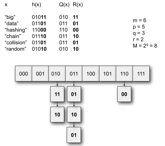
Figure 2.1: Hashing with chaining and quotienting. A quotient filter is a space-efficient implementation (avoiding pointers) of this hashing scheme, see Figure 2.2

The operations on this simplified implementation of the filter work as follows:

• To insert $x$ in the set, we append $R(x)$ to the chain stored in $T[Q(x)]$. Importantly, we allow repetitions of remainders inside the same chain.

• To remove $x$ from the set, we remove one occurrence of $R(x)$ from the chain stored in $T[Q(x)]$.

• To check if $x$ belongs to the set, we check if $R(x)$ appears inside the chain stored in $T[Q(x)]$.

Notice that this scheme allows retrieving $h(x)$ from the table: if remainder $R$ is stored in the $Q$-th chain, then the corresponding fingerprint is $Q\cdot 2^{r}+R$. In other words, the trick is to exploit the location ($Q$) inside the hash table to store information implicitly, in order to reduce the information ($R$) that is explicitly inserted inside the table. This trick was introduced by Knuth in his 1973 book “The Art of Computer Programming: Sorting and Searching”, and already allows to save some space with respect to a classic chained hash that stores the full fingerprints $h(x)$ inside its chains.

Importantly, note that this implementation generates a false positive when we query an element $x$ which is not in the set, and the set contains another element $y\neq x$ with $h(y)=h(y)$. Later we will analyze the false positive probability, which can be reduced by increasing $p$. Note also that, thanks to the fact that we store all occurrences of repeated fingerprints in the table, the data structure does not generate false negatives.

2.3.1 Reducing the space

The QF encodes the table $T$ of the previous subsection using a circular array $H[0,M-1]$ of $M=2^{q}$ slots, each containing an integer of $r+3$ bits: $r$ bits storing a remainder, in addition to the following $3$ metadata bits.

1. is-occupied[i]: this bit records whether there exists an element $x$ in the set such that $i=Q(x)$, i.e. if chain number $i$ contains any remainder.

2. is-shifted[i]: this bit is equal to 0 if and only if the remainder $R(x)$ stored in $H[i]$ corresponds to an element $x$ such that $Q(x)=i$, i.e. if $R(x)$ belongs to the $i$-th chain. In other words, is-shifted[i]=1 indicates that the remainder $R(x)$ stored in $H[i]$ has been shifted to the right w.r.t. its “natural” position $H[Q(x)]$.

3. is-continuation[i]: this bit is equal to 1 if and only if the remainder $R(x)$ stored in $H[i]$ belongs to the same chain of the remainder $R(y)$ stored in $H[i-1]$, i.e. if the two corresponding set elements $x,y$ are such that $Q(x)=Q(y)$.

Figure 2.2 shows the QF implementation of the hash table of Figure 2.1. In this example, the QF uses in total $m\cdot(r+3)=40$ bits (i.e. the bitvector to the right of “Metadata + remainders = QF”).

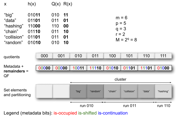
Figure 2.2: Quotient filter encoding of the hash table in Figure 2.1.

While inserting elements, the following invariant is maintained: if $Q(x)<Q(y)$, then $R(x)$ comes before $R(y)$ in the table. We call runs contiguous subsequences corresponding to the same quotient. See Figure 2.2: there are three runs, sorted by their corresponding quotients. We say that a cluster is a maximal contiguous portion $H[i,\dots,j]$ of runs; in particular, $H[i-1]$ and $H[j+1]$ are empty (i.e. do not store any remainder $R(x)$). In Figure 2.2, there is just one cluster (the array $H$ is circular, so that after the cluster there is indeed an empty slot).

It is not hard to see that this implementation allows to simulate chaining. Observe that:

1. Empty cells are those such that $is\_occupied[i]=0$ and $is\_shifted[i]=0$.

2. Runs $H[i,\dots,i+k]$ of the same quotient can be identified because $is\_continuation[i]=0$ and $is\_continuation[i+j]=1$ for all $j=1,\dots,k$.

3. Points (1) and (2) allow us identifying clusters and runs inside a cluster. Looking at all ’1’-bits $is\_occupied[i]=1$ inside a cluster, we can moreover reconstruct which quotients $Q(x)$ are stored inside the cluster. Note also that $R(x)$ is always stored inside the cluster containing cell $H[Q(x)]$.

4. Since quotients in a cluster are sorted and known, and we know their corresponding runs, it is possible to insert/delete/query an element $x$ by scanning the cluster containing position $H[Q(x)]$ (see the original paper [2] for the detailed algorithms).

Point (4) above implies that the average/worst-case query times are asymptotically equal to the average/largest cluster length, respectively.

2.3.2 Analysis

A false positive occurs when we query the QF on an element $x$ not in the set, and $h(x)=h(y)$ for some $y$ in the set ($x\neq y$). Since we assume $h$ to be completely uniform, the probability that $h(x)=h(y)$ is $1/2^{p}$. Then, the probability that $h(x)\neq h(y)$ is $1-1/2^{p}$, thus the probability that $h(x)\neq h(y)$ for all the $m$ elements $y$ in the set is (again by uniformity of $h$) $\left(1-1/2^{p}\right)^{m}$. We conclude that the false positive probability is bounded by

$$1-\left(1-\frac{1}{2^{p}}\right)^{m}=1-\left(1-\frac{1}{2^{p}}\right)^{2^{p}\cdot\frac{m}{2^{p}}}\approx 1-e^{-m/2^{p}}\leq\frac{m}{2^{p}}\leq\frac{2^{q}}{2^{p}}=2^{-r}$$

where the first inequality ($\leq$) follows from the inequality $x\leq\ln\left(\frac{1}{1-x}\right)$ for $x<1$. By setting $\delta=2^{-r}$ (where $0<\delta<1$ is the chosen false positive rate), we obtain that the space used by the QF is $M\cdot(r+3)=M\cdot\log_{2}(1/\delta)+3M$ bits. Recalling that $M=m/\alpha$, where $0<\alpha<1$ is the table’s load factor, we finally obtain that the space is $(m/\alpha)\cdot\log_{2}(1/\delta)+3m/\alpha=O(m\log(1/\delta))$ bits. Notice that this is smaller than the space of the Counting Bloom filter (whose space depends also on the false negative probability $\gamma$; recall that Quotient filters have no false negatives).

The choice of the constant $\alpha$ affects the queries’ running times. In any case, as the following theorem shows, the length of the longest cluster does not exceed $\Theta(\log m)$ with high probability:

Theorem 2.3.1.

For constant load factor $0.5<\alpha<1$ and any constant $c>0$, the probability that the longest cluster exceeds length

$$\frac{3(1+c)\ln M}{1/\alpha+\alpha-2}=\Theta(\log m)$$

is at most $m^{-c}$.

Proof.

If $H[i,\dots,i+k-1]$ is contained in a cluster, then $k$ elements $x_{1},\dots,x_{k}$ in the set are such that $Q(x_{j})\in[i,i+k-1]$ for all $j=1,\dots,k$. For a fixed $x$, the probability that $Q(x)\in[i,i+k-1]$ is $k/M$. Since the hash is fully uniform, the number $C_{i}$ of elements that hash inside $H[i,\dots,i+k-1]$ is the sum of $m$ independent Bernoulli variables $Be(k/M)$. Note that $E[C_{i}]=m\cdot(k/M)=k\alpha$. Applying Lemma 1.2.5 (multiplicative Chernoff), we obtain (note that for $0.5<\alpha<1$ it holds $0<1/\alpha-1<1$ so we can apply the lemma):

$$P(C_{i}=k)=P(C_{i}=(1+(1/\alpha-1))E[C])\leq e^{-k\alpha\cdot(1/\alpha-1)^{2}/3}=e^{-k\cdot(1/\alpha+\alpha-2)/3}$$

So we have $P(H[i,\dots,i+k-1]\mathrm{\ is\ contained\ in\ cluster})\leq e^{-k\cdot(1/\alpha+\alpha-2)/3}$. The longest cluster’s length is greater than or equal to $k$ iff there exists an integer $0\leq i<M$ such that $H[i,\dots,i+k-1]$ is contained in a cluster, so by union bound:

$$P(\mathrm{longest\ cluster\ length}\geq k)\leq M\cdot e^{-k\cdot(1/\alpha+\alpha-2)/3}$$

The above probability is equal to $M^{-c}\leq m^{-c}$ for

$$k=\frac{3(1+c)\ln M}{1/\alpha+\alpha-2}=\Theta(\log m)$$

∎

Moreover, the expected cluster length is a constant:

Theorem 2.3.2.

For constant load factor $0.5<\alpha<1$, the expected cluster length is $O(1)$.

Proof.

If a cluster of length $k$ starts in position $i$, then $C_{i}=k$ so the probability that a particular cluster has length $k$ is at most $e^{-k\cdot(1/\alpha+\alpha-2)/3}$ (see the proof of Theorem 2.3.1). As a result, the expected cluster length is at most $E[C_{i}]$. Using the fact that $\sum_{k=1}^{\infty}k\cdot e^{-kc}=\frac{e^{c}}{(e^{c}-1)^{2}}$, we obtain that, for constant $0.5<\alpha<1$:

$$E[C_{i}]\leq\sum_{k=1}^{\infty}k\cdot e^{-k\cdot(1/\alpha+\alpha-2)/3}\leq\frac{e^{(1/\alpha+\alpha-2)/3}}{(e^{(1/\alpha+\alpha-2)/3}-1)^{2}}\in O(1)$$

See the original paper [2] for a tighter bound as function of $\alpha$. ∎

In practice, choosing $\alpha\in[0.5,0.9]$ guarantees a good space-time trade-off. By choosing $\alpha=0.5$, for example, the space of the filter is $2mr+6m=2m\cdot\log_{2}(1/\delta)+6m$ bits and $99\%$ of the clusters have less than 24 elements (see [2]). This space is slightly larger than that of the Bloom filter, but query times of the QF are much faster: each query requires scanning only one cluster which (due to the average cluster length) will probably fit into a single cache line, thus causing at most one cache miss. Bloom filters, on the other hand, generate one cache miss per hash function used: this makes them several times slower than Quotient filters.

We summarize everything in the following result:

Theorem 2.3.3.

Let $0<\delta<1$ be a user-defined parameter (false positive rate), and let $m$ be a maximum capacity. The Quotient filter supports membership, insert, and delete queries, uses $O\left(m\log(1/\delta)\right)$ bits of space (in addition to the space required to store one fully-independent hash function), and guarantees false positive probability at most $\delta$, provided that no more than $m$ elements are inserted into the filter. The Quotient filter does not generate false negatives. Assuming that the hash function can be evaluated in constant time, all queries take expected $O(1)$ time / worst-case $O(\log m)$ time w.h.p.

Chapter 3 Similarity-preserving sketching

Let $x$ be some data: a set, a string, an integer, etc. A data sketch is the output of a randomized function $f$ (in general, the combination of a certain number of hash functions) mapping $x$ to a sequence of bits $f(x)$ with properties 1-3 below, plus (depending on the application) also property 4:

1. The bit-size of $f(x)$ is much smaller than the bit-size of $x$ (usually, sub-linear or even poly-logarithmic).

2. $f(x)$ can be used to compute (efficiently) some properties of $x$. For example, if $x$ is a multi-set then $f(x)$ could be used to compute an approximation of the number of distinct elements contained in $x$, or the most frequent element in $x$.

3. $f(x)$ can be updated (efficiently) if $x$ gets updated. Importantly, it should be possible to update $f(x)$ without knowing $x$. For example:

   • if we add an element $y$ to a set $x$, it should be possible to compute $f(x\cup\{y\})$ knowing just $f(x)$ and $y$ (not $x$).

   • More in general, given two sketches $f(x_{1})$ and $f(x_{2})$, it should be possible to compute the sketch of the composition of $x_{1}$ and $x_{2}$ (under some operator). For example, if $x_{1}$ and $x_{2}$ are sets we could be interested in obtaining the sketch of $f(x_{1}\cup x_{2})$, without knowing $x_{1}$ and $x_{2}$.

4. If $x$ and $y$ are similar according to some measure of similarity (e.g. Euclidean distance), then $f(x)$ and $f(y)$ are likely to be similar (according to some measure of similarity, not necessarily the same as before).

In this chapter we focus on sketches possessing property 4. In the next chapter we will use sketches to process data streams, focusing more on property 2.

Note that $f(x)$ and $f(y)$ are (in general, dependent) random variables, being $f$ a randomized function.

3.1 Identity - Rabin’s hash function

The most straightforward measure of similarity is identity: is $x$ equal to $y$? Without loss of generality, let $x$ be a string of length $n$ over alphabet $\Sigma=[0,\sigma-1]$; then, we can view strings as integers of $n$ digits in base $\sigma>0$. Note that this setting can also be used to represent subsets of $[1,n]$, letting $\Sigma=\{0,1\}$. Observe that, for any function $f$, if $bitsize(f(x))<bitsize(x)$ (where $bitsize(\cdot)$ is the function returning the number of bits that an object takes in memory) then collisions must occur: there must exist pairs $x\neq y$ such that $f(x)=f(y)$.

The first idea to solve the problem could be to use function $\bar{h}(x)=((a\cdot x+b)\mod M)\mod m$ of Definition 1.3.10: we simply view the string $x$ as a number with $n$ digits in base $|\Sigma|$. Unfortunately, this is not a good idea: recalling that we require $M>x$ for any input $x$ of our function, we would need to perform modular arithmetic on integers with $n$ digits in order to update the sketch!

Rabin’s hashing is a string hashing scheme that solves the above problem (but it cannot achieve universality — even if it guarantees a very low collision probability, see below):

Definition 3.1.1 (Rabin’s hash function [28]).

Fix a prime number $q$, and pick a uniform $z\in[0,q)$. Let $x[1,n]\in\Sigma^{n}$ be a string of length $n$. Rabin’s hash function $\kappa_{q,z}(x)$ is defined as:

$$\kappa_{q,z}(x)=\left(\sum_{i=0}^{n-1}x[n-i]\cdot z^{i}\right)\mod q$$

In other words: $\kappa_{q,z}(x)$ is a polynomial modulo $q$ evaluated in $z$ (a random point in $[0,q)$) and having as coefficients the characters of $x$.

Let $|x|$ denote the length of string $x$. We define the Rabin sketch $f(x)$ of the string $x$ to be the pair

$$f(x)=(\kappa_{q,z}(x),\ z^{|x|}\mod q)$$

Note that $f(x)$ uses just $\Theta(\log q)$ bits.

First, we show that this sketch is easy to compute and update. Suppose we wish to append a character $c$ at the end of $x$, thereby obtaining the string $x\cdot c$ (where $x\cdot c$ means $x$ concatenated with $c$). The hash value of $x$ can be updated as follows (Horner’s method for evaluating polynomials):

Lemma 3.1.2.

$\kappa_{q,z}(x\cdot c)=(\kappa_{q,z}(x)\cdot z+c)\mod q$

The length of $x\cdot c$ is $|x|+1$ and $z^{|x|+1}\mod q=(z^{|x|}\mod q)\cdot z\mod q$.

The above lemma gives us also an efficient algorithm for computing $\kappa_{q,z}(x)$: start from $\kappa_{q,z}(\epsilon)=0$ (where $\epsilon$ is the empty string) and append the characters of $x$ one by one.

Using a similar idea, we can concatenate the sketches of two strings in constant time, as follows:

Lemma 3.1.3.

$\kappa_{q,z}(x\cdot y)=(\kappa_{q,z}(x)\cdot z^{|y|}+\kappa_{q,z}(y))\mod q$

The length of the string $x\cdot y$ is $|x|+|y|$ and the value $z^{|x|+|y|}\mod q$ can be computed efficiently as $z^{|x|+|y|}\mod q=((z^{|x|}\mod q)\cdot(z^{|y|}\mod q))\mod q$.

We prove another important property of Rabin’s hashing: if $x\neq y$, then $\kappa_{q,z}(x)\neq\kappa_{q,z}(y)$ with high probability. This is implied by the following lemma:

Lemma 3.1.4.

Let $x\neq y$, with $\max(|x|,|y|)=n$. Then:

$$P(\kappa_{q,z}(x)=\kappa_{q,z}(y))\leq n/q$$

Proof.

Note that $P(\kappa_{q,z}(x)=\kappa_{q,z}(y))=P(\kappa_{q,z}(x)-\kappa_{q,z}(y)\equiv_{q}0)$. Now, the quantity $\kappa_{q,z}(x)-\kappa_{q,z}(y)$ is, itself, a polynomial. Let $x-y$ be the string such that $(x-y)[i]=x[i]-y[i]\mod q$, where we left-pad with zeros the shortest of the two strings (so that both have $n$ characters). Then, it is easy to see that:

$$\kappa_{q,z}(x)-\kappa_{q,z}(y)\mod q=\kappa_{q,z}(x-y)$$

It follows that the above probability is equal to $P(\kappa_{q,z}(x-y)\equiv_{q}0)$. Since $x\neq y$, $\kappa_{q,z}(x-y)$ is a polynomial of degree at most $n$ over $\mathbb{Z}_{q}$ (evaluated in $z$) and it is not the zero polynomial. Recall that any non-zero univariate polynomial of degree $n$ over a field has at most $n$ roots. Since $q$ is prime, $\mathbb{Z}_{q}$ is a field and thus there are at most $n$ values of $z$ such that $\kappa_{q,z}(x-y)\equiv_{q}0$. Since we pick $z$ uniformly from $[0,q)$, the probability of picking a root is at most $n/q$. ∎

Corollary 3.1.4.1.

Choose a prime $n^{c+1}\leq q\leq 2\cdot n^{c+1}$ for an arbitrarily large constant $c$. Then, $bitsize(\kappa_{q,z}(x))\in O(\log n)$ bits and, for any $x\neq y$:

$$P(\kappa_{q,z}(x)=\kappa_{q,z}(y))\leq n^{-c}$$

that is, $x$ and $y$ collide with low (inverse polynomial) probability.

Later in these notes, Rabin’s hashing will be used to solve pattern matching in the streaming model. As noted above, Rabin hashing can be used also to sketch sets of integers under the following operations (prove it as an exercise):

1. Inserting a new element in the set, provided that the element was not in the set before. This operation can be implemented in $O(\log q)=O(\log n)$ time.

2. Computing the sketch of the union of two disjoint sets in constant time.

3. checking the identity of two sets in constant time.

Observe that, as opposed to the filters of Chapter 2, Rabin hashing allows us to squeeze an arbitrary subset of $[1,n]$ in just $\Theta(\log n)$ bits! The price to pay is that we are limited just to the operations (1-3) above. Since operation (3) can fail with low probability, we are not able to reconstruct the underlying set and therefore we do not break any information-theoretic lower bound.

3.2 Jaccard similarity - MinHash

MinHash is a sketching algorithm used to estimate the similarity of sets. It was invented by Andrei Broder in 1997 and initially used in the AltaVista search engine to detect duplicate web pages and eliminate them from search results.

Here we report just a definition and analysis of MinHash. For more details and applications see Leskovec et al.’s book [21], Sections 3.1 - 3.3.

MinHash is a technique for estimating the Jaccard similarity $J(A,B)$ of two sets $A$ and $B$:

Definition 3.2.1 (Jaccard similarity).

$J(A,B)=\frac{|A\cap B|}{|A\cup B|}$

Without loss of generality, we may assume that we work with sets of integers from the universe $[1,n]$. This is not too restrictive: for example, if we represent a document as the set of all substrings of some length $k$ appearing in it, we can convert those strings to integers using Rabin’s hashing.

Definition 3.2.2 (MinHash hash function).

Let $h$ be a hash function. The MinHash hash function of a set $A$ is defined as $\hat{h}(A)=\min\{h(x)\ :\ x\in A\}$, i.e. it is the minimum of $h$ over all elements of $A$.

Definition 3.2.3 (MinHash estimator).

Let $\hat{J}_{h}(A,B)$ be the indicator R.V. defined as follows:

$$\hat{J}_{h}(A,B)=\begin{cases*}1&if $\hat{h}(A)=\hat{h}(B)$\\ 0&otherwise\end{cases*}$$ (3.1)

Note that $\hat{J}_{h}(A,B)$ is a Bernoullian R.V. We prove the following remarkable property:

Lemma 3.2.4.

If $h:[1,n]\rightarrow[1,n]$ is a uniform permutation, then $E[\hat{J}_{h}(A,B)]=J(A,B)$

Proof.

Let $|A\cup B|=N$. For $i\in A\cup B$, consider the event $smallest(i)=(\forall j\in A\cup B-\{i\})(h(i)<h(j))$, stating that $i$ is the element of $A\cup B$ mapped to the smallest hash $h(i)$ (among all elements of $A\cup B$). Since $h$ is a permutation, exactly one element from $A\cup B$ will be mapped to the smallest hash (i.e. $smallest(i)$ is true for exactly one $i\in A\cup B$), so $\{smallest(i)\}_{i\in A\cup B}$ is a partition of cardinality $N=|A\cup B|$ of the event space. Moreover, the fact that $h$ is completely uniform implies that $P(smallest(i))=P(smallest(j))$ for all $i,j\in A\cup B$: every element of $A\cup B$ has the same chance to be mapped to the smallest hash (among elements of $A\cup B$). This implies that $P(smallest(i))=1/N$ for every $i\in A\cup B$.

Note that, if we know that $smallest(i)$ is true and $i\in A\cap B$, then $\hat{J}_{h}(A,B)=1$ (because $i$ belongs to both $A$ and $B$ and $h$ reaches its minimum $\mathtt{min}$ on $i$, thus $\hat{h}(A)=\hat{h}(B)=\mathtt{min}$). On the other hand, if we know that $smallest(i)$ is true and $i\in(A\cup B)-(A\cap B)$, then $\hat{J}_{h}(A,B)=0$ (because $i$ belongs to either $A$ or $B$ — not both — and $h$ reaches its minimum $\mathtt{min}$ on $i$, thus either $\hat{h}(A)\neq\hat{h}(B)=\mathtt{min}$ or $\mathtt{min}=\hat{h}(A)\neq\hat{h}(B)$ holds).

Using this observation and applying the law of total expectation (Lemma 1.1.11) to the partition $\{smallest(i)\}_{i\in A\cup B}$ of the event space we obtain:

$$\begin{array}[]{ccl}E[\hat{J}_{h}(A,B)]&=&\sum_{i\in A\cup B}P(smallest(i))\cdot E[\hat{J}_{h}(A,B)\ |\ smallest(i)]\\ &=&\sum_{i\in A\cup B}\frac{1}{N}\cdot E[\hat{J}_{h}(A,B)\ |\ smallest(i)]\\ &=&\sum_{i\in A\cap B}\frac{1}{N}\cdot E[\hat{J}_{h}(A,B)\ |\ smallest(i)]+\sum_{i\in(A\cup B)-(A\cap B)}\frac{1}{N}\cdot E[\hat{J}_{h}(A,B)\ |\ smallest(i)]\\ &=&\sum_{i\in A\cap B}\frac{1}{N}\cdot 1+\sum_{i\in(A\cup B)-(A\cap B)}\frac{1}{N}\cdot 0\\ &=&\frac{1}{N}\cdot\sum_{i\in A\cap B}1\\ &=&\frac{1}{N}|A\cap B|\\ &=&\frac{|A\cap B|}{|A\cup B|}\\ &=&J(A,B)\end{array}$$

∎

The above lemma states that $\hat{J}_{h}(A,B)$ is an unbiased estimator for the Jaccard similarity. Note that evaluating the estimator only requires knowledge of $\hat{h}(A)$ and $\hat{h}(B)$: an entire set is squeezed down to just one integer!

3.2.1 Min-wise independent permutations

The main drawback of the previous approach is that $h$ is a random permutation. There are $n!$ random permutations of $[1,n]$, so $h$ requires $\log_{2}(n!)\in\Theta(n\log n)$ bits to be stored. What property of $h$ makes the proof of Lemma 3.2.4 work? It turns out that we need the following:

Definition 3.2.5 (Min-wise independent hashing).

Let $h:[1,n]\rightarrow[0,M)$ be a function from some family $\mathcal{H}$. For any subset $A\subseteq[0,M)$ and $i\in A$, let $smallest_{h}(A,i)=(\forall j\in A-\{i\})(h(i)<h(j))$.

The family $\mathcal{H}$ is said to be min-wise independent if, for a uniform $h\in\mathcal{H}$, $P(smallest_{h}(A,i))=1/|A|$ for any $A\subseteq[1,n]$ and $i\in A$.

In other words, $\mathcal{H}$ is min-wise independent if, for any subset of the domain, any element is equally likely to be the minimum (through a uniform $h\in\mathcal{H}$). The definition could be made more general by further relaxing the uniformity requirement on $h$.

Unfortunately, Broder et al. [4] proved that any family of min-wise independent permutations must include at least $e^{n-o(n)}$ permutations, so a min-wise independent function requires at least $n\log_{2}e\approx 1.44n$ bits to be stored. This lower bound is easy to prove. First, observe that any $h\in\mathcal{H}$ identifies exactly one minimum in $A$. Since every $i\in A$ should have the same probability to be mapped to the minimum through a uniform $h\in\mathcal{H}$, it follows that $|A|$ must necessarily divide $|\mathcal{H}|$. This should hold for every $A\subseteq[1,n]$, so each $k=1,2,\dots,n$ should divide $|\mathcal{H}|$ and therefore $|\mathcal{H}|$ cannot be smaller than the least common multiple of all numbers $1,2,\dots,n$. The claim follows from the fact that $lcm(1,2,\dots,n)=e^{n-o(n)}$.

There are two solutions to this problem:

1. (k-min-wise independent hashing) We require $P(smallest_{h}(A,i))=1/|A|$ only for sets of cardinality $|A|\leq k$.

2. (Approximate min-wise hashing): we require $P(smallest_{h}(A,i))=(1\pm\epsilon)/|A|$ for a small error $\epsilon>0$.

Also combinations of (1) and (2) are possible. A hash with property (1) can be stored in $O(k)$ bits of space and is a good compromise: in practice, $k$ is the cardinality of the union of the two largest sets in our dataset (much smaller than the universe’s size $n$). As far as solution (2) is concerned, there exist hash functions of size $\Theta(\log(1/\epsilon)\cdot\log n)$ bits with this property. Such functions can be used to estimate the Jaccard similarity with absolute error $\epsilon$. For more details, see [19, 27].

3.2.2 Reducing the variance

The R.V. $\hat{J}_{h}(A,B)$ of Definition 3.2.3 is not a good estimator since it is a Bernoullian R.V. and thus has a large variance: in the worst case ($J(A,B)=0.5$), we have $Var[\hat{J}_{h}(A,B)]=0.25$ and thus the expected error (standard deviation) of $\hat{J}_{h}(A,B)$ is $\sqrt{Var[\hat{J}_{h}(A,B)]}=0.5$. This means that on expectation we are off by $50\%$ from the true value of $J(A,B)$. We know how to solve this issue: just take the average of $k$ independent such estimators, for sufficiently large $k$.

Let $h_{i}:[1,n]\rightarrow[1,n]$, with $i=1,\dots,k$, be $k$ independent uniform permutations. We define the MinHash sketch of a set $A$ to be the $k$-tuple:

Definition 3.2.6 (MinHash sketch).

$h_{min}(A)=(\hat{h}_{1}(A),\hat{h}_{2}(A),\dots,\hat{h}_{k}(A))$

In other words: the $i$-th element of $h_{min}(A)$ is the smallest hash $h_{i}(x)$, for $x\in A$. Note that the MinHash sketch of a set $A$ can be easily computed in $O(k|A|)$ time, provided that $h$ can be evaluated in constant time. Then, we estimate $J(A,B)$ using the following estimator:

Definition 3.2.7 (Improved MinHash estimator).

$$J^{+}(A,B)=\frac{1}{k}\sum_{i=1}^{k}\hat{J}_{h_{i}}(A,B)$$

In other words, we compute the average of $\hat{J}_{h_{i}}(A,B)$ for $i=1,\dots,k$. Note that the improved MinHash estimator can be computed in $O(k)$ time given the MinHash sketches of two sets.

We can immediately apply the double-sided additive Chernoff-Hoeffding bound (Lemma 1.2.4) and obtain that $P(|J^{+}(A,B)-J(A,B)|\geq\epsilon)\leq 2e^{-\epsilon^{2}k/2}$ for any desired absolute error $0<\epsilon\leq 1$. Fix now any desired failure probability $0<\delta\leq 1$. By solving $2e^{-\epsilon^{2}k/2}=\delta$ we obtain $k=2\ln(2/\delta)/\epsilon^{2}$. We can finally state:

Theorem 3.2.8.

Fix any desired absolute error $0<\epsilon\leq 1$ and failure probability $0<\delta\leq 1$. By using $k=\frac{2}{\epsilon^{2}}\ln(2/\delta)\in O\left(\frac{\log(1/\delta)}{\epsilon^{2}}\right)$ hash functions, the estimator $J^{+}(A,B)$ exceeds absolute error $\epsilon$ with probability at most $\delta$, i.e.

$$P(|J^{+}(A,B)-J(A,B)|\geq\epsilon)\leq\delta$$

To summarize, we can squeeze down any subset of $[1,n]$ to a MinHash sketch of $O\left(\frac{\log(1/\delta)}{\epsilon^{2}}\log n\right)$ bits so that, later, in $O\left(\frac{\log(1/\delta)}{\epsilon^{2}}\right)$ time we can estimate the Jaccard similarity between any pair of sets (represented with MinHash sketches) with arbitrarily small absolute error $\epsilon$ and arbitrarily small failure probability $\delta$.

Note that it is easy to combine the MinHash sketches of two sets $A$ and $B$ so to obtain the MinHash sketch of $A\cup B$ (similarly, to compute the MinHash sketch of $A\cup\{x\}$ given the MinHash sketch of $A$): $h_{min}(A\cup B)=(\min\{\hat{h}_{1}(A),\hat{h}_{1}(B)\},\dots,\min\{\hat{h}_{k}(A),\hat{h}_{k}(B)\})$.

3.3 Hamming distance

We devise a simple sketching mechanism for Hamming distance. Given two strings $x,y\in\Sigma^{n}$ of the same length $n$, the Hamming distance $d_{H}(x,y)$ is the number of positions where $x$ and $y$ differ:

$$d_{H}(x,y)=\sum_{i=1}^{n}(x[i]\neq y[i])$$

where $(x[i]\neq y[i])=1$ if $x[i]\neq y[i]$, and 0 otherwise. Since $d_{H}$ is defined for strings of the same length $n$, we may scale it to a real number in $[0,1]$ as follows: $d^{\prime}_{H}(x,y)=d_{H}(x,y)/n$. Note that two strings are equal if and only if $d^{\prime}_{H}(x,y)=0$ ($d^{\prime}_{H}(x,y)$ is indeed a metric, see next section).

If $n$ is large, also the Hamming distance admits a simple sketching mechanism. Choose a uniform $i\in[1,n]$ and define

$$h_{i}(x)=x[i]$$

Then, it is easy to see that $P(h_{i}(x)\neq h_{i}(y))=d^{\prime}_{H}(x,y)$. Similarly to the Jaccard case, we can define an indicator R.V.

$$\hat{H}_{i}(x,y)=\begin{cases*}1&if $h_{i}(x)\neq h_{i}(y)$\\ 0&otherwise\end{cases*}$$ (3.2)

and obtain $E[\hat{H}_{i}(x,y)]=d^{\prime}_{H}(x,y)$. Again, this indicator is Bernoullian and has a large variance. To reduce the variance, we can pick $k$ uniform indices $i_{1},\dots,i_{k}\in[1,n]$ and define an improved indicator:

$$H^{+}(x,y)=\frac{1}{k}\sum_{j=1}^{k}\hat{H}_{i_{j}}(x,y)$$

Applying Chernoff-Hoeffding:

Theorem 3.3.1.

Fix an absolute error $0\leq\epsilon\leq 1$ and failure probability $0<\delta\leq 1$. By using $k=\frac{2}{\epsilon^{2}}\ln(2/\delta)\in O\left(\frac{\log(1/\delta)}{\epsilon^{2}}\right)$ hash functions, the estimator $H^{+}(x,y)$ exceeds absolute error $\epsilon$ with probability at most $\delta$, i.e.

$$P(|H^{+}(x,y)-d^{\prime}_{H}(x,y)|\geq\epsilon)\leq\delta$$

Note that the family of hash functions $\{h_{i}\ |\ 1\leq i\leq n\}$ contains only $n$ elements. This number is much smaller than the $n!$ permutations of the Jaccard case. If the goal is just to compare sketches this is not an issue: as the number $O\left(\frac{\log(1/\delta)}{\epsilon^{2}}\right)$ of hash functions approaches $n$, the accuracy of our estimator increases since we are including most of the string’s characters in the sketch (the extreme case is when all characters are included: then, the sketch allows computing the Hamming distance exactly and with success probability 1).

3.4 Other metrics

In general, a sketching scheme can be devised for most distance metrics. A distance metric over a set $A$ is a function $d:A\times A\rightarrow\mathbb{R}$ with the following properties:

• Non-negativity: $d(x,y)\geq 0$

• Identity: $d(x,y)=0$ iff $x=y$

• Simmetry: $d(x,y)=d(y,x)$

• Triangle inequality: $d(x,z)\leq d(x,y)+d(y,z)$

For example, the Jaccard distance $d_{J}(x,y)=1-J(x,y)$ defined over sets is indeed a distance metric (exercise: prove it). Of course, the sketching mechanism we devised for Jaccard similarity works for Jaccard distance without modifications (just invert the definition of the estimator of Definition 3.2.3). Some examples of distances among vectors $x,y\in\mathbb{R}^{d}$ are:

• $L_{p}$ norm (or Minkowski distance): $L_{p}(x,y)=\left(\sum_{i=1}^{d}|x_{i}-y_{i}|^{p}\right)^{1/p}$

• $L_{2}$ norm (or Euclidean distance): $L_{2}(x,y)=\sqrt{\sum_{i=1}^{d}(x_{i}-y_{i})^{2}}$

• $L_{1}$ norm (or Manhattan distance): $L_{1}(x,y)=\sum_{i=1}^{d}|x_{i}-y_{i}|$

• $L_{\infty}$ norm: $L_{\infty}(x,y)=\max\{|x_{1}-y_{1}|,\dots,|x_{d}-y_{d}|\}$

• Cosine distance: $d_{cos}(x,y)=1-cos(x,y)=1-\frac{x\cdot y}{\lVert x\rVert\cdot\lVert y\rVert}=1-\frac{\sum_{i=1}^{d}x_{i}y_{i}}{\sqrt{\sum_{i=1}^{d}x_{i}^{2}}\cdot\sqrt{\sum_{i=1}^{d}y_{i}^{2}}}$

Between strings, we have:

• Hamming distance between two equal-length strings: $H(s_{1},s_{2})$ is the number of positions $s_{1}[i]\neq s_{2}[i]$ in which the two strings differ. On alphabet $\{0,1\}$ it is equal to $L_{1}(s_{1},s_{2})$.

• Edit distance between any two strings: $Ed(s_{1},s_{2})$ is the minimum number of edits (substitutions, single-character inserts/deletes) that have to be applied to $s_{1}$ in order to convert it into $s_{2}$.

3.5 Locality-sensitive hashing (LSH)

Suppose our task is to find all similar pairs of elements (small $d(x,y)$) in a data set $A\subseteq U$ ($U$ is some universe). While a distance-preserving sketch (e.g. for Jaccard distance) speeds up the computation of $d(x,y)$, we still need to compute $O(|A|^{2})$ distances in order to find all similar pairs! On big data sets this is clearly not feasible.

Locality-sensitive hash functions are used to accelerate the search of similar elements in a data set, where similarity is usually measured in terms of a distance metric. The main intuition behind LSH is that similar items are likely to be hashed to the same value.

3.5.1 The theory of LSH

A locality-sensitive hash function for some distance metric $d:U\times U\rightarrow\mathbb{R}$ is a function $h:U\rightarrow[0,M)$ such that similar elements (i.e. $d(x,y)$ is small) are likely to collide: $h(x)=h(y)$. This is useful to drastically reduce the search space with the following algorithm:

1. Scan the data set $A$ and put each element $x\in A$ in bucket $H[h(x)]$ of a hash table $H$.

2. Compute distances only between pairs inside each bucket $H[i]$.

Classic hash data structures use $O(m)$ space for representing a set of $m$ elements and support insertions and lookups in $O(1)$ expected time (see Section 1.3.4). More advanced data structures support queries in $O(1)$ worst-case time with high probability. In the following, we will therefore assume constant-time operations for our hash data structures.

LSH works by first defining a distance threshold $t$. Ideally, we would like the collision probability to be equal to 0 for pairs such that $d(x,y)>t$ and equal to 1 for pairs such that $d(x,y)\leq t$. For example, using a distance $d:U\times U\rightarrow[0,1]$ (e.g. Jaccard distance) the ideal LSH function should be the one depicted in Figure 3.1.

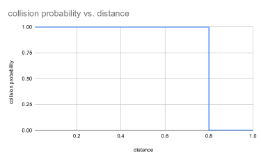
Figure 3.1: The ideal locality-sensitive hash function: elements whose distance is below the threshold $t=0.8$ collide with probability 1; elements whose distance is above the threshold do not collide.

In practice, we are happy with a good approximation:

Definition 3.5.1.

A $(d_{1},d_{2},p_{1},p_{2})$-sensitive family $\mathcal{H}$ of hash functions is such that, for a uniformly-chosen $g\in\mathcal{H}$, we have:

• If $d(x,y)\leq d_{1}$, then $P(g(x)=g(y))\geq p_{1}$.

• If $d(x,y)\geq d_{2}$, then $P(g(x)=g(y))\leq p_{2}$.

Intuitively, we want $d_{1}$ and $d_{2}$ to be as close as possible ($d_{1}\leq d_{2}$), $p_{1}$ as large as possible, and $p_{2}$ as small as possible. To abbreviate, in the following we will say that $h$ is a $(d_{1},d_{2},p_{1},p_{2})$-sensitive hash function when it is uniformly drawn from a $(d_{1},d_{2},p_{1},p_{2})$-sensitive family. For example, Figure 3.3 shows the behaviour of a $(0.4,0.7,0.999,0.007)$-sensitive hash function for Jaccard distance (see next subsection for more details).

We now show how locality-sensitive hash functions can be amplified in order to obtain different (better) parameters.

AND construction

Suppose $\mathcal{H}$ is a $(d_{1},d_{2},p_{1},p_{2})$-sensitive family. Pick uniformly $r$ independent hash functions $h_{1},\dots,h_{r}\in\mathcal{H}$, and define:

Definition 3.5.2 (AND construction).

$h^{AND}(x)=(h_{1}(x),\dots,h_{r}(x))$

Then, if two elements $x,y\in U$ collide with probability $p$ using any of the $h_{i}$, now they collide with probability $p^{r}$ using $h^{AND}$ (because the $h_{i}$ are independent). In other words, the curve becomes $P(collision)=p^{r}$ and we conclude:

Lemma 3.5.3.

$h^{AND}$ is a $(d_{1},d_{2},p_{1}^{r},p_{2}^{r})$-sensitive hash function.

Observe that, if the output of $h$ is one integer, then $h^{AND}$ outputs $r$ integers. However, we may use one additional collision-free hash function $h^{\prime}$ to reduce this size to one integer: $x$ is mapped to $y=h^{\prime}(h^{AND}(x))$. This is important, since later we will need to insert $y$ in a hash table (this trick reduces the space by a factor of $r$).

OR construction

Suppose $\mathcal{H}$ is a $(d_{1},d_{2},p_{1},p_{2})$-sensitive family. Pick uniformly $b$ independent hash functions $h_{1},\dots,h_{b}\in\mathcal{H}$, and define:

Definition 3.5.4 (OR construction).

We say that $x$ and $y$ collide iff $h_{i}(x)=h_{i}(y)$ for at least one $1\leq i\leq b$.

Note: the OR construction can be simulated by simply keeping $b$ hash tables $H_{1},\dots,H_{b}$, and inserting $x$ in bucket $H_{i}[h_{i}(x)]$ for each $1\leq i\leq b$. Then, two elements collide iff they end up in the same bucket in at least one hash table.

Suppose two elements $x,y\in U$ collide with probability $p$ using any hash function $h_{i}$. Then:

• For a fixed $i$, we have that $P(h_{i}(x)\neq h_{i}(y))=1-p$

• The probability that all hashes do not collide is $P(\wedge_{i=1}^{b}h_{i}(x)\neq h_{i}(y))=(1-p)^{b}$

• The probability that at least one hash collides is

  $$P(\vee_{i=1}^{b}h_{i}(x)=h_{i}(y))=1-P(\wedge_{i=1}^{b}h_{i}(x)\neq h_{i}(y))=1-(1-p)^{b}$$

We conclude that the OR construction yields a curve of the form $P(collision)=1-(1-p)^{b}$ so:

Lemma 3.5.5.

The OR construction yields a $(d_{1},d_{2},1-(1-p_{1})^{b},1-(1-p_{2})^{b})$-sensitive hash function.

Combining AND+OR

By combining the two constructions, each $x$ is hashed through $rb$ hash functions: we keep $b$ hash tables and insert each $x\in U$ in buckets $H_{i}[h^{AND}_{i}(x)]$ for each $1\leq i\leq b$, where $h^{AND}_{i}$ is the combination of $r$ independent hash values. We obtain:

Lemma 3.5.6.

If $\mathcal{H}$ is a $(d_{1},d_{2},p_{1},p_{2})$-sensitive family, then the AND+OR constructions with parameters $r$ and $b$ yields a $(d_{1},d_{2},1-(1-p_{1}^{r})^{b},1-(1-p_{2}^{r})^{b})$-sensitive family.

It turns out (see next subsections) that by playing with parameters $r$ and $b$ we can obtain a function as close as we wish to the ideal LSH of Figure 3.1.

3.5.2 LSH for Jaccard distance

Let $\hat{h}$ be the MinHash function of Definition 3.2.2. In Section 3.2 we have established that $P(\hat{h}(A)=\hat{h}(B))=J(A,B)$, i.e. the probability that two elements collide through $\hat{h}$ is exactly their Jaccard similarity. Recall that we have defined the Jaccard distance (a metric) to be $d_{J}(A,B)=1-J(A,B)$. But then, $P(\hat{h}(A)=\hat{h}(B))=1-d_{J}(A,B)$ and we obtain that $\hat{h}$ is a $(d_{1},d_{2},1-d_{1},1-d_{2})$-sensitive hash function for any $0\leq d_{1}\leq d_{2}\leq 1$, see Figure 3.2.

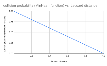
Figure 3.2: The MinHash function $\hat{h}$ of Definition 3.2.2 is a $(d_{1},d_{2},1-d_{1},1-d_{2})$-sensitive function for any $0\leq d_{1}\leq d_{2}\leq 1$.

Using the AND+OR construction, we can amplify $\hat{h}$ and obtain a $(d_{1},d_{2},1-(1-(1-d_{1})^{r})^{b},1-(1-(1-d_{2})^{r})^{b})$-sensitive function for any $0\leq d_{1}\leq d_{2}\leq 1$. For example, with $r=10$ and $b=1200$ we obtain a function whose behaviour is depicted in Figure 3.3.

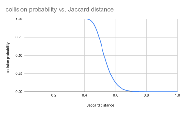
Figure 3.3: A $(0.4,0.7,0.999,0.007)$-sensitive hash function for Jaccard distance built with AND+OR construction with parameters $r=10$ and $b=1200$ starting from a $(0.4,0.7,0.6,0.3)$-sensitive LSH function. Equivalently, we can take two closer points $d_{1}$ and $d_{2}$ on the curve: for example, this function is also $(0.5,0.6,0.69,0.12)$-sensitive.

The shape of the s-curve is dictated by the parameters $b$ and $r$. As it turns out, $b$ controls the steepness of the slope, that is, the distance between the two points where the probability becomes close to 0 and close to 1. The larger $b$, the steeper the s-curve is. In other words, $b$ controls the distance between $d_{1}$ and $d_{2}$ in our LSH: we want $b$ to be large. Parameter $r$, on the other hand, controls the position of the slope (the point where the curve begins to decrease).

Let $p$ be the collision probability and $d_{J}$ be the Jaccard distance. The s-curve follows the equation $p=1-(1-(1-d_{J})^{r})^{b}$ By observing that the center of the slope is approximately around $p=1/2$, one can determine the parameters $b$ and $r$ as a function of the slope position $d_{J}$. Let’s solve the following equation as a function of $r$:

$$1-(1-(1-d_{J})^{r})^{b}=1/2$$

We obtain (note that $r$ should be an integer so we must approximate somehow):

$$r=\left\lfloor\frac{\ln\left(1-2^{-1/b}\right)}{\ln(1-d_{J})}\right\rfloor$$

The fact that we have to approximate $r$ to an integer means that the slope of the resulting curve will not be centered exactly at $d_{J}$. By playing with parameter $b$, one can further adjust the curve.

Example 3.5.7.

Suppose we want to build a LSH to identify sets with Jaccard distance at most $0.9$. We choose a large $b=100000$. Then, the above equation gives us $r=\left\lfloor\frac{\ln\left(1-2^{-1/100000}\right)}{\ln(1-0.9)}\right\rfloor=5$. Using these parameters, we obtain the LSH shown in Figure 3.4. For example, one can extract two data points from this curve and see that this is a $(0.85,0.95,0.99949,0.03076)$-sensitive function.

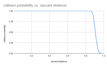
Figure 3.4: LSH built for Example 3.5.7.

Clearly, a large $b$ has a cost: in Example 3.5.7, we have to compute $r\cdot b=5\cdot 10^{5}$ MinHash functions for each set, which means that we have to apply $5\cdot 10^{5}$ basic hash functions $h$ (see Definition 3.2.2) to each element of each set. Letting $t=r\cdot b$, this translates to $O(|A|\cdot t)$ running time for a set $A$. Dahlgaard et al. [9] improved this running time to $O(|A|+t\log t)$. Another solution is to observe that the $t$ MinHashes are completely independent, thus their computation can be parallelized optimally (for example, with a MapReduce job running over a large cluster).

Observe also that a large value of $b$ requires a large family of hash functions. While this is not a problem with the Jaccard distance (where the supply of $n!$ permutations is essentially unlimited), it could be a problem with the sketch for Hamming distance presented in Section 3.3. There, we could choose only among $n$ hash functions, $n$ being the strings’ length. It follows that the resulting LSH scheme is not good for small strings (small $n$).

3.5.3 Nearest neighbour search

One application of LSH is nearest neighbour search:

Definition 3.5.8 (Nearest neighbour search (NNS)).

For a given distance threshold $D$, preprocess a data set $A$ of size $|A|=m$ in a data structure such that later, given any data point $x$, we can quickly find a point $y\in A$ such that $d(x,y)\leq D$.

To solve the NNS problem, let $\mathcal{H}$ be a $(D^{\prime},D,p_{1},p_{2})$-sensitive family, with $D^{\prime}$ as close as possible to (and smaller than) $D$. Suppose moreover that $h(x)$ can be evaluated in time $t_{h}$ (this time is proportional to the size/cardinality of $x$) and $d(x,y)$ can be computed in time $t_{d}$. Note that $t_{d}$ can be reduced considerably by employing sketches — see Section 3.2. We amplify $\mathcal{H}$ with an AND+OR construction with parameters $r$ (AND) and $b$ (OR). Our data structure is formed by $b$ hash tables $H_{1},\dots,H_{b}$. For each of the $m$ data points $x\in A$, we compute the $b$ functions $h^{AND}_{i}(x)$ in total time $O(m\cdot b\cdot r\cdot t_{h})$ and insert in $H_{i}[h^{AND}_{i}(x)]$ a pointer to the original data point $x$ (or to its sketch). Assuming that a hash table storing $m$ pointers occupies $O(m)$ words of space and can be constructed in (expected) $O(m)$ time, we obtain:

Lemma 3.5.9.

Our NNS data structure can be constructed in $O(m\cdot b\cdot r\cdot t_{h})$ time and occupies $O(m\cdot b)$ space (in addition to the original data points — or their sketches).

To answer a query $x$, note that we are interested in finding just one point $y$ such that $d(x,y)\leq D$: we can stop our search as soon as we find one. In $O(t_{h}\cdot b\cdot r)$ time we compute the hashes $h^{AND}_{i}(x)$ for all $1\leq i\leq b$. In the worst case, all the $m$ data points $y$ are such that $d(x,y)>D$. The probability that one such point ends up in bucket $H_{i}[h^{AND}_{i}(x)]$ is at most $p_{2}^{r}$. As a result, the expected number of false positives in each bucket $H_{i}[h^{AND}_{i}(x)]$ is at most $m\cdot p_{2}^{r}$; in total, this yields $m\cdot b\cdot p_{2}^{r}$ false positives that need to be checked against $x$. For each of these false positives, we need to compute a distance in time $t_{d}$. We obtain:

Lemma 3.5.10.

Let:

• $FP=m\cdot b\cdot p_{2}^{r}$ be the expected number of false positives in the worst case.

• $T=b\cdot r$ be the total number of independent hash functions used by our structure.

Our NNS data structure answers a query in expected time $O(t_{h}\cdot T+FP\cdot t_{d})$. If there exists a point within distance at most $D^{\prime}$ from our query, then we return an answer with probability at least $1-(1-p_{1}^{r})^{b}$.

Example 3.5.11.

Consider the $(0.4,0.7,0.999,0.007)$-sensitive family of Figure 3.3. This function has been built with AND+OR construction with parameters $r=10$ and $b=1200$ taking as starting point the $(0.4,0.7,0.6,0.3)$-sensitive hash function of Figure 3.3 (in fact, $1-(1-0.6^{r})^{b}\approx 0.999$ and $1-(1-0.3^{r})^{b}\approx 0.007$). We can therefore use this hash to solve the NNS problem with threshold $D=0.7$. Lemma 3.5.10 states that at most $FP=m\cdot b\cdot p_{2}^{r}\approx 0.007\cdot m$ false positives need to be explicitly checked against our query (compare this with a naive strategy that compares $100\%$ of the $m$ points with the query). Moreover, if at least one point within distance $D^{\prime}=0.4$ from our query exists, we will return a point within distance $0.4$ with probability at least $1-(1-0.6^{r})^{b}\approx 0.999$. The data structure uses space proportional to $b=1200$ words (a few kilobytes) for each data point; note that, in big data scenarios, each data point (for example, a document) is likely to use much more space than that so this extra space is negligible.

Chapter 4 Mining data streams

A data stream is a sequence $x=x_{1},x_{2},\dots,x_{m}$ of elements (without loss of generality, integers from the range $[1,n]$). We receive these elements one at a time, from $x_{1}$ to $x_{m}$. Typically, $m$ is too large and we cannot keep all the stream in memory. The goal of streaming algorithms is to compute useful statistics on the stream while using as little memory as possible (usually, poly-logarithmic in $m$ and $n$).

A streaming algorithm is evaluated on these parameters:

1. Memory used (as a function of, e.g., stream length $m$ and universe size $n$).

2. Delay per element: the worst-case time taken by the algorithm to process each stream element.

3. Probability of obtaining a correct solution or a good approximation of the correct result.

4. Approximation ratio (e.g. the value returned by the algorithm is a $(1\pm\epsilon)$ approximation of the correct answer, for a small $\epsilon\geq 0$).

A nice introduction to data sketching and streaming is given in [8].

4.1 Pattern matching

The first example of stream statistic we consider is pattern matching. Say the elements $x_{i}$ belong to some alphabet $\Sigma$: the stream is a string of length $m$ over $\Sigma$. Suppose we are given a pattern $y=y_{1}y_{2}\dots y_{n}\in\Sigma^{n}$. The pattern’s length $n$ is smaller than $m$, but also $n$ could be very large (so that $y$ too does not fit in memory or cache). The question we tackle in this section is: how many times does $y$ appear in $x$ as a substring $y=x_{i}x_{i+1}\dots x_{i+n-1}$?

Example 4.1.1 (Intrusion Detection and Prevention Systems (IDPSs)).

IDPSs are software tools that scan network traffic in search of known patterns such as virus fragments or malicious code. The searched patterns are usually very numerous, so the memory usage and delay of the used pattern matching algorithm is critical. Ideally, the algorithm should work entirely in cache in order to achieve the best performance. See also the paper [17].

4.1.1 Karp-Rabin’s algorithm

Rabin’s hashing is the main tool we will use to solve the problem. First, we note that the technique itself yields a straightforward solution, even though in $O(n)$ space. In the next section we refine this solution to use $O(\log n)$ space.

Suppose we have processed the stream up to $x_{1},\dots,x_{i}$ ($i\geq n$) and that we know the hash values $\kappa_{q,z}(x_{i-n+1}x_{i-n+2}\dots x_{i})$ and $\kappa_{q,z}(y)$. By simply comparing these two hash values (in constant time) we can discover whether or not the patter occurs in the last $n$ stream’s characters. The crucial step is to update the hash of the stream when a new element $x_{i+1}$ arrives. This is not too hard: we have to subtract character $x_{i-n+1}$ from the stream’s hash and add the new character $x_{i+1}$. This can be achieved as follows:

$$\kappa_{q,z}(x_{i-n+2}x_{i-n+2}\dots x_{i+1})=(\kappa_{q,z}(x_{i-n+1}x_{i-n+2}\dots x_{i})-x_{i-n+1}\cdot z^{n-1})\cdot z+x_{i+1}\mod q$$

The value $z^{n-1}\mod q$ can be pre-computed, so the above operation takes constant time. Note that, since we need to access character $x_{i-n+1}$, at any time the algorithm must keep the last $n$ characters seen in the stream, thereby using $O(n)$ space.

Analysis

Note that, if there are no collisions between the pattern and all the $m-n+1\leq m$ stream’s substrings of length $n$, then the algorithm returns the correct result (number of occurrences of the pattern in the stream). From Section 3.1, the probability that the pattern collides with any of those substrings is at most $n/q$. By union bound, the probability that the patter collides with at least one substring is $mn/q\leq m^{2}/q$. We want this to happen with small (inverse polynomial probability): this can be achieved by choosing a prime $q$ in the range $[m^{c+2},2\cdot m^{c+2}]$, for any constant $c$. Such a prime (and therefore the output of Rabin’s hash function) can be stored in $O(\log m)$ bits = $O(1)$ words. We obtain:

Theorem 4.1.2.

The Karp-Rabin algorithm solves the pattern matching problem in the streaming model using $O(n)$ words of memory and $O(1)$ delay. The correct solution is returned with high (inverse-polynomial) probability $1-m^{-c}$, for any constant $c\geq 1$ chosen at initialization time.

There exist also deterministic algorithms with $O(1)$ delay and $O(n)$ space. However, as we show in the next section, Karp-Rabin’s randomization enables an exponentially more space-efficient solution.

4.1.2 Porat-Porat’s algorithm

The big disadvantage of Karp-Rabin’s algorithm is that it uses too much memory: $O(n)$ words per pattern. In this section we study an algorithm described by Benny Porat and Ely Porat in [26] that uses just $O(\log n)$ words of space and has $O(\log n)$ delay per stream’s character . Other algorithms are able to reduce the delay to the optimal $O(1)$ (see [3]). For simplicity, assume that $n$ is a power of two: $n=2^{e}$ for some $e\geq 0$. The algorithm can be generalized to any $n$ in a straightforward way. The overall idea is to:

• Keep a counter $occ$ initialized to $0$, storing the number of occurrences of $y$ found in $x$.

• Keep the hashes of all $1+e=1+\log_{2}n$ prefixes of $y$ whose length is a power of two.

• Keep the occurrences of those prefixes of $y$ on the stream, working in $e$ levels: level $0\leq i<e$ records all occurrences of the prefix $y[1,2^{i}]$ in a window containing the last $2^{i+1}$ stream’s characters. Using a clever argument based on string periodicity, show that this information can be ”compressed” in just $O(1)$ space per level ($O(\log n)$ space in total).

• Before the new character $x_{j}$ arrives: for every level $i>0$, if position $p=j-2^{i+1}$ (the oldest position in the window of level $i$) was explicitly stored because it is an occurrence of $y[1,2^{i}]$, then remove it. In such a case, check also if $p$ is an occurrence of $y[1,2^{i+1}]$ (do this check using fingerprints). If this is the case, then insert $p$ in level $i+1$; moreover, if $i+1=e$ then we have found an occurrence of $y$: increment $occ$.

• When the new character $x_{j}$ arrives: check if it is an occurrence of $y_{1}$. If yes, push position $j$ to level $0$. Moreover, (cleverly) update the hashes of all positions stored in all levels.

Figure 4.1 depicts two steps of the algorithm: before and after the arrival of a new stream character. Algorithm 1 implements one step of the above procedure (hiding details such as compression of the occurrences and update of the hashes, which are discussed below). The window at level $i$ is indicated as $W_{i}$ and it is a set of positions (integers). We assume that the stream is ended by a character $\#$ not appearing in the pattern (this is just a technical detail: by the way we define one update step, this is required to perform the checks one last time at the end of the stream).

foreach level $i=0,\dots,e-1$ do

      

      if $j-2^{i+1}\in W_{i}$ then

            

            $W_{i}\leftarrow W_{i}-\{j-2^{i+1}\}$;

             $w_{i}\leftarrow\kappa_{q,z}(x[j-2^{i+1},j-1])$;

             // hash of the full window

1             if $\kappa_{q,z}(y[1,2^{i+1}])==w_{i}$ then

2                  

3                  if $i==e-1$ then

4                        

5                        $occ\leftarrow occ+1$;

6                        

7                  else

8                        

9                        $W_{i+1}\leftarrow W_{i+1}\cup\{j-2^{i+1}\}$;

10                        

11                  

12            

13      

14

15if $x_{j}==y_{1}$ then

16      

17      $W_{0}\leftarrow W_{0}\cup\{j\}$;

18      

19

Algorithm 1 new_stream_character($x_{j}$)

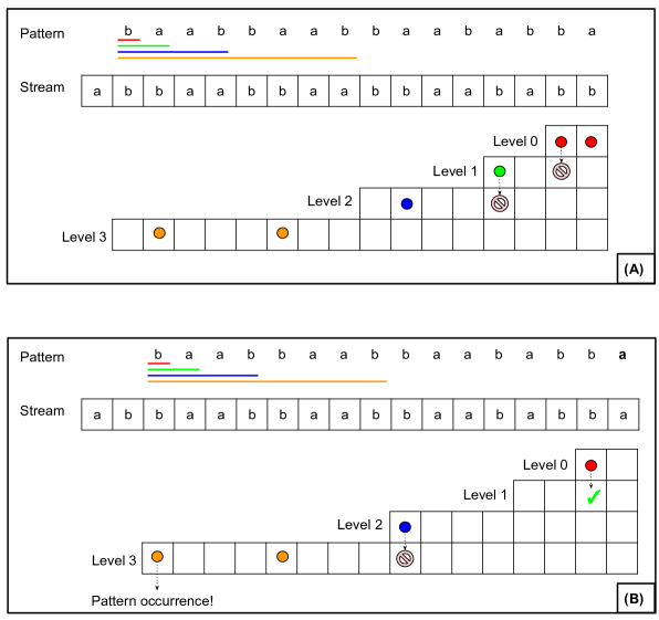
Figure 4.1: Each colored dot at level $i$ represents an occurrence of a prefix of length $2^{i}$ of the pattern (underlined with corresponding color). (A) We have two such occurrences at level 0, one occurrence at levels 1 and 2, and two occurrences at level 3. Some of these occurrences are candidates that could be promoted to the next level: these are the leftmost occurrences at levels 0 and 1. Unfortunately, none of these occurrences can be promoted since they are not occurrences of a prefix of length $2^{i+1}$ of the pattern: the leftmost occurrence at level 0 is not an occurrence of ”ba” and the occurrence at level 1 is not an occurrence of ”baab”. They will therefore be eliminated before the next stream’s character arrives. (B) A new stream character (”a”, in bold) has arrived. All occurrences, except the eliminated ones, have been shifted to the left in the levels’ windows. Now, three occurrences are candidates that could be promoted to the next level. The occurrence at level 0 is indeed an occurrence of ”ba”, therefore it will be promoted to level 1 before the next stream’s character arrives. The occurrence at level 2 is not an occurrence of ”baabbaab”, therefore it will be eliminated. Finally, the leftmost occurrence at level 3 is an occurrence of the full pattern: before removing it from the window, we will increment the counter $occ$ and report this new occurrence.

Compressing the occurrences

We have $\log n$ levels, however this is not sufficient to claim that the algorithm uses $O(\log n)$ space: in each level $i$, there could be up to $2^{i}$ occurrences of the pattern’s prefix $y[1,2^{i}]$. In this paragraph we show that all the occurrences in a window can be compressed in just $O(1)$ words of space.

The key observation is that, in each level, we store occurrences of the pattern’s prefix of length $K=2^{i}$ in a window of size $2K=2^{i+1}$. Now, if there are at least three such occurrences, then at least two of them must overlap. But these are occurrences of the same string $y[1,2^{i}]$, so if they overlap the string must be periodic. Finally, if the string is periodic then all its occurrences in the window must be equally-spaced: we have an occurrence every $p$ positions, for some integer $p$ (a period of the string). Then, all $t$ occurrences $W_{i}=\{r_{1},r_{2},\dots,r_{t}\}$ in the window can be encoded in just $O(1)$ space by storing the first occurrence $r_{1}$, the number $t$ of occurrences, and the period $p$. This representation is also easy to update (in constant time) upon insertion of new occurrences to the right (which must follow the same rule) and removal of an occurrence to the left. We now formalize this reasoning.

Definition 4.1.3 (Period of a string).

Let $S$ be a string of length $K$. We say that $S$ has period $p$ if and only if $S[i]=S[i+p]$ for all $1\leq p\leq K-p$.

Example 4.1.4.

The string $S=abcabcabcabca$, of length $K=13$, has periods 3, 6, 9, 12.

Theorem 4.1.5 (Wilf’s theorem).

Any string having periods $p$, $q$ and length at least $p+q-gcd(p,q)$ also has $gcd(p,q)$ as a period.

Example 4.1.6.

Consider the string above: $S=abcabcabcabca$. The string has periods $6$, $9$ (with $gcd(6,9)=3$) and has length $13>6+9-3=12$. Wilf’s theorem can be used to deduce that the string must also have period $gcd(6,9)=3$.

Wilf’s theorem can be used to prove the following (exercise):

Lemma 4.1.7.

Let $P$ be a string of length $K$, and $S$ be a string of length $2K$. If $P$ occurs in $S$ at positions $r_{1}<r_{2}<\dots<r_{t}$, with $t\geq 3$, then $r_{j+1}=r_{j}+p$, where $p=r_{2}-r_{1}$.

The lemma provides a compressed representation for all the occurrences $W_{i}=\{r_{1},r_{2},\dots,r_{t}\}$ in the window at each level $i$: just record $(r_{1},t,p)$. This representation is easy to update in constant time when $r_{1}$ is removed from $W_{i}$ and when a new occurrence $r_{t+1}$ (greater than $r_{t}$) is inserted into $W_{i}$ (these are the only two updates we perform on the sets $W_{i}$).

Updating the fingerprints

The last thing to show is how to efficiently compute $w_{i}=\kappa_{q,z}(x[j-2^{i+1},j-1])$ at level $i$ (needed at Line 1 of the algorithm), that is, the fingerprint of the whole window when the first occurrence stands at the beginning of the window: $r_{1}=j-2^{i+1}$. Consider the window $W_{i}$ at level $i$, and the two smallest positions $r_{1},r_{2}\in W_{i}$. Let $x=x[1,j-1]$ be the current stream. We keep in memory three fingerprints (see Figure 4.2):

1. $\kappa_{q,z}(x)$: the fingerprint of the whole stream.

2. $\kappa_{q,z}(x[r_{1},r_{2}-1])$: the fingerprint of the stream’s substring standing between $r_{1}$ (included) and $r_{2}$ (excluded), whenever $W_{i}$ contains at least two positions.

3. $\kappa_{q,z}(x[1,r_{1}-1])$: the fingerprint of the stream’s prefix ending at $r_{1}-1$, whenever $W_{i}$ contains at least one position.

Figure 4.2: For each level (window), we keep three fingerprints: A (full stream, unique for all windows), B (string between first two pattern’s occurrences), and C (from beginning of the stream to the first pattern’s occurrence).

Knowing A,B, and C we can easily compute the fingerprint $w_{i}$ of the whole window when $r_{1}=j-2^{i+1}$:

$$w_{i}=A-C\cdot z^{2^{i+1}}\mod q$$

Note that $z^{2^{i+1}}\mod q$ can easily be pre-computed for any $i\leq\log n$ at the beginning of the algorithm using the recurrence $z^{2^{i+1}}=(z^{2^{i}})^{2}$. We now show how to update the three fingerprints A, B, C.

Updating A

Fingerprint A - the full stream - can be updated very easily in constant time each time a new stream character arrives (see Section 3.1).

Updating B - case 1

B needs to be updated in two cases. The first case happens when $r_{2}$ enters in the window (before that, only $r_{1}$ was in the window): see Figure 4.3. Then, notice that $x[r_{2},j-1]=y[1,2^{i}]$, so we have the fingerprint $D=\kappa_{q,z}(y[1,2^{i}])=\kappa_{q,z}(x[r_{2},j-1])$.

Figure 4.3: Updating B - case 1: $r_{2}$ enters in the window.

It follows that B can be computed as:

$$B=\left(A-D-C\cdot z^{|D|+|B|}\right)\cdot z^{-|D|}\mod q$$

In the above equation, the quantity $z^{|D|+|B|}\equiv_{q}z^{2^{i}+(r_{2}-r_{1})}$ can be computed one step at a time (i.e. multiplying $z$ by itself $2^{i}+(r_{2}-r_{1})$ times modulo $q$) while the stream characters between $r_{1}$ and $r_{2}+2^{i}-1$ arrive (constant time per character per level). The $\log n$ values $z^{-|D|}=z^{-2^{i}}\mod q$ can be pre-computed before the stream arrives in $O(\log m)$ time as follows. $z^{2^{i+1}}\equiv_{q}(z^{2^{i}})^{2}$, and $z^{-2^{i}}\mod q$ can be computed in $O(\log q)=O(\log m)$ time using the equality $a^{-1}\equiv_{q}a^{q-2}$ and fast exponentiation: $z^{-2^{i}}\equiv_{q}z^{2^{i}\cdot(q-2)}$.

Updating B - case 2

The second case where we need to update B is when $r_{1}$ exits the window and $r_{3}$ is in the window: $B$ should become the fingerprint of the string between $r_{2}$ and $r_{3}$. See Figure 4.4.

Figure 4.4: Updating B - case 2: $r_{1}$ exits the window and $r_{3}$ is in the window.

It turns out that in this case nothing needs to be done: The new fingerprint is $B^{\prime}=B$. To see this, note that (1) $r_{3}-r_{2}=r_{2}-r_{1}$ by Lemma 4.1.7, and (2) $r_{1}$ and $r_{2}$ are both occurrences of the same string of length $2^{i}$. Since $r_{2}-r_{1}\leq 2^{i}$, then $x[r_{1},r_{2}-1]=x[r_{2},r_{3}-1]$.

Updating C - case 1

C needs to be updated in two cases. The first case happens when $r_{1}$ enters in the window (before that, the window was empty: $W_{i}=\emptyset$). See Figure 4.5. As in case B1, notice that we have the fingerprint $D=\kappa_{q,z}(y[1,2^{i}])=\kappa_{q,z}(x[r_{1},j-1])$.

Figure 4.5: Updating C - case 1: $r_{1}$ enters in the window.

Then:

$$C=(A-D)\cdot z^{-|D|}\mod q$$

Updating C - case 2

The last case to consider is when $r_{1}$ exits the window and $r_{2}$ is in the window. See Figure 4.6.

Figure 4.6: Updating C - case 2: $r_{1}$ exits the window and $r_{2}$ is in the window.

This is achieved as follows:

$$C^{\prime}=C\cdot z^{|B|}+B\mod q$$

where $z^{|B|}\equiv_{q}z^{r_{2}-r_{1}}$ is computed as $z^{r_{2}-r_{1}}\equiv_{q}z^{2^{i}+(r_{2}-r_{1})}\cdot z^{-2^{i}}$ (both computed as in case B).

Final result

Observe that each fingerprint update can be performed in constant time (per level, thus $O(\log n)$ time per stream’s character). We obtain:

Theorem 4.1.8.

Let $m$ be the stream’s length and $n\leq m$ be the pattern’s length. Porat-Porat’s algorithm solves the pattern matching problem in the streaming model using $O(\log n)$ words of memory and $O(\log n)$ delay. The correct solution is returned with high (inverse-polynomial) probability $1-m^{-c}$, for any constant $c\geq 1$ chosen at initialization time.

Breslauer and Galil in [3] reduced the delay to $O(1)$ while still using $O(\log n)$ words of space.

4.1.3 Extension to approximate pattern matching

We describe a modification of Porat-Porat’s algorithm that allows finding all stream occurrences $x_{i,n}=x_{i}\dots x_{i+n-1}$ of a pattern $y=y_{1}\dots y_{n}$ such that $d_{H}(x_{i,n},y)\leq k$ for any parameter $k$, where $d_{H}$ is the Hamming distance between strings.

For simplicity, we first describe the algorithm for $k=1$, i.e. zero or one mismatch between the pattern and the stream. Let $y_{i:d}=y_{i}\ y_{i+d}\ y_{i+2d}\dots$. In other words, $y_{i:d}$ is the sub-pattern built by extracting one every $d$ characters from $y$, starting from character $y_{i}$. We call $y_{i:d}$ a shift of $y$.

Consider two strings $x$ and $y$, both of the same length $n$. Clearly, $x=y$ if and only if $x_{i:d}=y_{i:d}$ for all $i=1,\dots,d$. Assume now that $d_{H}(x,y)=1$. Then, note that the error is captured by exactly one of the $d$ shifts: there exists one $i^{\prime}\in[1,d]$ such that $x_{i^{\prime}:d}\neq y_{i^{\prime}:d}$, and $x_{i:d}=y_{i:d}$ for all $i\neq i^{\prime}$.

Example 4.1.9.

Let $x=$abracadabra and $y=$abbacadabra, with $d_{H}(x,y)=1$ (the mismatch is underlined). Pick $d=2$ and consider the two shifts (per word) $x_{1:2}=$ arcdba, $x_{2:2}=$baaar, $y_{1:2}=$ abcdba, $y_{2:2}=$baaar. Then:

• $x_{1:2}\neq y_{1:2}$

• $x_{2:2}=y_{2:2}$

What if $d_{H}(x,y)=k>1$? Then, the number of shifts $i^{\prime}$ such that $x_{i^{\prime}:d}\neq y_{i^{\prime}:d}$ could be smaller than $k$ (but never larger). Notice that this happens precisely when the distance $|j^{\prime}-j|$ between two mismatches $x_{j}\neq y_{j}$ and $x_{j^{\prime}}\neq y_{j^{\prime}}$ is a multiple of $d$.

Example 4.1.10.

Let $x=$abracadabra and $y=$abbacaaabra, with $d_{H}(x,y)=2$ (the two mismatches are underlined). Pick $d=2$ and consider the two shifts (per word) $x_{1:2}=$ arcdba, $x_{2:2}=$baaar, $y_{1:2}=$ abcaba, $y_{2:2}=$baaar. Then:

• $x_{1:2}\neq y_{1:2}$

• $x_{2:2}=y_{2:2}$

In particular, the Hamming distance is 2 but only one of the two shifts generates a mismatch. This happens because the two mismatches are distanced 4 positions, which is a multiple of $d=2$.

It is easy to see that the above issue does not happen if $d$ does not divide the distance between the two mismatches.

Example 4.1.11.

Let $x=$abracadabra and $y=$abbacaaabra, with $d_{H}(x,y)=2$ (the two mismatches are underlined). Pick $d=3$ and consider the three shifts (per word) $x_{1:3}=$aadr, $x_{2:3}=$bcaa, $x_{3:3}=$rab, $y_{1:3}=$aaar, $y_{2:3}=$bcaa, $y_{3:3}=$bab. Then:

• $x_{1:3}\neq y_{1:3}$

• $x_{2:3}=y_{2:3}$

• $x_{3:3}\neq y_{3:3}$

Now, two shifts generates a mismatch.

This property can be summarized in a corollary:

Corollary 4.1.11.1.

Let $x,y$ be two words of length $n$, and consider their $d$ shifts $x_{i:d},y_{i:d}$ for $i=1,\dots,d$. Then:

• If $d_{H}(x,y)=0$, then $x_{i:d}=y_{i:d}$ for all $i=1,\dots,d$.

• If $d_{H}(x,y)=1$, then $x_{i:d}\neq y_{i:d}$ for exactly one $i\in[1,d]$.

• If $d_{H}(x,y)>1$, then $x_{i:d}\neq y_{i:d}$ for at least two values $i\in[1,d]$, provided that there exist two mismatches whose distance $|j-j^{\prime}|$ is not a multiple of $d$.

Consider the distance $|j-j^{\prime}|$ between (the positions of) any two mismatches between $x$ and $y$. Consider moreover the smallest $\lceil\log_{2}n\rceil$ prime numbers $P=\{p_{1},p_{2},\dots,p_{\lceil\log_{2}n\rceil}\}$. Clearly, $|j-j^{\prime}|$ cannot be a multiple of all numbers in $P$: this would imply that $|j-j^{\prime}|\geq\prod_{p\in P}p>n$. This immediately suggests an algorithm for pattern matching at Hamming distance at most 1 between two strings $x,y$ of length $n$:

1. For each $d\in P=\{p_{1},p_{2},\dots,p_{\lceil\log_{2}n\rceil}\}$, do the following:

2. For each $i=1,\dots,d$, compare $x_{i:d}$ and $y_{i:d}$. If at least two values of $i\in[1,d]$ are such that $x_{i:d}\neq y_{i:d}$, then exit and output “$d_{H}(x,y)>1$”.

3. If step (2) never exits, then output “$d_{H}(x,y)\leq 1$”.

It is straightforward to adapt the above algorithm to the case where $x$ is streamed and $|x|=m>n$: just break the stream into $d$ sub-streams (i.e. $x_{i}\ x_{i+d}\ x_{i+2d}\dots$, for all $i=1,\dots,d$), for every $d\in P$. This allows implementing the comparisons $x_{i:d}\stackrel{{\scriptstyle?}}{{=}}y_{i:d}$ using Porat-Porat’s algorithm. Note that we run $O(\log^{2}n)$ parallel instances of Porat-Porat’s algorithm. We obtain:

Theorem 4.1.12.

Let $m$ be the stream’s length and $n\leq m$ be the pattern’s length. The above modification of Porat-Porat’s algorithm finds all occurrences of the pattern at Hamming distance at most 1 in the stream using $O(\log^{3}n)$ words of memory and $O(\log^{3}n)$ delay. The correct solution is returned with high probability.

We can easily extend the above idea to $k\geq 1$ mismatches. Assume that $d_{H}(x,y)>k$. Consider any group of $k+1$ mismatches between $x$ and $y$, at positions $i_{1}<\dots<i_{k+1}$. We want to find a prime number $d\geq k+1$ such that $d$ does not divide $i_{j}-i_{j^{\prime}}$, for all $1\leq j^{\prime}<j\leq k+1$. Then, we are guaranteed that $x_{i:d}\neq y_{i:d}$ for at least $k+1$ shifts $i$, since no pair of mismatches $i_{j},i_{j^{\prime}}$ can fall in the same shift (which would imply that $d$ divides $|i_{j}-i_{j^{\prime}}|$). Note: we require that $d$ is greater than or equal to $k+1$ because the number of shifts is $d$ and we need at least $k+1$ distinct mismatching shifts of $x$ and $y$ in order to detect Hamming distance $>k$.

The integer $d$ does not divide $i_{j}-i_{j^{\prime}}$ for all $1\leq j^{\prime}<j\leq k+1$ if and only if $d$ does not divide their product $\prod_{1\leq j^{\prime}<j\leq k+1}(i_{j}-i_{j^{\prime}})\leq n^{(k+1)^{2}}$. We will surely find such an integer $d$ in the set $P$ of the smallest $\log_{2}n^{(k+1)^{2}}=O(k^{2}\log n)$ prime numbers greater than or equal to $k+1$ (actually, we could slightly improve this analysis: since each prime is larger than or equal to $k$, the number of such primes is at most $\log_{k}n^{(k+1)^{2}}=O(\frac{k^{2}\log n}{\log k})$). The pattern matching algorithm works exactly as in the case $k=1$, except that we now look for a prime $d\in P$ such that $x_{i:d}\neq y_{i:d}$ for at least $k+1$ values of $i\in[1,d]$. We obtain (the notation $\tilde{O}(\cdot)$ hides $\mathrm{polylog}(n)$ multiplicative factors):

Theorem 4.1.13.

The above modification of Porat-Porat’s algorithm finds all occurrences of the pattern at Hamming distance at most $k$ in the stream using $\tilde{O}(k^{4})$ words of memory and $\tilde{O}(k^{4})$ delay. The correct solution is returned with high probability.

In their original article [26], Porat and Porat describe a more efficient solution of $\tilde{O}(k^{3})$ space and $\tilde{O}(k^{2})$ delay. Clifford et al. in [6] improved this to $\tilde{O}(\sqrt{k})$ delay and $\tilde{O}(k^{2})$ space. These bounds were further improved in [7] to $\tilde{O}(\sqrt{k})$ delay and $\tilde{O}(k)$ space. The authors of [7] prove that these latter bounds are optimal (up to poly-logarithmic factors).

4.2 Probabilistic counting

Consider the basic task of counting. In order to count up to $m$ we clearly need $\log m$ bits (logarithms are base 2). What if we allow for a 2-approximation, that is, we allow our register to be off by at most a factor of two? then, it is easy to see that $\log\log m$ bits are sufficient: instead of storing our number $x<m$, we store the largest power of two not exceeding it: $2^{y}\leq x$, with $y=\lfloor\log x\rfloor$. Since $y$ takes integer values between $0$ and $\log m$, it only takes at most $\log\log m$ bits to store it. In general, we may fix a relative error $0<\epsilon\leq 1$ and approximate $x$ with the largest power of $(1+\epsilon)$ not exceeding it: $(1+\epsilon)^{y}\leq x$, with $y=\lfloor\log_{1+\epsilon}x\rfloor=\left\lfloor\frac{\log x}{\log(1+\epsilon)}\right\rfloor$. Then, $y$ requires just $\log\log m-\log\log(1+\epsilon)\leq\log\log m+O(\log(\epsilon^{-1}))$ bits to be stored (logarithms are base 2 unless otherwise specified; we used the bound $\log(1+\epsilon)\geq\frac{1}{1/\epsilon+1/2}$ and assumed $0<\epsilon<1$) and is a $\epsilon$-approximation of $x$.

Example 4.2.1.

Suppose we allow for a $10\%$ relative error (i.e. $\epsilon=0.1$). Then, we need approximately just $\log\log m+3$ bits. What is the largest number we can store in 8 bits? Solving $\log\log m+3=8$ we obtain $\log\log m=5$, i.e. we can store a number as large as $2^{2^{5}}=2^{32}$ with 10% relative error.

While the above reasoning shows how one can store approximately a large counter in a small number of bits, it does not show how to increment such counter: in real-case applications, we may wish to start from an approximate counter initialized with 0 and increase it one unit at a time (for example, every time a certain event occurs). In the next section we see that this goal can be achieved by using randomization, incrementing the counter with some small probability.

4.2.1 Morris’ algorithm

In 1978 Robert Morris, a computer scientist working at Bell labs, faced the problem of counting large numbers using very small (8 bits) registers. Using just 8 bits, the largest number that can be stored (without skipping any positive integer) is clearly 255. However, as seen above, this is true only if we wish to store exact counts; if we allow for some error, then the register can actually hold larger numbers. Algorithm 2 shows the basic algorithm devised by Morris, first described in [23]. The algorithm uses just one register ($X$) and its failure probability $1/(2\epsilon^{2})$ makes it useful only for $\epsilon>1/\sqrt{2}$, since otherwise the bound on the failure probability $1/(2\epsilon^{2})$ is larger than one (thus not meaningful). In the next sections we will initialize several parallel versions of the algorithm to further boost the success probability.

input : A stream of $m$ events and a desired relative error $0<\epsilon\leq 1$

output : A $(1\pm\epsilon)$-approximation $\hat{m}$ of the number $m$ of events in the stream, with failure probability $1/(2\epsilon^{2})$

1

2Initialize a register $X=0$;

3 For each event to be counted: increment $X$ with probability $2^{-X}$;

4 Finally, output $2^{X}-1$;

5

Algorithm 2 Morris

4.2.2 Analysis

This analysis of the algorithm has been adapted from [16, 25, 15]. We first prove that the estimator $2^{X}-1$ returned by the algorithm is unbiased:

Lemma 4.2.2.

$E[2^{X}-1]=m$

Proof.

We proceed by induction on $m$. Let us denote with $X_{i}$ the register’s content after event $i$. For $m=0$, we have $X_{0}=0$ and $E[2^{X_{0}}-1]=0$ so we are done. Assume inductively that the claim holds for $m$, i.e. $E[2^{X_{m}}-1]=m$ (equivalently, $E[2^{X_{m}}]=m+1$). Then, applying the law of total expectation to the partition $\{X_{m}=i\}$ of the event space we have:

$$\begin{array}[]{ccl}E[2^{X_{m+1}}-1]&=&E[2^{X_{m+1}}]-1\\ &=&\left(\sum_{i=0}^{\infty}P(X_{m}=i)\cdot E[2^{X_{m+1}}\ |\ X_{m}=i]\right)-1\\ \end{array}$$

Observe that

$$\begin{array}[]{ccl}E[2^{X_{m+1}}\ |\ X_{m}=i]&=&P(X_{m}=i\mathrm{\ is\ incremented})\cdot 2^{i+1}+\\ &&P(X_{m}=i\mathrm{\ is\ not\ incremented})\cdot 2^{i}\\ &=&2^{-i}\cdot 2^{i+1}+(1-2^{-i})\cdot 2^{i}\\ &=&2^{i}+1\end{array}$$

so:

$$\begin{array}[]{ccl}E[2^{X_{m+1}}-1]&=&\left(\sum_{i=0}^{\infty}P(X_{m}=i)\cdot(2^{i}+1)\right)-1\\ &=&\left(\sum_{i=0}^{\infty}P(X_{m}=i)\cdot 2^{i}+\sum_{i=0}^{\infty}P(X_{m}=i)\right)-1\\ &=&\sum_{i=0}^{\infty}P(X_{m}=i)\cdot 2^{i}\\ &=&E[2^{X_{m}}]=m+1\\ \end{array}$$

∎

Having established that the expected value of our estimator is exactly the count $m$ that we wish to store, we only miss to establish how much a single realization of the estimator can differ from the expected value. We first compute the estimator’s variance:

Lemma 4.2.3.

$Var[2^{X}-1]\leq m^{2}/2$

Proof.

$$\begin{array}[]{ccl}Var[2^{X}-1]&=&E[((2^{X}-1)-m)^{2}]\\ &=&E[(2^{X}-(m+1))^{2}]\\ &=&E[2^{2X}]-2(m+1)E[2^{X}]+(m+1)^{2}\\ &=&E[2^{2X}]-(m+1)^{2}\\ \end{array}$$ (4.1)

Let $X_{m}$ denote the value of our register after seeing $m$ events. We now compute $E[2^{2X_{m}}]$ and plug it into Equation 4.1.

$$\begin{array}[]{ccl}E[2^{2X_{m}}]&=&\sum_{i=0}^{\infty}P(X_{m}=i)\cdot 2^{2i}\\ &=&\sum_{i=0}^{\infty}2^{2i}\cdot\left(P(X_{m-1}=i-1)\cdot 2^{-(i-1)}+P(X_{m-1}=i)\cdot(1-2^{-i})\right)\\ &=&\sum_{i=0}^{\infty}2^{i+1}\cdot P(X_{m-1}=i-1)+\sum_{i=0}^{\infty}2^{2i}\cdot P(X_{m-1}=i)-\sum_{i=0}^{\infty}2^{i}\cdot P(X_{m-1}=i)\\ &=&\sum_{i=0}^{\infty}4\cdot 2^{i-1}\cdot P(X_{m-1}=i-1)+\sum_{i=0}^{\infty}2^{2i}\cdot P(X_{m-1}=i)-\sum_{i=0}^{\infty}2^{i}\cdot P(X_{m-1}=i)\\ &=&4\cdot E[2^{X_{m-1}}]+E[2^{2X_{m-1}}]-E[2^{X_{m-1}}]\\ &=&3\cdot E[2^{X_{m-1}}]+E[2^{2X_{m-1}}]\\ &=&3m+E[2^{2X_{m-1}}]\\ \end{array}$$

The above yields a recursive definition: denoting $E_{m}=E[2^{2X_{m}}]$, we have $E_{m}=3m+E_{m-1}$. Since $E_{0}=E[2^{2\cdot 0}]=1$, this series expands to $E_{m}=\sum_{i=1}^{m}3i+1=\frac{3m(m+1)}{2}+1$. We can finally plug this into Equation 4.1 and obtain

$$\begin{array}[]{ccl}Var[2^{X}-1]&=&E[2^{2X}]-(m+1)^{2}\\ &=&\frac{3m(m+1)}{2}+1-(m+1)^{2}\\ &=&(m^{2}-m)/2\leq m^{2}/2\\ \end{array}$$

∎

We have established that the variance is at most $m^{2}/2$, thus our estimator on average differs by $\sqrt{m^{2}/2}=m/\sqrt{2}$ (standard deviation) from the expected value $m$. Applying Chebyshev we get our first bound on the relative error. For any $0<\epsilon<1$:

$$P(|(2^{X}-1)-m|\geq m\cdot\epsilon)\leq\frac{Var[2^{X}-1]}{m^{2}\epsilon^{2}}\leq\frac{1}{2\epsilon^{2}}$$

Note that for $\epsilon<1/\sqrt{2}$ the probability on the right-hand side is greater than 1 and the bound is not informative. For this reason, we cannot directly apply a Chernoff-Hoeffding result: it would only work for $\epsilon>1/\sqrt{2}$. Before applying Chernoff-Hoeffding, we will therefore boost this probability and make it constant (using boosted Chebyshev).

4.2.3 A first improvement: Morris+

A first improvement, indicated here with the name Morris+, can be achieved by simply applying Lemma 1.2.3 (boosted Chebyshev) to the results of $s=\frac{3}{2\epsilon^{2}}=O(1/\epsilon^{2})$ independent (parallel) instances of the algorithm. Let us denote with $\Theta^{+}$ the mean of the $s$ results. Then, Lemma 1.2.3 yields:

$$P(|\Theta^{+}-m|>m\cdot\epsilon)\leq\frac{1}{s\cdot 2\epsilon^{2}}\leq\frac{1}{3}$$

This bound is clearly better than the previous one: we fail with constant probability $1/3$, no matter the desired relative error. Note that the price to pay is a higher space usage: now we need to keep $s=O(1/\epsilon^{2})$ independent registers. Note also that the error could be made arbitrarily small by increasing $s$: the space increases linearly with $s$, and the failure probability decreases linearly with $s$. In the next paragraph we show how to achieve an exponentially-decreasing failure probability with one final (standard) trick: taking the median of independent instances of Morris+.

4.2.4 Final algorithm: Morris++

The final step is to execute $t$ independent parallel instances of Morris+. Note that each of the $t$ instances consists of $s$ parallel instances of (the basic) Morris’ algorithm, so in the end we will have $st$ parallel instances (each with its own independent register). Let us denote with $\Theta^{+}_{1},\dots,\Theta^{+}_{t}$ the $t$ instances of Morris+. The output of our algorithm Morris++ is the median $\Theta^{++}=\mathrm{median}\{\Theta^{+}_{1},\dots,\Theta^{+}_{t}\}$ of the $t$ instances. We now show that the median is indeed correct (has relative error bounded by $\epsilon$) with high probability, and we compute the total space usage (i.e. number of register) required in order to guarantee relative error $\epsilon$ with probability at least $1-\delta$, for any choice of $\epsilon$ and $\delta$. We state the result as a general Lemma, since it will be useful also in other results.

Lemma 4.2.4.

Let $\Theta^{+}$ be an estimator such that $E[\Theta^{+}]=m$ and $P(|\Theta^{+}-m|>m\cdot\epsilon)\leq\frac{1}{3}$. For any desired failure probability $\delta$, draw $t=72\ln(1/\delta)$ instances of the estimator and define $\Theta^{++}=\mathrm{median}\{\Theta^{+}_{1},\dots,\Theta^{+}_{t}\}$. Then:

$$P(|\Theta^{++}-m|>m\cdot\epsilon)\leq\delta$$

Proof.

Consider the following indicator random variable:

$$\mathbbm{1}_{i}=\left\{\begin{array}[]{cl}1&\mathrm{if\ |\Theta^{+}_{i}-m|\geq m\cdot\epsilon}\\ 0&\mathrm{otherwise}\end{array}\right.$$

That is, $\mathbbm{1}_{i}$ is equal to 1 if and only if $\Theta^{+}_{i}$ fails, i.e. if its relative error exceeds $\epsilon$. From the previous subsection, note that $\mathbbm{1}_{i}$ takes value 1 with probability at most $1/3$.

What is the probability that $\Theta^{++}$ fails, i.e. that $|\Theta^{++}-m|\geq\epsilon\cdot m$? If the median fails, then it is either too small (below $(1-\epsilon)\cdot m$) or too large (above $(1+\epsilon)\cdot m$). In either case, by definition of median, at least $t/2$ estimators $\Theta^{+}_{i}$ return a result which is too small or too large, and thus fail. In other words,

$$P(|\Theta^{++}-m|\geq\epsilon\cdot m)\leq P\left(\sum_{i=1}^{t}\mathbbm{1}_{i}\geq t/2\right)$$

As seen above, each $\mathbbm{1}_{i}$ is a Bernoullian R.V. taking value 1 with probability at most $1/3$. We thus have $\mu=E[\sum_{i=1}^{t}\mathbbm{1}_{i}]\leq t/3$. Clearly, decreasing $\mu$ decreases also the probability that $\sum_{i=1}^{t}\mathbbm{1}_{i}$ exceeds $t/2$ (see also the following Chernoff-Hoeffding bound), so for simplicity in the following calculations we will consider $\mu=t/3$ (we aim at an upper-bound to this probability so this simplification is safe).

Recall the one-sided right variant of the Chernoff-Hoeffding additive bound (Lemma 1.2.4):

$$P\left(\sum_{i=1}^{t}\mathbbm{1}_{i}\geq\mu+k\right)=P\left(\sum_{i=1}^{t}\mathbbm{1}_{i}\geq\frac{t}{3}+k\right)\leq e^{\frac{-k^{2}}{2t}}$$

Solving $t/3+k=t/2$, we obtain $k=t/6$. Replacing this value into the previous inequality, we obtain:

$$P\left(\sum_{i=1}^{t}\mathbbm{1}_{i}\geq t/2\right)\leq e^{-t/72}$$

We want the probability on the right-hand side to equal our parameter $\delta$. Solving $\delta=e^{-t/72}$ we obtain $t=72\ln(1/\delta)$. ∎

Since we previously established that Morris+ uses $s=3/(2\epsilon^{2})$ registers, in total Morris++ uses $st=O(\epsilon^{-2}\ln(1/\delta))$ registers. The last thing to notice is that each register stores a number ($X_{m}$) whose expected value is $\log m$, so each register requires on expectation $\log\log m$ bits. We can state our final result:

Theorem 4.2.5.

For any desired relative error $0<\epsilon\leq 1$ and failure probability $0<\delta<1$, the algorithm Morris++ uses $O\left(\frac{\log(1/\delta)}{\epsilon^{2}}\log\log m\right)$ bits on expectation and, with probability at least $1-\delta$, counts numbers up to $m$ with relative error at most $\epsilon$, i.e. it returns a value $\Theta^{++}$ such that:

$$P(|\Theta^{++}-m|>m\cdot\epsilon)\leq\delta$$

4.3 Counting distinct elements

In this section we consider the following problem. Suppose we observe a stream of $m$ integers $x_{1},x_{2},x_{3},\dots,x_{m}$ (arriving one at a time) from the interval $x_{i}\in[1,n]$ and we want to count the number of distinct integers in the stream, i.e. $d=|\{x_{1},x_{2},\dots,x_{m}\}|$. We cannot afford to use too much memory (and $m$ and $d$ are very large — typically in the order of billions).

Here are reported some illuminating examples of the practical relevance of the count-distinct problem. Some of these examples are taken from the paper [12].

Example 4.3.1 (DoS attacks).

Denial of Service attacks can be detected by analyzing the number of distinct flows (source-destination IP pairs contained in the headers of TCP/IP packets) passing through a network hub in a specific time interval. The reason is that typical DoS software use large numbers of fake IP sources; if they were to use few IP sources, then those sources could be easily identified (and blocked) because of the large traffic they must generate in order for the DoS attack to be effective.

Example 4.3.2 (Spreading rate of a worm).

Worms are self-replicating malware whose goal is to spread to as many computers as possible using a network (e.g. the Internet) as medium. In order to count how many computers have been infected by the worm, one needs to (1) filter packets containing the worm’s code, and (2) count the number of distinct source IPs in the headers of those packets. From https://www.caida.org/archive/code-red/ (an analysis of the spread of the Code-Red version 2 worm between midnight UTC July 19, 2001 and midnight UTC July 20, 2001):

”On July 19, 2001 more than 359,000 computers were infected with the Code-Red (CRv2) worm in less than 14 hours. At the peak of the infection frenzy, more than 2,000 new hosts were infected each minute.”

Example 4.3.3 (Distinct IPs/post views).

Suppose we wish to count how many people are visiting our web site. Then, we need to count how many distinct IP numbers are connecting to the server that hosts the web site. The same problem occurs with post views; in this case, the problem is more serious since the problem must be solved for each post! Reddit uses a randomized cardinality estimation algorithm (HLL) to count post views: https://www.redditinc.com/blog/view-counting-at-reddit/.

4.3.1 Naive solutions

A first naive solution to the count-distinct problem is to keep a bitvector $B[1,n]$ of $n$ bits, initialized with all 0’s. Then it is sufficient to set $B[x_{i}]=1$ for each element $x_{i}$ of the stream. Finally, we count the number of 1’s in the bitvector. If $n$ is very large (like in typical applications), this solution uses too much space. A second solution could be to store the stream elements in a self-balancing binary search tree or in a hash table with dynamic re-allocation. This solution uses $O(d\log n)$ bits of space, which could still be too much if the number $d$ of distinct elements is very large. In the next sections we will see how to compute an approximate answer within logarithmic space. We first discuss an idealized algorithm, which however assumes a uniform hash function and thus cannot actually be implemented in small space. Then, we study a practical variant (bottom-k) which only requires pairwise-independent hash functions and can thus be implemented in truly logarithmic space.

4.3.2 Idealized Flajolet-Martin’s algorithm

The following solution is an idealized version (requiring totally uniform hash functions) of the algorithm described by Flajolet and Martin in [14]. Let $[1,n]$ denote the range of integers $1,2,\dots,n$ and $[0,1]$ denote the range of all real values between 0 and 1, included. We use a uniform hash function $h:[1,n]\rightarrow[0,1]$. Note that such a function actually requires $\Theta(n)$ words of space to be stored, see Section 1.3: the algorithm is not practical, but we describe it for its simplicity.

input : A stream of integers $x_{1},\dots,x_{m}$.

output : An estimate $\hat{d}$ of the number of distinct integers in the stream.

1

2Initialize $y=1$;

3 For each stream element $x$, update $y\leftarrow\min(y,h(x))$;

4 When the stream ends, return the estimate $\hat{d}=\frac{1}{y}-1$;

5

Algorithm 3 FM

Intuitively, why does FM work? First, note that repeated occurrences of some integer $x$ in the stream will yield the same hash value $h(x)$. Since $h$ is uniform, we end up drawing $d$ uniform real numbers $y_{1}<y_{2}<\dots<y_{d}$ in the interval $[0,1]$ . At the end, the algorithm returns $1/y_{1}-1$. The more distinct $y_{i}$’s we see, the more likely it is to see a smaller value. In particular, $h$ will spread the $y_{i}$’s uniformly in the interval $[0,1]$; think, for a moment, about the most ”uniform” (regular) way to spread those numbers in $[0,1]$: this happens when the intervals $[0,y_{1}]$, $[y_{i},y_{i+1}]$, $[y_{d},1]$ have all the same length $y_{i+1}-y_{i}=y_{1}-0=y_{1}=1/(d+1)$. But then, our claim $1/y_{1}-1=d$ follows. It turns out that this is true also on average (not just in this idealized ”regular” case): the average distance between $0$ and the smallest hash $y_{1}$ seen in the stream is precisely $1/(d+1)$. Next, we prove this intuition.

Lemma 4.3.4.

Let $y=\min\{h(x_{1}),\dots,h(x_{m})\}$. Then, $E[y]=1/(d+1)$.

Proof.

$$\begin{array}[]{rcll}E[y]&=&\int_{0}^{1}P(y\geq\lambda)\,d\lambda&\hskip 28.45274pt\mathrm{Lemma\ \ref{lem:expected CDF}}\\ &=&\int_{0}^{1}P(\forall x_{i}\ :\ h(x_{i})\geq\lambda)\,d\lambda&\\ &=&\int_{0}^{1}(1-\lambda)^{d}\,d\lambda&\hskip 28.45274pth\ \mathrm{is\ uniform}\\ &=&-\frac{(1-\lambda)^{d+1}}{d+1}\ \bigg{|}^{1}_{0}&\\ &=&\frac{1}{d+1}&\end{array}$$

∎

Unfortunately, in general $E[1/y]\neq 1/E[y]$ so it is not true that $E[\hat{d}]=E[1/y-1]=d$. Technically, we say that $\hat{d}$ is not an unbiased estimator for $d$. On the other hand, if $y$ is very close to $1/(d+1)$, then intuitively also $\hat{d}$ will be very close to $d$. We will prove this intuition by studying the relative error of $y$ with respect to $1/(d+1)$, and then turn this into a relative error of $\hat{d}$ with respect to $d$.

Lemma 4.3.5.

Let $y=\min\{h(x_{1}),\dots,h(x_{m})\}$. Then, $Var[y]\leq 1/(d+1)^{2}$.

Proof.

We use the equality $Var[y]=E[y^{2}]-E[y]^{2}$. We know that $E[y]^{2}=1/(d+1)^{2}$. We compute $E[y^{2}]$ as follows:

$$\begin{array}[]{rcl}E[y^{2}]&=&\int_{0}^{1}P(y^{2}\geq\lambda)\,d\lambda\\ &=&\int_{0}^{1}P(y\geq\sqrt{\lambda})\,d\lambda\\ &=&\int_{0}^{1}(1-\sqrt{\lambda})^{d}\,d\lambda\\ \end{array}$$

We can solve the latter integral by the substitution $u=1-\sqrt{\lambda}$. We have $\lambda=(1-u)^{2}$ and $\frac{d\lambda}{du}=d(1-u)^{2}/du=-2(1-u)$, so $d\lambda=-2(1-u)\,du$. Also, note that $u=0$ for $\lambda=1$ and $u=1$ for $\lambda=0$ so the integral’s interval switches. By applying the substitution we obtain:

$$\begin{array}[]{rcl}E[y^{2}]&=&\int_{0}^{1}(1-\sqrt{\lambda})^{d}\,d\lambda\\ &=&\int_{1}^{0}-2(1-u)u^{d}\,du\\ &=&-2\left(\int_{1}^{0}u^{d}\,du-\int_{1}^{0}u^{d+1}\,du\right)\\ &=&-2\left(\frac{u^{d+1}}{d+1}\bigg{|}^{0}_{1}-\frac{u^{d+2}}{d+2}\bigg{|}^{0}_{1}\right)\\ &=&-2\left(-\frac{1}{d+1}+\frac{1}{d+2}\right)\\ &=&\frac{2}{d+1}-\frac{2}{d+2}\end{array}$$

To conclude:

$$\begin{array}[]{rcl}Var[y]&=&E[y^{2}]-E[y]^{2}\\ &=&\frac{2}{d+1}-\frac{2}{d+2}-\frac{1}{(d+1)^{2}}\\ &=&\frac{2(d+2)-2(d+1)}{(d+1)(d+2)}-\frac{1}{(d+1)^{2}}\\ &=&\frac{2}{(d+1)(d+2)}-\frac{1}{(d+1)^{2}}\\ &\leq&\frac{2}{(d+1)^{2}}-\frac{1}{(d+1)^{2}}\\ &=&\frac{1}{(d+1)^{2}}\end{array}$$

∎

From here, we proceed as in Section 4.2.1. We define an algorithm FM+ that computes the mean $y^{\prime}=\sum_{i=1}^{s}y_{i}/s$ of $s$ independent parallel instances of FM, for some $s$ to be determined later. Applying Chebyshev (Lemma 1.2.3), we obtain

$$P\left(\bigg{|}y^{\prime}-\frac{1}{d+1}\bigg{|}>\frac{\epsilon}{d+1}\right)\leq\frac{1}{(d+1)^{2}}\cdot\frac{(d+1)^{2}}{s\epsilon^{2}}=\frac{1}{s\epsilon^{2}}$$

Our algorithm FM+ returns $\hat{d}^{\prime}=1/y^{\prime}-1$. How much does this value differ from the true value $d$? Note that the above inequality gives us $\frac{1-\epsilon}{d+1}\leq y^{\prime}\leq\frac{1+\epsilon}{d+1}$ with probability at least $1-\frac{1}{s\epsilon^{2}}$. Let us assume $0<\epsilon<1/2$. In this range, the following inequality holds: $\frac{1}{1-\epsilon}\leq 1+2\epsilon$. We have:

$$\begin{array}[]{rcl}\frac{1}{y^{\prime}}-1&\leq&\frac{d+1}{1-\epsilon}-1\\ &\leq&(1+2\epsilon)(d+1)-1\\ &=&d+2\epsilon d+2\epsilon\\ &\leq&d+4\epsilon d\\ &=&d(1+4\epsilon)\end{array}$$

Similarly, in the interval $0<\epsilon<1/2$ the following inequality holds: $\frac{1}{1+\epsilon}\geq 1-\epsilon$. We have:

$$\begin{array}[]{rcl}\frac{1}{y^{\prime}}-1&\geq&\frac{d+1}{1+\epsilon}-1\\ &\geq&(1-\epsilon)(d+1)-1\\ &\geq&d(1-2\epsilon)\\ &\geq&d(1-4\epsilon)\end{array}$$

Thus, FM+ returns a $(1\pm 4\epsilon)$ approximation with probability at least $1-1/(s\epsilon^{2})$ for any $0<\epsilon<1/2$. To obtain a $(1\pm\epsilon)$-approximation, we simply adjust $\epsilon$ (i.e. turn to a relative error $\epsilon^{\prime}=4\epsilon$) and obtain that FM+ returns a $(1\pm\epsilon)$-approximation with probability at least $1-16/(s\epsilon^{2})$ for any $0<\epsilon<1$. Finally, we apply the median trick (Lemma 4.2.4). We first force the failure probability to be 1/3:

$$\frac{16}{s\epsilon^{2}}=\frac{1}{3}\Leftrightarrow s=\frac{48}{\epsilon^{2}}$$

Our final algorithm FM++ runs $t=72\ln(1/\delta)$ parallel instances of FM+ and returns the median result. From Lemma 4.2.4 we obtain:

Theorem 4.3.6.

For any desired relative error $0<\epsilon\leq 1$ and failure probability $0<\delta<1$, with probability at least $1-\delta$ the FM++ algorithm counts the number $d$ of distinct elements in the stream with relative error at most $\epsilon$, i.e. it returns a value $\bar{d}$ such that:

$$P(|\bar{d}-d|>\epsilon\cdot d)\leq\delta$$

In order to achieve this result, during its execution FM++ needs to keep in memory $O\left(\frac{\ln(1/\delta)}{\epsilon^{2}}\right)$ hash values.

4.3.3 Bottom-k algorithm

Motivated by the fact that a uniform $h:[1,n]\rightarrow[0,1]$ takes too much space to be stored (see Section 1.3), in this section we present an algorithm that only requires a pairwise-independent hash function $h:[1,n]\rightarrow[0,1]$. See Section 1.3.3 for a discussion on how to implement such a function in practice.

The Bottom-k algorithm is presented as Algorithm 4. It is a generalization of Flajolet-Martin’s algorithm: we keep the smallest $k$ distinct hash values $y_{1}<y_{2}<\dots<y_{k}$ seen in the stream so far, and finally return the estimate $k/y_{k}$. In our analysis we will show that, by choosing $k\in O(\epsilon^{-2})$, we obtain a $\epsilon$-approximation with constant probability. Finally, we will boost the success probability with a classic median trick.

input : A stream of integers $x_{1},\dots,x_{m}$ and a desired relative error $\epsilon\leq 1/2$.

output : A $(1\pm\epsilon)$-approximation $\hat{d}$ of the number of distinct integers in the stream, with failure probability 1/3.

1

2Choose $k=24/\epsilon^{2}$;

3 Initialize $(y_{1},y_{2},\dots,y_{k})=(1,1,\dots,1)$;

4 For each stream element $x$, update the $k$-tuple $(y_{1},y_{2},\dots,y_{k})$ with the new hash $y=h(x)$ so that the $k$-tuple stores the $k$ smallest hashes seen so far;

5 When the stream ends, return the estimate $\hat{d}=k/y_{k}$;

6

Algorithm 4 Bottom-k

Analysis

Crucially, note that the proof of the following lemma will only require pairwise-independence of our basic discrete hash function $h^{\prime}$.

Lemma 4.3.7.

For any $\epsilon\leq 1/2$, Algorithm 4 outputs an estimator $\hat{d}$ such that

$$P(|\hat{d}-d|>\epsilon\cdot d)\leq 1/3$$

Proof.

We first compute one side of the inequality: $P(\hat{d}>(1+\epsilon)d)$. Let $z_{1},\dots,z_{d}$ be the $d$ distinct integers in the stream, sorted arbitrarily. Let $X_{i}$ be an indicator 0/1 variable defined as $X_{i}=1$ if and only if $h(z_{i})<\frac{k}{d(1+\epsilon)}$. Observe that, if $\sum_{i=1}^{d}X_{i}\geq k$, then at the end of the stream the smallest $k$ hash values must satisfy $y_{1}<y_{2}<\dots<y_{k}<\frac{k}{d(1+\epsilon)}$. But then, the returned estimate is $\hat{d}=k/y_{k}>d(1+\epsilon)$. The converse is also true: if $\hat{d}=k/y_{k}>d(1+\epsilon)$, then $y_{k}<\frac{k}{d(1+\epsilon)}$, thus $y_{1}<y_{2}<\dots<y_{k}<\frac{k}{d(1+\epsilon)}$ and then $\sum_{i=1}^{d}X_{i}\geq k$. To summarize:

$\sum_{i=1}^{d}X_{i}\geq k$ if and only if $\hat{d}>d(1+\epsilon)$

We can therefore reduce our problem to an analysis of the random variable $\sum_{i=1}^{d}X_{i}$. Since $h(z_{i})$ is uniform in $[0,1]$, $P\left(h(z_{i})<\frac{k}{d(1+\epsilon)}\right)=\frac{k}{d(1+\epsilon)}=p$. $X_{i}$ is a Bernoullian R.V. with success probability $p$, so $E[X_{i}]=p=\frac{k}{d(1+\epsilon)}$. By linearity of expectation:

$$E\left[\sum_{i=1}^{d}X_{i}\right]=\frac{k}{1+\epsilon}$$

The variance of this R.V. is also easy to calculate. Note that, since the $h(z_{i})$’s are pairwise-independent, then the $X_{i}$’s are pairwise-independent (in addition to being identically distributed) and we can apply Lemma 1.1.10 to $Var\left[\sum_{i=1}^{d}X_{i}\right]$. Recall also (Corollary after Lemma 1.1.13) that $Var[X_{i}]\leq E[X_{i}]$. We obtain:

$$Var\left[\sum_{i=1}^{d}X_{i}\right]=\sum_{i=1}^{d}Var[X_{i}]\leq\sum_{i=1}^{d}E[X_{i}]=E\left[\sum_{i=1}^{d}X_{i}\right]=\frac{k}{1+\epsilon}\leq k$$

We can now apply Chebyshev to $\sum_{i=1}^{d}X_{i}$:

$$P\left(\left|\sum_{i=1}^{d}X_{i}-\frac{k}{1+\epsilon}\right|>\sqrt{6k}\right)\leq\frac{Var\left[\sum_{i=1}^{d}X_{i}\right]}{(\sqrt{6k})^{2}}\leq\frac{k}{6k}=1/6$$

In particular, we can remove the absolute value:

$$P\left(\sum_{i=1}^{d}X_{i}-\frac{k}{1+\epsilon}>\sqrt{6k}\right)\leq 1/6\Leftrightarrow P\left(\sum_{i=1}^{d}X_{i}>\sqrt{6k}+\frac{k}{1+\epsilon}\right)\leq 1/6$$

For which $k$ does it hold that $\sqrt{6k}+\frac{k}{1+\epsilon}\leq k$? a few manipulations give

$$k\geq\frac{6(1+\epsilon)^{2}}{\epsilon^{2}}$$

Moreover: $\frac{6(1+\epsilon)^{2}}{\epsilon^{2}}\leq\frac{6(1+1)^{2}}{\epsilon^{2}}=\frac{24}{\epsilon^{2}}$. Therefore, if we choose $k=24/\epsilon^{2}$ then $\sqrt{6k}+\frac{k}{1+\epsilon}\leq k$ and:

$$P\left(\sum_{i=1}^{d}X_{i}>k\right)\leq P\left(\sum_{i=1}^{d}X_{i}>\sqrt{6k}+\frac{k}{1+\epsilon}\right)\leq 1/6$$

We finally obtain $P(\hat{d}>(1+\epsilon)d)\leq 1/6$.

We are now going to prove the symmetric inequality $P(\hat{d}<(1-\epsilon)d)\leq 1/6$. The proof will proceed similarly to the previous case. Let $z_{1},\dots,z_{d}$ be the $d$ distinct integers in the stream, sorted arbitrarily. Let $X_{i}$ be an indicator 0/1 variable defined as $X_{i}=1$ if and only if $h(z_{i})>\frac{k}{d(1-\epsilon)}$. Observe that, if $\sum_{i=1}^{d}X_{i}>d-k$, then at the end of the stream the largest $(d-k)+1$ hash values must be larger than $\frac{k}{d(1-\epsilon)}$. In particular, the $k$-th smallest hash $y_{k}$ is also larger than this value: $y_{k}>\frac{k}{d(1-\epsilon)}$. But then, the returned estimate is $\hat{d}=k/y_{k}<d(1-\epsilon)$. The converse is also true: if $\hat{d}=k/y_{k}<d(1-\epsilon)$, then $y_{k}>\frac{k}{d(1-\epsilon)}$. Since $y_{k}$ is the $k$-th smallest hash value, all the following (larger) $d-k$ hash values must also be larger than $\frac{k}{d(1-\epsilon)}$, i.e. $\sum_{i=1}^{d}X_{i}>d-k$. To summarize:

$\sum_{i=1}^{d}X_{i}>d-k$ if and only if $\hat{d}<d(1-\epsilon)$

Note that $X_{i}\sim Be\left(1-\frac{k}{d(1-\epsilon)}\right)$, so $E[X_{i}]=1-\frac{k}{d(1-\epsilon)}$. The expected value of $\sum_{i=1}^{d}X_{i}$ is:

$$E\left[\sum_{i=1}^{d}X_{i}\right]=dE[X_{i}]=d-\frac{k}{1-\epsilon}$$

Recall (Corollary after Lemma 1.1.13) that $Var[X_{i}]\leq 1-E[X_{i}]$. Recalling that we assume $\epsilon\leq 1/2$, we have:

$$Var\left[\sum_{i=1}^{d}X_{i}\right]=dVar[X_{i}]\leq d(1-E[X_{i}])=d\cdot\frac{k}{d(1-\epsilon)}\leq 2k$$

By Chebyshev:

$$P\left(\left|\sum_{i=1}^{d}X_{i}-\left(d-\frac{k}{1-\epsilon}\right)\right|>\sqrt{12k}\right)\leq\frac{2k}{12k}=1/6$$

Removing the absolute value and re-arranging terms:

$$P\left(\sum_{i=1}^{d}X_{i}>\sqrt{12k}+d-\frac{k}{1-\epsilon}\right)\leq 1/6$$

For which values of $k$ do we have $\sqrt{12k}+d-\frac{k}{1-\epsilon}\leq d-k$? after a few manipulations, we get

$$k\geq\frac{12(1-\epsilon)^{2}}{\epsilon^{2}}$$

Moreover, $\frac{12(1-\epsilon)^{2}}{\epsilon^{2}}\leq 12/\epsilon^{2}$. Therefore, choosing $k=24/\epsilon^{2}>12/\epsilon^{2}$, we have $\sqrt{12k}+d-\frac{k}{1-\epsilon}\leq d-k$. Then:

$$P\left(\sum_{i=1}^{d}X_{i}>d-k\right)\leq P\left(\sum_{i=1}^{d}X_{i}>\sqrt{12k}+d-\frac{k}{1-\epsilon}\right)\leq 1/6$$

We conclude that $P(\hat{d}<(1-\epsilon)d)\leq 1/6$. Combining this with $P(\hat{d}>(1+\epsilon)d)\leq 1/6$ by union bound, we finally obtain the two-sided bound $P(|\hat{d}-d|>\epsilon\cdot d)\leq 1/3$. ∎

At this point, we are in the same exact situation of Section 4.2.4: we have an algorithm that achieves relative error $\epsilon$ with probability at least 2/3. We can therefore apply the median trick (Lemma 4.2.4): we run $t=72\ln(1/\delta)$ parallel instances of our algorithm, and return the median result. Let us call Bottom-k+ the resulting algorithm. Recall that one hash value takes $O(\log n)$ bits to be stored, and that we keep in total $kt\in O(\log(1/\delta)/\epsilon^{2})$ hash values ($t$ instances of Bottom-k, keeping $k$ hash values each). Lemma 4.2.4 allows us to conclude:

Theorem 4.3.8.

For any desired relative error $0<\epsilon\leq 1/2$ and failure probability $0<\delta<1$, the Bottom-k+ algorithm uses $O\left(\frac{\log(1/\delta)}{\epsilon^{2}}\log n\right)$ bits and, with probability at least $1-\delta$, counts the number $d$ of distinct elements in the stream with relative error at most $\epsilon$, i.e. it returns a value $\bar{d}$ such that:

$$P(|\bar{d}-d|>\epsilon\cdot d)\leq\delta$$

Example 4.3.9.

Let’s assume we wish to estimate how many distinct IPv4 addresses (32 bits each) are visiting our website. Then, $n=2^{32}$. Say we choose a function $h^{\prime}:[1,n]\rightarrow[0,M]$ that is collision-free with probability at least $1-n^{2}$. Then (see beginning of this section), $M=n^{4}$ and each hash value requires $\log_{2}M=4\log_{2}n=128$ bits (16 bytes) to be stored. We want Bottom-k+ to return an answer that is within $10\%$ of the correct answer ($\epsilon=0.1$, $1/\epsilon^{2}=100$) with probability at least $1-10^{-5}$ ($\delta=10^{-5}$, $\ln(1/\delta)<12$). Then, replacing the constants that pop up from our analysis we obtain that Bottom-k+ uses at most around 32 MiB of RAM.

Note that to prove our main Theorem 4.3.8 we used rather loose upper bounds. Still, Bottom-k+’s memory usage of $<$ 32 MiB is rather limited if compared with the naive solutions. A bitvector of length $n$ would require 4 GiB of RAM. On the other hand, C++’s std::set uses 32 bytes per distinct element, so it is competitive with our analysis of Bottom-k+ only for $d$ up to $\approx 10\cdot 10^{5}$; this is clearly not sufficient in big-data scenarios such as a search engine: with over 5 billion searches per day, Google would need gigabytes of RAM to solve the problem with a std::set (even assuming as many as 10 searches per distinct user, and even using more space-efficient data structures). Even better, practical optimized implementations of distinct-count algorithms solve the same problem within few kilobytes of memory (see also [13]).

4.3.4 The LogLog family

The original algorithm by Flajolet and Martin [14] is based on the following idea: map each element to a $q$-bits hash $h(x_{i})$, remember the maximum number $\ell=lb(h(x_{i}))$ of leading bits seen in any $h(x_{i})$, and finally return the estimate $2^{\ell}$. For example: $lb(00111010)=2$. The idea is that, in a set of hash values of cardinality $2^{\ell}$, we expect to see one hash $h(x_{i})$ prefixed by $\ell$ zeroes (of course, the pattern $0^{\ell}$ does not have anything special: it is used just because $lb(x)$ can be computed very efficiently on modern architectures). It is not hard to see that our idealized algorithm presented in Subsection 4.3.2 is essentially equivalent to this variant.

Durand and Flajolet [11] later refined this algorithm, giving it the name LogLog. The name comes from the fact that one instance of the algorithm needs to store in memory only $\ell$, which requires just $\log\log d$ bits. When using $k$ “short bytes” of $\log\log d$ bits (in practice, 5 bits is sufficient), the algorithm computes a $(1\pm 1.3/\sqrt{k})$ approximation of the result with high probability. In the same paper they proposed a more accurate variant named SuperLogLog which, by removing $30\%$ of the largest $h(x_{i})$’s, improves the approximation to $(1\pm 1.05/\sqrt{k})$. In 2007, Flajolet, Fusy, Gandouet and Meunier [13] further improved the approximation to $(1\pm 1.04/\sqrt{k})$. This algorithm is named HyperLogLog and uses an harmonic mean of the estimates. Also Google has its own version: HyperLogLog++. See Heule, Nunkesser and Hall [18].

4.4 Counting ones in a window: Datar-Gionis-Indyk-Motwani’s algorithm

The DGIM algorithm [10] addresses the following basic problem. Consider an input stream of $m$ bits. What is the sum of the last $\bar{m}\leq m$ elements of the stream?

This problem models several practical situations in which storing the entire stream is not practical, but we may be interested in counting the number of interesting events among the last $\bar{m}\leq m$ events.

Example 4.4.1.

Consider a stream of bank transactions for a given person; we mark a transaction with a 1 if it exceeds a given threshold (say, 50 euros) and with a 0 otherwise. Then, knowledge about the number of 1s in the last $\bar{m}$ transactions can be used to detect if the credit card’s owner has changed behaviour (for example, has started spending much more than usual) and detect potential frauds (e.g. credit card has been cloned).

It is easy to see that an exact solution requires $m$ bits of space (i.e. the entire stream). For any $0<\epsilon\leq 1$, the DGIM algorithm uses $O(\epsilon^{-1}\log^{2}m)$ bits of space and returns a multiplicative $(1+\epsilon)$-approximation (with certainty: DGIM is a deterministic algorithm).

DGIM works as follows. Let $B=\lceil 1/\epsilon\rceil$. We group the stream’s bits in groups $G_{1},G_{2},\dots,G_{t}$ that must satisfy the following rules: 
 

1. Each $G_{i}$ begins and ends with a 1-bit.

2. Between two adjacent groups $G_{i}$, $G_{i+1}$ there are are only 0-bits, i.e. the stream is of the form $0^{m_{0}}\cdot G_{1}\cdot 0^{m_{1}}\cdot G_{2}\cdot\dots\cdot G_{t}\cdot 0^{m_{t}}$ for some $m_{0},\dots,m_{t}\geq 0$.

3. Each $G_{i}$ contains $2^{k}$ 1-bits, for some $k\geq 0$.

4. For any $1\leq i<t$, if $G_{i}$ contains $2^{k}$ 1-bits, then $G_{i+1}$ contains either $2^{k}$ or $2^{k-1}$ 1-bits.

5. For each $k$ except the largest one, the number $Z_{k}$ of groups containing $2^{k}$ 1-bits satisfies $B\leq Z_{k}\leq B+1$ (note that these groups must be adjacent). For the largest $k$, we only require $Z_{k}\leq B+1$.

See Figure 4.7 for an example.

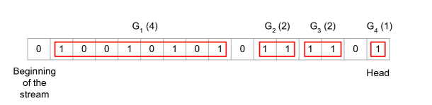
Figure 4.7: DGIM with parameter $B=1$. The head of the stream (the most recent element) is the rightmost bit. For each $k$, there are at least $B=1$ groups containing $2^{k}$ 1-bits, and at most $B+1=2$ groups containing $2^{k}$ 1-bits.

4.4.1 Updates

It is easy to see how to maintain the rules when a new bit arrives. If the bit is equal to 0, then nothing has to be done. If the bit is equal to 1, then:

1. Create a new group with the new bit.

2. If there are $B+2$ groups containing $2^{0}=1$ 1-bits, merge the two leftmost such groups so now there are $B$ groups containing one $1$-bit. This creates a new group containing $2^{1}=2$ 1-bits.

3. Repeat with the groups containing $2^{i}$ 1-bits, for $i=1,2,\dots$.

It is easy to see that one update step takes $O(\log m)$ worst-case time using doubly linked lists (this time is the delay of the algorithm). Define a global list $L=\ell_{q}\leftrightarrow\ell_{q-1}\leftrightarrow\dots\leftrightarrow\ell_{1}$. Element $\ell_{i}$ contains all the groups with $2^{i}$ 1-bits and is itself a doubly-linked list: $\ell_{i}=G_{j_{1}}\leftrightarrow\dots\leftrightarrow G_{j_{s}}$, where $G_{j_{1}},\dots,G_{j_{s}}$ are all the groups (listed from left to right in the stream) containing $2^{i}$ 1-bits. Each group $G_{j}$ is simply a pair of integers $G_{j}=(left,right)$: the leftmost and rightmost positions of the group in the stream. For each linked list $\ell_{i}$, we store its head, tail, number of stream’s bits contained in its groups, and number of ’1’-bits contained in its groups. Then, finding the leftmost two groups in a given $\ell_{i}$, merging them, and moving the merged group to the end of $\ell_{i+1}$ takes $O(1)$ time. Overall, an update takes therefore $O(q)=O(\log m)$ time.

Even better, updates take $O(1)$ amortized time. To see this, suppose that a particular update increases $Z_{k}$ by one unit (recall that $Z_{k}$ is the number of groups containing $2^{k}$ 1-bits). But then, this means that before that update $Z_{k^{\prime}}=B+1$ for all $k^{\prime}<k$. In turn, this configuration required $2^{k}-1$ previous updates, which added to the new update yields $2^{k}$ updates in total. This shows that only one over $2^{k}$ updates costs $k$: the amortized cost is therefore at most $\sum_{k=1}^{\infty}k/2^{k}=O(1)$.

4.4.2 Space and queries

The algorithm uses in total $O(\epsilon^{-1}\log^{2}m)$ bits of memory: each group uses $O(\log m)$ bits, and there are at most $B+1=O(\epsilon^{-1})$ groups containing $2^{k}$ 1-bits, for each $k=0,\dots,\log m$. The lists’ pointers also use asymptotically this space.

A query is specified by an integer $\bar{m}\leq m$ (the window size); our goal is to return the number of 1-bits contained in the most recent $\bar{m}$ bits of the stream. To solve a query, we simply find all the groups intersecting with (i.e. containing at least one of) the last $\bar{m}$ stream’s bits, and return the total number of $1$-bits they contain. This can be implemented by navigating the main list $\ell_{1}\rightarrow\ell_{2}\rightarrow\dots\rightarrow\ell_{i}$ until the number of bits contained in cells $\ell_{1},\ell_{2},\dots,\ell_{i}$ exceeds (or becomes equal to) $\bar{m}$. Then, we enter the cell $\ell_{i}$ and start navigating the linked list contained in $\ell_{i}$ until finding the leftmost group overlapping the last $\bar{m}$ stream’s characters. Finally, we add up all ’1’ bits contained in the cells $\ell_{1},\ell_{2},\dots,\ell_{i-1}$ and in the groups scanned in the last cell $\ell_{i}$. The total running time is $O(\epsilon^{-1}+\log\bar{m})$. Finally, if $\bar{m}$ is fixed then it is easy to see that queries take $O(1)$ time: at any time, we keep in memory only the groups overlapping with the last $\bar{m}$ stream’s bits (together with the total number of 1-bits that they contain). This also reduces the total space usage to $O(\epsilon^{-1}\log^{2}\bar{m})$ bits.

4.4.3 Approximation ratio

Next, we analyze the approximation ratio of the algorithm. Consider Figure 4.8, corresponding to the worst-case approximation ratio.

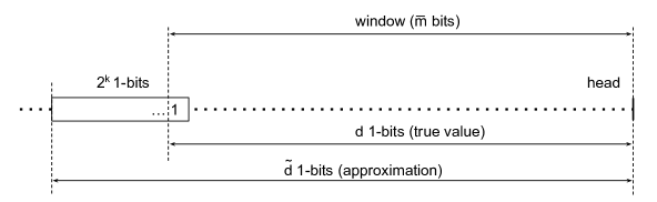
Figure 4.8: Worst case: our query (window of $\bar{m}$ bits) spans only the last bit of a block. The true number of 1-bits in the window is $d$. The answer we return ($\tilde{d}$) includes the whole block depicted on the left and containing $2^{k}$ ’1’-bits.

Let $k$ be the integer such that the leftmost (oldest) group intersecting the window has $2^{k}$ 1-bits. Let $d$ be the true number of 1-bits in the window, and $\tilde{d}$ be the sum of 1-bits in the groups intersecting the window (i.e. our approximate answer). If $k=0$, then it is easy to see that $\tilde{d}=d$ because every group intersecting the window contains 1 bit. We can therefore assume $k>0$. Clearly, $\tilde{d}\geq d$ since we count every block that overlaps with the window. We first compute a lower bound to $d$. Since the window spans a group containing $2^{k}$ 1-bits, then (by our invariants) the window surely contains at least $B$ groups containing $2^{j}$ 1-bits, for all $0\leq j<k$, i.e.

$$\begin{array}[]{rcl}d&\geq&B\cdot 2^{k-1}+B\cdot 2^{k-2}+\dots+B\cdot 2^{0}\\ &=&B\cdot(2^{k}-1)\end{array}$$

On the other hand, $\tilde{d}\leq d+2^{k}-1$ (in the worst case we have equality: this is the case in the example in Figure 4.8). We obtain:

$$\begin{array}[]{rcl}\frac{\tilde{d}}{d}&\leq&\frac{d+2^{k}-1}{d}\\ &=&1+\frac{2^{k}-1}{d}\\ &\leq&1+\frac{2^{k}-1}{B\cdot(2^{k}-1)}\\ &=&1+1/B\\ &\leq&1+\epsilon\end{array}$$

We conclude that $d\leq\tilde{d}\leq d\cdot(1+\epsilon)$.

The web page implements a very nice simulator of the DGIM algorithm (note that the stream’s head is on the left in this simulation).

4.4.4 Generalization: sum of integers

The algorithm can be used as a basis for many generalizations. Consider for example a stream formed by integers of $q$ bits each. We are interested in computing the sum of the last $\bar{m}$ integers in the stream.

The solution is to break the stream into $q$ parallel streams, one per bit in the integers: see Figure 4.9.

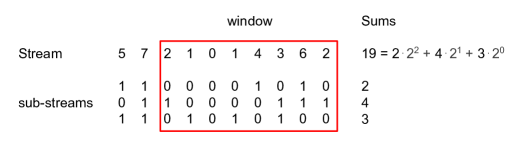
Figure 4.9: The sum of the last $\bar{m}$ $q$-bits integers can be reduced to the sum of the last $\bar{m}$ bits in the $q=3$ streams corresponding to the binary representations of the integers.

In other words: the $i$-th bit stream contains the binary weight of power $2^{i}$ in each integer of the original stream. Let $s_{i}$ be the sum of the $i$-th bit stream in the window. The correct answer is $d=\sum_{i=0}^{q-1}s_{i}2^{i}$. From the analysis of DGIM, we conclude that the answer $\tilde{d}$ we return is $d\leq\tilde{d}\leq\sum_{i=0}^{q-1}(1+\epsilon)s_{i}2^{i}=(1+\epsilon)\cdot d$.

Chapter 5 Exercises

The solutions of some of these exercises require techniques not described in these notes, see Section 0.1.

5.1 Information theory / compressed data structures

Exercise 5.1.1.

You are given a string $S\in\Sigma^{n}$ containing $r$ equal-letter runs. For example: if $S=AAABBBBCCAAA$, then $r=4$ (the four runs are $AAA$, $BBBB$, $CC$, and $AAA$. Design a data structure using $O(r)$ words of space able to answer rank and select queries on $S$ in $O(\log n)$ time. Bonus question: can you improve the space and query time of the data structure?

Exercise 5.1.2.

Design a compressed data structure implementing the following predictive text model. The data structure should store a string $S\in\Sigma^{n}$ in high-order entropy-compressed space and should be able to answer quickly the following query: given a substring $T$ of $S$, what is the character that follows $T$ in $S$ more frequently? For example, if $Ta$ appears 50 times in $S$, $Tb$ appears 10 times in $S$, and $Tc$ appears 123 times in $S$, then the answer is $c$.

Exercise 5.1.3.

Prove that you cannot encode in $n$ bits a set containing $n$ integers.

5.2 Data sketches

Exercise 5.2.1.

An embedded device with few KiB of RAM contains a sensor that measures the environment’s temperature (an integer number) every 10 seconds. We want to store all the generated data, in a streaming fashion, in a small-space sketch (note that the sensor produces several MiB of data per year). At any point in time, the data sketch should be able to answer quickly to the following query, with relative error $\epsilon$: what was the average temperature in a specific time range? (e.g. April 15th 2021, 10:15:40 AM - September 21th 2023, 09:10:20 PM).

Exercise 5.2.2.

We want to store a relational table $t(a_{1},a_{2},\dots,a_{k})$ in a small (polylogarithmic-space in the table’s size) sketch supporting the following two queries: (i) insert a new row into the table, and (ii) given $q$ attributes $a_{i_{1}},\dots,a_{i_{q}}$ at query time, estimate with relative error $\epsilon$ and failure probablity $\delta$ the number of distinct rows in the projection $\pi_{a_{i_{1}},\dots,a_{i_{q}}}(t)$.

Exercise 5.2.3.

We want to store a relational table $t(a_{1},a_{2},\dots,a_{k})$, where columns $a_{1},a_{2},\dots,a_{k}$ store integer numbers, in a small (polylogarithmic-space in the table’s size) sketch supporting the following two queries: (i) insert a new row into the table, and (ii) given an attribute $a_{i}$ and two integers $\ell\leq r$, estimate the number of rows (not necessarily distinct) such that $\ell\leq a_{i}\leq r$.

Exercise 5.2.4.

An embedded device with few KiB of RAM contains a GPS sensor that outputs the absolute position of a train (an integer number) on a railway every second. We want to store all the generated data, in a streaming fashion, in a small-space sketch. At any point in time, the data sketch should be able to answer quickly to the following query, with relative error $\epsilon$: what was the average speed of the train in a specific time range? (e.g. on April 15th 2021, from 10:15:45 AM to 12:10:22 PM).

Exercise 5.2.5.

Design an algorithm to be implemented on a router with few MiB of memory, to solve the following problem. We have the original code of a huge virus, occupying 1 GiB of space. To elude antivirus software, after infecting a new computer the virus modifies itself by swapping some characters from a small subset of fixed positions in the code (let’s say, 5 positions) that are unknown to us. Then, the infected computer sends the modified virus’ code on the network. Before and after sending the virus’ code, the infected computer could send other unrelated data. Assume that our router receives all packets passing through the network and, for simplicity, assume that IP packets are sorted by sender. Estimate how many computers have been infected.

Exercise 5.2.6.

Design an algorithm for a web crawler that explores the web and has the task to identify clusters of web pages being similar to each other, where similarity is measured according to the words contained in the web page.

Exercise 5.2.7.

You are hired at CIA with the task of preventing terrorist attacks. Design an algorithm to be implemented on a router with few KiB of memory, to estimate the number of IP addresses that issued Google searches for both these questions (possibly, the searches do not belong to the same IP packet): (i) where to buy ammonium-nitrate fertilizers, and (ii) how to activate a mechanical relay from distance with a mobile phone.

Exercise 5.2.8.

Design an algorithm to be implemented on a router with 3 GiB of free RAM, to solve the following problem: at any point in time, given an IPv4 address estimate how many IP packets have been sent from that address. You can assume that each IP address sends no more than $2^{63}$ IP packets. The answer must not exceed relative error $82\%$ with probability at least $1/4$.

Exercise 5.2.9.

Design an algorithm to be implemented on a router with 100 MiB of free RAM, to solve the following problem: at any point in time, given an IPv4 address estimate how many IP packets have been sent from that address. You can assume that the number of IP packets sent in total by all addresses does not exceed $2^{32}$. The answer must not exceed absolute error 1000.

Exercise 5.2.10.

Fix two IP addresses $IP_{1}$ and $IP_{2}$. Design an algorithm to be implemented on a router with few KiB of memory, to estimate the number of IP addresses that sent packets to both $IP_{1}$ and $IP_{2}$.

Bibliography

- [1] Noga Alon, Martin Dietzfelbinger, Peter Bro Miltersen, Erez Petrank, and Gábor Tardos. Linear hash functions. Journal of the ACM (JACM), 46(5):667–683, 1999.
- [2] Michael A Bender, Martin Farach-Colton, Rob Johnson, Bradley C Kuszmaul, Dzejla Medjedovic, Pablo Montes, Pradeep Shetty, Richard P Spillane, and Erez Zadok. Don’t thrash: how to cache your hash on flash. In 3rd Workshop on Hot Topics in Storage and File Systems (HotStorage 11), 2011.
- [3] Dany Breslauer and Zvi Galil. Real-time streaming string-matching. ACM Transactions on Algorithms (TALG), 10(4):1–12, 2014.
- [4] Andrei Z Broder. Min-wise independent permutations: Theory and practice. In International Colloquium on Automata, Languages, and Programming, pages 808–808. Springer, 2000.
- [5] Amit Chakrabarti. Data Stream Algorithms - Lecture Notes. https://www.cs.dartmouth.edu/~ac/Teach/data-streams-lecnotes.pdf. Accessed: 2023-01-03.
- [6] Raphaël Clifford, Allyx Fontaine, Ely Porat, Benjamin Sach, and Tatiana Starikovskaya. The k-mismatch problem revisited. In Proceedings of the twenty-seventh annual ACM-SIAM symposium on Discrete algorithms, pages 2039–2052. SIAM, 2016.
- [7] Raphaël Clifford, Tomasz Kociumaka, and Ely Porat. The streaming k-mismatch problem. In Proceedings of the Thirtieth Annual ACM-SIAM Symposium on Discrete Algorithms, pages 1106–1125. SIAM, 2019.
- [8] Graham Cormode. Data sketching. https://cacm.acm.org/magazines/2017/9/220427-data-sketching/fulltext. Communications of the ACM, 60(9):48–55, 2017.
- [9] Søren Dahlgaard, Mathias Bæk Tejs Knudsen, and Mikkel Thorup. Fast similarity sketching. In 2017 IEEE 58th Annual Symposium on Foundations of Computer Science (FOCS), pages 663–671. IEEE, 2017.
- [10] Mayur Datar, Aristides Gionis, Piotr Indyk, and Rajeev Motwani. Maintaining stream statistics over sliding windows. SIAM journal on computing, 31(6):1794–1813, 2002.
- [11] Marianne Durand and Philippe Flajolet. Loglog counting of large cardinalities. In European Symposium on Algorithms, pages 605–617. Springer, 2003.
- [12] Cristian Estan, George Varghese, and Mike Fisk. Bitmap algorithms for counting active flows on high speed links. In Proceedings of the 3rd ACM SIGCOMM conference on Internet measurement, pages 153–166, 2003.
- [13] Philippe Flajolet, Éric Fusy, Olivier Gandouet, and Frédéric Meunier. Hyperloglog: the analysis of a near-optimal cardinality estimation algorithm. In Discrete Mathematics and Theoretical Computer Science, pages 137–156. Discrete Mathematics and Theoretical Computer Science, 2007.
- [14] Philippe Flajolet and G Nigel Martin. Probabilistic counting. In 24th Annual Symposium on Foundations of Computer Science (sfcs 1983), pages 76–82. IEEE, 1983.
- [15] Seth Gilbert. CS5234 - Algorithms at Scale. https://www.comp.nus.edu.sg/~gilbert/CS5234/. Accessed: 2023-01-03.
- [16] Gregory Gundersen. Approximate Counting with Morris’s Algorithm. http://gregorygundersen.com/blog/2019/11/11/morris-algorithm/. Accessed: 2023-01-03.
- [17] Vibha Gupta, Maninder Singh, and Vinod K Bhalla. Pattern matching algorithms for intrusion detection and prevention system: A comparative analysis. In 2014 International Conference on Advances in Computing, Communications and Informatics (ICACCI), pages 50–54. IEEE, 2014.
- [18] Stefan Heule, Marc Nunkesser, and Alexander Hall. Hyperloglog in practice: Algorithmic engineering of a state of the art cardinality estimation algorithm. In Proceedings of the 16th International Conference on Extending Database Technology, pages 683–692, 2013.
- [19] Piotr Indyk. A small approximately min-wise independent family of hash functions. Journal of Algorithms, 38(1):84–90, 2001.
- [20] Mathias Bæk Tejs Knudsen. Linear hashing is awesome. In 2016 IEEE 57th Annual Symposium on Foundations of Computer Science (FOCS), pages 345–352. IEEE, 2016.
- [21] Jure Leskovec, Anand Rajaraman, and Jeffrey David Ullman. Mining of massive data sets. Cambridge university press, 2020.
- [22] Michael Mitzenmacher and Salil P Vadhan. Why simple hash functions work: exploiting the entropy in a data stream. In SODA, volume 8, pages 746–755. Citeseer, 2008.
- [23] Robert Morris. Counting large numbers of events in small registers. Communications of the ACM, 21(10):840–842, 1978.
- [24] Gonzalo Navarro. Compact data structures: A practical approach. Cambridge University Press, 2016.
- [25] Jelani Nelson. CS229r: Algorithms for Big Data. http://people.seas.harvard.edu/~minilek/cs229r/fall15/lec.html. Accessed: 2023-01-03.
- [26] Benny Porat and Ely Porat. Exact and approximate pattern matching in the streaming model. In 2009 50th Annual IEEE Symposium on Foundations of Computer Science, pages 315–323. IEEE, 2009.
- [27] Mihai Pǎtraşcu and Mikkel Thorup. The power of simple tabulation hashing. Journal of the ACM (JACM), 59(3):1–50, 2012.
- [28] Michael O Rabin. Fingerprinting by random polynomials. Technical report, 1981.
- [29] Rajeev Raman and Satti Srinivasa Rao. Succinct dynamic dictionaries and trees. In Jos C. M. Baeten, Jan Karel Lenstra, Joachim Parrow, and Gerhard J. Woeginger, editors, Automata, Languages and Programming, pages 357–368, Berlin, Heidelberg, 2003. Springer Berlin Heidelberg.
- [30] Ivan Stojmenovic and Amiya Nayak. Handbook of applied algorithms: Solving scientific, engineering, and practical problems. Chapter 8: Algorithms for Data Streams. http://www.dei.unipd.it/~geppo/PrAvAlg/DOCS/DFchapter08.pdf. John Wiley & Sons, 2007.