Mixed moving average field guided learning for spatio-temporal data

Abstract

Influenced mixed moving average fields are a versatile modeling class for spatio-temporal data. However, their predictive distribution is not generally known. Under this modeling assumption, we define a novel spatio-temporal embedding and a theory-guided machine learning approach that employs a generalized Bayesian algorithm to make ensemble forecasts. We employ Lipschitz predictors and determine fixed-time and any-time PAC Bayesian bounds in the batch learning setting. Performing causal forecast is a highlight of our methodology as its potential application to data with spatial and temporal short and long-range dependence. We then test the performance of our learning methodology by using linear predictors and data sets simulated from a spatio-temporal Ornstein-Uhlenbeck process.

MSC 2020: primary 60E07, 60E15, 60G25, 60G60; secondary 62C10.
Keywords: stationary models, weak dependence, randomized estimators, ensemble forecast, causal forecasts.

1 Introduction

Analyzing spatio-temporal data introduces various methodological challenges. These include determining models that can account for the serial correlation observed along their spatial and temporal dimensions and that, at the same time, can also enable forecasting tasks. Statistical models as Gaussian processes [6], [27], [62], and [73]; spatio-temporal kriging [24], and [53]; space-time autoregressive moving average models [35]; point processes [36], and hierarchical models [24] are very versatile in modeling the spatio-temporal correlation observed in the data and can deliver forecasts once the variogram or the data distribution (up to a set of parameters) is carefully chosen in relation to the studied phenomenon and practitioners’ experience. In a nutshell, such choices allow access to the models’ predictive distribution.

Suppose we want to avoid making any explicit choice regarding the data distribution. In this case, we can alternatively use deep learning methodologies to perform forecasting tasks in a spatio-temporal framework, see [5], [63], [71] and [72] for a review, or a video frame prediction algorithm as in [52] and [78]. Deep learning techniques can successfully extract spatio-temporal features and learn the inner law of an observed spatio-temporal system. However, these models lack interpretability, i.e., it is not possible to infer the correlation and causal relationship between variables in different space-time points that the models consider, and typically, no proof of their generalization performances is available in a spatio-temporal framework for dependent data. On the other hand, video prediction algorithms presented in [52] and [78] retain a causal interpretation of the relationship between different space-time points. However, as in the case of deep learning, we do not have proof of their generalization performances.

This paper proposes a novel theory-guided machine learning methodology for spatio-temporal data that enables one-time ahead ensemble forecasts based on moment assumptions (no further assumptions on the data distribution are needed), an opportune spatio-temporal embedding, and a generalized Bayesian algorithm. A theory-guided machine learning methodology is a hybrid procedure that employs a stochastic model in synergy with a learning algorithm. Such methodologies have started to gain prominence in several scientific disciplines such as earth science, quantum chemistry, bio-medical science, climate science, and hydrology modeling as, for example, described in [47], [59], [60], and [63]. In the following, we call our methodology mixed moving average field guided learning or MMAF-guided learning. Our methodology applies to raster data cubes [57], which are described for dimension $d=2$ in Section 3.1, and that are nowadays generated in environmental monitoring, from satellite observations, and climate and weather numerical models’ outputs. Our methodology applies, in general, to raster data having spatial dimension $d\geq 1$.

We assume that the data generating process is an influenced mixed moving average field (MMAF, in short), see Definition 2.6. Such a class of fields has been introduced in [26] and allows modeling the correlation and the causal relationship in different space-time points using ambit sets, see [8] [12] [54], and [55]. Such models have been so far employed to model data in environmental monitoring [41, 54], imaging analysis [46], and electricity networks [22]. They allow modeling Gaussian and non-Gaussian distributed data; they can be non-Markovian and have non-separable covariance functions. Moreover, they are stationary and $\theta$-lex weakly dependent [26] and allow modeling spatial and temporal short and long-range dependence. A drawback of employing MMAF in forecasting tasks is that their predictive distribution is not explicitly known. To our knowledge, the only available results on the predictive distribution of an MMAF in a spatio-temporal framework can be found in [54, Theorem 13] for a Gaussian spatio-temporal Ornstein-Uhlenbeck process.

We then define a randomized estimator (i.e., a regular conditional probability measure) on the class of the Lipschitz functions $\mathcal{H}$, see [38] for a review of this class of algorithms, based on the assumption that an MMAF generates the data. We call a function $h\in\mathcal{H}$ a predictor. Linear models, neural network architectures with feed-forward and convolutional modules [14, 69], and Lipschitz modifications of the transformer architecture [48, 58] are between the predictors belonging to $\mathcal{H}$. Our methodology applies when using a specific spatio-temporal embedding, i.e., we need to pre-process the observed data into a training data set $S_{m}$ on which the Lipschitz predictor can be learned. The precise construction of the spatio-temporal embedding is given in Section 3.1, along with the explanation of why choosing such embedding ensures a causal interpretation of the forecasts. Moreover, we prove PAC Bayesian bounds, which give us information about the generalization performance of any possible randomized estimators in the function of a selected spatio-temporal embedding. In particular, we analyze, in a simulation study, the performance of the randomized Gibbs estimator, which minimizes the bounds and has the best generalization performance in the estimators’ class.

1.1 Setting

Let $\boldsymbol{S}:=((\boldsymbol{X}_{i},\boldsymbol{Y}_{i})^{\top})_{i\in\mathbb{Z}}$ be a random vector where each $(\boldsymbol{X}_{i},\boldsymbol{Y}_{i})$ is identically distributed and has values in $\mathcal{X}\times\mathcal{Y}$ (Euclidean Spaces). We assume that $\boldsymbol{S}$ is a sample from an MMAF with finite second moments– a detailed definition is discussed in Section 3.1– which has a distribution $\mathbb{P}$ over the set $(\mathcal{X}\times\mathcal{Y})^{\mathbb{Z}}$, see [16] for a formal definition. We call a finite dimension realization of length $m$ from $\boldsymbol{S}$, a training data set and indicate it with $S_{m}:=((X_{i},Y_{i})^{\top})_{i=1}^{m}$ throughout. We also call $S:=((X_{i},Y_{i})^{\top})_{i\in\mathbb{Z}}$ a realization from $\boldsymbol{S}$.

Let $\mathcal{H}$ be the set of all Lipschitz functions $h:\mathcal{X}\to\mathcal{Y}$, and $L:\mathcal{X}\times\mathcal{Y}\to[0,\infty]$ a loss function. We define the generalization error (out-of-sample risk) as

$$R(h)=\mathbb{E}[L(h(\boldsymbol{X}),\boldsymbol{Y})],\$$ (1)

where $(\boldsymbol{X},\boldsymbol{Y})$ indicate a general example belonging to $\boldsymbol{S}$, and the empirical error (in-sample risk)

$$r(h)=\frac{1}{m}\sum_{i=1}^{m}L(h(X_{i}),Y_{i}).$$ (2)

The function $L$ is used to measure the discrepancy between a predicted output $h(\boldsymbol{X})$ and the true output $\boldsymbol{Y}$. Using the in-sample risk, we measure the performance of a given predictor $h$ just over an observed training data set $S_{m}$. In contrast, the out-of-sample risk gives us the performance of a predictor depending on the unknown distribution of the data $\mathbb{P}$. We then need a guarantee that a selected predictor will perform well when used on a set of out-of-sample observations, i.e., not belonging to $S_{m}$. We can also rephrase the problem as finding a predictor $h$ for which the difference between the out-of-sample and in-sample risk $R(h)-r(h)$ is as small as possible. We call the latter generalization gap. The classical PAC framework aims to find a bound on the generalization gap that holds with high probability $\mathbb{P}$; see, for example, [70] and [76]. Such probability inequality is also called a generalization bound. The acronym PAC stands for Probably Approximately Correct and may be traced back to [75]. A PAC inequality states that with an arbitrarily high probability (hence ”probably”), the performance (as provided by the generalization gap) of a learning algorithm is upper-bounded by a term decaying to an optimal value as more data is collected (hence ”approximately correct”).

We use in the paper a PAC Bayesian approach, also known as generalized Bayesian approach. First, we select a reference distribution $\pi$ on the space $(\mathcal{H},\mathcal{T})$, where $\mathcal{T}$ indicates a $\sigma$-algebra on the space $\mathcal{H}$. The reference distribution gives a structure on the space $\mathcal{H}$, which we can interpret as our belief that certain models will perform better than others. The choice of $\pi$, therefore, is an indirect way to make the size of $\mathcal{H}$ come into play; see [20, Section 3] for a detailed discussion on the latter point. Therefore, $\pi$ belongs to $\mathcal{M}_{+}^{1}(\mathcal{H})$, which denotes the set of all probability measures on the measurable set $(\mathcal{H},\mathcal{T})$. We then aim to determine a posterior distribution, also called a randomized estimator in the following, which is a regular conditional probability measure

$$\hat{\rho}:(\mathcal{X}\times\mathcal{Y})^{m}\times\mathcal{T}\to[0,1],$$

which satisfies the following properties:

• for any $A\in\mathcal{T}$, the map $S_{m}\to\hat{\rho}(S_{m},A):(\mathcal{X}\times\mathcal{Y})^{m}\to[0,1]$ is measurable;

• for any $S_{m}\in(\mathcal{X}\times\mathcal{Y})^{m}$, the map $A\to\hat{\rho}(S_{m},A):\mathcal{T}\to[0,1]$ is a probability measure in $\mathcal{M}_{+}^{1}(\mathcal{H})$.

From now on, we indicate with $\pi[\cdot]$, $\hat{\rho}[\cdot]$ the expectations with respect to the reference and posterior distributions. The latter is a conditional expectation w.r.t. $\boldsymbol{S_{m}}$, which in our notation represent the finite dimensional distribution of the process $\boldsymbol{S}$ generating the training data set. We simply indicate with $\mathbb{E}[\cdot]$ the expectation w.r.t. the probability distribution $\mathbb{P}$. Moreover, we call $\hat{\rho}[R(h)]$ and $\hat{\rho}[r(h)]$ the average generalization error and the average empirical error, respectively.

To evaluate the generalization performance of randomized estimators $\hat{\rho}$ on a class of predictors $\mathcal{H}$, we determine a so-called PAC Bayesian bound which is a bound on the (average) generalization gap defined as $\hat{\rho}[R(h)]-\hat{\rho}[r(h)]$ holding with high probability $\mathbb{P}$. PAC-Bayesian bounds have proven over the past two decades successful in addressing various learning problems such as classification, sequential or batch learning, and deep learning [33, 38].

MMAF-guided learning applies to bounded loss functions. Throughout, for $\epsilon>0$ called the accuracy level, we define the truncated absolute loss as

$$L^{\epsilon}(h(\boldsymbol{X}_{i}),\boldsymbol{Y}_{i}))=L(h(\boldsymbol{X}),\boldsymbol{Y}))\wedge\epsilon,$$ (3)

for all $i\in\mathbb{Z}$. The generalization error is then indicated with $R^{\epsilon}(h)=\mathbb{E}[L^{\epsilon}(h(\boldsymbol{X}),\boldsymbol{Y})]$ and the empirical error with $r^{\epsilon}(h)=\frac{1}{m}\sum_{i=1}^{m}L^{\epsilon}(h(X_{i}),Y_{i})$. The PAC Bayesian bounds in the paper are related to the average generalization gap $\hat{\rho}[R^{\epsilon}(h)]-\hat{\rho}[r^{\epsilon}(h)]$.

1.2 Contributions and Outline

The PAC Bayesian bounds proven in the paper are the first results in the literature for $\theta$-lex weakly dependent data, i.e., data generated by a stationary $\theta$-lex weakly dependent random field $\boldsymbol{Z}=(\boldsymbol{Z}_{t}(x))_{(t,x)\in\mathbb{R}\times\mathbb{R}^{d}}$. The latter is a novel notion of asymptotic independence introduced in [26]. When $\mathbb{E}[|\boldsymbol{Z}_{0}(0)|^{p}]<\infty$ for $p>1$, $\theta$-lex weak dependence is a more general notion than $\alpha_{\infty,v}$ and $\phi_{\infty,v}$-mixing for random fields being $v\in\mathbb{N}\cup\{\infty\}$, and $\alpha$ and $\phi$-mixing in the particular case of stochastic processes. In particular, an MMAF is a $\theta$-lex weakly dependent random field, which can then be used to model very general frameworks; see Remark 3.19 and Appendix A for a detailed discussion on this issue.

In the methodology we design, the dependence structure of an MMAF $\boldsymbol{Z}$ directly influences the selection of the Lipschitz predictor used in the forecasting tasks, which depends on the spatio-temporal embedding performed on the analyzed data (i.e., the training data set $S_{m}$). We select the latter such that the training data set inherits the $\theta$-lex weak dependence of the data generating process. Moreover, assessing the generalization performance of a predictor cannot be done empirically without an estimate of the decay rate of the $\theta$-lex coefficients of $\boldsymbol{Z}$. We give an exemplary application of our methodology in the case of the spatio-temporal Ornstein Uhlenbeck (STOU, in short) process and its mixed version called MSTOU processes defined in [54, 55], respectively. In the paper, we also discuss the range of applicability of such estimation methodology to other types of MMAFs.

To assess the generalization performance of a Lipschitz predictor, we prove a fixed-time and an any-time PAC Bayesian bound for $\theta$-lex weakly dependent spatio-temporal data. Our fixed-time PAC Bayesian bound holds for all training data sets $S_{m}$ with $m\geq 2$ and employs a novel exponential inequality for sums of weakly dependent processes. $\theta$-lex weak dependence is a notion of projective type related to an $L_{1}$-norm, see [26] and Remark A.1 and A.4. In regards to projective type dependence notions for $L_{p}$-norm and $p\in[1,\infty]$, there have been proven moment inequalities for partial sums of weakly dependent random fields in [17] for $p\in[2,\infty]$ and for stochastic processes and $p=1$ in [32]. To the best of our knowledge, another exponential inequality for a projective type dependence notion was obtained just for $p=\infty$ in [4](under the assumption that the $\theta_{1,\infty}$- coefficients are bounded).

There exist two comparable fixed-time bounds in the literature for dependent data that make explicit use of $\alpha$-mixing coefficients [2], which cannot be estimated from observed data, and $\theta_{1,\infty}$ bounded coefficients [4]. Both bounds apply to time series data and, therefore, to models that are not as general as the one represented by the class of MMAFs.

Regarding the any-time PAC Bayesian bound appearing in the paper, it is based on Ville’s maximal inequality for supermartingales [77] and it holds for all countable sequence of examples $S$, this means simultaneously for each $S_{m}$ and $m>0$. To give a complete overview of the range of applicability of MMAF-guided learning in the function of different choices of the training data set $S_{m}$ following the spatio-temporal embedding introduced in the paper, it is necessary to introduce both types of bounds. However, the any-time bound is of particular interest because it does not rely on the computation of the Lipschitz constant of the predictors. The latter is a significant point in evaluating the generalization performance of deep neural networks for which computing their Lipschitz constants is a complex numerical task; see [69] and [34]. Several any-time PAC Bayesian bounds exist in the literature for general dependent data frameworks as discussed in [39]. However, they do not hold in the so-called batch learning case for dependent data, which our proof covers for bounded losses. Moreover, we do not employ martingales in determining the bounds as done in [21] and [39]. We prove the bound simply by relying on the $\theta$-lex weakly dependence of the data generating process $\boldsymbol{Z}$.

The paper is structured as follows. First, we review the MMAF framework in Section 2 and describe its causal interpretation. In this section, we also introduce the STOU and MSTOU processes. These are isotropic random fields for which we compute novel bounds for their $\theta$-lex coefficients. The paper uses the latter to show feasible examples of MMAF-guided learning in the case of spatial and temporal short and long-range dependence. We introduce in Section 3 the spatio-temporal embedding applied to the data and the PAC Bayesian bounds for Lipschitz predictors. In Section 4, we discuss the causal interpretation of our forecasts and conclude by analyzing the performance of our methodology on six simulated data sets from an STOU process with a Gaussian and a normal-inverse-Gaussian distributed Lévy seed. Appendix A contains further details on the asymptotic independence notions discussed in the paper and a review of the estimation methodologies for STOU and MSTOU processes. Appendix B contains detailed proofs of the theoretical results presented in the paper.

2 Mixed moving average fields

2.1 Notations

Throughout the paper, we indicate with $\mathbb{N}$ the set of positive integers and $\mathbb{R}^{+}$ the set of non-negative real numbers. As usual, we write $L^{p}(\Omega)$ for the space of (equivalence classes of) measurable functions $f:\Omega\to\mathbb{R}$ with finite $L_{p}$-norm $\|f\|_{p}$. When $\Omega=\mathbb{R}^{n}$ and $x\in\Omega$, $\|x\|_{1}$ and $\lVert x\rVert$ denote the $L_{1}$-norm and the Euclidean norm, respectively, and we define $\lVert x\rVert_{\infty}=\max_{j=1,\ldots,n}|x^{(j)}|$, where $x^{(j)}$ represents the component $j$ of the vector $x$.

To ease the notations in the following sections, we sometimes indicate the index set $\mathbb{R}\times\mathbb{R}^{d}$ by $\mathbb{R}^{1+d}$. $A\subset B$ denotes a not necessarily proper subset $A$ of a set $B$, $|B|$ denotes the cardinality of $B$ and $dist(A,B)=\inf_{i\in A,j\in B}\lVert i-j\rVert_{\infty}$ indicates the distance of two sets $A,B\subset\mathbb{R}^{1+d}$. Let $n,k\geq 1$, and $F:\mathbb{R}^{n}\rightarrow\mathbb{R}^{k}$, we define $\lVert F\rVert_{\infty}=\sup_{t\in\mathbb{R}^{n}}\lVert F(t)\rVert$. Let $\Gamma=\{i_{1},\ldots,i_{u}\}\subset\mathbb{R}^{1+d}$ for $u\in\mathbb{N}$, we define the random vector $\boldsymbol{Z}_{\Gamma}=(\boldsymbol{Z}_{i_{1}},\ldots,\boldsymbol{Z}_{i_{u}})$. In general, we use bold notations when referring to random elements.

In the following, Lipschitz continuous is understood to mean globally Lipschitz. For $u\in\mathbb{N}$, $\mathcal{G}_{u}^{*}$ is the class of bounded functions from $\mathbb{R}^{u}$ to $\mathbb{R}$ and $\mathcal{G}_{u}$ is the class of bounded, Lipschitz continuous functions from $\mathbb{R}^{u}$ to $\mathbb{R}$ with respect to the distance $\|\cdot\|_{1}$ and define the Lipschitz constant as

$$Lip(h)=\sup_{x\neq y}\frac{|h(x)-h(y)|}{\|x-y\|_{1}}.$$ (4)

Hereafter, we often use the lexicographic order on $\mathbb{R}^{1+d}$. Let $t$ and $s$ be indicating a temporal and spatial coordinate. For distinct elements $y=(y_{1,t},y_{1,s}\ldots,y_{d,s})\in\mathbb{R}^{1+d}$ and $z=(z_{1,t},z_{1,s}\ldots,z_{d,s})\in\mathbb{R}^{1+d}$ we say $y<_{lex}z$ if and only if $y_{1,t}<z_{1,t}$ or $y_{p,s}<z_{p,s}$ for some $p\in\{1,\ldots,d\}$ and $y_{1,t}=z_{1,t}$ and $y_{q,s}=z_{q,s}$ for $q=1,\ldots,p-1$. Moreover, $y\leq_{lex}z$ if $y<_{lex}z$ or $y=z$ holds. Finally, let $z\in\mathbb{R}^{1+d}$, we define the set $V_{z}=\{y\in\mathbb{R}^{1+d}:y\leq_{lex}z\}$ and $V_{z}^{r}=V_{z}\cap\{y\in\mathbb{R}^{1+d}:\lVert z-y\rVert_{\infty}\geq r\}$ for $r>0$. The definition of the set $V_{z}^{r}$ is also used when referring to the lexicographic order on $\mathbb{Z}^{1+d}$.

2.2 Definition and properties of MMAF

Let $I=H\times\mathbb{R}\times\mathbb{R}^{d}$, where $H\subset\mathbb{R}^{q}$ for $q\geq 1$, and the Borel $\sigma$-algebra of $I$ be denoted by $\mathcal{B}(I)$ and let $\mathcal{B}_{b}(I)$ contain all its Lebesgue bounded sets.

Definition 2.1.

A family of $\mathbb{R}$-valued random variables $\Lambda=\{\Lambda(B):B\in\mathcal{B}_{b}(I)\}$ is called a Lévy basis on $(I,\mathcal{B}_{b}(I))$ if it is an independently scattered and infinitely divisible random measure. This means that:

• For a sequence of pairwise disjoint elements of $\mathcal{B}_{b}(I)$, say $\{B_{i},i\in\mathbb{N}\}$:

  • $\Lambda(\bigcup_{i\in\mathbb{N}}B_{i})=\sum_{i\in\mathbb{N}}\Lambda(B_{i})$ almost surely when $\bigcup_{i\in\mathbb{N}}B_{i}\in\mathcal{B}_{b}(I)$

  • and $\Lambda(B_{i})$ and $\Lambda(B_{j})$ are independent for $i\neq j$.

• Let $B\in\mathcal{B}_{b}(I)$. Then, the random variable $\Lambda(B)$ is infinitely divisible, i.e., for any $i\in\mathbb{N}$, there exists a law $\mu_{i}$ such that the law $\mu_{\Lambda(B)}$ can be expressed as $\mu_{\Lambda(B)}=\mu_{i}^{*i}$, the $i$-fold convolution of $\mu_{i}$ with itself.

For more details on infinitely divisible distributions, we refer the reader to [68]. In the following, we will restrict ourselves to Lévy bases which are homogeneous in space and time and factorizable, i.e., Lévy bases with characteristic function

$$\mathbb{E}\left[e^{\text{i}u\Lambda(B)}\right]=e^{\Phi(u)\Pi(B)}$$ (5)

for all $u\in\mathbb{R}$ and $B\in\mathcal{B}_{b}(I)$, where $\Pi=\pi\times\lambda_{1+d}$ is the product measure of the probability measure $\pi$ on $H$ and the Lebesgue measure $\lambda_{1+d}$ on $\mathbb{R}\times\mathbb{R}^{d}$. Note that when using a Lévy basis defined on $I=\mathbb{R}\times\mathbb{R}^{d}$, $\Pi=\lambda_{1+d}$. Furthermore,

$$\Phi(u)=\text{i}\gamma\,u-\frac{1}{2}\sigma^{2}u^{2}+\int_{\mathbb{R}}\left(e^{\text{i}ux}-1-\text{i}ux\boldsymbol{1}_{[0,1]}(|x|)\right)\nu(dx)$$ (6)

is the cumulant transform of an infinitely divisible distribution with characteristic triplet $(\gamma,\sigma^{2},\nu)$, where $\gamma\in\mathbb{R}$, $\sigma^{2}\geq 0$ and $\nu$ is a Lévy-measure on $\mathbb{R}$, i.e.,

$$\nu(\{0\})=0\quad\text{and}\int_{\mathbb{R}}\left(1\wedge x^{2}\right)\nu(dx)<\infty.$$

The quadruplet $(\gamma,\sigma^{2},\nu,\pi)$ determines the distribution of the Lévy basis, and therefore it is called its characteristic quadruplet. An important random variable associated with the Lévy basis, is the so-called Lévy seed, which we define as the random variable $\Lambda^{\prime}$ having as cumulant transform (6), that is

$$\mathbb{E}\left[e^{\text{i}u\Lambda^{\prime}}\right]=e^{\Phi(u)}.$$ (7)

By selecting different Lévy seeds, it is easy to compute the distribution of $\Lambda(B)$ for $B\in\mathcal{B}_{b}(I)$, for example, when $I=\mathbb{R}\times\mathbb{R}^{d}$. In the following two examples, we compute the Lévy bases used in generating the data sets in Section 4.1.

Example 2.2 (Gaussian Lévy basis).

Let $\Lambda^{\prime}\sim\mathcal{N}(\gamma,\sigma^{2})$, then its characteristic function is equal to $\exp(\text{i}\gamma u-\frac{1}{2}\sigma^{2}u^{2})$. Because of (5), we have, in turn, that the characteristic function of $\Lambda(B)$ is equal to $\exp(\text{i}\gamma u\lambda_{1+d}(B)-\frac{1}{2}\sigma^{2}\lambda_{1+d}(B)u^{2})$. In conclusion, $\Lambda(B)\sim\mathcal{N}(\gamma\lambda_{1+d}(B),\sigma^{2}\lambda_{1+d}(B))$ for any $B\in\mathcal{B}_{b}(I)$.

Example 2.3 (Normal Inverse Gaussian Lévy basis).

Let $K_{1}$ denote the modified Bessel function of the third order and index $1$. Then, for $x\in\mathbb{R}$, the NIG distribution is defined as

$$f(x:\alpha,\beta,\mu,\delta)=\alpha\delta(\pi^{2}(\delta^{2}+(x-\mu)^{2}))^{-\frac{1}{2}}\exp(\delta\sqrt{\alpha^{2}-\beta^{2}}+\beta(x-\mu))K_{1}(\alpha\sqrt{\delta^{2}+(x-\mu)^{2}}),$$

where $\alpha,\beta,\mu$ and $\delta$ are parameters such that $\mu\in\mathbb{R}$, $\delta>0$ and $0\leq|\beta|<\alpha.$ Let $\Lambda^{\prime}\sim NIG(\alpha,\beta,\mu,\delta)$, then by (5) we have that $\Lambda(B)\sim NIG(\alpha,\beta,\mu\lambda_{1+d}(B),\delta\lambda_{1+d}(B))$ for all $B\in\mathcal{B}_{b}(I)$.

We now follow [8], and [11] to formally define ambit sets.

Definition 2.4.

A family of ambit sets $(A_{t}(x))_{(t,x)\in\mathbb{R}\times\mathbb{R}^{d}}\subset\mathbb{R}\times\mathbb{R}^{d}$ satisfies the following properties:

$$\begin{cases}A_{t}(x)=A_{0}(0)+(t,x),\text{ (Translation invariant)}\\ A_{s}(x)\subset A_{t}(x),\,\,\text{for $s<t$}\\ A_{t}(x)\cap(t,\infty)\times\mathbb{R}^{d}=\emptyset\text{ (Non-anticipative)}.\end{cases}$$ (8)

We further assume that the random fields $\boldsymbol{Z}:=(\boldsymbol{Z}_{t}(x))_{(t,x)\in\mathbb{R}\times\mathbb{R}^{d}}$ in the paper are influenced. By this name we mean random fields defined on a given complete probability space $(\Omega,\mathcal{F},P)$, equipped with the filtration of influence (in the sense of Definition 3.8 in [26]) $\mathbb{F}=(\mathcal{F}_{(t,x)})_{(t,x)\in\mathbb{R}\times\mathbb{R}^{d}}$ generated by $\Lambda$ and the family of ambit sets $(A_{t}(x))_{(t,x)\in\mathbb{R}\times\mathbb{R}^{d}}\subset\mathbb{R}\times\mathbb{R}^{d}$, i.e., each $\mathcal{F}_{(t,x)}$ is the $\sigma$-algebra generated by the set of random variables $\{\Lambda(B):B\in\mathcal{B}_{b}(H\times A_{t}(x))\}$, which are adapted to $\mathbb{F}$. We call our field adapted to the filtration of influence $\mathbb{F}$ if it is measurable with respect to the $\sigma$-algebra $\mathbb{F}$ for each $(t,x)\in\mathbb{R}\times\mathbb{R}^{d}$.

Moreover, we work with stationary random fields in the following. We use the term stationary instead of spatio-temporal stationary.

Definition 2.5 (Spatio-temporal stationarity).

We say that $\boldsymbol{Z}$ is spatio-temporal stationary if for every $n\in\mathbb{N}$, $\tau\in\mathbb{R}$, $u\in\mathbb{R}^{d}$, $t_{1},\ldots,t_{n}\in\mathbb{R}$ and $x_{1},\ldots,x_{n}\in\mathbb{R}^{d}$, the joint distribution of $(\boldsymbol{Z}_{t_{1}}(x_{1}),\ldots,\boldsymbol{Z}_{t_{n}}(x_{n}))$ is the same as that of $(\boldsymbol{Z}_{t_{1}+\tau}(x_{1}+u),\ldots,\boldsymbol{Z}_{t_{n}+\tau}(x_{n}+u))$.

We can now formally define the stochastic model underlying our learning methodology.

Definition 2.6 (MMAF).

Let $\Lambda=\{\Lambda(B),B\in\mathcal{B}_{b}(I)\}$ a Lévy basis, $f:H\times\mathbb{R}\times\mathbb{R}^{d}\rightarrow\mathbb{R}$ a $\mathcal{B}(I)$-measurable function and $A_{t}(x)$ an ambit set. Then, the stochastic integral

$$\textbf{Z}_{t}(x)=\int_{H}\int_{A_{t}(x)}\,f(A,x-\xi,t-s)\,\,\Lambda(dA,d\xi,ds),\leavevmode\nobreak\ (t,x)\in\mathbb{R}\times\mathbb{R}^{d},$$ (9)

is adapted to the filtration $\mathbb{F}$, stationary, and its distribution is infinitely divisible. We call the $\mathbb{R}$-valued random field $\boldsymbol{Z}$ an (influenced) mixed moving average field and $f$ its kernel function.

Remark 2.7.

On a technical level, we assume all stochastic integrals in this paper to be well defined in the sense of Rajput and Rosinski [61]. For more details, including sufficient conditions on the existence of the integral as well as the explicit representation of the characteristic triplet of the MMAF’s infinitely divisible distribution (which can be directly determined from the characteristic quadruplet of $\Lambda$), we refer to [26, Section 3.1]. In the latter, there can also be found a multivariate definition of a Lévy basis and an MMAF.

Important examples of MMAFs are the spatio-temporal Ornstein-Uhlenbeck field (STOU) and the mixed spatio-temporal Ornstein-Uhlenbeck field (MSTOU), whose properties have been thoroughly analyzed in [54] and [55]. There are also interesting time series models in the MMAF framework, which we present in section A.5.

Example 2.8 (STOU process).

Let $\Lambda=\{\Lambda(B),B\in\mathcal{B}_{b}(I)\}$ be a Lévy basis, $f:\mathbb{R}\times\mathbb{R}^{d}\rightarrow\mathbb{R}$ a $\mathcal{B}(I)$-measurable function defined as $f(s,\xi)=\exp(-As)$ for $A>0$, and $A_{t}(x)$ be defined as in (12). Then, the STOU is defined as

$$\boldsymbol{Z}_{t}(x):=\int_{A_{t}(x)}\exp(-A(t-s))\Lambda(ds,d\xi).$$ (10)

The STOU is then a stationary and Markovian random field. Moreover, an STOU exhibits exponential temporal autocorrelation (just like the temporal Ornstein-Uhlenbeck process) and has a spatial autocorrelation structure determined by the shape of the ambit set. In addition, this class of fields admits non-separable autocovariances, which are desirable in practice, see Example A.8.

Example 2.9 (MSTOU process).

An MSTOU process is defined by mixing the parameter $A$ in the definition of an STOU process; that is, we assume that $A$ is a random variable with support in $H=(0,\infty)$. This modification allows the determination of random fields with power-decaying autocovariance functions, see example A.10. Let $\Lambda=\{\Lambda(B),B\in\mathcal{B}_{b}(I)\}$ be a Lévy basis, $f:(0,\infty)\times\mathbb{R}\times\mathbb{R}^{d}\rightarrow\mathbb{R}$ a $\mathcal{B}(I)$-measurable function defined as $f(A,s,\xi)=\exp(-As)$, and $A_{t}(x)$ be defined as in (12). Moreover, let $l(A)$ be the density of $\pi$ with respect to Lebesgue measure such that

$$\int_{0}^{\infty}\frac{1}{A^{d+1}}l(A)dA<\infty.$$

Then, the MSTOU is defined as

$$\boldsymbol{Z}_{t}(x):=\int_{0}^{\infty}\int_{A_{t}(x)}\exp(-A(t-s))\Lambda(dA,ds,d\xi).$$ (11)

The MMAF framework has a causal interpretation under the following assumption.

Assumption 2.10.

For a $c>0$, we consider

$$A_{t}(x):=\big{\{}(s,\xi)\in\mathbb{R}\times\mathbb{R}^{d}:s\leq t\,\,\textit{and}\,\,\|x-\xi\|\leq c|t-s|\big{\}}.$$ (12)

To explain why using cone-shaped ambit sets allows to have such interpretation, we borrow the concept of lightcone from special relativity.

A lightcone describes the possible paths that the light can make in space-time leading to a space-time point $(t,x)$ and the ones that lie in its future. In the context of our paper, we use their geometry to identify the space-time points having a causal relationship. For a point $(t,x)$, $c>0$ and by using the Euclidean norm to assess the distance between different space-time points, we define a lightcone as the set

$$\mathcal{A}^{light}_{t}(x)=\big{\{}(s,\xi)\in\mathbb{R}\times\mathbb{R}^{d}:\|x-\xi\|\leq c|t-s|\big{\}}.$$

The set $\mathcal{A}^{light}_{t}(x)$ can be split into two disjoint sets, namely, $A_{t}(x)$ and $A_{t}(x)^{+}$. The set $A_{t}(x)$ is called past lightcone, and its definition corresponds to the one of a cone-shaped ambit set (12).

The set

$$A_{t}(x)^{+}=\{(s,\xi)\in\mathbb{R}\times\mathbb{R}^{d}:s>t\,\textrm{and}\,\,\|x-\xi\|\leq c|t-s|\},$$ (13)

is called instead the future lightcone. By using an influenced MMAF on a cone-shaped ambit set as the underlying model, we implicitly assume that the following sets

$$l^{-}(t,x)=\{Z_{s}(\xi):(s,\xi)\in A_{t}(x)\setminus(t,x)\}\,\,\,\textrm{and}\,\,\,l^{+}(t,x)=\{Z_{s}(\xi):(s,\xi)\in A_{t}(x)^{+}\}$$ (14)

are respectively describing the values of the field that have a direct influence on the determination of $\boldsymbol{Z}_{t}(x)$ and the future field values influenced by $\boldsymbol{Z}_{t}(x)$. We can then uncover the causal relationship between space-time points described above by estimating the constant $c$ from observed data, which we call the speed of information propagation in the physical system under analysis. A similar approach to the modeling of causal relationships can be found in several machine learning frameworks, as in [52], [67], and [78]. In [52] and [67], the sets (14) are considered and employed to discover coherent structures [44] in spatio-temporal physical systems and to perform video frame prediction, respectively. In [78], forecasts are performed by embedding spatio-temporal information on a Minkowski space-time. Hence, the concept of lightcones enters into play in the definition of their algorithm. In statistical modeling, we typically have two equivalent approaches towards causality: structural causal models, which rely on the use of directed acyclical graphs (DAG) [56], and Rubin causal models, which rely upon the potential outcomes framework [66]. The concept of causality employed in this paper can be inscribed into the latter. In fact, by using MMAFs on cone-shaped ambit sets, the set $l^{+}(t,x)$ describes the possible future outcomes that can be observed starting from the spatial position $(t,x)$.

Finally, we consider the following definitions of spatial and temporal short and long-range dependence in the paper.

Definition 2.11 (Short and long range dependence).

A random field $(\boldsymbol{Z}_{t}(x))_{(t,x)\in\mathbb{R}\times\mathbb{R}^{d}}$ is said to have temporal short-range dependence if

$$\int_{0}^{\infty}Cov(\boldsymbol{Z}_{t}(x),\boldsymbol{Z}_{t+\tau}(x))\,\,d\tau<\infty,$$

and temporal long-range dependence if the integral above is infinite. Similarly, an isotropic random field, see Definition A.11, has spatial short-range dependence if

$$\int_{0}^{\infty}C(r)\,\,dr<\infty,$$

where $Cov(\boldsymbol{Z}_{t}(x),\boldsymbol{Z}_{t}(x+u))=C(|u|)$ and $r=|u|$. It is said to have spatial long-range dependence if the integral is infinite.

Under Assumption 2.10, an STOU process admits temporal and spatial short-range dependence, whereas an MSTOU process can admit temporal and spatial short and long-range dependence by carefully modeling the random parameter $A$.

Example 2.12.

Let $\boldsymbol{Z}$ be an MSTOU process as defined in Example 2.9 for $d=1$, Assumption 2.10 hold, and $l(A)=\frac{\beta^{\alpha}}{\Gamma(\alpha)}A^{\alpha-1}\exp(-\beta A)$ be the Gamma density with shape and rate parameters $\alpha>d+1$ and $\beta>0$. From the calculations in Example A.10 and by setting $u=0$, then $\boldsymbol{Z}$ has temporal short-range dependence for $\alpha>3$, because

$$\int_{0}^{\infty}Cov(\boldsymbol{Z}_{t}(x),\boldsymbol{Z}_{t+\tau}(x))\,d\tau =\frac{c\beta^{\alpha}Var(\Lambda^{\prime})}{2(\alpha-2)(\alpha-1)}\int_{0}^{\infty}(\beta+\tau)^{-(\alpha-2)}\,d\tau$$

$$=\frac{c\beta^{3}Var(\Lambda^{\prime})}{2(\alpha-1)(\alpha-2)(\alpha-3)}.$$

This integral is infinite for $2<\alpha\leq 3$, and the process has temporal long-range dependence. We obtain spatial short or long-range dependence for the same choice of parameters. In fact, for $r=|u|$ and $\tau=0$, and $\alpha>3$

$$\int_{0}^{\infty}C(r)\,dr =\frac{c\beta^{\alpha}Var(\Lambda^{\prime})}{2(\alpha-2)(\alpha-1)}\int_{0}^{\infty}(\beta+r/c)^{-(\alpha-2)}\,dr$$

$$=\frac{c\beta^{3}Var(\Lambda^{\prime})}{2(\alpha-1)(\alpha-2)(\alpha-3)},$$

converges, whereas the integral diverges for $2<\alpha\leq 3$.

2.3 Weak dependence coefficients in MMAF guided learning

MMAFs are $\theta$-lex weakly dependent random fields. For $v\in\mathbb{N}\cup\{\infty\}$, the latter is a dependence notion more general than $\alpha_{\infty,v}$-mixing, see Lemma A.5.

Definition 2.13.

Let $\boldsymbol{Z}$ be an $\mathbb{R}$-valued random field. Then, $\boldsymbol{Z}$ is called $\theta$-lex-weakly dependent if

$$\theta_{lex}(r)=\sup_{u,v\in\mathbb{N}}\theta_{u,v}(r)\underset{r\rightarrow\infty}{\longrightarrow}0,$$

where

$$\theta_{u,v}(r)=\sup\bigg{\{}\frac{|Cov(F(\boldsymbol{Z}_{\Gamma}),G(\boldsymbol{Z}_{\Gamma^{\prime}}))|}{\lVert F\rVert_{\infty}vLip(G)}\bigg{\}}$$

and $F\in\mathcal{G}^{*}_{u},G\in\mathcal{G}_{v}$; $\Gamma=\{t_{i_{1}},\ldots,t_{i_{u}}\}\subset\mathbb{R}^{1+d}$, $\Gamma^{\prime}=\{t_{j_{1}},\ldots,t_{j_{v}}\}\subset\mathbb{R}^{1+d}$ such that $|\Gamma|=u$, $|\Gamma^{\prime}|=v$ and $\Gamma\subset V_{\Gamma^{\prime}}^{r}=\bigcap_{l=1}^{v}V_{t_{j_{l}}}^{r}$ for $t_{j_{l}}\in\Gamma^{\prime}$. We call $(\theta_{lex}(r))_{r\in\mathbb{R}^{+}}$ the $\theta$-lex-coefficients.

The latter is an extension to the random field case of a dependence notion developed for causal processes called $\theta$-lex weak dependence.

Definition 2.14.

Let $\boldsymbol{Z}$ be an $\mathbb{R}$-valued stochastic process. Then, $\boldsymbol{Z}$ is called $\theta$-weakly dependent if

$$\theta(k)=\sup_{u\in\mathbb{N}}\theta_{u}(k)\underset{k\rightarrow\infty}{\longrightarrow}0,$$

where

$$\theta_{u}(k)=\sup\bigg{\{}\frac{|Cov(F(\boldsymbol{Z}_{\Gamma}),G(\boldsymbol{Z}_{j_{1}}))|}{\lVert F\rVert_{\infty}Lip(G)}\bigg{\}}.$$

and $F\in\mathcal{G}_{u}^{*},G\in\mathcal{G}_{1}$; $\Gamma=\{i_{1},\ldots,i_{u}\}\subset\mathbb{R}$ such that $i_{1}\leq i_{2}\leq\ldots\leq i_{u}\leq i_{u}+k\leq j_{1}$. We call $(\theta(k))_{k\in\mathbb{R}^{+}}$ the $\theta$-coefficients.

Remark 2.15 (About the parameter $k$ and $r$ in Definition 2.14 and 2.13).

Let us start by assuming that $\boldsymbol{Z}=(\boldsymbol{Z}_{i})_{i\in\mathbb{R}}$ is a sequence of independent and identically distributed (in short, i.i.d.) random vectors, then for any $F\in\mathcal{G}_{u}^{*}$ with $u\in\mathbb{N}$, $G\in\mathcal{G}_{1}$, and selecting a set $\Gamma=\{i_{1},\ldots,i_{u}\}\subset\mathbb{R}$ such that $i_{1}\leq\ldots\leq i_{u}\leq i_{u}+k\leq j$, we have that

$$Cov(F(\boldsymbol{Z}_{\Gamma}),G(\boldsymbol{Z}_{i_{u}}))=0,$$

and $\theta(k)=0$ for all $k\in\mathbb{R}^{+}$. The process $\boldsymbol{Z}$ is $\theta$-weakly dependent and the parameter $k$ is encoding the distance between the marginals

$$\boldsymbol{P}:=(\boldsymbol{Z}_{i_{1}},\ldots,\boldsymbol{Z}_{i_{u}}),\,\,\,\textrm{and}\,\,\,\boldsymbol{F}:=(\boldsymbol{Z}_{j}).$$

In terms of the process $\boldsymbol{Z}$, the $\sigma$-algebras generated by $\boldsymbol{P}$ and $\boldsymbol{F}$ represent past and future events. Obviously, in the case of a sequence of independent random variables, the past plays no role in the unfolding of the future. Let us assume now that when $\boldsymbol{Z}$ is $\theta$-weakly dependent such that

$$Cov(F(\boldsymbol{Z}_{i_{1}},\ldots,\boldsymbol{Z}_{i_{u}}),G(\boldsymbol{Z}_{j}))\leq 2\|F\|_{\infty}Lip(G)\theta(k).$$

The above inequality proven in [25] makes the asymptotic independence between past and future. Here, the past is progressively forgotten for $k\to\infty$ explicit. The parameter $k$ expresses the distance at which we are evaluating the influence of the past on how the future unfolds, and the coefficients $\theta(k)$ is a measure of how fast the past is forgotten.

Similar considerations can be done in the case in which we consider $\boldsymbol{Z}=(\boldsymbol{Z}_{i})_{i\in\mathbb{R}^{1+d}}$ a $\theta$-lex weakly dependent random field about the constant $r\in\mathbb{R}^{+}$. However, $\boldsymbol{P}$ and $\boldsymbol{F}$ represent the marginals of lexicographically ordered elements in this case. The lexicographic order in $\mathbb{R}^{1+d}$ substitutes the natural temporal order for stochastic processes defined on $\mathbb{R}$.

In the MMAF modeling framework, we can show general formulas for the computation of upper bounds of the $\theta$-lex coefficients. The latter is given as a function of the characteristic quadruplet of the driving Lévy basis $\Lambda$ and the kernel function $f$ in (9), see Proposition B.1.

For $d=1,2$, when the MMAF has a kernel function with no spatial component, we can compute a bound for the $\theta$-lex coefficients expressed in terms of the covariances of the field $\boldsymbol{Z}$, which can be computed as shown in Section A.2. These bounds have an expression that allows us to use standard statistical inference tools to infer their decay rate parameter; see, for example, the estimators (16) and (17). In the general framework described in Proposition B.1, however, similar estimation methodologies are not yet available and remain an interesting open problem.

Proposition 2.16.

Let $\Lambda$ be an $\mathbb{R}$-valued Lévy basis with characteristic triplet $(\gamma,\sigma^{2},\nu,\pi)$ and $f:H\times\mathbb{R}\rightarrow\mathbb{R}$ a $\mathcal{B}(H\times\mathbb{R})$-measurable function not depending on the spatial dimension, i.e.,

$$\boldsymbol{Z}_{t}(x)=\int_{H}\int_{A_{t}(x)}f(A,t-s)\Lambda(dA,ds,d\xi),\quad(t,x)\in\mathbb{R}^{1+d}.$$ (15)

1. For $d=1$, if $\int_{|x|>1}x^{2}\nu(dx)<\infty$ and $\gamma+\int_{|x|>1}x\nu(dx)=0$, then $\boldsymbol{Z}$ is $\theta$-lex weakly dependent and

   $$\theta_{lex}(r)\! \leq\!2\left(\!2Var(\Lambda^{\prime})\int_{0}^{\infty}\int_{A_{0}(0)\cap A_{0}(r\min(2,c))}\!\!f(A,-s)^{2}dsd\xi\pi(dA)\right)^{1/2}$$

   $$=\!2\sqrt{2Cov(\boldsymbol{Z}_{0}(0),\boldsymbol{Z}_{0}(r\min(2,c)))},$$

   where $Var(\Lambda^{\prime})=\sigma^{2}+\int_{\mathbb{R}}x^{2}\,\nu(dx)$.

2. For $d=2$, if $\int_{|x|>1}x^{2}\nu(dx)<\infty$ and $\gamma+\int_{|x|>1}x\nu(dx)=0$, then $\boldsymbol{Z}$ is $\theta$-lex weakly dependent and

   $$\theta_{lex}(r) \leq 2\Bigg{(}2Cov\left(\boldsymbol{Z}_{0}(0,0),\boldsymbol{Z}_{0}\left(r\min\left(1,\frac{c}{\sqrt{2}}\right),r\min\left(1,\frac{c}{\sqrt{2}}\right)\right)\right)$$

   $$\qquad+2Cov\left(\boldsymbol{Z}_{0}(0,0),\boldsymbol{Z}_{0}\left(r\min\left(1,\frac{c}{\sqrt{2}}\right),-r\min\left(1,\frac{c}{\sqrt{2}}\right)\right)\right)\Bigg{)}^{1/2}.$$

The proof of the results above is given in Appendix B.1.

Notation 2.17.

In general, we indicate the bounds of the $\theta$-lex coefficients determined in Proposition B.1, Corollary B.2 or Proposition 2.16 using the sequence $(\tilde{\theta}_{lex}(r))_{r\in\mathbb{R}^{+}}$ where

$$\theta_{lex}(r)\leq 2\tilde{\theta}_{lex}(r).$$

Example 2.18.

Let $d=1$ and $\boldsymbol{Z}$ be an STOU as in Definition 2.8. If $\int_{|x|>1}x^{2}\,\nu(dx)<\infty$, $\gamma+\int_{|x|>1}x\,\nu(dx)=0$, then $\boldsymbol{Z}$ is $\theta$-lex weakly dependent with

$$\tilde{\theta}_{lex}(r) =\Big{(}Var(\Lambda^{\prime})\int_{A_{0}(0)\cap(A_{0}(\psi)\cup A_{0}(-\psi))}\exp(2As)\,ds\,d\xi\Big{)}^{\frac{1}{2}}$$

$$\leq\Big{(}2Var(\Lambda^{\prime})\int_{A_{0}(0)\cap A_{0}(\psi)}\exp(2As)\,ds\,d\xi\Big{)}^{\frac{1}{2}}$$

$$=\Big{(}2Var(\Lambda^{\prime})\int_{-\infty}^{-\frac{\psi}{2c}}\int_{\psi+cs}^{-cs}\exp(2As)\,ds\,d\xi\Big{)}^{\frac{1}{2}}=\Big{(}\frac{c}{A^{2}}Var(\Lambda^{\prime})\,\exp\Big{(}\frac{-A\psi}{c}\Big{)}\Big{)}^{\frac{1}{2}}$$

$$=\Big{(}\,\frac{c}{A^{2}}Var(\Lambda^{\prime})\,\exp\Big{(}-\,\underset{2\lambda}{\underbrace{\frac{A\min(2,c)}{c}}}\,r\Big{)}\Big{)}^{\frac{1}{2}}$$

$$=\sqrt{2Cov(\boldsymbol{Z}_{0}(0),\boldsymbol{Z}_{0}(r\min(2,c)))}:=\bar{\alpha}\exp(-\lambda r),$$

where $\lambda>0$ and $\bar{\alpha}>0$. Because the temporal and spatial autocovariance functions of an STOU are exponential, see (44), the model admits spatial and temporal short-range dependence.

By estimating the parameter vector $\theta_{0}=\{A,c,Var(\Lambda^{\prime})\}$ using the methodologies revised in Appendix A.3, we can estimate the parameter $\lambda$ using the following plug-in estimator

$$\boldsymbol{\lambda^{*}}=\frac{\min(2,\boldsymbol{c^{*}})}{2\boldsymbol{c^{*}}},$$ (16)

where the estimators $\boldsymbol{A^{*}}$ and $\boldsymbol{c^{*}}$ are defined in (59). This estimator is consistent because of [54, Theorem 12] and the continuous mapping theorem. Furthermore, by using an estimator of the parameter $Var(\Lambda^{\prime})$, we can also obtain a consistent estimator for the parameter $\bar{\alpha}$.

Example 2.19.

Let $d=1$ and $\boldsymbol{Z}$ be an MSTOU as defined in Example 2.12. If $\int_{|x|>1}x^{2}\,\nu(dx)<\infty$, $\gamma+\int_{|x|>1}x\,\nu(dx)=0$, then $\boldsymbol{Z}$ is $\theta$-lex weakly dependent with

$$\tilde{\theta}_{lex}(r) \leq\Big{(}\frac{c}{A^{2}}Var(\Lambda^{\prime})\,\int_{0}^{\infty}\exp\Big{(}\frac{-A\psi}{c}\Big{)}\pi(dA)\Big{)}^{\frac{1}{2}}$$

$$=\Big{(}\frac{Var(\Lambda^{\prime})c\beta^{\alpha}}{(\beta+\psi/c)^{\alpha-2}(\alpha-2)(\alpha-1)}\Big{)}^{\frac{1}{2}}$$

$$=\Big{(}\frac{Var(\Lambda^{\prime})c\beta^{\alpha}}{(\alpha-2)(\alpha-1)}\Big{(}\beta+\frac{r\min(2,c)}{c}\Big{)}^{-(\alpha-2)}\Big{)}^{\frac{1}{2}}$$

$$=\sqrt{2Cov(\boldsymbol{Z}_{0}(0),\boldsymbol{Z}_{0}(r\min(2,c)))}:=\bar{\alpha}r^{-\lambda},$$

where $\lambda=\frac{\alpha-2}{2}$ and $\bar{\alpha}>0$. As already addressed in Example 2.12, for $2<\alpha\leq 3$, that is $0<\lambda\leq\frac{1}{2}$, the model admits temporal and spatial long-range dependence. Instead, for $\alpha>3$, that is $\lambda>\frac{1}{2}$, the model admits temporal and spatial short range dependence.

For the model used in Example 2.19, an estimator for

$$\boldsymbol{\lambda}^{*}=\frac{\boldsymbol{\alpha}^{*}-2}{2}$$ (17)

where the vector of parameters $\theta_{1}=\{\alpha,\beta,c,Var(\Lambda^{\prime})\}$ is estimated using a GMM estimator $\boldsymbol{\theta}_{1}^{*}=\{\boldsymbol{\alpha}^{*},\boldsymbol{\beta}^{*},\boldsymbol{c}^{*},\boldsymbol{Var(\Lambda^{\prime})}^{*}\}$.

The estimator of $\lambda$ depends on the chosen data generating process and the spatial dimension of the data. For further details on the parametric estimation methodologies nowadays available for other fields belonging to the MMAF class, we refer the reader to the Appendices A.3, A.4 and A.5.

3 Mixed moving average field guided learning

3.1 Pre-processing $N$ frames

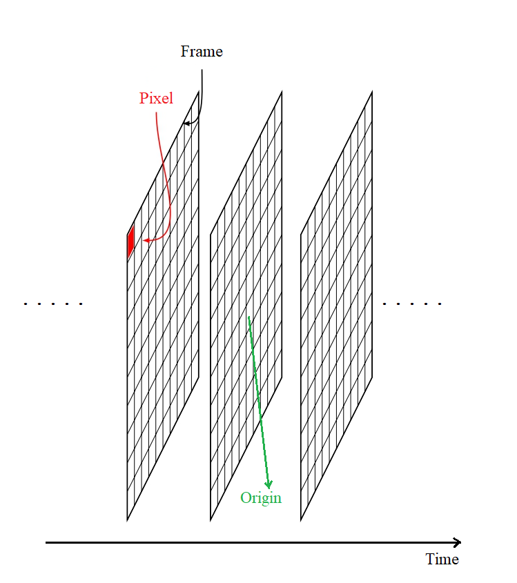
Figure 1: Raster data cube’s spatio-temporal index set with origin in $(t_{0},x_{0})$.

In this section, we describe MMAF-guided learning for a spatial dimension $d=2$. Let $(\tilde{Z}_{t}(x))_{(t,x)\in\mathbb{T}\times\mathbb{L}}$ be an observed data set on a regular lattice $\mathbb{L}\subset\mathbb{R}^{2}$ across times $\mathbb{T}=\{t_{0}+h_{t},\ldots,t_{0}+h_{t}N\}$ for $h_{t}\in\mathbb{R}$, such that

$$\tilde{Z}_{t}(x)=\mu_{t}(x)+Z_{t}(x)$$ (18)

holds and no measurement errors are present in the observations. Here, $\mu_{t}(x)$ is a deterministic function, and $Z_{t}(x)$ are considered realizations from a zero mean stationary (influenced) MMAF.

We represent graphically the regular spatial lattice $\mathbb{L}$ as a frame made of a finite amount of pixels, i.e., squared-cells representing each of them a unique spatial position $x\in\mathbb{L}$, see Figure 1.In several applications, such as satellite imagery, a pixel refers to a spatial cell of several square meters. In the paper, we assume that a pixel represents the spatial point $x\in\mathbb{R}^{2}$ corresponding to the center of the pictured squared cell. We then use the name pixel and spatial position throughout interchangeably. In total, $N$ frames represent the spatio-temporal index set of the observed data set. This terminology is often used to describe raster data cubes [57]. We apply below the spatio-temporal embedding described in Section 3.1.1 to data with such structure. For dimension $d=1$, we consider that the pixel collapses in the point $x\in\mathbb{R}$ that describes, see Figure 3. MMAF-guided learning also applies to spatial index set of dimension $d>2$. However, we do not represent the spatial positions using pixels in such cases.

We call $(t_{0},x_{0})$ the origin of the space-time grid, see Figure 1, and $h_{t}$ and $h_{s}$ the time and space discretization step in the observed data set, i.e. the distance between two pixels along the temporal and spatial dimensions.

Mixed moving average guided learning (MMAF guided learning, in short) has the target to determine one-time ahead ensemble forecasts of the field $\boldsymbol{Z}$ in a pixel $x^{*}$. We do not consider further the problem of estimating the deterministic function $\mu_{t}(x)$ when performing forecasting tasks, i.e., we assume our data set to be generated by a zero mean MMAF from now on. We refer the reader to [24] for a review of how to estimate the function $\mu_{t}(x)$.

We need to work with a training data set to employ a learning algorithm in the following sections. Therefore, we pre-process the set of indices represented by the $N$ frames to select a set of different examples, i.e., input-output pairs, to define a training data set $S_{m}$ starting from $(Z_{t}(x))_{(t,x)\in\mathbb{T}\times\mathbb{L}}$.

3.1.1 Spatio-temporal embedding

Let us consider a stationary random field $(\boldsymbol{Z}_{t}(x))_{(t,x)\in\mathbb{Z}\times\mathbb{L}}$, and select a pixel position $x^{*}$ in $\mathbb{L}$. We define the input-output vectors

$$\boldsymbol{X}_{i}=\boldsymbol{L^{-}_{p}}(t_{0}+ia,x^{*}),\,\,\,\,\textrm{and}\,\,\,\,\,\boldsymbol{Y}_{i}=\boldsymbol{Z}_{t_{0}+ia}(x^{*}),\,\,\,\textrm{for $i\in\mathbb{Z}$},$$ (19)

where

$$\boldsymbol{L^{-}_{p}}(t,x^{*})=(\boldsymbol{Z}_{i_{1}}(\xi_{1}),\ldots,\boldsymbol{Z}_{i_{a(p,c)}}(\xi_{a(p,c)}))^{\top},$$ (20)

with indices selected in the set

$$\mathcal{I}(t,x^{*}):=\{(i_{s},\xi_{s}):\|x^{*}-\xi_{s}\|\leq c\,(t-i_{s})\,\, \textrm{for}\,\,0<t-i_{s}\leq p,$$

$$\textrm{and}\,\,(i_{s},\xi_{s})<_{lex}(i_{s+1},\xi_{s+1})\},$$ (21)

for $t=t_{0}+ia$ with $i\in\mathbb{Z}$, and $c>0$. We call $a(p,c):=|\mathcal{I}(t,x^{*})|$ and assume that it is constant for all $t=t_{0}+ia$ and $i\in\mathbb{Z}$. The parameters $a>0$ and $p>0$ are multiples of $h_{t}$ such that $a=a_{t}h_{t}$, $p=p_{t}h_{t}$, $a_{t},p_{t}\in\mathbb{N}$ and $a_{t}\geq p_{t}+1$. We note that each element of $L^{-}_{p}(t,x^{*})\subset l^{-}(t,x^{*})$ for $t=t_{0}+ia$ and $i\in\mathbb{Z}$, where $l^{-}(t,x^{*})$ is defined in (14) and identifies the set of all points in $\mathbb{R}\times\mathbb{R}^{d}$ that could possibly influence the realization $Z_{t}(x^{*})$. The sampling leading to (19) can be performed starting by a pixel $x^{*}$ for which the index set $\mathcal{I}(t_{0}+ia,x^{*})\subseteq\mathbb{Z}\times\mathbb{L}$ for all $i$. Further details on why the examples need to be structured following the index sets $\mathcal{I}(t,x^{*})$ are given in the next remark.

Remark 3.1 (Geometry and lexicographic order of the examples).

The sets $\mathcal{I}(t,x^{*})$ are chosen with a geometry that is inherited by the definition of the cone-shaped ambit set in (12). Such a geometry allows us to give a causal interpretation of the one-time ahead ensemble forecast, as shown in Section 4. Moreover, we store in the vectors $\boldsymbol{X_{i}}$ values of the fields $\boldsymbol{Z}$ with indices in lexicographic order. This choice implies that $((\boldsymbol{X}_{i_{1}},\boldsymbol{Y}_{i_{1}}),\ldots,(\boldsymbol{X}_{i_{u}},\boldsymbol{Y}_{i_{u}}))$ and $(\boldsymbol{X}_{j},\boldsymbol{Y}_{j})$ for $u\in\mathbb{N}$ and $j\in\mathbb{R}^{i+d}$ are lexicographically ordered marginals of the field $\boldsymbol{Z}$. This allows, in turn, to precisely assess how the $\theta$-lex weakly dependence of the data generating process $\boldsymbol{Z}$ (defined w.r.t. lexicographically ordered marginals, see Definition 2.13) is inherited by the process $\boldsymbol{S}$ and to understand how the $\theta$-lex weakly dependence plays a role in the definition of the algorithms in Section 3.2. Modifications of this representation may be needed when using convolutional or transformer architectures as predictors. This latter issue is outside the scope of the present paper but constitutes an important future research direction of MMAF-guided learning.

Last but not least, it is important to notice that the considerations above rule out the choice of overlapping examples, i.e., the possible choice of examples that maintain the cone-shaped geometry but have indices not following the lexicographic order. If we were to make this choice, we would then work with a training data set that does not inherit the dependence structure of the data generating process $\boldsymbol{Z}$; see Section 3.1.2 for more details.

The sequence $((\boldsymbol{X}_{i},\boldsymbol{Y}_{i})^{\top})_{i\in\mathbb{Z}}$ is composed of identically distributed random vectors for all $i\in\mathbb{Z}$. We call $\boldsymbol{S}:=((\boldsymbol{X}_{i},\boldsymbol{Y}_{i})^{\top})_{i\in\mathbb{Z}}$ a cone-shaped sampling process. An example of a realization $S$ of the sampling scheme can be found in Figure 2. The distribution of $\boldsymbol{S}$ is indicated throughout by $\mathbb{P}$.

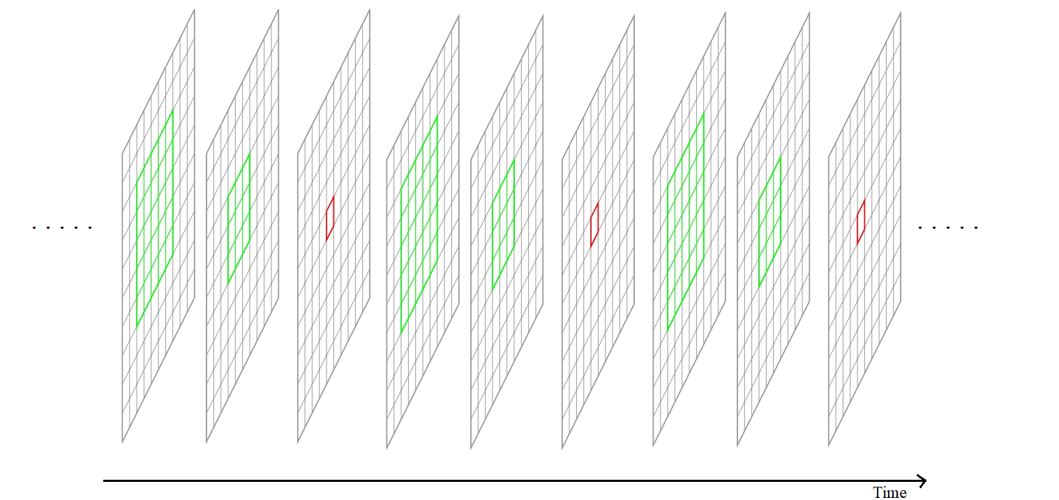
Figure 2: We follow the notations of (20). The red pixel identifies the spatial point $x^{*}$. For $i\in\mathbb{Z}$ the set $\mathcal{I}(t_{0}+ia,x^{*})$ defined in (3.1.1) is represented by the green pixels. The parameters in use in this sampling are $c=\sqrt{2}$, $p_{t}=2$, $a_{t}=3$, $h_{t}=h_{s}=1$.

Next, let us assume to observe a data set $(Z_{t}(x))_{(t,x)\in\mathbb{T}\times\mathbb{L}}$, and that we want to determine a one-time ahead ensemble forecast in the pixel $x^{*}$. We define $m:=\Big{\lfloor}\frac{N}{a_{t}}\Big{\rfloor}$ and a training data set $S_{m}=((X_{i},Y_{i})^{\top}))_{i=1}^{m}$ as a realization from the cone-shaped sampling process $\boldsymbol{S}$ of fixed length $m$. In particular,

$$X_{i}=L^{-}_{p}(t_{0}+ia,x^{*}),\,\,\,\,\textrm{and}\,\,\,\,\,Y_{i}=Z_{t_{0}+ia}(x^{*})\,\,\,\,\textrm{for $i=1,\ldots,m$},$$ (22)

where

$$L^{-}_{p}(t,x^{*})=(Z_{i_{1}}(\xi_{1}),\ldots,Z_{i_{a(p,c)}}(\xi_{a(p,c)}))^{\top},\,\,\,\textrm{and $(i_{s},\xi_{s})\in\mathcal{I}(t,x^{*})$}$$ (23)

for $s=1,\ldots,a(p,c)$ and $t=t_{0}+ia$ with $i=1,\ldots,m$. We assume that the parameters $a$ and $p$ follow the constraints in Table 1. The index set selected to define the training data set (22) is a spatio-temporal embedding in the set $\mathbb{R}\times\mathbb{R}^{2}$. A similar interpretation can be given for the index set defining the cone-shaped sampling process (19).

Parameters	Constraints	Interpretation
$a:=a_{t}h_{t}$	$p_{t}+1\leq a_{t}\leq\Big{\lfloor}\frac{N}{2}\Big{\rfloor}$	translation vector
$p:=p_{t}h_{t}$	$1\leq p_{t}<\Big{\lfloor}\frac{N}{2}\Big{\rfloor}-1$	past time horizon
$m:=\frac{N}{a_{t}}$	$2<m<N$	number of examples in $S_{m}$

Table 1: Parameters involved in pre-processing $N$ observed frames.

For an observed raster data cube, we know the value of the constants $N$, $h_{t}$, and $h_{s}$, and it remains to select the parameters $a_{t}$ and $p_{t}$. We discuss the selection of the parameter $a_{t}$ in Section 3.2 and of $p_{t}$ in Section 4.1, respectively.

3.1.2 Asymptotic independence of the stochastic processes $\boldsymbol{L}$ and $\boldsymbol{L}^{\epsilon}$

We prove in this section the asymptotic independence of the processes $\boldsymbol{L}:=(L(h(\boldsymbol{X}_{i}),\boldsymbol{Y}_{i}))_{i\in\mathbb{Z}}$ and $\boldsymbol{L^{\epsilon}}:=(L^{\epsilon}(h(\boldsymbol{X}_{i}),\boldsymbol{Y}_{i}))_{i\in\mathbb{Z}}$, for the loss functions $L$ and $L^{\epsilon}$ defined in Section 1.1, and $h$ a Lipschitz predictor.

Proposition 3.2.

Let $\boldsymbol{S}$ be the cone-shaped sampling process defined by (19), then for all $h\in\mathcal{H}$, $\boldsymbol{L}$ is a $\theta$-weakly dependent process. Moreover, for $a,p>0$, $k\in\mathbb{N}$, and $r=ka-p>0$, it has coefficients

$$\theta(k)\leq\tilde{d}(Lip(h)a(p,c)+1)\Big{(}\frac{2}{\tilde{d}}\mathbb{E}[|\boldsymbol{Z}_{t}(x)-\boldsymbol{Z}_{t}^{(r)}(x)|]+\theta_{lex}(r)\Big{)},$$ (24)

where $\tilde{d}>0$ is a constant independent of $r$, and $\boldsymbol{Z}_{t}^{(r)}(x):=\boldsymbol{Z}_{t}(x)\wedge r$.

Remark 3.3 (Locally Lipschitz predictor).

Let the predictor $h$ be a locally Lipschitz function such that $h(0)=0$ and

$$|h(x)-h(y)|\leq\tilde{c}\,\|x-y\|_{1}(1+\|x\|_{1}+\|y\|_{1})\,\,\textrm{for $x,y\in\mathbb{R}^{a(p,c)}$},$$

for $\tilde{c}>0$. Moreover, let $\boldsymbol{Z}$ be a stationary and $\theta$-lex weakly dependent random field such that $|\boldsymbol{Z}|\leq C$ almost surely. An easy generalization of Proposition 3.2, leads to show that $\boldsymbol{L}$ is $\theta$-weakly dependent with coefficients

$$\theta(k)\leq\tilde{d}(\tilde{c}(1+2C)a(p,c)+1)\Big{(}\frac{2}{\tilde{d}}\mathbb{E}[|\boldsymbol{Z}_{t}(x)-\boldsymbol{Z}_{t}^{(r)}(x)|]+\theta_{lex}(r)\Big{)},$$ (25)

where $r=ka-p>0$ for $a,p>0$ and $k\in\mathbb{N}$, $\tilde{d}>0$ is a constant independent of $r$, and $\boldsymbol{Z}_{t}^{(r)}(x):=\boldsymbol{Z}_{t}(x)\wedge r$.

Remark 3.4.

The spatio-temporal embedding discussed in Section 3.1.1 also apply to $\theta$-weakly dependent time series models $\boldsymbol{Z}$. In such case, the parameter $c=0$, $\boldsymbol{S}$ is a flat cone-shaped sampling process, and (straightforwardly) a $\theta$-weakly dependent process with coefficients satisfying the bound (24).

In the case of MMAFs, we have obtained explicit bounds for the coefficients $\theta_{lex}(r)$ in Propositions B.1 and 2.16. We now prove that a more refined bound than (24) for the $\theta$-coefficients of the process $\boldsymbol{L}$ can be given in this setting.

We consider the following assumption.

Assumption 3.5.

Let $\boldsymbol{Z}$ be an MMAF under the Assumption 2.10 and such that $\mathbb{E}[|\boldsymbol{Z}_{t}(x)|^{2}]<\infty$. Let $N\in\mathbb{N}$, $\mathbb{T}=\{t_{0}+h_{t},\ldots,t_{0}+h_{t}N\}$ and $\mathbb{L}\subset\mathbb{R}^{2}$, then $S_{m}$ and $S$ are realization from $(\boldsymbol{Z}_{t}(x))_{(t,x)\in\mathbb{Z}\times\mathbb{L}}$ following the spatio-temporal embeddings defined,respectively, in Section 3.1.1.

Proposition 3.6.

Let Assumption 3.5 hold. Then $\boldsymbol{L}$ is $\theta$-weakly dependent for all $h\in\mathcal{H}$ with coefficients

$$\theta(k)\leq 2(Lip(h)a(p,c)+1)\widetilde{\theta}_{lex}(r),$$ (26)

where $r=ka-p>0$ for $a,p>0$ and $k\in\mathbb{N}$. In particular, for linear predictors, i.e., $h_{\beta}(X)=\beta_{0}+\beta_{1}^{T}X,\,\textrm{for}\,\,\beta:=(\beta_{0},\beta_{1})^{\top}\in B$ and $B=\mathbb{R}^{a(p,c)+1}$, we have that $\boldsymbol{L}$ is $\theta$-weakly dependent for all $\beta\in B$ with coefficients

$$\theta(k)\leq 2(\|\beta_{1}\|_{1}+1)\widetilde{\theta}_{lex}(r).$$ (27)

Lemma A.3 straightforwardly implies that the process $\boldsymbol{L}^{\epsilon}$ is $\theta$-weakly dependent with the same $\theta$-coefficients as the process $\boldsymbol{L}$ under the assumptions of Proposition 3.2, Remark 3.3 and Proposition 3.6.

3.2 PAC Bayesian bounds for MMAF generated data

Three essential building blocks, namely the change of measure theorem of Donsker and Varadhan [31], the Markov’s inequality, and an exponential inequality are typically employed to prove a fixed-time PAC Bayesian bound. The latter is so called because it holds for a given choice of $m$ (which in our framework is related to a given number $N$ of frames).

First of all, let us define the Kullback-Leibler divergence, which is defined as

$$KL(\rho||\pi)=\left\{\begin{array}[]{ll}\rho\Big{[}\log\frac{d\rho}{d\pi}\Big{]}&\textrm{if}\,\,\,\rho<<\pi\\ +\infty&\textrm{otherwise}\end{array}\right.$$

for a given measurable space $(\mathcal{H},\mathcal{T})$ and for any $(\rho,\pi)\in\mathcal{M}_{+}^{1}(\mathcal{H})^{2}$, where $\rho<<\pi$ means that $\rho$ is absolutely continuous respect to $\pi$ with Radon-Nikodym derivative $\frac{d\rho}{d\pi}$. We prove next an exponential inequality for $\theta$-weakly dependent processes using the notations introduced in Section 3.1.

Theorem 3.7.

Let $\boldsymbol{Z}$ be an $\mathbb{R}$-valued stationary $\theta$-weakly dependent process, and $f:\mathbb{R}\to[a,b]$, for $a,b\in\mathbb{R}$ such that $(f(\boldsymbol{Z}_{i}))_{i\in\mathbb{Z}}$ is itself $\theta$-weakly dependent. Let $l=\lfloor\frac{m}{k}\rfloor$, for $m,k\in\mathbb{N}$, such that $l\geq 2$ and $0<s<\frac{3l}{|b-a|}$, then

$$\mathbb{E}\Big{[}\exp\Big{(}\frac{s}{m}\sum_{i=1}^{m}(f(\boldsymbol{Z}_{i})-\mathbb{E}[f(\boldsymbol{Z}_{i})])\Big{)}\Big{]}\leq\exp\Bigg{(}\frac{s^{2}Var(f(\boldsymbol{Z}_{1}))}{2l\Big{(}1-\frac{s|b-a|}{3l}\Big{)}}\Bigg{)}+\exp(s\,|b-a|)\theta(k)s,$$ (28)

$$\mathbb{E}\Big{[}\exp\Big{(}\frac{s}{m}\sum_{i=1}^{m}(\mathbb{E}[f(\boldsymbol{Z}_{i})]-f(\boldsymbol{Z}_{i}))\Big{)}\Big{]}\leq\exp\Bigg{(}\frac{s^{2}Var(f(\boldsymbol{Z}_{i}))}{2l\Big{(}1-\frac{s|b-a|}{3l}\Big{)}}\Bigg{)}+\exp(s\,|b-a|)\theta(k)s.$$ (29)

Note that increasing the parameter $k$ makes the bounds in (28) and (29) become tighter because $\theta(k)$ goes to zero when $k$ goes to infinity.

We have shown in the last section that the process $\boldsymbol{L}^{\epsilon}$ is $\theta$-weakly dependent, then Theorem 3.7 allows us to determine a fixed-time PAC Bayesian bound.

Theorem 3.8 (PAC Bayesian bound).

Let $0<\epsilon<3$, $l=\Big{\lfloor}\frac{m}{k}\Big{\rfloor}$ such that $l\geq 2$, $r=ka-p$, and $\pi$ be a distribution on $\mathcal{H}$ such that $\pi[Lip(h)]<\infty$. If Assumption 3.5 holds, then for any $\hat{\rho}$ such that $\hat{\rho}<<\pi$, and $\delta\in(0,1)$

$$\mathbb{P}\Big{\{}|\hat{\rho}[R^{\epsilon}(h)] -\hat{\rho}[r^{\epsilon}(h)]|\leq\Big{(}KL(\hat{\rho}||\pi)+\log\Big{(}\frac{1}{\delta}\Big{)}+\frac{3\epsilon^{2}}{2(3-\epsilon)}\Big{)}\frac{1}{\sqrt{l}}$$

$$+\frac{1}{\sqrt{l}}\log\Big{(}\pi\Big{[}1+2(Lip(h)a(p,c)+1)3\sqrt{l}\exp(3\sqrt{l})\theta(k)\Big{]}\Big{)}\Big{\}}\geq 1-2\delta.$$ (30)

For any possible choice of the parameters defining the spatio-temporal embedding leading to $\boldsymbol{S}_{m}$, Theorem 3.8 gives us a PAC Bayesian bound for a randomized estimator $\hat{\rho}$. We remark that the bigger the parameter $k$, the smaller the $\theta$-lex coefficients appear in the bound and the slower the convergence rate of the bound’s right-hand side (in the function of the parameter $m$). The fastest convergence rate that can be obtained in this framework is $\mathcal{O}(m^{1/2})$ when choosing the parameter $k=1$. Possible choices of the spatio-temporal embedding can be found in the remark below.

Remark 3.9 (About the choice of $\sqrt{l}$ and the spatio-temporal embedding).

Differently from the classical PAC Bayesian i.i.d. (namely, independent and identically distributed) setting, see reviews [1] and [38], the parameter $l$ is not tuned in the bounds (30). The value of the parameter $l$ depends on the spatio-temporal embedding chosen. We now give several exemplary spatio-temporal embedding using throughout Notation 2.17 and considering the parameter $p_{t}$ a hyperparameter.

For $k=1$, we obtain a convergence rate of $\mathcal{O}(m^{\frac{1}{2}})$, and we can pre-process the data choosing the parameter

$$\left\{\begin{array}[]{ll}a_{t}>\frac{3\sqrt{N}+\lambda h_{t}p_{t}}{h_{t}\lambda}&\textrm{if $\boldsymbol{Z}$ admits exp. decaying $\theta$-lex coef.}\\ a_{t}>\frac{\exp(3\sqrt{N}/\lambda)+h_{t}p_{t}}{h_{t}}&\textrm{if $\boldsymbol{Z}$ admits power decaying $\theta$-lex coef.}\end{array}\right.$$

Under these choices, we obtain that $\exp(3\sqrt{l})\tilde{\theta}_{lex}(r)\leq 1$, and the bound (30) tightens. By choosing $k>1$, i.e., a less sparse sampling, and

$$\left\{\begin{array}[]{ll}a_{t}>\frac{3\sqrt{N}+\lambda h_{t}p_{t}}{k\lambda h_{t}}&\textrm{if $\boldsymbol{Z}$ admits exp. decaying $\theta$-lex coef.}\\ a_{t}>\frac{\exp(3\sqrt{N}/\lambda)+h_{t}p_{t}}{kh_{t}}&\textrm{if $\boldsymbol{Z}$ admits power decaying $\theta$-lex coef.}\end{array}\right.$$

we obtain that the average generalization gap converges to zero with a rate $\mathcal{O}(\sqrt{m/k})$. We can also choose a sparser sampling scheme such that $3\sqrt{l}\exp(3\sqrt{l})\tilde{\theta}_{lex}(r)\leq 1$, which will tighten the bound even more. For example, for $k=1$, we can choose

$$\left\{\begin{array}[]{ll}a_{t}>\frac{3\sqrt{N}+\log(3\sqrt{N})+\lambda h_{t}p_{t}}{h_{t}\lambda}&\textrm{if $\boldsymbol{Z}$ admits exp. decaying $\theta$-lex coef.}\\ a_{t}>\frac{\exp(3\sqrt{N}/\lambda+\log(3\sqrt{N})/\lambda)+h_{t}p_{t}}{h_{t}}&\textrm{if $\boldsymbol{Z}$ admits power decaying $\theta$-lex coef.}\end{array}\right.$$ (31)

It is important to highlight that the choice of the parameter $a_{t}$ in the spatio-temporal embeddings discussed in this section is inversely proportional to the parameter $k$ and proportional to the parameter $p_{t}$. This means we obtain more examples (i.e., longer training data sets $S_{m}$) when $k$ increases and $p_{t}$ decreases. Hence, a careful choice of the parameter $a_{t}$ must be done even to obtain training data sets with $m\geq 1$. Tuning all the parameters involved in the pre-processing step is especially important for data showing temporal long-range dependence.

Remark 3.10 (Feasible methodology to determine $a_{t}$ following the rules in Remark 3.9).

When the field $\boldsymbol{Z}$ is an MMAF having a kernel independent on the spatial dimension, the parameters $c$ and $\lambda$ can be estimated from the entire observed data set $(Z_{t}(x))_{(t,x)\in\mathbb{T}\times\mathbb{L}}$. For the STOU and MSTOU processes we review the estimation methodology for their parameters in the Sections A.3 and A.4, respectively. In Examples 2.18 and 2.19, we find the estimators for the parameter $\lambda$ and $c$ when $d=1$.

Example 3.11.

Let us pre-process the data following the selection of the parameter $a_{t}$ (31) in the case of linear predictors. The bound (30) holds for all randomized estimators $\hat{\rho}$ absolutely continuous w.r.t. a reference distribution $\pi$ given a training data set $S_{m}$. Let us assume that $B:=\{\beta:\|\beta\|_{1}\leq 1\}$ and $card(B)=M$ for $M\in\mathbb{N}$. We choose throughout as reference distribution the uniform distribution $\pi$ on $B$ and the class of randomized estimator $\hat{\rho}=\delta_{\boldsymbol{\hat{\beta}}}$, the Dirac mass concentrated on the empirical risk minimizer, i.e., $\hat{\beta}:=arg\inf_{\beta}r^{\epsilon}(\beta)$. For a given $S$, we have that

$$KL(\delta_{\hat{\beta}}||\pi)=\sum_{\beta\in B}\log\Big{(}\frac{\delta_{\hat{\beta}}\{\beta\}}{\pi\{\beta\}}\Big{)}\delta_{\hat{\beta}}\{\beta\}=\log\frac{1}{\pi\{\hat{\beta}\}}=\log(M).$$ (32)

It is crucial to notice that the bigger the cardinality of the space $B$ is, the more the term $\log(M)$ and the bound increase.

Therefore, using the bound (27) for the $\theta$ coefficients of the process $\boldsymbol{L}^{\epsilon}$, for $\delta\in(0,1)$

$$\mathbb{P}\Big{\{}R^{\epsilon}(\hat{\beta})\leq r^{\epsilon}(\hat{\beta})+\Big{(}\log\Big{(}\frac{M}{\delta}\Big{)}+\frac{3\epsilon^{2}}{2(3-\epsilon)}\Big{)}\frac{1}{\sqrt{l}}+\frac{1}{\sqrt{l}}\log\Big{(}\pi[1+2(\|\beta_{1}\|_{1}+1)\bar{\alpha}]\Big{)}\Big{\}}\geq 1-\delta.$$

Let us assume to work with an accuracy level $\epsilon=1$, $l=10000$, $M=100$, $\bar{\alpha}=4$, $\delta=0.05$. Then, the generalization gap is less than $0.12$ with probability $\mathbb{P}$ of at least $95\%$.

We now focus on determining an any-time PAC Bayesian bound, which is so-called because it holds simultaneously for every $m$. Let us define for $\epsilon>0$, the process

$$\left\{\begin{array}[]{l}f_{0}(\boldsymbol{S},h)=0\\ f_{m}(\boldsymbol{S},h):=\eta\sum_{i=1}^{m}(L^{\epsilon}(h(X_{i}),Y_{i})-\mathbb{E}[L^{\epsilon}(h(\boldsymbol{X}_{i}),\boldsymbol{Y}_{i})])+\eta^{2}m\theta_{lex}^{Decay}(k),\,\,\textrm{for $m\in\mathbb{N}$},\end{array}\right.$$

where

$$\theta_{lex}^{Decay}(k):=\left\{\begin{array}[]{ll}\log(\exp(-\lambda h_{t}(ka_{t}-p_{t}))&\textrm{if $\boldsymbol{Z}$ admits exp. decaying $\theta$-lex coef.}\\ \log((h_{t}(a_{t}-p_{t}))^{-\lambda})&\textrm{if $\boldsymbol{Z}$ admits power decaying $\theta$-lex coef.}\end{array}\right.$$

represents the decay of the exponential or power function appearing in the $\theta_{lex}(r)$ coefficient of the process $\boldsymbol{Z}$ for $r=ka-p$, where $a,p>0$ and $k\in\mathbb{N}$. We aim to prove that the process

$$A_{m}:=\pi[\exp(f_{m}(\boldsymbol{S},h))]$$ (33)

is a supermartingale with respect to the filtration generated by the cone-shaped sampling process $\boldsymbol{S}$.

The proof of Theorem 3.12 differs from the results proven in [21] and [39]. In particular, we do not employ a sub $\psi$-process condition as in the proof of Corollary 4.1. in [21]. Moreover, in our framework, the generalization gap (multiplied by m) is not a martingale as in [39]. As in the proofs already existing for identically distributed and dependent random variables, we apply Ville’s inequality for non-negative supermartingale [77] and avoid the use of the Markov’s inequality in the standard scheme of proof for PAC Bayesian bounds given in [13].

Theorem 3.12.

Let $\pi$ be a distribution on $\mathcal{H}$. If Assumption 3.5 holds and $-\theta_{lex}^{Decay}(k)>2\epsilon$ for $\epsilon>0$, then for any $\hat{\rho}<<\pi$, $m>0$, $\eta>0$ and $\delta\in(0,1)$

$$\mathbb{P}\Big{\{}|\hat{\rho}[R^{\epsilon}(h)]-\hat{\rho}[r^{\epsilon}(h)]|\leq\Big{(}KL(\hat{\rho}||\pi)+\log\Big{(}\frac{1}{\delta}\Big{)}\Big{)}\frac{1}{m\eta}-\eta\theta_{lex}^{Decay}(k)\Big{\}}\geq 1-2\delta.$$ (34)

Remark 3.13 (Data pre-processing and spatio-temporal embedding for the any-time bound).

A novelty of the above theorem is that the bound holds simultaneously on all $m>0$ as long as we pre-process the data as in the theorem’s assumption. For $k=1$, we have that $a_{t}>\frac{2\epsilon}{\lambda h_{t}}+p_{t}$ when the field $\boldsymbol{Z}$ admits exponentially decaying $\theta$-lex coefficients or $a_{t}>\frac{\exp(2\epsilon/\lambda)}{h_{t}}+p_{t}$ when the field $\boldsymbol{Z}$ admits power decaying $\theta$-lex coefficients. Note that, the training data set with the higher amount of examples for $k=1$ is obtained for

$$\left\{\begin{array}[]{ll}a_{t}=\lceil\frac{2\epsilon}{\lambda h_{t}}+p_{t}\rceil&\textrm{if $\boldsymbol{Z}$ admits exp. decaying $\theta$-lex coef.}\\ a_{t}=\lceil\frac{\exp(2\epsilon/\lambda)}{h_{t}}+p_{t}\rceil&\textrm{if $\boldsymbol{Z}$ admits power decaying $\theta$-lex coef.}\end{array}\right.$$ (35)

These choices of the parameter $a_{t}$ are to be considered the optimal ones, in the sense that they attain the tightest bound (34). In the experiments conducted in Section 4.1, we implement a generalized Bayesian algorithm based on the choice (35).

The variant of the Theorem 3.12 obtained for a $k>1$ demands a less sparse sampling scheme, i.e., $a_{t}>\frac{2\epsilon}{k\lambda h_{t}}+\frac{p_{t}}{k}$ when the underlying field $\boldsymbol{Z}$ has exponentially decaying $\theta$-lex coefficients and $a_{t}>\frac{\exp(2\epsilon/\lambda)}{kh_{t}}+\frac{p_{t}}{k}$ when $\boldsymbol{Z}$ admits power decaying $\theta$-lex coefficients. Caution has to be used when introducing in the definition of the spatio-temporal embedding the parameter $k$, given that it can bring us a reasonable training data set but a vacuous PAC Bayesian bound. Similarly, as the spatio-temporal embeddings discussed in Remark 3.9, the choice of the parameter $a_{t}$ is inversely proportional to the parameter $k$ and proportional to the parameter $p_{t}$. Moreover, determining the parameter $a_{t}$ is feasible, for example, when using the STOU or MSTOU process as data generating processes.

Taking a localized $\eta$ dependent on $m$, e.g., $\eta=\frac{1}{\sqrt{m}}$, ensures that the average generalization gap converges to zero at a rate $\mathcal{O}(m^{\frac{1}{2}})$ for $k=1$ and that can be compared to (30) for $k=1$.

Corollary 3.14.

Let $\pi$ be a distribution on $\mathcal{H}$. If Assumption 3.5 holds and $-\theta_{lex}^{Decay}(k)>2\epsilon$ for $\epsilon>0$, then for any $\hat{\rho}<<\pi$, $m>0$, and $\delta\in(0,1)$

$$\mathbb{P}\Big{\{}|\hat{\rho}[R^{\epsilon}(h)]-\hat{\rho}[r^{\epsilon}(h)]|\leq\Big{(}KL(\hat{\rho}||\pi)+\log\Big{(}\frac{1}{\delta}\Big{)}\Big{)}\frac{1}{\sqrt{m}}-\frac{1}{\sqrt{m}}\theta_{lex}^{Decay}(k)\Big{\}}\geq 1-2\delta.$$ (36)

Remark 3.15.

The PAC Bayesian bound (30) applied to (stochastic) neural network predictors gives better generalization performances, i.e., tighter bounds when $Lip(h)\leq 1$. However, by using the bound (36), the generalization performance does not depend anymore on the Lipschitz constants of the predictors and the constant $\bar{\alpha}$. Moreover, the convergence rate of the bound (36) is independent of the choice of the parameter $k$. Hence, the latter seems the best bound on which to rely for future study on the behavior of deep (stochastic) neural networks when paired with a stochastic gradient descent algorithm. Similar analyses have been, so far, conducted in the i.i.d. case, as in [33] for classification tasks.

In the next theorem, we minimize the bound (36) to obtain the algorithm with the best generalization performance in the class $\mathcal{M}^{1}_{+}(\mathcal{H})$. Similar calculations can be performed to minimize the bounds (30). We first give a result for $k=1$.

Theorem 3.16 (Oracle Anytime Bound).

Let $\pi$ be a distribution on $\mathcal{H}$ such that $\bar{\rho}<<\pi$ and $\frac{d\bar{\rho}}{d\pi}=\frac{\exp(-\sqrt{m}r^{\epsilon}(h))}{\pi[\exp(-\sqrt{m}r^{\epsilon}(h))]}$. If Assumption 3.5 holds and $-\theta_{lex}^{Decay}(1)>2\epsilon$ for $\epsilon>0$, then for any $\hat{\rho}<<\pi$, $m>0$, and $\delta\in(0,1)$

$$\mathbb{P}\Big{\{}\bar{\rho}[R^{\epsilon}(h)]\leq\inf_{\hat{\rho}}\Big{(}\hat{\rho}[R^{\epsilon}(h)]+\Big{(}KL(\hat{\rho}||\pi)+\log\Big{(}\frac{1}{\delta}\Big{)}\Big{)}\frac{2}{\sqrt{m}}\Big{)}-\frac{2}{\sqrt{m}}\theta_{lex}^{Decay}(1)\Big{\}}\geq 1-2\delta.$$ (37)

By using a less sparse sampling, as observed in Remark 3.13, we can obtain the following result.

Corollary 3.17.

Let $\pi$ be a distribution on $\mathcal{H}$ such that $\bar{\rho}<<\pi$ and $\frac{d\bar{\rho}}{d\pi}=\frac{\exp(-\sqrt{m}r^{\epsilon}(h))}{\pi[\exp(-\sqrt{m}r^{\epsilon}(h))]}$. If Assumption 3.5 holds and $-\theta_{lex}^{Decay}(k)>2\epsilon$ for $\epsilon>0$, then for any $\hat{\rho}<<\pi$, $m>0$, and $\delta\in(0,1)$

$$\mathbb{P}\Big{\{}\bar{\rho}[R^{\epsilon}(h)]\leq\inf_{\hat{\rho}}\Big{(}\hat{\rho}[R^{\epsilon}(h)]+\Big{(}KL(\hat{\rho}||\pi)+\log\Big{(}\frac{1}{\delta}\Big{)}\Big{)}\frac{2}{\sqrt{m}}\Big{)}-\frac{2}{\sqrt{m}}\theta_{lex}^{Decay}(k)\Big{\}}\geq 1-2\delta.$$ (38)

We call $\hat{\rho}$ a a randomized Gibbs estimator.

The rate at which the bounds (37) converge to zero gives a measure on how fast the average generalization error of $\bar{\rho}$ converges to the average best theoretical risk $\inf_{\hat{\rho}}\hat{\rho}[R^{\epsilon}(h)]$ obtained by the so-called oracle estimator. The rate we obtain is $\mathcal{O}(m^{-\frac{1}{2}})$. Differently from the fixed-time PAC Bayesian bounds analyzed in the section, the bounds (36) and (37) become vacuous when increasing the parameter $k$. However, the convergence rate of the bound does not depend anymore on the parameter $k$.

Example 3.18 (Rate of convergence for models with spatio-temporal long range dependence).

Let us consider a data set with index set corresponding to $N=10000$ frames which we assume being sampled from the MSTOU defined in Example 2.19 with discretization steps $h_{t}=h_{s}=1$. From the calculations in Example 2.12, we have that the underlying model admits spatio and temporal long-range dependence when its $\theta$-lex coefficients have power decay rate $0<\lambda\leq\frac{1}{2}$. Let us assume that $\lambda=\frac{1}{4}$, $p_{t}=2$ and $\epsilon=4$ in the pre-processing step of our methodology. By choosing $a_{t}\geq\exp(32)+2$, we obtain that a randomized Gibbs estimator will have the generalization performance prescribed by the oracle inequality (37). This is, however, an unfeasible sampling scheme given that $a_{t}>N$. Therefore, to apply the Gibbs estimator to our data, we should define a spatio-temporal embedding for $k>1$. Note that with this choice, the convergence rate of the PAC Bayesian bound (30) can become slower than $\mathcal{O}(m^{-\frac{1}{2}})$. If we evaluate the performance of the algorithm using the any-time bound 36 we have to pay attention not to make the bound vacuous. In conclusion, a careful selection of the parameters $a_{t}$, $k$, and $p_{t}$ has to be done such that the sampling frequency is not too low and the convergence rate of the PAC Bayesian bound remains the desired one.

Several results on PAC Bayesian bounds in a dependent framework can be found in the batch setting, but only for time series models. Moreover, they are fixed-time bounds. We review them in the remark below.

Remark 3.19 (PAC Bayesian bounds for stationary time series).

In [2], the authors determine an oracle inequality with a rate of $\mathcal{O}(m^{-\frac{1}{2}})$ under the assumption that $((\boldsymbol{X}_{i},\boldsymbol{Y}_{i})^{\top})_{i\in\mathbb{Z}}$ is generated by a stationary and $\alpha$-mixing process [18] with coefficients $(\alpha_{j})_{j\in\mathbb{Z}}$ such that $\sum_{j\in\mathbb{Z}}\alpha_{j}<\infty$. Such bound employs the chi-squared divergence and holds for unbounded losses. It is important to highlight that the randomized estimator obtained by minimization of the PAC Bayesian bound is not a Gibbs estimator in this framework. An explicit bound for linear predictors can be found in their [2, Corollary 2]. This result holds under the assumption that $\pi[\|\beta\|^{6}]<\infty$.

In [4], the authors prove oracle inequalities for a Gibbs estimator and data generated by a stationary and bounded $\theta_{1,\infty}$-weakly dependent process– such dependence notion extends the concept of $\phi$-mixing discussed in [64]– or a causal Bernoulli shift process. Models with bounded $\theta_{1,\infty}$-weak coefficients are causal Bernoulli shifts with bounded innovations, uniform $\phi$-mixing sequences, and dynamical systems; see [4] for more details. The oracle inequality is here obtained for an absolute loss function and has a rate of $\mathcal{O}(m^{-\frac{1}{2}})$. An extension of this work for Lipschitz loss functions under $\phi$-mixing [45] can be found in [3]. Here, the authors show an oracle inequality for a Gibbs estimator with the optimal rate $\mathcal{O}(m^{-1})$. This rate is considered optimal in the i.i.d literature, and for a squared loss function, [19].

Interesting results in the literature of PAC Bayesian bounds for heavy-tailed data can also be found in [37] and [43]. However, the authors assume independent distribution of the underlying process in their works.

In conclusion, MMAF-guided learning employs a randomized Gibbs estimator defined starting by an opportune spatio-temporal embedding of $N$ frames, as the ones suggested in Remark 3.9 and 3.13. Depending on the choice of the latter, we can assign to the algorithm the generalization performance via the use of the PAC Bayesian bound (30) or (36).

MMAF-guided learning has the potential to be extended to general $\theta$-lex weakly dependent models because of the results in Proposition 3.2. Another possible extension of the methodology is related to using bounded and locally Lipschitz losses; see Remark 3.3. Regarding the extension of MMAF-guided learning to unbounded losses, this is still an open problem.

4 Ensemble Forecasts using MMAF-guided learning

First, we give in Table 2 an overview of all the parameters appearing in the learning methodology based on the PAC Bayesian bounds (30) and (36).

Parameters	Type	Interpretation
$\epsilon$	Hyperparameter	Accuracy level in the definition of the loss functions $L^{\epsilon}$
$N$	Given Parameter	Number of frames
$h_{t}$	Given Parameter	Discretization step along the temporal dimension
$h_{s}$	Given Parameter	Discretization step along the spatial dimension
$\lambda$	Unknown Parameter	Decay rate of the $\theta$-lex coefficients of the data generating process $\boldsymbol{Z}$
$c$	Unknown Parameter	Speed of information propagation
$\bar{\alpha}$	Unknown Parameter	Determines how tight $\tilde{\theta}_{lex}(r)$ is as a bound of $\theta_{lex}(r)$
$p_{t}$	Hyperparameter	Length of the past included in each input $X_{i}$
$a_{t}$	User Choice Parameter	Translation vector
$k$	User Choice Parameter	$k$-th $\theta$ coefficient of the process $\boldsymbol{L}^{\epsilon}$

Table 2: Overview of parameters appearing in MMAF guided learning

The knowledge of all the parameters in Table 2 allows us to have a precise definition of the spatio-temporal embedding defined in Section 2.1 and to empirically compute the right-hand side of the PAC Bayesian bounds (30) and (36). If, the underlying MMAF is an STOU or an MSTOU process, i.e., we are assuming that the data admits exponential or power-decaying autocorrelation functions, estimation methodologies for the parameters $c$ and $\lambda$ are detailed in [54] and [55]; see reviews in Section A.3 and A.4. The parameters $\epsilon$ and $p_{t}$ are considered hyperparameters in the learning methodology.

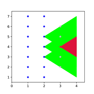
Figure 3: The x and y axes represent the time and spatial dimension, respectively. We picture the last two frames of a data set with spatial dimension $d=1$ where the blue stars represent the pixels used in the definition of the training data set, and the violet stars represent the space-time points where it is possible to provide forecasts with MMAF guided learning for $p_{t}=c=h_{t}=1$. Note that the forecast in the time-spatial position $(4,3)$ lies in the intersection (red area) of the future lightcones $A_{2}(5)^{+}$, $A_{2}(4)^{+}$ and $A_{2}(3)^{+}$ as defined in (13) and represented with green cones.

Remark 4.1.

When using the spatio-temporal embeddings described in Remark 3.9 and 3.13, similarly to the kriging literature, we need an inference step before being capable of delivering one-time ahead ensemble forecasts. In this literature, it is often assumed that the estimated parameters used in the calculation of kriging weights and kriging variances are the true one, see [23, Chapter 3] and [24, Chapter 6] for a discussion on the range of applicability of such estimates. We implicitly make the same assumptions if, for example, we use the value of the parameters $\lambda$ and $c$ in determining the parameter $a_{t}$ as suggested in Remark 3.9 and 3.13.

It remains an interesting open problem to understand the interplay of the estimates’ bias of the parameters involved in the computation of the PAC Bayesian bounds (30) and (34). One of the biggest problems of this analysis relies upon disentangling the effect of the bias of the constant $c$ introduced in the pre-processing step, which changes the length of the input-features vector $X_{i}$.

We detail now the MMAF-guided learning methodology to determine one-time ahead ensemble forecasts employing a randomized Gibbs estimator. We always consider in the procedure the estimation of the parameter $\lambda$ and $c$ because they allow us to empirically compute the right-hand side of the PAC Bayesian bound (30) or (36). Differently from the notations so far employed, we indicate the training data set by $S_{m}^{x^{*}}$ to remark the dependence of the training data set on the pixel position $x^{*}$ where we perform our forecasts.

• We choose the accuracy level $\epsilon$.

• We observe a raster data cube whose spatio-temporal index set is described by $N$ frames and we estimate the parameters $\lambda$ and $c$ (and $\bar{\alpha}$ when necessary).

• We fix a pixel position $x^{*}$ and choose a value for the hyperparameter $p_{t}$. We then choose a spatio-temporal embedding to use. Every choice is allowed as long as $m\geq 2$. We base our choice of the parameter $a_{t}$ as suggested in Remark 3.9 or 3.13 if the training data set $S_{m}^{x^{*}}$ we can obtain is feasible, i.e., $m\geq 2$ and the right-hand side of the PAC Bayesian bound (30) or (36) is not vacuous.

• We then draw $\beta$ from the randomized Gibbs estimator determined for the training data set $S_{m}^{x^{*}}$ selected in (iii). A one-time ahead forecast corresponds to the space-time point $((t_{0}+Na)+h_{t},x^{*})$ and it is given by $\langle L_{p}^{-}((t_{0}+Na)+h_{t}),\beta\rangle$. Therefore, we can make a forecast in a future time point $t=(t_{0}+Na)+h_{t}$ as long as the set $\mathcal{I}((t_{0}+Na)+h_{t},x^{*})$, as defined in (3.1.1), has cardinality $a(p,c)$.

• We perform a so-called ensemble forecast by repeating point (iv) several numbers of times. For example, in Section 4.1 experiments, we use an ensemble of $50$ one-time ahead forecasts.

For $p_{t}=1$, MMAF-guided learning can be applied to any pixel that does not belong to the frame boundary. In general, the learning methodology applies to any pixel $x^{*}$ for which $\mathcal{I}(t_{0}+ia,x^{*})\subseteq\mathbb{T}\times\mathbb{L}$ for all $i=1,\ldots,N$.

For each realization $\beta$, the prediction we obtain in $((t_{0}+Na)+h_{t},x^{*})$ lies in the intersections of the future light cones of the space-time point indices defining $L^{-}_{p}((t_{0}+Na)+h_{t},x^{*})$, see Figure 3 for an example. This means that MMAF-guided learning enables us to make forecasts in space-time points that are plausible (under the causality concept induced by the ambit sets) starting from the set of inputs we observe.

4.1 Linear predictors: an example with simulated data

We work in the hypothesis space $\mathcal{H}^{\prime}=\{h_{\beta}(X)=\beta_{0}+\beta_{1}^{T}X,\,\textrm{for}\,\,\beta:=(\beta_{0},\beta_{1})^{\top}\in B\}$, where $B\subset\mathbb{R}^{(a(p,c)+1)}$, and use the optimal spatio-temporal embedding defined in (35) for $k=1$. We use simulated observations from an STOU, i.e., a spatio-temporal short-range dependent model with exponentially decaying $\theta$-lex weakly dependent coefficients. We use a randomized Gibbs estimator to make one-time ahead ensemble forecasts. We simulate four data sets $(Z_{t}(x))_{(t,x)\in\mathbb{T}\times\mathbb{L}}$ from a zero mean STOU process by employing the diamond grid algorithm introduced in [54] for $d=1$. The time and spatial discretization steps are chosen as $h_{t}=h_{s}=0.05$ on the spatio-temporal interval $[0,100]\times[0,10]$. Therefore $\mathbb{T}=\{h_{t},\ldots,2,000h_{t}\}$ and $\mathbb{L}=\{0,\ldots,200\}$. We use the uni-dimensional frames related to the time indices $\mathbb{T}^{train}=\{0,h_{t},\ldots,1,999h_{t}\}$ to define training data sets in the following and the frame corresponding to $\mathbb{T}^{test}=\{2000h_{t}\}$ as a test set. We choose as distribution for the Lévy seed $\Lambda^{\prime}$ a normal distribution with mean $\mu=0$ and standard deviation $\sigma=0.5$, and an $NIG(\alpha,\beta,\mu,\delta)$ distribution with $\alpha=5,\beta=0,\delta=0.2$ and $\mu=0$. We use the latter distribution to test the behavior of MMAF-guided learning for different sets of heavy-tailed data. We also generate data with different mean-reverting parameters $A$ and use different seeds in generating the Lévy basis realizations. We call these data sets GAU10, GAU1A4, NIG1A4, and NIG10. For the NIG Lévy seed described above, we generate two further spatio-temporal data sets called $(Z^{i}_{t}(x))_{(t,x)\in\mathbb{T}_{i}\times\mathbb{L}}$ for $i=1,2$ on the spatio-temporal interval $[0,1,000]\times[0,10]$. We choose $h_{t}=h_{s}=0.05$, and obtain that $\mathbb{T}_{1}=\{18,000h_{t},\ldots,20,000h_{t}\}$ and $\mathbb{T}_{2}=\{0,h_{t},\ldots,20,000h_{t}\}$. For such experiments, we have the uni-dimensional frames $\mathbb{L}=\{0,\ldots,200\}$ used to determine the training data sets correspond to $\mathbb{T}_{1}^{train}=\{18,000h_{t},\ldots,19,999h_{t}\}$ and $\mathbb{T}_{2}^{train}=\{0,h_{t},\ldots,19,999h_{t}\}$, respectively. The data sets $(Z^{i}_{t}(x))_{(t,x)\in\mathbb{T}_{i}\times\mathbb{L}}$ for $i=1,2$ are generated such that the test set for both of them corresponds to the frame at time $\mathbb{T}^{\prime,test}=\{20,000h_{t}\}$. Such data sets are called NIG1, in the following. A summary scheme of the data’s characteristics is given in Table 3. The constant $c$ is set to be equal to one for all generated data sets.

Data Set	Mean Reverting Parameter	Lévy seed	Random generator seed
GAU1A4	$A=4$	Gaussian	$1$
GAU10	$A=1$	Gaussian	$10$
NIG1	$A=1$	NIG	1
NIG1A4	$A=4$	NIG	$1$
NIG10	$A=1$	NIG	$10$

Table 3: Overview on simulated data sets with $c=1$ and spatial dimension $d=1$.

We start our procedure by estimating for each data set the parameters $c$ and $\lambda$. We use the estimators $(\ref{est_stou})$ presented in Section A.3 and the plug-in estimator $(\ref{plugin})$. The true parameter $\lambda$ being equal to $\frac{1}{2}$ or $2$ for mean reverting parameter $A=1$ or $4$, respectively. The obtained results for each data set are given in Table 4. We conduct three different experiments to showcase the performance of our methodology by performing ensemble forecasts for $p=1$. We then generate $50$ one-time ahead forecasts for each pixel in $\mathbb{L}^{\prime}=\{1,\ldots,199\}$. We use as baseline model a linear model where the estimation of the parameter vector $\beta$ is performed using the ordinary least square estimator.

Data Set	$\boldsymbol{A^{*}}$	$\boldsymbol{c^{*}}$	$\boldsymbol{\lambda^{*}}$	Frames Used
GAU1A4	$3.9684$	$0.9958$	$1.9715$	$\mathbb{T}\times\mathbb{L}$
GAU10	$0.8429$	$0.9978$	$0.4196$	$\mathbb{T}\times\mathbb{L}$
NIG1	$1.0186$	$1.0018$	$0.5111$	$\mathbb{T}_{1}\times\mathbb{L}$
NIG1	$1.0186$	$1.0019$	$0.5112$	$\mathbb{T}_{2}\times\mathbb{L}$
NIG1A4	$4.0308$	$1.0076$	$2.0461$	$\mathbb{T}\times\mathbb{L}$
NIG10	$0.9728$	$1.0021$	$0.4884$	$\mathbb{T}\times\mathbb{L}$

Table 4: Estimations of parameters $A$, $c$ and $\lambda$.

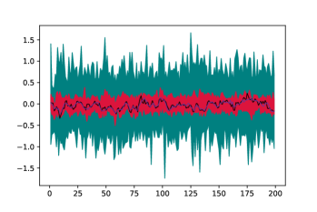
(a) GAU1A4

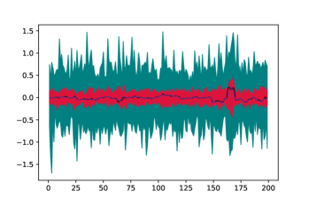
(b) NIG1A4

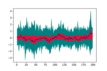
(c) GAU10

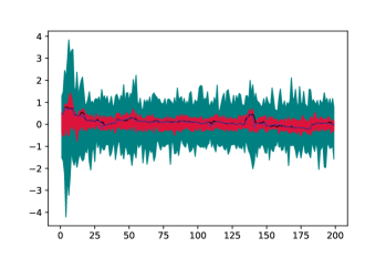
(d) NIG10

Figure 4: The x-axis represents the pixels where we perform one-time ahead forecast, whereas along the y-axis we find the forecast values. The range and inter-quartile range of an ensemble forecast of $50$ draws are, respectively, represented in green and red. The test set and the forecasts obtained by ordinary least square estimation are respectively depicted with black and viola thick lines.

In the first experiment, we use the data sets GAU1A4, GAU10, NIG1A4, NIG10 and determine the spatio-temporal embeddings described in Table 5. In our experiments, $a(p,c)=3$. We then test the performance of the randomized Gibbs estimator with convergence rate $\mathcal{O}(m^{\frac{1}{2}})$ considering as reference distribution a multivariate standard Gaussian.

GAU1A4		GAU10		NIG1A4		NIG10
a	81	a	306	a	79	a	266
m	25	m	7	m	25	m	8
k	1	k	1	k	1	k	1

Table 5: Parameters defined the training data sets $S^{x^{*}}_{m}$ for each pixel.

An acceptance-rejection algorithm with a Gaussian proposal determines a draw $\beta$. We show in Figure 4 the range and inter-quartile range of $50$ forecasts for each pixel, compared with the test set. As the plots clearly show, using a randomized Gibbs estimator, we obtain an inter-quartile range containing the test set for each spatial position $x^{*}\in\mathbb{L}^{\prime}$. To compare our forecasts with the baseline model, let us define the average Relative Root Mean Squared Error (averRMSE) as follows. Let $P=|\mathbb{L}^{\prime}|$, we define the average Relative Mean Squared Error as

$$\textit{aver}RMSE=\sqrt{\frac{\frac{1}{P}\sum_{i=1}^{P}(Z_{t}(x_{i})-\hat{Z}_{t}(x_{i}))^{2}}{\sum_{i=1}^{P}\hat{Z}_{t}(x_{i})^{2}}},$$

where $\hat{Z}_{t}(x_{i})$ is the one-time ahead forecast obtained with the linear model for all $i$. Our data sets’ observations have an order of magnitude (on average) of $10^{-3}$. Table 6 states that the least square estimator cannot capture any significant digit, as also seen in Figure 4. Our ensemble forecasts give, at least, an interval where the one-time ahead forecasts can lie.

	GAU1A4	GAU10	NIG1A4	NIG10	NIG1
linear	$0.0027$	$0.0032$	$0.0101$	$0.0037$	$0.0051$

Table 6: averRMSE for the linear model forecasts.

In the second experiment, we observe the performance of the Gibbs estimator for the data sets NIG1. We use the same algorithm and spatio-temporal embedding as in the first experiment. Therefore, for each pixel, we work with the two training data sets $S^{1,x^{*}}_{m}$ and $S^{2,x^{*}}_{m}$ described in Table 7 and obtain the ensemble forecasts in Figure 5.

NIG1
$S^{1,x^{*}}_{m}$		$S^{2,x^{*}}_{m}$
a	255	a	255
m	8	m	78
k	1	k	1

Table 7: Parameters describing the training data sets used in the second experiment at each pixel position $x^{*}$.

We compare the inter-quartile range of the ensemble forecasts, and we see that the green range, representing the forecasts related to $S^{2,x^{*}}_{m}$, is contained in the purple range, representing the ones obtained using $S^{1,x^{*}}_{m}$. Both of them include the test set. The amplitude of the inter-quartile range reduces when the number of observations in the training data set increases. The forecasts of the baseline model are performed using the training data set $S^{2,x^{*}}_{m}$ and have a high averRMS as reported in Table 6.

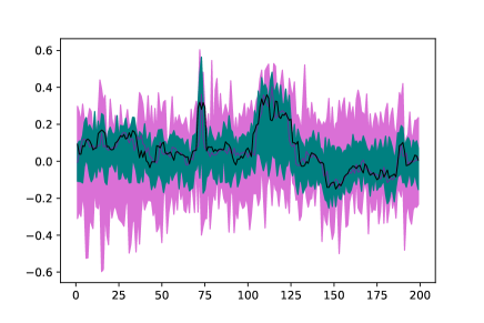
Figure 5: Inter-quartile range of 50 one-time ahead forecasts using the training data sets $S^{1,x^{*}}_{m}$ (in violet) and $S^{2,x^{*}}_{m}$ (in green) for each pixel $x^{*}$. The test set and the forecasts obtained with ordinary least square estimation using the data set $\mathbb{T}_{2}^{train}$ are respectively depicted with black and violet thick lines. The x-axis represents the pixels where we perform the one-time ahead forecast.

We want now to analyze the sensitivity of our methodology to the choice of the hyperparameters $\epsilon$ and $p_{t}$ when $a_{t}$ is selected following (35). The selection of the parameter $a_{t}$ is proportional to the values of both parameters. Therefore, the smaller we choose them, the higher is the number of examples we obtain in $S^{x^{*}}_{m}$. We work in this experiment with the data sets GAU1A4 and NIG1A4. However, we obtain the same conclusions for all the other data sets employed in our experiments.

We generate ensemble forecasts (and their respective inter-quartile ranges) for $p=1,2,3$. All inter-quartile ranges contain the test set and their amplitude has minimal differences. For this reason, in our previous experiments we have chosen the parameter $p_{t}=1$.

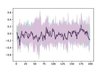
(a) GAU1A4

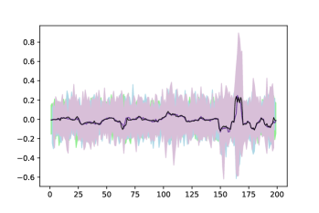
(b) NIG1A4

Figure 6: Inter-quantile range for $p=1$ (green), $p=2$ (blue), $p=3$ (lilac). The test set and the forecasts obtained by ordinary least square estimation, respectively depicted in black and violet thick lines. The x-axis represents the pixels where we perform the one-time ahead forecast.

(a) GAU1A4

(b) NIG1A4

Figure 7: Inter-quantile range for $\epsilon=2$ (green), $\epsilon=3$ (gold), $\epsilon=4$ (maroon). The test set and the forecasts obtained by ordinary least square estimation, respectively depicted in black and viola thick lines. The x-axis represents the pixels where we perform the one-time ahead forecast.

Let us now perform ensemble forecasts for $\epsilon=2,3,4$. We notice a clear reduction of the size of the inter-quartile range for smaller $\epsilon$. We chose in our experiment $\epsilon=3$ because it performs in between the scenario we consider in the sensitivity analysis and allows a milder cut-off of the loss function.

5 Conclusions

We define a novel theory-guided machine learning methodology for spatio-temporal data. In particular, our methodology applies to raster data cubes. We choose as the data generating process an influenced mixed moving average field defined on a cone-shaped ambit set. Such a step requires the specification of a kernel function, which includes the presence of a random parameter (if spatial and temporal long-range dependence is desired), a Lévy seed with finite second-order moments, and the speed of information propagation constant. The latter determines the width of the ambit sets.

To enable one-time ahead ensemble forecasts, we use the underlying model to define a spatio-temporal embedding that preserves the dependence structure of the latter and reduces the number of past and neighboring space-time points used in the learning phase as much as possible. MMAF-guided learning applies to the class of Lipschitz function, which includes linear functions and several types of neural network modules, and utilizes a generalized Bayesian algorithm to perform one-time ahead ensemble forecasts. We show different types of PAC Bayesian bounds in the paper to describe the range of applicability of our methodology in the function of different spatio-temporal embeddings. A randomized Gibbs estimator minimizes the PAC Bayesian bounds derived in the paper.

In conclusion, we test the learning procedure for a randomized Gibbs estimator for a Gaussian reference distribution that has a convergence rate of $\mathcal{O}(m^{\frac{1}{2}})$ on the class of linear models. We simulate a set of six simulated data sets from an STOU process with Gaussian and NIG Lévy seed and determine ensemble forecasts. We obtain that the inter-quartile range of our forecasts contains the test set and shrinks when the cardinality of the training data set increases. Moreover, our forecasts have a causal interpretation induced by the ambit sets employed in the data generating process. The concept of causality employed in the paper can be inscribed in the potential outcomes framework.

Appendix A

A.1 Weak dependence notions for causal processes and (influenced) MMAF

In this section, we discuss more in details the asymptotic independence notions called $\theta$-weak dependence and $\theta$-lex weak dependence. The latter notion has been introduced in [26, Definition 2.1] as an extension to the random field case of the notion of $\theta$-weak dependence satisfied by causal stochastic processes [29]. This notion of dependence is presented in Definition 2.14. However, the notion of $\theta$-lex weak dependence given in Definition 2.13 slightly differs from the one given in [26, Definition 2.1] and represents an extension to the random field case of the $\theta$-weak dependence notion defined in [30, Remark 2.1]. Note that the definitions of $\theta$-weak dependence in [29] and [30, Remark 2.1] differ because of the cardinality of the marginal distributions on which the function $G$ is computed, namely, $G\in\mathcal{G}_{1}$ in the former and $G\in\mathcal{G}_{\nu}$ for $\nu\in\mathbb{N}$ in the latter.

Remark A.1 (Mixingale-type representation of $\theta$-weak dependence).

Let $\mathcal{L}_{1}=\{g:\mathbb{R}\to\mathbb{R},\,\text{bounded and}$ $\textrm{Lipschitz continuous with}\,\,Lip(g)\leq 1\}$, a stochastic process $(\boldsymbol{X}_{t})_{t\in\mathbb{Z}}$, and $\mathcal{M}=\sigma\{\boldsymbol{X}_{t}:t<j_{1},t\in\mathbb{Z}\}$, then it is showed in [30, Proposition 2.3] that

$$\theta(r)=\sup_{g\in\mathcal{L}_{1}}\|\mathbb{E}[g(\boldsymbol{X}_{j_{1}})|\mathcal{M}]-\mathbb{E}[g(\boldsymbol{X}_{j_{1}})]\|_{1}.$$ (39)

An alternative proof of this result can be also found in [29, Lemma 1].

Let us now analyze the relationship between $\theta$-weak dependence, $\alpha$-mixing, and $\phi$-mixing. Most of the PAC Bayesian literature for stationary and heavy tailed data employs the following two mixing conditions, see Remark 3.19, namely $\alpha$-mixing and $\phi$-mixing. The results in the Lemma below give us a proof that the $\theta$-weak dependence is more general than $\alpha$-mixing and $\phi$-mixing and therefore describes the dependence structure of a bigger class of models.

Let $\mathcal{M}$ and $\mathcal{V}$ be two sub-sigma algebras of $\mathcal{F}$. First of all, the strong mixing coefficient [65] is defined as

$$\alpha(\mathcal{M},\mathcal{V})=\sup\{|P(M)P(V)-P(M\cap V)|,M\in\mathcal{M},V\in\mathcal{V}\}.$$

A stochastic process $\boldsymbol{X}$ is said to be $\alpha$-mixing if

$$\alpha(r)=\alpha(\sigma\{\boldsymbol{X}_{s},s\leq 0\},\sigma\{\boldsymbol{X}_{s},s\geq r\})$$

converges to zero as $r\to\infty$. The $\phi$-mixing coefficient has been introduced in [45] and defined as

$$\phi(\mathcal{M},\mathcal{V})=\sup\{|P(V|M)-P(V)|,M\in\mathcal{M},V\in\mathcal{V},P(M)>0\}.$$

A stochastic process $\boldsymbol{X}$ is said to be $\phi$-mixing if

$$\phi(r)=\phi(\sigma\{\boldsymbol{X}_{s},s\leq 0\},\sigma\{\boldsymbol{X}_{s},s\geq r\})$$

converges to zero as $r\to\infty$.

Lemma A.2.

Let $(\boldsymbol{X}_{t})_{t\in\mathbb{Z}}$ be a stationary real-valued stochastic process such that $\mathbb{E}[|\boldsymbol{X}_{0}|^{q}]<\infty$ for some $q>1$. Then,

• $\theta(r)\leq 2^{\frac{2q-1}{q}}\alpha(r)^{\frac{q-1}{q}}\|\boldsymbol{X}_{0}\|_{q}\leq 2^{\frac{q-1}{q}}\phi(r)^{\frac{q-1}{q}}\|\boldsymbol{X}_{0}\|_{q}$, and

• $\theta$-weak dependence is a more general dependence notion than $\alpha$-mixing and $\phi$-mixing.

Proof.

The proof of the first inequality at point (a) is proven in [26, Proposition 2.5] using the representation of the $\theta$-coefficients (39). The proof of the second inequality follows from a classical result in [18, Proposition 3.11]. In [26, Proposition 2.7], it is defined a stochastic process which is $\theta$-weak dependent but neither $\alpha$-mixing or $\phi$-mixing.    

As seen in Definition 2.13 by using the lexicographic order in $\mathbb{R}^{1+d}$, an opportune extension of $\theta$-weak dependence valid for random fields can be defined.

The definition of $\theta$-lex coefficients for $G\in\mathcal{G}_{1}$ is given in [26, Definition 2.1]. The latter can be represented as $\theta_{lex}^{v}(r):=\sup_{u\in\mathbb{N}}\{\theta_{u,v}(r)\}$ for $v=1$. Therefore, an alternative way to define the $\theta$-lex coefficients in Definition 2.13 is obviously

$$\theta_{lex}(r)=\sup_{v\in\mathbb{N}}\theta_{lex}^{v}(r),v\in\mathbb{N}\,\,\,\textrm{for all $r\in\mathbb{R}^{+}$.}$$ (40)

The following Lemma has important applications in the following sections.

Lemma A.3.

Let $\boldsymbol{Z}$ be a $\theta$-lex weakly dependent random field, then $\boldsymbol{Z}_{i}^{M}=\boldsymbol{Z}_{i}\vee(-M)\wedge M$ is $\theta$-lex weakly dependent.

Proof.

Let $u,v\in\mathbb{N}$, $M>0$, $F\in\mathcal{G}^{*}_{u}$, $G\in\mathcal{G}_{v}$, and $i_{1},i_{2},\ldots,i_{u}\in V_{\Gamma^{\prime}}^{r}$ where $\Gamma^{\prime}=\{j_{1},\ldots,j_{v}\}$. Let $F^{M}(\boldsymbol{Z}_{i_{1}},\ldots,\boldsymbol{Z}_{i_{u}})=F(\boldsymbol{Z}_{i_{1}}^{M},\ldots,\boldsymbol{Z}_{i_{u}}^{M})$, and $G^{M}(\boldsymbol{Z}_{j_{1}},\ldots,\boldsymbol{Z}_{j_{v}})=G(\boldsymbol{Z}_{j_{1}}^{M},\ldots,\boldsymbol{Z}_{j_{v}}^{M})$. We have that $F^{M}$ is a bounded function on $(\mathbb{R}^{n})^{u}$ and $G^{M}$ is a bounded and Lipschitz function on $(\mathbb{R}^{n})^{v}$ (with the same Lipschitz coefficients as the function $G$). Let $(\boldsymbol{Z}_{1},\ldots,\boldsymbol{Z}_{v})$ and $(\tilde{\boldsymbol{Z}}_{1},\ldots,\tilde{\boldsymbol{Z}}_{v})\in(\mathbb{R}^{n})^{v}$, then

$$|G^{M}(\boldsymbol{Z}_{1},\ldots,\boldsymbol{Z}_{v})-G^{M}(\tilde{\boldsymbol{Z}}_{1},\ldots,\tilde{\boldsymbol{Z}}_{v})|\leq Lip(G)\sum_{i=1}^{v}|\boldsymbol{Z}_{i}^{M}-\tilde{\boldsymbol{Z}}_{i}^{M}|$$

$$\leq Lip(G)\sum_{i=1}^{v}|\boldsymbol{Z}_{i}-\tilde{\boldsymbol{Z}}_{i}|.$$

Hence, it holds that

$$|Cov(F(\boldsymbol{Z}_{i_{1}}^{M},\ldots,\boldsymbol{Z}_{i_{u}}^{M}),G(\boldsymbol{Z}_{j_{1}}^{M},\ldots,\boldsymbol{Z}_{j_{v}}^{M}))|\leq\|F\|_{\infty}vLip(G)\theta_{lex}(r),$$

where $\theta_{lex}(r)$ are the $\theta$-coefficients of the field $\boldsymbol{Z}$, and so the field $\boldsymbol{Z}_{t}^{M}(x)$ is $\theta$-lex weakly dependent.    

Note that the above result also holds for $\boldsymbol{X}$ a $\theta$-weakly dependent process. Therefore, the truncated $\boldsymbol{X}_{t}^{M}=\boldsymbol{X}_{t}\vee(-M)\wedge M$ is a $\theta$-weakly dependent process.

The notion of $\theta$-lex weak dependence also admits a mixingale-type representation.

Remark A.4.

Let $\mathcal{L}_{1}=\{g:\mathbb{R}\to\mathbb{R},\,\text{bounded and Lipschitz continuous with}\,\,Lip(g)\leq 1\}$ and $\Gamma^{\prime}=\{j_{1},\ldots,j_{v}\}$ for $\{j_{1},\ldots j_{v}\}\in\mathbb{Z}^{1+d}$. For a random field $(\boldsymbol{Z}_{t})_{t\in\mathbb{Z}^{1+d}}$, by readily applying [26, Lemma 5.1] on the $\sigma$-algebra $\mathcal{M}=\sigma\{\boldsymbol{Z}_{t}:t\in V^{r}_{\Gamma^{\prime}}\subset\mathbb{Z}^{1+d}\}$, the following result can be easily proved:

$$\theta_{lex}(r)=\sup_{g\in\mathcal{L}_{1}}\sup_{v\in\mathbb{N}}\|\mathbb{E}[g(\boldsymbol{Z}_{j_{1}},\ldots,\boldsymbol{Z}_{j_{v}})|\mathcal{M}]-\mathbb{E}[g(\boldsymbol{Z}_{j_{1}},\ldots,\boldsymbol{Z}_{j_{v}})]\|_{1}.$$ (41)

We now use the representation of the $\theta$-lex coefficients (41) to understand its relationships to $\alpha_{\infty,v}$-mixing and $\phi_{\infty,v}$-mixing for $v\in\mathbb{N}\cup\{\infty\}$. These notions are defined in [28] and they are strong mixing notions used in the study of stationary random fields.

In general, for $u,v\in\mathbb{N}\cup\{\infty\}$, given coefficients

$$\alpha_{u,v}(r)=\sup\{\alpha(\sigma(\boldsymbol{Z}_{\Gamma}),\sigma(\boldsymbol{Z}_{\Gamma^{\prime}})),\Gamma,\Gamma^{\prime}\in\mathbb{R}^{1+d},|\Gamma|\leq u,|\Gamma^{\prime}|\leq v,dist(\Gamma,\Gamma^{\prime})\geq r\},$$

and

$$\phi_{u,v}(r)=\sup\{\phi(\sigma(\boldsymbol{Z}_{\Gamma}),\sigma(\boldsymbol{Z}_{\Gamma^{\prime}})),\Gamma,\Gamma^{\prime}\in\mathbb{R}^{1+d},|\Gamma|\leq u,|\Gamma^{\prime}|\leq v,dist(\Gamma,\Gamma^{\prime})\geq r\}.$$

a random field $\boldsymbol{Z}$ is said to be $\alpha_{u,v}$-mixing or $\phi_{u,v}$-mixing if the coefficients $(\alpha_{u,v}(r))_{r\in\mathbb{R}^{+}}$ or $(\phi_{u,v}(r))_{r\in\mathbb{R}^{+}}$ converge to zero as $r\to\infty$. We then have the following result.

Lemma A.5.

Let $(\boldsymbol{Z}_{t})_{t\in\mathbb{Z}^{1+d}}$ be a stationary real-valued random field such that $\mathbb{E}[|\boldsymbol{Z}_{0}|^{q}]<\infty$ for some $q>1$. Then, for $v\in\mathbb{N}\cup\{\infty\}$,

• $\theta_{lex}(r)\leq 2^{\frac{2q-1}{q}}\alpha_{\infty,v}(r)^{\frac{q-1}{q}}\|\boldsymbol{Z}_{0}\|_{q}\leq 2^{\frac{q-1}{q}}\phi_{\infty,v}(r)^{\frac{q-1}{q}}\|\boldsymbol{Z}_{0}\|_{q}$, and

• it holds that $\theta$-lex weak dependence is more general than $\alpha_{\infty,v}$-mixing and $\alpha$-mixing in the special case of stochastic processes. Moreover, $\theta$-lex weak dependence is more general than $\phi_{\infty,v}$-mixing.

Proof.

From the proof of [26, Proposition 2.5], we have that

$$\theta_{lex}^{1}(r)\leq 2^{\frac{2q-1}{q}}\alpha_{\infty,1}(r)^{\frac{q-1}{q}}\|\boldsymbol{Z}_{0}\|_{q}.$$

Because of (40) and [18, Proposition 3.11], we have that

$$\theta_{lex}(r)\leq 2^{\frac{2q-1}{q}}\alpha_{\infty,1}(r)^{\frac{q-1}{q}}\|\boldsymbol{Z}_{0}\|_{q}\leq 2^{\frac{q-1}{q}}\phi_{\infty,1}(r)^{\frac{q-1}{q}}\|\boldsymbol{Z}_{0}\|_{q}.$$

Equally,

$$\theta_{lex}(r)\leq 2^{\frac{2q-1}{q}}\alpha_{\infty,v}(r)^{\frac{q-1}{q}}\|\boldsymbol{Z}_{0}\|_{q}\leq 2^{\frac{q-1}{q}}\phi_{\infty,v}(r)^{\frac{q-1}{q}}\|\boldsymbol{Z}_{0}\|_{q}.$$

The proof of the point (b) follows directly by [26, Proposition 2.7]. In fact $\theta_{lex}(r)=\theta_{1,\infty}(r)$ following the notations of [30, Definition 2.3] and the process used in the proof of the Proposition is $\theta$-lex weakly dependent but neither $\alpha_{\infty,v}$, $\alpha$ or $\phi_{\infty,v}$-mixing.

   

A.2 Autocovariance Structure of MMAF and Isotropy

Moment conditions for MMAFs are typically expressed in function of the characteristic quadruplet of its driving Lévy basis and the kernel function $f$.

Proposition A.6.

Let $\boldsymbol{Z}$ be an $\mathbb{R}$-valued MMAF driven by a Lévy basis with characteristic quadruplet $(\gamma,\sigma^{2},\nu,\pi)$ with kernel function $f:H\times\mathbb{R}\times\mathbb{R}^{d}\rightarrow\mathbb{R}$ and defined on an ambit set $A_{t}(x)\subset\mathbb{R}\times\mathbb{R}^{d}$.

1. If $\int_{|x|>1}|x|\nu(dx)<\infty$ and $f\in L^{1}(H\times\mathbb{R}\times\mathbb{R}^{d})\cap L^{2}(H\times\mathbb{R}\times\mathbb{R}^{d})$ the first moment of $\boldsymbol{Z}$ is given by

   $$\mathbb{E}[\boldsymbol{Z}_{t}]=\mathbb{E}(\Lambda^{\prime})\int_{H}\int_{A_{t}(x)}f(A,-s,-\xi)ds\,d\xi\,\pi(dA),$$

   where $\mathbb{E}(\Lambda^{\prime})=\gamma+\int_{|x|\geq 1}x\,\nu(dx)$.

2. If $\int_{\mathbb{R}}x^{2}\,\nu(dx)<\infty$ and $f\in L^{2}(H\times\mathbb{R}\times\mathbb{R}^{d})$, then $\boldsymbol{Z}\in L^{2}(\Omega)$ and

   $$Var(\boldsymbol{Z}_{t}(x))=Var(\Lambda^{\prime})\int_{H}\int_{\mathbb{R}\times\mathbb{R}^{d}}f(A,-s,-\xi)^{2}ds\,d\xi\,\pi(dA),$$

   $$Cov(\boldsymbol{Z}_{0}(0),\boldsymbol{Z}_{t}(x))=Var(\Lambda^{\prime})\int_{H}\int_{A_{0}(0)\cap A_{t}(x)}f(A,-s,-\xi)f(A,t-s,x-\xi)\,ds\,d\xi\,\pi(dA)\hskip 14.22636pt\text{and}$$

   $$Corr(\boldsymbol{Z}_{0}(0),\boldsymbol{Z}_{t}(x))=\frac{\int_{H}\int_{A_{0}(0)\cap A_{t}(x)}f(A,-s,-\xi)f(A,t-s,x-\xi)\,ds\,d\xi\,\pi(dA)}{\int_{H}\int_{\mathbb{R}\times\mathbb{R}^{d}}f(A,-s,-\xi)^{2}ds\,d\xi\,\pi(dA)},$$ (42)

   where $Var(\Lambda^{\prime})=\sigma^{2}+\int_{\mathbb{R}^{d}}xx^{\prime}\nu(dx)$.

3. If $\sigma^{2}=0$, $\int_{|x|\in\mathbb{R}}|x|\,\nu(dx)<\infty$, and $f\in L^{1}(H\times\mathbb{R}\times\mathbb{R}^{d})$, then the first moment of $\boldsymbol{Z}$ is given by

   $$E[\boldsymbol{Z}_{t}(x)]=\int_{H}\int_{A_{t}(x)}f(A,-s,-\xi)\Big{(}\gamma_{0}+\int_{\mathbb{R}}x\nu(dx)\Big{)}ds\,d\xi\,\pi(dA),$$

   where

   $$\gamma_{0}:=\gamma-\int_{|x|\leq 1}x\,\nu(dx).$$ (43)

Proof.

Immediate from [68, Section 25] and [26, Theorem 3.3].    

From Proposition A.6, we can evince that the autocovariance function of an MMAF depends on the variance of the Lévy seed $\Lambda^{\prime}$, the kernel function $f$ and the distribution $\pi$ of the random parameter $A$.

We give below the explicit expression of the autocovariance functions for an STOU and MSTOU process.

Example A.7.

Let $\boldsymbol{Z}$ ad defined in Example 2.8, $u\in\mathbb{R}^{d}$, $\tau\in\mathbb{R}$, and $\mathbb{E}[\boldsymbol{Z}_{t}(x)^{2}]<\infty$. Then,

$$Cov(\boldsymbol{Z}_{t}(x),\boldsymbol{Z}_{t+\tau}(x+u))=Var(\Lambda^{\prime})\exp(-A\tau)\int_{A_{t}(x)\cap A_{t+\tau}(x+u)}\exp(-2A(t-s))ds\,d\xi,\,\,\,\textrm{and}$$ (44)

$$Corr(\boldsymbol{Z}_{t}(x),\boldsymbol{Z}_{t+\tau}(x+u))=\frac{\exp(-A\tau)\int_{A_{t}(x)\cap A_{t+\tau}(x+u)}\exp(-2A(t-s))\,\,ds\,d\xi}{\int_{A_{t}(x)}\exp(-2A(t-s))\,\,ds\,d\xi}.$$ (45)

Example A.8.

Let $\boldsymbol{Z}$ ad defined in Example 2.8 and $d=1$, then

$$\rho^{T}(\tau):=Corr(\boldsymbol{Z}_{t}(x),\boldsymbol{Z}_{t+\tau}(x))=\exp(-A|\tau|),$$ (46)

$$\rho^{S}(u):=Corr(\boldsymbol{Z}_{t}(x),\boldsymbol{Z}_{t}(x+u))=\exp\Big{(}-A\frac{|u|}{c}\Big{)},$$ (47)

$$\rho^{ST}(\tau,u):=Corr(\boldsymbol{Z}_{t}(x),\boldsymbol{Z}_{t+\tau}(x+u))=\min\Big{(}\exp(-A|\tau|),\exp\Big{(}-\frac{A|u|}{c}\Big{)}\Big{)}.$$ (48)

Example A.9.

Let $\boldsymbol{Z}$ be defined as in Example 2.9, $u\in\mathbb{R}^{d}$ and $\tau\in\mathbb{R}$, and $\mathbb{E}[\boldsymbol{Z}_{t}(x)^{2}]<\infty$, then

$$Cov(\boldsymbol{Z}_{t}(x),\boldsymbol{Z}_{t+\tau}(x+u))=Var(\Lambda^{\prime})\exp(-A\tau)\int_{0}^{\infty}\int_{A_{t}(x)\cap A_{t+\tau}(x+u)}\exp(-2A(t-s))ds\,d\xi\,l(A)dA,$$ (49)

$$Corr(\boldsymbol{Z}_{t}(x),\boldsymbol{Z}_{t+\tau}(x+u))=\frac{\exp(-A\tau)\int_{0}^{\infty}\int_{A_{t}(x)\cap A_{t+\tau}(x+u)}\exp(-2A(t-s))\,\,ds\,d\xi\,l(A)dA}{\int_{0}^{\infty}\int_{A_{t}(x)}\exp(-2A(t-s))\,\,ds\,d\xi\,l(A)dA}.$$ (50)

Example A.10.

Let $\boldsymbol{Z}$ be defined as in Example 2.9 for $d=1$, Assumption 2.10 hold, and $l(A)=\frac{\beta^{\alpha}}{\Gamma(\alpha)}A^{\alpha-1}\exp(-\beta A)$ be the Gamma density with shape and rate parameters $\alpha>d+1$ and $\beta>0$. For $d=1$, $u\in\mathbb{R}$ and $\tau\in\mathbb{R}$

$$Var(\boldsymbol{Z}_{t}(x))=\frac{Var(\Lambda^{\prime})c\beta^{2}}{2(\alpha-2)(\alpha-1)}$$ (51)

$$Cov(\boldsymbol{Z}_{t}(x),\boldsymbol{Z}_{t+\tau}(x+u))=\frac{Var(\Lambda^{\prime})c\beta^{\alpha}}{2(\beta+\max\{|\tau|,|u|/c\})^{\alpha-2}(\alpha-2)(\alpha-1)},$$ (52)

$$\rho^{ST}(\tau,u):=Corr(\boldsymbol{Z}_{t}(x),\boldsymbol{Z}_{t+\tau}(x+u))=\Bigg{(}\frac{\beta}{\beta+\max\{|\tau|,|u|/c\}}\Bigg{)}^{\alpha-2}.$$ (53)

It follows the definition of an isotropic spatio-temporal random field.

Definition A.11 (Isotropy).

Let $t\in\mathbb{R}$ and $x\in\mathbb{R}^{d}$. A spatio-temporal random field $(\boldsymbol{Z}_{t}(x))_{(t,x)\in\mathbb{R}\times\mathbb{R}^{d}}$ is called isotropic if its spatial covariance:

$$Cov(\boldsymbol{Z}_{t}(x),\boldsymbol{Z}_{t}(x+u))=C(|u|),$$

for some positive definite function $C$.

STOU and MSTOU processes defined on cone-shaped ambit sets are isotropic random fields.

A.3 Inference on STOU processes

Let us start by explaining the available estimation methodologies for the parameter vector $\theta_{0}=\{A,c,Var(\Lambda^{\prime})\}$ under the STOU modeling assumption when the spatial dimension $d=1$. Throughout, we refer to the notations used in Example 2.18.

We have two ways of estimating the parameter vector $\theta_{0}$ in such a scenario. The first one is presented in [54]. Here, the parameters $A$ and $c$ are first estimated using normalized spatial and temporal variograms defined as

$$\gamma^{S}(u):=\frac{\mathbb{E}((\boldsymbol{Z}_{t}(x)-\boldsymbol{Z}_{t}(x-u))^{2})}{Var(\boldsymbol{Z}_{t}(x))}=2(1-\rho^{S}(u))=2\Big{(}1-\exp\Big{(}-\frac{Au}{c}\Big{)}\Big{)},$$ (54)

and

$$\gamma^{T}(\tau):=\frac{\mathbb{E}((\boldsymbol{Z}_{t}(x)-\boldsymbol{Z}_{t-\tau}(x))^{2})}{Var(\boldsymbol{Z}_{t}(x))}=2(1-\rho^{T}(\tau))=2(1-\exp(-A\tau)),$$ (55)

where $\rho^{S}$ and $\rho^{T}$ are defined in Example A.8. Note that normalized variograms are used to separate the estimation of the parameters $A$ and $c$ from the parameter $Var(\Lambda^{\prime})$. Let $N(u)$ be the set containing all the pairs of indices at mutual spatial distance $u$ for $u>0$ and the same observation time. Let $N(\tau)$ be the set containing all the pairs of indices where the observation times are at a distance $\tau>0$ and have the same spatial position. $|N(u)|$ and $|N(\tau)|$ give the number of the obtained pairs, respectively. Moreover, let $\boldsymbol{\hat{k}}_{2}$ be the empirical variance which is defined as

$$\boldsymbol{\hat{k}}_{2}=\frac{1}{(D-1)}\sum_{i=1}^{D}\boldsymbol{Z^{2}}_{t_{i}}(x_{i}),$$ (56)

where $D$ denotes the sample size. The empirical normalized spatial and temporal variograms are then defined as follows:

$$\boldsymbol{\hat{\gamma}}^{S}(u)=\frac{1}{|N(u)|}\sum_{i,j\in N(u)}\frac{(\boldsymbol{Z}_{t_{i}}(x_{i})-\boldsymbol{Z}_{t_{j}}(x_{j}))^{2}}{\boldsymbol{\hat{k}_{2}}}$$ (57)

$$\boldsymbol{\hat{\gamma}}^{T}(\tau)=\frac{1}{|N(\tau)|}\sum_{i,j\in N(\tau)}\frac{(\boldsymbol{Z}_{t_{i}}(x_{i})-\boldsymbol{Z}_{t_{j}}(x_{j}))^{2}}{\boldsymbol{\hat{k}_{2}}}.$$ (58)

By matching the empirical and the theoretical forms of the normalized variograms, we can estimate $A$ and $c$ by employing the estimators

$$\boldsymbol{A^{*}}=-\tau^{-1}\log\Big{(}1-\frac{\boldsymbol{\hat{\gamma}^{T}}(\tau)}{2}\Big{)},\,\,\,\textrm{and}\,\,\,\boldsymbol{c^{*}}=-\frac{\boldsymbol{A^{*}}u}{\log\Big{(}1-\frac{\boldsymbol{\hat{\gamma}^{S}}(u)}{2}\Big{)}}.$$ (59)

Alternatively, we can use a least square methodology to estimate the parameters $A$ and $c$, i.e. (57) and (58) are computed at several lags, and a least-squares estimation is used to fit the computed values to the theoretical curves. The authors in [54] use the methodology discussed in [50] to achieve the last target. We refer the reader also to [23, Chapter 2] for further discussions and examples of possible variogram model fitting. The parameter $Var(\Lambda^{\prime})$ can be estimated by matching the second-order cumulant of the STOU with its empirical counterpart. The consistency of this estimation procedure is proven in [54, Theorem 12].

A second possible methodology for estimating the vector $\theta_{0}$ employs a generalized method of moment estimator (GMM), as in [55]. It is essential to notice that by using such an estimator, we cannot separate the parameter $Var(\Lambda^{\prime})$ from the estimation of the parameters $A$ and $c$. Instead, all moment conditions must be combined into one optimization criterion, and all the estimations must be found simultaneously. Consistency and asymptotic normality of the GMM estimator are discussed in [55] and [26], respectively.

For $d\geq 2$, a least square methodology is still applicable for estimating the variogram’s parameters. The estimator used in [54] is a normalized version of the least-square estimator for spatial variogram’s parameters discussed in [50], which also applies for $d>1$. This method, paired with a method of moments (matching the second order cumulant of the field $\boldsymbol{Z}$ with its empirical counterparts), allows estimating the parameter $Var(\Lambda^{\prime})$. The GMM methodology discussed in [55] also continues to apply for $d\geq 2$. However, when the spatial dimension is increasing, the shape of the normalized variograms and the field’s moments become more complex, and higher computational effort is required to navigate through the high dimensional surface of the optimization criterion behind least-squares or GMM estimators.

A.4 Inference for MSTOU processes

When estimating the parameter vector $\theta_{1}=\{\alpha,\beta,c,Var(\Lambda^{\prime})\}$ under an MSTOU modeling assumption– see, for example, solely the shape of the coefficients in Example 2.19– it is evident that the shape of the autocorrelation function, and therefore of the normalized temporal and spatial variograms, become more complex for increasing $d$. As already addressed in the previous sections, when estimating the parameters $(\alpha,\beta,c)$ alone, we can use the least-squares type estimator discussed in [50]. Moreover, by pairing the latter with a method of moments or using a GMM estimator, we can estimate the complete vector $\theta_{1}$.

A.5 Time series models

In the MMAF framework, we can also find time series models. The latter are $\theta$-weakly dependent.

Example A.12 (Time series case).

The supOU process studied in [7] and [12] is an example of a causal mixed moving average process. Let the kernel function $f(A,s)=\mathrm{e}^{-As}1_{[0,\infty)}(s)$, $A\in\mathbb{R}^{+}$, $s\in\mathbb{R}$ and $\Lambda$ a Lévy basis on $\mathbb{R}^{+}\times\mathbb{R}$ with generating quadruple $(\gamma,\sigma^{2},\nu,\pi)$ such that

$$\int_{|x|>1}\log(|x|)\,\nu(dx)<\infty,\,\,\textrm{and}\,\,\int_{\mathbb{R}^{+}}\frac{1}{A}\pi(dA)<\infty,$$ (60)

then the process

$$\boldsymbol{Z}_{t}=\int_{\mathbb{R}^{+}}\int_{-\infty}^{t}\mathrm{e}^{-A(t-s)}\,\Lambda(dA,ds)$$ (61)

is well defined for each $t\in\mathbb{R}$ and strictly stationary and called a supOU process where $A$ represents a random mean reversion parameter.

If $\mathbb{E}(\Lambda^{\prime})=0$ and $\int_{|x|>1}|x|^{2}\nu(dx)<\infty$, the supOU process is $\theta$-weakly dependent with coefficients

$$\theta_{Z}(r)\leq\Big{(}\int_{\mathbb{R}^{+}}\int_{-\infty}^{r}\mathrm{e}^{-2As}\sigma^{2}\,ds\,\pi(dA)\Big{)}^{\frac{1}{2}}=\Big{[}Var(\Lambda^{\prime})\int_{\mathbb{R}^{+}}\frac{\mathrm{e}^{-2Ar}}{2A}\,\pi(dA)\Big{]}^{\frac{1}{2}}$$ (62)

$$=Cov(\boldsymbol{Z}_{0},\boldsymbol{Z}_{2r})^{\frac{1}{2}},$$

where $Var(\Lambda^{\prime})=\sigma^{2}+\int_{\mathbb{R}}x^{2}\nu(dx)$, by using Theorem 3.11 in [12].

If $\mathbb{E}(\Lambda^{\prime})=\mu$ and $\int_{|x|>1}|x|^{2}\nu(dx)<\infty$, the supOU process is $\theta$-weakly dependent with coefficients

$$\theta_{Z}(r)\leq\Big{(}Cov(\boldsymbol{Z}_{0},\boldsymbol{Z}_{2r})+\frac{4\mu^{2}}{Var(\Lambda^{\prime})^{2}}Cov(\boldsymbol{Z}_{0},\boldsymbol{Z}_{r})^{2}\Big{)}^{\frac{1}{2}}.$$ (63)

If $\int_{\mathbb{R}}|x|\nu(dx)<\infty$, $\sigma^{2}=0$, $\gamma_{0}=\gamma-\int_{|x|\leq 1}x\,\nu(dx)>0$ and $\nu(\mathbb{R}^{-})=0$, where $\mathbb{R}^{-}$ identifies the set of the negative real numbers, then the supOU process admits $\theta$-coefficients

$$\theta_{Z}(r)\leq\mu\int_{\mathbb{R}^{+}}\frac{\mathrm{e}^{-Ar}}{A}\,\pi(dA),$$ (64)

and when in addition $\int_{|x|>1}|x|^{2}\nu(dx)<\infty$

$$\theta_{Z}(r)\leq\frac{2\mu}{Var(\Lambda^{\prime})}Cov(\boldsymbol{Z}_{0},\boldsymbol{Z}_{r}).$$ (65)

Note that the necessary and sufficient condition $\int_{\mathbb{R}^{+}}\frac{1}{A}\,\pi(dA)$ for the supOU process to exist is satisfied by many continuous and discrete distributions $\pi$, see [74, Section 2.4] for more details. For example, a probability measure $\pi$ being absolutely continuous with density $\pi^{\prime}=x^{h}l(x)$ and regularly varying at zero from the right with $h>0$, i.e., l is slowly varying at zero, satisfies the above condition. If moreover, $l(x)$ is continuous in $(0.+\infty)$ and $\lim_{x\to 0^{+}}l(x)>0$ exists, it holds that

$$Cov(\boldsymbol{Z}_{0},\boldsymbol{Z}_{r})\sim\frac{C}{r^{h}},\,\,\textrm{with a constant $C>0$ and $r\in\mathbb{R}^{+}$}$$

where for $h\in(0,1)$ the supOU process exhibits long memory and for $h>1$ short memory. In this set-up, concrete examples where the covariances are calculated explicitly can be found in [9] and [25].

Another interesting example of MMAFs is given by the class of trawl processes. A distinctive feature of these processes is that one can model the correlation structure independently from the marginal distribution, see [10] for further details on their definition. In the case of trawl processes, we also have available in the literature likelihood-based methods for estimating their parameters; see [15] for further details.

In general, the generalized method of moments is employed to estimate the parameters of an MMAF, see [25, 54, 55].

Appendix B

B.1 Bounds for the $\theta$-lex coefficients of MMAF

In [26, Proposition 3.11], it is given a general methodology to show that an MMAF $\boldsymbol{Z}$ is $\theta$-lex weakly dependent. Given that the definition of $\theta$-lex-weak dependence used in the paper slightly differs from the one given in [26], the proof of Proposition B.1 differs from the one of [26, Proposition 3.11]. Proposition 2.16 is a novel computations of a bound of the $\theta$-lex coefficients of an MMAF when the kernel does not depend on the spatial component.

Before giving a detailed account of these proofs, let us state first some notations. Let $r>0$, $\{(t_{j_{1}},x_{j_{1}}),\ldots(t_{j_{v}},x_{j_{v}})\}=\Gamma^{\prime}\subset\mathbb{R}^{1+d}$ and $\{(t_{i_{1}},x_{i_{1}}),\ldots,(t_{i_{u}},x_{i_{u}})\}=\Gamma\subset V_{\Gamma^{\prime}}^{r}$ such that $|\Gamma|=u$ and $|\Gamma^{\prime}|=v$ for $(u,v)\in\mathbb{N}\times\mathbb{N}$. We call the truncated (influenced) MMAF the vector

$$\boldsymbol{Z}_{\Gamma^{\prime}}^{(\psi)} =\left(\boldsymbol{Z}^{(\psi)}_{t_{j_{1}}}(x_{j_{1}}),\ldots,\boldsymbol{Z}^{(\psi)}_{t_{j_{v}}}(x_{j_{v}})\right)^{\top},$$ (66)

where $\psi:=\psi(r)$ for $r>0$. In particular, for all $a\in\{1,\ldots,u\}$ and a $b\in\{1,\ldots,v\}$ , $\psi$ has to be chosen such that it exists a set $B^{\psi}_{t_{j_{b}}}(x_{j_{b}})$ with the following properties.

• $|B^{\psi}_{t_{j_{b}}}(x_{j_{b}})|\to\infty$ as $r\to\infty$ for all $b$, and

• $I_{i_{a}}=H\times A_{t_{i_{a}}}(x_{i_{a}})$ and $I_{j_{b}}=H\times B^{\psi}_{t_{j_{b}}}(x_{j_{b}})$ are disjoint sets or intersect on a set $H\times O$, where $O\in\mathbb{R}^{1+d}$ and $dim(O)<d+1$, for all $a$ and $b$

Let us now assume that it is possible to construct the sets $B^{\psi}_{t_{j_{b}}}(x_{j_{b}})$. Then, since $\pi\times\lambda_{1+d}(H\times O)=0$ and by the definition of a Lévy basis, it follows that

$$\boldsymbol{Z}_{t_{i_{a}}}(x_{i_{a}}) =\int_{H}\int_{A_{t_{i_{a}}}(x_{i_{a}})}f(A,t_{i}-s,x_{i}-\xi)\Lambda(dA,ds,d\xi)\text{ and }$$

$$\boldsymbol{Z}_{t_{j_{b}}}^{(\psi)}(x_{j_{b}}) =\int_{H}\int_{B^{\psi}_{t_{j_{b}}}(x_{j_{b}})}f(A,t_{j}-s,x_{j}-\xi)\Lambda(dA,ds,d\xi),$$

and $\boldsymbol{Z}_{\Gamma}$ and $\boldsymbol{Z}_{\Gamma^{\prime}}^{(\psi)}$ are independent. Hence, for $F\in\mathcal{G}_{u}^{*}$ and $G\in\mathcal{G}_{v}$, $F(\boldsymbol{Z}_{\Gamma})$ and $G(\boldsymbol{Z}_{\Gamma^{\prime}}^{(\psi)})$ are also independent. Now

$$\begin{aligned} &|Cov(F(\boldsymbol{Z}_{\Gamma}),G(\boldsymbol{Z}_{\Gamma^{\prime}}))|\\ &\leq|Cov(F(\boldsymbol{Z}_{\Gamma}),G(\boldsymbol{Z}_{\Gamma^{\prime}}^{(\psi)}))|+|Cov(F(\boldsymbol{Z}_{\Gamma}),G(\boldsymbol{Z}_{\Gamma^{\prime}})-G(\boldsymbol{Z}_{\Gamma^{\prime}}^{(\psi)}))|\\ &=|E[(G(\boldsymbol{Z}_{\Gamma^{\prime}})-G(\boldsymbol{Z}_{\Gamma^{\prime}}^{(\psi)}))F(\boldsymbol{Z}_{\Gamma})]-E[G(\boldsymbol{Z}_{\Gamma^{\prime}})-G(\boldsymbol{Z}_{\Gamma^{\prime}}^{(\psi)})]E[F(\boldsymbol{Z}_{\Gamma})]|\\ &\leq 2\lVert F\rVert_{\infty}E[|G(\boldsymbol{Z}_{\Gamma^{\prime}})-G(\boldsymbol{Z}_{\Gamma^{\prime}}^{(\psi)})|]\leq 2\text{Lip}(G)\lVert F\rVert_{\infty}\sum_{l=1}^{v}E[|\boldsymbol{Z}_{t_{j_{l}}}(x_{j_{l}})-\boldsymbol{Z}_{t_{j_{l}}}^{(\psi)}(x_{j_{l}})|]=\\ &=2\text{Lip}(G)\lVert F\rVert_{\infty}vE[|\boldsymbol{Z}_{t_{j_{1}}}(x_{j_{1}})-\boldsymbol{Z}_{t_{j_{1}}}^{(\psi)}(x_{j_{1}})|],\end{aligned}$$ (67)

because an (influenced) MMAF is a stationary random field. To show that a field satisfy Definition 2.13, is then enough to prove that $E[|\boldsymbol{Z}_{t_{j_{1}}}(x_{j_{1}})-\boldsymbol{Z}_{t_{j_{1}}}^{(\psi)}(x_{j_{1}})|]$ in the above inequality converges to zero as $r\to\infty$. The proofs of Proposition B.1 and 2.16 below differ in the definition of the sequence $\psi$ and the sets $B^{\psi}_{t_{j_{b}}}(x_{j_{b}})$.

Proposition B.1.

Let $\Lambda$ be an $\mathbb{R}$-valued Lévy basis with characteristic quadruplet $(\gamma,\sigma^{2},\nu,\pi)$, $f:H\times\mathbb{R}^{1+d}\rightarrow\mathbb{R}$ a $\mathcal{B}(H\times\mathbb{R}^{1+d})$-measurable function and $\boldsymbol{Z}_{t}(x)$ be defined as in (9).

• If $\int_{|x|>1}x^{2}\nu(dx)<\infty$, $\gamma+\int_{|x|>1}x\nu(dx)=0$ and $f\in L^{2}(H\times\mathbb{R}^{1+d})$, then $\boldsymbol{Z}$ is $\theta$-lex-weakly dependent and

  $$\theta_{lex}(r)\leq 2\Big{(}\int_{H}\int_{-\infty}^{\rho(r)}Var(\Lambda^{\prime})\int_{\lVert\xi\rVert\leq cs}f(A,-s,-\xi)^{2}dsd\xi\pi(dA)\Big{)}^{\frac{1}{2}}.$$

• If $\int_{|x|>1}\,x^{2}\nu(dx)<\infty$ and $f\in L^{2}(H\times\mathbb{R}^{1+d})\cap L^{1}(H\times\mathbb{R}^{1+d})$, then $\boldsymbol{Z}$ is $\theta$-lex-weakly dependent and

  $$\theta_{lex}(r)\leq 2 \bigg{(}\int_{H}\int_{-\infty}^{\rho(r)}Var(\Lambda^{\prime})\int_{\lVert\xi\rVert\leq cs}f(A,-s)^{2}\,dsd\xi\pi(dA)$$

  $$+\bigg{|}\int_{S}\int_{-\infty}^{\rho(r)}\mathbb{E}(\Lambda^{\prime})\int_{\lVert\xi\rVert\leq cs}f(A,-s)\,dsd\xi\pi(dA)\bigg{|}^{2}\bigg{)}^{\frac{1}{2}}.$$

• If $\int_{\mathbb{R}}|x|\,\nu(dx)<\infty$, $\sigma^{2}=0$ and $f\in L^{1}(H\times\mathbb{R}^{1+d})$ with $\gamma_{0}$ defined in (43), then $\boldsymbol{Z}$ is $\theta$-lex-weakly dependent and

  $$\theta_{lex}(r)\leq 2 \bigg{(}\int_{H}\int_{-\infty}^{\rho(r)}\int_{\|\xi\|\leq cs}|f(A,-s)\gamma_{0}|\,ds\,d\xi\pi(dA)$$

  $$+ \int_{H}\int_{-\infty}^{\rho(r)}\int_{\|\xi\|\leq cs}\int_{\mathbb{R}}|f(A,-s)x|\,\nu(dx)\,ds\pi(dA)\bigg{)}.$$

The results above hold for all $r>0$ with

$$\rho(r)=\frac{-r\min(1/c,1)}{\sqrt{(d+1)(c^{2}+1)}},$$ (68)

$Var(\Lambda^{\prime})=\sigma^{2}+\int_{\mathbb{R}}x^{2}\,\nu(dx)$ and $\mathbb{E}(\Lambda^{\prime})=\gamma+\int_{|x|\geq 1}x\nu(dx)$.

Proof of Proposition B.1.

In this proof, we assume that $B^{\psi}_{t_{j_{b}}}(x_{j_{b}})=A_{t}(x)\backslash V_{(t,x)}^{\psi}$, where $\psi=\psi(r):=\frac{r}{\sqrt{(d+1)(c^{2}+1)}}$.

• Using the translation invariance of $A_{t}(x)$ and $V_{(t,x)}^{(\psi)}$ we obtain

  $$E[|\boldsymbol{Z}_{t_{j_{1}}}(x_{j_{1}})-\boldsymbol{Z}_{t_{j_{1}}}^{(\psi)}(x_{j_{1}})|]\leq\left(\int_{H}\int_{A_{0}(0)\cap V_{0}^{\psi}}Var(\Lambda^{\prime})f(A,-s,-\xi)^{2}d\xi ds\pi(dA)\right)^{\frac{1}{2}}$$

  $$\quad=\left(\int_{H}\int_{-\infty}^{\frac{-r\min(1/c,1)}{\sqrt{(d+1)(c^{2}+1)}}}Var(\Lambda^{\prime})\int_{\lVert\xi\rVert\leq cs}f(A,-s,-\xi)^{2}\,d\xi ds\pi(dA)\right)^{\frac{1}{2}},$$

  where we have used Proposition A.6-(ii) to bound the $L_{1}$-distance from above. Overall, we obtain

  $$\theta_{lex}(r)\leq 2\left(\int_{H}\int_{-\infty}^{\frac{-r\min(1/c,1)}{\sqrt{(d+1)(c^{2}+1)}}}Var(\Lambda^{\prime})\int_{\lVert\xi\rVert\leq cs}f(A,-s,-\xi)^{2}d\xi ds\pi(dA)\right)^{\frac{1}{2}},$$

  which converges to zero as $r$ tends to infinity by applying the dominated convergence theorem.

• By applying Proposition A.6-(i) and (ii), we obtain

  $$E[|\boldsymbol{Z}_{t_{j_{1}}}(x_{j_{1}})-\boldsymbol{Z}_{t_{j_{1}}}^{(\psi)}(x_{j_{1}})|]$$

  $$\leq\Bigg{(}\int_{H}\int_{-\infty}^{\frac{-r\min(1/c,1)}{\sqrt{(d+1)(c^{2}+1)}}}Var(\Lambda^{\prime})\int_{\lVert\xi\rVert\leq cs}f(A,-s,-\xi)^{2}d\xi ds\pi(dA)$$

  $$\quad+\left(\int_{H}\int_{-\infty}^{\frac{-r\min(1/c,1)}{\sqrt{(d+1)(c^{2}+1)}}}\mathbb{E}(\Lambda^{\prime})\int_{\lVert\xi\rVert\leq cs}f(A,-s,-\xi)d\xi ds\pi(dA)\right)^{2}\Bigg{)}^{\frac{1}{2}}.$$

  Finally, we proceed similarly to proof (i) and obtain the desired bound.

• We apply now Proposition A.6-(iii). Then,

  $$E[|\boldsymbol{Z}_{t_{j_{1}}}(x_{j_{1}})-\boldsymbol{Z}_{t_{j_{1}}}^{(\psi)}(x_{j_{1}})|]$$

  $$\leq\Bigg{(}\int_{S}\int_{-\infty}^{\frac{-r\min(1/c,1)}{\sqrt{(d+1)(c^{2}+1)}}}\int_{\lVert\xi\rVert\leq cs}|f(A,-s,-\xi)\gamma_{0}|d\xi ds\pi(dA)$$

  $$\quad+\int_{H}\int_{-\infty}^{\frac{-r\min(1/c,1)}{\sqrt{(d+1)(c^{2}+1)}}}\int_{\lVert\xi\rVert\leq cs}\int_{\mathbb{R}}|f(A,-s,-\xi)y|\nu(dy)d\xi ds\pi(dA)\Bigg{)}.$$

  The bound for the $\theta$-lex-coefficients is obtained following the proof line in (i).

   

Proposition B.1 gives general bounds for the $\theta$-lex coefficients of MMAF. For example, it can also be used to compute upper bounds for the $\theta$-lex-coefficients of an MSTOU process for $d>2$ which Proposition 2.16 does not cover.

Corollary B.2.

Let $\boldsymbol{Z}$ be an MSTOU process as in Definition 2.9 and $(\gamma,\sigma^{2},\nu,\pi)$ be the characteristic quadruplet of its driving Lévy basis. Moreover, let the mean reversion parameter $A$ be $Gamma(\alpha,\beta)$ distributed with density $l(A)=\frac{\beta^{\alpha}}{\Gamma(\alpha)}A^{\alpha-1}\exp(-\beta A)$ where $\alpha>d+1$ and $\beta>0$.

1. If $\int_{|x|>1}x^{2}\,\nu(dx)<\infty$ and $\gamma+\int_{|x|>1}x\nu(dx)=0$, then $\boldsymbol{Z}$ is $\theta$-lex-weakly dependent. Let $c\in[0,1]$, then for

   $$d =1,\quad \theta_{lex}(r)\leq 2\left(\frac{cVar(\Lambda^{\prime})\beta^{\alpha}}{2\Gamma(\alpha)}\left(\frac{\Gamma(\alpha-2)}{(2\psi+\beta)^{\alpha-2}}+\frac{2\psi\Gamma(\alpha-1)}{(2\psi+\beta)^{\alpha-1}}\right)\right)^{\frac{1}{2}},$$

   and for

   $$d \geq 2,\quad \theta_{lex}(r)\leq 2\left(V_{d}(c)\frac{d!Var(\Lambda^{\prime})\beta^{\alpha}}{2^{d+1}}\sum_{k=0}^{d}\frac{(2\psi^{k}}{k!(2\psi+\beta)^{\alpha-d-1+k}}\frac{\Gamma(\alpha-d-1+k)}{\Gamma(\alpha)}\right)^{\frac{1}{2}}.$$

   Let $c>1$, then for

   $$d \in\mathbb{N},\ \ \theta_{lex}(r)\leq 2\Bigg{(}V_{d}(c)\frac{d!Var(\Lambda^{\prime})\beta^{\alpha}}{2^{d+1}}\sum_{k=0}^{d}\frac{\left(\frac{2\psi}{c}\right)^{k}}{k!\left(\frac{2\psi}{c}+\beta\right)^{\alpha-d-1+k}}\frac{\Gamma(\alpha-d-1+k)}{\Gamma(\alpha)}\Bigg{)}^{\frac{1}{2}}.$$

   The above implies that, in general, $\theta_{lex}(r)=\mathcal{O}(r^{\frac{(d+1)-\alpha}{2}})$.

2. If $\int_{\mathbb{R}}|x|\,\nu(dx)<\infty$, $\Sigma=0$ and $\gamma_{0}$ as defined in (43), then $\boldsymbol{Z}$ is $\theta$-lex-weakly dependent. Let $c\in(0,1]$, then for

   $$d \in\mathbb{N},\qquad \theta_{lex}(r)\leq 2V_{d}(c)d!\beta^{\alpha}\gamma_{abs}\sum_{k=0}^{d}\frac{\psi^{k}}{k!(\psi+\beta)^{\alpha-d-1+k}}\frac{\Gamma(\alpha-d-1+k)}{\Gamma(\alpha)},$$

   whereas for $c>1$ and

   $$d \in\mathbb{N},\qquad \theta_{lex}(r)\leq 2V_{d}(c)d!\beta^{\alpha}\gamma_{abs}\sum_{k=0}^{d}\frac{\left(\frac{\psi}{c}\right)^{k}}{k!\left(\frac{\psi}{c}+\beta\right)^{\alpha-d-1+k}}\frac{\Gamma(\alpha-d-1+k)}{\Gamma(\alpha)},$$

   where $\gamma_{abs}=|\gamma_{0}|+\int_{\mathbb{R}}|x|\nu(dx)$, $V_{d}(c)$ denotes the volume of the $d$-dimensional ball with radius $c$, and $\psi:=\psi(r)=\frac{1}{\sqrt{c^{2}+1}}\frac{r}{d+1}$.

Proof.

Proof of this corollary can be obtained by modifying the proof of [26, Section 3.7] in line with the calculations performed in Proposition B.1.    

The results of the Corollary above imply that, in general, $\theta_{lex}(r)=\mathcal{O}(r^{(d+1)-\alpha})$. We give now the proof of Proposition 2.16.

Proof of Proposition 2.16.

1. Without loss of generality, let us determine the truncated set when $(t_{j_{b}},x_{j_{b}})=(0,0)$. We use, to this end, two auxiliary ambit sets translated by a value $\psi>0$ along the spatial axis, namely, the cones $A_{0}(\psi)$ and $A_{0}(-\psi)$, as illustrated in Figure 8-(a),(c) for $c\leq 1$ and in Figure 8-(b),(d) for $c>1$. Then, we set the truncated integration set to $B_{0}^{\psi}(0)=A_{0}(0)\backslash(A_{0}(\psi)\cup A_{0}(-\psi))$. Since $(t_{i_{a}},x_{i_{a}})\in V_{(0,0)}^{r}$, it is sufficient to choose $\psi$ such that the integration set of $\boldsymbol{Z}_{0}^{(\psi)}(0)$ is a subset of $(V_{(0,0)}^{r})^{c}$. To this end, the three intersecting points $(\tfrac{-\psi}{2c},\tfrac{-\psi}{2})$, $(\tfrac{-\psi}{c},0)$ and $(\tfrac{-\psi}{2c},\tfrac{\psi}{2})$ have to be inside the set $(V_{(0,0)}^{r})^{c}$, as illustrated in Figure 8-(e) for $c\leq 1$ and in Figure 8-(f) for $c>1$. Clearly, this leads to the conditions $\psi\leq rc$, $\psi\leq 2r$ and $\psi\leq 2rc$, which are satisfied for $\psi=r\min(2,c)$. Hence, by using Proposition A.6-(ii), we have that

   $$\theta_{lex}(r)\leq 2Var(\Lambda^{\prime})^{1/2}\left(\int_{0}^{\infty}\int_{A_{0}(0)\cap(A_{0}(\psi)\cup A_{0}(-\psi))}f(A,-s)^{2}dsd\xi\pi(d\lambda)\right)^{1/2}$$

   $$=2Var(\Lambda^{\prime})^{1/2}\Bigg{(}\int_{0}^{\infty}\int_{A_{0}(0)\cap A_{0}(\psi)}f(A,-s)^{2}dsd\xi\pi(d\lambda)$$

   $$+\int_{0}^{\infty}\int_{A_{0}(0)\cap A_{0}(-\psi)}f(A,-s)^{2}dsd\xi\pi(d\lambda)$$

   $$\qquad\qquad\quad-\int_{0}^{\infty}\int_{A_{0}(0)\cap A_{0}(\psi)\cap A_{0}(-\psi)}f(A,-s)^{2}dsd\xi\pi(d\lambda)\Bigg{)}^{1/2}$$

   $$\leq 2\sqrt{2Cov(\boldsymbol{Z}_{0}(0),\boldsymbol{Z}_{0}(r\min(2,c)))}.$$

   which converges to zero as $r\to\infty$ for the dominated convergence theorem.

   

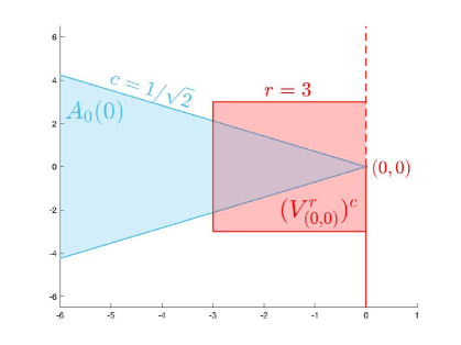
   (a) Integration set $A_{0}(0)$ for $c=1/\sqrt{2}$ together with the complement of $V_{(0,0)}^{r}$ for $r=3$.

   

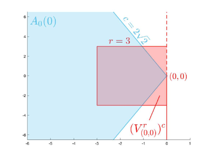
   (b) Integration set $A_{0}(0)$ for $c=2\sqrt{2}$ together with the complement of $V_{(0,0)}^{r}$ for $r=3$.

   

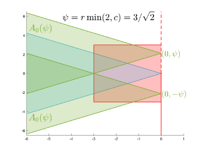
   (c) Integration set $A_{0}(0)$ together with $A_{0}(\psi)$ and $A_{0}(-\psi)$ for $\psi=r\min(2,c)$.

   

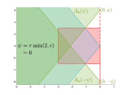
   (d) Integration set $A_{0}(0)$ together with $A_{0}(\psi)$ and $A_{0}(-\psi)$ for $\psi=r\min(2,c)$.

   

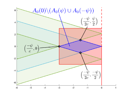
   (e) Integration set of $\boldsymbol{Z}_{0}^{(\psi)}(0)$ together with the complement of $V_{(0,0)}^{r}$.

   

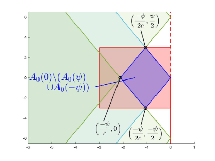
   (f) Integration set of $\boldsymbol{Z}_{0}^{(\psi)}(0)$ together with the complement of $V_{(0,0)}^{r}$.

   Figure 8: Integration set and truncated integration set of an MMAF $\boldsymbol{Z}_{t}(x)$, exemplary for $(t,x)=(0,0)$.

2. In this proof, we indicate the spatial components and write $x_{i_{a}}=(y_{i_{a}},z_{i_{a}})\in\mathbb{R}\times\mathbb{R}$ and $x_{j_{b}}=(y_{j_{b}},z_{j_{b}})\in\mathbb{R}\times\mathbb{R}$ for $a\in\{1,\ldots,u\}$ and $b\in\{1,\ldots,v\}$. Without loss of generality, let us then determine the truncated set when $(t_{j_{b}},y_{j_{b}},z_{j_{b}})=(0,0,0)$. To this end, we use four additional ambit sets that are translated by a value $\psi>0$ along both spatial axis, namely, the cones $A_{0}(\psi,\psi)$, $A_{0}(\psi,-\psi)$, $A_{0}(-\psi,\psi)$ and $A_{0}(-\psi,-\psi)$, as illustrated in Figure 10-(c) for $c\leq 1$ and in Figure 10-(d) for $c>1$). Then, we set the truncated integration set to $B_{0}^{\psi}(0)=A_{0}(0,0)\backslash(A_{0}(\psi,\psi)\cup A_{0}(\psi,-\psi)\cup A_{0}(-\psi,\psi)\cup A_{0}(-\psi,-\psi))$. Since $(t_{i_{a}},y_{i_{a}},z_{i_{a}})\in V_{(0,0,0)}^{r}$, it is sufficient to choose $\psi$ such that the integration set of $\boldsymbol{Z}_{0}^{(\psi)}(0,0)$ is a subset of $(V_{(0,0,0)}^{r})^{c}$, i.e.

   $$\sup_{b\in B_{0}^{\psi}(0)}\lVert b\rVert_{\infty}\leq r.$$ (69)

   In the following we prove that the choice $\psi=r\min(1,c/\sqrt{2})$ is sufficient for (69) to hold. We investigate cross sections of the truncated integration set $B_{0}^{\psi}(0)$ along the time axis. For a fixed time point $t$, we call this cross-section $B^{t}$ and, similarly, we denote the cross-section of an ambit set by $A^{t}$. Note that the cross sections of our ambit sets along the time axis are circles with radius $|ct|$ (see also Figure 9).

   1. As the distance between the center of the circle $A_{0}^{t}(0,0)$ and the centers of the circles $A_{0}^{t}(\psi,\psi)$, $A_{0}^{t}(-\psi,\psi)$, $A_{0}^{t}(\psi,-\psi)$, $A_{0}^{t}(-\psi,-\psi)$ is $\sqrt{2}\psi$, respectively, the set $A_{0}^{t}(0,0)$ (which is a circle with radius $|ct|$) is disjoint from every of the additional ambit sets’ cross-sections at $t$ and hence $B^{t}=A^{t}_{0}(0,0)$ (see Figure 9-(a)). Clearly, we obtain

      $$\sup_{t\in\big{(}-\psi/(\sqrt{2}c),0\big{]}}\sup_{b\in B^{t}}\lVert b\rVert=\sup_{t\in\big{(}-\psi/(\sqrt{2}c),0\big{]}}\max(c|t|,|t|)=\max\left(\frac{\psi}{\sqrt{2}},\frac{\psi}{\sqrt{2}c}\right).$$ (70)

   2. For such $t$ the set $A_{0}^{t}(0,0)$ intersects with every additional ambit sets’ cross-section (see Figure 9-(b)). However, as the additional ambit sets’ cross-sections do not intersect with each other, the point $p_{1}(t)=(t,c|t|,0)\in B^{t}$ on the boundary of $A_{0}^{t}(0,0)$ (see the red point in Figure 9-(b)) is not excluded from $B^{t}$ by any additional ambit set. Note that symmetry makes it sufficient to look at $p_{1}(t)$. Hence, we obtain

      $$\sup_{t\in\big{(}-\psi/c,-\psi/(\sqrt{2}c)\big{]}}\sup_{b\in B^{t}}\lVert b\rVert=\sup_{t\in\big{(}-\psi/c,-\psi/(\sqrt{2}c)\big{]}}\lVert p_{1}(t)\rVert=\max\left(\psi,\frac{\psi}{c}\right).$$ (71)

   3. For such $t$ the set $A_{0}^{t}(0,0)$ intersects with every additional ambit sets’ cross-section. Such intersection additionally restrict $A_{0}^{t}(0,0)$ (see Figure 9-(c)). Straightforward calculations show that the point where the boundaries of $A_{0}^{t}(-\psi,\psi)$ and $A_{0}^{t}(-\psi,\psi)$ as well as the set $A_{0}^{t}(0,0)$ intersect, say $p_{2}(t)$, is given by $(t,0,\psi-\sqrt{(ct)^{2}-\psi^{2}})$ (see red point in Figure 9-(c)). Note that symmetry makes it sufficient to look at $p_{2}(t)$. We obtain

      $$\sup_{t\in\big{(}-\sqrt{2}\psi/c,-\psi/c\big{]}}\sup_{b\in B^{t}}\lVert b\rVert=\sup_{t\in\big{(}-\sqrt{2}\psi/c,-\psi/c\big{]}}\lVert p_{2}(t)\rVert=\max\left(\psi,\frac{\sqrt{2}\psi}{c}\right).$$ (72)

   4. In the following, we show that for such $t$, the set $A^{t}(0,0)$ is entirely included in the union of the additional ambit sets’ cross sections. Clearly, this is true if the upper point where the boundaries of $A_{0}^{t}(-\psi,\psi)$ and $A_{0}^{t}(-\psi,\psi)$ intersect, say $p_{3}(t)$, is outside of $A_{0}^{t}(0,0)$ (see the red point in Figure 9-(d)). Note that symmetry makes it sufficient to look at $p_{3}(t)$. As straightforward calculations show that $p_{3}(t)=(t,0,\psi+\sqrt{(ct)^{2}-\psi^{2}})$, this is true if $\psi+\sqrt{(ct)^{2}-\psi^{2}}\geq c|t|$, or equivalently $(\psi+\sqrt{(ct)^{2}-\psi^{2}})^{2}\geq(ct)^{2}$. Moreover, we have

      $$\psi^{2}+2\psi\sqrt{(ct)^{2}-\psi^{2}}+(ct)^{2}-\psi^{2}\geq(ct)^{2}\iff\psi\geq 0.$$ (73)

   In view of condition (69) we combine (70), (71) and (72) and set $\psi=r\min(1,c/\sqrt{2})$, which also satisfies (73).

   In addition to the cross sectional views from Figure 9, we give a full three-dimensional view of the set $B_{0}^{\psi}(0)$ for $c\leq 1$ in Figure 10-(e) and for $c>1$ in Figure 10-(f) that highlight the points on the boundary of $B_{0}^{\psi}(0)$ with maximal $\infty$-norm for $\psi=r\min(1,c/\sqrt{2})$.
   

   Therefore, because of Proposition A.6-(ii), we can conclude that

   $$\theta_{lex}(r)\leq 2Var(\Lambda^{\prime})^{1/2}\left(\int_{0}^{\infty}\int_{A_{0}(0,0)\cap(A_{0}(\psi,\psi)\cup A_{0}(-\psi,\psi)\cup A_{0}(\psi,-\psi)\cup A_{0}(-\psi,-\psi))}f(A,-s)^{2}dsd\xi\pi(d\lambda)\right)^{1/2}$$

   $$=2Var(\Lambda^{\prime})^{1/2}\Bigg{(}\int_{0}^{\infty}\int_{A_{0}(0,0)\cap A_{0}(\psi,\psi)}f(A,-s)^{2}dsd\xi\pi(d\lambda)$$

   $$\qquad\qquad\qquad+\int_{0}^{\infty}\int_{A_{0}(0,0)\cap A_{0}(-\psi,\psi)}f(A,-s)^{2}dsd\xi\pi(d\lambda)$$

   $$\qquad\qquad\qquad+\int_{0}^{\infty}\int_{A_{0}(0,0)\cap A_{0}(\psi,-\psi)}f(A,-s)^{2}dsd\xi\pi(d\lambda)$$

   $$\qquad\qquad\qquad+\int_{0}^{\infty}\int_{A_{0}(0,0)\cap A_{0}(-\psi,-\psi)}f(A,-s)^{2}dsd\xi\pi(d\lambda)$$

   $$\qquad\qquad\qquad-\int_{0}^{\infty}\int_{A_{0}(0)\cap A_{0}(\psi,-\psi)\cap A_{0}(-\psi,-\psi)}f(A,-s)^{2}dsd\xi\pi(d\lambda)$$

   $$\qquad\qquad\qquad-\int_{0}^{\infty}\int_{A_{0}(0)\cap A_{0}(-\psi,\psi)\cap(A_{0}(\psi,-\psi)\cup A_{0}(-\psi,-\psi))}f(A,-s)^{2}dsd\xi\pi(d\lambda)$$

   $$\qquad\qquad\qquad-\int_{0}^{\infty}\int_{A_{0}(0)\cap A_{0}(\psi,\psi)\cap(A_{0}(-\psi,\psi)\cup A_{0}(\psi,-\psi)\cup A_{0}(-\psi,-\psi))}f(A,-s)^{2}dsd\xi\pi(d\lambda)\Bigg{)}^{1/2}$$

   $$\leq 2\sqrt{2Cov(\boldsymbol{Z}_{0}(0,0),\boldsymbol{Z}_{0}(\psi,\psi))+2Cov(\boldsymbol{Z}_{0}(0,0),\boldsymbol{Z}_{0}(\psi,-\psi))}.$$

which converges to zero as $r\to\infty$ for the dominated convergence theorem.    

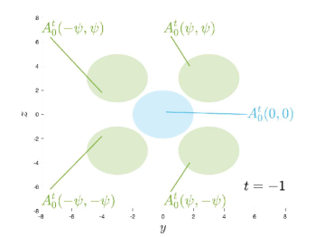
(a) Cross sections of the auxiliary ambit sets and $A_{0}^{t}(0,0)$ for $t=-1$ and $c=2$.

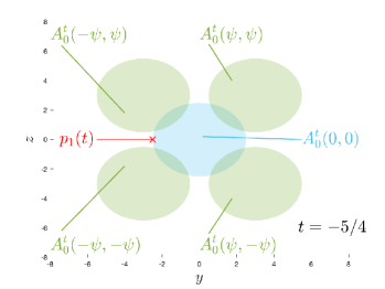
(b) Cross sections of the auxiliary ambit sets and $A_{0}^{t}(0,0)$ for $t=-5/4$ and $c=2$.

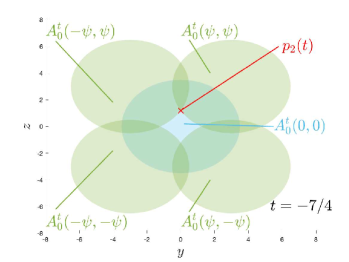
(c) Cross sections of the auxiliary ambit sets and $A_{0}^{t}(0,0)$ for $t=-7/4$ and $c=2$.

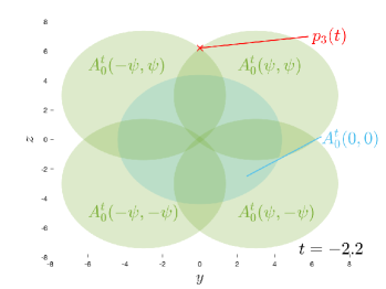
(d) Cross sections of the auxiliary ambit sets and $A_{0}^{t}(0,0)$ for $t=-2.2$ and $c=2$.

Figure 9: Cross sections of the auxiliary ambit sets and $A_{0}^{t}(0,0)$ at different time points for $\psi=3$.

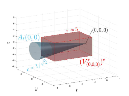
(a) Integration set $A_{0}(0,0)$ for $c=1/\sqrt{2}$ together with the complement of $V_{(0,0,0)}^{r}$ for $r=3$.

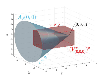
(b) Integration set $A_{0}(0,0)$ for $c=2$ together with the complement of $V_{(0,0,0)}^{r}$ for $r=3$.

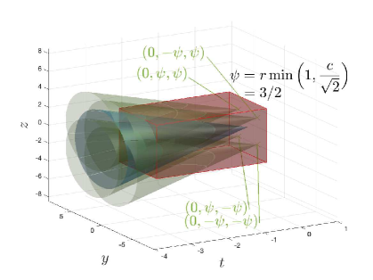
(c) Integration set $A_{0}(0,0)$ together with $A_{0}(\psi,\psi)$, $A_{0}(-\psi,\psi)$, $A_{0}(\psi,-\psi)$ and $A_{0}(-\psi,-\psi)$ for $\psi=r\min(1,c/\sqrt{2})$.

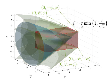
(d) Integration set $A_{0}(0,0)$ together with $A_{0}(\psi,\psi)$, $A_{0}(-\psi,\psi)$, $A_{0}(\psi,-\psi)$ and $A_{0}(-\psi,-\psi)$ for $\psi=r\min(1,c/\sqrt{2})$.

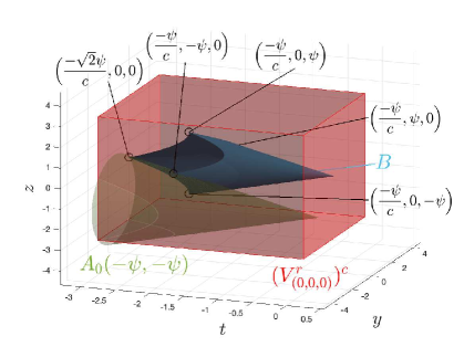
(e) $B$ is the integration set of $\boldsymbol{Z}_{0}^{(\psi)}(0,0)$. In addition, we illustrate $A_{0}(-\psi,-\psi)$ for $c=1/\sqrt{2}$ together with the complement of $V_{(0,0,0)}^{r}$ for $r=3$.

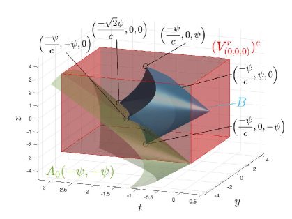
(f) $B$ is the integration set of $\boldsymbol{Z}_{0}^{(\psi)}(0,0)$. In addition, we illustrate $A_{0}(-\psi,-\psi)$ for $c=2$ together with the complement of $V_{(0,0,0)}^{r}$ for $r=3$.

Figure 10: Integration set and truncated integration set of an MMAF $\boldsymbol{Z}_{t}(y,z)$ for $d=2$.

B.2 Proofs of Section 3

Proof of Proposition 3.2.

We drop the bold notations indicating random fields and stochastic processes in the following. Let $h\in\mathcal{H}$, we call $L_{i}=L(h(X_{i}),Y_{i})$ for $i\in\mathbb{Z}$, $Z_{t}^{(M)}(x):=Z_{t}(x)\vee(-M)\wedge M$ for $M>1$, and $L^{(M)}=(L(h(X_{i}^{(M)}),Y_{i}^{(M)}))_{i\in\mathbb{Z}}$ where

$$X_{i}^{(M)}=L^{-(M)}_{p}(t_{0}+ia,x^{*}),\,\,\,\,\textrm{and}\,\,\,\,\,Y_{i}^{(M)}=Z_{t_{0}+ia}^{(M)}(x^{*}),\,\,\,\textrm{for $i\in\mathbb{Z}$},$$

and

$$L^{-(M)}_{p}(t,x^{*})=\{Z_{s}^{(M)}(\xi):(s,\xi)\in\mathbb{Z}\times\mathbb{L},\,\,\|x^{*}-\xi\|\leq c\,(t-s)\,\,\textrm{and}\,\,t-s\leq p\}.$$

for $t=t_{0}+ia$ with $i\in\mathbb{Z}$. For $u\in\mathbb{N}$, $i_{1}\leq i_{2}\leq\ldots\leq i_{u}\leq i_{u}+k=j$ with $k\in\mathbb{N}$, let us consider the marginal of the field

$$\Big{(}(X_{i_{1}},Y_{i_{1}}),\ldots,(X_{i_{u}},Y_{i_{u}}),(X_{j},Y_{j})\Big{)},$$ (74)

and let us define

$$\Gamma=\{\textrm{$(t_{i},x_{i})\in\mathbb{Z}^{1+d}$: $Z_{t_{i}}(x_{i})\in L_{p}^{-}(t_{0}+{i_{s}}a,x^{*})$ or $(t_{i},x_{i})=(t_{0}+{i_{s}}a,x^{*})$ for $s=1,\ldots,u$}\},$$

and

$$\Gamma^{\prime}=\{\textrm{$(t_{i},x_{i})\in\mathbb{Z}^{1+d}$: $Z_{t_{i}}(x_{i})\in L_{p}^{-}(t_{0}+{j}a,x^{*})$ or $(t_{i},x_{i})=(t_{0}+{j}a,x^{*})$}\}.$$

Then $r=dist(\Gamma,\Gamma^{\prime})$. In particular $\Gamma\subset V_{\Gamma^{\prime}}^{r}$, and $r=(j-i_{u})a-p$. For $F\in\mathcal{G}^{*}_{u}$ and $G\in\mathcal{G}_{1}$, then

$$|Cov(F(L_{i_{1}},\ldots,L_{i_{u}}),G(L_{j}))|$$ (75)

$$\leq |Cov(F(L_{i_{1}},\ldots,L_{i_{u}}),G(L_{j})-G(L_{j}^{(M)}))|$$ (76)

$$+|Cov(F(L_{i_{1}},\ldots,L_{i_{u}}),G(L_{j}^{(M)}))|.$$ (77)

The summand (76) is less than or equal to

$$2\|F\|_{\infty}Lip(G)\mathbb{E}[|L_{j}-L_{j}^{(M)}|] \leq 2\|F\|_{\infty}Lip(G)(\mathbb{E}[|Y_{j}-Y_{j}^{(M)}|]+\mathbb{E}[|h(X_{j})-h(X_{j}^{(M)})|])$$

$$\leq 2\|F\|_{\infty}Lip(G)(Lip(h)a(p,c)+1)\mathbb{E}[|Z_{t_{1}}(x_{1})-Z_{t_{1}}^{(M)}(x_{1})|]$$

by stationarity of the field Z, and because $L$ and $h$ are Lipschitz functions. Moreover, the function $G(L_{j}^{(M)})$ belongs to $\mathcal{G}_{a(p,c)+1}$. Let $(X,Y),(X^{\prime},Y^{\prime})\in\mathbb{R}^{a(p,c)+1}$, then

$$|G(L(h(X^{(M)}),Y^{(M)}))-G(L(h(X^{\prime(M)}),Y^{\prime(M)}))| \leq Lip(G)|L(h(X^{(M)}),Y^{(M)})-L(h(X^{\prime(M)}),Y^{\prime(M)})|$$

$$\leq Lip(G)(|h(X^{(M)}))-h(X^{\prime(M)})|+|Y^{(M)}-Y^{\prime(M)}|$$

$$\leq Lip(G)(Lip(h)+1)(\|X-X^{\prime}\|_{1}+|Y-Y^{\prime}|),$$

and $Lip(G(L_{j}^{(M)}))\leq Lip(G)(Lip(h)+1)$.

Because $Z$ is a $\theta$-lex weakly dependent random field, (77) is less than or equal to

$$\tilde{d}\|F\|_{\infty}Lip(G)(Lip(h)+1)\theta_{lex}(r).$$

We choose now $M=r$ and obtain that (75) is less than or equal than

$$\|F\|_{\infty}Lip(G)\tilde{d}(Lip(h)a(p,c)+1)\Big{(}\frac{2}{\tilde{d}}\mathbb{E}[|Z_{t_{1}}(x_{1})-Z_{t_{1}}^{(r)}(x_{1})|]+\theta_{lex}(r)\Big{)}.$$

The quantity above converges to zero as $r\to\infty$. Therefore, $(L_{i})_{i\in\mathbb{Z}}$ is a $\theta$-weakly dependent process.    

Remark B.3.

Note that when working with a general $\theta$-weakly dependent random field, as for example in Proposition 3.2, we do not employ the truncated random field defined in (66). This happens because a $\theta$-lex weakly dependent field is not generally defined as an integral driven by a Lévy basis on an ambit set. The field (66) can just be employed in the MMAF framework. In a more general framework, without further information on the structure of the field, we can just employ the truncated random field $\boldsymbol{Z}_{t}^{(M)}(x):=\boldsymbol{Z}_{t}(x)\vee(-M)\wedge M$.

Proof of Proposition 3.6.

We drop the bold notations indicating random fields and stochastic processes in the following. We call $L_{i}=L(h(X_{i}),Y_{i})$ for $i\in\mathbb{Z}$, as defined in Proposition B.1. Moreover we employ the truncated field $Z_{t}^{(\psi)}(x)$ and define $L^{(\psi)}=(L(h_{\beta}(X_{i}^{(\psi)}),Y_{i}^{(\psi)}))_{i\in\mathbb{Z}}$ where

$$X_{i}^{(\psi)}=L^{-(\psi)}_{p}(t_{0}+ia,x^{*}),\,\,\,\,\textrm{and}\,\,\,\,\,Y_{i}^{(\psi)}=Z_{t_{0}+ia}^{(\psi)}(x^{*}),\,\,\,\textrm{for $i\in\mathbb{Z}$},$$

and

$$L^{-(\psi)}_{p}(t,x^{*})=\{Z_{s}^{(\psi)}(\xi):(s,\xi)\in\mathbb{Z}\times\mathbb{L},\,\,\|x^{*}-\xi\|\leq c\,(t-s)\,\,\textrm{and}\,\,t-s\leq p\}.$$

for $t=t_{0}+ia$ with $i\in\mathbb{Z}$. For $u\in\mathbb{N}$, $i_{1}\leq i_{2}\leq\ldots\leq i_{u}\leq i_{u}+k=j$ with $k\in\mathbb{N}$, let us consider the marginal of the field

$$\Big{(}(X_{i_{1}},Y_{i_{1}}),\ldots,(X_{i_{u}},Y_{i_{u}}),(X_{j},Y_{j})\Big{)},$$ (78)

and let us define

$$\Gamma=\{\textrm{$(t_{i},x_{i})\in\mathbb{Z}^{1+d}$: $Z_{t_{i}}(x_{i})\in L_{p}^{-}(t_{0}+{i_{s}}a,x^{*})$ or $(t_{i},x_{i})=(t_{0}+{i_{s}}a,x^{*})$ for $s=1,\ldots,u$}\},$$

and

$$\Gamma^{\prime}=\{\textrm{$(t_{i},x_{i})\in\mathbb{Z}^{1+d}$: $Z_{t_{i}}(x_{i})\in L_{p}^{-}(t_{0}+{j}a,x^{*})$ or $(t_{i},x_{i})=(t_{0}+{j}a,x^{*})$}\}.$$

Then $r=dist(\Gamma,\Gamma^{\prime})$. In particular $\Gamma\subset V_{\Gamma^{\prime}}^{r}$, and $r=(j-i_{u})a-p$. For $F\in\mathcal{G}^{*}_{u}$ and $G\in\mathcal{G}_{1}$, then

$$|Cov(F(L_{i_{1}},\ldots,L_{i_{u}}),G(L_{j}))|$$

$$\leq |Cov(F(L_{i_{1}},\ldots,L_{i_{u}}),G(L_{j})-G(L_{j}^{(\psi)}))|$$ (79)

$$+|Cov(F(L_{i_{1}},\ldots,L_{i_{u}}),G(L_{j}^{(\psi)}))|.$$ (80)

The summand (80) is equal to zero because $\Gamma\subset V_{\Gamma^{\prime}}^{r}$, see proof of Proposition 2.16 for more details about this part of the proof. We can then bound (79) from above by

$$2\|F\|_{\infty}Lip(G)\mathbb{E}[|L_{j}-L_{j}^{(\psi)}|] \leq 2\|F\|_{\infty}Lip(G)(\mathbb{E}[|Y_{j}-Y_{j}^{(\psi)}|]+\mathbb{E}[|h(X_{j})-h(X_{j}^{(\psi)})|])$$ (81)

$$\leq 2\|F\|_{\infty}Lip(G)(Lip(h)a(p,c)+1)\mathbb{E}[|Z_{t_{1}}(x_{1})-Z_{t_{1}}^{(\psi)}(x_{1})|]$$ (82)

where (81) holds because $L$ is a function with Lipschitz constant equal to one, and (82) holds given that $h$ is Lipschitz.

When we work with linear functions, we consider $h$ parameterized with respect to the set $B\in\mathbb{R}^{a(p,c)}$

$$\mathbb{E}[|h_{\beta}(X_{j})-h_{\beta}(X_{j}^{(\psi)})\|]=\mathbb{E}\Big{[}\Big{|}\sum_{l=1}^{a(p,c)}\beta_{1,l}(Z_{t_{l}}(x_{l})-Z_{t_{l}}^{(\psi)}(x_{l}))\Big{|}\Big{]}.$$ (83)

By stationarity of the field $Z$, we have that (83) is smaller or equal than $\|\beta_{1}\|_{1}\mathbb{E}[|Z_{t_{1}}(x_{1})-Z_{t_{1}}^{(\psi)}(x_{1})|]$. Overall, we have that (79) is smaller or equal than

$$2\|F\|_{\infty}Lip(G)(Lip(h)a(p,c)+1)\mathbb{E}[|Z_{t_{1}}(x_{1})-Z_{t_{1}}^{(\psi)}(x_{1})|]\,\,\,\textrm{for $h$ a Lipschitz function,}$$

or it is smaller or equal than

$$2\|F\|_{\infty}Lip(G)(\|\beta_{1}\|_{1}+1)\mathbb{E}[|Z_{t_{1}}(x_{1})-Z_{t_{1}}^{(\psi)}(x_{1})|]\,\,\,\textrm{for $h_{\beta}$ a linear function}.$$

Because of the properties of the truncated field $Z_{t_{1}}^{(\psi)}(x_{1})$, we have that the above bounds converge to zero as $r\to\infty$. Therefore, $L$ is a $\theta$-weakly dependent process.    

The proof of Theorem 3.7 uses a blocks technique introduced in the papers [40] and [51]. Such results are based on the use of several lemmas. To ease the complete understanding of the proof of Theorem 3.7, we prove these Lemmas below, given that they undergo several modifications in our framework. Let us start by partitioning a set $\{1,2,\ldots,m\}$ into $k$ blocks. Each block will contain $l=\lfloor\frac{m}{k}\rfloor$ terms. Let $h=m-k\,l<k$ denote the remainder when we divide $m$ by $k$. We now construct $k$ blocks such that the number of elements in the $j$th-block is defined by

$$\bar{l}_{j}=\left\{\begin{array}[]{ll}l+1&\textrm{if}\,\,\,j=1,2,\ldots,h\\ l&\textrm{if}\,\,\,j=h+1,\ldots,k\end{array}\right..$$

Let $(\boldsymbol{U}_{i})_{i\in\mathbb{Z}}$ a stationary process, and $\boldsymbol{V}_{m}=\sum_{i=1}^{m}\boldsymbol{U}_{i}$, for $j=1,\ldots,k$ we define the $j$-th block as

$$\boldsymbol{V}_{j,m}=\boldsymbol{U}_{j}+\boldsymbol{U}_{j+k}+\ldots\boldsymbol{U}_{j+(\bar{l}_{j}-1)\,k}=\sum_{i=1}^{\bar{l}_{j}}\boldsymbol{U}_{j+(i-1)\,k}$$

such that

$$\boldsymbol{V}_{m}=\sum_{j=1}^{k}\boldsymbol{V}_{j,m}=\sum_{j=1}^{k}\sum_{i=1}^{\bar{l}_{j}}\boldsymbol{U}_{j+(i-1)\,k}.$$

For $j=1,2,\ldots,k$, let us define $p_{j}=\frac{\bar{l}_{j}}{m}$. It follows that $\sum_{j=1}^{k}p_{j}=\frac{1}{m}\sum_{j=1}^{k}\bar{l}_{j}=1$.

Lemma B.4.

For all $s\in\mathbb{R}$

$$\mathbb{E}\Big{[}\exp\Big{(}s\frac{\boldsymbol{V}_{m}}{m}\Big{)}\Big{]}\leq\sum_{j=1}^{k}p_{j}\mathbb{E}\Big{[}\exp\Big{(}s\frac{\boldsymbol{V}_{j,m}}{\bar{l}_{j}}\Big{)}\Big{]}$$

The proof of the result above is due to Hoeffding [42].

Lemma B.5.

Let the assumptions of Theorem 3.7 hold and define the process $(\boldsymbol{U}_{i})_{i\in\mathbb{Z}}$ such that $\boldsymbol{U}_{i}:=f(\boldsymbol{Z}_{i})-\mathbb{E}[f(\boldsymbol{Z}_{i})]$. For all $j=1,2,\ldots,k$, $l\geq 2$ and $0<s<\frac{3l}{|b-a|}$

$$M_{\bar{l}_{j}}(s)=\Big{|}\mathbb{E}\Big{[}\prod_{i=1}^{\bar{l}_{j}}\exp\Big{(}\frac{s\,\boldsymbol{U}_{j+(i-1)\,k}}{\bar{l}_{j}}\Big{)}\Big{]}-\prod_{i=1}^{\bar{l}_{j}}\mathbb{E}\Big{[}\exp\Big{(}\frac{s\,\boldsymbol{U}_{j+(i-1)\,k}}{\bar{l}_{j}}\Big{)}\Big{]}\Big{|}\leq\exp(s\,|b-a|)\theta(k)s$$ (84)

The same result holds when defining the process $(\boldsymbol{U}_{i})_{i\in\mathbb{Z}}$ for $\boldsymbol{U}_{i}=\mathbb{E}[f(\boldsymbol{X}_{i})]-f(\boldsymbol{X}_{i})$.

Proof.

Let us first discuss the case when $\boldsymbol{U}_{i}=f(\boldsymbol{X}_{i})-\mathbb{E}[f(\boldsymbol{X}_{i})]$, we have that the process $\boldsymbol{U}$ has mean zero and $|\boldsymbol{U}_{i}|\leq|b-a|$. Let us define $\mathcal{F}_{j}=\sigma(\boldsymbol{U}_{i},i\leq j)$.

$$M_{\bar{l}_{j}} :=\Bigg{|}\mathbb{E}\Big{[}\prod_{i=1}^{\bar{l}_{j}}\exp\Big{(}\frac{s\boldsymbol{U}_{j+(i-1)k}}{\bar{l}_{j}}\Big{)}\Big{]}-\prod_{i=1}^{\bar{l}_{j}}\mathbb{E}\Big{[}\exp\Big{(}\frac{s\boldsymbol{U}_{j+(i-1)k}}{\bar{l}_{j}}\Big{)}\Big{]}\Bigg{|}$$

$$=\Bigg{|}\mathbb{E}\Big{[}\prod_{i=1}^{\bar{l}_{j}-1}\exp\Big{(}\frac{s\boldsymbol{U}_{j+(i-1)k}}{\bar{l}_{j}}\Big{)}\mathbb{E}\Big{[}\exp\Big{(}\frac{s\boldsymbol{U}_{j+(\bar{l}_{j}-1)k}}{\bar{l}_{j}}\Big{)}\Big{|}\mathcal{F}_{j+(\bar{l}_{j}-2)k}\Big{]}\Big{]}-\prod_{i=1}^{\bar{l}_{j}}\mathbb{E}\Big{[}\exp\Big{(}\frac{s\boldsymbol{U}_{j+(i-1)k}}{\bar{l}_{j}}\Big{)}\Big{]}\Bigg{|}$$

$$\leq\Bigg{|}\mathbb{E}\Big{[}\prod_{i=1}^{\bar{l}_{j}-1}\exp\Big{(}\frac{s\boldsymbol{U}_{j+(i-1)k}}{\bar{l}_{j}}\Big{)}\Big{(}\mathbb{E}\Big{[}\exp\Big{(}\frac{s\boldsymbol{U}_{j+(\bar{l}_{j}-1)k}}{\bar{l}_{j}}\Big{)}\Big{|}\mathcal{F}_{j+(\bar{l}_{j}-2)k}\Big{]}-\mathbb{E}\Big{[}\exp\Big{(}\frac{s\boldsymbol{U}_{j+(\bar{l}_{j}-1)k}}{\bar{l}_{j}}\Big{)}\Big{]}\Big{)}\Big{]}\Bigg{|}$$

$$+\Bigg{|}\mathbb{E}\Big{[}\exp\Big{(}\frac{s\boldsymbol{U}_{j+(\bar{l}_{j}-1)k}}{\bar{l}_{j}}\Big{)}\Big{]}\Bigg{|}\,\,\Bigg{|}\mathbb{E}\Big{[}\prod_{i=1}^{\bar{l}_{j}-1}\exp\Big{(}\frac{s\boldsymbol{U}_{j+(i-1)k}}{\bar{l}_{j}}\Big{)}\Big{]}-\prod_{i=1}^{\bar{l}_{j}-1}\mathbb{E}\Big{[}\exp\Big{(}\frac{s\boldsymbol{U}_{j+(i-1)k}}{\bar{l}_{j}}\Big{)}\Big{]}\Bigg{|}$$

$$\leq\Bigg{\|}\prod_{i=1}^{\bar{l}_{j}-1}\exp\Big{(}\frac{s\boldsymbol{U}_{j+(i-1)k}}{\bar{l}_{j}}\Big{)}\Bigg{\|}_{\infty}\mathbb{E}\Big{[}\Big{|}\mathbb{E}\Big{[}\exp\Big{(}\frac{s\boldsymbol{U}_{j+(\bar{l}_{j}-1)k}}{\bar{l}_{j}}\Big{)}\Big{|}\mathcal{F}_{j+(\bar{l}_{j}-2)k}\Big{]}-\mathbb{E}\Big{[}\exp\Big{(}\frac{s\boldsymbol{U}_{j+(\bar{l}_{j}-1)k}}{\bar{l}_{j}}\Big{)}\Big{]}\Big{|}\Big{]}$$

$$+\Bigg{\|}\exp\Big{(}\frac{s\boldsymbol{U}_{j+(\bar{l}_{j}-1)k}}{\bar{l}_{j}}\Big{)}\Bigg{\|}_{\infty}M_{\bar{l}_{j}-1}$$

The above is then less than or equal to

$$\exp\Big{(}\frac{s(\bar{l}_{j}-1)|b-a|}{\bar{l}_{j}}\Big{)}\exp\Big{(}\frac{-s|a|}{\bar{l}_{j}}\Big{)}\mathbb{E}\Bigg{[}\Bigg{|}\mathbb{E}\Bigg{[}\exp\Bigg{(}\frac{sf(\boldsymbol{Z}_{j+(\bar{l}_{j}-1)k})}{\bar{l}_{j}}\Bigg{)}\Bigg{|}\mathcal{F}_{j+(\bar{l}_{j}-2)k}\Bigg{]}$$ (85)

$$-\mathbb{E}\Bigg{[}\exp\Bigg{(}\frac{sf(\boldsymbol{Z}_{j+(\bar{l}_{j}-1)k})}{\bar{l}_{j}}\Bigg{)}\Bigg{]}\Bigg{|}\Bigg{]}+\exp\Big{(}\frac{s|b-a|}{\bar{l}_{j}}\Big{)}M_{\bar{l}_{j}-1}.$$

Note that the function $g(x)=\frac{\exp\Big{(}\frac{sx}{\bar{l}_{j}}\Big{)}}{\exp\Big{(}\frac{s|b|}{\bar{l}_{j}}\Big{)}\frac{s}{\bar{l}_{j}}}1_{\mathcal{A}}(x)$ is in $\mathcal{L}_{1}$ for each $s$, where $\mathcal{A}=\{x:|x|\leq|b-a|\}$. We then use the mixingales-type representation of the $\theta$-coefficients of $f(\boldsymbol{Z})$, and obtain that

$$M_{\bar{l}_{j}}\leq\exp\Big{(}\frac{s\bar{l}_{j}|b-a|}{\bar{l}_{j}}\Big{)}\theta(k)\frac{s}{\bar{l}_{j}}+\exp\Big{(}\frac{s|b-a|}{\bar{l}_{j}}\Big{)}M_{\bar{l}_{j}-1}.$$

Let now, $u=\exp\Big{(}\frac{s|b-a|}{\bar{l}_{j}}\Big{)}$, we have that

$$M_{\bar{l}_{j}} \leq\theta(k)u^{\bar{l}_{j}}\frac{s}{\bar{l}_{j}}+uM_{\bar{l}_{j}-1}$$

$$\leq(\bar{l}_{j}-2)\theta(k)u^{\bar{l}_{j}}\frac{s}{\bar{l}_{j}}+u^{\bar{l}_{j}-2}\Big{|}\mathbb{E}\Big{[}\exp\Big{(}\frac{s\boldsymbol{U}_{j}}{\bar{l}_{j}}\Big{)}\exp\Big{(}\frac{s\boldsymbol{U}_{j+k}}{\bar{l}_{j}}\Big{)}\Big{]}-\mathbb{E}\Big{[}\exp\Big{(}\frac{s\boldsymbol{U}_{j}}{\bar{l}_{j}}\Big{)}\Big{]}\mathbb{E}\Big{[}\exp\Big{(}\frac{s\boldsymbol{U}_{j+k}}{\bar{l}_{j}}\Big{)}\Big{]}\Big{|}$$

$$\leq(\bar{l}_{j}-2)\theta(k)u^{\bar{l}_{j}}\frac{s}{\bar{l}_{j}}+u^{\bar{l}_{j}-1}\Big{|}\mathbb{E}\Big{[}\exp\Big{(}\frac{s\boldsymbol{U}_{j+k}}{\bar{l}_{j}}\Big{)}|\mathcal{F}_{j}\Big{]}-\mathbb{E}\Big{[}\exp\Big{(}\frac{sU_{j+k}}{\bar{l}_{j}}\Big{)}\Big{]}\Big{|}$$

$$\leq(\bar{l}_{j}-1)\theta(k)u^{\bar{l}_{j}}\frac{s}{\bar{l}_{j}}=(\bar{l}_{j}-1)\exp\Big{(}s|b-a|\Big{)}\theta(k)\frac{s}{\bar{l}_{j}}.$$

In conclusion, for all $j=1,\ldots,k$ (and remembering that $\bar{l}_{j}=l$ or $\bar{l}_{j}=l+1$)

$$M_{\bar{l}_{j}}\leq\exp(s\,|b-a|)\theta(k)s.$$

Similar calculations apply when $\boldsymbol{U}_{i}=\mathbb{E}[f(\boldsymbol{Z}_{i})]-f(\boldsymbol{Z}_{i})$.    

Remark B.6.

Note that by showing Lemma B.5 for $\boldsymbol{U}_{i}=\mathbb{E}[f(\boldsymbol{Z}_{i})]-f(\boldsymbol{Z}_{i})$ there is a slight change in the proof at point (85). However, in the end, the result (84) equally holds.

Lemma B.7.

Let the Assumptions of Theorem 3.7 hold and define the process $(\boldsymbol{U}_{i})_{i\in\mathbb{Z}}$ such that $\boldsymbol{U}_{i}=f(\boldsymbol{Z}_{i})-\mathbb{E}[f(\boldsymbol{Z}_{i})]$. For all $j=1,2,\ldots,k$, $l\geq 2$ and $0<s<\frac{3l}{|b-a|}$

$$\mathbb{E}\Big{[}\exp\Big{(}\frac{s\boldsymbol{V}_{j,m}}{\bar{l}_{j}}\Big{)}\Big{]}\leq\exp\Bigg{(}\frac{s^{2}\mathbb{E}[\boldsymbol{U}_{1}^{2}]}{2l\Big{(}1-\frac{s|b-a|}{3l}\Big{)}}\Bigg{)}+\exp(s\,|b-a|)\theta(k)s$$

The same result holds when defining the process $(\boldsymbol{U}_{i})_{i\in\mathbb{Z}}$ for $\boldsymbol{U}_{i}=\mathbb{E}[f(\boldsymbol{Z}_{i})]-f(\boldsymbol{Z}_{i})$.

Proof.

$$\mathbb{E}\Big{[}\exp\Big{(}\frac{s\boldsymbol{V}_{j,m}}{\bar{l}_{j}}\Big{)}\Big{]} =\mathbb{E}\Big{[}\exp\Big{(}\sum_{i=1}^{\bar{l}_{j}}\frac{s\boldsymbol{U}_{j+(i-1)\,k}}{\bar{l}_{j}}\Big{)}\Big{]}\leq\prod_{i=1}^{\bar{l}_{j}}\mathbb{E}\Big{[}\exp\Big{(}\frac{s\boldsymbol{U}_{j+(i-1)\,k}}{\bar{l}_{j}}\Big{)}\Big{]}$$

$$+\Big{|}\mathbb{E}\Big{[}\prod_{i=1}^{\bar{l}_{j}}\exp\Big{(}\frac{s\boldsymbol{U}_{j+(i-1)\,k}}{\bar{l}_{j}}\Big{)}\Big{]}-\prod_{i=1}^{\bar{l}_{j}}\mathbb{E}\Big{[}\exp\Big{(}\frac{s\boldsymbol{U}_{j+(i-1)\,k}}{\bar{l}_{j}}\Big{)}\Big{]}\Big{|}$$

$$=\mathbb{E}\Big{[}\exp\Big{(}\frac{s\boldsymbol{U}_{j+(i-1)\,k}}{\bar{l}_{j}}\Big{)}\Big{]}^{\bar{l}_{j}}+M_{\bar{l}_{j}}$$ (86)

We have that $\mathbb{E}[\boldsymbol{U}_{j+(i-1)\,k}]=0$ by definition of the process $\boldsymbol{U}$, and $\frac{\boldsymbol{U}_{j+(i-1)\,k}}{\bar{l}_{j}}$ satisfies the Bernstein moment condition (Remark A1 [51]) with $K_{1}=\frac{|b-a|}{3\bar{l}_{j}}$. Hence, for $\bar{l}_{j}\geq 2$ and $0<s<\frac{3\bar{l}_{j}}{|b-a|}$

$$\mathbb{E}\Big{[}\exp\Big{(}\frac{s\boldsymbol{U}_{j+(i-1)\,k}}{\bar{l}_{j}}\Big{)}\Big{]}\leq\exp\Bigg{(}\frac{s^{2}\mathbb{E}[(\boldsymbol{U}_{j+(i-1)k}/\bar{l}_{j})^{2}]}{2\Big{(}1-\frac{s|b-a|}{3\bar{l}_{j}}\Big{)}}\Bigg{)}.$$ (87)

Because $\bar{l}_{j}\geq l$, we can conclude that the inequality above holds for $l\geq 2$. Moreover, by stationarity of the process $\boldsymbol{U}$ and since for all $j=1,2,\ldots,k$, we can bound (86) uniformly with respect to the index $j$ by using Lemma B.5, and noticing that

$$0<s<\frac{3l}{|b-a|}\leq\frac{3\bar{l}_{j}}{|b-a|},$$

and then

$$\Big{(}1-\frac{s|b-a|}{3\bar{l}_{j}}\Big{)}\geq\Big{(}1-\frac{s|b-a|}{3l}\Big{)}.$$

The same proof applies when defining $\boldsymbol{U}_{i}=\mathbb{E}[f(\boldsymbol{Z}_{i})]-f(\boldsymbol{Z}_{i})$.

   

Proof of Theorem 3.7.

By combining Lemmas B.4, B.5, B.7, we can bound the process $\boldsymbol{U}:=f(\boldsymbol{Z})-\mathbb{E}[f(\boldsymbol{Z})]$ for $0<s<\frac{3l}{|b-a|}$ as follows:

$$\mathbb{E}\Big{[}\exp\Big{(}s\frac{1}{m}\sum_{i=1}^{m}f(\boldsymbol{Z}_{i})-\mathbb{E}[f(\boldsymbol{Z}_{i})]\Big{)}\Big{]} =\mathbb{E}\Big{[}\exp\Big{(}s\frac{1}{m}\sum_{i=1}^{m}\boldsymbol{U}_{i}\Big{)}\Big{]}=\mathbb{E}\Big{[}\exp\Big{(}\frac{s}{m}\sum_{j=1}^{k}\boldsymbol{V}_{j,m}\Big{)}\Big{]}$$

$$=\mathbb{E}\Big{[}\exp\Big{(}\frac{s}{m}\sum_{j=1}^{k}\sum_{i=1}^{\bar{l}_{j}}\boldsymbol{U}_{j+(i-1)\,k}\Big{)}\Big{]}$$

$$\leq\sum_{j=1}^{k}p_{j}\mathbb{E}\Big{[}\exp\Big{(}\frac{s\boldsymbol{V}_{j,m}}{\bar{l}_{j}}\Big{)}\Big{]}$$ (88)

$$\leq\exp\Bigg{(}\frac{s^{2}Var(f(\boldsymbol{Z}_{1}))}{2l\Big{(}1-\frac{s|b-a|}{3l}\Big{)}}\Bigg{)}+\exp(s\,|b-a|)\theta(k)s,$$ (89)

where $\boldsymbol{V}_{j,m}=\sum_{i=1}^{\bar{l}_{j}}\boldsymbol{U}_{j+(i-1)\,k}$. The inequalities (88) and (89) hold because of Lemma B.4 and Lemma B.7, respectively. We have then proved the inequality (28). The same proof applies for showing the bound (29) by defining $\boldsymbol{U}_{i}=\mathbb{E}[f(\boldsymbol{Z}_{i})]-f(\boldsymbol{Z}_{i})$ .    

We remind the reader that the proof of Theorem 3.8 and 37 make use of the below Lemma that we recall for completeness.

Lemma B.8 (Legendre transform of the Kullback-Leibler divergence function).

For any $\pi\in\mathcal{M}^{1}_{+}(B)$, for any measurable function $h:B\to\mathbb{R}$ such that $\pi[\exp(h)]\leq\infty$, we have that

$$\pi[\exp(h)]=\exp\Big{(}\sup_{\rho\in\mathcal{M}^{1}_{+}(B)}\rho[h]-KL(\rho||\pi)\Big{)},$$

with the convention $\infty-\infty=-\infty$. Moreover, as soon as $h$ is upper bounded on the support of $\pi$, the supremum with respect to $\rho$ in the right-hand side is reached for the Gibbs distribution with Radon-Nikodym derivative w.r.t. $\pi$ equal to $\frac{\exp(h)}{\pi[\exp(h)]}$.

The proof of Lemma (B.8) has been known since the work of Kullback [49] in the case of a finite space $B$, whereas the general case has been proved by Donsker and Varadhan [31]. Given this result, we are now ready to prove our PAC Bayesian bounds.

Proof of Theorem 3.8.

Let us choose $f(s)=\frac{s}{\epsilon}$ for $0<s<\epsilon$ , which satisfies the assumptions of Theorem 3.7 and has support in $[0,1]$. Let $\Delta(\beta)=\frac{\epsilon}{m}(\sum_{i=1}^{m}\mathbb{E}[f(\boldsymbol{L}_{i}^{\epsilon})]-f(\boldsymbol{L_{i}^{\epsilon}}))$. We have in this case that $\boldsymbol{U}_{i}=\mathbb{E}[f(\boldsymbol{L_{i}})]-f(\boldsymbol{L_{i}^{\epsilon}})$ such that $\mathbb{E}[\boldsymbol{U}_{i}]=0$ and $|\boldsymbol{U}_{i}|\leq 1$. Note that the process $f(\boldsymbol{L}_{i}^{\epsilon})_{i\in\mathbb{Z}}$ has the same $\theta$-weak coefficients of the process $(\boldsymbol{L}_{i}^{\epsilon})_{i\in\mathbb{Z}}$ because $f$ is a 1-Lipschitz function. By Theorem 3.7 applied for $0<\epsilon\sqrt{l}<3\sqrt{l}$, and the bound (26),

$$\mathbb{E}\Big{[}\exp\Big{(}\sqrt{l}\,\Delta(\beta)\Big{)}\Big{]}=\mathbb{E}\Big{[}\exp\Big{(}\epsilon\sqrt{l}\frac{1}{m}\sum_{i=1}^{m}\boldsymbol{U}_{i}\Big{)}\Big{]} \leq\exp\Big{(}\frac{3\epsilon^{2}}{2(3-\epsilon)}\Big{)}$$

$$+2(Lip(h)a(p,c)+1)3\sqrt{l}\exp(3\sqrt{l})\theta(k)$$ (90)

where the last equality holds because of the particular shape of the chosen function $f$.

We follow the scheme of proof developed by [13].

$$\sqrt{l}\,\hat{\rho}[R^{\epsilon}(h)]-\hat{\rho}[r^{\epsilon}(h)]=\hat{\rho}[\sqrt{l}\,(R^{\epsilon}(h)-r^{\epsilon}(h))]\hskip 14.22636pt$$

$$\leq KL(\hat{\rho}||\pi)+\log(\pi[\exp(\sqrt{l}\,(R^{\epsilon}(h)-r^{\epsilon}(h)))])\hskip 14.22636pt\textrm{($\mathbb{P}$-almost surely by Lemma \ref{kl})}.$$ (91)

We have that $\pi[\exp(\sqrt{l}\,(R^{h}(\beta)-r^{\epsilon}(h)))]:=\boldsymbol{A_{m}}$ is a random variable on $\boldsymbol{S_{m}}$. By Markov’s inequality, for $\delta\in(0,1)$

$$\mathbb{P}\Big{(}\boldsymbol{A_{m}}\leq\frac{\mathbb{E}[\boldsymbol{A_{m}}]}{\delta}\Big{)}\geq 1-\delta.$$

This in turn implies that with probability at least $1-\delta$ over $\boldsymbol{S_{m}}$

$$\hat{\rho}[R^{\epsilon}(h)]-\hat{\rho}[r^{\epsilon}(h)] \leq\frac{KL(\hat{\rho}||\pi)+\log\frac{1}{\delta}}{\sqrt{l}}+\frac{1}{\sqrt{l}}\log\Big{(}\pi\Big{[}\mathbb{E}\Big{[}\exp\Big{(}\sqrt{l}(R^{\epsilon}(h)-r^{\epsilon}(h))\Big{)}\Big{]}\Big{]}\Big{)}$$ (92)

$$\leq\frac{KL(\hat{\rho}||\pi)+\log\frac{1}{\delta}}{\sqrt{l}}+\frac{1}{\sqrt{l}}\log\Big{(}\pi\Big{[}\exp\Big{(}\frac{3\epsilon^{2}}{2(3-\epsilon)}\Big{)}+$$

$$2(Lip(h)a(p,c)+1)3\sqrt{l}\exp(3\sqrt{l})\theta(k)\Big{]}\Big{)},$$ (93)

where (92) holds by swapping the expectation over $\boldsymbol{S}_{m}$ and over $\pi$ using Fubini’s Theorem, and (93) is obtained by using (90). Similarly, it can be proven that the bound (93) holds for $\hat{\rho}[R^{\epsilon}(h)]-\hat{\rho}[r^{\epsilon}(h)]$. We then conclude by using an union bound.    

Proof of Theorem 3.12.

First of all, we need to show that $A_{m}$ defined in (33) is a super-martingale. Let $\mathcal{F}_{m}=\sigma\{\boldsymbol{S}_{m}\}$, and $\mathbb{E}_{m}[\cdot]:=\mathbb{E}[\cdot|\mathcal{F}_{m}]$ for $m>0$. By the definition of $f_{0}$, we have that $A_{0}\leq 1$. Using Lemma 2.2 in [39], we get that

$$\mathbb{E}_{m-1}[A_{m}] =\mathbb{E}_{m-1}[\pi[\exp(f_{m}(\boldsymbol{S},h))]]=\pi[\mathbb{E}_{m-1}[\exp(f_{m}(\boldsymbol{S},h))]]$$

$$=\pi[\exp(f_{m-1}(S,h))\mathbb{E}_{m-1}[\exp(\eta(\mathbb{E}[L^{\epsilon}(h(\boldsymbol{X}_{i}),\boldsymbol{Y}_{i})]-L^{\epsilon}(h(\boldsymbol{X}_{i}),\boldsymbol{Y}_{i}))$$

$$+\eta^{2}\theta_{lex}^{Decay}(k))]\leq A_{m-1}.$$

In fact, because $\theta_{lex}^{Decay}(k)<-2\epsilon$

$$\eta(\mathbb{E}[L^{\epsilon}(h(\boldsymbol{X}_{i}),\boldsymbol{Y}_{i})]-L^{\epsilon}(h(\boldsymbol{X}_{i}),\boldsymbol{Y}_{i}))+\eta^{2}\theta_{lex}^{Decay}(k)<0\,\,\,\textit{almost surely}$$

and $\mathbb{E}_{m-1}[\exp(\eta(\mathbb{E}[L^{\epsilon}(h(\boldsymbol{X}_{i}),\boldsymbol{Y}_{i})]-L^{\epsilon}(h(\boldsymbol{X}_{i}),\boldsymbol{Y}_{i}))+\eta^{2}\theta_{lex}^{Decay}(k))]<1$. $(A_{m})_{m\in\mathbb{N}}$ is a non-negative super-martingale. We can then apply the Ville’s maximal inequality, and for $\delta\in(0,1)$ we have that

$$\mathbb{P}(A_{m}\leq\frac{1}{\delta})\geq 1-\delta.$$

By Lemma B.8 applied to $f_{m}(S,h)$, we have that

$$\hat{\rho}[f_{m}(\boldsymbol{S},h)]\leq KL(\hat{\rho}||\pi)+\log(\pi[\exp(f_{m}(\boldsymbol{S},h))]).$$

Dividing both side of the inequality by $m$, we obtain that for all $m$ with probability at least $1-\delta$

$$\hat{\rho}[R^{\epsilon}(h)]-\hat{\rho}[r^{\epsilon}(h)]\leq\frac{KL(\hat{\rho}||\pi)+\log(1/\delta)}{m\eta}-\eta\theta_{lex}^{Decay}(k)$$

The same calculations can be conducted to determine an anytime bound for the quantity $\hat{\rho}[r^{\epsilon}(h)]-\hat{\rho}[R^{\epsilon}(h)]$. By using a union bound we then conclude.    

Proof of Theorem 3.16.

Let $\frac{d\bar{\rho}}{d\pi}=\frac{exp(-\sqrt{m}r^{\epsilon}(h))}{\pi[\exp(-\sqrt{m}r^{\epsilon}(h))]}$. By Lemma B.8, we have that

$$\bar{\rho}=arg\inf_{\hat{\rho}}\Big{(}K(\hat{\rho}||\pi)-\hat{\rho}[-\sqrt{m}r^{\epsilon}(h)]\Big{)}=arg\inf_{\hat{\rho}}\Big{(}\frac{K(\hat{\rho}||\pi)}{\sqrt{m}}+\hat{\rho}[r^{\epsilon}(h)]\Big{)},$$

and by using (36), for all $\delta\in(0,1)$

$$\mathbb{P}\Big{\{}\bar{\rho}[R^{\epsilon}(h)]\leq\inf_{\hat{\rho}}\Big{(}\hat{\rho}[r^{\epsilon}(h)]+\Big{(}KL(\hat{\rho}||\pi)+\log\Big{(}\frac{1}{\delta}\Big{)}\Big{)}\frac{1}{\sqrt{m}}\Big{)}-\frac{1}{\sqrt{m}}\theta_{lex}^{Decay}(1)\Big{\}}\geq 1-\delta$$ (94)

By now substituting to $\hat{\rho}[r^{\epsilon}(\beta)]$ in (94) its bound obtained in inequality (34), we obtain that

$$\mathbb{P}\Big{\{}\bar{\rho}[R^{\epsilon}(h)]\leq\inf_{\hat{\rho}}\Big{(}\hat{\rho}[R^{\epsilon}(h)]+\Big{(}KL(\hat{\rho}||\pi)+\log\Big{(}\frac{1}{\delta}\Big{)}\Big{)}\frac{2}{\sqrt{m}}\Big{)}-\frac{2}{\sqrt{m}}\theta_{lex}^{Decay}(1)\Big{\}}\geq 1-2\delta.$$

by using a union bound.    

Funding

The fist author was supported by the research grant GZ:CU 512/1-1 of the German Research Foundation (DFG).

References

- [1] P. Alquier. User-friendly introduction to PAC-Bayes bounds. arXiv:2110.11216v5, 2021.
- [2] P. Alquier and B. Guedj. Simpler PAC-Bayesian bounds for hostile data. Mach. Learn., 107:887–902, 2018.
- [3] P. Alquier, X. Li, and O. Wintenberger. Prediction of time series by statistical learning: general losses and fast rates. Depend. Model., 1:65–93, 2013.
- [4] P. Alquier and O. Wintenberger. Model selection for weakly dependent time series forecasting. Bernoulli, 18 (3):883–913, 2012.
- [5] F. Amato, F. Guignard, S. Robert, and M. Kanevski. A novel framework for spatio-temporal prediction of environmental data using deep learning. Sci. Rep., 10:22243, 2020.
- [6] Z. Bai, P. X.-K. Song, and T. E. Raghunathan. Joint composite estimating functions in spatiotemporal models. J. R. Stat. Soc. Ser. B. Stat. Methodol., 74:799–824, 2012.
- [7] O. E. Barndorff-Nielsen. Superposition of Ornstein-Uhlenbeck type processes. Theory Probab. Appl., 45:175–194, 2001.
- [8] O. E. Barndorff-Nielsen, F. E. Benth, and A. E. D. Veraart. Ambit Stochastics. Springer, Cham, 2018.
- [9] O. E. Barndorff-Nielsen and N. N. Leonenko. Spectral properties of superpositions of Ornstein-Uhlenbeck type processes, methodology and computing. Methodol. Comput. Appl. Probab., 7:335–352, 2005.
- [10] O. E. Barndorff-Nielsen, A. Lunde, N. Shepard, and A. E. D. Veraart. Integer-valued trawl processes: a class of stationary infinitely divisible processes. Scand. J. Stat., 3:693–724, 2014.
- [11] O. E. Barndorff-Nielsen and J. Schmiegel. Lévy-based spatial-temporal modelling, with applications to turbulence. Russian Math. Surveys, 59:65–90, 2004.
- [12] O. E. Barndorff-Nielsen and R. Stelzer. Multivariate supOU processes. Ann. Appl. Probab., 21:140–182, 2011.
- [13] L. Bégin, P. Germain, F. Laviolette, and J.-F. Roy. PAC-Bayesian bounds based on the rényi divergence. In Proceedings of the th annual International Conference on Artificial Intelligence and Statistics, pages 435–444, 2016.
- [14] J. Behrmann, W. Grathwohl, R. T. Q. Chen, D. Duvenaud, and J.-H. Jacobsen. Invertible residual networks. In Proceedings of the 36th International Conference on Machine Learning, 2019.
- [15] M. Bennedsen, A. Lunde, N. Shephard, and A. E. D. Veraart. Inference and forecasting for continuous-time integer-valued trawl processes. Journal of Econometrics, 236(2):105476, 2023.
- [16] P. Billingsley. Probability and Measure, Third Edition. Wiley, Canada, 1995.
- [17] G. Blanchard, A. Carpentier, and O. Zadorozhnyi. Moment inequalities for sums of weakly dependent random fields. arXiv:2306.16403, 2023.
- [18] R. C. Bradley. Introduction to Strong Mixing Conditions, Volume 1. Kendrick Press, Utah, 2007.
- [19] F. Bunea, A. B. Tsybakov, and M. H. Wegkamp. Aggregation for Gaussian regression. Ann. Statist., 35:1674–1697, 2007.
- [20] O. Catoni. Statistical learning theory and stochastic optimization. Lecture notes in Mathematics, Springer, Berlin, 2004.
- [21] B. Chugg, Wangm H., and A. Ramdas. A unified recipe for deriving (time-uniform) PAC-Bayes bounds. arXiv:2302.03421v4, 2023.
- [22] V. Courgeau and A. E. D. Veraart. High-frequency estimation of the Lévy-driven Graph Ornstein-Uhlenbeck process. Electron. J. Stat., 16:4863–4925, 2022.
- [23] N. Cressie. Statistics for Spatial Data. Wiley, New York, 1993.
- [24] N. Cressie and C. K. Wikle. Statistics for Spatio-Temporal data. John Wiley & Sons, Inc., Hoboken, New Jersey, 2011.
- [25] I. V. Curato and R. Stelzer. Weak dependence and GMM estimation for supOU and mixed moving average processes. Electron. J. Stat., 13:310–360, 2019.
- [26] I. V. Curato, R. Stelzer, and B. Ströh. Central limit theorems for stationary random fields under weak dependence with application to ambit and mixed moving average fields. Ann. Appl. Probab., 32:1814–1861, 2022.
- [27] R. A. Davis, C. Klüppelberg, and C. Steinkohl. Statistical inference for max-stable processes in space and time. J. R. Stat. Soc. Ser. B. Stat. Methodol., 75:791–819, 2013.
- [28] J. Dedecker. A central limit theorem for stationary random fields. Probab. Theory Related Fields, 110:397–426, 1998.
- [29] J. Dedecker and P. Doukhan. A new covariance inequality and applications. Stochastic Process. Appl., 106, 2003.
- [30] J. Dedecker, P. Doukhan, G. Lang, L. R. J Rafael, S. Louhichi, and C. Prieur. Weak Dependence: With Examples and Applications. Springer Berlin, 2007.
- [31] M. D. Donsker and S. R. S. Varadhan. Asymptotic evaluation of certain Markov process expectations for large time-iii. Commun. Pure Appl. Math., 29:389–461, 1976.
- [32] P. Doukhan and M. H. Neumann. Probability and moment inequalities for sums of weakly dependent random variables, with applications. Stochastic Processes and Their Applications, 117:878–903, 2007.
- [33] G. K. Dziugaite and M. D. Roy. Computing nonvacuous generalization bounds for deep (stochastic) neural networks with many more parameters than training data. In Proceedings of the Conference on Uncertainty in Artificial Intelligence, 2016.
- [34] M. Fazlyab, A. Robey, H. Hassani, M. Morari, and G. J. Pappas. Efficient and accurate estimation of lipschitz constants for deep neural networks. In Advences in Neural Information Processing Systems 32, page 11395–11407, 2019.
- [35] C. A. Glasbey and D. J. Allcroft. A spatiotemporal auto-regressive moving average model for solar radiation. Journal of the Royal Statistical Society. Series C, 57:343–355, 2008.
- [36] J. A. González, F. J. Rodríguez-Cortés, O. Cronie, and J. Mateu. Spatio-temporal point process statistics: A review. Spatial Statistics, 18:505–544, 2016.
- [37] P. D. Grünwald and N. A. Mehta. Fast rates for general unbounded loss functions:from erm to generalized bayes. J. Mach. Learn. Res., 21:1–80, 2020.
- [38] B. Guedj. A primer on PAC-Bayesian learning. In Proceedings of the 2nd Congress of the Société Mathématique de France, pages 397–414, 2019.
- [39] M. Haddouche and B. Guedj. PAC-Bayes generalisation bounds for heavy-tailed losses through supermartingales. arXiv:2210.00928v2, 2023.
- [40] H. Hang and I. Steinwart. A Bernstein-type inequality for some mixing processes and dynamical systems with an application to learning. Ann. Stat., 45:708–743, 2017.
- [41] D. Higdon. Space and space-time modeling using process convolutions. In Quantitative Methods for Current Environmental Issues 37–56. Springer, London, 2002.
- [42] W. Hoeffding. Probability inequalities for sums of bounded random variables. J. Americ. Statist. Assoc., 58:13–30, 1963.
- [43] M. Holland. PAC-Bayes under potentially heavy tails. In Advances in Neural Information Processing Systems, volume 32, pages 2715–2724, 2019.
- [44] P. Holmes, J. L. Lumley, G. Berkooz, and C. W. Rowley. Turbulence, Coherent Structures, Dynamical Systems and Symmetry. Cambridge University Press, Cambridge, 2012.
- [45] I. A. Ibragimov. Some limit theorems for stationary processes. Theory Probab. Appl., 7:349–382, 1962.
- [46] K. Ý. Jónsdóttir, A. Rønn-Nielsen, K. Mouridsen, and E. B. Vedel Jensen. Lévy-based modelling in brain imaging. Scandinavian Journal of Statistics, 40:511–529, 2013.
- [47] A. Karpatne, G. Atluri, J. H. Faghmous, M. Steinbach, A. Banerjee, A. Ganguly, S. Shekhar, N. Samatova, and V. Kumar. Theory-guided data science: A new paradigm for scientific discovery from data. IEEE Trans. Knowl. Data Eng., 29:2318–2331, 2017.
- [48] H. Kim, G. Papamakarios, and A. Mnih. The lipschitz constant of self-attention. In Proceedings of the 38th International Conference on Machine Learning, PMLR 139:, pages 5562–5571, 2021.
- [49] S. Kullback. Information Theory and Statistics. John Wiley & Sons, 1959.
- [50] S. Lahiri, Y. Lee, and N. Cressie. On asymptotic distribution and asymptotic efficiency of least squares estimators of spatial variogram parameters. J. Statist. Plann. Inference, 103:65–85, 2002.
- [51] D. S. Modha and E. Masry. Minimum complexity regression estimation with weakly dependent observations. IEEE T. Inform. Theory, 42:2133–2145, 1996.
- [52] G. D. Montanez and C. S. Shalizi. The LICORS cabinet: nonparametric light cone methods for spatio-temporal modeling. In 2017 International Joint Conference on Neural Networks (IJCNN), pages 2811–2819, 2017.
- [53] J.-M. Montero, G. Fernández-Avilés, and J. Mateu. Spatial and Spatio-Temporal Geostatistical Modeling and Kriging. John Wiley & Sons, 2015.
- [54] M. Nguyen and A. E. D. Veraart. Spatio-temporal Ornstein–Uhlenbeck processes: Theory, simulation and statistical inference. Scand. J. Stat., 44:46–80, 2017.
- [55] M. Nguyen and A. E. D. Veraart. Bridging between short-range and long-range dependence with mixed spatio-temporal Ornstein-Uhlenbeck processes. Stochastics, An International Journal of Probability and Stochastic Processes, 90:1023–1052, 2018.
- [56] J. Pearl, M. Glymour, and N. P. Jewell. Causal inference in statistics a primer. John Wiley & Sons, 2016.
- [57] E. Pebesma and R. Bivand. Spatial Data Science: With applications in R. Chapman and Hall/CRC, 2023.
- [58] X. Qi, J. Wang, Y. Chen, Y. Shi, and L. Zhang. Lipsformer: Introducing lipschitz continuity to vision transformers. In International Conference on Learning Representations, 2023.
- [59] M. Raissi, P. Perdikaris, and G. E. Karniadakis. Physics informed deep learning (part II): Data-driven discovery of nonlinear partial differential equations. arXiv: 1711.10566, 2017.
- [60] M. Raissi, P. Perdikaris, and G. E. Karniadakis. Physics-informed neural networks: A deep learning framework for solving forward and inverse problems involving nonlinear partial differential equations. Journal of Computational Physics, 378:686–707, 2019.
- [61] B. S. Rajput and J. Rosinski. Spectral representations of infinitely divisible processes. Probab. Theory Rel., 82:451–487, 1989.
- [62] C. E. Rasmussen and C. K. I. Williams. Gaussian processes for Machine Learning. The MIT Press Cambridge, 2005.
- [63] M. Reichstein, G. Camps-Valls, B. Stevens, M. Jung, J. Denzler, N. Carvalhais, and Prabhat. Deep learning and process understanding for data-driven earth system science. Nature, 556:195–204, 2019.
- [64] E. Rio. Sur le théorème de Berry–Esseen pour les suites faiblement dépendantes. Theory Probab. Th. Rel. Fields, 104:255–282, 1996.
- [65] M. Rosenblatt. A central limit theorem and a strong mixing condition. Proc. Natl. Acad. Sci. USA, 42:43–47, 1956.
- [66] D. B. Rubin. Causal inference using potential outcomes: Design, modeling, decisions. J. Am. Stat. Assoc., 100:322–331, 2005.
- [67] A. Rupe, N. Kumar, V. Epifanov, K. Kashinath, O. Pavlzk, F. Schimbach, M. Patwary, S. Maidanov, V. Lee, Prabhat, and J.P. Crutchfield. DisCo: physics-based unsupervised discovery of coherent structures in spatiotemporal systems. In 2019 IEEE/ACM Workshop on Machine Learning in High Performance Computing Environments, pages 75–87, 2019.
- [68] K. Sato. Lévy Processes and Infinitely Divisible Distributions. Cambridge Studies in Advanced Mathematics 68. Cambridge Univ. Press, Cambridge, 2013.
- [69] K. Scaman and V. Virmaux. Lipschitz regularity of deep neural networks: analysis and efficient estimation. In Advances in Neural Information Processing System 31, page 3835–3844, 2018.
- [70] J. Shawe-Taylor, P. L. Bartlett, C. Williamson, R, and M. Anthony. Structural risk minimization over data-dependent hierarchies. IEEE T. Inform. Theory, 44:1926–1940, 1998.
- [71] X. Shi, Z. Gao, L. Lausen, H. Wang, D.-Y. Yeung, W.-k. Wang, and W.-c. Woo. Deep learning for precipitation nowcasting: A benchmark and a new model. In Advances in Neural Information Processing Systems 31, page 5617–5627, 2017.
- [72] X. Shi and D. Y. Yeung. Machine learning for spatiotemporal sequence forecasting: A survey. arXiv:1808.06865, 2018.
- [73] M. L. Stein. Space-time covariance functions. J. Am. Stat. Assoc., 100:310–322, 2005.
- [74] R. Stelzer, T. Tossdorf, and M. Wittilinger. Moment based estimation of supOU processes and a related stochastic volatility model. Stat. Risk Model, 32:1–24, 2015.
- [75] L. G. Valiant. A theory of the learnable. Commun. of the ACM, 27:1134–1142, 1984.
- [76] V. N. Vapnik. The nature of Statistical Learning Theory. Springer, New York, 2000.
- [77] J. Ville. Étude critique de la notion de collectif. The Mathematical Gazette, 23:490–491, 1939.
- [78] A. Vlontyos, H.B. Rocha, and D. Rueckert. Causal future prediction in a Minkowski space-time. arxiv:2008.09154v2, 2020.