Defect wormhole: A traversable wormhole without exotic matter

Abstract

We present a traversable-wormhole solution of the gravitational field equation of General Relativity without need of exotic matter (exotic matter can, for example, have negative energy density and vanishing isotropic pressure). Instead of exotic matter, the solution relies on a 3-dimensional “spacetime defect” characterized by a locally vanishing metric determinant.

I Introduction

Traversable wormholes MorrisThorne1988 appear to require “exotic” matter, for example matter violating the Null Energy Condition (NEC). See, e.g., Ref. Visser1996 for further discussion and references.

In this paper, we look for a way around the necessity of having exotic matter, while making no essential changes in the established theories (General Relativity and the Standard Model of elementary particle physics).

Throughout, we use natural units with $c=1$ and $\hbar=1$.

II Basic idea

The regularized-big-bang spacetime Klinkhamer2019a ; Klinkhamer2019b is a solution of the gravitational field equation of General Relativity with normal matter and a degenerate metric. This spacetime corresponds to a traversable cosmic bounce KlinkhamerWang2019a ; KlinkhamerWang2019b (a brief review appears in Ref. Klinkhamer2021-review ). For comments on the standard version of General Relativity and the extended version used here, see the last two paragraphs in Sec. I of Ref. Klinkhamer2019a .

As noted briefly in Sec. II of Ref. Klinkhamer2019b and more extensively in Sec. II of Ref. KlinkhamerWang2019b , the degeneracy of the regularized-big-bang metric gives an effective matter component which is “exotic,” specifically NEC violating. (The NEC Visser1996 corresponds to the following requirement on the energy-momentum tensor $T^{\,\mu\,\nu}$ for an arbitrary null-vector $k_{\mu}\,$: $T^{\,\mu\,\nu}\,k_{\mu}\,k_{\nu}\geq 0$.) The heuristics, then, is that the exotic effects of the metric degeneracy turn the singular (concave) big-bang behavior [ $a(t)\sim\sqrt{t}\to 0$ for $t\downarrow 0$] into a smooth (convex) bounce behavior [$a(T)\sim a_{B}+T^{2}$ for $T\in(-\Delta T,\,+\Delta T)$, with $a_{B}>0$ and $\Delta T>0$ ].

We now try to do something similar for the traversable wormhole, using General Relativity with normal matter but allowing for a degenerate metric.

III Simple example

III.1 Nondegenerate metric – special case

We can test the basic idea of Sec. II if we start from the simple example discussed by Morris and Thorne (MT) in Box 2 of Ref. MorrisThorne1988 . There, the special case of a more general metric is given by (recall $c=1$)

$$ds^{2}\,\Big{|}^{\text{(EBMT-worm-spec)}} \equiv g_{\mu\nu}(x)\,dx^{\mu}\,dx^{\nu}\,\Big{|}^{\text{(EBMT-worm-spec)}}$$ (1)

$$= -dt^{2}+dl^{2}+\left(b_{0}^{2}+l^{2}\right)\,\Big{[}d\theta^{2}+\sin^{2}\theta\,d\phi^{2}\Big{]}\,,$$

with a nonzero real constant $b_{0}$ (taken to be positive, for definiteness). The coordinates $t$ and $l$ in (1) range over $(-\infty,\,\infty)$, and the coordinates $\theta\in[0,\,\pi]$ and $\phi\in[0,\,2\pi)$ are the standard spherical polar coordinates (see the paragraph below for a technical remark). Earlier discussions of this type of metric have appeared in the independent papers of Ellis Ellis1973 and Bronnikov Bronnikov1973 , and, for this reason, we have added “EB” to the suffix in (1).

The announced technical remark, which can be skipped in a first reading, is about the coordinates of the 2-sphere. Instead of the single set $\{\theta,\,\phi\}$, we should really use two (or more) appropriate coordinate patches for the 2-sphere EguchiGilkeyHanson1980 ; Nakahara2003 . A well-known example has the coordinates $\{X,\,Y\}$ obtained by stereographic projection from the North Pole ($\theta=0$) on the equatorial plane $\mathbb{R}^{2}$ and the coordinates $\{U,\,V\}$ obtained by stereographic projection from the South Pole ($\theta=\pi$); see Exercise 5.1 in Sec. 5.1 of Ref. Nakahara2003 . For the coordinates of the first patch, the last term in the squared line element from (1) is replaced by $4\left(b_{0}^{2}+l^{2}\right)(1+X^{2}+Y^{2})^{-2}\>\big{[}dX^{2}+dY^{2}\big{]}$ and, for the coordinates of the second patch, there is the term $4\left(b_{0}^{2}+l^{2}\right)(1+U^{2}+V^{2})^{-2}\>\big{[}dU^{2}+dV^{2}\big{]}$. In the first coordinate patch, the resulting metric components $g_{XX}$ and $g_{YY}$ vanish nowhere, and similarly for $g_{UU}$ and $g_{VV}$ in the second patch [by contrast, the metric component $g_{\phi\phi}$ from (1) vanishes at two points, $\theta=0$ and $\pi$, with $\sin^{2}\theta=0$].

Let us continue the discussion of the metric (1) as it stands. Then, according to items (d) and (e) of Box 2 in Ref. MorrisThorne1988 , the wormhole from (1) is traversable; see also Fig. 6 in Ref. Ellis1973 .

The crucial question, however, is the dynamics: can the wormhole metric (1) be a solution of the Einstein equation? Morris and Thorne’s used a type of engineering approach: fix the desired specifications and see what it takes. The Einstein equation, $G_{\mu\nu}\equiv R_{\mu\nu}-{\textstyle\frac{1}{2}}\,g_{\mu\nu}\,R=8\pi G\>T_{\mu\nu}$, then requires the following components of the energy-momentum tensor MorrisThorne1988 :

$$T^{\,t}_{\;\;\,t}\,\Big{|}^{\text{(EBMT-worm-spec)}} = \frac{1}{8\pi G}\;\frac{b_{0}^{2}}{\left(b_{0}^{2}+l^{2}\right)^{2}}\,,$$ (2a)

$$T^{\,l}_{\;\;\,l}\,\Big{|}^{\text{(EBMT-worm-spec)}} = -\frac{1}{8\pi G}\;\frac{b_{0}^{2}}{\left(b_{0}^{2}+l^{2}\right)^{2}}\,,$$ (2b)

$$T^{\,\theta}_{\;\;\,\theta}\,\Big{|}^{\text{(EBMT-worm-spec)}} = \frac{1}{8\pi G}\;\frac{b_{0}^{2}}{\left(b_{0}^{2}+l^{2}\right)^{2}}\,,$$ (2c)

$$T^{\,\phi}_{\;\;\,\phi}\,\Big{|}^{\text{(EBMT-worm-spec)}} = \frac{1}{8\pi G}\;\frac{b_{0}^{2}}{\left(b_{0}^{2}+l^{2}\right)^{2}}\,,$$ (2d)

with all other components vanishing.

The energy density is given by $\rho=T^{\,tt}=-T^{\,t}_{\;\;\,t}$ and we have $\rho<0$ from (2a), which definitely corresponds to unusual matter. Moreover, we verify, for the radial null vector $\widehat{k}^{\,\mu}=(1,\,1,\,0,\,0)$, the inequality

$$T^{\,\mu}_{\;\;\,\nu}\,\widehat{k}_{\mu}\,\widehat{k}^{\,\nu}\,\Big{|}^{\text{(EBMT-worm-spec)}}=\frac{1}{8\pi G}\;\frac{b_{0}^{2}}{\left(b_{0}^{2}+l^{2}\right)^{2}}\;\big{[}-1-1\big{]}<0\,,$$ (3)

which corresponds to NEC violation. For tangential null vectors, we get the same expression (3), but now with the factor $[-1+1]=0$.

III.2 Degenerate metric – special case

We, next, consider the following metric Ansatz:

$$ds^{2}\,\Big{|}^{\text{(K-worm-spec)}}=-dt^{2}+\frac{\xi^{2}}{\lambda^{2}+\xi^{2}}\;d\xi^{2}+\left(b_{0}^{2}+\xi^{2}\right)\,\Big{[}d\theta^{2}+\sin^{2}\theta\,d\phi^{2}\Big{]}\,,$$ (4)

with nonzero real constants $\lambda$ and $b_{0}$ (both taken to be positive, for definiteness) and coordinates $t$ and $\xi$ ranging over $(-\infty,\,\infty)$. The metric from (4) gives the following Ricci and Kretschmann curvature scalars:

$$R\,\Big{|}^{\text{(K-worm-spec)}} = -2\;\frac{b_{0}^{2}-\lambda^{2}}{\left(b_{0}^{2}+\xi^{2}\right)^{2}}\,,$$ (5a)

$$K\,\Big{|}^{\text{(K-worm-spec)}} = 12\;\frac{\left(b_{0}^{2}-\lambda^{2}\right)^{2}}{\left(b_{0}^{2}+\xi^{2}\right)^{4}}\,,$$ (5b)

both of which are finite, perfectly smooth, and vanishing for $\xi\to\pm\infty$.

The metric $g_{\mu\nu}(x)$ from (4) is degenerate with a vanishing determinant $g(x)\equiv\det[g_{\mu\nu}(x)]$ at $\xi=0$. [Note that the metric $g_{\mu\nu}(x)$ from (1) is nondegenerate, as its determinant $g(x)$ vanishes nowhere, provided two suitable coordinate patches are used for the 2-sphere.] In physical terms, this 3-dimensional hypersurface at $\xi=0$ corresponds to a “spacetime defect” Klinkhamer2014-prd ; KlinkhamerSorba2014 ; Guenther2017 ; Klinkhamer2019-jpcs and the Einstein equation is defined at $\xi=0$ by continuous extension from its limit $\xi\to 0$ (for this last point, see, in particular, Sec. 3.3.1 of Ref. Guenther2017 and also the related discussion in Sec. IV.3.1). The terminology “spacetime defect” is by analogy with crystallographic defects in an atomic crystal (these crystallographic defects are typically formed during a rapid crystallization process).

We now have two further technical remarks, which can be skipped in a first reading. First, we might consider changing the quasi-radial $\xi$ coordinate to

$$\widetilde{l}=\xi\;\sqrt{1+\lambda^{2}/\xi^{2}}\in(-\infty,\,-\lambda]\cup[\lambda,\,\infty)\,,$$ (6)

which would give a metric similar to (1),

$$ds^{2}=-dt^{2}+d\widetilde{l}^{\;2}+\left(b_{0}^{2}+\widetilde{l}^{\;2}-\lambda^{2}\right)\,\Big{[}d\theta^{2}+\sin^{2}\theta\,d\phi^{2}\Big{]}\,.$$ (7)

But this coordinate transformation $\xi\to\widetilde{l}$ is discontinuous and, therefore, not a diffeomorphism. We also remark that the coordinate $\widetilde{l}$ from (6) is unsatisfactory for the correct description of the whole spacetime manifold, as, for given values of $\{t,\,\theta,\,\phi\}$, both $\widetilde{l}=-\lambda$ and $\widetilde{l}=\lambda$ correspond to a single point of the manifold (with the single coordinate $\xi=0$). The proper coordinates of the defect-wormhole spacetime (4) are $\{t,\,\xi,\,\theta,\,\phi\}$ and not $\{t,\,\widetilde{l},\,\theta,\,\phi\}$, or possible regularizations based on the latter coordinates. For further discussion of some of the physics and mathematics issues of such spacetime defects, see Sec. III of Ref. KlinkhamerSorba2014 and Sec. 3 of Ref. Guenther2017 .

Second, the embedding diagram of the spacetime (4) for $(t,\,\theta)=(\text{const},\,\pi/2)$ and $0<\lambda^{2}<b_{0}^{2}$ is similar [with a 3-dimensional Euclidean embedding space] to the embedding diagram of the spacetime (1) for the same values of $(t,\,\theta)$ and $b_{0}^{2}$, as given by item (b) of Box 2 in Ref. MorrisThorne1988 . The embedding diagram of the spacetime (4) for $\lambda^{2}>b_{0}^{2}$ is similar to the embedding diagrams for $\lambda^{2}\in[0,\,b_{0}^{2})$, except that, for $\lambda^{2}>b_{0}^{2}$, there is a (2+1)-dimensional Minkowski embedding space. These new embedding diagrams for $\lambda^{2}>0$ (and, for the moment, $\lambda^{2}\neq b_{0}^{2}\,$) are nonsmooth at $\xi=0$, which is a direct manifestation of the presence of the spacetime defect. In order to obtain smooth motion, we are led to nonstandard identifications at the wormhole throat. This is especially clear in the description of the spacetime (4) at $\lambda^{2}=b_{0}^{2}$, which has a flat metric (7) for $\lambda^{2}=b_{0}^{2}$ in terms of the auxiliary quasi-radial variable $\widetilde{l}$. The description then uses two copies of the flat Euclidean space $E_{3}$ with the interior of two balls with radius $\lambda$ removed and their surfaces at $\widetilde{l}=\pm\lambda$ identified “antipodally” (see Sec. IV.2 for further details).

After these technical remarks, we return to the metric (4) and observe that the Einstein equation (defined at $\xi=0$ by the limit; see above) requires

$$T^{\,t}_{\;\;\,t}\,\Big{|}^{\text{(K-worm-spec)}} = \frac{1}{8\pi G}\;\frac{b_{0}^{2}-\lambda^{2}}{\left(b_{0}^{2}+\xi^{2}\right)^{2}}\,,$$ (8a)

$$T^{\,\xi}_{\;\;\,\xi}\,\Big{|}^{\text{(K-worm-spec)}} = -\frac{1}{8\pi G}\;\frac{b_{0}^{2}-\lambda^{2}}{\left(b_{0}^{2}+\xi^{2}\right)^{2}}\,,$$ (8b)

$$T^{\,\theta}_{\;\;\,\theta}\,\Big{|}^{\text{(K-worm-spec)}} = \frac{1}{8\pi G}\;\frac{b_{0}^{2}-\lambda^{2}}{\left(b_{0}^{2}+\xi^{2}\right)^{2}}\,,$$ (8c)

$$T^{\,\phi}_{\;\;\,\phi}\,\Big{|}^{\text{(K-worm-spec)}} = \frac{1}{8\pi G}\;\frac{b_{0}^{2}-\lambda^{2}}{\left(b_{0}^{2}+\xi^{2}\right)^{2}}\,.$$ (8d)

Compared to the previous result (2), we see that the previous factors $b_{0}^{2}$ in the numerators have been replaced by new factors $(b_{0}^{2}-\lambda^{2})$, with corresponding changes in the denominators [ $b_{0}^{2}\to b_{0}^{2}-\lambda^{2}$ and $l^{2}\to\widetilde{l}^{\;2}=\lambda^{2}+\xi^{2}$, so that $b_{0}^{2}+l^{2}\to b_{0}^{2}+\xi^{2}$ ]. Starting from $\lambda^{2}=0^{+}$, these new numerator factors $(b_{0}^{2}-\lambda^{2})$ then change sign as $\lambda^{2}$ increases above $b_{0}^{2}$ and we no longer require exotic matter.

Indeed, we have from (8a) that $\rho=-T^{\,t}_{\;\;\,t}>0$ for $\lambda^{2}>b_{0}^{2}\,$. Moreover, we readily obtain, for any null vector $k^{\,\mu}$ and parameters $\lambda^{2}\geq b_{0}^{2}\,$, the inequality

$$T^{\,\mu}_{\;\;\,\nu}\,k_{\mu}\,k^{\,\nu}\,\Big{|}^{\text{(K-worm-spec)}}_{\lambda^{2}\geq b_{0}^{2}}\geq 0\,,$$ (9)

which verifies the NEC [this result follows equally from the expressions in Sec. III.1, if we again replace the numerator factors $b_{0}^{2}$ there by $(b_{0}^{2}-\lambda^{2})$ and make corresponding changes in the denominators].

There is, of course, also the special case $\lambda^{2}=b_{0}^{2}$, for which the energy-momentum tensor vanishes altogether,

$$T^{\,\mu}_{\;\;\,\nu}\,\Big{|}^{\text{(K-worm-spec)}}_{\lambda^{2}=b_{0}^{2}}=0\,,$$ (10)

and so do the curvature scalars (5). In that case, we have a defect wormhole in the vacuum, which will be discussed further in Sec. IV.3, where also the radial geodesics will be presented.

IV Degenerate wormhole metric

IV.1 General Ansatz

The special degenerate metric (4) can be generalized as follows:

$$ds^{2}\,\Big{|}^{\text{(K-worm-gen)}} \equiv g_{\mu\nu}(x)\,dx^{\mu}\,dx^{\nu}\,\Big{|}^{\text{(K-worm-gen)}}$$ (11)

$$= -e^{2\,\widetilde{\phi}(\xi)}\;dt^{2}+\frac{\xi^{2}}{\lambda^{2}+\xi^{2}}\;d\xi^{2}+\widetilde{r}^{\;2}(\xi)\,\Big{[}d\theta^{2}+\sin^{2}\theta\,d\phi^{2}\Big{]}\,,$$

with a positive length scale $\lambda$ and real functions $\widetilde{\phi}(\xi)$ and $\widetilde{r}(\xi)$. Again, the coordinates $t$ and $\xi$ range over $(-\infty,\,\infty)$, while $\theta\in[0,\,\pi]$ and $\phi\in[0,\,2\pi)$ are the standard spherical polar coordinates [as mentioned in Sec. III.1, we should really use two appropriate coordinate patches for the 2-sphere]. If, moreover, we assume that $\widetilde{\phi}(\xi)$ remains finite everywhere and that $\widetilde{r}(\xi)$ is positive with $\widetilde{r}(\xi)\sim|\xi|$ for $\xi\to\pm\infty$, then the spacetime from (11) corresponds to a wormhole (see also the discussion at the beginning of Sec. 11.2 in Ref. Visser1996 ).

If the global minimum of the function $\widetilde{r}(\xi)$ has the value $b_{0}>0$ at $\xi=0$ and if the function $\widetilde{\phi}(\xi)$ is essentially constant near $\xi=0$, then we expect interesting behavior for $\lambda^{2}$ of the order of $b_{0}^{2}$ or larger. In fact, using power series in $\xi^{2}$ for the Ansatz functions of the metric (11) [specifically, $\widetilde{\phi}(\xi)=c_{0}+c_{2}\,\xi^{2}+c_{4}\,\xi^{4}+\ldots\,$ and $\widetilde{r}^{\;2}(\xi)=b_{0}^{2}+d_{2}\,\xi^{2}+d_{4}\,\xi^{4}+\ldots\,$], we get energy-momentum components without singular behavior at $\xi=0$. It is clear that further work will be cumbersome but perhaps not impossible. Some preliminary numerical results will be discussed at the end of Sec. V.

For later use, we already give the tetrad $e^{a}_{\phantom{z}\mu}$ corresponding to the general metric $g_{\mu\nu}=\eta_{ab}\,e^{a}_{\phantom{z}\mu}\,e^{b}_{\phantom{z}\nu}$ from (11):

$$e^{0}_{\phantom{z}\mu}(x)\,\Big{|}^{\text{(K-worm-gen)}} = e^{\widetilde{\phi}(\xi)}\;\delta^{0}_{\phantom{z}\mu}\,,$$ (12a)

$$e^{1}_{\phantom{z}\mu}(x)\,\Big{|}^{\text{(K-worm-gen)}} = \frac{\xi}{\sqrt{\lambda^{2}+\xi^{2}}}\;\delta^{1}_{\phantom{z}\mu}\,,$$ (12b)

$$e^{2}_{\phantom{z}\mu}(x)\,\Big{|}^{\text{(K-worm-gen)}} = \sqrt{\widetilde{r}^{\;2}(\xi)}\;\delta^{2}_{\phantom{z}\mu}\,,$$ (12c)

$$e^{3}_{\phantom{z}\mu}(x)\,\Big{|}^{\text{(K-worm-gen)}} = \sqrt{\widetilde{r}^{\;2}(\xi)}\;\sin\theta\;\delta^{3}_{\phantom{z}\mu}\,,$$ (12d)

where the argument $x$ of the tetrad stands for the coordinates $\big{(}t,\,\xi,\,\theta,\,\phi\big{)}$. The particular choice for (12b) will be commented on in Sec. IV.3.2.

IV.2 Topology and orientability

For a brief discussion of the topology of the spacetime with metric (11), we can set $\widetilde{\phi}(\xi)=0$ and $\widetilde{r}^{\;2}(\xi)=b_{0}^{2}+\xi^{2}$, so that we are back to the special metric (4). Then, from the auxiliary coordinates $\big{\{}\widetilde{l},\,\theta,\,\phi\big{\}}$ in the metric (7) for general $\lambda>0$ and $b_{0}>0$, we get the following two sets of Cartesian coordinates (one for the “upper” universe with $\widetilde{l}>\lambda$ and the other for the “lower” universe with $\widetilde{l}<-\lambda$):

$$\left\{\begin{array}[]{c}Z_{+}\\ Y_{+}\\ X_{+}\end{array}\right\} = \widetilde{l}\;\left\{\begin{array}[]{l}\phantom{Q}\cos\theta\\ \phantom{Q}\sin\theta\,\sin\phi\\ \phantom{Q}\sin\theta\,\cos\phi\end{array}\right\}\,,\;\;\;\;\text{for}\;\;\widetilde{l}\geq\lambda>0\,,$$ (13g)

$$\left\{\begin{array}[]{c}Z_{-}\\ Y_{-}\\ X_{-}\end{array}\right\} = \widetilde{l}\;\left\{\begin{array}[]{l}\phantom{Q}\cos\theta\\ \phantom{Q}\sin\theta\,\sin\phi\\ \phantom{Q}\sin\theta\,\cos\phi\end{array}\right\}\,,\;\;\;\;\text{for}\;\;\widetilde{l}\leq-\lambda<0\,,$$ (13n)

$$\left\{Z_{+},\,Y_{+},\,X_{+}\right\} \stackrel{{\scriptstyle\wedge}}{{=}} \left\{Z_{-},\,Y_{-},\,X_{-}\right\}\,,\,\;\;\;\;\;\;\;\;\text{for}\;\;|\,\widetilde{l}\,|=\lambda\,,$$ (13o)

where the last relation implements the identification of “antipodal” points on the two 2-spheres $S^{\,2}_{\pm}$ with $|\,\widetilde{l}\,|=\lambda$ (the quotation marks are because normally antipodal points are identified on a single 2-sphere, as for the $\mathbb{R}P^{3}$ defect discussed in Refs. Klinkhamer2014-prd ; KlinkhamerSorba2014 ; Klinkhamer2014-mpla ). Note that the two coordinate sets $\left\{Z_{\pm},\,Y_{\pm},\,X_{\pm}\right\}$ from (13g) and (13n) have different orientation (see the penultimate paragraph of Sec. IV.3.2 for a further comment).

The spatial topology of our degenerate-wormhole spacetime (11) is that of two copies of the Euclidean space $E_{3}$ with the interior of two balls removed and “antipodal” identification (13o) of their two surfaces. It can be verified that the wormhole spacetime from (11) and (13) is simply connected (all loops in space are contractible to a point), whereas the original exotic-matter wormhole MorrisThorne1988 is multiply connected (there are noncontractible loops in space, for example, a loop in the upper universe encircling the wormhole mouth).

IV.3 Vacuum solution

IV.3.1 First-order equations

Awaiting the final analysis of the general metric (11), we recall, from Sec. III.2, that we already have an analytic wormhole-type solution of the Einstein gravitational field equation (defined at $\xi=0$ by the limit $\xi\to 0$):

$$\left\{\widetilde{\phi}(\xi),\,\widetilde{r}^{\;2}(\xi)\right\}\,\Big{|}^{\text{(K-worm-gen)}}_{\text{vacuum\;sol}} = \Big{\{}0,\,\lambda^{2}+\xi^{2}\,\Big{\}}\,,$$ (14a)

$$T^{\,\mu}_{\;\;\,\nu}(\xi)\,\Big{|}^{\text{(K-worm-gen)}}_{\text{vacuum\;sol}} = 0\,.$$ (14b)

Unlike Minkowski spacetime, this flat vacuum-wormhole spacetime has asymptotically two flat 3-spaces with different orientations (see Sec. IV.3.2 for further comments).

Before we turn to the geodesics of the vacuum wormhole spacetime (14), we present an important mathematical result on the spacetime structure at the wormhole throat, $\xi=0$. It has been observed by Horowitz Horowitz1991 that the first-order (Palatini) formalism of General Relativity would be especially suited to the case of degenerate metrics, the essential point being that the first-order formalism does not require the inverse metric. Let us have a look at the degenerate vacuum-wormhole metric from (11) and (14). We refer to Refs. EguchiGilkeyHanson1980 ; Nakahara2003 for background on Cartan’s differential-form approach and adopt the notation of Ref. EguchiGilkeyHanson1980 .

Take, then, the following dual basis $e^{a}\equiv e^{a}_{\phantom{z}\mu}\,\text{d}x^{\mu}$  from the general expression (12) with restrictions (14a):

$$e^{0}\,\Big{|}^{\text{(K-worm-gen)}}_{\text{vacuum\;sol}} = \text{d}t\,,$$ (15a)

$$e^{1}\,\Big{|}^{\text{(K-worm-gen)}}_{\text{vacuum\;sol}} = \frac{\xi}{\sqrt{\lambda^{2}+\xi^{2}}}\;\text{d}\xi\,,$$ (15b)

$$e^{2}\,\Big{|}^{\text{(K-worm-gen)}}_{\text{vacuum\;sol}} = \sqrt{\lambda^{2}+\xi^{2}}\;\text{d}\theta\,,$$ (15c)

$$e^{3}\,\Big{|}^{\text{(K-worm-gen)}}_{\text{vacuum\;sol}} = \sqrt{\lambda^{2}+\xi^{2}}\;\sin\theta\;\text{d}\phi\,.$$ (15d)

This basis gives, from the metricity condition ($\omega_{ab}=-\omega_{ba}$) and the no-torsion condition ($\text{d}e^{a}+\omega^{\,a}_{\,\phantom{z}b}\wedge e^{b}=0$), the following nonzero components of the Levi–Civita spin connection:

$$\left\{\omega^{2}_{\phantom{z}1},\,\omega^{3}_{\phantom{z}1},\,\omega^{3}_{\phantom{z}2}\right\}\,\Big{|}^{\text{(K-worm-gen)}}_{\text{vacuum\;sol}}=\left\{\text{d}\theta,\,\sin\theta\;\text{d}\phi,\,\cos\theta\;\text{d}\phi\right\}\,,$$ (16)

with corresponding components $\left\{\omega^{1}_{\phantom{z}2},\,\omega^{1}_{\phantom{z}3},\,\omega^{2}_{\phantom{z}3}\right\}$ by antisymmetry. The resulting curvature 2-form $R^{\,a}_{\,\phantom{z}b}\equiv\text{d}\omega^{\,a}_{\,\phantom{z}b}+\omega^{a}_{\phantom{z}c}\wedge\omega^{c}_{\phantom{z}b}$ has all components vanishing identically,

$$R^{\,a}_{\phantom{z}b}\,\Big{|}^{\text{(K-worm-gen)}}_{\text{vacuum\;sol}}=0\,.$$ (17)

The crucial observation is that the above spin-connection and curvature components are well-behaved at $\xi=0$, so that there is no direct need for the $\xi\to 0$ limit.

All in all, the degenerate vacuum-wormhole metric from (11) and (14) provides a smooth solution (15)–(16) of the first-order equations of General Relativity Horowitz1991 ,

$$e^{\,[\,a}\wedge D\,e^{\,b\,]} = 0\,,$$ (18a)

$$e^{\,b}\wedge R^{\,cd}\,\epsilon_{abcd} = 0\,,$$ (18b)

with the completely antisymmetric symbol $\epsilon_{abcd}$, the covariant derivative $D\,e^{b}\equiv\text{d}e^{b}+\omega^{\,b}_{\,\phantom{z}c}\wedge e^{c}$, and the square brackets around Lorentz indices $a$ and $b$ denoting antisymmetrization. We see that the complete vacuum solution is given by the tetrad $e^{a}_{\mu}(x)$ from (15) and the connection $\omega^{\phantom{z}a}_{\mu\phantom{z}b}(x)$ from (16), not just the metric $g_{\mu\nu}(x)$ from (11) and (14).

IV.3.2 Geodesics

We now get explicitly the radial geodesics $\xi(t)$ passing through the vacuum-wormhole throat by adapting result (3.6b) of Ref. Klinkhamer2014-mpla to our case:

$$\xi(t)\,\Big{|}^{\text{(K-worm-gen)}}_{\text{vacuum\;sol\,;\;rad-geod}} = \begin{cases}\pm\,\sqrt{(B\,t)^{2}+2\,B\,\lambda\,t}\,,&\;\;\text{for}\;\;t\geq 0\,,\\[5.69054pt] \mp\,\sqrt{(B\,t)^{2}-2\,B\,\lambda\,t}\,,&\;\;\text{for}\;\;t\leq 0\,,\end{cases}$$ (19)

with a dimensionless constant $B\in(0,\,1]$ and different signs (upper or lower) in front of the square roots for motion in opposite directions. The same curves (19) can be more easily obtained from straight lines $\widetilde{l}(t)$, with radial velocity magnitude $v$, in the 2-dimensional Minkowski subspace of the spacetime (7) and the definition (6) of the coordinate $\widetilde{l}$. The Minkowski-subspace analysis identifies the constant $B$ in (19) with the ratio $v/c$, so that the $B=1$ curves are light-like and those with $B<1$ timelike. For a more detailed description of these geodesics, it appears worthwhile to change to the Cartesian coordinates of Sec. IV.2.

Consider, indeed, the radial geodesic (19) with the upper signs and fixed $\{\theta,\,\phi\}=\{\pi/2,\,0\}$ and obtain the trajectory in terms of the Cartesian coordinates (13):

$$Z_{\pm}(t)\,\Big{|}^{\text{(K-worm-gen)}}_{\text{vacuum\;sol\,;\;rad-geod}} = 0\,,\qquad\qquad\;\;\text{for}\;\;t\in(-\infty,\,\infty)\,,$$ (20a)

$$Y_{\pm}(t)\,\Big{|}^{\text{(K-worm-gen)}}_{\text{vacuum\;sol\,;\;rad-geod}} = 0\,,\qquad\qquad\;\;\text{for}\;\;t\in(-\infty,\,\infty)\,,$$ (20b)

$$X_{-}(t)\,\Big{|}^{\text{(K-worm-gen)}}_{\text{vacuum\;sol\,;\;rad-geod}} = -\lambda+B\,t\,,\;\;\;\;\text{for}\;\;t\leq 0\,,$$ (20c)

$$X_{+}(t)\,\Big{|}^{\text{(K-worm-gen)}}_{\text{vacuum\;sol\,;\;rad-geod}} = +\lambda+B\,t\,,\;\;\;\;\text{for}\;\;t\geq 0\,,$$ (20d)

with $X_{-}=-\lambda$ and $X_{+}=+\lambda$ identified at $t=0$. The apparent discontinuity of $X_{\pm}$ is an artifact of using two copies of Euclidean 3-space for the embedding of the trajectory, but the curve on the real manifold is smooth, as shown by (19). This point is also illustrated for the $\mathbb{R}P^{3}$ defect by Figs. 2 and 3 in Ref. Klinkhamer2014-mpla .

The curves from (20) in the $(t,\,X_{-})$ and $(t,\,X_{+})$ planes, have two parallel straight-line segments, shifted at $t=0$, with constant positive slope $B\leq 1$ (velocity in units with $c=1$). This equal velocity before and after the defect crossing is the main argument for using the “antipodal” identification in (13). This identification also agrees with the observation that the tetrad from (15) provides a smooth solution of the first-order equations of General Relativity, which would not be the case for the tetrad with $\xi$ in the numerator on the right-hand side of (15b) replaced by $\sqrt{\xi^{2}}$.

The discussion of nonradial geodesics for the metric (14) is similar to the discussion in Ref. KlinkhamerWang2019 , which considers a related spacetime defect. The metric of this spacetime defect resembles the metric of the wormhole presented here, but their global spatial structures are different. Still, it appears possible to take over the results from Ref. KlinkhamerWang2019 on defect-crossing nonradial geodesics (which stay in a single universe), if we realize that, for our vacuum wormhole, the defect-crossing geodesics come in from one universe and re-emerge in the other universe. These nonradial geodesics of the vacuum wormhole will be discussed later.

Following up on the issue of spatial orientability mentioned in the first paragraph of Sec. IV.3.1, we have the following comment. If the “advanced civilization” of Ref. MorrisThorne1988 has access to our type of defect-wormhole, then it is perhaps advisable to start exploration by sending in parity-invariant machines or robots. The reason is that humans of finite size and with right-handed DNA may not be able to pass safely through this particular wormhole-throat defect at $\xi=0$, which separates two universes with different 3-space orientation.

The vacuum solution (14) with tetrad (15) and connection (16) has one free parameter, the length scale $\lambda$ which can, in principle, be determined as the limiting value of circumferences divided by $2\pi$ for great circles centered on the wormhole mouth [in the metric (7) for $\lambda^{2}=b_{0}^{2}\,$, circles with, for example, $\phi\in[0,\,2\pi)$, constant $\theta=\pi/2$, constant $t$, and various positive values of $\widetilde{l}$ (keeping the same spatial orientation)]. An alternative way to determine the length scale $\lambda$ of a single vacuum-defect wormhole is to measure its lensing effects (cf. Sec. 5 of Ref. KlinkhamerWang2019 ) and an explicit example is presented in App. A. Some further comments on this length scale $\lambda$ appear in Sec. V.

V Discussion

We have five final remarks. First, we have obtained, in line with earlier work by Horowitz Horowitz1991 , a smooth vacuum-wormhole solution of the first-order equations of General Relativity, where the tetrad is given by (15) and the connection by (16). Vacuum wormholes also appear in certain modified-gravity theories (see, e.g., Ref. CalzaRinaldiSebastiani2018 and references therein), where the exotic effects trace back to the extra terms in the gravitational action (see also Refs. KarLahiriSenGupta-2015 ; KonoplyaZhidenko2022 ; Terno2022 ; Biswas-etal2022 and references therein). Our vacuum-wormhole solution does not require any fundamental change of the theory, 4-dimensional General Relativity suffices, except that we now allow for degenerate metrics. The degeneracy hypersurface of the vacuum-wormhole solution corresponds to a “spacetime defect,” as discussed extensively in Refs. Klinkhamer2019a ; Klinkhamer2019b ; KlinkhamerWang2019a ; KlinkhamerWang2019b ; Klinkhamer2021-review ; Klinkhamer2014-prd ; KlinkhamerSorba2014 ; Guenther2017 ; Klinkhamer2019-jpcs ; Klinkhamer2014-mpla ; KlinkhamerWang2019 .

Second, this vacuum-defect-wormhole solution (15) has the length scale $\lambda$ as a free parameter and, if there is a preferred value $\overline{\lambda}$ in Nature, then that value can only come from a theory beyond General Relativity. An example of such a theory would be nonperturbative superstring theory in the formulation of the IIB matrix model IKKT-1997 ; Aoki-etal-review-1999 . That matrix model could give rise to an emergent spacetime with or without spacetime defects Klinkhamer2021-master ; Klinkhamer2021-regBB and, if defects do appear, then the typical length scale $\overline{\lambda}$ of a remnant vacuum-wormhole defect would be related to the IIB-matrix-model length scale $\ell$ (the Planck length $G^{1/2}$ might also be related to this length scale $\ell$ ).

Third, the main objective of the present paper has been to reduce the hurdles to overcome in the quest of traversable wormholes (specifically, we have removed the requirement of exotic matter). But there remains, at least, one important hurdle, namely to construct a suitable spacetime defect or to harvest one, if already present as a remnant from an early phase.

Fourth, if it is indeed possible to harvest a vacuum-defect wormhole, then its length scale $\lambda$ is most likely very small (perhaps of the order of the Planck length $G^{1/2}\sim 10^{-35}\,\text{m}$). The question now arises if it is, in principle, feasible to enlarge (fatten) that harvested defect wormhole. Preliminary numerical results presented in App. B suggest that the answer may be affirmative.

Fifth, the construction of multiple vacuum-defect-wormhole solutions is relatively straightforward, provided the respective wormhole throats do not touch. Details and further discussion are given in a follow-up paper Klinkhamer2023-mirror-world .

Appendix A Gedankenexperiment

In this appendix, we describe a Gedankenexperiment designed to measure the length scale $\lambda$ of a vacuum-defect wormhole by its lensing effects. The lensing property is illustrated in Fig. 1. More specifically, the Gedankenexperiment is based on the fifth remark of Sec. 5 in Ref. KlinkhamerWang2019 , which, adapted to our case, states that a permanent point-like source at point P from Fig. 1 will be seen as a luminous disk at point $\text{P}^{\,\prime}$ from the same figure. (The lensing properties have, of course, first been discussed for exotic-matter wormholes and a selection of references appears in Ref. ChetouaniClement1984 ; Perlick2004 ; Nandi-etal2006 ; TsukamotoHarada2016 ; Shaikh-etal-2018 .)

The concrete procedure of the Gedankenexperiment involves three steps (cf. Fig. 1):

1. place a permanent point-like light source at an arbitrary point P,

2. search for the point $\text{P}^{\,\prime}$ where a luminous disk is seen;

3. measure two quantities, the angle $2\,\alpha$ that the disk subtends as seen from $\text{P}^{\,\prime}$ and the shortest distance $D_{\,\text{PP}^{\prime}}$ between the points P and $\text{P}^{\,\prime}$.

If no point with a luminous disk can be found in Step 2, then the point P must have been on the wormhole throat and we return to Step 1 by changing the position of point P.

Now use the auxiliary coordinates and metric from (7) for $b_{0}^{2}=\lambda^{2}$. With $\widetilde{l}_{\text{\,P}}>\lambda$ denoting the quasi-radial coordinate of point P (assumed to be in the “upper” universe), we have $D_{\,\text{PP}^{\prime}}=2\,\big{(}\,\widetilde{l}_{\text{\,P}}-\lambda\big{)}$ and $\sin\alpha=\lambda/\,\widetilde{l}_{\text{\,P}}$. Combined, these two expressions give the following result for the length scale $\lambda$ of the vacuum-defect wormhole:

$$\lambda=\frac{\sin\alpha}{1-\sin\alpha}\;\;\frac{D_{\,\text{PP}^{\prime}}}{2}\,,$$ (21)

solely in terms of the measured quantities $\alpha$ and $D_{\,\text{PP}^{\prime}}$.

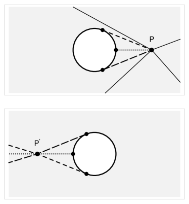
Figure 1: Geodesics emanating from point P in the “upper” universe of the vacuum-defect-wormhole spacetime with metric (11) and (14). Certain geodesics (thin solid lines) avoid the wormhole throat and stay in the upper universe, while other geodesics (heavy short-dashed/long-dashed/dotted lines) reach the wormhole throat (here shown as a thick circle with antipodal points identified) and cross over into the “lower” universe. The wormhole acts as a lens, with the transmitted geodesics refocussing at the point $\text{P}^{\,\prime}$ in the “lower” universe.

We have two further observations. First, recall that a permanent point-like source in Minkowski spacetime will, in principle, illuminate the whole of 3-space. But, in the vacuum-defect-wormhole spacetime, there will exist dark regions, even in the upper universe where the source is located. In the upper universe of Fig. 1, there is indeed a dark (shadow) region behind the wormhole throat (which has drained away some of the light emitted by the source). It is a straightforward exercise to describe the dark regions exactly.

Second, if the light source at P is no longer permanent but a flash instead, then we observe at $\text{P}^{\,\prime}$, after a certain moment, an expanding ring, even though there is no motion of the source position. This effect is entirely due to differences in the time-of-flight, for example, the time-of-flight of the short-dashed geodesic in Fig. 1 is larger than that of the dotted geodesic. The maximal angular extension ($2\alpha$) of the expanding ring and the source-observer distance ($D_{\,\text{PP}^{\prime}}$) can, in principle, give the vacuum-defect-wormhole length scale $\lambda$ by the expression (21).

Appendix B Preliminary numerical results

In the general Ansatz (11) for the defect-wormhole metric, we set

$$\widetilde{\phi}(\xi) = f(\xi)\,,$$ (22a)

$$\widetilde{r}^{\;2}(\xi) = \lambda^{2}+\xi^{2}+g(\xi)\,,$$ (22b)

so that a nonzero function $g(\xi)$ signals a non-vacuum wormhole configuration. For the numerical analysis, it turns out to be useful to compactify the quasi-radial $\xi$ coordinate,

$$\eta=\text{sgn}(\xi)\;\frac{\xi^{2}}{\lambda^{2}+\xi^{2}}\in[-1,\,1]\,.$$ (23)

In the following, we consider only nonnegative $\eta$ and $\xi$.

Next, we expand the metric functions $\overline{f}(\eta)=f(\xi)$ and $\overline{g}(\eta)=g(\xi)$ over $\eta\in[0,\,1]$,

$$\overline{f}(\eta) = \sum_{n=1}^{N_{f}}\,c_{n}\,\sin\big{(}n\,\pi\,\eta\big{)}\,,$$ (24a)

$$\overline{g}(\eta) = d_{0}\,(1-\eta)+\sum_{n=1}^{N_{g}}\,d_{n}\,\sin\big{(}n\,\pi\,\eta\big{)}\,,$$ (24b)

with finite cutoffs $N_{f}$ and $N_{g}$ on the sums. In this appendix, we take

$$\lambda=1\,,\quad d_{0}=1/10\,,$$ (25)

where the small but nonzero ratio $d_{0}/\lambda^{2}$ quantifies the deviation of the vacuum configuration.

Consider the radial null vector $\widehat{k}_{\,\mu}$ $=$ $\big{(}\exp\big{[}\,\overline{f}(\eta)\big{]},\,\sqrt{|\eta|},\,0,\,0\big{)}$ and the tangential null vector $\overline{k}_{\,\mu}$ $=$ $\big{(}\exp\big{[}\,\overline{f}(\eta)\big{]},\,0,\,\sqrt{\widetilde{r}^{\>2}},\,0\big{)}$, with replacement (22b) in terms of $\eta$. Then define the following quantities:

$$\Theta_{\text{rad}}\equiv G^{\,\mu}_{\;\;\,\nu}\,\widehat{k}_{\mu}\,\widehat{k}^{\,\nu}\,,$$ (26a)

$$\Theta_{\text{tang}}\equiv G^{\,\mu}_{\;\;\,\nu}\,\overline{k}_{\mu}\,\overline{k}^{\,\nu}\,,$$ (26b)

where $G^{\,\mu}_{\;\;\,\nu}\equiv R^{\,\mu}_{\;\;\,\nu}-{\textstyle\frac{1}{2}}\,g^{\,\mu}_{\;\;\,\nu}\,R$ is the Einstein tensor, which equals the energy-momentum tensor $T^{\,\mu}_{\;\;\,\nu}$ from the assumed validity of the Einstein equation for units with $8\pi G=1$.

We, now, introduce the following “penalty” measure:

$$\mathcal{P}\equiv\int_{0}^{1}\,d\eta\,\left(\Bigg{[}\sqrt{(\Theta_{\text{rad}})^{2}}-\Theta_{\text{rad}}\,\Bigg{]}^{2}+\Bigg{[}\sqrt{(\Theta_{\text{tang}})^{2}}-\Theta_{\text{tang}}\,\Bigg{]}^{2}\,\right)\,.$$ (27)

The Null Energy Condition (NEC), as discussed in Sec. II, gives $\mathcal{P}=0$. With the ad hoc expansion (24), the quantity $\mathcal{P}$ from (27) is a function of the coefficients $c_{n}$ and $d_{n}$, which can be minimized numerically. We have used the NMinimize routine of Mathematica 5.0.

With the eight coefficients from Table 1, we are able to reduce the penalty $\mathcal{P}$ to a value of order $10^{-5}$ and the corresponding results are shown in Fig. 2. Even more important than this small number for $\mathcal{P}$ is the fact that we have established a trend of dropping $\mathcal{P}$ for an increasing number of coefficients, as shown in Figs. 3 and 4. Observe also that the function shapes of $\overline{f}(\eta)$ and $\overline{g}(\eta)$ for $N_{\text{coeff}}\equiv N_{f}+N_{g}=4,\,6,\,8$ in Figs. 3 and 4 are more or less stable and that the absolute values of the the coefficients $c_{n}$ and $d_{n}$ in Table 1 drop for increasing order $n$. All this suggests that the numerical results converge on a nontrivial configuration, but this needs to be established rigorously.

Table 1: Eight nonzero coefficients giving $\mathcal{P}=1.72084\times 10^{-5}$, for numerical parameters $\lambda=1$ and $d_{0}=1/10$. The coefficients shown are exact numbers and can also be written as rational numbers, for example $d_{1}=152362/10^{6}$.

$\hskip 28.45274ptc_{1}=-0.0781046$	$d_{1}=\phantom{+}0.152362\hskip 28.45274pt$
$\hskip 28.45274ptc_{2}=\phantom{+}0.00959397$	$d_{2}=-0.0319350\hskip 28.45274pt$
$\hskip 28.45274ptc_{3}=-0.00560390$	$d_{3}=\phantom{+}0.0125051\hskip 28.45274pt$
$\hskip 28.45274ptc_{4}=\phantom{+}0.00491741$	$d_{4}=-0.00533132\hskip 28.45274pt$

The numerical results as they stand appear to indicate that

1. the obtained wormhole throat is larger than the one of the original (harvested) vacuum-defect wormhole, $\min_{\xi}\big{[}\widetilde{r}^{\;2}(\xi)\big{]}>\lambda^{2}$ ;

2. the energy density $\rho$ and the pressures $\{p_{\text{rad}},\,p_{\text{tang}}\}$ go to zero as $\xi^{-4}$ asymptotically;

3. there is only a small violation of the NEC far away from the wormhole throat [this NEC violation can be expected to vanish for an infinite number of appropriate coefficients and the resulting energy density $\rho(\eta)$ is perhaps nonnegative everywhere].

If these preliminary numerical results are confirmed, this implies that we can, in principle, widen the throat of a harvested vacuum-defect wormhole by adding a finite amount of non-exotic matter.

Addendum — Using an adapted penalty function $\mathcal{P}_{\text{NEW}}$ and the NMinimize routine of Mathematica 12.1, we have obtained $N_{\text{coeff}}=12$ metric functions (24) with a penalty value $\mathcal{P}\approx 6.1\times 10^{-6}$. The corresponding plots are similar to those of Fig. 2, but here we only show Fig 5 as a continuation of the sequence in Figs. 3 and 4.

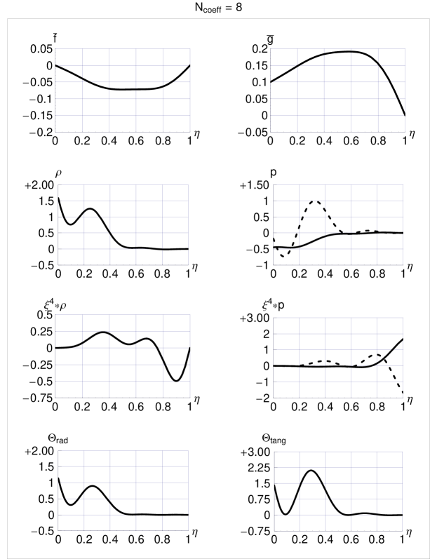
Figure 2: Metric Ansatz functions $\overline{f}(\eta)=f(\xi)$ and $\overline{g}(\eta)=g(\xi)$ in the metric (11) as defined by (22), (23), and (24) for the eight coefficients from Table 1, giving for the penalty function $\mathcal{P}$ from (27) the value $1.72084\times 10^{-5}$. In addition, there are the following numerical parameters: $\lambda=1$ and $d_{0}=1/10$. Several quantities result from the basic functions $\overline{f}(\eta)$ and $\overline{g}(\eta)$. The second row shows, at the left, the energy density $\rho\equiv G^{\,t}_{\;\;\,t}$ and, at the right, the pressures $p_{\text{rad}}\equiv G^{\,\xi}_{\;\;\,\xi}$ [solid curve] and $p_{\text{tang}}\equiv G^{\,\theta}_{\;\;\,\theta}$ [dashed curve], where $G^{\,\mu}_{\;\;\,\nu}$ is the Einstein tensor. On the third row, these last three quantities have been multiplied by $\xi^{4}=[\lambda^{2}\,\eta/(1-\eta)]^{2}$, in order to display their rapid asymptotic decrease (approximately as $\xi^{-4}$ for $\xi\to\infty$ or $\eta\to 1$). The fourth row shows the quantities $\Theta_{\text{rad}}$ and $\Theta_{\text{tang}}$ as defined by (26). The Null Energy Condition would correspond to having $\Theta_{\text{rad}}\geq 0$ and $\Theta_{\text{tang}}\geq 0$. With only eight coefficients, there are still small Null-Energy-Condition violations of $\Theta_{\text{rad}}$ at $\eta\sim 0.8$ and $\Theta_{\text{tang}}$ at $\eta\sim 0.9$; see the main text in App. B for further discussion.

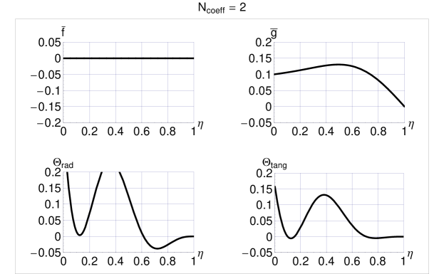
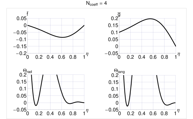
Figure 3: Numerical results for $N_{\text{coeff}}\equiv N_{f}+N_{g}=2$ in the top panel [penalty $\mathcal{P}=0.000812553$ for nonzero coefficients $d_{1}=0.0805092$ and $d_{2}=-0.0151493$] and for $N_{\text{coeff}}=4$ in the bottom panel [penalty $\mathcal{P}=0.000111302$ for nonzero coefficients $c_{1}=-0.0789967$, $c_{2}=0.0186060$, $d_{1}=0.144524$, and $d_{2}=-0.0286358$].

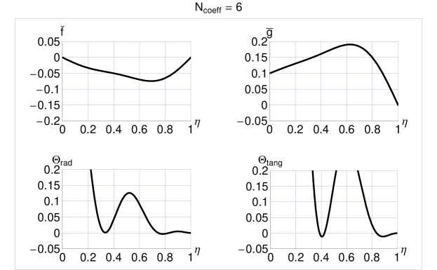
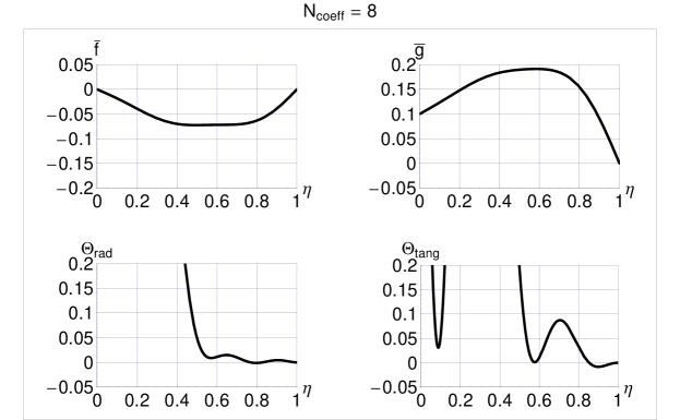
Figure 4: Numerical results for $N_{\text{coeff}}=6$ in the top panel [penalty $\mathcal{P}=0.0000316721$ for nonzero coefficients $c_{1}=-0.0686991$, $c_{2}=0.0168485$, $c_{3}=-0.00924705$, $d_{1}=0.137967$, $d_{2}=-0.0416794$, and $d_{3}=0.00952128$] and for $N_{\text{coeff}}=8$ in the bottom panel [penalty $\mathcal{P}=0.0000172084$ for the nonzero coefficients from Table 1 ]. For $N_{\text{coeff}}=8$, the $\Theta_{\text{rad}}$ value drops to approximately $-0.001$ at $\eta\sim 0.8$ and the $\Theta_{\text{tang}}$ value to approximately $-0.01$ at $\eta\sim 0.9$.

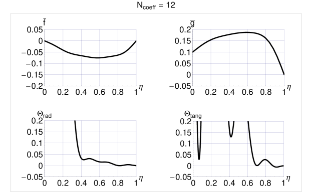
Figure 5: Numerical results for $N_{\text{coeff}}=12$ with $\mathcal{P}=6.12347\times 10^{-6}$ for nonzero coefficients $c_{1}=-0.0782196$, $c_{2}=0.0107336$, $c_{3}=-0.00647395$, $c_{4}=0.00391987$, $c_{5}=-0.00119384$, $c_{6}=0.00229041$ and $d_{1}=0.151704$, $d_{2}=-0.0321288$, $d_{3}=0.0195948$, $d_{4}=-0.00525931$, $d_{5}=0.00290803$, $d_{6}=-0.000818478$. The $\Theta_{\text{rad}}$ value drops to approximately $-5\times 10^{-5}$ at $\eta\sim 0.8$ and the $\Theta_{\text{tang}}$ value to approximately $-5\times 10^{-3}$ at $\eta\sim 0.9$.

References

- (1) M.S. Morris and K.S. Thorne, “Wormholes in space-time and their use for interstellar travel: A tool for teaching general relativity,” Am. J. Phys. 56, 395 (1988).
- (2) M. Visser, Lorentzian Wormholes: From Einstein to Hawking (Springer, New York, NY, 1996).
- (3) F.R. Klinkhamer, “Regularized big bang singularity,” Phys. Rev. D 100, 023536 (2019), arXiv:1903.10450.
- (4) F.R. Klinkhamer, “More on the regularized big bang singularity,” Phys. Rev. D 101, 064029 (2020), arXiv:1907.06547.
- (5) F.R. Klinkhamer and Z.L. Wang, “Nonsingular bouncing cosmology from general relativity,” Phys. Rev. D 100, 083534 (2019), arXiv:1904.09961.
- (6) F.R. Klinkhamer and Z.L. Wang, “Nonsingular bouncing cosmology from general relativity: Scalar metric perturbations,” Phys. Rev. D 101, 064061 (2020), arXiv:1911.06173.
- (7) F.R. Klinkhamer, “M-theory and the birth of the Universe,” Acta Phys. Polon. B 52, 1007 (2021), arXiv:2102.11202.
- (8) H.G. Ellis, “Ether flow through a drainhole: A particle model in general relativity,” J. Math. Phys. 14, 104 (1973); Errata J. Math. Phys. 15, 520 (1974).
- (9) K.A. Bronnikov, “Scalar-tensor theory and scalar charge,” Acta Phys. Polon. B 4, 251 (1973).
- (10) T. Eguchi, P.B. Gilkey, and A.J. Hanson, “Gravitation, gauge theories and differential geometry,” Phys. Rept. 66, 213 (1980).
- (11) M. Nakahara, Geometry, Topology and Physics, Second Edition (Institute of Physics Publ., Bristol, UK, 2003).
- (12) F.R. Klinkhamer, “Skyrmion spacetime defect,” Phys. Rev. D 90, 024007 (2014), arXiv:1402.7048.
- (13) F.R. Klinkhamer and F. Sorba, “Comparison of spacetime defects which are homeomorphic but not diffeomorphic,” J. Math. Phys. 55, 112503 (2014), arXiv:1404.2901.
-
(14)
M. Guenther,
“Skyrmion spacetime defect, degenerate metric, and negative gravitational mass,”
Master Thesis, KIT, September 2017;
available from
https://www.itp.kit.edu/en/publications/diploma - (15) F.R. Klinkhamer, “On a soliton-type spacetime defect,” J. Phys. Conf. Ser. 1275, 012012 (2019), arXiv:1811.01078.
- (16) F.R. Klinkhamer, “A new type of nonsingular black-hole solution in general relativity,” Mod. Phys. Lett. A 29, 1430018 (2014), arXiv:1309.7011.
- (17) F.R. Klinkhamer and Z.L. Wang, “Lensing and imaging by a stealth defect of spacetime,” Mod. Phys. Lett. A 34, 1950026 (2019), arXiv:1808.02465.
- (18) G.T. Horowitz, “Topology change in classical and quantum gravity,” Class. Quant. Grav. 8, 587 (1991).
- (19) M. Calzà, M. Rinaldi, and L. Sebastiani, “A special class of solutions in -gravity,” Eur. Phys. J. C 78, 178 (2018), arXiv:1802.00329.
- (20) S. Kar, S. Lahiri, and S. SenGupta, “Can extra dimensional effects allow wormholes without exotic matter?,” Phys. Lett. B 750, 319 (2015), arXiv:1505.06831.
- (21) R.A. Konoplya and A. Zhidenko, “Traversable wormholes in general relativity,” Phys. Rev. Lett. 128, 091104 (2022), arXiv:2106.05034.
- (22) D.R. Terno, “Inaccessibility of traversable wormholes,” Phys. Rev. D 106, 044035 (2022), arXiv:2203.03770.
- (23) S. Biswas, M. Rahman, and S. Chakraborty, “Echoes from braneworld wormholes,” Phys. Rev. D 106, 124003 (2022), arXiv:2205.14743.
- (24) N. Ishibashi, H. Kawai, Y. Kitazawa, and A. Tsuchiya, “A large- reduced model as superstring,” Nucl. Phys. B 498, 467 (1997), arXiv:hep-th/9612115.
- (25) H. Aoki, S. Iso, H. Kawai, Y. Kitazawa, A. Tsuchiya, and T. Tada, “IIB matrix model,” Prog. Theor. Phys. Suppl. 134, 47 (1999), arXiv:hep-th/9908038.
- (26) F.R. Klinkhamer, “IIB matrix model: Emergent spacetime from the master field,” Prog. Theor. Exp. Phys. 2021, 013B04 (2021), arXiv:2007.08485.
- (27) F.R. Klinkhamer, “IIB matrix model and regularized big bang,” Prog. Theor. Exp. Phys. 2021, 063B05 (2021), arXiv:2009.06525.
- (28) F.R. Klinkhamer, “Vacuum defect wormholes and a mirror world,” arXiv:2305.13278.
- (29) L. Chetouani and G. Clément, “Geometrical optics in the Ellis geometry,” Gen. Rel. Grav. 16, 111 (1984).
- (30) V. Perlick, “On the exact gravitational lens equation in spherically symmetric and static space-times,” Phys. Rev. D 69, 064017 (2004), arXiv:gr-qc/0307072.
- (31) K.K. Nandi, Y.Z. Zhang, and A.V. Zakharov, “Gravitational lensing by wormholes,” Phys. Rev. D 74, 024020 (2006), arXiv:gr-qc/0602062.
- (32) N. Tsukamoto and T. Harada, “Light curves of light rays passing through a wormhole,” Phys. Rev. D 95, 024030 (2017), arXiv:1607.01120.
- (33) R. Shaikh, P. Banerjee, S. Paul, and T. Sarkar, “A novel gravitational lensing feature by wormholes,” Phys. Lett. B 789, 270 (2019) [erratum: Phys. Lett. B 791, 422 (2019)], arXiv:1811.08245.