Complete analysis on QED corrections to $B_{q}\,\to\,\tau^{+}\,\tau^{-}$

Abstract

Motivated by a dynamical enhancement of the electromagnetic corrections by a power of $\Lambda_{\mathrm{QCD}}/m_{b}$ in $B_{d,s}\,\to\,\mu^{+}\,\mu^{-}$ at next-to-leading order (NLO), we extend the QED factorization effects on the leptonic $B$ meson decays with light muon leptons to tauonic final states, $B_{d,s}\,\to\,\tau^{+}\,\tau^{-}$, using soft-collinear effective theory (SCET). This extension is necessary owing to the appearance of the large $\tau$ mass, which will lead to different power counting in SCET and also different results. We provide a complete NLO electromagnetic corrections to $B_{d,s}\,\to\,\tau^{+}\,\tau^{-}$, which include hard functions and hard-collinear functions below the bottom quark mass scale $\mu_{b}$. The power enhanced electromagnetic effects from hard-collinear contributions on $B_{d,s}\,\to\,\mu^{+}\,\mu^{-}$ discussed before also exist in $B_{d,s}\,\to\,\tau^{+}\,\tau^{-}$. However the logarithm term arising from contributions of hard-collinear photon and lepton virtualities for $B_{d,s}\,\to\,\tau^{+}\,\tau^{-}$ is not large as it is in muon case due to the hard-collinear scale of $\tau$ mass, which lead to only approximately $0.04\%$ QED corrections to the branching fraction of $B_{d,s}\,\to\,\tau^{+}\,\tau^{-}$ compared with overall reduction about $0.5\%$ in $B_{d,s}\,\to\,\mu^{+}\,\mu^{-}$.

1 Introduction

The purely leptonic decays $B_{q}\,\to\,\ell^{+}\,\ell^{-}$, with $q=d,\,s$ and $\ell=e,\mu,\tau$, are highly suppressed in the standard model (SM) due to the loop suppresses (FCNC) and helicity suppresses. Therefore, they have an important role in the study of physics beyond the Standard Model (BSM). They are also of interest owning to their clear theoretical descriptions. In fact, the only relevant quantity that needs to be calculated at the leading order of $\alpha_{\mathrm{em}}$ is $B$-meson decay constant $f_{B}$. The branching ratio of $B_{q}\,\to\,\ell^{+}\,\ell^{-}$ at the leading orders in flavor-changing weak interactions and in $m_{B_{q}}^{2}/m_{W}^{2}$ can be expressed as Bobeth:2013uxa ,

$${\mathcal{B}}\left[\,B_{q}\,\rightarrow\,\ell^{+}\,\ell^{-}\,\right]\,=\,\frac{|N|^{2}m_{B_{q}}^{3}\,f_{B_{q}}^{2}}{8\,\pi\,\Gamma_{H}^{q}}\,\beta_{q\ell}\,r_{q\ell}^{2}\,\left|C_{A}\left(\mu_{b}\right)\right|^{2}\,+\,\mathcal{O}\left(\alpha_{\mathrm{em}}\right)\,,$$ (1)

where $r_{q\ell}=2m_{\ell}/m_{B_{q}}$ and $\beta_{q\ell}=\sqrt{1-r_{q\ell}^{2}}$. The normalization constant $N=V_{tb}^{*}V_{tq}G_{F}^{2}m_{W}^{2}/\pi^{2}$ and $\Gamma_{H}^{q}$ denotes the heavier mass-eigenstate total width of $B_{q}-\bar{B}_{q}$ mixing. $C_{A}$ is the $\overline{\mathrm{MS}}$-renormalized Wilson coefficient associated with the operator $\left[\,\bar{b}\,\gamma_{\alpha}\,\gamma_{5}\,q\,\right]\,\left[\,\bar{\ell}\,\gamma^{\alpha}\,\gamma_{5}\,\ell\,\right]$ at the scale $\mu_{b}$. Up to date, the most precise determinations of $f_{B_{u,d}}$ and $f_{B_{s}}$ have already reached the relative precision of about $0.7\%$ and $0.5\%$ from lattice QCD, respectively Bazavov:2017lyh . These precise values of $f_{B}$ from lattice calculations provide a motivation for improving the perturbative ingredients which arise from several energy scales spanned by the SM. The QCD corrections to $C_{A}$ have been up to the next-to-next-to-leading order (NNLO) Hermann:2013kca . At the scale $\mu\,\geq\,\mu_{b}$, the electroweak (EW) corrections at NLO have been done in Bobeth:2013tba , which combined with NNLO QCD corrections are calculated in Bobeth:2013uxa . In recent years, a consistent simultaneous treatment of QCD and QED corrections to $B_{q}\,\to\,\mu^{+}\,\mu^{-}$ below scale $\mu_{b}$ have been finished in Beneke:2017vpq ; Beneke:2019slt .

As far as the $\mathcal{O}\left(\alpha_{\mathrm{em}}\right)$ term in Eq.(1) is concerned, M. Benenke et al. found that QED virtual photon exchanged between one of the final-state leptons and the light spectator antiquark $\bar{q}$ in the $\bar{B}_{q}$ meson could effectively probe the $\bar{B}_{q}$ meson structure, resulting in a “non-local annihilation” effect for muon leptonic $\bar{B}_{q}$ meson decays Beneke:2017vpq ; Beneke:2019slt ; Feldmann:2022ixt . The spectator-$b$-quark annihilation over the distance $1/\sqrt{m_{B}\,\Lambda_{\mathrm{QCD}}}$ inside the $\bar{B}_{q}$ meson causes the strong interaction effects no longer to be parameterized by $f_{B}$ alone and provides approximately $1\%$ power-enhancement on branching ratio of $B_{q}\,\to\,\mu^{+}\,\mu^{-}$. This power-enhanced QED effect is substantially large and is in fact of the same order as the non-parametric theoretical uncertainty (about $1.5\%$ Bobeth:2013uxa ). Eventually, the theoretical uncertainty of the prediction on the decay $B_{s}\,\to\,\mu^{+}\,\mu^{-}$ is reduced largely, which will be necessary for matching the experimental accuracy with higher experimental statistics by LHCb and Belle II in the future. Recently, in Cornella:2022ubo , M. Neubert et al. considered the virtual QED corrections though the process $B^{-}\,\to\,\mu^{-}\,\bar{\nu}_{\mu}$ to further probe the internal structure of the $B$-meson at subleading power in $\Lambda_{\mathrm{QCD}}/m_{B}$.

In view of the novel QED effect on $B_{q}\,\to\,\mu^{+}\,\mu^{-}$ below $\mu_{b}$ scale, it would be desirable to study the other leptonic final states $\ell=e,\,\tau$ as QED corrections on these decays below $\mu_{b}$ scale will be process dependence. The muon mass is numerically of the order of the strong interaction scale $\Lambda_{\mathrm{QCD}}$, while the much smaller electron mass, and especially the much larger mass of the tau lepton imply that the results of $B_{q}\,\to\,e^{+}\,e^{-}$ and $B_{q}\,\to\,\tau^{+}\,\tau^{-}$ are not just trival generations from the case $\ell=\mu$ discussed above. In this work, we will focus on $\tau$ leptonic final states, $B_{q}\,\to\,\tau^{+}\,\tau^{-}$. As the branching ratio depends strongly on lepton mass due to helicity suppression, tau leptonic $B$-meson decay is expected to have the largest leptonic branching fraction. However, the experimental picture for the tau channel is complicated. The necessity to reconstruct the tau lepton from its decay products in the presence of two or three undetectable neutrinos make the background rejection an experimental challenge. The modes of $B_{q}\,\to\,\tau^{+}\,\tau^{-}$ have not yet been experimentally observed to date. The measurements of $B_{q}\,\to\,\tau^{+}\,\tau^{-}$ at LHCb yield an upper limit for their branching ratios, $\mathcal{B}\left(B^{0}\,\rightarrow\,\tau^{+}\,\tau^{-}\right)\,<\,2.1\,\times\,10^{-3}$ LHCb:2017myy and $\mathcal{B}\left(B_{s}^{0}\,\rightarrow\,\tau^{+}\,\tau^{-}\right)\,<\,5\,\times\,10^{-4}$ LHCb:2018roe . Nevertheless, they are expected to be improved by experiments, such as Belle II Belle-II:2018jsg and LHCb Upgrade II LHCb:2018roe , within the next few years. On the theoretical side, we will present an extension of the previous formulation in the context of SCET for muon leptonic $B$-meson decays to tau final states. A new element is the appearance of the order of hard-collinear scale $m_{b}\,\Lambda_{\mathrm{QCD}}$ ($m_{\tau}^{2}\,\sim\,m_{b}\,\Lambda_{\mathrm{QCD}}$) in the final states, which will be integrated out and the $\tau$ leptonic field then becomes a soft-collinear field described by boosted heavy lepton effective theory (bHLET), similarly to the boosted HQET Fleming:2007qr ; Fleming:2007xt , not a collinear mode in $\mathrm{SCET_{II}}$ as for muon final state. It naturally makes the applications of SCET for $B_{q}\,\to\,\tau^{+}\,\tau^{-}$ different from the case of $B_{q}\,\to\,\mu^{+}\,\mu^{-}$. We will do two-step matching starting from $\mathrm{QCD}\times\mathrm{QED}$ onto $\mathrm{SCET_{I}}$, and successively onto $\mathrm{HQET}\times\mathrm{bHLET}$, rather than $\mathrm{SCET_{II}}$ as in muon case. Hard-collinear functions derived from the matching, $\mathrm{SCET_{I}}\,\to\,\mathrm{HQET}\times\mathrm{bHLET}$, will be formally response to the power enhancement term $m_{b}/\Lambda_{\mathrm{QCD}}$. However the logarithm term arising from the contributions of hard-collinear photon and lepton virtualities in the hard-collinear functions is not large for $B_{q}\,\to\,\tau^{+}\,\tau^{-}$ as the tau mass is just the order of hard-collinear scale, which would not lead to a large enhanced QED effect even though the same power enhancement by a factor $m_{b}/\Lambda_{\mathrm{QCD}}$ appears in $B_{q}\,\to\,\tau^{+}\,\tau^{-}$. In addition to the hard-collinear corrections, one-loop hard functions will also been extracted in the first-step matching, $\mathrm{QCD}\times\mathrm{QED}\to\mathrm{SCET_{I}}$, for a complete QED correction to leptonic $B$-meson decays. At last, the renormalizations of $B_{q}\,\to\,\tau^{+}\,\tau^{-}$ will be a simple generation from $B_{q}\,\to\,\mu^{+}\,\mu^{-}$.

The remainder of this paper is organized as follows: In Sec. 2, we briefly introduce the conventions for effective weak interactions for $b\,\rightarrow\,q\,\ell^{+}\,\ell^{-}$. The fields and their power counting relevant to $B_{q}\,\to\,\tau^{+}\,\tau^{-}$ are discussed in Sec. 3.1. We detail the decoupling of hard virtualities in $\mathrm{SCET_{I}}$ and further the one of hard-collinear virtualities in $\mathrm{HQET}\times\mathrm{bHLET}$ in Sec. 3.2 and Sec. 3.3, respectively. Successively, in Sec. 3.4, matrix element of soft function in $\mathrm{HQET}\times\mathrm{bHLET}$ is presented. The RG evolutions involving hard functions and soft functions are left to Sec. 4. The decay widths of $B_{q}\,\to\,\tau^{+}\,\tau^{-}$ together with the ultrasoft parts are given in Sec. 5. We proceed with the numerical impact of QED corrections to $B_{q}\,\to\,\tau^{+}\,\tau^{-}$ in Sec. 6. Eventually, we summarize in Sec. 7.

2 Effective Weak Interactions for $b\,\rightarrow q\,\ell^{+}\,\ell^{-}$

We start by discussing briefly the effective weak interactions for $b\,\rightarrow q\,\ell^{+}\,\ell^{-}$, with $\ell=e\,,\mu\,,\tau$. They can be firstly derived from the SM by decoupling the top quark, the Higgs boson, and the heavy electroweak bosons W and Z. Then the operator product expansion (OPE) for this effective Lagrangian relevant for $|\Delta B|\,=\,1$ decays $b\,\rightarrow\,q\,\ell^{+}\,\ell^{-}$ with $q=d,\,s$ reads

$$\mathcal{L}_{\Delta B=1}\,=\,\mathcal{N}_{\Delta B=1}\,\left[\,\sum_{i=1}^{10}\,C_{i}\left(\mu_{b}\right)\,Q_{i}\,+\,\frac{V_{ub}\,V_{uq}^{*}}{V_{tb}\,V_{tq}^{*}}\,\sum_{i=1}^{2}\,C_{i}\left(\mu_{b}\right)\,\left(Q_{i}^{c}\,-\,Q_{i}^{u}\right)\,\right]\,+\,\mathrm{h.c.}\,,$$ (2)

where the effective operators $Q_{i}$ are current-current operators $(i\,=\,1,\,2)$, QCD-penguin operators $(i\,=\,$ $\,3,\,\ldots,\,6)$, dipole operators $(i\,=\,7,\,8)$ and semileptonic operators $(i\,=\,9,\,10)$. Here we only list those of the three most relevant operators, which followed the operator definitions of Ref. Chetyrkin:1996vx ,

$$Q_{7} \,=\,\frac{e}{(4\,\pi)^{2}}\,\overline{m}_{b}\,\left[\,\bar{q}\,\sigma^{\mu\nu}\,P_{R}\,b\,\right]\,F_{\mu\nu}\,,$$ (3)

$$Q_{9} \,=\,\frac{\alpha_{\mathrm{em}}}{4\,\pi}\,\left(\bar{q}\,\gamma^{\mu}\,P_{L}\,b\,\right)\,\sum_{\ell}\,\bar{\ell}\,\gamma_{\mu}\,\ell\,,$$ (4)

$$Q_{10} \,=\,\frac{\alpha_{\mathrm{em}}}{4\,\pi}\,\left(\bar{q}\,\gamma^{\mu}\,P_{L}\,b\right)\,\sum_{\ell}\,\bar{\ell}\,\gamma_{\mu}\,\gamma_{5}\,\ell\,,$$ (5)

where $\overline{m}_{b}$ represents the running $b$-quark mass in the $\overline{\mathrm{MS}}$ subtraction scheme. The normalization constant, $\mathcal{N}_{\Delta B=1}\,\equiv\,2\,\sqrt{2}\,G_{F}\,V_{tb}\,V_{ts}^{*}$, is given in terms of the Fermi constant and the Cabibbo-Kobayashi-Maskawa (CKM) matrix elements. $C_{i}\left(\mu_{b}\right)$ denotes the $\overline{\mathrm{MS}}$-renormalized Wilson coefficient at the scale $\mu_{b}\,\sim\,m_{b}$. The matching coefficients of all of those operators at the electroweak scale $\mu_{W}\,\sim\,m_{W}$ of the order of the $W$-boson mass have been up to the precise of NNLO in QCD Hermann:2013kca ; Bobeth:1999mk and further $C_{10}$ includes NLO EW corrections Bobeth:2013tba . The scale running of $C_{i}\left(\mu\right)$ from the scale $\mu_{W}$ to $\mu_{b}$ has been taken into account in Bobeth:2013tba ; Bobeth:2003at ; Huber:2005ig ; Huber:2019iqf ; Huber:2020vup , and the numerical values of $C_{i}\left(\mu_{b}\right)$ will be given in Section 6.

3 Factorization in $B_{q}\,\rightarrow\,\ell^{+}\,\ell^{-}$ decay below the scale $m_{b}$

The heavy-quark systems $B_{q}$ can be described well by heavy-quark effective theory (HQET) Georgi:1990um . The process $B_{q}\,\rightarrow\,\ell^{+}\,\ell^{-}$ also involves final energetic light particles where some components of their momentas $p_{\mu}$ are large, but their $p^{2}$ are small when compared with the heavy $B$-meson. More specifically, working in the rest frame of the initial $B$-meson and choosing the $z$-direction as the direction of the one of the two leptons, their momentas can be written as

$$\begin{aligned} p_{\ell^{+}}^{\mu}&\,=\,(E_{\ell^{+}},\,0,\,0,\,\sqrt{m_{B}^{2}\,-\,4\,m_{\ell}^{2}}/2)\,,\\ p_{\ell^{-}}^{\mu}&\,=\,(E_{\ell^{-}},\,0,\,0,\,-\sqrt{m_{B}^{2}\,-\,4\,m_{\ell}^{2}}/2)\,,\end{aligned}$$ (6)

where the large energies are $E_{\ell^{+}}\,=\,E_{\ell^{-}}\,=\,m_{B}/2$ and the final-state leptons are on-shell, $p_{\ell^{+}}^{2}\,=\,p_{\ell^{-}}^{2}\,=\,m_{\ell}^{2}$. The presence of several different scales in $B_{q}\,\rightarrow\,\ell^{+}\,\ell^{-}$ decay means that we can classify quantum fluctuations as hard, hard-collinear (collinear), or soft. For $\ell\,=\,\tau$, the corresponding scales are

$$\begin{aligned} \text{ hard: }&m_{B}\,,E_{\tau}\,,\\ \text{ hard-collinear: }&m_{\tau}\,\sim\,\sqrt{m_{B}\,\Lambda_{\mathrm{QCD}}}\,,\\ \text{ soft: }&\Lambda_{\mathrm{QCD}}\,.\end{aligned}$$ (7)

Our goal is to integrate out all short-distance scales including hard and hard-collinear quantum fluctuations. Therefore the construction of EFTs often proceeds two-step matching procedure: in the first step, hard quantum fluctuations are integrated out by matching the effective weak Lagrangian in Eq.(2) onto $\mathrm{SCET_{I}}$ with hard-collinear or soft momenta as dynamical degrees of freedom; in the second step, by matching $\mathrm{SCET_{I}}$ onto $\mathrm{HQET}\times\mathrm{bHLET}$, fluctuations at the hard-collinear scale are integrated out. The explicit factorizations of the two short-distance scales from long-distance scale will be done in the following two subsections.

3.1 Power Counting

In view of the presence of fast, hard-collinear final particles, it is convenient to decompose 4-vectors in a light-cone basis spanned by two light-like reference vectors $n_{+}^{\mu}$, $n_{-}^{\mu}$ and a remainder perpendicular to both. We often choose $n_{+}^{\mu}\,=\,(1,\,0,\,0,\,1)$ and $n_{-}^{\mu}\,=\,(1,\,0,\,0,\,-1)$ to make one of the two final states align along the $n_{+}^{\mu}$ direction, and the other point the opposite direction, $n_{-}^{\mu}$. An arbitrary vector $p^{\mu}$ can then be decomposed in a component proportional to $n_{+}^{\mu}$, a part proportional to $n_{-}^{\mu}$, and the transverse direction,

$$\begin{aligned} p^{\mu}&\,=\,(n_{+}p)\,\frac{n_{-}^{\mu}}{2}\,+\,(n_{-}p)\,\frac{n_{+}^{\mu}}{2}\,+\,p_{\perp}^{\mu}\\ &\,\equiv\,\left(n_{+}p\,,\,n_{-}p\,,\,p_{\perp}\right)\,.\end{aligned}$$ (8)

On the partonic level, $B_{q}\,\rightarrow\,\ell^{+}\,\ell^{-}$ decay processes as

$$b\left(p_{b}\right)\,+\,q\left(l_{q}\right)\,\rightarrow\,\ell^{+}\left(p_{\ell^{+}}\right)\,+\,\ell^{-}\left(p_{\ell^{-}}\right)\,.$$ (9)

The momentums of two final states are decomposed as

$$p_{\ell^{+}}^{\mu} \,=\,\frac{m_{B}\,-\,\sqrt{m_{B}^{2}\,-\,4\,m_{\ell}^{2}}}{2}\,\frac{n_{-}^{\mu}}{2}\,+\,\frac{m_{B}\,+\,\sqrt{m_{B}^{2}\,-\,4\,m_{\ell}^{2}}}{2}\,\frac{n_{+}^{\mu}}{2}\,,$$ (10)

$$p_{\ell^{-}}^{\mu} \,=\,\frac{m_{B}\,+\,\sqrt{m_{B}^{2}\,-\,4\,m_{\ell}^{2}}}{2}\,\frac{n_{-}^{\mu}}{2}\,+\,\frac{m_{B}\,-\,\sqrt{m_{B}^{2}\,-\,4\,m_{\ell}^{2}}}{2}\,\,\frac{n_{+}^{\mu}}{2}\,.$$ (11)

Specifically, for $\ell\,=\,\tau$, $n_{+}\,p_{\tau^{-}}\,=\,n_{-}\,p_{\tau^{+}}\,\sim\,m_{b}$ and $n_{-}\,p_{\tau^{-}}\,=\,n_{+}\,p_{\tau^{+}}\,\sim\,\Lambda_{\mathrm{QCD}}$. A softly interacting heavy $b$-quark is nearly on-shell with its momentum $p^{\mu}_{b}\,=\,m_{b}\,v^{\mu}\,+\,l_{b}^{\mu}\,$, where $v^{\mu}$ is the 4-velocity of the $B_{q}$ meson, $v^{\mu}=(n_{+}^{\mu}+n_{-}^{\mu})/2$, and the “residual momentum” $l_{b}\,\sim\Lambda_{\mathrm{QCD}}$. Also the momentum of light spectator quark is $l_{q}\,\sim\,\Lambda_{\mathrm{QCD}}$.

Besides the external kinematics above for $B_{q}\,\rightarrow\,\tau^{+}\,\tau^{-}$ decay, the internal dynamic momentum, denoted by $k^{\mu}$, can be classified according to their scaling properties with $m_{b}\,\gg\,\Lambda_{\mathrm{QCD}}$ as

$$\begin{aligned} \text{ hard: }&\,k_{h}^{\mu}\,=\,m_{b}\,(1,\,1,\,1)\sim(1,\,1,\,1)\,,\\ \text{ hard-collinear: }&\,k_{hc}^{\mu}\,=\,(m_{b},\,\Lambda_{\mathrm{QCD}},\,\sqrt{m_{b}\,\Lambda_{\mathrm{QCD}}})\,\sim\,(1,\,\lambda^{2},\,\lambda)\,,\\ \text{anti-hard-collinear: }&\,k_{\overline{hc}}^{\mu}\,=\,(\Lambda_{\mathrm{QCD}},\,m_{b},\,\sqrt{m_{b}\,\Lambda_{\mathrm{QCD}}})\,\sim\,(\lambda^{2},\,1,\,\lambda)\,,\\ \text{ soft: }&\,k_{s}^{\mu}\,=\,(\Lambda_{\mathrm{QCD}},\,\Lambda_{\mathrm{QCD}},\,\Lambda_{\mathrm{QCD}})\,\sim\,(\lambda^{2},\,\lambda^{2},\,\lambda^{2})\,,\\ \text{ soft-collinear: }&\,k_{sc}^{\mu}\,=\,(1/b,\,b,\,1)\,\Lambda_{\mathrm{QCD}},\,\sim\,(1/b,\,b,\,1)\,\lambda^{2}\,,\\ \text{ anti-soft-collinear: }&\,k_{sc}^{\mu}\,=\,(b,\,1/b,\,1)\,\Lambda_{\mathrm{QCD}},\,\sim\,(b,\,1/b,\,1)\,\lambda^{2}\,,\end{aligned}$$ (12)

with scaling parameter $\lambda^{2}\,=\,\Lambda_{\mathrm{QCD}}/m_{b}$ and the boosted parameter $b=m_{\tau}/m_{b}$. The corresponding virtualities are $k_{h}^{2}\,\sim\,m_{b}^{2}$, $k_{hc}^{2}\,=\,k_{\overline{hc}}^{2}\,\sim\,m_{b}\,\Lambda_{\mathrm{QCD}}$, and $k_{s}^{2}\,\sim\,\Lambda_{\mathrm{QCD}}^{2}$. Different from the light final particles $\ell\,=\,\mu$, collinear virtuality $k_{c}^{2}\,\sim\,\Lambda_{\mathrm{QCD}}^{2}$ does not appear in massive $\tau$ lepton case ($m_{\tau}^{2}\,\sim\,m_{b}\,\Lambda_{\mathrm{QCD}}$). The massive $\tau$ field will be integrated out and become a soft-collinear field in bHLET. Consequently, the matching procedure of EFTs would also be different from $B_{d,s}\to\mu^{+}\mu^{-}$. As mentioned above, after integrating out hard modes (i.e., $k_{h}^{2}\,\sim\,m_{b}^{2}$), we obtain the $\mathrm{SCET_{I}}$ including the (anti-)hard-collinear and soft (soft-collinear) modes. Subsequently, the (anti-)hard-collinear modes of light quark (i.e., $k_{hc}^{2}\,=\,k_{\overline{hc}}^{2}\,\sim\,m_{b}\,\Lambda_{\mathrm{QCD}}$) will be integrated out to become the soft field in HQET, but the (anti-)hard-collinear $\tau$ field will be turned to be the (anti-)soft-collinear field after integrating out the mass of $\tau$ lepton in bHLET. The matching procedure simply follows as

full QED $$\to {}_{\text{I}} \hskip-17.07182pt\to\hskip 42.67912pt\text{$\mathrm{HQET}\times\mathrm{bHLET}$}$$ SCET

$$\text{hard:}\;\mu_{h}^{2}\sim m_{b}^{2} \;\mu_{hc}^{2}\sim m_{b}\Lambda_{\mathrm{QCD}} \text{soft(-collinear):}\;\mu_{s(c)}^{2}\sim\Lambda_{\mathrm{QCD}}^{2}$$ hard-collinear:

At last, we introduce various fields of SCET${}_{\text{I}}$ and $\mathrm{HQET}\times\mathrm{bHLET}$ obtained by decomposing the quark, lepton and photon (gluon) fields into various momentum modes. The fields and their scalings are

$$\begin{aligned} \text{soft heavy quark:}&\quad h_{v}\,\sim\,\lambda^{3}\,,\\ \text{hard-collinear light quark:}&\quad\chi_{hc}\,\sim\,\lambda\,,\\ \text{hard-collinear leptonic field:}&\quad\ell_{hc}\,\sim\,\lambda\,,\\ \text{soft light quark:}&\quad q_{s}\,\sim\,\lambda^{3}\,,\\ \text{soft-collinear leptonic field:}&\quad\ell_{sc}\,\sim\,\lambda^{3}\,,\\ \text{hard-collinear photon\, (gluon):}&\quad A_{hc}^{\mu}(G_{hc}^{\mu})\,\sim\,(1,\,\lambda^{2},\,\lambda)\,,\\ \text{soft photon\, (gluon):}&\quad A_{s}^{\mu}(G_{s}^{\mu})\,\sim\,\lambda^{2}\,(1,\,1,\,1)\,.\end{aligned}$$ (13)

3.2 $\mathrm{SCET_{I}}$

In this subsection, we will present the effective operators in $\mathrm{SCET_{I}}$ and hard fluctuations decoupled in the matching of weak EFT onto $\mathrm{SCET_{I}}$ up to NLO.

3.2.1 Operators

After introducing the relevant fields and discussing their power counting, we proceeded to present $\mathrm{SCET_{I}}$ operators in the matching of the effective weak Hamiltonian to $\mathrm{SCET_{I}}$. As the $\mathrm{SCET_{I}}$ operators for $B_{q}\,\to\,\tau^{+}\,\tau^{-}$ decay are the same as in $\mu$ leptonic decay Beneke:2019slt , we just list those operators here and the details of their constructions can be found in the Appendix of that paper Beneke:2019slt and earlier works Beneke:2003pa ; Beneke:2017ztn . With the power counting of fields in Eq.(13), the smallest $\lambda$ scaling of $\mathrm{SCET_{I}}$ operators relevant to the matching of effective operators $Q_{9,10}$ are order of $\lambda^{6}$. In the coordinate-space, labelled by a tilde, they are

$$\widetilde{\mathcal{O}}_{9}(s,t) \,=\,g_{\mu\nu}^{\perp}\,\left[\,\bar{\chi}_{hc}\left(sn_{+}\right)\,\gamma_{\perp}^{\mu}\,P_{L}\,h_{v}(0)\,\right]\,\left[\,\bar{\ell}_{hc}\left(tn_{+}\right)\,\gamma_{\perp}^{\nu}\,\ell_{\overline{hc}}(0)\,\right]\,,$$ (14)

$$\widetilde{\mathcal{O}}_{10}(s,t) \,=\,i\varepsilon_{\mu\nu}^{\perp}\,\left[\,\bar{\chi}_{hc}\left(sn_{+}\right)\,\gamma_{\perp}^{\mu}\,P_{L}\,h_{v}(0)\,\right]\left[\,\bar{\ell}_{hc}\left(tn_{+}\right)\,\gamma_{\perp}^{\nu}\,\ell_{\overline{hc}}(0)\,\right]\,,$$ (15)

for a hard-collinear light quark, that is, the light quark is parallel to the hard-collinear lepton, and

$$\widetilde{\mathcal{O}}_{\overline{9}}(s,t) \,=\,g_{\mu\nu}^{\perp}\,\left[\,\bar{\chi}_{\overline{hc}}\left(sn_{-}\right)\,\gamma_{\perp}^{\mu}\,P_{L}\,h_{v}(0)\,\right]\,\left[\,\bar{\ell}_{hc}(0)\,\gamma_{\perp}^{\nu}\,\ell_{\overline{hc}}\left(tn_{-}\right)\,\right]\,,$$ (16)

$$\widetilde{\mathcal{O}}_{\overline{10}}(s,t) \,=\,i\varepsilon_{\mu\nu}^{\perp}\,\left[\,\bar{\chi}_{\overline{hc}}\left(sn_{-}\right)\,\gamma_{\perp}^{\mu}\,P_{L}\,h_{v}(0)\,\right]\left[\,\bar{\ell}_{hc}(0)\,\gamma_{\perp}^{\nu}\,\ell_{\overline{hc}}\left(tn_{-}\right)\,\right]\,,$$ (17)

for an anti-hard-collinear quark, respectively. Tensors $g_{\mu\nu}^{\perp}$ and $\varepsilon_{\mu\nu}^{\perp}$ are defined as $g_{\mu\nu}^{\perp}\,\equiv\,g_{\mu\nu}\,-\,\frac{n_{+}^{\mu}\,n_{-}^{\nu}}{2}\,-\,\frac{n_{-}^{\mu}\,n_{+}^{\nu}}{2},\,\,\varepsilon_{\mu\nu}^{\perp}\,\equiv\,\varepsilon_{\mu\nu\alpha\beta}\,\frac{n_{+}^{\alpha}\,n_{-}^{\beta}}{2}$. Actually, using the formula $i\,\varepsilon_{\mu\nu}^{\perp}\,\gamma_{\perp}^{\nu}\,=\,\gamma_{\perp\,\mu}\,\gamma_{5}$ established in dimension $d=4$, we find that operators $\widetilde{\mathcal{O}}_{9}(s,t)$ and $\widetilde{\mathcal{O}}_{10}(s,t)$, $\widetilde{\mathcal{O}}_{\overline{9}}(s,t)$ and $\widetilde{\mathcal{O}}_{\overline{10}}(s,t)$ are not independent, and their relations are

$$\widetilde{\mathcal{O}}_{9}(s,t)\,=\,\widetilde{\mathcal{O}}_{10}(s,t)\,,\quad\widetilde{\mathcal{O}}_{\overline{9}}(s,t)\,=\,-\,\widetilde{\mathcal{O}}_{\overline{10}}(s,t)\,.$$ (18)

We usually do matching in momentum space, and $\widetilde{\mathcal{O}}_{9\,(\bar{9})}(s,t)$ can be Fourier transformed to $\mathcal{O}_{9\,(\bar{9})}(u)$ as

$$\mathcal{O}_{9}(u)\,=\,n_{+}p_{hc}\,\int\,\frac{dr}{2\pi}\,e^{-i\,u\,r\,\left(n_{+}p_{hc}\right)}\,\widetilde{\mathcal{O}}_{i}(0,r)\,,$$ (19)

where only single variable $u$ is introduced once we use the hard-collinear momentum conservation with the total hard-collinear momentum $n_{+}p_{hc}\,=\,n_{+}\left(p_{\chi}\,+\,p_{\ell}\right)$ and it should be interpreted as the fraction $n_{+}p_{\ell}/n_{+}p_{hc}$ of $n_{+}p_{hc}$ carried by one of two lepton fields, and then $\bar{u}$ is the momentum fraction of hard-collinear light quark in $B$-meson, $\bar{u}\,\equiv\,(1\,-\,u)\,=\,n_{+}p_{\chi}/n_{+}p_{hc}$. The operator $\widetilde{\mathcal{O}}_{\bar{9}}$ can be defined similarly by replacing $n_{+}$ by $n_{-}$.

The weak EFT operator $Q_{7}$ in Eq.(3) can also be matched to $\mathcal{O}_{9}$ in $\mathrm{SCET_{I}}$ by integrating out hard photon from the electromagnetic dipole operator,

$$Q_{7}\,=\,\frac{2\,Q_{\ell}}{u}\,\mathcal{O}_{9}\,,$$ (20)

where $Q_{\ell}\,=\,-1$.

It can be seen from above that, in four-dimensional space-time ($d\,=\,4$), only $\mathcal{O}_{9,\,{\bar{9}}}$ are physical operators in $\mathrm{SCET_{I}}$. In fact, a complete basis should also contain evanescent operators when we use dimensional regularization $(d\,=\,4\,-\,\epsilon)$ in calculating the matrix elements of operators. The generic feature of these evanescent operators is that they vanish after going to four-dimensional space-time, $d\,\to\,4$. More precisely, because $\widetilde{\mathcal{O}}_{9}$ tends to be equal to $\widetilde{\mathcal{O}}_{10}$ in $d\,\to\,4$, that is,

$$\widetilde{\mathcal{O}}_{9}\,\stackrel{{\scriptstyle\mathrm{d=4}}}{{\longrightarrow}}\,\widetilde{\mathcal{O}}_{10}\,,$$ (21)

the evanescent operator, denoted by $\widetilde{\mathcal{O}}_{E}$, can be defined as

$$\begin{aligned} \widetilde{\mathcal{O}}_{E}(s,t)&\,\equiv\,\widetilde{\mathcal{O}}_{9}(s,t)\,-\,\widetilde{\mathcal{O}}_{10}(s,t)\\ &\,=\,\frac{1}{2}\,\left[\,\bar{\chi}_{hc}\left(sn_{+}\right)\,\gamma_{\perp}^{\mu}\,P_{L}\,h_{v}(0)\,\right]\left[\,\bar{\ell}_{hc}\left(tn_{+}\right)\,\gamma^{\perp}_{\mu}\,P_{L}\,\ell_{\overline{hc}}(0)\,\right]\,.\end{aligned}$$ (22)

More evanescent operators will appear when we do matching from $\mathrm{QCD}\times\mathrm{QED}$ to $\mathrm{SCET_{I}}$ to higher order and their definitions will be given specifically until then.

3.2.2 Matching from $\mathrm{QCD}\times\mathrm{QED}$ to $\mathrm{SCET_{I}}$

We will integrate out hard fields by matching effective operators $Q_{k}\,,k=1,\,...\,,6,\,7,\,9,\,10,$ in $\mathrm{QCD}\times\mathrm{QED}$ onto $\mathcal{O}_{9}$ and $\mathcal{O}_{E}$ in $\mathrm{SCET_{I}}$. The hard matching condition at the scale $\mu_{b}$ is given by

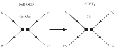
Figure 1: The figure shows the tree-level matching of $\mathrm{QED}$ onto $\mathrm{SCET_{I}}$, with EFT operators $Q_{9,\,10}$ and $\mathrm{SCET_{I}}$ operator $\mathcal{O}_{9}$ contributing, respectively. The notation and scaling of the $\mathrm{SCET_{I}}$ fields are given in Eq.(13). The heavy quark field $h_{v}$ in HQET is labelled by a double-solid line and (anti-)hard-collinear fields $\xi_{hc}$, $\tau_{hc}$ in $\mathrm{SCET_{I}}$ are denoted by double-dashed lines.

$$\mathcal{N}_{\Delta B=1}\,\sum_{k}\,C_{k}\,\left(\mu_{b}\right)Q_{k}\,=\,\sum_{i}\,\int du\,H_{i}\left(u,\mu_{b}\right)\,\mathcal{O}_{i}(u)\,,$$ (23)

where $i\,=\,9,\,E$. $C_{k}$ is the Wilson coefficient and $H_{i}$ represents hard function. By calculating the appropriate matrix elements in both sides of the equation above up to NLO in the order of $\alpha_{\mathrm{em}}$, firstly we get the hard functions at tree-level,

$$H_{9}^{(0)}\left(u,\mu_{b}\right) \,=\,\mathcal{N}\,\left[\,C_{9}^{(0)}\left(u,\mu_{b}\right)\,+\,C_{10}^{(0)}(\mu_{b})\,-\,\frac{2Q_{\ell}}{u}\,C_{7}^{(0)}\left(u,\mu_{b}\right)\,\right]\,,$$ (24)

$$H_{E}^{(0)}\left(u,\mu_{b}\right) \,=\,\mathcal{N}\,\left[\,-C_{10}^{(0)}(\mu_{b})\,\right]\,,$$ (25)

with

$$\mathcal{N}\,\equiv\,\mathcal{N}_{\Delta B=1}\,\frac{\alpha_{\mathrm{em}}\left(\mu_{b}\right)}{4\pi}\,,$$ (26)

where $C_{7\,,\,9\,,\,10}^{(0)}$ are the Wilson coefficients of $Q_{7\,,\,9\,,\,10}$ at LO in $\alpha_{\mathrm{em}}$. Formally, the contribution from four-quark operators $Q_{k}(k\,=\,1,\ldots,6)$ will start from one loop level. However these quark loops can be fully absorbed into effective Wilson coefficients $C_{7,\,9}^{\mathrm{eff}}$ Buras:1994dj , and then the hard function $H_{9}^{(0)}\left(u,\mu_{b}\right)$ decoupled from all four-quark operators $Q_{k}\,,k=1,\,...\,,6,\,7,\,9,\,10,$ at tree level should be replaced by

$$H_{9}^{(0)}\left(u,\mu_{b}\right)\,=\,\mathcal{N}\,\left[\,C_{9}^{\mathrm{eff}}\left(u,\mu_{b}\right)\,+\,C_{10}^{(0)}(\mu_{b})\,-\,\frac{2\,Q_{\ell}}{u}\,C_{7}^{\mathrm{eff}}\left(u,\mu_{b}\right)\,\right]\,.$$ (27)

For the case of an anti-hard-collinear quark, the hard function decoupled from $\mathcal{O}_{\bar{9}}$ is

$$H_{\bar{9}}^{(0)}\left(u,\mu_{b}\right) \,=\,\mathcal{N}\,\left[\,C_{9}^{\mathrm{eff}}\left(u,\mu_{b}\right)\,-\,C_{10}^{(0)}\left(\mu_{b}\right)\,-\,\frac{2Q_{\ell}}{u}\,C_{7}^{\mathrm{eff}}\left(u,\mu_{b}\right)\,\right]\,,$$ (28)

where the minus in front of $C_{10}^{(0)}\left(\mu_{b}\right)$ is due to the opposite relation of operator $\widetilde{\mathcal{O}}_{\overline{9}}\,$ and $\widetilde{\mathcal{O}}_{\overline{10}}\,$ in Eq.(18).

We can obtain the hard functions $H^{(1)}_{i}$ by expanding the matching equation at NLO as

$$\mathcal{N}_{\Delta B=1}\sum_{k}C^{(1)}_{k}\left(\mu_{b}\right)\langle Q_{k}\rangle^{(0)}=\sum_{i}\int du\left[H^{(0)}_{i}\left(u,\mu_{b}\right)\langle\mathcal{O}_{i}(u)\rangle^{(1)}+H^{(1)}_{i}\left(u,\mu_{b}\right)\langle\mathcal{O}_{i}(u)\rangle^{(0)}\right],$$

with

$$\langle\,\mathcal{O}_{i}(u)\,\rangle^{(1)}\,=\,Z_{ij}^{(1)}\,\langle\,\mathcal{O}_{j}(u)\,\rangle^{(0)}\,,$$ (30)

in Dimension Regulation, where $Z_{ij}^{(1)}$ is the UV renormalization factor of $\mathcal{O}_{j}(u)$. The Wilson coefficient $C^{(1)}_{k}$ represents the one at NLO of $\alpha_{\mathrm{em}}$. When we calculate the matrix element of l.h.s of Eq.(3.2.2) at NLO, more operators will be involved, which are written, without the position variables, as It is easy to find that $\mathcal{O}_{9,1}\,+\,\mathcal{O}_{9,2}\,=\,20\,\mathcal{O}_{9}$, $\mathcal{O}_{10,1}\,+\,\mathcal{O}_{10,2}\,=\,20\,\mathcal{O}_{10}$, and $\mathcal{O}_{9,1}\,=\,4\,\mathcal{O}_{9}$, $\mathcal{O}_{10,1}\,=\,4\,\mathcal{O}_{10}$ in $d=4$. We can possibly choose the following evanescent operators,

$$\begin{aligned} \mathcal{O}_{E_{1}}&\,\equiv\,{\mathcal{O}}_{9,1}\,-\,4\,{\mathcal{O}}_{9}\,,\\ \mathcal{O}_{E_{2}}&\,\equiv\,{\mathcal{O}}_{10,1}\,-\,4\,{\mathcal{O}}_{10}\\ &\,=\,{\mathcal{O}}_{10,1}\,-\,4\,\mathcal{O}_{9}\,+\,4\,\mathcal{O}_{E}\,.\end{aligned}$$ (31)

It is clearly that the physical operator ${\mathcal{O}}_{9}$ and the evanescent operators $\mathcal{O}_{E},\,\mathcal{O}_{E_{1}},\,\mathcal{O}_{E_{2}}$ will be contained in $\mathrm{SCET_{I}}$ when we consider the correction to NLO.

The hard functions at NLO can be extracted as

$$H^{(1)}_{i}\left(u,\mu_{b}\right)\,=\,\mathcal{N}\,C^{(1)}_{k}\left(\mu_{b}\right)\,-\,H^{(0)}_{j}\left(u,\mu_{b}\right)\,Z_{ji}^{(1)}\,,$$ (32)

with $k=7,\,9,\,10\,$ and $i\,\,\text{or}\,\,j=9\,,\,E\,,\,E_{1}\,,\,E_{2}$. In the following, we concentrate on $i=9$, and the hard function associate with physical operator ${\mathcal{O}}_{9}$ is

$$H^{(1)}_{9}\left(u,\mu_{b}\right)=\mathcal{N}\left[\,C^{(1)}_{7,\,9}\left(\mu_{b}\right)+C^{(1)}_{10}\left(\mu_{b}\right)\,\right]-H^{(0)}_{9}\left(u,\mu_{b}\right)\,Z_{99}^{(1)}-H^{(0)}_{E}\left(u,\mu_{b}\right)\,Z_{E9}^{(1)}\,,$$ (33)

where terms for $j=E_{1}\,,\,E_{2}$ disappear due to $H^{(0)}_{E_{1},\,E_{2}}=0$. Next it is necessary to calculate the matrix element of evanescent operator $\mathcal{O}_{E}$ at NLO to check whether $\mathcal{O}_{E}$ would contribute to hard function $H^{(1)}_{9}$ or not, and the result is

$$\langle\mathcal{O}_{E}\,\rangle^{(1)}\,\sim\,H_{E}^{(1)}\,\langle\mathcal{O}_{E}\,\rangle^{(0)}\,,$$ (34)

where the physical amplitude $\langle{\mathcal{O}}_{9}\,\rangle^{(0)}\,$ do not appear. It means that evanescent operator $\mathcal{O}_{E}$ does not have an influence on hard function $H_{9}$ at one loop level and Eq.(33) can be reduced to

$$H^{(1)}_{9}\left(u,\mu_{b}\right)\,=\,\mathcal{N}\,\left[\,C^{(1)}_{7,\,9}\left(\mu_{b}\right)\,+\,C^{(1)}_{10}\left(\mu_{b}\right)\,\right]\,-\,H^{(0)}_{9}\left(u,\mu_{b}\right)\,Z_{99}^{(1)}\,.$$ (35)

For the case of an anti-hard-collinear quark $\mathcal{O}_{\bar{9}}$, the corresponding hard function is

$$H_{\bar{9}}^{(1)}\left(u,\mu_{b}\right)\,=\,\mathcal{N}\,\left[C^{(1)}_{\bar{7},\,\bar{9}}\left(\mu_{b}\right)\,-\,C^{(1)}_{\overline{10}}\left(\mu_{b}\right)\right]\,-\,H^{(0)}_{\bar{9}}\left(u,\mu_{b}\right)\,Z_{\bar{9}\bar{9}}^{(1)}\,,$$ (36)

where the second terms in r.h.s of both Eqs.(35) and (36) are the IR subtractions to cancel the IR divergences from their first terms.

The first terms in Eqs.(35) and (36) are from one loop contributions with $Q_{k}$ and $Q_{\bar{k}}$,  $k=7,\,9,\,10,$ inserted in Fig.(2), which are corresponding to the diagrams with a hard-collinear and an anti-hard-collinear light quark state, respectively.

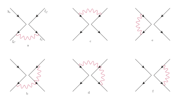
Figure 2: one-loop QED corrections to hard functions

We find that the results in the case of the hard-collinear sector are only equal to ones of the anti-hard-collinear sector for Figs.(e) and (f), while opposite for Figs.(a)-(d), e.g.

$$\begin{aligned} C_{k}^{\text{(a)}}\,&=\,-\,C_{\bar{k}}^{\text{(b)}}\,,\quad\quad C_{k}^{\text{(b)}}\,=\,-\,C_{\bar{k}}^{\text{(a)}}\,,\\ C_{k}^{\text{(c)}}\,&=\,-\,C_{\bar{k}}^{\text{(d)}}\,,\quad\quad C_{k}^{\text{(d)}}\,=\,-\,C_{\bar{k}}^{\text{(c)}}\,,\\ C_{k}^{\text{(e)}}\,&=\,\,C_{\bar{k}}^{\text{(e)}}\,,\quad\quad\quad C_{k}^{\text{(f)}}\,=\,\,C_{\bar{k}}^{\text{(f)}}\,,\end{aligned}$$ (37)

where $C_{k}^{\text{(a-f)}}$ denotes contribution from hard mode integrated out from each diagram in Fig.(2). It is clearly that the case in Eq.(37) is different from the one at tree level, $C_{k}^{(0)}\,=\,C_{\overline{k}}^{(0)}$. Parts of these QED corrections ($C_{k}^{\text{(a-d)}}$) are antisymmetric under the exchange of the collinear and anti-collinear sectors once hard fluctuations are decoupled. The reason is that the exchange of the collinear and anti-collinear light quark is equivalent to performing the charge conjugation (C) just for final leptons as shown in the r.h.s of Fig.(2), that is, the matrix element, with one photon attached to one of leptons, will be transformed with C operator and simultaneously be matched onto $\mathrm{SCET_{I}}$ as

$$\left\langle\gamma\,\left|Q_{i},\mathcal{L}_{\mathrm{QED}}\,\right|\,\ell^{+}\,\ell^{-}\,\right\rangle\,\stackrel{{\scriptstyle\mathrm{C}}}{{\longrightarrow}}\,-\,\left\langle 0\,\left|\,\mathcal{O}_{\bar{i}}\,\right|\,\ell^{+}\,\ell^{-}\,\right\rangle\,,$$ (38)

where operator $Q_{i}$ is changed into $Q_{\bar{i}}$ after C operator transition. Lagrangian $\mathcal{L}_{\mathrm{QED}}$ is C operator invariant, and the minus in r.h.s of above formula is from the action of C operator on one photon attached to the one of leptonic fields. It is possible to write Eq.(38) into a more general form to arbitrary loop order,

$$\left\langle\,m\,\gamma\,\left|\,Q_{i},\mathcal{L}_{\mathrm{QED}}\,\right|\,\ell^{+}\,\ell^{-}\,\right\rangle\,\stackrel{{\scriptstyle\mathrm{C}}}{{\longrightarrow}}\,(-1)^{m}\,\left\langle\,0\,\left|\,\mathcal{O}_{\bar{i}}\,\right|\,\ell^{+}\,\ell^{-}\,\right\rangle\,,$$ (39)

where $m$ stands for the number of photon attached to lepton sector and determines whether the hard functions are symmetric or antisymmetric under the exchange of the collinear and anti-collinear light quark fields, that is, the relations, $C_{k}^{(m)}=(-1)^{m}\,C_{\bar{k}}^{(m)},\,m=0,\,1,\,2,\,...\,,$ are valid to all orders in $\alpha_{\mathrm{em}}$.

Based on these relations between $C_{k}^{(a-f)}$ and $C_{\bar{k}}^{(a-f)}$ in Eq.(37) and the one between $\mathcal{O}_{9}$ and $\mathcal{O}_{10}$ in Eq.(18), the hard functions for $i=9$ at NLO in Eqs.(35) and (36) can be simplified considerably as

$$\begin{aligned} H^{(1)}_{9}\left(u,\mu_{b}\right)+H^{(1)}_{\bar{9}}\left(u,\mu_{b}\right)&=2\mathcal{N}\left[\,C_{7,\,9}^{(e-f)}\left(\mu_{b}\right)+C_{10}^{(a-d)}\left(\mu_{b}\right)\,\right]-\text{IR subtractions}\,\end{aligned}$$ (40)

which implied that $H^{(1)}_{9}$ equals to $H^{(1)}_{\bar{9}}$ and the hard function can be written as

$$H^{(1)}_{9/\bar{9}}\left(u,\mu_{b}\right)\, =\,\mathcal{N}\,\left[\,C_{7,\,9}^{(e-f)}\left(\mu_{b}\right)\,+\,C_{10}^{(a-d)}\left(\mu_{b}\right)\,\right]\,-\,\text{IR subtractions}\,,$$ (41)

with the result as follows,

$$\begin{aligned} H^{(1)}_{9/\bar{9}}&\,=\,(C_{9}^{\mathrm{eff}}-\frac{2Q_{\ell}}{u}C_{7}^{\mathrm{eff}})\left(\frac{\alpha_{\mathrm{em}}}{4\pi}Q_{b}Q_{q}+\frac{\alpha_{\mathrm{s}}}{4\pi}C_{F}\right)\left[-\ln^{2}\frac{\tilde{r}}{\bar{u}}-2\ln\frac{\tilde{r}}{\bar{u}}+\frac{1}{2}\ln^{2}\tilde{r}+2\mathrm{Li}_{2}(-\frac{u}{\bar{u}})-4-\frac{\pi^{2}}{12}\right]\\ &+(C_{9}^{\mathrm{eff}}-\frac{2Q_{\ell}}{u}C_{7}^{\mathrm{eff}})\frac{\alpha_{\mathrm{em}}}{4\pi}Q_{\ell}^{2}\,\left[-\ln^{2}\frac{-u-i0}{\tilde{r}}+3\ln\frac{-u-i0}{\tilde{r}}-8+\frac{\pi^{2}}{6}\right]\\ &+C_{9}^{\mathrm{eff}}\left(\frac{\alpha_{\mathrm{em}}}{4\pi}Q_{b}Q_{q}+\frac{\alpha_{\mathrm{s}}}{4\pi}C_{F}\right)\left[\ln\tilde{r}-\frac{\bar{u}}{u}\ln\bar{u}\right]\\ &+C_{10}\frac{\alpha_{\mathrm{em}}}{4\pi}Q_{\ell}Q_{q}\left[-\ln^{2}\frac{u}{r}-\ln^{2}\frac{-\bar{u}-i0}{r}+\frac{2\ln u}{\bar{u}}+\ln^{2}r+3\ln r+2\operatorname{Li}_{2}\left(-\frac{\bar{u}}{u}\right)+10+\frac{\pi^{2}}{6}\right]\,,\end{aligned}$$ (42)

where $Q_{\ell}\,=\,-1,\,Q_{q}\,=-\,1/3$, $\tilde{r}\,=\,(\mu^{2}/m_{b}^{2})\,\mathrm{e}^{\gamma_{E}}$. The hard function $H^{(1)}_{9/\bar{9}}$ has also contained QCD corrections which can be obtained with the replacement of $(\alpha_{\mathrm{em}}/4\pi)\,Q_{b}\,Q_{q}\,$ in QED contributions in above formula by $(\alpha_{\mathrm{s}}/4\pi)\,C_{F}$.

3.3 $\mathrm{HQET}\times\mathrm{bHLET}$

The first step of matching from $\mathrm{QCD}\times\mathrm{QED}$ onto $\mathrm{SCET_{I}}$ for $B_{q}\,\to\,\tau^{+}\,\tau^{-}$ described above is same as for $B_{q}\,\to\,\mu^{+}\,\mu^{-}$. However, as for massive $\tau$ final states, $m_{\tau}^{2}\,\sim\,m_{b}\,\Lambda_{\mathrm{QCD}}$, the next matching from $\mathrm{SCET_{I}}$ will be different from the case in $\mu$ leptonic decays where the (anti-)hard-collinear leptons need to turn into (anti-)collinear ones by matching onto $\mathrm{SCET_{II}}$. The leptonic fields in $B_{q}\,\to\,\tau^{+}\,\tau^{-}$ decay should be converted to a soft-collinear field after integrating out the hard-collinear massive $\tau$ scale as done for massive $b$ quark fiels in the process $W\to B\gamma$ Beneke:2023nmj in bHQET. Consequently, in the following, we need to perform matching from $\mathrm{SCET_{I}}$ to $\mathrm{HQET}$ to turn the hard-collinear light antiquark to a soft one to get a non-vanishing overlap $B$-meson state and simultaneously match onto $\mathrm{bHLET}$ to make the hard-collinear $\tau$ lepton to be a soft-collinear one.

3.3.1 Operators

The hard-collinear antiquark field of $\mathcal{O}_{9}$ in $\mathrm{SCET_{I}}$ can turn into a soft antiquark field through emission of a hard-collinear photon by the power-suppressed $\mathrm{SCET_{I}}$ Lagrangian,

$$\mathcal{L}_{\xi q}^{(1)}\,=\,\bar{q}_{s}\left(x_{-}\right)\,\left[W_{\xi,\,hc}\,W_{hc}\right]^{\dagger}(x)\,i\,\not{D}_{hc\perp}\,\xi_{hc}(x)\,+\,\mathrm{h.c.}\,$$ (43)

and analogously for anti-hard-collinear fields with the replacements of $hc\,\rightarrow\,\overline{hc},\,n_{+}\,\rightarrow\,n_{-}$ and $x_{-}\,\rightarrow\,x_{+}$. $W_{\xi,\,hc}\,\text{and}\,W_{hc}$, connected with $\xi_{hc}(x)$, are Wilson lines of hard-collinear photons and gluons,

$$W_{\xi,hc}(x) \,\equiv\,\exp\,\left[\,i\,e\,Q_{\xi}\,\int_{-\infty}^{0}\,ds\,n_{+}A_{hc}\left(x+sn_{+}\right)\,\right],$$ (44)

$$W_{hc}(x) \,\equiv\,\mathcal{P}\,\exp\,\left[\,i\,g_{s}\,\int_{-\infty}^{0}\,ds\,n_{+}G_{hc}\left(x+sn_{+}\right)\,\right],$$ (45)

respectively. Then the hard-collinear photon field, $A_{hc\perp}$ from $D_{hc\perp}$ in Eq.(43), would be followed by the fusion,

$$\bar{\ell}_{hc}\,+\,A_{\perp hc}\,\stackrel{{\scriptstyle}}{{\rightarrow}}\,m_{\tau}\,\bar{\ell}_{hc}\,,$$ (46)

through the leading power Lagrangian relevant to mass term,

$$\mathcal{L}_{m}^{(0)}(y) \,=\,m_{\tau}\,\bar{\ell}_{C}\,\left[\,i\,\not{D}_{C\perp}\,,\,\frac{1}{i\,n_{+}\,D_{C}}\,\right]\,\frac{\not{n}_{+}}{2}\,\ell_{C}\,.$$ (47)

Therefore, we will match the time-ordered product of the $\mathrm{SCET_{I}}$ operators $\mathcal{O}_{9}(u)$ with $\mathcal{L}_{\xi q}^{(1)}(x)$ and $\mathcal{L}_{m}^{(0)}(y)$,

$$\left\langle\,\ell^{-}(p_{\ell})\,\ell^{+}\left(p_{\bar{\ell}}\right)\,\left|\,\int d^{4}x\,\int d^{4}y\,T\,\left\{\mathcal{O}_{9}(u),\,\mathcal{L}_{\xi q}^{(1)}(x),\,\mathcal{L}_{m}^{(0)}(y)\right\}\,\right|\,b\left(p_{b}\right)\,q\left(\ell_{q}\right)\,\right\rangle\,,$$ (48)

to the corresponding matrix element of operator in $\mathrm{HQET}\times\mathrm{bHLET}$.

The systematic constructions of $\mathrm{HQET}\times\mathrm{bHLET}$ operators according to the analysis on a power-counting in $\lambda$, canonical dimension $d$, reparametrization symmetry of SCET, gauge symmetry and helicity conservation and so on, are similar to the ones performed in heavy-to-light meson form factors Beneke:2003pa and the case of $B_{q}\,\to\,\mu^{+}\,\mu^{-}$ in Appendix B of Beneke:2019slt . At leading power, the $\mathrm{HQET}\times\mathrm{bHLET}$ operators used for the matching onto time-ordered product in Eq.(48) can be defined in position space as

$$\widetilde{\mathcal{J}}_{m\chi}^{A1}(v) \,=\,\bar{q}_{s}\left(vn_{-}\right)Y\left(vn_{-},0\right)\frac{\not{n}_{-}}{2}P_{L}h_{v}(0)[Y_{+}^{\dagger}Y_{-}](0)\left[\bar{\ell}_{sc}(0)\,\left(4P_{R}\right)\ell_{\overline{sc}}(0)\right]\,,$$ (49)

and

$$\widetilde{\mathcal{J}}_{m\bar{\chi}}^{A1}(v) =\bar{q}_{s}\left(vn_{+}\right)Y\left(vn_{+},0\right)\frac{\not{n}_{+}}{2}P_{L}h_{v}(0)[Y_{+}^{\dagger}Y_{-}](0)\left[\bar{\ell}_{sc}(0)\left(4P_{R}\right)\ell_{\overline{sc}}(0)\right]\,,$$ (50)

for analogous operators generated from the matching relevant with $\mathcal{O}_{\bar{9}}$, where the soft light antiquark field $\bar{q}_{s}\left(vn_{-}\right)$ has been delocalized along the $n_{-}$ direction of light-cone through integrating out small component $n_{-}\ell_{q}$ of hard-collinear light quark. The roles of $n_{-}$ and $n_{+}$ are reversed for $\bar{q}_{s}\left(vn_{+}\right)$ when the anti-hard-collinear mode is integrated out. $Y\left(vn_{+},0\right)$ is the finite-distance Wilson line defined as

$$Y(x,y)\,=\,\exp\,\left[\,i\,e\,Q_{q}\,\int_{y}^{x}\,dz_{\mu}\,A_{s}^{\mu}(z)\,\right]\,\mathcal{P}\,\exp\,\left[\,i\,g_{s}\,\int_{y}^{x}\,dz_{\mu}\,G_{s}^{\mu}(z)\,\right]\,,$$ (51)

to connect non-local field $\bar{q}_{s}\left(vn_{+}\right)$ to $h_{v}(0)$ to maintain QCD and QED gauge invariance of non-local operator. Here $\mathcal{P}$ is the path-ordering operator. $A_{s}^{\mu}(z)$ and $G_{s}^{\mu}\,=\,G_{s}^{\mu A}\,T^{A}$ are the soft photon and gluon fields, respectively. The product of Wilson lines $\left[\,Y_{+}^{\dagger}Y_{-}\,\right](0)\,\equiv\,Y_{+}^{\dagger}(0)\,Y_{-}(0)$ appears after decoupling of soft photons from the hard-collinear and anti-hard-collinear leptons in $\mathrm{SCET}_{\mathrm{I}}$, respectively, with their small component $n_{-}p_{\ell}$ and $n_{+}p_{\bar{\ell}}$ scaling as $\lambda^{2}$ in the same order as soft photons. The soft electromagnetic Wilson lines are defined as

$$Y_{\pm}(x)\,=\,\exp\,\left[\,-i\,e\,Q_{\ell}\,\int_{0}^{\infty}\,ds\,n_{\mp}A_{s}\left(x+sn_{\mp}\right)\,\right]\,.$$ (52)

For $\tau$ final states here, there is no so-called $B1$-type operator as appeared in the case of $\mu$ leptons attributing to collinear contribution. It is only one way as Eq.(46) to built $A1$-type operator in $\mathrm{HQET}\times\mathrm{bHLET}$.

We define the Fourier transforms of $\widetilde{\mathcal{J}}_{i}^{A1}(v)$ in order to do matching from $\mathrm{SCET_{I}}$ to $\mathrm{HQET}\times\mathrm{bHLET}$ in momentum space as

$$\mathcal{J}_{i}^{A1}(\omega)\,=\,\int\,\frac{dv}{2\pi}\,e^{i\,\omega\,v}\,\widetilde{\mathcal{J}}_{i}^{A1}(v)\,,$$ (53)

where $\omega$ corresponds to the soft momentum of the light quark along the $n_{+}$ and $n_{-}$ direction for $i=m\chi\,\text{and}\,m\bar{\chi}$, respectively.

3.3.2 Matching from $\mathrm{SCET_{I}}$ to $\text{HQET}\times\text{bHLET}$

We perform the matching of operator $\mathcal{O}_{9}$ in $\mathrm{SCET_{I}}$ onto $\mathcal{J}_{m\chi}^{A1}$ in $\mathrm{HQET}\times\mathrm{bHLET}$ at hard-collinear scale $\mu_{hc}$,

$$\mathcal{O}_{9}(u) \,\rightarrow\,\int\,d\omega\,J_{m}(u;\omega)\,\mathcal{J}_{m\chi}^{A1}(\omega)\,.$$ (54)

As mentioned in Sec.3.3.1, the operator in l.h.s of Eq.(54) should be connected with two currents $\mathcal{L}_{\xi q}^{(1)}(x)\,\text{and}\,\mathcal{L}_{m}^{(0)}(y)$ to produce a non-vanishing overlap $B$-meson state and bHLET modes. The tree-level matching relation is depicted in Fig.(3).

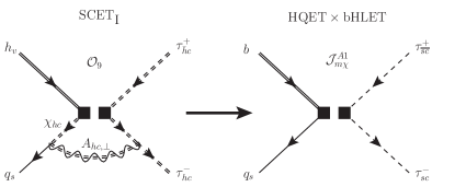
Figure 3: The figure shows the tree-level matching of $\mathrm{SCET_{I}}$ onto $\mathrm{HQET}\times\mathrm{bHLET}$, where $\mathrm{SCET_{I}}$ operator $\mathcal{O}_{9}$ connected with two currents forms a time-ordered product to match onto $A1$-type operator $\mathcal{J}_{m\chi}^{A1}$. The double-dashed lines accompanied by a wavy line depict the hard-collinear photon field $A_{hc,\,\perp}$ in $\mathrm{SCET_{I}}$. The single-solid line and single-dotted line in $\mathcal{J}_{m\chi}^{A1}$ represent the soft spectator quark field $q_{s}$ and soft-collinear $\tau$ fields.

Firstly, we need to calculate the matrix element of the time-ordered product of the $\mathrm{SCET_{I}}$ operators $\mathcal{O}_{9}(u)$ with $\mathcal{L}_{\xi q}^{(1)}(x)$ and $\mathcal{L}_{m}^{(0)}(y)$,

$$\langle\,\ell^{-}(p_{\ell^{-}})\,\ell^{+}\left(p_{\ell^{+}}\right)\,|\,\int d^{4}x\,\int d^{4}y\,T\,\{\mathcal{O}_{9}(u),\,\mathcal{L}_{\xi q}^{(1)}(x),\,\mathcal{L}_{m}^{(0)}(y)\}\,|b\left(p_{b}\right)\,q\left(\ell_{q}\right)\,\rangle\,,$$ (55)

and the result is

$$\frac{\alpha_{\mathrm{em}}}{4\pi}\,Q_{\ell}\,Q_{s}\,m_{\ell}\,\frac{\bar{u}}{\omega}\,\ln\,[\,1\,+\,\frac{u}{\bar{u}}\,\frac{\omega\,n_{+}p_{\ell^{-}}}{m_{\ell}^{2}}\,]\,\theta(u)\,\theta(\bar{u})\,\,[\,\bar{q}_{s}\,\gamma^{\perp}_{\nu}\,\gamma^{\perp}_{\mu}\,\frac{\not{n}_{-}}{2}\,P_{L}\,h_{v}\,]\,[\,\bar{\ell}_{sc}\,\,\gamma_{\perp}^{\nu}\,\gamma_{\perp}^{\mu}\,\ell_{\overline{sc}}\,]\,.$$ (56)

We can define a matrix element of an operator denoted by $\mathcal{J}_{9}^{A1}$ as

$$\langle\mathcal{J}_{9}^{A1}\rangle\,\equiv\,\left[\,\bar{q}_{s}(l_{q})\,\gamma^{\perp}_{\nu}\,\gamma^{\perp}_{\mu}\,(\not{n}_{-}/2)\,P_{L}\,h_{v}(p_{b})\,\right]\,\left[\,\bar{\ell}_{sc}(p_{\ell^{-}})\,\gamma_{\perp}^{\nu}\,\gamma_{\perp}^{\mu}\,\ell_{\overline{sc}}(p_{\ell^{+}})\,\right]\,.$$ (57)

$\mathcal{J}_{9}^{A1}$ is equal to $\mathcal{J}_{m\chi}^{A1}$ in dimension $d=4$,

$$\mathcal{J}_{9}^{A1}\,\stackrel{{\scriptstyle\mathrm{d=4}}}{{\longrightarrow}}\,\mathcal{J}_{m\chi}^{A1}\,,$$ (58)

so that we can define an evanescent operator as

$$\mathcal{J}_{E}^{A1}\,=\,\mathcal{J}_{9}^{A1}\,-\,\mathcal{J}_{m\chi}^{A1}\,.$$ (59)

Hard-collinear function $J_{m}(u,\omega)$ can be extracted from the matching equation at tree level,

$$C_{9m}^{(0)}\,\langle\mathcal{J}_{9}^{A1}(u)\rangle^{(0)}\,=\,\int\,d\omega\,\left[\,J_{m}^{(0)}(u;\omega)\,\langle\mathcal{J}_{m\chi}^{A1}(\omega)\rangle^{(0)}\,+\,J_{E}^{(0)}(u;\omega)\,\langle\mathcal{J}_{E}^{A1}(u)\rangle^{(0)}\,\right]\,,$$ (60)

where the coefficient $C_{9m}^{(0)}\,$ can be read from the result of Eq.(56),

$$C_{9m}^{(0)}\,=\,\frac{\alpha_{\mathrm{em}}}{4\pi}\,Q_{\ell}\,Q_{s}\,m_{\ell}\,\frac{\bar{u}}{\omega}\,\ln\,\left(\,1\,+\,\frac{u}{\bar{u}}\,\frac{\omega\,n_{+}p_{\ell^{-}}}{m_{\ell}^{2}}\,\right)\,\theta(u)\,\theta(\bar{u})\,.$$ (61)

At tree level, the hard-collinear function $J_{m}(u,\omega)$ is just $C_{9m}^{(0)}$,

$$J_{m}^{(0)}(u;\omega;\mu=\mu_{hc}) \,=\,\frac{\alpha_{\mathrm{em}}}{4\pi}\,Q_{\ell}\,Q_{s}\,m_{\ell}\,\frac{\bar{u}}{\omega}\,\ln\,\left(\,1\,+\,\frac{u}{\bar{u}}\,\frac{\omega\,n_{+}p_{\ell^{-}}}{m_{\ell}^{2}}\,\right)\,\theta(u)\,\theta(\bar{u})\,,$$ (62)

at hard-collinear scale $\mu_{hc}$, and the result for $J_{\overline{m}}^{(0)}$ can be obtained by the replacement of $n_{+}p_{\ell^{-}}\,\rightarrow\,n_{-}p_{\ell^{+}}$.

3.4 Matrix elements of operators $\widetilde{\mathcal{J}}_{m\chi,\bar{\chi}}^{A1}$ in $\mathrm{HQET}\times\mathrm{bHLET}$

The operators $\widetilde{\mathcal{J}}_{m\chi,\bar{\chi}}^{A1}$ in Eqs.(49) and (50) are composed of soft, soft-collinear sector and anti-soft-collinear sector, and these fields do not interact with one another, which implies that the matrix elements of the operators $\widetilde{\mathcal{J}}_{m\chi,\bar{\chi}}^{A1}$ can be further factorized accordingly into matrix elements of the separate factors in the respective soft, soft-collinear and anti-soft-collinear Hilbert space,

$$\langle\,\ell^{+}\,\ell^{-}\,|\,\widetilde{\mathcal{J}}_{m\chi}^{A1}\,|\,\bar{B}_{q}\,\rangle\,=\,\langle\,0\,|\,\widehat{\mathcal{J}}_{s}\,|\,\bar{B}_{q}\,\rangle\,\langle\,\ell^{-}\,|\,\widehat{\mathcal{J}}_{sc}\,|\,0\,\rangle\,\langle\,\ell^{+}\,|\,\widehat{\mathcal{J}}_{\overline{sc}}\,|\,0\,\rangle\,.$$ (63)

Then the soft, (anti-)soft-collinear sectors are defined as

$$\widehat{\mathcal{J}}_{s} \,=\,\bar{q}_{s}\left(vn_{-}\right)\,Y\left(vn_{-},0\right)\,\frac{\not\!n_{-}}{2}\,P_{L}\,h_{v}(0)\,[Y_{+}^{\dagger}\,Y_{-}](0)\,,$$ (64)

$$\widehat{\mathcal{J}}_{sc} \,=\,\bar{\ell}_{sc}(0)\,\left(4P_{R}\right)\,,\,\quad\widehat{\mathcal{J}}_{\overline{sc}}\,=\,\ell_{\overline{sc}}(0)\,.$$ (65)

However, when considering the renormalization of each sector separately, one find IR-divergence can not be cancelled only in soft sector, and the remaining divergence need to be cancelled by the one from (anti-)soft-collinear sectors (more details can be found in Section 4.2 of Ref. Beneke:2019slt ). This appears to be in conflict with the factorization of the soft and (anti-)soft-collinear sectors. It is so-called factorization anomaly, which will lead to a rearrangement for soft operator. In order to subtract the remaining IR-divergence in soft operator, one can redefine and renormalize soft function as

$$\widetilde{\mathcal{J}}_{s}(v)\,\equiv\,\frac{\widehat{\mathcal{J}}_{s}(v)}{\,\langle\,0\,|\,[\,Y_{+}^{\dagger}\,Y_{-}\,](0)\,|\,0\,\rangle}\,,$$ (66)

where $\langle\,0\,|\,[\,Y_{+}^{\dagger}\,Y_{-}\,]\,(0)\,|\,0\,\rangle$ in the denominator is just the overlap term between soft and (anti-)soft-collinear regions. It can be divided into two separate factors $R_{+}$ and $R_{-}$ by $\,\langle\,0\,|\,[\,Y_{+}^{\dagger}\,Y_{-}\,]\,(0)\,|\,0\,\rangle\,\equiv\,R_{+}\,R_{-}$, where $R_{+}$ and $R_{-}$ can be chosen as a symmetric form upon exchanging $n_{+}\leftrightarrow n_{-}$. Then soft-collinear sector and anti-soft-collinear sector are redefined correspondingly as

$$\widetilde{\mathcal{J}}_{sc} \,=\,R_{+}\,\overline{\ell}_{sc}(0)\,\left(\,4\,P_{R}\,\right)\,,\,\quad\widetilde{\mathcal{J}}_{\overline{sc}}\,=\,R_{-}\,\ell_{\overline{sc}}(0)\,.$$ (67)

The hadronic matrix element of the soft operator $\,\langle\,0\,|\,\widetilde{\mathcal{J}}_{s}\,|\,B_{q}\,\rangle$ is related to the $B_{q}$ meson decay constant and the leading-twist $B_{q}$ meson LCDA Grozin:1996pq ; Beneke:2000wa . However, it would not coincide with the universal $B_{q}$ meson LCDA but depend on the final-state particles of the specific process due to appearance of additional soft QED Wilson lines $Y_{+}^{\dagger}\,Y_{-}$. Therefore, we define the $\langle\,0\,|\,\widetilde{\mathcal{J}}_{s}\,|\,B_{q}\,\rangle$ as a generalized and process-dependent $B_{q}$ meson LCDA $\Phi_{+}(\omega)$,

$$\begin{aligned} (-4)\,\langle\,0\,|\,\widetilde{\mathcal{J}}_{s}(v)\,|\,\bar{B}_{q}(p)\,\rangle&\,=\,\frac{\,\langle\,0\,|\,\bar{q}_{s}\left(vn_{-}\right)\,Y\left(vn_{-},0\right)\,\not\!n_{-}\,\gamma_{5}\,h_{v}(0)\,Y_{+}^{\dagger}(0)\,Y_{-}(0)\,|\,\bar{B}_{q}(p)\,\rangle}{\,\langle\,0\,|\,[\,Y_{+}^{\dagger}\,Y_{-}\,]\,(0)\,|\,0\,\rangle}\\ &\,\equiv\,i\,m_{B_{q}}\,\int_{0}^{\infty}\,d\omega\,e^{-i\,\omega\,v}\,\mathcal{F}_{B_{q}}\,\Phi_{+}(\omega)\,.\end{aligned}$$ (68)

The analogous definition holds for the anti-collinear case by interchanging $n_{+}\,\leftrightarrow\,n_{-}$ but with the same $B_{q}$ meson LCDA $\Phi_{+}(\omega)$. $\mathcal{F}_{B_{q}}$ is the generalized process-dependent $B_{q}$ meson decay constant, which can be defined through the local matrix element,

$$\frac{\,\langle\,0\,|\,\bar{q}_{s}(0)\,\gamma^{\mu}\,\gamma_{5}\,h_{v}(0)\,Y_{+}^{\dagger}(0)\,Y_{-}(0)\,|\,\bar{B}_{q}(p)\,\rangle}{\,\langle\,0\,|\,[\,Y_{+}^{\dagger}\,Y_{-}]\,(0)\,|\,0\,\rangle}\,\equiv\,i\,\mathcal{F}_{B_{q}}\,m_{B_{q}}\,v^{\mu}\,.$$ (69)

Although the specific process-dependent $B_{q}$ meson LCDA and decay constant in Eqs.(68) and (69) are complicated in the presence of QED effects, we can expand them perturbatively in terms of $\alpha_{\mathrm{em}}$ at the soft scale $\mu_{s}\,\sim\,\Lambda_{\mathrm{QCD}}$,

$$\mathcal{F}_{B_{q}}\left(\mu_{s}\right) \,=\,\sum_{n=0}^{\infty}\,\left(\,\frac{\alpha_{\mathrm{em}}\left(\mu_{s}\right)}{4\,\pi}\right)^{n}\,F_{B_{q}}^{(n)}\left(\mu_{s}\right)\,,$$ (70)

$$\mathcal{F}_{B_{q}}\left(\mu_{s}\right)\,\Phi_{+}\left(\omega;\mu_{s}\right) \,=\,\sum_{n=0}^{\infty}\,\,\sum_{k=0}^{\infty}\,\left(\,\frac{\alpha_{\mathrm{em}}\left(\mu_{s}\right)}{4\,\pi}\right)^{n+k}\,F_{B_{q}}^{(n)}\left(\mu_{s}\right)\,\phi_{+}^{(k)}\left(\omega;\mu_{s}\right)\,,$$ (71)

where the leading terms, $n=0$ and $k=0$, are just the standard $B_{q}$ meson decay constant $F_{B_{q}}(\mu_{s})$ and $\operatorname{LCDA},\phi_{+}(\omega;\mu_{s})$, defined in the absence of QED correction. Higher-order terms starting from $n=1$ or $k=1$ in the expansion with QCD and QED correction simultaneously are non-universal, non-local HQET matrix elements that have to be evaluated nonperturbatively. Fortunately, only the universal objects $F_{B_{q}}(\mu_{s})$ and $\phi_{+}(\omega;\mu_{s})$ need to be known at the leading and next-to-leading logarithmic (NLL) accuracy.

Next the matrix element of (anti-)soft-collinear in Eq.(67) can be defined after renormalization by

$$\left\langle\ell^{-}\left(p_{\ell^{-}}\right)\left|R_{+}\bar{\ell}_{sc}(0)\right|0\right\rangle=Z_{\ell}\bar{u}_{sc}\left(p_{\ell^{-}}\right),\quad\left\langle\ell^{+}\left(p_{\ell^{+}}\right)\left|R_{-}\ell_{\overline{sc}}(0)\right|0\right\rangle=Z_{\bar{\ell}}v_{\overline{sc}}\left(p_{\ell^{+}}\right)\,,$$ (72)

where

$$Z_{\ell}\,=\,Z_{\bar{\ell}}\,=\,1\,+\,\mathcal{O}\left(\alpha_{\mathrm{em}}\right)\,.$$ (73)

Collecting the soft and (anti-)soft-collinear sectors in Eqs.(68) and (72), respectively, we can now derive the factorized expression for the matrix element of Eq.(63) in the Fourier transformed form,

$$\left\langle\,\ell^{+}\left(p_{\ell^{+}}\right)\,\ell^{-}\left(p_{\ell^{-}}\right)\,\left|\,\mathcal{J}_{m\chi}^{A1}(\omega)\,\right|\,\bar{B}_{q}(p)\,\right\rangle\,=\,T_{+}\,m_{B_{q}}\,\mathcal{F}_{B_{q}}\,\Phi_{+}(\omega)\,,$$ (74)

where

$$T_{+}(\mu)\,\equiv\,(-i)\,m_{\ell}(\mu)\,Z_{\ell}(\mu)\,Z_{\bar{\ell}}(\mu)\,\left[\,\bar{u}_{sc}\left(p_{\ell^{-}}\right)\,P_{R}\,v_{\overline{sc}}\left(p_{\ell^{+}}\right)\,\right]\,.$$ (75)

The same result holds for the anti-soft-collinear operators $\mathcal{J}_{m\bar{\chi}}^{A1}$ owning to the same soft matrix element definition in Eq.(68).

4 Resummed amplitude of $B_{q}\,\rightarrow\,\tau^{+}\,\tau^{-}$

4.1 Factorization of the amplitude

After factorizing $B_{q}\,\rightarrow\,\tau^{+}\,\tau^{-}$ decay into three parts: hard function, (anti-)hard-collinear function and soft function, in Sec.3, we can thus write the complete expression of its amplitude by adding the hard function and hard-collinear matching coefficients to Eq.(74) as

$$i\,\mathcal{A}_{9} =T_{+}\int_{0}^{1}du\left[H_{9}^{(0)}(u,\mu)+H_{\bar{9}}^{(0)}(u,\mu)+2H^{(1)}_{9/\bar{9}}(u,\mu)\right]\int_{0}^{\infty}d\omega J_{m}(u;\omega,\mu)m_{B_{q}}\mathcal{F}_{B_{q}}(\mu)\Phi_{+}(\omega,\mu),$$

$$=\,T_{+}\,\int_{0}^{1}du\,2H_{9}(u,\mu)\,\int_{0}^{\infty}\,d\omega\,J_{m}(u;\omega,\mu)\,m_{B_{q}}\,\mathcal{F}_{B_{q}}(\mu)\,\Phi_{+}(\omega,\mu)\,,$$ (76)

where $H^{(0)}_{9},\,H^{(0)}_{\bar{9}},\,H^{(1)}_{9/\bar{9}}$ are shown in Eqs.(27), (28) and (42), respectively. The summation of them can be simplified as

$$2\,H_{9}\left(u,\mu_{b}\right)\, =2\mathcal{N}\,\left[\,C_{9}^{\mathrm{eff}}\left(u,\mu_{b}\right)\,-\,\frac{2\,Q_{\ell}}{u}\,C_{7}^{\mathrm{eff}}\left(u,\mu_{b}\right)\,\right]\,+\,2H^{(1)}_{9/\bar{9}}\,,$$ (77)

where the contribution $C^{(0)}_{10}$ from operator $Q_{10}$ in Eqs.(27) and (28) has cancelled. Scale $\mu$ in the amplitude can be chosen to be an arbitrary but the same scale, which will inevitably lead to the presence of large logarithms as functions of multi-scales. In order to avoid the large logarithm, we evaluated each factor in Eq.(4.1) at their intrinsic scales, that is, hard function $H_{9}(u,\mu)$ at hard scale $\mu_{h}\,\sim\,m_{b}$, hard-collinear function $J_{m}(u;\omega,\mu)$ at hard-collinear scale $\mu_{hc}\,\sim\,\sqrt{m_{b}\,\Lambda_{\mathrm{QCD}}}$, and soft $B$-LCDA had also been calculated by some nonperturbative approaches, such as light-cone sum rules, Lattice QCD, or extracted from experimental data directly. Next, it is necessary to make each factor in Eq.(4.1) run to a common scale $\mu$ by renormalization group equations (RGE).

4.2 Resummed amplitude

We will apply the solutions to RGE to convert Eq.(4.1) into the one where hard function, hard-collinear function and soft function would have run to a common scale, meanwhile, the large logarithms would have been resummed. The explicit result of resummation will be given in the leading logarithms (LL) approximation and we shall choose the common scale in Eq.(4.1) to be the hard-collinear scale $\mu_{hc}\,\sim\,\sqrt{m_{b}\,\Lambda_{\mathrm{QCD}}}$.

4.2.1 The evolution of Hard function

The RGE in $\mathrm{SCET_{I}}$ governs the evolution of the hard function $H_{9}(u,\mu)$ from the hard scale $\mu_{b}$ down to the hard-collinear scale $\mu_{hc}$. It requires that we need to know the anomalous dimensions of operator $\mathcal{O}_{9}$. The evaluation of the anomalous dimensions of $\mathcal{O}_{9}$ is similar with the one of N-jet operators Beneke:2017ztn ; Beneke:2018rbh , and it has also been performed in the process of $B_{q}\,\to\,\mu^{+}\,\mu^{-}$. The evolution of the hard function of $H_{9}$ can be expressed as

$$H_{9}(u,\mu)\,=\,U_{h}\left(\mu_{b},\mu\right)\,H_{9}\left(u,\mu_{b}\right)\,.$$ (78)

In the LL approximation, that is, only cusp anomalous dimensions are kept, the evolution function is

$$U_{h}\left(\mu_{b},\mu\right) \,=\,\exp\,\left[\,\int_{\mu_{b}}^{\mu}\,\frac{d\mu^{\prime}}{\mu^{\prime}}\,\Gamma^{\mathrm{I}}_{\mathrm{cusp}}\left(\mu^{\prime}\right)\,\ln\,\frac{m_{B_{q}}}{\mu^{\prime}}\,\right]\,,$$ (79)

with cusp anomalous dimensions

$$\Gamma_{\mathrm{cusp}}^{\mathrm{I}}\left(\alpha_{s},\alpha_{\mathrm{em}}\right) \,=\,\frac{\alpha_{s}}{\pi}\,C_{F}\,+\,\frac{\alpha_{\mathrm{em}}}{\pi}\,\left[\,Q^{2}_{q}\,+\,+\,2\,Q_{q}\,Q_{\ell}\,+\,2\,Q_{\ell}^{2}\,\right]\,.$$ (80)

At the next-to-leading logarithmic (NLL) accuracy, one would also consider one-loop anomalous dimension

$$\Gamma_{i}(x,y)\,=\,\frac{\alpha_{s}C_{F}}{4\pi}\,[\,4\,\ln\,(1-x)\,-\,5\,]\,\delta(x-y)\,+\,\frac{\alpha_{\mathrm{em}}}{4\pi}\,\gamma_{i}(x,y),\quad(i=9)\,,$$ (81)

and two-loop cusp anomalous dimension in the evolution equation,

$$\frac{dH_{i}(u,\mu)}{d\ln\mu}\,=\,\Gamma_{\text{cusp }}^{\mathrm{I}}\,\left(\,\ln\,\frac{m_{B_{q}}}{\mu}\,-\,\frac{i\,\pi}{2}\,\right)\,H_{i}(u,\mu)\,+\,\int du^{\prime}\,\Gamma_{i}\left(u^{\prime},u\right)\,H_{i}\left(u^{\prime},\mu\right)\,.$$ (82)

The one-loop anomalous dimension $\gamma_{i}(x,y)$ is provided here for completeness,

$$\gamma_{i}(x,y)\,=\, \delta(x-y)\,\left[\,Q_{\ell}^{2}\,(4\,\ln x\,-\,6)\,+\,Q_{\ell}\,Q_{q}\,4\,\ln x\,\bar{x}\,+\,Q_{q}^{2}\,(4\,\ln\,\bar{x}\,-\,5\,)\,\right]\,+\,$$

$$4Q_{\ell}\,Q_{q}\left[\frac{\bar{x}}{\bar{y}}\left(\left[\frac{\theta(x-y)}{x-y}\right]_{+}+\theta(x-y)\right)+\frac{x}{y}\left(\left[\frac{\theta(y-x)}{y-x}\right]_{+}+\theta(y-x)\right)\right]\,,$$ (83)

where $[...]_{+}$ is the plus function.

4.2.2 The evolution of soft function

Next we have to evolve the soft functions up from $\mu_{s}\,\sim\,\Lambda_{\mathrm{QCD}}$ to $\mu_{hc}$. With the addition of the solution of the soft evolution equation, the soft matrix element at arbitrary scale in the LL approximation is

$$\mathcal{F}_{B_{q}}(\mu)\,\Phi_{+}(\omega;\mu)\,=\,U_{s}\left(\mu,\mu_{s};\omega\right)\,\mathcal{F}_{B_{q}}\left(\mu_{s}\right)\,\Phi_{+}\left(\omega;\mu_{s}\right)\,.$$ (84)

It is useful to divide the evolution function into the QED and QCD parts,

$$U_{s}\left(\mu,\mu_{s};\omega,\omega^{\prime}\right)\,=\,U_{s}^{\mathrm{QCD}}\left(\mu,\mu_{s};\omega,\omega^{\prime}\right)\,U_{s}^{\mathrm{QED}}\left(\mu,\mu_{s};\omega,\omega^{\prime}\right)\,,$$ (85)

where $U_{s}^{\mathrm{QCD}}\left(\mu,\mu_{s};\omega,\omega^{\prime}\right)\,$ is the evolution factor for the standard $B$-meson LCDA in the absence of QED. Then Eq.(84) can be written as

$$\begin{aligned} \mathcal{F}_{B_{q}}\Phi_{+}(\omega)&\,=\,U_{s}^{\mathrm{QED}}\left(\mu,\mu_{s};\omega,\omega^{\prime}\right)\,U_{s}^{\mathrm{QCD}}\left(\mu,\mu_{s};\omega,\omega^{\prime}\right)\,\mathcal{F}_{B_{q}}\left(\mu_{s}\right)\,\Phi_{+}\left(\omega;\mu_{s}\right)\,\\ &\,\rightarrow\,U_{s}^{\mathrm{QED}}\left(\mu,\mu_{s};\omega,\omega^{\prime}\right)\,U_{s}^{\mathrm{QCD}}\left(\mu,\mu_{s};\omega,\omega^{\prime}\right)\,F_{B_{q}}\left(\mu_{s}\right)\,\phi_{+}\left(\omega;\mu_{s}\right)\,\\ &\,=\,U_{s}^{\mathrm{QED}}\left(\mu_{hc},\mu_{s};\omega\right)\,F_{B_{q}}\left(\mu_{hc}\right)\,\phi_{+}\left(\omega;\mu_{hc}\right)\,,\end{aligned}$$ (86)

where the second arrow represents that the leading order of Eq.(70), e.g. the standard $B$-meson LCDA $\phi_{+}$ and HQET decay constant $F_{B_{q}}$, has only been kept in LL accuracy.

The $B$-meson LCDA $\Phi_{+}(\omega;\mu)$ fulfils the RGE as Beneke:2022msp

$$\frac{d}{d\ln\mu}\Phi_{+}(\omega;\mu)\,=\,-\int_{-\infty}^{\infty}\,d\omega^{\prime}\,\Gamma_{s}\left(\omega,\omega^{\prime};\mu\right)\,\Phi_{+}\left(\omega^{\prime};\mu\right)$$ (87)

with the anomalous dimension given by

$$\Gamma_{s}\left(\omega,\omega^{\prime};\mu\right)\,=\,-\int_{-\infty}^{\infty}d\hat{\omega}\,\frac{dZ_{\otimes}(\omega,\hat{\omega};\mu)}{d\ln\mu}\,Z_{\otimes}^{-1}\left(\hat{\omega},\omega^{\prime};\mu\right)\,+\,\delta\left(\omega-\omega^{\prime}\right)\,\frac{d\mathcal{F}_{B_{q}}(\mu)}{d\ln\mu}\,.$$ (88)

The results for the anomalous dimension of Eq.(88) can be found in Eq.(2.23) of Beneke:2022msp . Here for the LL accuracy, we only keep the cusp part of the anomalous dimension and the result of QED evolution functions $U_{s}^{\mathrm{QED}}\left(\mu_{hc},\mu_{s};\omega\right)$ is (see also, ref. Beneke:2019slt )

$$U_{s}^{\mathrm{QED}}\left(\mu_{hc},\mu_{s};\omega\right) =\exp\left[\frac{4\pi}{\alpha_{\mathrm{em}}\left(\mu_{s}\right)}\frac{Q_{q}\left(2Q_{\ell}+Q_{q}\right)}{\beta_{0,\mathrm{em}}^{2}}\left(g_{0}\left(\eta_{\mathrm{em}}\right)+\frac{\alpha_{\mathrm{em}}\left(\mu_{s}\right)}{2\pi}\beta_{0,\mathrm{em}}\ln\eta_{\mathrm{em}}\ln\frac{\omega}{\mu_{s}}\right)\right]$$ (89)

where $g_{0}(x)\,=\,1\,-\,x\,+\,\ln x$ and $\eta_{\mathrm{em}}\left(\mu_{s},\mu\right)\,\equiv\,\alpha_{\mathrm{em}}\left(\mu_{s}\right)/\alpha_{\mathrm{em}}(\mu)$.

In the LL approximation, the evolution function involving only final-state leptons is uniform from hard scale ($m_{b}$) to soft-collinear scale ($\mathrm{\Lambda_{QCD}}$) Beneke:2019slt ,

$$U_{\ell}\left(\mu_{b},\mu\right) \,=\,\exp\,\left[\,\int_{\mu_{b}}^{\mu}\,\frac{d\mu^{\prime}}{\mu^{\prime}}\,\Gamma_{\mathrm{c}}\left(\mu^{\prime}\right)\,\ln\,\frac{m_{B_{q}}}{\mu^{\prime}}\,\right]\,,$$ (90)

and the anomalous dimensions

$$\Gamma_{c} \,=\,\frac{\alpha_{\mathrm{em}}}{\pi}\,2\,Q_{\ell}^{2}\,.$$ (91)

4.2.3 The resummed result

We collect at this point all evolution factors, including the evolution of hard function Eq.(78) and soft one Eq.(89), to turn the factorized amplitude Eq.(4.1) to a resummed one,

$$i\,\mathcal{A}_{9}\,=\, T_{+}\left(\mu_{hc}\right)\,m_{B_{q}}\int_{0}^{1}du\int_{0}^{\infty}d\omega\,U_{h}(\mu_{b},\mu_{hc})\,U_{\ell}\left(\mu_{hc},\mu_{sc}\right)\,U_{s}^{\mathrm{QED}}\left(\mu_{hc},\mu_{s};\omega\right)\,$$

$$2\,H_{9}\left(u;\mu_{b}\right)\,J_{m}\left(u;\omega;\mu_{hc}\right)F_{B_{q}}\left(\mu_{hc}\right)\phi_{+}\left(\omega;\mu_{hc}\right)\,.$$ (92)

Plugging the explicit result of $J_{m}$ in Eq.(62) and $T_{+}$ in Eq.(75) into Eq.(4.2.3), we get

$$i\mathcal{A}_{9}\,=\, -\frac{i}{2}\frac{\alpha_{\mathrm{em}}\left(\mu_{hc}\right)}{4\pi}Q_{\ell}Q_{q}m_{\ell}m_{B_{q}}F_{B_{q}}\mathcal{N}\left[\bar{\ell}_{sc}(1+\gamma_{5})\ell_{\overline{sc}}\right]\,\int_{0}^{1}du\bar{u}\int_{0}^{\infty}\frac{d\omega}{\omega}\,U_{h}(\mu_{b},\mu_{hc})\,$$

$$U_{\ell}\left(\mu_{hc},\mu_{sc}\right)\,U_{s}^{\mathrm{QED}}\left(\mu_{hc},\mu_{s};\omega\right)\,2\,H_{9}(u,\mu_{b})\,\phi_{+}\left(\omega;\mu_{hc}\right)\,\ln\left(1+\frac{u}{\bar{u}}\frac{n_{+}p_{\ell^{-}}\omega}{m_{\ell}^{2}}\right)\,.$$ (93)

The term proportional to $C^{\mathrm{eff}}_{7}$ in hard function $H_{9}(u,\mu_{b})$ will not cause endpoint-singularity as $u\to 0$ when convoluted by jet function (eq.(62)) in eq.(4.2.3) , which is different from the case appeared in $B_{d,\,s}\to\mu^{+}\,\mu^{-}$. In the effective theory, the virtualities of both the soft and collinear modes are suppressed, and the endpoint singularity might arises when we drop the power suppressed terms. This is just the case for $B\to\mu^{+}\mu^{-}$ decay, where the final state muon(or anti-muon) is collinear particle, thus the endpoint singularity in the $C_{7}^{\rm eff}$ term as $u\to 0$ arises from the hard-collinear and collinear convolution integral for the box diagrams. However, things are different in $B\to\tau^{+}\tau^{-}$ decay, where the final state $\tau$ is a hard-collinear particle, its virtuality is different from the soft quark inside the $B$ meson and cannot be neglected in the effective theory expansion. As a result, the $\tau$ mass appears in the jet function and there is no endpoint divergence when it is convoluted with the $1/u$ in the hard function. Therefore, the QED correction to $B\to\tau^{+}\tau^{-}$ is in nature free from endpoint singularity, and this conclusion does not depend on the expansion by the QED coupling constant.

The tree level contribution in $\alpha_{\mathrm{em}}$ from $Q_{10}$ in LL approximation is

$$i\,\mathcal{A}_{10} \,=\,-\,i\,m_{\ell}\,F_{B_{q}}\,\mathcal{N}\,C_{10}\left(\mu_{b}\right)\,U_{\ell}\left(\mu_{b},\mu_{sc}\right)\,\left[\,\bar{\ell}_{sc}\,\gamma_{5}\,\ell_{\overline{sc}}\,\right]\,.$$ (94)

With the addition of the tree level contribution Eq.(94), we write the total amplitude formally as

$$i\,\mathcal{A}\,=\,-\,i\,\left(\,A_{10}\,[\,\bar{\ell}_{sc}\,\gamma_{5}\,\ell_{\overline{sc}}\,]\,+\,A_{9}\,[\,\bar{\ell}_{sc}\,(1\,+\,\gamma_{5})\,\ell_{\overline{sc}}\,]\,\right)\,,$$ (95)

where the scalar reduced amplitudes $A_{9,\,10}$ can be read from Eqs. (4.2.3) and (94).

5 Decay width with the addition of ultrasoft photons

Actually, the virtual QED correction to $B_{q}\,\to\,\tau^{+}\,\tau^{-}$ discussed up to now is not infrared safe. It is necessary to include real radiation as $\Gamma\left[\,B_{q}\,\rightarrow\,\ell^{+}\,\ell^{-}\,\right]\,+\,\Gamma\left[\,B_{q}\,\rightarrow\,\ell^{+}\,\ell^{-}\,+\,n\,\gamma\,\right]$ to guarantee the decay rate IR-finite and well-defined, where $n$ denotes the number of real radiation photon. The energy of real radiation $E_{\gamma}$ will be subject to the experimental setup in the form of a photon-energy cutoff $\Delta E$, $E_{\gamma}\,<\,\Delta E$. Throughout we will restrict the discussion to the case of $\Delta E\,\ll\,\Lambda_{\mathrm{QCD}}$ and contain an arbitrary number of additional ultrasoft real photons. It is possible to obtain the real ultrasoft contribution by matching $\mathrm{HQET}\times\mathrm{bHLET}$ at a soft scale $\mu_{s}$ to an effective theory that contains the electrically neutral $B$-meson field and heavy lepton fields with fixed velocity label $v_{\ell,\bar{\ell}}$, in analogy with heavy-quark effective theory. The ultrasoft fields can be decoupled from the heavy lepton fields, $\ell_{sc}\,\rightarrow\,S_{v_{\ell}}\,\ell_{sc}^{(0)}$, where $S_{v_{\ell}}$ is ultrasoft Wilson line, and are not coupled to the neutral initial state at leading power in $1/m_{b}$. Therefore the amplitude can be factorized into the non-radiative amplitude $\mathcal{A}_{i}$ and an ultrasoft matrix element as follows,

$$\mathcal{N}_{\Delta B=1}\,C_{i}\,\left\langle\,\ell^{+}\,\ell^{-}\,X_{s}\,\left|\,Q_{i}\,\right|\,\bar{B}_{q}\,\right\rangle\,=\,\mathcal{A}_{i}\,\left\langle\,X_{s}\,\left|\,S_{v_{\ell}}^{\dagger}(0)\,S_{v_{\bar{\ell}}}(0)\,\right|0\,\right\rangle,\quad i=9,10\,,$$ (96)

where $X_{s}$ is an arbitrary ultrasoft state consisting of photons, and possibly electrons and positrons. $\mathcal{A}_{i}$ is the non-radiative amplitude as we discussed before. Formally, the matching of $\mathrm{HQET}$ with quark fields to ultrasoft EFT of point-like hadrons at the scale $\sim\Lambda_{\mathrm{QCD}}$ must be done non-perturbatively. However as the $B$-meson is neutral and decoupled in the far infrared, the case that the ultrasoft photon decoupled from final leptons in the ultrasoft EFT is similar to the SCET treatment of soft radiation from top-quark jets Fleming:2007qr ; vonManteuffel:2014mva . The resummation of large logarithmic corrections of the ultrasoft function with the RG technique can also be achieved by the ultrasoft EFT, in analogy with SCET treatment in Fleming:2007qr .

The partial decay width is obtained by squaring the full amplitude Eq.(96) and summing over all ultrasoft final states with total energy less than $\Delta E$,

$$\Gamma\left[\,B_{q}\,\rightarrow\,\tau^{+}\,\tau^{-}\,\right](\Delta E)\,=\,\frac{m_{B_{q}}}{8\,\pi}\,\beta_{\tau}\,\left(\,\left|A_{10}+A_{9}\right|^{2}\,+\,\beta_{\tau}^{2}\,|A_{9}|^{2}\,\right)\,\mathcal{S}\left(v_{\ell},v_{\bar{\ell}},\Delta E\right)\,,$$ (97)

with $\beta_{\tau}\,=\,\sqrt{1\,-4\,m_{\tau}^{2}/m_{B_{q}}^{2}}$. The ultrasoft contribution $\mathcal{S}\left(v_{\ell},v_{\bar{\ell}},\Delta E\right)$ is

$$\mathcal{S}\left(v_{\ell},v_{\bar{\ell}},\Delta E\right)\,=\,\sum_{X_{s}}\,\left|\,\left\langle\,X_{s}\,\left|\,S_{v_{\ell}}^{\dagger}(0)\,S_{v_{\bar{\ell}}}(0)\,\right|\,0\,\right\rangle\right|^{2}\,\theta\left(\Delta E\,-\,E_{X_{s}}\right)\,,$$ (98)

with the one-loop soft function for massive final particles given in vonManteuffel:2014mva ,

$$S^{(1)}\left(v_{\ell},\,v_{\bar{\ell}},\,\Delta E\right)\,=\,\ln\,\frac{2\,\Delta E}{\mu}\,\gamma_{0}^{s}(x)\,+\,c_{1}(x)\,,$$ (99)

where

$$\gamma_{0}^{s}(x) \,=\,-\,8\,\left[\,1\,+\,\frac{1\,+\,x^{2}}{1\,-\,x^{2}}\,G(0;x)\,\right]\,,$$ (100)

$$c_{1}(x)\,= \,\left[\,\frac{1\,+\,x^{2}}{1\,-\,x^{2}}\left(-2\,G^{2}(0;x)\,+\,8\,G(1;x)\,G(0;x)\,-\,8\,G(0,1;x)\,-\,\frac{4\pi^{2}}{3}\right)\right.$$

$$\left.-4\,\frac{1\,+\,x}{1\,-\,x}\,G(0;x)\,\right]\,.$$ (101)

Harmonic polylogarithms with n weights are defined as (see also Ref. vonManteuffel:2014mva ),

$$G\left(w_{1},\ldots,w_{n};x\right) \,=\,\int_{0}^{x}\,\frac{dt}{t-w_{1}}\,G\left(w_{2},\ldots,w_{n};t\right)\,,$$

$$G(0,\ldots,0;x) \,=\,\frac{1}{n!}\,\ln^{n}(x)\,,$$ (102)

for at least one of $\left\{w_{1},\ldots,w_{n}\right\}$ different from zero and all $w_{i}\,=\,0$, respectively, where

$$x\,=\,\frac{1\,-\,\sqrt{1\,-\,\frac{4\,m_{\tau}^{2}}{m_{B_{q}}^{2}}}}{1\,+\,\sqrt{1\,-\,\frac{4\,m_{\tau}^{2}}{m_{Bq}^{2}}}}\,.$$ (103)

The resummed soft function can be achieved by using the QED exponentiation theorem as a approximate, e.g. full soft function can be considered as the exponent of the one-loop result,

$$\mathcal{S}\left(v_{\ell},\,v_{\bar{\ell}},\,\Delta E\right)\,=\,\exp\,\left[\,\frac{\alpha_{\mathrm{em}}}{4\,\pi}\,Q_{\ell}^{2}\,S^{(1)}\left(v_{\ell},\,v_{\bar{\ell}},\,\Delta E\right)\,\right]\,.$$ (104)

6 Branching fractions of $B_{q}\,\to\,\tau^{+}\,\tau^{-}$

We are now ready to numerically evaluate the non-radiative branching fractions for $B_{q}\,\to\,\tau^{+}\,\tau^{-}$ defined as

$$\mathrm{Br}_{q\tau}^{(0)}\,\equiv\,\Gamma^{(0)}\left[\,B_{q}\,\rightarrow\,\tau^{+}\,\tau^{-}\,\right]\,\tau_{B_{q}}\,,$$ (105)

where the non-radiative width $\Gamma^{(0)}\left[\,B_{q}\,\rightarrow\,\tau^{+}\,\tau^{-}\,\right]\,$ is just the width in Eq.(97) with the ultrosoft function $\mathcal{S}\left(v_{\ell},\,v_{\bar{\ell}},\,\Delta E\right)\,=\,1$. $\tau_{B_{q}}\,$ is the lifetime of $B_{q}$ meson. Our inputs are collected in Table 1.

Parameter	Value	Ref.	Parameter	Value	Ref.
$G_{F}$	$1.166379\cdot 10^{-5}$ GeV-2	Workman:2022ynf	$m_{Z}$	$91.1876(21)$ GeV	Workman:2022ynf
$\alpha_{s}^{(5)}(m_{Z})$	$0.1181(11)$	Workman:2022ynf	$m_{\tau}$	$1.77686(12)$ MeV	Workman:2022ynf
$\alpha_{\mathrm{em}}^{(5)}(m_{Z})$	$1/127.955(10)$	Workman:2022ynf	$m_{t}$	$162.5^{+2.1}_{-1.5}$ GeV	Workman:2022ynf
$m_{b}(m_{b})$	$4.180(8)$ GeV	Aoki:2019cca	$m_{c}(m_{c})$	$1.275(9)$ GeV	Aoki:2019cca
$m_{b}^{\text{pole}}$	$4.816(9)$ GeV		$m_{c}^{\text{pole}}$	$1.841(10)$ GeV
$\mu_{h}$	$4.18$ GeV		$\mu_{hc}$	$1.5$ GeV
$m_{B_{s}}$	$5366.92(10)$ MeV	Workman:2022ynf	$m_{B_{d}}$	$5279.66(12)$ MeV	Workman:2022ynf
$f_{B_{s}}$	$230.3(1.3)$ MeV	Aoki:2019cca	$f_{B_{d}}$	$190.0(1.3)$ MeV	Aoki:2019cca
$\tau_{B_{s}}$	$1.520(5)$ ps	Workman:2022ynf	$\tau_{B_{d}}$	$1.519(4)$ ps	Workman:2022ynf
$\lambda_{B_{s}}(\mu_{0})$	$400(150)$ MeV		$\lambda_{B_{d}}(\mu_{0})$	$350(150)$ MeV
$\hat{\sigma}^{(1)}_{B_{s}}(\mu_{0})$	$0.0(0.7)$	Beneke:2018wjp	$\hat{\sigma}^{(1)}_{B_{d}}(\mu_{0})$	$0.0(0.7)$	Beneke:2018wjp
$\hat{\sigma}^{(2)}_{B_{s}}(\mu_{0})$	$0(6)$	Beneke:2018wjp	$\hat{\sigma}^{(2)}_{B_{d}}(\mu_{0})$	$0(6)$	Beneke:2018wjp
$\lambda$	$0.22500(67)$	Workman:2022ynf	$\bar{\rho}$	$0.159(10)$	Workman:2022ynf
$A$	$0.826^{+0.018}_{-0.015}$	Workman:2022ynf	$\bar{\eta}$	$0.348(10)$	Workman:2022ynf

Table 1: Numerical values for parameters: $\alpha_{s}$ and $\alpha_{\mathrm{em}}$ are the $\overline{\mathrm{MS}}$-renormalized coupling constants. The masses of quarks, $m_{t}$, $m_{b}$ and $m_{c}$, are in $\overline{\mathrm{MS}}$ scheme. $m_{b,c}^{\text{pole}}$ are pole masses of bottom-quark and charm-quark, which are obtained from the corresponding $\overline{\mathrm{MS}}$-values and will be used in our numerical calculations. The values of the Wilson coefficients at $\mu_{b}\,=\,4.18$ GeV are $C_{1-6}\,=\,\{-0.331,\,1.010,\,-0.005,\,-0.090,\,0.00038,\,0.001\}$, $C_{7}^{\mathrm{eff}}\,=\,-0.316$, $C_{9}\,=\,4.200$ and $C_{10}\,=\,-4.543$. The $B_{d,s}$ meson decay constants $f_{B_{d,s}}$ are averages from the FLAG group for $N_{f}\,=\,2+1+1$ from Bazavov:2017lyh ; ETM:2016nbo ; Dowdall:2013tga ; Hughes:2017spc . The nonperturbative parameters entering the three-parameter model for leading twist $B$-meson LCDA contain $\lambda_{B_{d,s}}$, $\hat{\sigma}^{(1)}_{B_{d,s}}$ and $\hat{\sigma}^{(2)}_{B_{d,s}}$. We will use Wolfenstein parametrization of the CKM matrix with the Wolfenstein parameters, $\lambda$, $\bar{\rho}$, $A$ and $\bar{\eta}$.

We will apply the following three-parameter model for leading twist $B$-meson LCDA as used in Beneke:2018wjp ; Shen:2020hsp ; Shen:2021yhe ; Lu:2022fgz ; Qin:2022rlk ,

$$\phi_{+}(\omega)\,=\,{\Gamma(\beta)\over\Gamma(\alpha)}\,{\omega\over\omega^{2}_{0}}\,\mathrm{e}^{-{\omega\over\omega_{0}}}\,U\left(\beta-\alpha,\,3-\alpha,\,{\omega\over\omega_{0}}\right)\,,$$ (121)

where $U(\alpha,\,\gamma,\,x)$ is the confluent hypergeometric function of the second kind. In the amplitude formula Eq.(4.2.3), only the first inverse moment and the logarithmic moments are needed, which are defined by Beneke:2011nf (see also, for instance Bell:2013tfa ; Feldmann:2014ika ; Wang:2015vgv ; Wang:2016qii ; Wang:2018wfj ; Shen:2020hfq ; Liu:2020ydl ; Wang:2021yrr ; Galda:2022dhp ; Beneke:2022msp ; Cui:2022zwm )

$${1\over\lambda_{B}(\mu)} \,=\, \int_{0}^{\infty}\,{d\omega\over\omega}\,\phi_{+}(\omega)\,,$$ (122)

$$\sigma_{n}(\mu) \,=\, \lambda_{B}(\mu)\,\int_{0}^{\infty}\,{d\omega\over\omega}\,\ln^{n}{\mu_{0}\over\omega}\,\phi_{+}(\omega)\,,$$ (123)

respectively. The first inverse moment $\lambda_{B}$ and the first two logarithmic moments $\hat{\sigma}_{1}$ and $\hat{\sigma}_{2}$ can be expressed as functions of three parameter $\alpha$, $\beta$ and $\omega_{0}$,

$$\lambda_{B} \,= \,{\alpha\,-\,1\over\beta\,-\,1}\,\omega_{0}\,,$$ (124)

$$\hat{\sigma}_{1} \,= \,\psi(\beta\,-\,1)\,-\,\psi(\alpha\,-\,1)\,+\,\ln\,{\alpha\,-\,1\over\beta\,-\,1}\,,$$ (125)

$$\hat{\sigma}_{2} \,= \,{\pi^{2}\over 6}\,+\,\hat{\sigma}_{1}^{2}\,-\,[\,\psi^{\prime}(\beta\,-\,1)\,-\,\psi^{\prime}(\alpha\,-\,1)\,]\,,$$ (126)

whose values are listed in the Table 1. Apart from the SM and hadronic parameters listed in Table 1, our results are also depend on two renormalization scales, hard scale $\mu_{h}$ used in the calculation of the Wilson coefficient and hard collinear scale $\mu_{hc}$ in the second step of matching. We choose their central values as $\mu_{h}\,=\,m_{b}\,=\,4.18\,\mathrm{GeV}$ and $\mu_{hc}\,=\,1.5\,\mathrm{GeV}$, which will be varied as $\mu_{h}\,\in\,\{\,m_{b}/2,\,2\,m_{b}\,\}$ and $\mu_{hc}\,\in\,\{\,1.5-0.5,\,1.5+0.5\,\}$ to estimate errors of branching ratios.

The non-radiative branching fraction of $B_{q}\,\to\,\tau^{+}\,\tau^{-}$ for the central values of the parameters in Table 1 are

$$\mathrm{Br}^{(0)}(B_{d}\to\tau^{+}\tau^{-}) \,=\,\left(\,1.993_{\text{{\color[rgb]{.5,.5,.5}(LO)}}}\,-\,0.001_{\text{{\color[rgb]{.5,.5,.5}(NLO)}}}\right)\,\times\,10^{-8}\,,$$ (127)

$$\mathrm{Br}^{(0)}(B_{s}\to\tau^{+}\tau^{-}) \,=\,\left(\,6.940_{\text{{\color[rgb]{.5,.5,.5}(LO)}}}\,-\,0.003_{\text{{\color[rgb]{.5,.5,.5}(NLO)}}}\right)\,\times\,10^{-7}\,,$$ (128)

where the first and second terms in r.h.s. of Eqs.(127) and (128) are results from the leading order of $\alpha_{\mathrm{em}}$, and from the QED and QCD corrections to the next to leading order and leading logarithmic accuracy, respectively. The numerical value of the QED and QCD corrections lead to an overall enhancement of the branching fraction of approximately $0.04\%$, which is much smaller than the one in $B_{q}\,\to\,\mu^{+}\,\mu^{-}$ case (overall reduction about $0.5\%$). The reason is that, even though the power enhancement effect $m_{b}/\Lambda_{\mathrm{QCD}}$ also appear in $\tau$ case, the single-logarithm term from hard-collinear function in Eq.(62) for $\tau$ final states are not as large as in $\mu$ case (the single-logarithmic enhancement of order $\ln\,m_{b}\,\Lambda_{\mathrm{QCD}}/m_{\mu}^{2}\,\sim\,5$ for the $C_{9}^{\text{eff }}$ term Beneke:2017vpq ) due to hard-collinear scale mass of $\tau$.

For completeness, we consider uncertainties of the non-radiative branching fractions in Eqs.(129) and (130). They arise from $B_{q}$ meson decay constants $f_{B_{q}}$ and $B_{q}$ meson LCDA parameters, $\lambda_{B_{q}}$, $\hat{\sigma}^{(1)}_{B_{q}}$ and $\hat{\sigma}^{(2)}_{B_{q}}$, the SM parameters including $m_{t}$ and $m_{b}^{\mathrm{pole}}$, and two renormalization scales, $\mu_{h}$ and $\mu_{hc}$, which have been added in quadrature in the following as

$$\mathrm{Br}^{(0)}(B_{d}\to\tau^{+}\tau^{-}) \,=\,\left(\,1.992\,^{+0.174}_{-0.258}\,\right)\,\times\,10^{-8}\,,$$ (129)

$$\mathrm{Br}^{(0)}(B_{s}\to\tau^{+}\tau^{-}) \,=\,\left(\,6.937\,^{+1.454}_{-2.313}\,\right)\,\times\,10^{-7}\,.$$ (130)

Finally, the branching fraction for the infrared-finite observables of $B_{q}\,\rightarrow\,\ell^{+}\,\ell^{-}\,(n\,\gamma)$ with ultrasoft photon energy $E_{\gamma}\,<\,\Delta E$ will be given by multiplied with the soft-photon exponentiation factor in Eq.(104). $E_{\gamma}$ would depend on how well the real photon could be detected by a particular experiment. Current experiment analyses, such as LHCb, use dilepton energy cuts that would correspond to an allowable soft photon of up to 60 MeV LHCb:2013vgu ; LHCb:2012skj . We can also choose the same signal window, $\Delta E\,\simeq\,60$ MeV, for $B_{q}\,\rightarrow\,\tau^{+}\,\tau^{-}\,(n\,\gamma)$ and the numerical results are

$$\mathrm{Br}(B_{d}\,\to\,\tau^{+}\,\tau^{-})(\Delta E) \,=\left(\,1.960\,^{+0.171}_{-0.253}\,\right)\times\,10^{-8}\,,$$ (131)

$$\mathrm{Br}(B_{s}\,\to\,\tau^{+}\,\tau^{-})(\Delta E) \,=\left(\,6.822\,^{+1.425}_{-2.267}\,\right)\times\,10^{-7}\,,$$ (132)

which mean that the radiative factor in Eq.(104) for $B_{q}\,\rightarrow\,\tau^{+}\,\tau^{-}$ is about $98\%$ of the non-radiative rate.

7 Summary

We have considered the QED corrections to $B_{q}\,\to\,\tau^{+}\,\tau^{-}$ at next-to-leading order in $\alpha_{\mathrm{em}}$ and leading logarithmic resummation under the framework of SCET. The ultrasoft real photons are treated in the limit of static heavy leptons and decoupled from heavy leptonic fields, which means the ultrasoft QED effect can be factorized from nonradiative correction, and is universal for $B_{q}\,\to\,\ell^{+}\,\ell^{-}$ with $\ell=e,\,\mu,\,\tau$. The treatment for this effect on $B_{q}\,\to\,\tau^{+}\,\tau^{-}$ is same as on $B_{q}\,\to\,\mu^{+}\,\mu^{-}$, and similar to the SCET treatment of soft radiation in top-quark jets. Then we concentrate on virtual QED effects which are from the process-specific energy scales set by the external kinematics and internal dynamics of $B_{q}\,\to\,\tau^{+}\,\tau^{-}$. We have performed two steps of matching from $\mathrm{QCD}\times\mathrm{QED}$ onto $\mathrm{SCET_{I}}$ and subsequently onto $\mathrm{HQET}\times\mathrm{bHLET}$. Hard fluctuations from $m_{b}$ scale are integrated out in the matching onto $\mathrm{SCET_{I}}$ and successively (anti-)hard-collinear fluctuations with $m_{b}\,\Lambda_{\mathrm{QCD}}$ virtualities are decoupled from $\mathrm{HQET}\times\mathrm{bHLET}$. Different from muon leptonic $B$ decays, the effective operator in $\mathrm{SCET_{I}}$ for $B_{q}\,\to\,\tau^{+}\,\tau^{-}$ is only $\mathcal{O}_{9}$ as the $Q_{7}$ can be matched to $\mathcal{O}_{9}$ by integrating out hard photon from the electromagnetic dipole operator. For completeness of QED corrections, we calculate the hard functions at NLO although they are not relevant to power enhanced effects. In $\mathrm{HQET}\times\mathrm{bHLET}$, there is only so-called $A1$-type operator for $B_{q}\,\to\,\tau^{+}\,\tau^{-}$. By matching the time-ordered product of the operator $\mathcal{O}_{9}$ together with two Lagrangians $\mathcal{L}_{\xi q}^{(1)}$ and $\mathcal{L}_{m}^{(0)}$ to the matrix element of $A1$-type operator in $\mathrm{HQET}\times\mathrm{bHLET}$, we integrate the (anti-)hard-collinear virtualities of spectator-quark, which lead to formally power enhanced effects by a factor $m_{b}/\Lambda_{\mathrm{QCD}}$ as discussed in $B_{q}\,\to\,\mu^{+}\,\mu^{-}$. However, for $B_{q}\,\to\,\tau^{+}\,\tau^{-}$, as the mass of tau is just the order of hard-collinear scale, the logarithm term arising from the contribution of hard-collinear photon and lepton virtuality in the second matching step is small, which would not induce large enhanced QED effects as in muon case even though the same power enhancement term appears in $B_{q}\,\to\,\tau^{+}\,\tau^{-}$. Numerically, together with the resummation at the leading logarithm accuracy in the both QCD and QED coupling, the values of the QED and QCD corrections lead to an overall enhancement of the branching fraction of approximately $0.04\%$, compared with overall reduction of branching fraction about $0.5\%$ in $B_{q}\,\to\,\mu^{+}\,\mu^{-}$ case.

Acknowledgements

We are grateful to Yu-Ming Wang for a resultful cooperation and very valuable discussions. S.-H. Zhou also thanks Yan-Bing Wei for useful discussions. The research of Y. L. Shen is supported by the National Natural Science Foundation of China with Grant No.12175218 and the Natural Science Foundation of Shandong with Grant No. ZR2020MA093. S. H. Zhou acknowledges support from the National Natural Science Foundation of China with Grants No.12105148.

References

- (1) C. Bobeth, M. Gorbahn, T. Hermann, M. Misiak, E. Stamou and M. Steinhauser, in the Standard Model with Reduced Theoretical Uncertainty, Phys. Rev. Lett. 112 (2014) 101801, [1311.0903].
- (2) A. Bazavov et al., - and -meson leptonic decay constants from four-flavor lattice QCD, Phys. Rev. D 98 (2018) 074512, [1712.09262].
- (3) T. Hermann, M. Misiak and M. Steinhauser, Three-loop QCD corrections to , JHEP 12 (2013) 097, [1311.1347].
- (4) C. Bobeth, M. Gorbahn and E. Stamou, Electroweak Corrections to , Phys. Rev. D 89 (2014) 034023, [1311.1348].
- (5) M. Beneke, C. Bobeth and R. Szafron, Enhanced electromagnetic correction to the rare -meson decay , Phys. Rev. Lett. 120 (2018) 011801, [1708.09152].
- (6) M. Beneke, C. Bobeth and R. Szafron, Power-enhanced leading-logarithmic QED corrections to , JHEP 10 (2019) 232, [1908.07011].
- (7) T. Feldmann, N. Gubernari, T. Huber and N. Seitz, On the contribution of the electromagnetic dipole operator to the decay amplitude, 2211.04209.
- (8) C. Cornella, M. König and M. Neubert, Structure-dependent QED effects in exclusive B decays at subleading power, Phys. Rev. D 108 (2023) L031502, [2212.14430].
- (9) LHCb collaboration, R. Aaij et al., Search for the decays and , Phys. Rev. Lett. 118 (2017) 251802, [1703.02508].
- (10) LHCb collaboration, R. Aaij et al., Physics case for an LHCb Upgrade II - Opportunities in flavour physics, and beyond, in the HL-LHC era, 1808.08865.
- (11) Belle-II collaboration, W. Altmannshofer et al., The Belle II Physics Book, PTEP 2019 (2019) 123C01, [1808.10567].
- (12) S. Fleming, A. H. Hoang, S. Mantry and I. W. Stewart, Jets from massive unstable particles: Top-mass determination, Phys. Rev. D 77 (2008) 074010, [hep-ph/0703207].
- (13) S. Fleming, A. H. Hoang, S. Mantry and I. W. Stewart, Top Jets in the Peak Region: Factorization Analysis with NLL Resummation, Phys. Rev. D 77 (2008) 114003, [0711.2079].
- (14) K. G. Chetyrkin, M. Misiak and M. Munz, Weak radiative B meson decay beyond leading logarithms, Phys. Lett. B 400 (1997) 206–219, [hep-ph/9612313].
- (15) C. Bobeth, M. Misiak and J. Urban, Photonic penguins at two loops and dependence of , Nucl. Phys. B 574 (2000) 291–330, [hep-ph/9910220].
- (16) C. Bobeth, P. Gambino, M. Gorbahn and U. Haisch, Complete NNLO QCD analysis of anti-B — X(s) l+ l- and higher order electroweak effects, JHEP 04 (2004) 071, [hep-ph/0312090].
- (17) T. Huber, E. Lunghi, M. Misiak and D. Wyler, Electromagnetic logarithms in , Nucl. Phys. B 740 (2006) 105–137, [hep-ph/0512066].
- (18) T. Huber, T. Hurth, J. Jenkins, E. Lunghi, Q. Qin and K. K. Vos, Long distance effects in inclusive rare B decays and phenomenology of , JHEP 10 (2019) 228, [1908.07507].
- (19) T. Huber, T. Hurth, J. Jenkins, E. Lunghi, Q. Qin and K. K. Vos, Phenomenology of inclusive for the Belle II era, JHEP 10 (2020) 088, [2007.04191].
- (20) H. Georgi, An Effective Field Theory for Heavy Quarks at Low-energies, Phys. Lett. B 240 (1990) 447–450.
- (21) M. Beneke and T. Feldmann, Factorization of heavy to light form-factors in soft collinear effective theory, Nucl. Phys. B 685 (2004) 249–296, [hep-ph/0311335].
- (22) M. Beneke, M. Garny, R. Szafron and J. Wang, Anomalous dimension of subleading-power N-jet operators, JHEP 03 (2018) 001, [1712.04416].
- (23) A. J. Buras and M. Munz, Effective Hamiltonian for B — X(s) e+ e- beyond leading logarithms in the NDR and HV schemes, Phys. Rev. D 52 (1995) 186–195, [hep-ph/9501281].
- (24) M. Beneke, G. Finauri, K. K. Vos and Y. Wei, QCD Light-Cone Distribution Amplitudes of Heavy Mesons from boosted HQET, 2305.06401.
- (25) A. G. Grozin and M. Neubert, Asymptotics of heavy meson form-factors, Phys. Rev. D 55 (1997) 272–290, [hep-ph/9607366].
- (26) M. Beneke and T. Feldmann, Symmetry breaking corrections to heavy to light B meson form-factors at large recoil, Nucl. Phys. B 592 (2001) 3–34, [hep-ph/0008255].
- (27) M. Beneke, M. Garny, R. Szafron and J. Wang, Anomalous dimension of subleading-power -jet operators. Part II, JHEP 11 (2018) 112, [1808.04742].
- (28) M. Beneke, P. Böer, J.-N. Toelstede and K. K. Vos, Light-cone distribution amplitudes of heavy mesons with QED effects, JHEP 08 (2022) 020, [2204.09091].
- (29) A. von Manteuffel, R. M. Schabinger and H. X. Zhu, The two-loop soft function for heavy quark pair production at future linear colliders, Phys. Rev. D 92 (2015) 045034, [1408.5134].
- (30) Particle Data Group collaboration, R. L. Workman et al., Review of Particle Physics, PTEP 2022 (2022) 083C01.
- (31) Flavour Lattice Averaging Group collaboration, S. Aoki et al., FLAG Review 2019: Flavour Lattice Averaging Group (FLAG), Eur. Phys. J. C 80 (2020) 113, [1902.08191].
- (32) M. Beneke, V. M. Braun, Y. Ji and Y.-B. Wei, Radiative leptonic decay with subleading power corrections, JHEP 07 (2018) 154, [1804.04962].
- (33) ETM collaboration, A. Bussone et al., Mass of the b quark and B -meson decay constants from Nf=2+1+1 twisted-mass lattice QCD, Phys. Rev. D 93 (2016) 114505, [1603.04306].
- (34) HPQCD collaboration, R. J. Dowdall, C. T. H. Davies, R. R. Horgan, C. J. Monahan and J. Shigemitsu, B-Meson Decay Constants from Improved Lattice Nonrelativistic QCD with Physical u, d, s, and c Quarks, Phys. Rev. Lett. 110 (2013) 222003, [1302.2644].
- (35) C. Hughes, C. T. H. Davies and C. J. Monahan, New methods for B meson decay constants and form factors from lattice NRQCD, Phys. Rev. D 97 (2018) 054509, [1711.09981].
- (36) Y.-L. Shen, Y.-B. Wei, X.-C. Zhao and S.-H. Zhou, Revisiting radiative leptonic decay, Chin. Phys. C 44 (2020) 123106, [2009.03480].
- (37) Y.-L. Shen and Y.-B. Wei, BP,V Form Factors with the B-Meson Light-Cone Sum Rules, Adv. High Energy Phys. 2022 (2022) 2755821, [2112.01500].
- (38) C.-D. Lü, Y.-L. Shen, C. Wang and Y.-M. Wang, Enhanced Next-to-Leading-Order Corrections to Weak Annihilation -Meson Decays, 2202.08073.
- (39) Q. Qin, Y.-L. Shen, C. Wang and Y.-M. Wang, Deciphering the long-distance penguin contribution to decays, 2207.02691.
- (40) M. Beneke and J. Rohrwild, B meson distribution amplitude from B – \gamma l \nu, Eur. Phys. J. C 71 (2011) 1818, [1110.3228].
- (41) G. Bell, T. Feldmann, Y.-M. Wang and M. W. Y. Yip, Light-Cone Distribution Amplitudes for Heavy-Quark Hadrons, JHEP 11 (2013) 191, [1308.6114].
- (42) T. Feldmann, B. O. Lange and Y.-M. Wang, B -meson light-cone distribution amplitude: Perturbative constraints and asymptotic behavior in dual space, Phys. Rev. D 89 (2014) 114001, [1404.1343].
- (43) Y.-M. Wang and Y.-L. Shen, QCD corrections to B→ form factors from light-cone sum rules, Nucl. Phys. B 898 (2015) 563–604, [1506.00667].
- (44) Y.-M. Wang, Factorization and dispersion relations for radiative leptonic decay, JHEP 09 (2016) 159, [1606.03080].
- (45) Y.-M. Wang and Y.-L. Shen, Subleading-power corrections to the radiative leptonic decay in QCD, JHEP 05 (2018) 184, [1803.06667].
- (46) Y.-L. Shen, Y.-M. Wang and Y.-B. Wei, Precision calculations of the double radiative bottom-meson decays in soft-collinear effective theory, JHEP 12 (2020) 169, [2009.02723].
- (47) Z. L. Liu and M. Neubert, Two-Loop Radiative Jet Function for Exclusive -Meson and Higgs Decays, JHEP 06 (2020) 060, [2003.03393].
- (48) C. Wang, Y.-M. Wang and Y.-B. Wei, QCD factorization for the four-body leptonic B-meson decays, JHEP 02 (2022) 141, [2111.11811].
- (49) A. M. Galda, M. Neubert and X. Wang, Factorization and Sudakov resummation in leptonic radiative B decay — a reappraisal, JHEP 07 (2022) 148, [2203.08202].
- (50) B.-Y. Cui, Y.-K. Huang, Y.-L. Shen, C. Wang and Y.-M. Wang, Precision calculations of decay form factors in soft-collinear effective theory, 2212.11624.
- (51) LHCb collaboration, R. Aaij et al., Measurement of the branching fraction and search for decays at the LHCb experiment, Phys. Rev. Lett. 111 (2013) 101805, [1307.5024].
- (52) LHCb collaboration, R. Aaij et al., First Evidence for the Decay , Phys. Rev. Lett. 110 (2013) 021801, [1211.2674].