Influence of Different Subgrid Scale Models in LES of Supersonic Jet Flows

Abstract

Abstract

Current design constraints have encouraged the studies of aeroacoustics fields around compressible jet flows. The present work addresses the numerical study of subgrid scale modeling for unsteady turbulent jet flows as a preliminary step for future aeroacoustic analyses of main engine rocket plumes. An in-house large eddy simulation (LES) tool is developed in order to reproduce high fidelity results of compressible jet flows. In the present study, perfectly expanded jets are considered because the authors want to emphasize the effects of the jet mixing phenomena. The large eddy simulation formulation is written using the finite difference approach, with an explicit time integration and using a second order spatial discretization. The energy equation is carefully discretized in order to model the energy equation of the filtered Navier-Stokes formulation. The classical Smagorinsky model, the dynamic Smagorinsky model and the Vreman models are the chosen subgrid scale closures for the present work. Numerical simulations of perfectly expanded jets are performed and compared with the literature in order to validate and compare the performance of each subgrid closure in the solver.

1 Introduction

One of the main design issues related to launch vehicles lies on noise emission originated from the complex interaction between the high-temperature/high-velocity exhaustion gases and the atmospheric air. These emissions yield very high noise levels, which must be minimized due to several design constraints. For instance, the resulting pressure fluctuations can damage the solid structure of different parts of the launcher by vibrational acoustic stress. Therefore, it is a design constraint to consider the loads resulting from acoustic sources in the structural dimensioning of large launch vehicles during the take off and also during the transonic flight. Moreover, one cannot neglect the energy dissipation effect caused by the acoustic waves generated even if the vehicles is far from the ground. Theoretically, all chemical energy should be converted into kinectic energy. However, in reallity, the noise generation consumes part of the chemical energy.

The acoustic design constraints have encouraged the studies of aeroacoustic fields around compressible jet flows. Instituto de Aeronautica e Espaço (IAE) in Brazil is interested in this flow configuration for rocket design applications. Unsteady property fields of the flow are necessary for the aerocoustic studies. Therefore, the present work addresses the numerical study of unsteady turbulent compressible jet flows for such aeroacoustic applications. More precisely, on the effects of subgrid scale modeling using second order centered schemes for compressible LES. An in-house computational tool is developed regarding the study of unsteady turbulent compressible flow. JAZzY is a novel large eddy simulation tool which is developed in order to reproduce high fidelity results of compressible jet flows which are used for aeroacoustic studies using the Ffowcs Williams and Hawkings approach [1].

The LES formulation is written using the finite difference approach. Inviscid numerical fluxes are calculated using a second order accurate centered scheme with the explicit addition of artificial dissipation. A five steps second order accurate Runge-Kutta is the chosen time marching method. A formulation based on the System I set of equations [2] is used here in order to model the filtered terms of the energy equation. The classical Smagorinsky model [3, 4, 5], the dynamic Smagorinsky model [6, 7] and the Vreman model [8] are the subgrid scale (SGS) turbulence closures used in the present work. Numerical simulation of perfectly expanded jets are performed and compared with numerical [9] and experimental [10] data.

2 Large Eddy Simulation Filtering

The large eddy simulation is based on the principle of scale separation, which is addressed as a filtering procedure in a mathematical formalism. A modified version of the the System I filtering approach [2] is used in present work which is given by

$$\begin{array}[]{c}\displaystyle\frac{\partial\overline{\rho}}{\partial t}+\frac{\partial}{\partial x_{j}}\left(\overline{\rho}\widetilde{u_{j}}\right)=0\,\mbox{,}\\ \displaystyle\frac{\partial}{\partial t}\left(\overline{\rho}\widetilde{u_{i}}\right)+\frac{\partial}{\partial x_{j}}\left(\overline{\rho}\widetilde{u_{i}}\widetilde{u_{j}}\right)+\frac{\partial\overline{p}}{\partial x_{i}}-\frac{\partial{\tau}_{ij}}{\partial x_{j}}+\frac{1}{3}\frac{\partial}{\partial x_{j}}\left({\delta}_{ij}\sigma_{ii}\right)=0\,\mbox{,}\\ \displaystyle\frac{\partial\overline{e}}{\partial t}+\frac{\partial}{\partial x_{j}}\left[\left(\overline{e}+\overline{p}\right)\widetilde{u_{j}}\right]-\frac{\partial}{\partial x_{j}}\left({\tau}_{ij}\widetilde{u_{i}}\right)+\frac{1}{3}\frac{\partial}{\partial x_{j}}\left[\left(\delta_{ij}{\sigma}_{ii}\right)\widetilde{u_{i}}\right]+\frac{\partial{q}_{j}}{\partial x_{j}}=0\,\mbox{,}\end{array}$$ (1)

in which $t$ and $x_{i}$ are independent variables representing time and spatial coordinates of a Cartesian coordinate system x, respectively. The components of the velocity vector u are written as $u_{i}$, and $i=1,2,3$. Density, pressure and total energy per mass unit are denoted by $\rho$, $p$ and $e$, respectively. The $\left(\overline{\cdot}\right)$ and $\left(\tilde{\cdot}\right)$ operators are used in order to represent filtered and Favre averaged properties, respectively. The System I formulation neglectes the double correlation term and the total energy per mass unit is written as

$$\overline{e}=\frac{\overline{p}}{\gamma-1}+\frac{1}{2}\rho\widetilde{u}_{i}\widetilde{u}_{i}\,\mbox{.}$$ (2)

The heat flux, $q_{j}$, is given by

$${q}_{j}=\left(\kappa+{\kappa}_{sgs}\right)\frac{\partial\widetilde{T}}{\partial x_{j}}\,\mbox{.}$$ (3)

where $T$ is the static temperature and $\kappa$ is the thermal conductivity, which can by expressed by

$$\kappa=\frac{\mu C_{p}}{Pr}\,\mbox{,}$$ (4)

The thermal conductivity is a function of the specific heat at constant pressure, $Cp$, of the Prandtl number, $Pr$, which is equal to $0.72$ for air, and of the dynamic viscosity, $\mu$. The SGS thermal conductivity, $\kappa_{sgs}$, is written as

$$\kappa_{sgs}=\frac{\mu_{sgs}C_{p}}{{Pr}_{sgs}}\,\mbox{,}$$ (5)

where ${Pr}_{sgs}$ is the SGS Prandtl number, which is equal to $0.9$ for static SGS models and $\mu_{sgs}$ is the eddy viscosity which is calculated by the SGS closure. The dynamic viscosity, $\mu$ can be calculated using the Sutherland Law,

$$\mu\left(\widetilde{T}\right)=\mu_{\infty}\left(\frac{\widetilde{T}}{\widetilde{T}_{\infty}}\right)^{\frac{3}{2}}\frac{\widetilde{T}_{0}+S_{1}}{\widetilde{T}+S_{1}} \mbox{with}\>S_{1}=110.4K\,\mbox{.}$$ (6)

Density, static pressure and static temperature are correlated by the equation of state given by

$$\overline{p}=\rho R\widetilde{T}\,\mbox{,}$$ (7)

where $R$ is the gas constant, written as

$$R=C_{p}-C_{v}\,\mbox{,}$$ (8)

and $C_{v}$ is the specif heat at constant volume. The shear-stress tensor, $\tau_{ij}$, is written according to the Stokes hypothesis and includes the eddy viscosity, $\mu_{sgs}$,

$${\tau}_{ij}=2\left(\mu+{\mu}_{sgs}\right)\left(\tilde{S}_{ij}-\frac{1}{3}\delta_{ij}\tilde{S}_{kk}\right)\,$$ (9)

in which $\tilde{S}_{ij}$, components of rate-of-strain tensor, are given by

$$\tilde{S}_{ij}=\frac{1}{2}\left(\frac{\partial\tilde{u}_{i}}{\partial x_{j}}+\frac{\partial\tilde{u}_{j}}{\partial x_{i}}\right)\,\mbox{.}$$ (10)

The SGS stress tensor components are written using the eddy viscosity [11],

$$\sigma_{ij}=-2\mu_{sgs}\left(\tilde{S}_{ij}-\frac{1}{3}\tilde{S}_{kk}\right)+\frac{1}{3}\delta_{ij}\sigma_{kk}\,\mbox{.}$$ (11)

The eddy viscosity, $\mu_{sgs}$, and the components of the isotropic part of the SGS stress tensor, $\sigma_{kk}$, are modeled by the SGS closure.

3 Subgrid Scale Modeling

The present section toward the description of the turbulence modeling and the theoretical formulation of subgrid scales closures inclued in the present work. The closures models presented here are founded on the homogeneous turbulence theory, which is usually developed in the spectral space as an atempt to quantify the interaction between the different scales of turbulence.

3.1 Smagorinky Model

The Smagorinsky model [3] is one of the simplest algebric models for the deviatoric part of the SGS tensor used in large-eddy simulations. The isotropic part of the SGS tensor is neglected for Smagorinsky model in the current work. This SGS closure is a classical model based the large scales properties and is written as

$$\mu_{sgs}=\left(\rho C_{s}\Delta\right)^{2}|\widetilde{S}|\,\mbox{,}$$ (12)

where

$$|\tilde{S}|=\left(2\tilde{S}_{ij}\tilde{S}_{ij}\right)^{\frac{1}{2}}\,\mbox{,}$$ (13)

$\Delta$ is the filter size and $C_{s}$ is the Smagorinsky constant. Several attempts can be found in the literature regarding the evaluation of the Smagorinsky constant. The value of this constant is adjusted to improve the results of different flow configurations. In pratical terms, the Smagorinsky subgrid model has a flow dependency of the constant which takes value ranging from 0.1 to 0.2 depending on the flow. The suggestion of Lilly [5], $C_{s}=0.148$, is used in the current work.

This model is generally over-dissipative in regions of large mean strain. This is particulary true in the trasitional region between laminar and turbulent flows. Moreover, the limiting behavior near the wall is not correct, and the model predictions correlate poorly with the exact subgrid scale tensor [12]. However, it is a very simple model and, with the use of damping function and good calibration, can be successfully applied on large-eddy simulations.

3.2 Vreman Model

Vreman [8] proposed a turbulence model that can correctly predict inhomogeneous turbulent flows. For such flows, the eddy viscosity should become small in laminar and transitional regions. This requirement is unfortunately not satisfied by existing simple eddy-viscosity closures such as the classic Smagorinsky model [3, 4, 13]. The Vreman SGS model is very simple and is given by

$$\mu_{sgs}=\rho\,\bm{c}\,\sqrt{\frac{B_{\beta}}{\alpha_{ij}\alpha_{ij}}}\,\mbox{,}$$ (14)

with

$$\alpha_{ij}=\frac{\partial\tilde{u}_{j}}{\partial x_{i}}\,\mbox{,}$$ (15)

$$\beta_{ij}=\Delta^{2}_{m}\alpha_{mi}\alpha_{mj}$$ (16)

and

$$B_{\beta}=\beta_{11}\beta_{22}-\beta_{12}^{2}+\beta_{11}\beta_{33}-\beta_{13}^{2}+\beta_{22}\beta_{33}-\beta_{23}^{2}\,\mbox{.}$$ (17)

The constant $\bm{c}$ is related to the Smagorinsky constant, $C_{s}$, and it is given by

$$\bm{c}=2.5\,C_{s}^{2}\,\mbox{,}$$ (18)

and $\Delta_{m}$ is the filter width in each direction. In the present work, the isotropic part of the SGS tensor is neglected for the Vreman model. The $\alpha$ symbol represents the matrix of first oder derivatives of the filtered components of velocity, $\tilde{u}_{i}$. The SGS eddy-viscosity is defined as zero when $\alpha_{ij}\alpha_{ij}$ equals zero. Vreman [8] affirms that the tensor $\beta$ is proportional to the gradient model [14, 15] in its general anisotropic form [16].

The Vreman model can be classified as very simple model because it is expresed in first-order derivatives and it dos not involves explicit filtering, averaging, clipping procedures and is rotationally invariant for isotropic filter widths. The model is originally created for incompressible flows and it has presented good results for two incompressible flows configurations: the transitional and turbulent mixing layer at high Reynolds number and the turbulent channel flow [16]. In both cases, the Vreman model is found to be more accurate than the classical Smagorinsky model and as good as the dynamic Smagorinsky model.

3.3 Dynamic Smagorinsky Model

Germano et al. [17] developed a dynamic SGS model in order to overcome the issues of the classical Smagorinsky closure. The model uses the strain rate fields at two different scales and thus extracts spectral information in the large-scale field to extrapolate the small stresses [7]. The coefficients of the model are computed instantaneously in the dynamic model. They are function of the positioning in space and time rather than being specified a priori. Moin et al. [7] extended the work of Germano for compressible flows. The dynamic Smagorinsky model for compressible flow configurations is detailed in the present section.

The Dynamic model introduces the test filter, $\widehat{\left(\cdot\right)}$, which has a larger filter width, $\widehat{\Delta}$, than the one of the resolved grid filter, $\overline{\left(\cdot\right)}$. The use of test filters generates a second field with larger scales than the resolved field. The Yoshizawa model [18] is used for the isotropic portion of the SGS tensor and it is written as

$$\sigma_{ll}=2C_{I}\overline{\rho}{\Delta}^{2}|\tilde{S}|^{2}\,\mbox{,}$$ (19)

where $C_{I}$ is defined by

$$C_{I}=\frac{\biggl{\langle}\widehat{\overline{\rho}\tilde{u}_{l}\tilde{u}_{l}}-\left(\widehat{\overline{\rho}\tilde{u}_{l}}\widehat{\overline{\rho}\tilde{u}_{l}}/\widehat{\overline{\rho}}\right)\biggr{\rangle}}{\biggl{\langle}2\widehat{\Delta}^{2}\widehat{\overline{\rho}}|\widehat{\overline{S}}|^{2}-2{\Delta}^{2}\widehat{\overline{\rho}|\overline{S}|^{2}}\biggr{\rangle}}\,\mbox{.}$$ (20)

A volume averaging, here indicated by $\langle\,\,\rangle$, is suggest by Moin et al [7] and by Garnier et al in order to avoid numerical issues. The eddy viscosity, $\mu_{sgs}$, is calculated using the same approach used by static Smagorinsky model,

$$\mu_{sgs}=\left(\rho C_{ds}\Delta\right)^{2}|\tilde{S}|\,\mbox{,}$$ (21)

where

$$|\tilde{S}|=\left(2\tilde{S}_{ij}\tilde{S}_{ij}\right)^{\frac{1}{2}}\,\mbox{,}$$ (22)

and $C_{ds}$ is the dynamic constant of the model, which is given by

$$C_{ds}=\frac{\biggl{\langle}\left[\widehat{\overline{\rho}\tilde{u}_{i}\tilde{u}_{j}}-\left(\widehat{\overline{\rho}\tilde{u}_{i}}\widehat{\overline{\rho}\tilde{u}_{j}}/\widehat{\overline{\rho}}\right)\right]\tilde{S}_{ij}-\frac{1}{3}\tilde{S}_{mm}\left(\mathscr{T}_{ll}-\widehat{\sigma}_{ll}\right)\biggr{\rangle}}{\biggl{\langle}2{\Delta}^{2}\left[\widehat{\overline{\rho}|\tilde{S}|\tilde{S}_{ij}}\tilde{S}_{ij}-\frac{1}{3}\left(\overline{\rho}|\tilde{S}|\tilde{S}_{mm}\right)^{\widehat{}}\tilde{S}_{ll}\right]-2\widehat{\Delta}^{2}\left(\widehat{\overline{\rho}}|\widehat{\tilde{S}}|\widehat{\tilde{S}}_{ij}\tilde{S}_{ij}-\frac{1}{3}\widehat{\overline{\rho}}|\widehat{\tilde{S}}|\widehat{\tilde{S}}_{mm}\tilde{S}_{ll}\right)\biggr{\rangle}}\,\mbox{.}$$ (23)

The SGS Prandtl number is computed using the dynamic constant, $C_{ds}$, and written as

$${Pr}_{sgs}=C_{ds}\frac{\biggl{\langle}\Delta^{2}\biggl{(}\overline{\rho}|\tilde{S}|\frac{\partial\overset{\sim}{T}}{\partial x_{j}}\biggr{)}^{\widehat{}}\,\frac{\partial\overset{\sim}{T}}{\partial x_{j}}-\widehat{\Delta}^{2}\widehat{\overline{\rho}}|\widehat{\tilde{S}}|\frac{\partial\overset{\sim}{T}}{\partial x_{j}}\frac{\partial\overset{\sim}{T}}{\partial x_{j}}\biggr{\rangle}}{\biggl{\langle}\left[\widehat{\overline{\rho}\tilde{u}_{j}\overset{\sim}{T}}-\left(\widehat{\overline{\rho}\tilde{u_{j}}}\widehat{\overline{\rho}\overset{\sim}{T}}\right)/\widehat{\overline{\rho}}\right]\frac{\partial\overset{\sim}{T}}{\partial x_{j}}\biggr{\rangle}}\,\mbox{.}$$ (24)

4 Transformation of Coordinates

The formulation is written in the a general curvilinear coordinate system in order to facilitate the implementation and add more generality for the CFD tool. Hence, the filtered Navier-Stokes equations can be written in strong conservation form for a 3-D general curvilinear coordinate system as

$$\frac{\partial\hat{Q}}{\partial t}+\frac{\partial}{\partial\xi}\left(\hat{\mathbf{E}_{e}}-\hat{\mathbf{E}_{v}}\right)+\frac{\partial}{\partial\eta}\left(\hat{\mathbf{F}_{e}}-\hat{\mathbf{F}_{v}}\right)+\frac{\partial}{\partial\zeta}\left(\hat{\mathbf{G}_{e}}-\hat{\mathbf{G}_{v}}\right)=0\,\mbox{.}$$ (25)

In the present work, the chosen general coordinate transformation is given by

$$\xi = \xi\left(x,y,z,t\right)\,\mbox{,}$$

$$\eta = \eta\left(x,y,z,t\right)\,\mbox{,}$$ (26)

$$\zeta = \zeta\left(x,y,z,t\right)\ \,\mbox{.}$$

In the jet flow configuration, $\xi$ is the axial jet flow direction, $\eta$ is the radial direction and $\zeta$ is the azimuthal direction. The vector of conserved properties is written as

$$\hat{Q}=J^{-1}\left[\overline{\rho}\quad\overline{\rho}\tilde{u}\quad\overline{\rho}\tilde{v}\quad\overline{\rho}\tilde{w}\quad\overline{e}\right]^{T}\quad\mbox{,}$$ (27)

where the Jacobian of the transformation, $J$, is given by

$$J=\left(x_{\xi}y_{\eta}z_{\zeta}+x_{\eta}y_{\zeta}z_{\xi}+x_{\zeta}y_{\xi}z_{\eta}-x_{\xi}y_{\zeta}z_{\eta}-x_{\eta}y_{\xi}z_{\zeta}-x_{\zeta}y_{\eta}z_{\xi}\right)^{-1}\,\mbox{,}$$ (28)

and

$$\displaystyle x_{\xi}=\frac{\partial x}{\partial\xi}\,\mbox{,} \displaystyle x_{\eta}=\frac{\partial x}{\partial\eta}\,\mbox{,} \displaystyle x_{\zeta}=\frac{\partial x}{\partial\zeta}\,\mbox{,}$$

$$\displaystyle y_{\xi}=\frac{\partial y}{\partial\xi}\,\mbox{,} \displaystyle y_{\eta}=\frac{\partial y}{\partial\eta}\,\mbox{,} \displaystyle y_{\zeta}=\frac{\partial y}{\partial\zeta}\,\mbox{,}$$ (29)

$$\displaystyle z_{\xi}=\frac{\partial z}{\partial\xi}\,\mbox{,} \displaystyle z_{\eta}=\frac{\partial z}{\partial\eta}\,\mbox{,} \displaystyle z_{\zeta}=\frac{\partial z}{\partial\zeta}\,\mbox{.}$$

The inviscid flux vectors, $\hat{\mathbf{E}}_{e}$, $\hat{\mathbf{F}}_{e}$ and $\hat{\mathbf{G}}_{e}$, are given by

$$\hat{\mathbf{E}}_{e}=J^{-1}\left\{\begin{array}[]{c}\overline{\rho}U\\ \overline{\rho}\tilde{u}U+\overline{p}\xi_{x}\\ \overline{\rho}\tilde{v}U+\overline{p}\xi_{y}\\ \overline{\rho}\tilde{w}U+\overline{p}\xi_{z}\\ \left(\overline{e}+\overline{p}\right)U-\overline{p}\xi_{t}\end{array}\right\}\,\mbox{,} \hat{\mathbf{F}}_{e}=J^{-1}\left\{\begin{array}[]{c}\overline{\rho}V\\ \overline{\rho}\tilde{u}V+\overline{p}\eta_{x}\\ \overline{\rho}\tilde{v}V+\overline{p}\eta_{y}\\ \overline{\rho}\tilde{w}V+\overline{p}\eta_{z}\\ \left(\overline{e}+\overline{p}\right)V-\overline{p}\eta_{t}\end{array}\right\}\,\mbox{,} \hat{\mathbf{G}}_{e}=J^{-1}\left\{\begin{array}[]{c}\overline{\rho}W\\ \overline{\rho}\tilde{u}W+\overline{p}\zeta_{x}\\ \overline{\rho}\tilde{v}W+\overline{p}\zeta_{y}\\ \overline{\rho}\tilde{w}W+\overline{p}\zeta_{z}\\ \left(\overline{e}+\overline{p}\right)W-\overline{p}\zeta_{t}\end{array}\right\}\,\mbox{.}$$ (45)

The contravariant velocity components, $U$, $V$ and $W$, are calculated as

$$U=\xi_{x}\overline{u}+\xi_{y}\overline{v}+\xi_{z}\overline{w}\,\mbox{,}$$

$$V=\eta_{x}\overline{u}+\eta_{y}\overline{v}+\eta_{z}\overline{w}\,\mbox{,}$$ (46)

$$W=\zeta_{x}\overline{u}+\zeta_{y}\overline{v}+\zeta_{z}\overline{w}\,\mbox{.}$$

The metric terms are given by

$$\xi_{x}=J\left(y_{\eta}z_{\zeta}-y_{\zeta}z_{\eta}\right)\,\mbox{,} \xi_{y}=J\left(z_{\eta}x_{\zeta}-z_{\zeta}x_{\eta}\right)\,\mbox{,} \xi_{z}=J\left(x_{\eta}y_{\zeta}-x_{\zeta}y_{\eta}\right)\,\mbox{,}$$

$$\eta_{x}=J\left(y_{\eta}z_{\xi}-y_{\xi}z_{\eta}\right)\,\mbox{,} \eta_{y}=J\left(z_{\eta}x_{\xi}-z_{\xi}x_{\eta}\right)\,\mbox{,} \eta_{z}=J\left(x_{\eta}y_{\xi}-x_{\xi}y_{\eta}\right)\,\mbox{,}$$ (47)

$$\zeta_{x}=J\left(y_{\xi}z_{\eta}-y_{\eta}z_{\xi}\right)\,\mbox{,} \zeta_{y}=J\left(z_{\xi}x_{\eta}-z_{\eta}x_{\xi}\right)\,\mbox{,} \zeta_{z}=J\left(x_{\xi}y_{\eta}-x_{\eta}y_{\xi}\right)\,\mbox{.}$$

The viscous flux vectors, $\hat{\mathbf{E}}_{v}$, $\hat{\mathbf{F}}_{v}$ and $\hat{\mathbf{G}}_{v}$, are written as

$$\hat{\mathbf{E}}_{v}=J^{-1}\left\{\begin{array}[]{c}0\\ \xi_{x}{\tau}_{xx}+\xi_{y}{\tau}_{xy}+\xi_{z}{\tau}_{xz}\\ \xi_{x}{\tau}_{xy}+\xi_{y}{\tau}_{yy}+\xi_{z}{\tau}_{yz}\\ \xi_{x}{\tau}_{xz}+\xi_{y}{\tau}_{yz}+\xi_{z}{\tau}_{zz}\\ \xi_{x}{\beta}_{x}+\xi_{y}{\beta}_{y}+\xi_{z}{\beta}_{z}\end{array}\right\}\,\mbox{,}$$ (49)

$$\hat{\mathbf{F}}_{v}=J^{-1}\left\{\begin{array}[]{c}0\\ \eta_{x}{\tau}_{xx}+\eta_{y}{\tau}_{xy}+\eta_{z}{\tau}_{xz}\\ \eta_{x}{\tau}_{xy}+\eta_{y}{\tau}_{yy}+\eta_{z}{\tau}_{yz}\\ \eta_{x}{\tau}_{xz}+\eta_{y}{\tau}_{yz}+\eta_{z}{\tau}_{zz}\\ \eta_{x}{\beta}_{x}+\eta_{y}{\beta}_{y}+\eta_{z}{\beta}_{z}\end{array}\right\}\,\mbox{,}$$ (50)

$$\hat{\mathbf{G}}_{v}=J^{-1}\left\{\begin{array}[]{c}0\\ \zeta_{x}{\tau}_{xx}+\zeta_{y}{\tau}_{xy}+\zeta_{z}{\tau}_{xz}\\ \zeta_{x}{\tau}_{xy}+\zeta_{y}{\tau}_{yy}+\zeta_{z}{\tau}_{yz}\\ \zeta_{x}{\tau}_{xz}+\zeta_{y}{\tau}_{yz}+\zeta_{z}{\tau}_{zz}\\ \zeta_{x}{\beta}_{x}+\zeta_{y}{\beta}_{y}+\zeta_{z}{\beta}_{z}\end{array}\right\}\,\mbox{,}$$ (51)

where $\beta_{x}$, $\beta_{y}$ and $\beta_{z}$ are defined as

$$\beta_{x}={\tau}_{xx}\tilde{u}+{\tau}_{xy}\tilde{v}+{\tau}_{xz}\tilde{w}-\overline{q}_{x}\,\mbox{,}$$

$$\beta_{y}={\tau}_{xy}\tilde{u}+{\tau}_{yy}\tilde{v}+{\tau}_{yz}\tilde{w}-\overline{q}_{y}\,\mbox{,}$$ (52)

$$\beta_{z}={\tau}_{xz}\tilde{u}+{\tau}_{yz}\tilde{v}+{\tau}_{zz}\tilde{w}-\overline{q}_{z}\mbox{.}$$

5 Dimensionless Formulation

A convenient nondimensionalization is necessary in to order to achieve a consistent implementation of the governing equations of motion. Dimensionless formulation yields to a more general numerical tool. There is no need to change the formulation for each configuration intended to be simulated. Moreover, dimensionless formulation scales all the necessary properties to the same order of magnitude which is a computational advantage [19]. Dimensionless variables are presented in the present section in order perform the nondimensionalization of Eq. (25)

The dimensionless time, $\underline{t}$, is written as function of the speed of sound of the jet at the inlet, $a_{j}$, and of a reference lenght, $l$,

$$\underline{t}=t\frac{a_{j}}{l}\,\mbox{.}$$ (53)

The dimensionless velocity components are obtained using the speed of sound of the jet at the inlet,

$$\underline{\textbf{u}}=\frac{\textbf{u}}{a_{j}}\,\mbox{.}$$ (54)

Dimensionless pressure and energy are calculated using density and speed of the sound of the jet at the inlet as

$$\underline{p}=\frac{p}{\rho_{j}a_{j}^{2}}\,\mbox{,}$$ (55)

$$\underline{E}=\frac{E}{\rho_{j}a_{j}^{2}}\,\mbox{.}$$ (56)

Dimensionless density, $\underline{\rho}$, temperature, $\underline{T}$ and viscosity, $\underline{\mu}$, are calculated using freestream properties

$$\underline{\rho}=\frac{\rho}{\rho_{j}}\,\mbox{.}$$ (57)

One can use the dimensionless properties described above in order to write the dimensionless form of the RANS equations as

$$\frac{\partial\underline{Q}}{\partial t}+\frac{\partial\underline{\mathbf{E}}_{e}}{\partial\xi}+\frac{\partial\underline{\mathbf{F}}_{e}}{\partial\eta}+\frac{\partial\underline{\mathbf{G}}_{e}}{\partial\zeta}=\frac{M_{j}}{Re}\left(\frac{\partial\underline{\mathbf{E}}_{v}}{\partial\xi}+\frac{\partial\underline{\mathbf{F}}_{v}}{\partial\eta}+\frac{\partial\underline{\mathbf{G}}_{v}}{\partial\zeta}\right)\,\mbox{,}$$ (58)

where the underlined terms are calculated using dimensionless properties. The Mach number of the jet, $M_{j}$, and the Reynolds number are based on the mean inlet velocity of the jet, $U_{j}$, diamenter of the inlet, $D$, and freestream properties such as speed of sound, $a_{\infty}$, density, $\rho_{\infty}$ and viscosity, $\mu_{\infty}$,

$$M_{j}=\frac{U_{j}}{a_{\infty}} Re=\frac{\rho_{j}U_{j}D}{\mu_{j}}\,\mbox{.}$$ and (59)

6 Numerical Formulation

The governing equations previously described are discretized in a structured finite difference context for general curvilinear coordinate system [19]. The numerical flux is calculated through a central difference scheme with the explicit addition of the anisotropic scalar artificial dissipation of Turkel and Vatsa [20]. The time integration is performed by an explicit, 2nd-order, 5-stage Runge-Kutta scheme [21, 22]. Conserved properties and artificial dissipation terms are properly treated near boundaries in order to assure the physical correctness of the numerical formulation.

6.1 Spatial Discretization

For the sake of simplicity the formulation discussed in the present section is no longer written using bars. However, the reader should notice that the equations are dimensionless and filtered. The Navier-Stokes equations, presented in Eq. (58), are discretized in space in a finite difference fashion and, then, rewritten as

$$\left(\frac{\partial Q}{\partial t}\right)_{i,j,k}\ =\ -RHS_{i,j,k}\,\mbox{,}$$ (60)

where $RHS$ is the right hand side of the equation and it is written as function of the numerical flux vectors at the interfaces between grid points,

$${RHS}_{i,j,k} = \frac{1}{\Delta\xi}\left({\mathbf{E}_{e}}_{(i+\frac{1}{2},j,k)}-{\mathbf{E}_{e}}_{(i-\frac{1}{2},j,k)}-{\mathbf{E}_{v}}_{(i+\frac{1}{2},j,k)}+{\mathbf{E}_{v}}_{(i-\frac{1}{2},j,k)}\right)$$

$$\frac{1}{\Delta\eta}\left({\mathbf{F}_{e}}_{(i,j+\frac{1}{2},k)}-{\mathbf{F}_{e}}_{(i,j-\frac{1}{2},k)}-{\mathbf{F}_{v}}_{(i,j+\frac{1}{2},k)}+{\mathbf{F}_{v}}_{(i,j-\frac{1}{2},k)}\right)$$

$$\frac{1}{\Delta\zeta}\left({\mathbf{G}_{e}}_{(i,j,k+\frac{1}{2})}-{\mathbf{G}_{e}}_{(i,j,k-\frac{1}{2})}-{\mathbf{G}_{v}}_{(i,j,k+\frac{1}{2})}+{\mathbf{G}_{v}}_{(i,j,k-\frac{1}{2})}\right)\,\mbox{.}$$

For the general curvilinear coordinate case $\Delta\xi=\Delta\eta=\Delta\zeta=1$. The anisotropic scalar artificial dissipation method of Turkel and Vatsa [20] is implemented through the modification of the inviscid flux vectors, $\mathbf{E}_{e}$, $\mathbf{F}_{e}$ and $\mathbf{G}_{e}$. The numerical scheme is nonlinear and allows the selection between artificial dissipation terms of second and fourth differences, which is very important for capturing discontinuities in the flow. The numerical fluxes are calculated at interfaces in order to reduce the size of the calculation cell and, therefore, facilitate the implementation of second derivatives since the the concept of numerical fluxes vectors is used for flux differencing. Only internal interfaces receive the corresponding artificial dissipation terms, and differences of the viscous flux vectors use two neighboring points of the interface.

The inviscid flux vectors, with the addition of the artificial dissipation contribution, can be written as

$${\mathbf{E}_{e}}_{(i\pm\frac{1}{2},j,k)}=\frac{1}{2}\left({\mathbf{E}_{e}}_{(i,j,k)}+{\mathbf{E}_{e}}_{(i\pm 1,j,k)}\right)-J^{-1}\mathbf{d}_{(i\pm\frac{1}{2},j,k)}\,\mbox{,}$$

$${\mathbf{F}_{e}}_{(i,j\pm\frac{1}{2},k)}=\frac{1}{2}\left({\mathbf{F}_{e}}_{(i,j,k)}+{\mathbf{F}_{e}}_{(i,j\pm 1,k)}\right)-J^{-1}\mathbf{d}_{(i,j\pm\frac{1}{2},k)}\,\mbox{,}$$ (62)

$${\mathbf{G}_{e}}_{(i,j,k\pm\frac{1}{2})}=\frac{1}{2}\left({\mathbf{G}_{e}}_{(i,j,k)}+{\mathbf{G}_{e}}_{(i,j,k\pm 1)}\right)-J^{-1}\mathbf{d}_{(i,j,k\pm\frac{1}{2})}\,\mbox{,}$$

in which the $\mathbf{d}_{(i\pm 1,j,k)}$,$\mathbf{d}_{(i,j\pm 1,k)}$ and $\mathbf{d}_{(i,j,k\pm 1)}$ terms are the Turkel and Vatsa [20] artificial dissipation terms in the $i$, $j$, and $k$ directions respectively. The scaling of the artificial dissipation operator in each coordinate direction is weighted by its own spectral radius of the corresponding flux Jacobian matrix, which gives the non-isotropic characteristics of the method [19]. The artificial dissipation contribution in the $\xi$ direction is given by

$$\mathbf{d}_{(i+\frac{1}{2},j,k)} = \lambda_{(i+\frac{1}{2},j,k)}\left[\epsilon_{(i+\frac{1}{2},j,k)}^{(2)}\left(\mathcal{W}_{(i+1,j,k)}-\mathcal{W}_{(i,j,k)}\right)\right.$$

$$\epsilon_{(i+\frac{1}{2},j,k)}^{(4)}\left(\mathcal{W}_{(i+2,j,k)}-3\mathcal{W}_{(i+1,j,k)}+3\mathcal{W}_{(i,j,k)}-\mathcal{W}_{(i-1,j,k)}\right)\left.\right]\,\mbox{,}$$

in which

$$\epsilon_{(i+\frac{1}{2},j,k)}^{(2)} = k^{(2)}\mbox{max}\left(\nu_{(i+1,j,k)}^{d},\nu_{(i,j,k)}^{d}\right)\,\mbox{,}$$ (64)

$$\epsilon_{(i+\frac{1}{2},j,k)}^{(4)} = \mbox{max}\left[0,k^{(4)}-\epsilon_{(i+\frac{1}{2},j,k)}^{(2)}\right]\,\mbox{.}$$ (65)

The original article [20] recomends using $k^{(2)}=0.25$ and $k^{(4)}=0.016$ for the dissipation artificial constants. The pressure gradient sensor, $\nu_{(i,j,k)}^{d}$, for the $\xi$ direction is written as

$$\nu_{(i,j,k)}^{d}=\frac{|p_{(i+1,j,k)}-2p_{(i,j,k)}+p_{(i-1,j,k)}|}{p_{(i+1,j,k)}-2p_{(i,j,k)}+p_{(i-1,j,k)}}\,\mbox{.}$$ (66)

The $\mathcal{W}$ vector from Eq. (6.1) is calculated as a function of the conserved variable vector, $\hat{Q}$, written in Eq. (27). The formulation intends to keep the total enthalpy constant in the final converged solution, which is the correct result for the Navier-Stokes equations with $Re\rightarrow\infty$. This approach is also valid for the viscous formulation because the dissipation terms are added to the inviscid flux terms, in which they are really necessary to avoid nonlinear instabilities of the numerical formulation. The $\mathcal{W}$ vector is given by

$$\mathcal{W}=\hat{Q}+\left[0\,\,0\,\,0\,\,0\,\,p\right]^{T}\,\mbox{.}$$ (67)

The spectral radius-based scaling factor, $\lambda$, for the $i-\mbox{th}$ direction is written

$$\lambda_{(i+\frac{1}{2},j,k)}=\frac{1}{2}\left[\left(\overline{\lambda_{\xi}}\right)_{(i,j,k)}+\left(\overline{\lambda_{\xi}}\right)_{(i+1,j,k)}\right]\,\mbox{,}$$ (68)

where

$$\overline{\lambda_{\xi}}_{(i,j,k)}=\lambda_{\xi}\left[1+\left(\frac{\lambda_{\eta}}{\lambda_{\xi}}\right)^{0.5}+\left(\frac{\lambda_{\zeta}}{\lambda_{\xi}}\right)^{0.5}\right]\,\mbox{.}$$ (69)

The spectral radii, $\lambda_{\xi}$, $\lambda_{\eta}$ and $\lambda_{\zeta}$ are given by

$$\lambda_{\xi} = |U|+a\sqrt{\xi_{x}^{2}+\eta_{y}^{2}+\zeta_{z}^{2}}\,\mbox{,}$$

$$\lambda_{\xi} = |V|+a\sqrt{\xi_{x}^{2}+\eta_{y}^{2}+\zeta_{z}^{2}}\,\mbox{,}$$ (70)

$$\lambda_{\xi} = |W|+a\sqrt{\xi_{x}^{2}+\eta_{y}^{2}+\zeta_{z}^{2}}\,\mbox{,}$$

in which, $U$, $V$ and $W$ are the contravariants velocities in the $\xi$, $\eta$ and $\zeta$, previously written in Eq. (4), and $a$ is the local speed of sound, which can be written as

$$a=\sqrt{\frac{\gamma p}{\rho}}\,\mbox{.}$$ (71)

The calculation of artificial dissipation terms for the other coordinate directions are completely similar and, therefore, they are not discussed in the present work.

6.2 Time Marching Method

The time marching method used in the present work is a 2nd-order, 5-step Runge-Kutta scheme based on the work of Jameson [22, 21]. The time integration can be written as

$$\begin{array}[]{ccccc}Q_{(i,jk,)}^{(0)}&=&Q_{(i,jk,)}^{(n)}\,\mbox{,}&&\\ Q_{(i,jk,)}^{(l)}&=&Q_{(i,jk,)}^{(0)}-&\alpha_{l}{\Delta t}_{(i,j,k)}{RHS}_{(i,j,k)}^{(l-1)}&\,\,\,\,l=1,2\cdots 5,\\ Q_{(i,jk,)}^{(n+1)}&=&Q_{(i,jk,)}^{(5)}\,\mbox{,}&&\end{array}$$ (72)

in which $\Delta t$ is the time step and $n$ and $n+1$ indicate the property values at the current and at the next time step, respectively. The literature [22, 21] recommends

$$\begin{array}[]{ccccc}\alpha_{1}=\frac{1}{4}\,\mbox{,}&\alpha_{2}=\frac{1}{6}\,\mbox{,}&\alpha_{3}=\frac{3}{8}\,\mbox{,}&\alpha_{4}=\frac{1}{2}\,\mbox{,}&\alpha_{5}=1\,\mbox{,}\end{array}$$ (73)

in order to improve the numerical stability of the time integration. The present scheme is theoretically stable for $CFL\leq 2\sqrt{2}$, under a linear analysis [19].

7 Boundary Conditions

The geometry used in the present work presents a cylindrical shape which is gererated by the rotation of a 2-D plan around a centerline. Figure 1 presents a lateral view and a frontal view of the computational domain used in the present work and the positioning of the entrance, exit, centerline, far field and periodic boundary conditions. A discussion on all boundary conditions is performed in the following subsections.

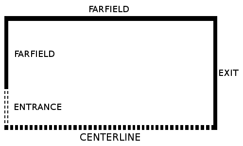
(a) Lateral view of boundary conditions.

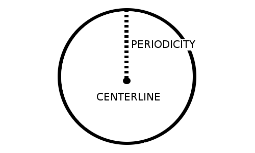
(b) Frontal view of boundary conditions.

Figure 1: Lateral and frontal views of the computational domain indicating boundary conditions.

7.1 Far Field Boundary

Riemann invariants [23] are used to implement far field boundary conditions. They are derived from the characteristic relations for the Euler equations. At the interface of the outer boundary, the following expressions apply

$$\mathbf{R}^{-}={\mathbf{R}}_{\infty}^{-} = q_{n_{\infty}}-\frac{2}{\gamma-1}a_{\infty}\,\mbox{,}$$ (74)

$$\mathbf{R}^{+}={\mathbf{R}}_{e}^{+} = q_{n_{e}}-\frac{2}{\gamma-1}a_{e}\,\mbox{,}$$ (75)

where $\infty$ and $e$ indexes stand for the property in the freestream and in the internal region, respectively. $q_{n}$ is the velocity component normal to the outer surface, defined as

$$q_{n}={\bf u}\cdot\vec{n}\,\mbox{,}$$ (76)

and $\vec{n}$ is the unit outward normal vector

$$\vec{n}=\frac{1}{\sqrt{\eta_{x}^{2}+\eta_{y}^{2}+\eta_{z}^{2}}}[\eta_{x}\ \eta_{y}\ \eta_{z}]^{T}\,\mbox{.}$$ (77)

Equation (76) assumes that the $\eta$ direction is pointing from the jet to the external boundary. Solving for $q_{n}$ and $a$, one can obtain

$$q_{nf}=\frac{\mathbf{R}^{+}+\mathbf{R}^{-}}{2}\,\mbox{,} a_{f}=\frac{\gamma-1}{4}(\mathbf{R}^{+}-\mathbf{R}^{-})\,\mbox{.}$$ (78)

The index $f$ is linked to the property at the boundary surface and will be used to update the solution at this boundary. For a subsonic exit boundary, $0<q_{n_{e}}/a_{e}<1$, the velocity components are derived from internal properties as

$$u_{f} = u_{e}+(q_{nf}-q_{n_{e}})\eta_{x}\,\mbox{,}$$

$$v_{f} = v_{e}+(q_{nf}-q_{n_{e}})\eta_{y}\,\mbox{,}$$ (79)

$$w_{f} = w_{e}+(q_{nf}-q_{n_{e}})\eta_{z}\,\mbox{.}$$

Density and pressure properties are obtained by extrapolating the entropy from the adjacent grid node,

$$\rho_{f}=\left(\frac{\rho_{e}^{\gamma}a_{f}^{2}}{\gamma p_{e}}\right)^{\frac{1}{\gamma-1}}\,\mbox{,} p_{f}=\frac{\rho_{f}a_{f}^{2}}{\gamma}\,\mbox{.}$$

For a subsonic entrance, $-1<q_{n_{e}}/a_{e}<0$, properties are obtained similarly from the freestream variables as

$$u_{f} = u_{\infty}+(q_{nf}-q_{n_{\infty}})\eta_{x}\,\mbox{,}$$

$$v_{f} = v_{\infty}+(q_{nf}-q_{n_{\infty}})\eta_{y}\,\mbox{,}$$ (80)

$$w_{f} = w_{\infty}+(q_{nf}-q_{n_{\infty}})\eta_{z}\,\mbox{,}$$

$$\rho_{f}=\left(\frac{\rho_{\infty}^{\gamma}a_{f}^{2}}{\gamma p_{\infty}}\right)^{\frac{1}{\gamma-1}}\,\mbox{.}$$ (81)

For a supersonic exit boundary, $q_{n_{e}}/a_{e}>1$, the properties are extrapolated from the interior of the domain as

$$\rho_{f} = \rho_{e}\,\mbox{,}$$

$$u_{f} = u_{e}\,\mbox{,}$$

$$v_{f} = v_{e}\,\mbox{,}$$ (82)

$$w_{f} = w_{e}\,\mbox{,}$$

$$e_{f} = e_{e}\,\mbox{,}$$

and for a supersonic entrance, $q_{n_{e}}/a_{e}<-1$, the properties are extrapolated from the freestream variables as

$$\rho_{f} = \rho_{\infty}\,\mbox{,}$$

$$u_{f} = u_{\infty}\,\mbox{,}$$

$$v_{f} = v_{\infty}\,\mbox{,}$$ (83)

$$w_{f} = w_{\infty}\,\mbox{,}$$

$$e_{f} = e_{\infty}\,\mbox{.}$$

7.2 Entrance Boundary

For a jet-like configuration, the entrance boundary is divided in two areas: the jet and the area above it. The jet entrance boundary condition is implemented through the use of the 1-D characteristic relations for the 3-D Euler equations for a flat velocity profile. The set of properties then determined is computed from within and from outside the computational domain. For the subsonic entrance, the $v$ and $w$ components of the velocity are extrapolated by a zero-order extrapolation from inside the computational domain and the angle of flow entrance is assumed fixed. The rest of the properties are obtained as a function of the jet Mach number, which is a known variable.

$$\left(u\right)_{1,j,k} = u_{j}\,\mbox{,}$$

$$\left(v\right)_{1,j,k} = \left(v\right)_{2,j,k}\,\mbox{,}$$ (84)

$$\left(w\right)_{1,j,k} = \left(w\right)_{2,j,k}\,\mbox{.}$$

The dimensionless total temperature and total pressure are defined with the isentropic relations:

$$T_{t}=1+\frac{1}{2}(\gamma-1)M_{\infty}^{2}\, P_{t}=\frac{1}{\gamma}(T_{t})^{\frac{\gamma}{\gamma-1}}\,\mbox{.}$$ and (85)

The dimensionless static temperature and pressure are deduced from Eq. (85), resulting in

$$\left(T\right)_{1,j,k}=\frac{T_{t}}{1+\frac{1}{2}(\gamma-1)(u^{2}+v^{2}+w^{2})_{1,j,k}}\, \left(p\right)_{1,j,k}=\frac{1}{\gamma}(T)_{1,j,k}^{\frac{\gamma}{\gamma-1}}\,\mbox{.}$$ and (86)

For the supersonic case, all conserved variables receive jet property values.

The far field boundary conditions are implemented outside of the jet area in order to correctly propagate information comming from the inner domain of the flow to the outter region of the simulation. However, in the present case, $\xi$, instead of $\eta$, as presented in the previous subsection, is the normal direction used to define the Riemann invariants.

7.3 Exit Boundary Condition

At the exit plane, the same reasoning of the jet entrance boundary is applied. This time, for a subsonic exit, the pressure is obtained from the outside and all other variables are extrapolated from the interior of the computational domain by a zero-order extrapolation. The conserved variables are obtained as

$$(\rho)_{I_{MAX},j,k} = \frac{(p)_{I_{MAX},j,k}}{(\gamma-1)(e)_{I_{MAX}-1,j,k}}\mbox{,}$$ (87)

$$(\vec{u})_{I_{MAX},j,k} = (\vec{u})_{I_{MAX}-1,j,k}\mbox{,}$$ (88)

$$(e_{i})_{I_{MAX},j,k} = (\rho)_{I_{MAX},j,k}\left[(e)_{I_{MAX}-1,j,k}+\frac{1}{2}(\vec{u})_{I_{MAX},j,k}\cdot(\vec{u})_{I_{MAX},j,k}\right]\,\mbox{,}$$ (89)

in which $I_{MAX}$ stands for the last point of the mesh in the axial direction. For the supersonic exit, all properties are extrapolated from the interior domain.

7.4 Centerline Boundary Condition

The centerline boundary is a singularity of the coordinate transformation, and, hence, an adequate treatment of this boundary must be provided. The conserved properties are extrapolated from the ajacent longitudinal plane and are averaged in the azimuthal direction in order to define the updated properties at the centerline of the jet.

The fourth-difference terms of the artificial dissipation scheme, used in the present work, are carefully treated in order to avoid the five-point difference stencils at the centerline singularity. If one considers the flux balance at one grid point near the centerline boundary in a certain coordinate direction, let $w_{j}$ denote a component of the $\mathcal{W}$ vector from Eq. (67) and $\mathbf{d}_{j}$ denote the corresponding artificial dissipation term at the mesh point $j$. In the present example, $\left(\Delta w\right)_{j+\frac{1}{2}}$ stands for the difference between the solution at the interface for the points $j+1$ and $j$. The fouth-difference of the dissipative fluxes from Eq. (6.1) can be written as

$$\mathbf{d}_{j+\frac{1}{2}}=\left(\Delta w\right)_{j+\frac{3}{2}}-2\left(\Delta w\right)_{j+\frac{1}{2}}+\left(\Delta w\right)_{j-\frac{1}{2}}\,\mbox{.}$$ (90)

Considering the centerline and the point $j=1$, as presented in Fig. 2, the calculation of $\mathbf{d}_{1+\frac{1}{2}}$ demands the $\left(\Delta w\right)_{\frac{1}{2}}$ term, which is unknown since it is outside the computation domain. In the present work a extrapolation is performed and given by

$$\left(\Delta w\right)_{\frac{1}{2}}=-\left(\Delta w\right)_{1+\frac{1}{2}}\,\mbox{.}$$ (91)

This extrapolation modifies the calculation of $\mathbf{d}_{1+\frac{1}{2}}$ that can be written as

$$\mathbf{d}_{j+\frac{1}{2}}=\left(\Delta w\right)_{j+\frac{3}{2}}-3\left(\Delta w\right)_{j+\frac{1}{2}}\,\mbox{.}$$ (92)

The approach is plausible since the centerline region is smooth and does not have high gradient of properties.

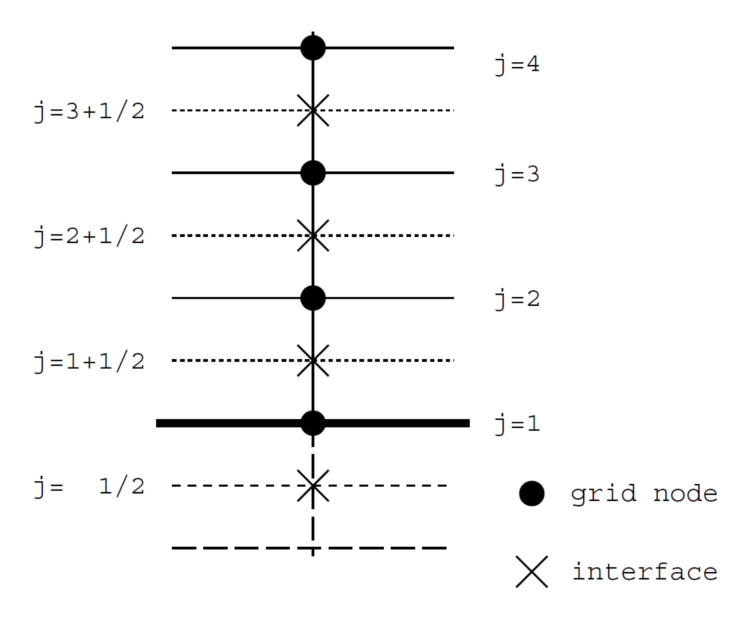
Figure 2: Boundary points dissipation [19].

7.5 Periodic Boundary Condition

A periodic condition is implemented between the first ($K=1$) and the last point in the azimutal direction ($K=K_{MAX}$) in order to close the 3-D computational domain. There are no boundaries in this direction, since all the points are inside the domain. The first and the last points, in the azimuthal direction, are superposed in order to facilitate the boundary condition implementation which is given by

$$(\rho)_{i,j,K_{MAX}} = (\rho)_{i,j,1}\,\mbox{,}$$

$$(u)_{i,j,K_{MAX}} = (u)_{i,j,1}\,\mbox{,}$$

$$(v)_{i,j,K_{MAX}} = (v)_{i,j,1}\,\mbox{,}$$ (93)

$$(w)_{i,j,K_{MAX}} = (w)_{i,j,1}\,\mbox{,}$$

$$(e)_{i,j,K_{MAX}} = (e)_{i,j,1}\,\mbox{.}$$

8 Study of Supersonic Jet Flow

Four numerical studies are performed in the present research in order to study the use of 2nd-order spatial discretization on large eddy simulations of a perfectly expanded jet flow configuration. The effects of mesh refinement and SGS models are compared in the present work. Two different meshes are created for the refinement study. The three SGS models implemented in the code, classic Smagorinsky, dynamic Smagorinsky and Vreman, are compared in the current section. Results are compared with analytical, numerical and experimental data from the literature [9, 24, 10].

8.1 Geometry Characteristics

Two different geometries are created for the simulations discussed in the current work. One geometry presents a cylindrical shape and the other one presents a divergent conical shape. For the sake of simplicity, the round geometry is named geometry A and the other one is named geometry B in present text. The computational domains are created in two steps. First, a 2-D region is generated. In the sequence, this region is rotated in order to generate a fully 3-D geometry. An in-house code is used for the generation of the 2-D domain of geometry A. The commercial mesh generator ANSYS^® ICEM CFD [25] is used for the 2-D domain of geometry B.

The geometry A is a cylindrical domain with radius of $20D$ and and length of $50D$. Geometry B presents a divergent form whose axis length is $40D$. The minimum and maximum heights of geometry B are $\approx 16D$ and $25D$, respectively. The zones of this geometry are created based on results from simulations using geometry A in order to refine the mesh in the shear layer region of the flow. Geometry A and geometry B are illustrated in Fig. 3 which presents a 3-D view of the two computational domains used in the current work. The geometries are colored by a time solution of the axial component of velocity of the flow.

(a) 3-D view of two XZ plans of geometry A.

(b) 3-D view of two XZ plans of geometry B.

Figure 3: 3-D view of geometries used for the LES.

8.2 Mesh Configurations

One grid is generated for each geometry used in the present study. These computational grids are named mesh A and mesh B. The second mesh is created based on results using mesh A. One illustration of the computational grids is presented in Fig. 4.

(a) 2-D view of mesh A in the XZ plan.

(b) 2-D view of mesh B in the XZ plan.

Figure 4: 2-D view of the computational meshes used in the current work.

Mesh A is created using a mesh generator developed by the research group for the cylindrical shape configuration. This computational mesh is composed by 400 points in the axial direction, 200 points in the radial direction and 180 points in the azimuthal direction, which originates 14.4 million grid points. Hyperbolic tangent functions are used for the points distribution in the radial and axial directions. Grid points are clustered near the shear layer of the jet. The mesh is coarsened towards the outer regions of the domain in order to dissipate properties of the flow far from the jet. Such mesh refinement approach can avoid reflection of information into the domain. The radial and longitudinal dimensions of the smallest distance between mesh points of the computational grid are given by $(\Delta\underline{r})_{min}=0.002D$ and $(\Delta\underline{x})_{min}=0.0126D$, respectively. This minimal spacing occurs at the shear layer of the jet and at the entrance of the computational domain. Mesh A is created based on a reference grid of Mendez et al. [9, 24].

The refined computational grid is composed by 343 points in the axial direction, 398 points in the radial direction and 360 points in the azimuthal direction, which yields approximately 50 million grid points. The 2-D mesh is generated with ANSYS^® ICEM CFD [25]. The points are allocated using different distributions in eight edges of the 2-D domain. The same coarsening approach used for mesh A is also applied for mesh B. The distance between mesh points increase towards the outer region of the domain. This procedure force the dissipation of properties far from the jet in order to avoid reflection of data into the domain. The reader can find more details about the mesh generation on the work of Junqueira-Junior [26].

8.3 Flow Configuration and Boundary Conditions

An unheated perfectly expanded jet flow is chosen to validate the LES tool. The flow is characterized by an unheated perfectly expanded inlet jet with a Mach number of $1.4$ at the domain entrance. Therefore, the pressure ratio, $PR=P_{j}/P_{\infty}$, and the temperature ratio, $TR=T_{j}/T_{\infty}$, between the jet exit and the ambient freestream conditions, are equal to one, i.e., $PR=1$ and $TR=1$. The Reynolds number of the jet is $Re=1.57\times 10^{6}$, based on the jet exit diameter. This flow configuration is chosen due to the absence of strong shocks waves. Strong discontinuities must be carefully treated using numerical approaches which are not yet implemented into the solver. Moreover, numerical and experimental data of this flow configuration are available in the literature such as the work of Mendez et al. [9, 24] and the work of Bridges and Wernet [10].

The boundary conditions discussed in section 7 are used in the simulations performed in the current thesis. Figure 1 presented a lateral view and a frontal view of the computational domain used by the simulation in where the positioning of each boundary condition is indicated. A flat-hat velocity profile, with $M=1.4$, is used at the entrance boundary. Riemann invariants are used at the farfield regions. A special singularity treatment is performed at the centerline. A periodicity is imposed in the azimuthal direction in order to create a transparency for the flow.

Properties of flow at the inlet and at the farfield regions have to be provided to the code in order to impose the boundary conditions. Density, $\rho$, temperature, $T$, velocity, $U$, Reynolds number $Re$, and specific heat at constant volume, $C_{v}$, are provided in the dimensionless form to the simulation. These properties are given by

$$\rho_{j}=1.00\,\mbox{,} \rho_{\infty}=1.00\,\mbox{,}$$

$$T_{j}=1.00\,\mbox{,} T_{\infty}=1.00\,\mbox{,}$$ (94)

$$U_{j}=1.4\,\mbox{,} U_{\infty}=0.00\,\mbox{,}$$

$$Re_{j}=1.57\times 10^{6}\,\mbox{,} C_{v}=1.786\,\mbox{,}$$

where the $j$ subscript stands for property at the jet entrance and the $\infty$ subscript stands for property at the farfield region.

8.4 Large Eddy Simulations

Four simulations are performed in the present. The objective is to study the effects of mesh refinement and to evaluate the three different SGS models included into the code. The calculations are performed in two steps. First a preliminary simulation is performed in order to achieve a statistically steady state condition. In the sequence, the simulations are run for another period in order to collect enough data for the calculation of time averaged properties of the flow and its fluctuations.

The configurations of all simulations are discussed in the current section, towards the description of the preliminary calculations which are performed in order to drive the flow to a statistically steady flow condition. Table 1 presents the operating conditions of all four numerical studies performed in the current research. Mesh A is only used on S1. The other calculations are performed using the refined grid, Mesh B. The stagnated flow condition is used as initial condition for all simulations but S3, which uses the solution of S2 after 10.15 flow through times (FTT). One flow through time is the necessary time for a particle to cross all the domain considering the inlet velocity of the jet. The dimensionless time increment used for all configurations is the biggest one which the solver can handle without diverging the solution. The static Smagorinsky model [3, 4, 5] is used on S1 and S2. The dynamic Smagorinsky model [6, 7] and the Vreman model [8] are used on S3 and S4, respectively.

The last column of Tab. 1 represents the period simulated by all numerical studies in order to achieve the statistically steady state flow condition. The choice of this period is related to the computational cost of each study. S1 is the least expensive test case studied. It uses a 14 million point mesh while the other simulations use the 50 million point grid. Therefore, S1 has been run for a longer period in order to achieve the statistically steady state condition. On the other hand, S3 is the most expensive numerical test case. The dynamic Smagorinsky SGS model, which is used by S3, needs more time per iteration when compared with the other SGS models implemented in the code. Hence, S3 has only been run for 5.86 FTT for this preliminary simulation.

Table 1: Configuration of large eddy simulations performed in the present work

Simulation	Mesh	SGS	$\Delta t$	Initial condition	FTT
S1	A	Static Smagorinsky	$2.5\times 10^{-5}$	Stagnated flow	37.8
S2	B	Static Smagorinsky	$1\times 10^{-4}$	Stagnated flow	10.15
S3	B	Dynamic Smagorinsky	$5\times 10^{-5}$	Stagnated flow	5.86
S4	B	Vreman	$1\times 10^{-4}$	S2 – 10.15 FTT	13.65

The simulations are restarted and run for another period in which data of the flow are extracted and recorded in a fixed frequency after the preliminary study. The collected data are time averaged in order to calculate mean properties of the flow and compare with the results of the numerical and experimental references.

In the present work, time averaged properties are notated as $\langle\cdot\rangle$. Table 2 presents the configuration of simulations performed in order to calculate mean flow properties. The second column presents the number of extractions performed during the simulations. Data are extracted each 0.02 dimensionless time in the present work which is equivalent to a dimensionless frequency of 50. The choice of this frequency is based on the numerical work reported in Refs. Mendez10 and Mendez12. The last two columns of Tab. 2 present the total dimensionless time simulated to calculate the mean properties.

Table 2: Time average configuration

Simulation	Nb. Extractions	Frequency	Total time
S1	2048	50	40.96 (1.14 FTT)
S2	3365	50	67.3 (2.36 FTT)
S3	2841	50	56.6 (1.98 FTT)
S4	1543	50	30.86 (1.08 FTT)

A power spectral density (PSD) of the time fluctuation of the axial component of velocity, $u^{*}$, is calculated in order to study the transient part of the flow. The PSD computation is performed using the following methodology: first, sensors are included at three different positions along the lipline of the jet ($r/D=0.5$). For each position along the lipline, 120 sensors are allocated in the azimuthal direction. Information at this direction are averaged in order eliminate azimuthal dependence. Table 3 presents the positioning of the sensors in the axial and radial directions. The choice of the positioning is based on the numerical reference of Mendez et. al. [9, 24]. In the sequence, data are extracted from the sensors in order to generate a time-dependent signal. The signal is partitioned into three equal parts and $u^{*}$ is calculated for all three partitioned signals. In the next step of the methodology, the time fluctuation signals are multiplied by a window function in order to create periodic distribution. The Hamming window function [27] is used in the present work and it is written as

$$w(n)=\alpha-\beta cos\left(\frac{2\pi n}{N-1}\right)\,\mbox{,}$$ (95)

where $\alpha=0.54$, $\beta=0.46$, $n$ stands for the time index and $N$ stands for the size of the sample. After applying the fast Fourier transformation (FFT) on the signals one can calculate the PSD of $u^{*}$. In the end, a simple average is applied on the three signals in order to have a final PSD of $u^{*}$ distribution.

Table 3: Positionig of the sensors used to collect fluctuation data

Signal	Positioning
(a)	$(X/D=0.10,r/D=0.5)$
(b)	$(X/D=0.25,r/D=0.5)$
(c)	$(X/D=1.25,r/D=0.5)$

In the present work the transient part is studied by the PSD of $u^{*}$ distribution as function of the number of Strouhal which is given by

$$St(t)=\frac{\mathit{f}(t)D}{U_{j}}\,\mbox{,}$$ (96)

where $\mathit{f}$ stands for the frequency as a function of the time, $D$ stands for the inlet diameter and $U_{j}$ stands for the velocity of the jet at the entrance of the domain. Data are collected from the sensors using the same informations provided by Tab. 2. The minimum and maximum values of the Strouhal number for all simulations are presented in Tab. 4.

Table 4: Strouhal limits for all simulations

Simulation	${St}_{min}$	${St}_{max}$
S1	$1.74$	17.86
S2	$1.06\times 10^{-2}$	17.86
S3	$1.26\times 10^{-2}$	17.86
S4	$2.31\times 10^{-2}$	17.86

8.5 Study of Mesh Refinement Effects

Effects of mesh refinement on compressible LES using the JAZzY solver are discussed in the present section. 2-D distribution of properties and profiles of S1 and S2 are collected and compared with numerical and experimental results from the literature [9, 24, 10]. Both simulations use the same SGS model, the static Smagorinsky model [3, 4, 5]. Mesh A is used on S1 and Mesh B is used on S2. Time averaged distributions of the axial component of velocity, density and eddy viscosity are presented in the subsection along with the RMS distribution of all three components of velocity, distributions of the $\langle u^{*}v^{*}\rangle$ component of the Reynolds stress tensor and distributions of the turbulent kinetic energy, $k$. Figure 5 illustrates the positioning of surfaces and profiles extracted for all simulations performed in the current work.

Figure 5: Positioning in the computational domain of surfaces studied in the present work

Time Averaged Axial Component of Velocity

One important characteristic of a round jet flow configurations is the potential core length, $\delta_{j}^{95\%}$. The potential core, $U_{j}^{95\%}$, is defined as $95\%$ of the velocity of the jet at the inlet,

$$U_{j}^{95\%}=0.95\cdot U_{j}\,\mbox{.}$$ (97)

Therefore, the potential core length can be defined as the positioning in the centerline where $U_{j}^{95\%}$ is located.

Time averaged results of the axial component of velocity are presented in the subsection. A lateral view of $\langle U\rangle$ for S1 and S2, side by side, are presented in Fig. 6, where $U_{j}^{95\%}$ is indicated by the solid line. The positioning of surfaces is indicated in Fig. 5. Table 5 presents the size of the potential core of S1, S2 and the numerical results from Refs. Mendez10 and Mendez12, along with the relative error compared with the experimental data [10].

Table 5: Potential core length and relative error of S1 and S2.

Simulation	$\delta_{j}^{95\%}$	Relative error
S1	5.57	40%
S2	6.84	26%
Mendez et al.	8.35	8%

(a) Lateral view of $\langle U\rangle$ for S1.

(b) Lateral view of $\langle U\rangle$ for S2.

Figure 6: Lateral view of the averaged axial component of velocity, $\langle U\rangle$, for S1 and S2. (–) indicates the potential core of the jet, $U_{j}^{95\%}$.

Comparing the results, one can observe the difference in the potential core length between S1 and S2. The results of the first case present a smaller $\delta_{j}^{95\%}$ when compared to results of S2, i.e., 5,57 and 6.84, respectively. One can say that the S1 solution is over dissipative when compared to the S2 results. The jet vanishes earlier in S1. The mesh which is used in the S1 test case is very coarse when compared with the grid used for S2. This lack of resolution can generate very dissipative solutions which yield the under prediction of the potential core length. The mesh refinement reduced in 14% the relative error of S2 when compared to the experimental data.

Profiles of $\langle U\rangle$ from S1 and S2, along the mainstream direction, and the evolution of $\langle U\rangle$ along the centerline and along the lipline are compared with numerical and experimental results in Fig. 7. The centerline and the lipline are indicated as (E) and (F) in Fig. 5. The dash-point line and the solid line stand for the results of the S1 and S2 test cases, respectively, in Fig. 7. The square symbols stand for the LES results of Mendez et al. [9, 24], while the triangular symbols stand for the experimental data of Bridges and Wernet [10].

(a) $\langle U\rangle$ - X=2.5D ; $-1.5D\leq Y\leq 1.5D$

(b) $\langle U\rangle$ - X=5.0D ; $-1.5D\leq Y\leq 1.5D$

(c) $\langle U\rangle$ - X=10D ; $-1.5D\leq Y\leq 1.5D$

(d) $\langle U\rangle$ - X=15D ; $-1.5D\leq Y\leq 1.5D$

(e) $\langle U\rangle$ - Centerline - Y=0 ; $0\leq X\leq 20D$

(f) $\langle U\rangle$ - Lipline - Y=0.5D ; $0\leq X\leq 20D$

Figure 7: Profiles of averaged axial component of velocity at different positions within the computational domain. (-$\cdot$-), S1; (–), S2; ($\square$), numerical data; ($\blacktriangle$), experimental data.

The comparison of profiles indicates that distributions of $\langle U\rangle$ calculated on S1 and S2 correlates well with the references until $X=5.0D$. The $\langle U\rangle$ profile calculated with S2 at $X=10.0D$ is under predicted when compared with the reference profiles. However, it is closer to the reference when compared with the S1 results. One can notice that S1 and S2 $\langle U\rangle$ distributions along the centerline correlates with the references in the regions which the grid presents a good resolution. When the mesh spacing increases, due to the mesh coarsening in the streamwise direction, the time average axial component of velocity start to correlate poorly with the reference. The time averaged axial component of velocity calculated by S1, along the lipline, correlates better with the reference than the same property calculated on S2. The second case overestimates the magnitude of $\langle U\rangle$ until $X\approx 6.0D$.

Root Mean Square Distribution of Time Fluctuations of Axial Velocity Component

The time fluctuation part of the flow is also important to be studied. The present work evaluates the axial and radial velocity components using the root mean square. A lateral view of $u^{*}_{RMS}$ computed by S1 and S2 simulations are presented in Figs. 8(a) and 8(b), respectively. The figures indicate that the property calculated by S1 is more spread when compared with the same property computed by S2. The mesh A refinement along with the spatial discretization can generate a more dissipative solution which creates the spread effect of $u^{*}_{RMS}$ calculated by S1 when compared to the same property calculated by S2.

(a) Lateral view of $u^{*}_{RMS}$ for S1.

(b) Lateral view of $u^{*}_{RMS}$ for S2.

(c) Lateral view of $v^{*}_{RMS}$ for S1.

(d) Lateral view of $v^{*}_{RMS}$ for S2.

(e) Lateral view of $\langle u^{*}v^{*}\rangle$ for S1.

(f) Lateral view of $\langle u^{*}v^{*}\rangle$ for S2.

Figure 8: Lateral view of RMS of time fluctuation of axial component of velocity, $u_{RMS}^{*}$, RMS of time fluctuation of radial component of velocity, $v_{RMS}^{*}$ and $\langle u^{*}v^{*}\rangle$ Reynolds shear stress tensor component, for S1 and S2.

The same strategy used to compare the mean profiles of velocity is used here for the study of $u^{*}_{RMS}$. Figure 9 presents the comparison of root mean square profiles of $u^{*}$ calculated by S1 and S2 with reference results. The profile of $u^{*}_{RMS}$ calculated by S2 fits perfectly the reference profiles at $X=2.5D$. The profile calculated by S1, at the same position, presents a good correlation with numerical and experimental data. However, it does not correctly represent the two peaks of the profile. For $X=5.0D$ and $X=10.0D$ the profiles start to diverge from the reference results. At $X=15.0D$, the $u^{*}_{RMS}$ profile, calculated by S1, present a different shape and different magnitude from the reference profiles. At the same position the fluctuation profile computed by S2 reproduce the same peaks of the reference data. However, the shape of the profile is completely different from the shape of profiles calculated by the references.

(a) $u^{*}_{RMS}$ - X=2.5D ; $-1.5D\leq Y\leq 1.5D$

(b) $u^{*}_{RMS}$ - X=5.0D ; $-1.5D\leq Y\leq 1.5D$

(c) $u^{*}_{RMS}$ - X=10D ; $-1.5D\leq Y\leq 1.5D$

(d) $u^{*}_{RMS}$ - X=15D ; $-1.5D\leq Y\leq 1.5D$

(e) $u^{*}_{RMS}$ - Centerline - Y=0 ; $0\leq X\leq 20D$

(f) $u^{*}_{RMS}$ - Lipline - Y=0.5D ; $0\leq X\leq 20D$

Figure 9: Profiles of RMS of time fluctuation of axial component of velocity, $u_{RMS}^{*}$, for S1 and S2, at different positions within the computational domain. (-$\cdot$-), S1; (–), S2; ($\square$), numerical data; ($\blacktriangle$), experimental data.

Figures 9(e) and 9(f) presents the distribution of $u^{*}_{RMS}$ along the centerline and lipline of the jet. The distributions calculated by S1 and S2 are somewhat different from the results of the references. However, one can notice an upgrade on the solution when comparing S1 and S2 results. The results achieved using the more refined mesh are closer to the reference than the results obtained using mesh A.

Root Mean Square Distribution of Time Fluctuations of Radial Velocity Component

The time fluctuation of the radial component of velocity is also compared with the reference data. Distributions of root mean square of $v_{RMS}^{*}$ are presented in the subsection. Figures 8(c) and 8(d) illustrate a lateral view of the distribution of $v_{RMS}^{*}$ computed by S1 and S2, respectively. A significant divergence between the results can be easily noticed on the lateral view of the $v_{RMS}^{*}$ distribution. From $X=2.5D$ towards the exit boundary the magnitude of fluctuation calculated by S1 is much higher than the magnitude of $v_{RMS}^{*}$ computed by S2.

Four profiles of $v_{RMS}^{*}$ in the radial direction at $X=2.5D$, $X=5.0D$, $X=10.0D$ and $X=15.0D$ are presented in Fig. 10. S1 results presented a good correlation with the reference at $X=2.5D$, where only the peaks of the profile are not well represented. For all other positions on the axial direction studied in the present research the $v_{rms}^{*}$ profiles of S1 are overestimated and poorly correlates with the reference. On the other hand, $v_{RMS}^{*}$ profiles calculated using a refined grid fits very well with the results of the numerical reference at $X=2.5D$ and $X=5.0D$. At $X=10.0D$ the fluctuation profile calculated by S2 presents a better correlation with the experimental data than the numerical reference. At $X=15.0D$ the S2 does not present a good profile of $v_{RMS}^{*}$.

(a) $v^{*}_{RMS}$ - X=2.5D ; $-1.5D\leq Y\leq 1.5D$

(b) $v^{*}_{RMS}$ - X=5.0D ; $-1.5D\leq Y\leq 1.5D$

(c) $v^{*}_{RMS}$ - X=10D ; $-1.5D\leq Y\leq 1.5D$

(d) $v^{*}_{RMS}$ - X=15D ; $-1.5D\leq Y\leq 1.5D$

Figure 10: Profiles of RMS of time fluctuation of radial component of velocity, $v_{RMS}^{*}$, for S1 nd S2, at different positions within the computational domain. (-$\cdot$-), S1; (–), S2; ($\square$), numerical data; ($\triangle$), experimental data.

Component of Reynolds Stress tensor

Figures 8(e), 8(f) and 11 present lateral views and profiles of $\langle u^{*}v^{*}\rangle$ component of the Reynolds stress tensor. One can observe that the distributions of the property obtained by S1 is over dissipated when compared with results collected from S2. Comparing the profiles with the reference, one can notice that the profiles achived in S1 and S2 are really far from the numerical and experimental data. The solver has produced with succes the shape of $\langle u^{*}v^{*}\rangle$ profile. However, it fails to represent the peak of $\langle u^{*}v^{*}\rangle$ for all profiles compared.

(a) $\langle u^{*}v^{*}\rangle$ - X=2.5D ; $-1.5D\leq Y\leq 1.5D$

(b) $\langle u^{*}v^{*}\rangle$ - X=5.0D ; $-1.5D\leq Y\leq 1.5D$

(c) $\langle u^{*}v^{*}\rangle$ - X=10D ; $-1.5D\leq Y\leq 1.5D$

(d) $\langle u^{*}v^{*}\rangle$ - X=15D ; $-1.5D\leq Y\leq 1.5D$

Figure 11: Profiles of the $\langle u^{*}v^{*}\rangle$ Reynolds shear stress tensor component, for S1 and S2, at different positions within the computational domain. (-$\cdot$-), S1; (–), S2; ($\square$), numerical data; ($\triangle$), experimental data.

Time Averaged Eddy Viscosity

The effects of the mesh on the SGS modeling are also studied in the present subsection. Figure 12 presents distributions of time averaged eddy viscosity, $\langle\mu_{t}\rangle$, calculated on S1 and S2. The Smagorinsky model [3, 4, 5] is used on both simulations. This SGS closure is highly dependent on the local mesh size. One can notice that $\langle\mu_{t}\rangle$ presents higher values on the distributions obtained by S1. On the other hand, the eddy viscosity is only acting on the regions where the mesh is no longer very refined for the S2 study. The $\langle\mu_{t}\rangle$ is very low in the region where the grid spacing is small.

(a) Lateral view of $\langle\mu_{t}\rangle$ for S1.

(b) Lateral view of $\langle\mu_{t}\rangle$ for S2.

Figure 12: Lateral view and detailed view of time averaged eddy viscosity, $\langle\mu_{t}\rangle$, for S1 and S2.

The eddy viscosity can contribute to the dissipative characteristic of the simulations. Specially for meshes with low point resolution. The divergence observed on the distribution of $\langle\mu_{t}\rangle$ calculated by S1 and S2 is an example of such effect. However, it is important to notice that, even in regions where the mesh is not very refined, yet, not coarse, and where the eddy viscosity can be neglected, some distributions of properties, calculated by S2, have shown to be very dissipative when compared with the LES reference and with the experimental data. Therefore, one can state that the truncation errors originated from the second order spatial discretization, used on the simulations here performed, can easily overcome the effects of SGS modeling if the grid spacing is not small enough. The issue is very important for the structured mesh approach. Increasing mesh resolution in the region of interest expressively rises up the number of points all over the computational domain. Local refinement for structured mesh is not straight forward and the code used in the current work does not have such approach available.

Power Spectral Density

The power spectral density of time fluctuation of the axial component of velocity is studied in the present work in order to better understand the transient portion of the solution. Figure 13 presents the PSD of $u^{*}$, in $dB$, as function of the Strouhal number for S1 and S2. The signals are collected from the sensors allocated at the positions presented in Tab. 3. The PSD of $u^{*}$ are shifted of -150dB and -300dB for $X=0.25D$ and $X=1.25$, respectively, in order to separate plots.

One can observe that PSD signals obtained using S1 and S2 present a similar behavior at $X=1.25D$ on the lipline. On the other hand, it is possible to notice significant differences on the shape and on the peaks positioning for $St>1.0$ at $X=0.1D$ and $X=0.25D$. The divergence indicates that the dissipative characteristic of S1 have changed the positioning of the turbulent transition when compared with the S2 study.

Figure 13: Power spectral density of $u^{*}$ as function of the Strouhal number along the lipline of the jet. (–), S1; (–), S2. A shift of -150 dB and -300 dB has been added to the PSD in order to separate plots for $X=0.25D$ and $X=1.25D$, respectively.

8.6 Subgrid Scale Modeling Study

After the mesh refinement study the three SGS models added to the solver are compared. S2, S3 and S4 simulations are performed using the static Smagorinsky model [3, 4, 5], the dynamic Smagorinsky model [17, 7] and the Vreman model [8], respectively. The same mesh with 50 million points is used for all three simulations. The stagnated flow condition is used as intial condition for S2 and S3. A restart of S2 is used as initial condition for the S4 simulation. The configuration of the numerical studies is presented at Tab. 1. The same comparisons performed on the study of mesh refinement effects, Sec. 8.5, are performed for the SGS modeling study.

Time Averaged Axial Component of Velocity

Effects of the SGS modeling on the time averaged results of the axial component of velocity are presented in the subsection. A lateral view of $\langle U\rangle$ for S2, S3 and S4, side by side, are presented in Fig. 14, where $U_{j}^{95\%}$ is indicated by the solid line.

(a) Lateral view of $\langle U\rangle$ for S2.

(b) Lateral view of $\langle U\rangle$ for S3.

(c) Lateral view of $\langle U\rangle$ for S4.

Figure 14: Lateral view of the averaged axial component of velocity, $\langle U\rangle$, for S2, S3 and S4. (–) indicates the potential core of the jet, $U_{j}^{95\%}$.

Table 6 presents the size of the potetial core of S2, S3 and S4 and the numerical reference [9, 24] along with the relative error compared with the experimental data [10].

Table 6: Potential core length and relative error of S2, S3 and S4.

Simulation	$\delta_{j}^{95\%}$	Relative error
S2	6.84	26%
S3	6.84	26%
S4	6.28	32%
Mendez et al.	8.35	8%

Comparing the results, one cannot observe significant differences on the potential core length between S2, S3 and S4. The distribution of $\langle U\rangle$ calculated using the dynamic Smagorinky model has shown to be slightly more concentrated at the centerline region. S2 and S4 time averaged distribution of $U$ are, on some small scale, more spread than the distribution obtained by S3.

Profiles of $\langle U\rangle$ from S2, S3 and S4, along the mainstream direction, and the evolution of $\langle U\rangle$ along the centerline and, also along the lipline, are compared with numerical and experimental results in Fig. 15. The solid line, the dashed line and the circular symbol stand for the profiles of $\langle U\rangle$ computed by S2, S3 and S4, respectively. The reference data are represented by the same symbols presented in the mesh refinement study.

(a) $\langle U\rangle$ - X=2.5D ; $-1.5D\leq Y\leq 1.5D$

(b) $\langle U\rangle$ - X=5.0D ; $-1.5D\leq Y\leq 1.5D$

(c) $\langle U\rangle$ - X=10D ; $-1.5D\leq Y\leq 1.5D$

(d) $\langle U\rangle$ - X=15D ; $-1.5D\leq Y\leq 1.5D$

(e) $\langle U\rangle$ - Centerline - Y=0 ; $0\leq X\leq 20D$

(f) $\langle U\rangle$ - Lipline - Y=0.5D ; $0\leq X\leq 20D$

Figure 15: Profiles of averaged axial component of velocity at different positions within the computational domain. (–), S2; (–), S3; ($\bigcirc$), S4; ($\square$), numerical data; ($\blacktriangle$), experimental data.

The comparison of profiles indicates that distributions of $\langle U\rangle$ calculated on S2, S3 and S4 correlates well with the references until $X=5.0D$. For $X>10.0D$ all SGS models fail to predict the correct profile. One can notice that the evolution of $\langle U\rangle$ along the centerline, calculated by all three simulations, are in good agreement with the numerical and experimental reference data at the region where the mesh presents a good resolution. Moreover, the three distributions calculated using different SGS closures have presented the very similar behavior. The dynamic Smagorinsky model and the Vreman model correlates better with the experimental data for $X<5.0D$ than the classic Smagorinsky closure does. However, all simulations tend to not predict well the magnitude of $\langle U\rangle$ on the lipline when the mesh size increases, $X>5.0D$.

Root Mean Square Distribution of Time Fluctuations of Axial Velocity Component

A lateral view of $u^{*}_{RMS}$ computed by S2, S3 and S4 simulations are presented in Figs. 16(a), 16(b) and 16(c), respectively.

(a) Lateral view of $u^{*}_{RMS}$ for S2.

(b) Lateral view of $u^{*}_{RMS}$ for S3.

(c) Lateral view of $u^{*}_{RMS}$ for S4.

(d) Lateral view of $v^{*}_{RMS}$ for S2.

(e) Lateral view of $v^{*}_{RMS}$ for S3.

(f) Lateral view of $v^{*}_{RMS}$ for S4.

(g) Lateral view of $\langle u^{*}v^{*}\rangle$ for S2.

(h) Lateral view of $\langle u^{*}v^{*}\rangle$ for S3.

(i) Lateral view of $\langle u^{*}v^{*}\rangle$ for S4.

Figure 16: Lateral view of RMS of time fluctuation of axial component of velocity, $u_{RMS}^{*}$, RMS of time fluctuation of radial component of velocity, $v_{RMS}^{*}$ and $\langle u^{*}v^{*}\rangle$ Reynolds shear stress tensor component, for S2, S3 and S4.

The profiles of $u^{*}_{RMS}$ at $X=2.5D$ obtained by S2, S3 and S4 are in good agreement with the numerical reference, as one can observe in Fig. 17. However, all simulations, including the LES reference, fail to predict the peaks of $u^{*}_{RMS}$.

(a) $u^{*}_{RMS}$ - X=2.5D ; $-1.5D\leq Y\leq 1.5D$

(b) $u^{*}_{RMS}$ - X=5.0D ; $-1.5D\leq Y\leq 1.5D$

(c) $u^{*}_{RMS}$ - X=10D ; $-1.5D\leq Y\leq 1.5D$

(d) $u^{*}_{RMS}$ - X=15D ; $-1.5D\leq Y\leq 1.5D$

(e) $u^{*}_{RMS}$ - Centerline - Y=0 ; $0\leq X\leq 20D$

(f) $u^{*}_{RMS}$ - Lipline - Y=0.5D ; $0\leq X\leq 20D$

Figure 17: Profiles of RMS of time fluctuation of axial component of velocity, $u_{RMS}^{*}$, for S2, S3 and S4, at different positions within the computational domain. (–), S2; (–), S3; ($\bigcirc$), S4; ($\square$), numerical data; ($\blacktriangle$), experimental data.

At $X=5.0D$ all three simulations have difficulties to predict the peaks of the profile. Nonetheless, the results are still in good agreement with the literature. In the sequence, the profile of $u^{*}_{RMS}$ at $X=10.0D$ calculated by S2, S3 and S4 starts to diverge from the reference results. Finally, at $X=15.0D$, all SGS closures, but the dynamic Smagorinsky model, fail the predict the correct profile. S3 simulation have produced a profile of $u_{RMS}^{*}$ at $X=15.0D$ that is closer to the experimental data than the numerical reference.

All three simulations have presented overestimated distributions of $u_{RMS}^{*}$ along the centerline. However, for $10D<X<15D$, the Vreman model correctly reproduces the magnitude of $u_{RMS}^{*}$. All simulations performed in the present work have produced noisy distributions that diverge from the experimental data along the lipline. One can notice that the numerical reference has also produced an overestimated distribution of $u_{RMS}^{*}$ at $X<10D$.

Root Mean Square Distribution of Time Fluctuations of Radial Velocity Component

Effects of SGS modeling on the time fluctuation of the radial component of velocity are also compared with the reference data. Figures 16(d), 16(e) and 16(f) illustrate a lateral view of the distribution of $v_{RMS}^{*}$ computed by S2, S3 and S4, respectively. The SGS models does not significantly affect the distribution of $v_{RMS}^{*}$. All distributions calculated by S2, S3, S4 have shown similar behavior.

Four profiles of $v_{RMS}^{*}$ in the radial direction at $X=2.5D$, $X=5.0D$, $X=10.0D$ and $X=15.0D$ are presented in Fig. 18. One can observe that, for $X\leq 10.0D$, all the profiles calculated on S2, S3 and S4 are close to the reference. Moreover, the results of the static and the dynamic Smagorinsky models are in better agreement with experimental data than the LES reference. At $X=15.0D$, all simulations performed in the current work fail to predict the correct $v_{RMS}^{*}$ profile.

(a) $v^{*}_{RMS}$ - X=2.5D ; $-1.5D\leq Y\leq 1.5D$

(b) $v^{*}_{RMS}$ - X=5.0D ; $-1.5D\leq Y\leq 1.5D$

(c) $v^{*}_{RMS}$ - X=10D ; $-1.5D\leq Y\leq 1.5D$

(d) $v^{*}_{RMS}$ - X=15D ; $-1.5D\leq Y\leq 1.5D$

Figure 18: Profiles of RMS of time fluctuation of radial component of velocity, $v_{RMS}^{*}$, for S1 nd S2, at different positions within the computational domain. (–), S2; (–), S3; ($\bigcirc$), S4; ($\square$), numerical data; ($\blacktriangle$), experimental data.

Component of Reynolds Stress Tensor

Figures 16(g), 16(h) and 16(i) present lateral view and profiles of $\langle u^{*}v^{*}\rangle$ component of the Reynolds stress tensor computed using three different SGS models, respectively. One can observe that the simulation performed using different SGS models have produced very similar distributions of $\langle u^{*}v^{*}\rangle$ for the region where the mehs is refined. However, for $X>8.0D$ the properties calculated by the different SGS closures present different behavior. The spreading is not the same for S2, S3 and S4 where $X>8.0D$. Therefore, one can state that the static Smagorinsky, the dynamic Smagorinsky and the Vreman models react differently to the coarsening of the grid.

All numerical simulations performed in the present work have failed to correct predict the profiles of $\langle u^{*}v^{*}\rangle$ presented in Fig. 19. The peaks of the component of the Reynolds stress tensor does not correlate with the reference results. However, one should notice that the LES performed by the reference has also presented difficulties to calculate the same peaks. The cause of the issue could be related to an eventual lack of grid points in the radial direction. In spite of that, more studies on the subject are necessary in order to understand such behavior.

(a) $\langle u^{*}v^{*}\rangle$ - X=2.5D ; $-1.5D\leq Y\leq 1.5D$

(b) $\langle u^{*}v^{*}\rangle$ - X=5.0D ; $-1.5D\leq Y\leq 1.5D$

(c) $\langle u^{*}v^{*}\rangle$ - X=10D ; $-1.5D\leq Y\leq 1.5D$

(d) $\langle u^{*}v^{*}\rangle$ - X=15D ; $-1.5D\leq Y\leq 1.5D$

Figure 19: Profiles of the $\langle u^{*}v^{*}\rangle$ Reynolds shear stress tensor component, for S2, S3 and S4, at different positions within the computational domain. (–), S2; (–), S3; ($\bigcirc$), S4; ($\square$), numerical data; ($\blacktriangle$), experimental data.

Time Averaged Eddy Viscosity

The distribution of the eddy viscosity, $\mu_{t}$, is discussed in the current subsection. Figure 20 presents distributions of time averaged eddy viscosity calculated using different SGS models. All subgrid scale closures used in the present work, the static Smagorinsky [3, 4, 5], the dynamic Smagorinsky [6, 7] and the Vreman [8] models, are dependent of the local mesh size by design. This characteristic is exposed on the lateral view of the flow presented in Fig. 20. The SGS models are only acting in the region where mesh presents a low resolution. Near the entrance domain, where the computational grid is very refined, the eddy viscosity can be neglected.

The remark goes in the same direction of the work of Li and Wang [28], which indicates that SGS closures introduce numerical dissipation that can be used as a stabilizing mechanism. However, this numerical dissipation does not necessarily add more physics of the turbulence to the LES solution. Therefore, in the present work, the numerical truncation, which generates the dissipative characteristic of JAZzY solutions, have show to overcome the effects of the SGS modeling. The mesh need to be very fine in order to achieve good results with second order spatial discretizations. The grid refinement generates very small grid spacing. Consequently, the SGS models, which are strongly dependent on the filter width, does not affect much the solution. A LES of compressible flow configurations without the use of SGS closure would be welcome in order to complete such discussion.

(a) $\langle\mu_{t}\rangle$ - S2

(b) $\langle\mu_{t}\rangle$ - S3

(c) $\langle\mu_{t}\rangle$ - S4

Figure 20: Lateral view of time averaged eddy viscosity, $\langle\mu_{t}\rangle$, for S2, S3 and S4.

Power Spectral Density

The power spectral density of $u^{*}$ is studied in the comparison of SGS modeling. Figure 21 presents the PSD of $u^{*}$, in $dB$, as function of the Strouhal number for S2, S3 and S4. The same methodology used on the mesh refinement study is performed here. The signals of $u^{*}$ are collected from the sensors allocated in the computational domain. The signals of Fig. 21 are shifted of -150dB and -300dB for $X=0.25D$ and $X=1.25$, respectively, in order to separate plots.

One can observe that PSD signals along the lipline obtained using S2, S3 and S4 have shown the same behavior. A small difference can be noticed for higher Strouhal number for the first two sensors, located at $X=0.1D$ and $X=0.25D$. Such remark is aligned to the same discussion performed about the eddy viscosity for different SGS models. The sensors are located in the region where the mesh present excellent resolution. Therefore, the effects of the static Smagorinsky, the dynamic Smagorinsky and the Vreman models, which are strongly dependent on the filter width, can be neglected on $u^{*}$ for $X<1.25D$.

Figure 21: Power spectral density of $u^{*}$ as function of the Strouhal number along the lipline of the jet. (–), S2; (–), S3; (–), S4. A shift of -150 dB and -300 dB has been added to the PSD in order to separate plots for $X=0.25D$ and $X=1.25D$, respectively.

9 Concluding Remarks

The current work is the study on effects of different subgrid scales models on perfectly expanded supersonic jet flow configurations using centered second-order spatial discretization. A formulation based on the the System I set of equations is used in the present work. The time integration is performed using a five-steps second order Runge-Kutta scheme. Four large eddy simulations of compressible jet flows are performed in the present research using two different mesh configurations an three different subgrid scale models. Their effects on the large eddy simulation solution are compared and discussed.

The mesh refinement study has indicated that in the region where the grid presents high resolution, the simulations are in good agreement with experimental and numerical references. For the mesh with 14 million points the simulation has produced good results for $X<2.5D$ and $-1.5D<Y<0.5D$. For the other mesh, with 50 million points, the simulations provided good agreement with the literature for $X<5.0D$ and $-1.5D<Y<0.5D$. The eddy viscosity, calculated by the static Smagorinsky model, presents very low levels in the region where the results have good correlation with the results of the literature.

The refined grid used on the mesh refinement study, mesh B, is used for the comparison of SGS models effects on the results of large eddy simulations. Three compressible jet flow simulations are performed using the classic Smagorinsky model [3, 4, 5], the dynamic Smagorinsky model [6, 7] and the Vreman model [8]. All three simulations presented similar behavior. Results presented good agreement with the reference for $X<5.0D$. In the region where the grid is very fine and the results correlates well with the literature, the eddy viscosity, provided by the SGS model, is very low values. The reason is related to the fact that the SGS closures used in the current work are strongly dependent of the filter width, which is proportional to the local mesh size.

The numerical results indicated that it is possible to achieve good results using second-order spatial discretization. The mesh ought be well resolved in order to overcome the truncation errors from the low order numerical scheme. Very fine meshes originates very small filter width. Consequently, the effects of the eddy viscosity calculated by the SGS models on the solution become unimportant. The work of Li and Wang [28] have presented similar conclusions for simplified problems. The authors indicate that SGS closures introduce numerical dissipation that can be used as a stabilizing mechanism. However, this numerical dissipation does not necessarily add more physics of the turbulence to the LES solution. Simulations without the use of any SGS model are welcome and could reinforce the argument.

References

- [1] Wolf, W. R., Azevedo, J. L. F., and Lele, S. K., “Convective Effects and the Role of Quadrupole Sources for Aerofoil Aeroacoustics,” Journal of Fluid Mechanics, Vol. 708, 2012, pp. 502–538.
- [2] Vreman, A. W., Direct and Large-Eddy Simulation of the Comperssible Turbulent Mixing Layer, Ph.D. thesis, Universiteit Twente, 1995.
- [3] Smagorinsky, J., “General Circulation Experiments with the Primitive Equations: I. The Basic Experiment,” Monthly Weather Review, Vol. 91, No. 3, March 1963, pp. 99–164.
- [4] Lilly, D. K., “On the Computational Stability of Numerical Solutions of Time- Dependent Non-Linear Geophysical Fluid Dynamics Problems,” Monthly Weather Review, Vol. 93, No. 1, January 1965, pp. 11–25.
- [5] Lilly, D. K., “The Representation of Small-Scale Turbulence in Numerical Simulation Experiments,” IBM Form No. 320-1951, Proceedings of the IBM Scientific Computing Symposium on Environmental Sciences, Yorktown Heights, N.Y., 1967, pp. 195–210.
- [6] Germano, M., Piomelli, U., Moin, P., and Cabot, W. H., “A Dynamic Subgridscale Eddy Viscosity Model,” Physics of Fluids A: Fluid Dynamics, Vol. 3, No. 7, July 1991.
- [7] Moin, P., Squires, K., Cabot, W., and Lee, S., “A Dynamic Subgrid-Scale Model for Compressible Turbulence and Scalar Transport,” Physics of Fluids A: Fluid Dynamics (1989-1993), Vol. 3, No. 11, 1991, pp. 2746–2757.
- [8] Vreman, A. W., “An Eddy-Viscosity Subgrid-Scale Model for Turbulent Shear Flow: Algebraic Theory and Applications,” Physics of Fluids, Vol. 16, No. 10, October 2004.
- [9] Mendez, S., Shoeybi, M., Sharma, A., Ham, F. E., Lele, S. K., and Moin, P., “Large-Eddy Simulations of Perfectly-Expanded Supersonic Jets: Quality Assessment and Validation,” AIAA Paper No. 2010–0271, January 2010.
- [10] Bridges, J. and Wernet, M. P., “Turbulence Associated with Broadband Shock Noise in Hot Jets,” AIAA paper, Vol. 2834, 2008, pp. 2008.
- [11] Sagaut, P., Large Eddy Simulation for Incompressible Flows, Springer, 2002.
- [12] Garnier, E., Adams, N., and Sagaut, P., Large Eddy Simulation for Compressible Flows, Springer, 2009.
- [13] Deardorff, J. W., “A Numerical Study of Three-Dimensional Turbulent Channel Flow at Large Reynolds Numbers,” Journal of Fluid Mechanics, Vol. 41, part 2, 1970, pp. 453–480.
- [14] Leonard, A., “Energy Cascade in Large Eddy Simulations of Turbulent Fluid Flows,” Adv. Geophys., Vol. A18, 1974, pp. 237–48.
- [15] Clark, R. A., Ferziger, J. Z., and Reynolds, W. C., “Evaluation of subgrid-scale models using an accurately simulated turbulent flow,” Journal of Fluid Mechanics, Vol. 91, 1979, pp. 1–16.
- [16] Vreman, B., Geurts, B., and Kuerten, H., “Large-Eddy Simulation of the Turbulent Mixing Layer Using the Clarck Model,” Theoretical Computational Fluid Dynamics, Vol. 8, No. 4, 1996, pp. 309–324.
- [17] Germano, M., “Averaging Invariance of the Turbulent Equations and Similar Subgrid Scale Modeling,” Center for Turbulence Research Manuscript 116, Stanford University and NASA - Ames Research Center, 1990.
- [18] Yoshizawa, A., “Statistical Theory for Compressible Turbulent Shear Flows, with the Application to Subgrid Modeling,” Physics of Fluids, Vol. 29, No. 7, July 1986.
- [19] Bigarella, E. D. V., Three-Dimensional Turbulent Flow Over Aerospace Configurations, M.Sc. Thesis, Instituto Tecnológico de Aeronáutica, São José dos Campos, SP, Brasil, 2002.
- [20] Turkel, E. and Vatsa, V. N., “Effect of Artificial Viscosity on Three-Dimensional Flow Solutions,” AIAA Journal, Vol. 32, No. 1, 1994, pp. 39–45.
- [21] Jameson, A. and Mavriplis, D., “Finite Volume Solution of the Two-Dimensional Euler Equations on a Regular Triangular Mesh,” AIAA Journal, Vol. 24, No. 4, Apr. 1986, pp. 611–618.
- [22] Jameson, A., Schmidt, W., and Turkel, E., “Numerical Solutions of the Euler Equations by Finite Volume Methods Using Runge-Kutta Time-Stepping Schemes,” AIAA Paper 81–1259, Proceedings of the AIAA 14th Fluid and Plasma Dynamic Conference, Palo Alto, Californa, USA, June 1981.
- [23] Long, L. N., Khan, M., and Sharp, H. T., “A Massively Parallel Three-Dimensional Euler/Navier-Stokes Method,” AIAA Journal, Vol. 29, No. 5, 1991, pp. 657–666.
- [24] Mendez, S., Shoeybi, M., Sharma, A., Ham, F. E., and Moin, S. K. L. P., “Large-Eddy Simulations of Perfectly-Expanded Supersonic Jets Using an Unstructured Solver,” AIAA Journal, Vol. 50, No. 5, May 2012, pp. 1103–1118.
- [25] ANSYS, “http://www.ansys.com/,” .
- [26] Junqueira-Junior, C. A., Development of a Parallel Solver for Large Eddy Simulation of Supersonic Jet Flow, Ph.D. thesis, Instituto Tecnoógico de Aeronáutica, São José dos Campos, SP, Brazil, 2016.
- [27] Harris, F. J., “On the Use of Windows for Harmonic Analysis with the Discrete Fourier Transform,” Proceedings of the IEEE, Vol. 66, No. 1, 1978, pp. 51–83.
- [28] Li, Y. and Wang, Z. J., “A Priori and A Posteriori Evaluation of Subgrid Stress Models with the Burger´s Equation,” AIAA-2015-1283, Proceedings of 53rd AIAA Aerospace Sciences Meeting, Kissimmee, Florida, U.S.A, 2015, p. 20.