CMB power spectrum for emergent scenario and slow expansion in scalar-tensor theory of gravity

Abstract

We analyze the stability of the Einstein static universe in scalar-tensor theory of gravity, and find it can be stable against both scalar and tensor perturbations under certain conditions. By assuming the emergent scenario originating from an Einstein static state, followed by an instantaneous transition to an inflationary phase, we study and obtain the analytical approximations of the primordial power spectrum for the emergent scenario. Then, we plot the primordial power spectrum and CMB TT-spectrum of the emergent scenario and the slow expansion scenario. These figures show that both of these spectra for the slow expansion scenario are the same as that for $\Lambda$CDM, and the spectra of the emergent scenario are lower than that for $\Lambda$CDM at large scales.

I Introduction

Inflation Guth1981 ; Linde1982 ; Albrecht1982 posits an epoch very early in the universe, during which the scale factor grows exponentially with time. It can solve most of problems in the standard cosmology. The primordial scalar perturbations originating from quantum fluctuations during the inflationary epoch not only explain the cosmic microwave background radiation anisotropy but also seed the large-scale structure of the universe Mukhanov1981 ; Lewis2000 ; Bernardeau2002 . Although it achieves great success, it still suffers from the big bang singularity problem. To solve this intractable problem, some scenarios had been proposed and suggested to construct non-singular or past eternal cosmological models, such as the emergent scenario Ellis2004a ; Ellis2004b , the slow expansion scenario Piao2003 , the pre-big bang Lidsey2000 ; Gasperini2003 , the cyclic scenario Khoury2001 ; Steinhardt2002 ; Khoury2004 , the bouncing universe Molina-Paris1999 ; Peter2002 and the other nonsingular model Starobinsky1980 ; Mukhanov1981 .

In the emergent scenario, the universe is assumed to start from an Einstein static universe and then evolves into an inflationary era Ellis2004a ; Ellis2004b . Since the universe stems from an Einstein static universe in the emergent scenario, the big bang singularity is avoided. In addition, the e-folding number and the nearly scale-invariant spectral index can also be produced by the inflation of the emergent scenario Ellis2004b . Thus, the emergent scenario has drew lots of attention after it was proposed Campo2007 ; Wu2010 ; Cai2012 ; Zhang2014 ; HuangQ2015 ; Shabani2017 ; Shabani2019 ; HuangQ2020 ; Khodadi2016 ; Heydarzade2016 ; Khodadi2018 ; Labrana2019 ; Li2019 ; Bengochea2021 ; Ilyas2021 ; Khodadi2022 . For another model, namely the slow expansion scenario, the universe originates from an Einstein static universe and then enters into an epoch in which the universe expands very slowly. During this epoch, the nearly scale-invariant primordial power spectrum is provided Piao2003 . After this scenario was proposed, it has been investigated in lots of modified gravitational theories Piao1 ; Piao2 ; Piao3 ; Liu ; Liu1 ; Cai2016 ; HuangQ2019 . In the slow expansion scenario, the universe reheats after the slow expansion scenario ends. The reheating mechanism had been studied in Ref. Liu . Then, the evolution of the hot big bang cosmology begins. In addition, it was found that in the theory with nonminimal derivative coupling Cai2016 and the scalar-tensor theory HuangQ2019 , general relativity is recovered and the universe can evolve with the standard cosmology when the slow expansion ends. Similar to the emergent scenario, the big bang singularity is also avoided since the universe originates from an Einstein static universe. Since both the emergent scenario and the slow expansion scenario assume that the universe originates from an Einstein static universe and that a stable Einstein static universe must be stable against both the scalar perturbations and the tensor perturbations, to find a stable Einstein static universe becomes a crucial issue. Fortunately, it was found that a stable Einstein static universe exists in Mimetic gravity HuangQ2020 , scalar-fluid theory Bohmer2015 , non-minimal derivative coupling model Huang2018a ; Huang2018b , braneworld model Zhang2016 , Jordan-Brans-Dicke theory Huang2014 , Eddington-inspired Born-Infeld theory Li2017 , hybrid metric-Palatini gravity Bohmer2013 , GUP theory Atazadeh2017 , f(R,T) gravity Sharif2019 , f(R,T,Q) gravity Sharif2018 , massive gravity Li2019 , and so on. Thus, the big bang singularity can be solved in the theories of modified gravity by using the emergent scenario and the slow expansion scenario.

It is notable that, except for avoiding the big bang singularity, both the emergent scenario and the slow expansion scenario can produce a nearly scale-invariant primordial power spectrum, which can explain the cosmic microwave background (CMB) radiation anisotropy observed today and provide seeds for the large-scale structure of the observable Universe Lewis2000 ; Bernardeau2002 . CMB observations indicate that there exists a suppression of CMB TT-spectrum at large scales, which was first detected by COBE Smoot1992 and recently confirmed by Planck 2018 Planck2020 . This might correspond to the physics at the very earliest universe. To explain the suppression of CMB TT-spectrum at large scales, several approaches are proposed. One approach is to introduce the spatial curvature in the inflationary model Bonga2016 ; Handley2019 . Another approach is to construct some new models, such as, double inflation Feng2003 , hybrid new inflation Kawasaki2003 , pre-inflation Cicoli2014 ; Cai2015 , emergent universe Labrana2015 , pre-inflationary bounce Cai2018 , non-flat XCDM inflation model Ooba2018 , warm inflation Arya2018 , and so on. Recently, by assuming the Einstein static state as a superinflating phase Labrana2015 or a static state phase HuangQ2022a ; HuangQ2022b , the CMB TT-spectrum of the emergent scenario was studied in the framework of general relativity, and the results show that the CMB TT-spectrum is suppressed at large scales. However, it is quite unclear that whether the CMB TT-spectrum of the slow expansion scenario is also suppressed at large scales, and whether the CMB TT-spectrum can be utilized to discriminate the emergent scenario from the slow expansion scenario. To answer these questions, we will study the CMB TT-spectrum of the emergent scenario and the slow expansion scenario in the scalar-tensor theory of gravity.

The paper is organized as follows. In section II, we briefly review the field equations of the scalar-tensor theory of gravity. In section III, we study the stability conditions of the Einstein static universe. In section IV, we will give the derivation of equations of motion for perturbations. In section V, we plot the primordial power spectrum and the CMB TT-spectrum of the emergent scenario and the slow expansion scenario. Finally, our main conclusions are shown in Section VI.

II Field equations

In this paper, we consider the following scalar-tensor theory of gravity, whose action takes the following form Bergmann ; Nordtvedt ; Wagoner1970

$$S=\int d^{4}x\sqrt{-g}\Big{[}\frac{1}{2}f(\varphi)R-\frac{1}{2}\omega(\varphi)g^{\alpha\beta}\nabla_{\alpha}\varphi\nabla_{\beta}\varphi-V(\varphi)+L_{m}\Big{]},$$ (1)

where $R$ is the Ricci curvature scalar, $\varphi$ is the scalar field of scalar-tensor theory, $f(\varphi)$ and $\omega(\varphi)$ are coupling functions of scalar field, $V(\varphi)$ is the potential, and $L_{m}$ represents the Lagrangian density of a perfect fluid. Here, the coupling function $f(\varphi)$ needs to be positive for the gravitons to carry positive energy.

Varying the action (1) with respect to the metric tensor $g^{\alpha\beta}$ and the scalar field $\varphi$, we obtain

$$f(R_{\alpha\beta}-\frac{1}{2}g_{\alpha\beta}R)-\nabla_{\alpha}\nabla_{\beta}f+g_{\alpha\beta}\nabla_{\sigma}\nabla^{\sigma}f-\omega\Big{(}\nabla_{\alpha}\varphi\nabla_{\beta}\varphi-\frac{1}{2}g_{\alpha\beta}\nabla^{\sigma}\varphi\nabla_{\sigma}\varphi\Big{)}+g_{\alpha\beta}V=T_{\alpha\beta},$$ (2)

and

$$f_{\varphi}R+\omega_{\varphi}\nabla^{\sigma}\varphi\nabla_{\sigma}\varphi+2\omega\nabla_{\sigma}\nabla^{\sigma}\varphi-2V_{\varphi}=0,$$ (3)

where $f_{\varphi}$ denotes $\frac{df}{d\varphi}$.

The field equations (2) can be expressed as the standard form of general relativity $G_{\alpha\beta}=T_{\alpha\beta}^{eff}$ with a modification in the energy-momentum tensor

$$T_{\alpha\beta}^{eff}=\frac{1}{f}\Big{[}\nabla_{\alpha}\nabla_{\beta}f-g_{\alpha\beta}(\nabla_{\sigma}\nabla^{\sigma}f+V)+\omega\Big{(}\nabla_{\alpha}\varphi\nabla_{\beta}\varphi-\frac{1}{2}g_{\alpha\beta}\nabla^{\sigma}\varphi\nabla_{\sigma}\varphi\Big{)}+T_{\alpha\beta}\Big{]}.$$ (4)

We consider a homogeneous and isotropic universe described by FLRW metric

$$ds^{2}=-a^{2}(\eta)dt^{2}+a^{2}(\eta)\gamma_{ij}dx^{i}dx^{j},\quad\gamma_{ij}dx^{i}dx^{j}=\frac{dr^{2}}{1-Kr^{2}}+r^{2}(d\theta^{2}+\sin^{2}\theta d\varphi^{2}),$$ (5)

where $K=1,0,-1$ corresponds to a closed, flat and open universe, respectively. The background equation can be obtained by substituting this metric into the field equations (2), the $0-0$ component gives the Friedmann equation

$$3\mathcal{H}^{2}+3K+3\mathcal{H}\frac{f^{\prime}}{f}=\frac{1}{f}\big{(}\frac{1}{2}\omega\varphi^{\prime 2}+a^{2}V+a^{2}\rho\big{)},$$ (6)

and the $i-i$ component gives

$$2\mathcal{H}^{\prime}+\mathcal{H}^{2}+\frac{f^{\prime\prime}}{f}+\mathcal{H}\frac{f^{\prime}}{f}+K=-\frac{1}{f}\big{(}\frac{1}{2}\omega\varphi^{\prime 2}-a^{2}V+a^{2}p\big{)},$$ (7)

where ^′ denotes a derivative with respect to the conformal time $\eta$, and $\rho$ and $p$ denote the energy density and pressure of the perfect fluid with $p=(\gamma-1)\rho$. Combining Eqs. (6) and  (7), and eliminating $\rho$, one obtain

$$2\mathcal{H}^{\prime}+\frac{f^{\prime\prime}}{f}+(3\gamma-2)\Big{(}\mathcal{H}^{2}+K+\mathcal{H}\frac{f^{\prime}}{f}\Big{)}=\frac{1}{f}\Big{[}\frac{1}{2}(\gamma-2)\omega\varphi^{\prime 2}+\gamma a^{2}V\Big{]}.$$ (8)

The field equation (3) can be expressed as

$$\varphi^{\prime\prime}+2\mathcal{H}\varphi^{\prime}+\frac{1}{2\omega}\big{[}\omega_{\varphi}\varphi^{\prime 2}+2a^{2}V_{\varphi}-6(\mathcal{H}^{\prime}+\mathcal{H}^{2}+K)f_{\varphi}\big{]}=0.$$ (9)

III Einstein static universe

Both in the emergent scenario and the slow expansion scenario, the universe stems from an Einstein static universe. However, it was found that the Einstein static solution is unstable in scalar-tensor theory of gravity when the perfect fluid is pressureless matter($\gamma=1$) or radiation($\gamma=\frac{4}{3}$)  Miao2016 . So, to find a stable Einstein static solution becomes crucial for the emergent scenario and the slow expansion scenario in this theory. In order to find a stable Einstein static solution, we reanalyze the stability of the Einstein static solution by considering $0\leq\gamma\leq 2$ in scalar-tensor theory of gravity.

III.1 Static solutions

The Einstein static solution requires $a=a_{0}=constant$ and $a^{\prime}_{0}=a^{\prime\prime}_{0}=0$ which indicates $\mathcal{H}_{0}=\mathcal{H}^{\prime}_{0}=0$. And Eqs. (6) and  (7) indicate that a constant $a$ requires $\varphi=\varphi_{0}=constant$ and $\varphi^{\prime}_{0}=\varphi^{\prime\prime}_{0}=0$. Thus, for the Einstein static solution, Eqs. (8) and  (9) show

$$\frac{K}{a_{0}^{2}}=\frac{\gamma V_{0}}{(3\gamma-2)f_{0}},$$ (10)

and

$$\frac{K}{a_{0}^{2}}=\frac{V_{0\varphi}}{3f_{0\varphi}},$$ (11)

where ₀ denotes the corresponding static state value, and ${}_{0\varphi}=\Big{(}\frac{d}{d\varphi}\Big{)}_{\varphi=\varphi_{0}}$. In addition, the energy density $\rho_{0}$ is given by Eq. (6)

$$\rho_{0}=\frac{2V_{0}}{3\gamma-2}.$$ (12)

The existence conditions of Einstein static solutions require $a^{2}_{0}>0$ and $\rho^{2}_{0}>0$ which mean

$$f_{0}>0,\quad V_{0}>0,\quad\frac{2}{3}<\gamma\leq 2,\quad\frac{V_{0\varphi}}{f_{0\varphi}}>0,$$ (13)

for $K=1$ and

$$f_{0}<0,\quad V_{0}>0,\quad\frac{2}{3}<\gamma\leq 2,\quad\frac{V_{0\varphi}}{f_{0\varphi}}<0.$$ (14)

for $K=-1$.

Since a stable Einstein static universe is required to be stable against both scalar perturbations and tensor perturbations, we will analyze the stability in the following subsections.

III.2 Tensor perturbations

Since tensor perturbations are easy to analyze, we will analyze it at first and the perturbed metric is given as Bardeen1980

$$ds^{2}=-a^{2}(\eta)d\eta^{2}+a^{2}(\eta)(\gamma_{ij}+2h_{ij})dx^{i}dx^{j}.$$ (15)

Performing a harmonic decomposition for the perturbed variable $h_{ij}$, we obtain

$$h_{ij}=H_{T,klm}(t)Y_{ij,klm}(\theta^{n}).$$ (16)

Because the quantum numbers $m$ and $l$ do not enter the perturbed differential equations, the harmonic function $Y_{k}=Y_{klm}(\theta^{n})$ satisfies Harrison1967

$$\Delta Y_{k}=-\mathcal{K}^{2}Y_{k}=\Bigg{\{}\begin{array}[]{rrr}-k(k+2)Y_{k},\quad k=0,1,2,...,\quad K=+1\\ -k^{2}Y_{k},\quad\quad\quad\quad k^{2}\geq 0,\quad\quad\quad\quad K=0\\ -(k^{2}+1)Y_{k},\quad\quad k^{2}\geq 0,\quad\quad\quad K=-1\end{array}$$ (20)

where $\Delta$ represents the three-dimensional spatial Laplacian operator. Following Ref. Barrow1993 ; Barrow1995 , considering the static conditions and then substituting the perturbed metric (15) into the field equations (2), the equation of tensor perturbations becomes

$$H^{\prime\prime}_{T}+(k^{2}+2K)H_{T}=0.$$ (21)

According to this equation, we can find that $k^{2}+2K>0$ must be satisfied for any $k$ to obtain a stable solution. As a result, the Einstein static solutions are stable against the tensor perturbations for the case $K=1$.

III.3 Scalar perturbations

Since the Einstein static solutions can be stable against the tensor perturbation for $K=1$, we will analyze the stability of the static solutions under the scalar perturbations in the closed spacetime in this subsection. To achieve this goal, we take the perturbed metric in the Newtonian gauge Bardeen1980

$$ds^{2}=-a(\eta)^{2}(1-2\Psi)d\eta^{2}+a(\eta)^{2}(1+2\Phi)\gamma_{ij}dx^{i}dx^{j},$$ (22)

where $\Psi$ denotes the Bardeen potential, and $\Phi$ represents the perturbation to the spatial curvature. Similar to the tensor perturbations, considering the static conditions and substituting the perturbed metric (22) into the field equations (2) and  (3), the equation of scalar perturbations are obtained Miao2016

$$\Psi_{k}-\Phi_{k}=\frac{f_{0\varphi}}{f_{0}}\delta\varphi_{k},$$ (23)

$$-2\mathcal{K}^{2}(\Phi_{k}-\Psi_{k})-6\Phi^{\prime\prime}=\frac{2f_{0\varphi}}{f_{0}}\mathcal{K}^{2}\delta\varphi_{k}+\frac{3a^{2}_{0}(\gamma-1)\rho_{0}}{f_{0}}\Big{[}\frac{(2\mathcal{K}^{2}-6)f_{0}}{a^{2}_{0}\rho_{0}}\Phi_{k}+\frac{\mathcal{K}^{2}f_{0\varphi}}{a^{2}_{0}\rho_{0}}\delta\varphi_{k}\Big{]}$$

$$\qquad+\frac{6a^{2}_{0}[(\gamma-1)\rho_{0}-V_{0}]}{f_{0}}\Phi_{k}+\frac{3f_{0\varphi}}{f_{0}}\delta\varphi_{k}^{\prime\prime}-\frac{3a^{2}_{0}[(\gamma-1)\rho_{0}f_{0\varphi}-V_{0}f_{0\varphi}+f_{0}V_{0\varphi}]}{f_{0}^{2}}\delta\varphi_{k},$$ (24)

$$3\Phi_{k}^{\prime\prime}+(\mathcal{K}^{2}-6)\Phi_{k}-\frac{f_{0\varphi}}{f_{0}}\mathcal{K}^{2}\delta\varphi_{k}-\frac{\omega_{0}}{f_{0\varphi}}\delta\varphi_{k}^{\prime\prime}-\frac{\omega_{0}}{f_{0\varphi}}\mathcal{K}^{2}\delta\varphi_{k}+\frac{a^{2}_{0}f_{0\varphi\varphi}}{f_{0\varphi}^{2}}V_{0\varphi}\delta\varphi_{k}$$

$$\qquad\qquad\qquad\qquad\qquad\qquad\qquad\qquad\qquad\qquad\qquad\quad-\frac{a^{2}_{0}}{f_{0\varphi}}V_{0\varphi\varphi}\delta\varphi_{k}=0,$$ (25)

$$\Big{(}\frac{2\omega_{0}f_{0}}{f_{0\varphi}}+3f_{0\varphi}\Big{)}(\delta\varphi_{k}^{\prime\prime}+\mathcal{K}^{2}\delta\varphi_{k})-2a^{2}_{0}\Big{(}V_{0\varphi}-\frac{f_{0}}{f_{0\varphi}}V_{0\varphi\varphi}+\frac{f_{0}f_{0\varphi\varphi}}{f_{0\varphi}^{2}}V_{0\varphi}\Big{)}\delta\varphi_{k}$$

$$\qquad\qquad\qquad\qquad\quad+\mathcal{K}^{2}(3\gamma-4)f_{0\varphi}\delta\varphi_{k}+2f_{0}(3\gamma-4)(\mathcal{K}^{2}-3)\Phi_{k}=0.$$ (26)

Then, combining above equations, we obtain two independent equations, which can be written as

$$\Bigg{(}\begin{array}[]{r}\xi_{k}^{\prime\prime}\\ \Phi_{k}^{\prime\prime}\end{array}\Bigg{)}+\mathbf{N}\Bigg{(}\begin{array}[]{r}\xi_{k}\\ \Phi_{k}\end{array}\Bigg{)}=0,$$ (31)

where $\xi_{k}$ is defined as $\xi_{k}=\delta\varphi_{k}/f_{0}$, and $\mathbf{N}$ is a constant coefficient matrix, which is given as

$$\mathbf{N}=\Bigg{(}\begin{array}[]{rr}N_{11}\quad N_{12}\\ N_{21}\quad N_{22}\end{array}\Bigg{)}$$ (34)

where

$$N_{11}=\frac{[2\omega_{0}f_{0}+(3\gamma-1)f^{2}_{0\varphi}]\mathcal{K}^{2}+2a^{2}_{0}f_{0}V_{0\varphi\varphi}-6f_{0}f_{0\varphi\varphi}-6f^{2}_{0\varphi}}{2\omega_{0}f_{0}+3f^{2}_{0\varphi}},$$ (35)

$$N_{12}=\frac{2(3\gamma-4)(\mathcal{K}^{2}-3)f_{0\varphi}}{2\omega_{0}f_{0}+3f^{2}_{0\varphi}},$$ (36)

$$N_{21}=\frac{[(\gamma-2)\omega_{0}f_{0}f_{0\varphi}-f^{3}_{0\varphi}]\mathcal{K}^{2}+(3f_{0\varphi\varphi}-a^{2}_{0}V_{0\varphi\varphi}-2\omega_{0})f_{0}f_{0\varphi}}{2\omega_{0}f_{0}+3f^{2}_{0\varphi}},$$ (37)

$$N_{22}=\frac{[f^{2}_{0\varphi}+2(\gamma-1)\omega_{0}f_{0}]\mathcal{K}^{2}+2(2-3\gamma)\omega_{0}f_{0}-6f^{2}_{0\varphi}}{2\omega_{0}f_{0}+3f^{2}_{0\varphi}}.$$ (38)

The stability of the static solutions against the scalar perturbations are determined by the eigenvalues of the matrix $\mathbf{N}$, which are expressed as

$$\mu^{2}_{1,2}=\frac{M\pm\sqrt{N}}{2},$$ (39)

with

$$M=N_{11}+N_{22},\quad N=(N_{11}+N_{22})^{2}+4N_{12}N_{21}-4N_{11}N_{22}.$$ (40)

If the imaginary components of $\mu_{1}$ and $\mu_{2}$ are nonzero, the corresponding Einstein static solutions are unstable. So, the stability conditions can be rewritten as

$$M>0,\quad N>0,\quad M^{2}-N>0.$$ (41)

Since the homogeneous scalar perturbation corresponds to the case $\mathcal{K}^{2}=k(k+2)=0$ and the inhomogeneous ones correspond to the other case, the stable Einstein static solutions are required to be stable for all values of $k$. So, by considering the existence conditions of Einstein static solution Eq. (13) and solving the inequalities  (41), we find the Einstein static solutions can be stable under the conditions $f_{0}>0,\omega_{0}<0,V_{0}>0$ with

$$V_{0\varphi}<0,\frac{19+\sqrt{201}}{24}<\gamma\leq\frac{7}{5},-\sqrt{-\frac{(2-3\gamma)^{2}f_{0}\omega_{0}}{18(\gamma-1)}}<f_{0\varphi}<-\frac{(2-9\gamma)f_{0}\omega_{0}}{12\gamma-1},A<V_{0\varphi\varphi}<B,$$

(42)

$$V_{0\varphi}>0,\frac{19+\sqrt{201}}{24}<\gamma\leq\frac{7}{5},\frac{(2-9\gamma)f_{0}\omega_{0}}{12\gamma-1}<f_{0\varphi}<\sqrt{-\frac{(2-3\gamma)^{2}f_{0}\omega_{0}}{18(\gamma-1)}},A<V_{0\varphi\varphi}<B,$$

where

$$A=\frac{[3f_{0}f_{0\varphi\varphi}+(12-9\gamma)f^{2}_{0\varphi}+(2-3\gamma)f_{0}\omega_{0}]V_{0\varphi}}{3f_{0}f_{0\varphi}}+\sqrt{\frac{(4-3\gamma)^{2}(2f_{0}\omega_{0}+3f^{2}_{0\varphi})V^{2}_{0\varphi}}{3f^{2}_{0}}},$$

$$B=\frac{V_{0\varphi}f_{0\varphi\varphi}}{f_{0\varphi}}+\frac{2f_{0\varphi}V_{0\varphi}}{(3\gamma-2)f_{0}}.$$

As we will see in the next section, to avoid the ghost and gradient instabilities, $f_{0\varphi}>\sqrt{-\frac{2}{3}f_{0}\omega_{0}}$ (Eq. (65)) should be satisfied. As a result, the stability conditions  (III.3) is excluded, and the Einstein static solutions can be stable under the conditions  (III.3).

From the stability conditions  (III.3), we can see that the range of value $\gamma$ is extremely narrow. To make the stability conditions more intuitive, we have plotted contours of the stable regions of the homogeneous and inhomogeneous scalar perturbations in Fig. (1) by considering $f=1+\xi\varphi+\lambda\varphi^{2}$, $\omega=-\frac{w}{\varphi}$ and $V=V_{1}+\alpha\varphi+\beta\varphi^{2}$. To make sure the value of $f_{0}$, $\omega_{0}$, $V_{0\varphi}$, $\gamma$ and $f_{0\varphi\varphi}$ satisfy the stability conditions  (III.3), we take $\xi=0.05$, $\lambda=0.482$, $w=1$, $V_{1}=0.5138$, $\alpha=-0.5$, $\beta=0.7062$ and $\gamma=1.4$ as an example. In this figure, $k=0$ denotes the homogeneous scalar perturbations, and $k=2,3,4,5$ correspond to the inhomogeneous ones. For the inhomogeneous scalar perturbations, the stable region becomes larger and larger with the increase of $k$, and the stable region of $k=0$ overlaps with the case $k=5$. As a result, the region for $k=2$ is the smallest stable region which represents the stable region for the Einstein static solutions. Thus, a stable Einstein static universe can exist in the scalar-tensor theory of gravity and an example is depicted in Fig. (2) by solving Eqs. (8) and  (9) numerically under the stability conditions.

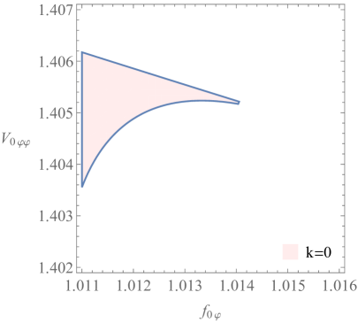
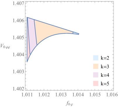
Figure 1: Stability regions in $(V_{0\varphi\varphi},f_{0\varphi})$ plane under homogeneous and inhomogeneous scalar perturbations. $k=0$ represents the homogeneous scalar perturbations while $k=2,3,4,5$ correspond to the inhomogeneous ones. These figures are plotted for $f_{0}=1.532$, $\omega_{0}=-1$, $V_{0\varphi}=0.9052$, $\gamma=1.4$ and $f_{0\varphi\varphi}=0.964$.

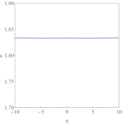
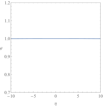
Figure 2: Evolutionary curves of scale factor $a$ and scalar field $\varphi$ under the stability conditions. These figures are plotted for $f=1+0.05\varphi+0.482\varphi^{2}$, $\omega=-\frac{1}{\varphi}$, $V=0.5138-0.5\varphi+0.7026\varphi^{2}$ and $\gamma=1.4$.

IV Perturbations

To analyze the power spectrum of the emergent scenario and the slow expansion scenario in scalar-tensor theory of gravity, we are required to obtain the equation of motion for perturbation. In this section, we will derive this equation.

IV.1 Conformal transformation to Einstein gravity

The scalar-tensor theory of gravity can be transformed into Einstein gravity by performing a conformal transformation on the metric Hwang ; Hwang1990 ; Farese ; Qiu ; Glavan2015

$$\tilde{g}_{\alpha\beta}=\Omega^{2}g_{\alpha\beta},$$ (44)

and the corresponding action becomes

$$\tilde{S}=\int d\tilde{t}d^{3}x\sqrt{-\tilde{g}}\big{(}\frac{1}{2}\tilde{R}-\frac{1}{2}\tilde{\nabla}^{\sigma}\tilde{\varphi}\tilde{\nabla}_{\sigma}\tilde{\varphi}-\tilde{V}\big{)},$$ (45)

which is the action for a minimal coupling single scalar field $\tilde{\varphi}$ and the conformal factor is $\Omega=\sqrt{f}$, and the corresponding variables are defined as

$$d\tilde{t}=\Omega dt,\quad\tilde{a}=\Omega a,\quad\tilde{\Phi}=\Phi+\delta\Omega,\quad\tilde{\Psi}=\Psi-\delta\Omega,\quad d\tilde{\varphi}=\sqrt{\frac{\omega}{f}+\frac{3}{2}\frac{f_{,\varphi}^{2}}{f^{2}}}d\varphi,\quad\tilde{V}=\frac{V}{f^{2}}.$$ (46)

Here, the Lagrangian density of a perfect fluid $L_{m}$ is ignored for the reasons: (i) The evolution of the universe is dominated by the scalar field before inflation ends. (ii) During the inflationary epoch, the scale factor of the universe increases exponentially, and the energy density of the perfect fluid becomes very small. Thus, the action (1) without the term $L_{m}$ and  (45) are fully equivalent Hwang ; Hwang1990 ; Farese ; Qiu ; Glavan2015 ; Weenink ; Prokopec2012 ; Prokopec2013 . We will discuss the cosmological perturbations in action (45) since it is easier to analyze. The background equation and the equation of motion for the field $\tilde{\varphi}$ can be written as follows

$$3\tilde{H}^{2}+3\frac{K}{\tilde{a}^{2}}=\frac{1}{2}\dot{\tilde{\varphi}}^{2}+\tilde{V},$$ (47)

$$3\tilde{H}^{2}+2\dot{\tilde{H}}+\frac{K}{\tilde{a}^{2}}=-\big{(}\frac{1}{2}\dot{\tilde{\varphi}}^{2}-\tilde{V}\big{)},$$ (48)

and

$$\ddot{\tilde{\varphi}}+3\tilde{H}\dot{\tilde{\varphi}}+\tilde{V}_{\tilde{\varphi}}=0.$$ (49)

Here, the no ghost condition $\dot{\tilde{\varphi}}^{2}>0$ gives $\omega f+\frac{3}{2}\big{(}\frac{df}{d\varphi}\big{)}^{2}>0$ which is contained in expression (64), and a dot represents the derivative with respect to the cosmic time $t$.

In order to obtain the perturbation equations with curvature $K$, we use the method developed by Garriga and Mukhanov Garriga ; Mukhanov2 . Then, the perturbation equations for $0-0$ and $0-i$ components can be written as Mukhanov ; Garriga

$$2\Big{[}\frac{1}{\tilde{a}^{2}}\Delta\tilde{\Psi}-3\tilde{H}\dot{\tilde{\Psi}}+3\big{(}\frac{K}{\tilde{a}^{2}}\tilde{\Psi}-\tilde{H}^{2}\tilde{\Phi}\big{)}\Big{]}=\dot{\tilde{\varphi}}\dot{\delta\tilde{\varphi}}-\tilde{\Phi}\dot{\tilde{\varphi}}^{2}+\tilde{V}_{\tilde{\varphi}}\delta\tilde{\varphi},$$ (50)

$$2\nabla_{i}\big{(}\dot{\tilde{\Psi}}+\tilde{H}\tilde{\Phi}\big{)}=\dot{\tilde{\varphi}}\nabla_{i}\delta\tilde{\varphi},$$ (51)

where $\Delta=\nabla^{2}$ is Laplace operator, and the component for $i\neq j$ is

$$\frac{1}{\tilde{a}^{2}}\nabla_{j}\nabla^{i}\big{(}\tilde{\Phi}-\tilde{\Psi}\big{)}=0,$$ (52)

which gives $\tilde{\Phi}=\tilde{\Psi}$. After introducing two new variables

$$\tilde{\xi}=\frac{2\tilde{a}}{\tilde{H}}\tilde{\Psi},$$ (53)

$$\tilde{\zeta}=\tilde{\Psi}+\tilde{H}\frac{\delta\tilde{\varphi}}{\dot{\tilde{\varphi}}}-\frac{2K}{\tilde{a}^{2}\dot{\tilde{\varphi}}^{2}}\tilde{\Psi},$$ (54)

the equations (51) and  (50) can be simplified as

$$\dot{\tilde{\xi}}=\tilde{a}\frac{\dot{\tilde{\varphi}}^{2}}{\tilde{H}^{2}}\tilde{\zeta},$$ (55)

$$\dot{\tilde{\zeta}}=\frac{\tilde{H}^{2}}{\tilde{a}^{3}\dot{\tilde{\varphi}}^{2}}\big{(}\Delta+YK\big{)}\tilde{\xi},$$ (56)

where

$$Y=-2\frac{\tilde{V}_{\tilde{\varphi}}}{\tilde{H}\dot{\tilde{\varphi}}}.$$ (57)

The detailed process is given in Appendix.

In order to obtain the amplitude of quantum fluctuations, one needs to expand the action for the gravitational and scalar fields to second order in perturbations which are cumbersome. Since the second order perturbation action can be inferred directly from the equations of motion (55) and  (56), these cumbersome steps can be avoided. The detailed steps are given in Ref. Garriga ; Mukhanov2 . Thus, the action reproducing the perturbation equations (55) and  (56) can be written as

$$\tilde{S}=\int\Big{[}\tilde{\xi}\tilde{O}\dot{\tilde{\zeta}}-\frac{1}{2}\frac{\tilde{H}^{2}}{\tilde{a}^{3}\dot{\tilde{\varphi}}^{2}}\tilde{\xi}\tilde{O}(\Delta+YK)\tilde{\xi}+\frac{1}{2}\frac{\tilde{a}\dot{\tilde{\varphi}}^{2}}{\tilde{H}^{2}}\tilde{\zeta}\tilde{O}\tilde{\zeta}\Big{]}d\tilde{t}d^{3}x,$$ (58)

where $\tilde{O}=\Delta+3K$ is a time-independent operator. Expressing $\tilde{\xi}$ in terms of $\dot{\tilde{\zeta}}$ by equation (56), the action can be reduced to

$$\tilde{S}=\int z^{2}\big{[}\tilde{\zeta}^{\prime 2}+\tilde{\zeta}(\Delta+YK)\tilde{\zeta}\big{]}d\eta d^{3}x,$$ (59)

where prime denotes the derivative with respect to the conformal time $\eta$, and the variable $z$ is

$$z=\frac{\tilde{a}\tilde{\varphi^{\prime}}}{\mathcal{\tilde{H}}}\sqrt{\frac{\tilde{O}}{\Delta+YK}}.$$ (60)

The Laplacian $\Delta$ should be understood as a $c-number$ and represents the corresponding eigenvalue.

IV.2 Equation of motion for perturbation

The second perturbation action in the scalar-tensor theory of gravity can be obtained by a transformation for the action (59). Introducing the canonical quantization variable $v=z\tilde{\zeta}$ and utilizing the corresponding transform equations (46), the action (59) can be rewritten as follows

$$S=\frac{1}{2}\int\Big{[}v^{\prime 2}+v(\Delta+YK)v+\frac{z^{\prime\prime}}{z}v^{2}\Big{]}d\eta d^{3}x.$$ (61)

Here, $z$ and $Y$ are

$$z=\frac{a^{2}\varphi^{\prime}\sqrt{E}}{(a\sqrt{f})^{\prime}}\sqrt{\frac{\Delta+3K}{\Delta+YK}},$$ (62)

and

$$Y=2\frac{(a^{2}\varphi^{\prime}\sqrt{E})^{\prime}/(a^{2}\varphi^{\prime}\sqrt{E})}{(a\sqrt{f})^{\prime}/(a\sqrt{f})},$$ (63)

where

$$E=f\Big{(}\omega+\frac{3}{2}\frac{f^{2}_{\varphi}}{f}\Big{)}.$$ (64)

To avoid the ghost and gradient instabilities, $f>0$ and $E>0$ should be satisfied. In previous section, we find $f_{0}>0$ and $\omega_{0}<0$ (Eqs. (III.3) and  (III.3)) are required to obtain a stable Einstein static universe. Under the conditions $f_{0}>0$ and $\omega_{0}<0$, the constraint condition $E>0$ gives

$$f_{0\varphi}>\sqrt{-\frac{2}{3}f_{0}\omega_{0}}.$$ (65)

Taking this condition  (65) into consideration, the stability conditions  (III.3) are excluded. Thus, when the conditions  (III.3) are satisfied, the Einstein static universe is stable and there is no the ghost and gradient instabilities.

Varying the action (61) with respect to $v$, one can straightforwardly get the equation of motion for the variable as

$$v^{\prime\prime}-(\Delta+YK)v-\frac{z^{\prime\prime}}{z}v=0.$$ (66)

Expressing $\tilde{\zeta}$ and $\dot{\tilde{\zeta}}$ in the action (58) in terms of $\tilde{\dot{\xi}}$ and $\tilde{\xi}$, we obtain

$$u^{\prime\prime}-(\Delta+YK)u-\frac{Z^{\prime\prime}}{Z}u=0,$$ (67)

where

$$u=\frac{a\sqrt{f^{3}}}{\varphi^{\prime}\sqrt{E}}\tilde{\psi},\quad Z=\frac{(a\sqrt{f})^{\prime}}{a^{2}\varphi^{\prime}\sqrt{E}}.$$ (68)

The equation of motion for the variable $u$ was obtained in Ref. Hwang1 ; Hwang1991 by doing some calculations.

V CMB power spectrum

In order to discuss whether the CMB TT-spectrum can discriminate the emergent scenario from the slow expansion scenario, we study the primordial power spectrum and the CMB TT-spectrum of the emergent scenario and the slow expansion scenario in this section.

V.1 Emergent scenario

In emergent scenario, the universe stems from an Einstein static state, and then evolves into an inflationary epoch Ellis2004a ; Ellis2004b . To realize this transition, there exist two different approaches: (i) assuming the Einstein static state defined by $a^{\prime}=0$ and then invoking an instantaneous transition to the inflationary epoch Wu2010 ; HuangQ2015 . (ii) considering the evolution of the scale factor as $a(t)=a_{0}+Ae^{H_{0}t}$ Ellis2004a ; Ellis2004b . In our previous work HuangQ2022a , we found that both approaches produce the same CMB TT-spectra. So, in this section, we will adopt the first approach.

Following Ref. HuangQ2022a ; Thavanesan2021 ; Shumaylov2022 , considering the Einstein static conditions, the scale factor in Einstein static state $a_{0}$ is given by Eq. (10). During this epoch, the variable $Y$ and $z$ in Eqs. (63) and  (62) reduce to

$$Y\approx 0,\quad z\approx 0.$$ (69)

So, the equation of motion for the variable $v$ (Eq. (66)) can be written as

$$v^{\prime\prime}_{k}+k^{2}_{-}v_{k}=0,\quad k^{2}_{-}=k(k+2),$$ (70)

which has the solution

$$v_{k}(\eta)=\sqrt{\frac{1}{2k}}e^{-ik_{-}\eta},$$ (71)

where the normalization conditions $v_{k}v_{k}^{*^{\prime}}-v^{{}^{\prime}}_{k}v_{k}^{*}=i$ and the Bunch-Davies vacuum are considered.

In slow-roll region, using the slow-roll conditions $f^{\prime\prime}\ll\mathcal{H}f^{\prime}\ll\mathcal{H}^{2}f$ and $\varphi^{\prime 2}\ll a^{2}V$  Barrow1995a , Eqs. (6) and  (7) reduces to

$$\mathcal{H}^{\prime}-\mathcal{H}-1\approx 0,$$ (72)

which has the solution

$$a=\frac{a_{0}}{\cos(\eta-\eta_{t})}.$$ (73)

Thus, the scale factor for the emergent scenario can be expressed as

$$a(\eta)=\Bigg{\{}\begin{array}[]{ll}a_{0},&\eta<\eta_{t}\\ \frac{a_{0}}{\cos(\eta-\eta_{t})},&\eta_{t}\leq\eta<\eta_{t}+\frac{\pi}{2},\end{array}$$ (76)

which is also obtained in general relativity HuangQ2022a ; HuangQ2022b . With $\eta$ approaching to $\eta_{t}+\frac{\pi}{2}$, the universe freezes out into the inflationary phase. The evolutionary curve of scale factor $a_{0}$ is shown in Fig. (3), the purple point denotes the transition point. To realize this transition, one can break the stability conditions by considering the scalar potential or the equation of state varying with conformal time $\eta$ slowly Wu2010 ; HuangQ2015 ; HuangQ2020 . Once $\eta$ evolves to a critical point, the stability conditions will break down automatically.

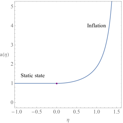
Figure 3: Evolutionary curve of scale factor $a$. The scale factor in the Einstein static state has been chosen as $a_{0}=1$ and the purple point denotes the transition point.

During the slow-roll region, the variable $Y$ and $z$ reduce to

$$Y\approx 4,\quad z\approx\frac{a\varphi^{\prime}\sqrt{\omega}}{\mathcal{H}}\sqrt{\frac{k(k+2)+3}{k(k+2)+4}}.$$ (77)

So, the equation of motion for the variable $v$ (Eq. (66)) becomes

$$v^{\prime\prime}_{k}+\Big{\{}k^{2}_{+}-\frac{2}{\big{[}\eta-(\eta_{t}+\frac{\pi}{2})\big{]}^{2}}\Big{\}}v_{k}=0,\quad k^{2}_{+}=k(k+2)-\frac{17}{3},$$ (78)

which has the solution taking the form

$$v_{k}(\eta)=\sqrt{\frac{\pi}{4}}\sqrt{\big{(}\eta_{t}+\frac{\pi}{2}\big{)}-\eta}\Big{[}C_{k}H^{(1)}_{3/2}\Big{(}k_{+}\big{(}(\eta_{t}+\frac{\pi}{2})-\eta\big{)}\Big{)}+D_{k}H^{(2)}_{3/2}\Big{(}k_{+}\big{(}(\eta_{t}+\frac{\pi}{2})-\eta\big{)}\Big{)}\Big{]},$$ (79)

where $H^{(1)}$ and $H^{(2)}$ are the Hankel functions of the first and second kinds.

To determine $C_{k}$ and $D_{k}$, we use the continuity condition of $v_{k}$ and $v^{\prime}_{k}$ to match Eqs. (71) and  (79) at the transition time $\eta_{t}$ and obtain

$$C_{k}=\frac{1}{4}e^{-ik_{-}\eta_{t}}\sqrt{\frac{1}{k_{-}}}\Big{[}i\pi k_{+}H^{(2)}_{1/2}\Big{(}\frac{\pi}{2}k_{+}\Big{)}+(-2i+\pi k_{-})H^{(2)}_{3/2}\Big{(}\frac{\pi}{2}k_{+}\Big{)}\Big{]},$$ (80)

$$D_{k}=-\frac{1}{4}e^{-ik_{-}\eta_{t}}\sqrt{\frac{1}{k_{-}}}\Big{[}i\pi k_{+}H^{(1)}_{1/2}\Big{(}\frac{\pi}{2}k_{+}\Big{)}+(-2i+\pi k_{-})H^{(1)}_{3/2}\Big{(}\frac{\pi}{2}k_{+}\Big{)}\Big{]}.$$ (81)

The curved primordial power spectrum of the comoving curvature perturbation $\mathcal{R}$ is defined as

$$\mathcal{P}_{\mathcal{R}}=\frac{k^{3}}{2\pi^{2}}\left|\mathcal{R}_{k}\right|^{2}=\frac{k^{3}}{2\pi^{2}}\left|\frac{v_{k}}{z_{k}}\right|^{2}.$$ (82)

Then, substituting Eq. (79) into Eq. (82), we obtain the curved primordial power spectrum of $\mathcal{R}$

$$\mathcal{P}_{\mathcal{R}} =\frac{k^{3}}{2\pi^{2}}\left|\mathcal{R}_{k}\right|^{2}\approx\lim_{\eta\rightarrow\eta_{t}+\frac{\pi}{2}}\frac{1}{4\pi^{2}}\frac{1}{\frac{a^{2}\varphi^{\prime 2}\omega}{\mathcal{H}}\frac{k(k+2)+3}{k(k+2)+4}}\frac{k^{3}}{k^{3}_{+}}\frac{1}{\big{[}\eta-(\eta_{t}+\frac{\pi}{2})\big{]}^{2}}\left|C_{k}-D_{k}\right|^{2}$$ (83)

$$=A_{s}\frac{k^{3}}{k^{3}_{+}}\frac{k(k+2)+3}{k(k+2)+4}\left|C_{k}-D_{k}\right|^{2},$$

where formally diverging parameters are absorbed into the usual scalar power spectrum amplitude $A_{s}$ Thavanesan2021 ; Shumaylov2022 . And the analytical primordial power spectrum can be parameterized as

$$\mathcal{P}_{\mathcal{R}}=A_{s}\Big{(}\frac{k}{k_{*}}\Big{)}^{n_{s}-1}\frac{k^{3}}{k^{3}_{+}}\frac{k(k+2)+3}{k(k+2)+4}\left|C_{k}-D_{k}\right|^{2},$$ (84)

where $k_{*}=0.05Mpc^{-1}$ corresponds to the pivot perturbation mode.

V.2 Slow expansion scenario

In slow expansion scenario, the universe also stems from an Einstein static state, and then evolves into a slowly expanded epoch which can generate the scale invariant primordial power spectrum Piao2003 . In scalar-tensor theory of gravity, by considering $f(\varphi)=1-\xi\varphi+\lambda\varphi^{2}$, $\omega(\varphi)=\omega_{0}\varphi^{-1}$ and $V(\varphi)=-V_{0}\varphi^{\frac{3}{2}}$, the slow expansion scenario was analyzed and it was found that the analytical primordial power spectrum is scale invariant and has the form HuangQ2019

$$\mathcal{P}_{\mathcal{R}}=\frac{k^{3}}{2\pi^{2}}\left|\frac{v_{k}}{z_{k}}\right|^{2}\approx\frac{V_{0}\xi^{\frac{5}{2}}}{128\pi^{2}}=A_{s}.$$ (85)

Parameterizing this primordial power spectrum, it can be written as

$$\mathcal{P}_{\mathcal{R}}=A_{s}\Big{(}\frac{k}{k_{*}}\Big{)}^{n_{s}-1},$$ (86)

which is the same as that in $\Lambda$CDM model.

V.3 Power spectrum

To plot the primordial power spectrum in the closed universe, we use the Planck 2018 results in the curved universes best-fit data (TT,TE,EE+lowl+lowE+lensing) $A_{s}=2.0771\pm 0.1017\times 10^{-9}$ and $n_{s}=0.9699\pm 0.0090$. For the flat universe, the Planck 2018 results in Ref. Planck2020 is adopted. In the left panel of Fig. (4), we have plotted the primordial power spectrum for $\Lambda$CDM, K$\Lambda$CDM, the emergent scenario and the slow expansion scenario. This figure shows that the primordial power spectra of the slow expansion scenario and $\Lambda$CDM are overlapped. Comparing to $\Lambda$CDM, K$\Lambda$CDM and the slow expansion scenario, the primordial power spectrum of emergent scenario oscillates and is suppressed during the region $k<100$.

Then, using CLASS code Blas2011 , we have depicted the CMB TT-spectrum in the right panel of Fig. (4). From this figure, we can see that the CMB TT-spectrum of the slow expansion scenario is the same as that in $\Lambda$CDM, and the CMB TT-spectrum of emergent scenario is lower than the one in $\Lambda$CDM for $l<10$. Thus, comparing to the slow expansion scenario, the emergent scenario can produce a lower CMB TT-spectrum at large scales.

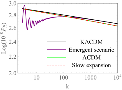
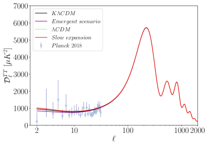
Figure 4: Primordial power spectrum and CMB TT-spectrum for the emergent scenario and the slow expansion scenario.

VI Conclusion

The scalar-tensor theory is an extension of general relativity by coupling a scalar field $\varphi$ to the Ricci scalar $R$ with terms $f(\varphi)R$, and it can be expressed as general relativity with a modified energy-momentum tensor. In this paper, we study the primordial power spectrum and CMB TT-spectrum of the emergent scenario and the slow expansion scenario in the scalar-tensor theory of gravity. Since both in the emergent scenario and in the slow expansion scenario, the universe stems from an Einstein static universe, we analyze the stability of the Einstein static universe in scalar-tensor theory of gravity at first, and find the Einstein static universe can be stable against both scalar and tensor perturbations under the certain conditions.

Assuming the emergent scenario starts from an Einstein static universe followed by an instantaneous transition to an inflationary phase, we study the primordial power spectrum for the emergent scenario and obtain the analytical approximations of this spectrum. To comparing the primordial power spectrum and CMB TT-spectrum of the emergent scenario and the slow expansion scenario, we have plotted these spectra by using Planck 2018 results. These figures show that both of these spectra for the slow expansion scenario are the same as the one in $\Lambda$CDM, and the spectra of the emergent scenario are lower than the one in $\Lambda$CDM at large scales. Thus, comparing to the slow expansion scenario, the emergent scenario can produce a lower CMB TT-spectrum at large scales.

VII Appendix

Equation (51) can be written as

$$(\tilde{a}\tilde{\Psi})^{.}=\frac{1}{2}\tilde{a}\dot{\tilde{\varphi}}^{2}\big{(}\frac{\delta\tilde{\varphi}}{\dot{\tilde{\varphi}}}\big{)},$$ (87)

and expressing $\frac{\delta\tilde{\varphi}}{\dot{\tilde{\varphi}}}$ and $\tilde{\Psi}$ in terms of $\tilde{\zeta}$ and $\tilde{\xi}$, one obtains

$$\dot{\tilde{H}}\tilde{\xi}+\tilde{H}\dot{\tilde{\xi}}=\tilde{a}\dot{\tilde{\varphi}}^{2}\Big{[}\frac{\tilde{\zeta}}{\tilde{H}}-\Big{(}\frac{1}{2\tilde{a}}-\frac{K}{\tilde{a}^{3}\dot{\tilde{\varphi}}^{2}}\Big{)}\tilde{\xi}\Big{]}=\tilde{a}\dot{\tilde{\varphi}}^{2}\frac{\tilde{\zeta}}{\tilde{H}}-\Big{(}\frac{\dot{\tilde{\varphi}}^{2}}{2}-\frac{K}{\tilde{a}^{2}}\Big{)}\tilde{\xi}.$$ (88)

Then, using the equation $\dot{\tilde{H}}-\frac{K}{\tilde{a}^{2}}=-\frac{1}{2}\dot{\tilde{\varphi}}^{2}$ obtained from the background equation (47) and  (48), one gets

$$\dot{\tilde{\xi}}=\tilde{a}\frac{\dot{\tilde{\varphi}}^{2}}{\tilde{H}^{2}}\tilde{\zeta},$$ (89)

Equation (50) can be written as

$$\frac{1}{\tilde{a}^{2}}(\Delta+3K)\tilde{\Psi}-3\tilde{H}(\dot{\tilde{\Psi}}+\tilde{H}\tilde{\Phi})=\frac{1}{2}\Big{[}\dot{\tilde{\varphi}}\dot{\delta\tilde{\varphi}}-\tilde{\Phi}\dot{\tilde{\varphi}}^{2}-\Big{(}\dot{\tilde{\varphi}}\ddot{\tilde{\varphi}}+3\tilde{H}\dot{\tilde{\varphi}}^{2}\Big{)}\frac{1}{\dot{\tilde{\varphi}}}\delta\tilde{\varphi}\Big{]}$$ (90)

$$=\frac{1}{2}\Big{[}-\dot{\tilde{\varphi}}^{2}\Big{(}\tilde{\Phi}-\dot{\tilde{\varphi}}\frac{\dot{\delta\tilde{\varphi}}}{\dot{\tilde{\varphi}}^{2}}+\ddot{\tilde{\varphi}}\frac{\delta\tilde{\varphi}}{\dot{\tilde{\varphi}}^{2}}\Big{)}-3\tilde{H}\dot{\tilde{\varphi}}^{2}\frac{\delta\tilde{\varphi}}{\dot{\tilde{\varphi}}}\Big{]}$$

$$=-\frac{1}{2}\Big{\{}\dot{\tilde{\varphi}}^{2}\Big{[}\tilde{\Phi}-\Big{(}\frac{\delta\tilde{\varphi}}{\dot{\tilde{\varphi}}}\Big{)}^{.}\Big{]}+3\tilde{H}\dot{\tilde{\varphi}}^{2}\Big{(}\frac{\delta\tilde{\varphi}}{\dot{\tilde{\varphi}}}\Big{)}\Big{\}},$$

$$\frac{1}{\tilde{a}^{2}}(\Delta+3K)\tilde{\Psi}=\frac{1}{2}\dot{\tilde{\varphi}}^{2}\Big{[}\Big{(}\frac{\delta\tilde{\varphi}}{\dot{\tilde{\varphi}}}\Big{)}^{.}-\tilde{\Psi}\Big{]}-\frac{3}{2}\tilde{H}\dot{\tilde{\varphi}}^{2}\big{(}\frac{\delta\tilde{\varphi}}{\dot{\tilde{\varphi}}}\Big{)}+3\tilde{H}(\dot{\tilde{\Psi}}+\tilde{H}\tilde{\Psi})$$ (91)

$$=\frac{1}{2}\dot{\tilde{\varphi}}^{2}\Big{[}\Big{(}\frac{\delta\tilde{\varphi}}{\dot{\tilde{\varphi}}}\Big{)}^{.}-\tilde{\Psi}\Big{]}-\frac{3}{2}\tilde{H}\dot{\tilde{\varphi}}^{2}\big{(}\frac{\delta\tilde{\varphi}}{\dot{\tilde{\varphi}}}\Big{)}+3\tilde{H}\Big{[}\frac{1}{2}\dot{\tilde{\varphi}}^{2}\Big{(}\frac{\delta\tilde{\varphi}}{\dot{\tilde{\varphi}}}\Big{)}\Big{]}$$

$$=\frac{1}{2}\dot{\tilde{\varphi}}^{2}\Big{[}\Big{(}\frac{\delta\tilde{\varphi}}{\dot{\tilde{\varphi}}}\Big{)}^{.}-\tilde{\Psi}\Big{]},$$

which gives

$$\Big{(}\frac{\delta\tilde{\varphi}}{\dot{\tilde{\varphi}}}\Big{)}^{.}=\Big{[}\frac{2}{\tilde{a}^{2}\dot{\tilde{\varphi}}^{2}}(\Delta+3K)+1\Big{]}\tilde{\Psi}.$$ (92)

Expressing $\frac{\delta\tilde{\varphi}}{\dot{\tilde{\varphi}}}$ and $\tilde{\Psi}$ in terms of $\tilde{\zeta}$ and $\tilde{\xi}$, one obtains

$$\Big{[}\frac{\tilde{\zeta}}{\tilde{H}}-\Big{(}\frac{1}{2\tilde{a}}-\frac{K}{\tilde{a}^{3}\dot{\tilde{\varphi}}^{2}}\Big{)}\tilde{\xi}\Big{]}^{.}=\Big{[}\frac{2}{\tilde{a}^{2}\dot{\tilde{\varphi}}^{2}}(\Delta+3K)+1\Big{]}\tilde{\Psi},$$ (93)

$$\frac{\dot{\tilde{\zeta}}\tilde{H}-\tilde{\zeta}\dot{\tilde{H}}}{\tilde{H}^{2}}+\frac{1}{2}\frac{\tilde{H}}{\tilde{a}}\tilde{\xi}+K\Big{(}\frac{3\tilde{H}}{\dot{\tilde{\varphi}}^{2}\tilde{a}^{3}}+2\frac{\tilde{V}_{\tilde{\varphi}}}{\dot{\tilde{\varphi}}^{3}\tilde{a}^{3}}\Big{)}\tilde{\xi}-\Big{(}\frac{1}{2\tilde{a}}-\frac{K}{\dot{\tilde{\varphi}}^{3}\tilde{a}^{2}}\Big{)}\dot{\tilde{\xi}}=\Big{[}\frac{2}{\tilde{a}^{2}\dot{\tilde{\varphi}}^{2}}(\Delta+3K)+1\Big{]}\tilde{\Psi},$$ (94)

$$\frac{\dot{\tilde{\zeta}}}{\tilde{H}}-\dot{\tilde{H}}\frac{\tilde{\zeta}}{\tilde{H}^{2}}-\Big{(}\frac{1}{2}\dot{\tilde{\varphi}}^{2}-\frac{K}{\tilde{a}^{2}}\Big{)}\frac{\tilde{\zeta}}{\tilde{H}^{2}}+\frac{1}{2}\frac{\tilde{H}}{\tilde{a}}\tilde{\xi}+K\Big{(}\frac{3\tilde{H}}{\dot{\tilde{\varphi}}^{2}\tilde{a}^{3}}+2\frac{\tilde{V}_{\tilde{\varphi}}}{\dot{\tilde{\varphi}}^{3}\tilde{a}^{3}}\Big{)}\tilde{\xi}=\Big{[}\frac{\tilde{H}}{\tilde{a}^{3}\dot{\tilde{\varphi}}^{2}}(\Delta+3K)+\frac{\tilde{H}}{2\tilde{a}}\Big{]}\tilde{\xi},$$ (95)

which reduces to

$$\frac{\dot{\tilde{\zeta}}}{\tilde{H}}+2\frac{\tilde{V}_{\tilde{\varphi}}}{\dot{\tilde{\varphi}}^{3}\tilde{a}^{3}}K\tilde{\xi}=\frac{\tilde{H}}{\tilde{a}^{3}\dot{\tilde{\varphi}}^{2}}\Delta\tilde{\xi},$$ (96)

and can be rewritten as

$$\dot{\tilde{\zeta}}=\frac{H^{2}}{\tilde{a}^{3}\dot{\tilde{\varphi}}^{2}}\Big{(}\Delta-2\frac{\tilde{V}_{\tilde{\varphi}}}{\tilde{H}\dot{\tilde{\varphi}}}K\Big{)}\tilde{\xi}=\frac{\tilde{H}^{2}}{\tilde{a}^{3}\dot{\tilde{\varphi}}^{2}}(\Delta+YK)\tilde{\xi}.$$ (97)

where $Y=-2\frac{\tilde{V}_{\tilde{\varphi}}}{\tilde{H}\dot{\tilde{\varphi}}}$.

- (1) A. H. Guth, Phys. Rev. D 23, 347 (1981).
- (2) A. Linde, Phys. Lett. 108B, 389 (1982).
- (3) A. Albrecht and P. J. Steinhardt, Phys. Rev. Lett. 48, 1220 (1982).
- (4) V. Mukhanov and G. Chibisov, JETP Lett. 33, 532 (1981).
- (5) A. Lewis, A. Challinor, and A. Lasenby, Astrophys. J. 538, 473 (2000).
- (6) F. Bernardeau, S. Colombi, E. Gaztanaga, and R. Scoccimarro, Phys. Rep. 367, 1 (2002).
- (7) G. Ellis and R. Maartens, Class. Quantum Grav. 21, 223 (2004).
- (8) G. Ellis, J. Murugan, and C. Tsagas, Class. Quantum Grav. 21, 233 (2004).
- (9) Y. Piao, E. Zhou, Phys. Rev. D 68, 083515 (2003).
- (10) J. Lidsey, D. Wands, and E. Copeland, Phys. Rep. 337, 343 (2000).
- (11) M. Gasperini and G. Veneziano, Phys. Rep. 373, 1 (2003).
- (12) J. Khoury, B. A. Ovrut, P. Steinhardt, and N. Turok, Phys. Rev. D 64, 123522 (2001).
- (13) P. Steinhardt and N. Turok, Science 296, 1436 (2002).
- (14) J. Khoury, P. Steinhardt, and N. Turok, Phys. Rev. Lett. 92, 031302 (2004).
- (15) C. Molina-Paris and M. Visser, Phys. Lett. B 455 90 (1999).
- (16) P. Peter and N. Pinto-Neto, Phys. Rev. D 66 063509 (2002).
- (17) A. Starobinsky, Phys. Lett. B 91, 99 (1980).
- (18) S. Campo, R. Herrera, and P. Labrana, JCAP 11, 030 (2007).
- (19) P. Wu and H. Yu, Phys. Rev. D 81, 103522 (2010).
- (20) Y. Cai, M. Li, and X. Zhang, Phys. Lett. B 718, 248 (2012).
- (21) K. Zhang, P. Wu, and H. Yu, JCAP 01, 048 (2014).
- (22) Q. Huang, P. Wu, and H. Yu, Phys. Rev. D 91, 103502 (2015).
- (23) H. Shabani and A. Ziaie, Eur. Phys. J. C 77, 31 (2017).
- (24) H. Shabani and A. Ziaie, Eur. Phys. J. C 79, 270 (2019).
- (25) Q. Huang, B. Xu, H. Huang, F. Tu, and R. Zhang, Class. Quantum Grav. 37, 195002 (2020).
- (26) M. Khodadi, Y. Heydarzade, F. Darabi, and E. Saridakis, Phys. Rev. D 93, 124019 (2016).
- (27) Y. Heydarzade, H. Hadi, F. Darabi, and A. Sheykhi, Eur. Phys. J. C 76, 323 (2016).
- (28) M. Khodadi, K. Nozari, and E, Saridakis, Class. Quantum Grav. 35, 015010 (2018).
- (29) P. Labrana and H. Cossio, Eur. Phys. J. C 79, 303 (2019).
- (30) S. Li, H. Lu, H. Wei, P. Wu, and H. Yu, Phys. Rev. D 99, 104057 (2019).
- (31) G. Bengochea, M. Piccirilli, and G. Leon, Eur. Phys. J. C 81, 1049 (2021).
- (32) A. Ilyas, M. Zhu, Y. Zheng, and Y. Cai, J. High Energ. Phys. 2021, 141 (2021).
- (33) M. Khodadi, A. Allahyari, and S. Capozziello, Phys. of the Dark Universe 36, 101013 (2022).
- (34) Z. Liu, J. Zhang, and Y. Piao, Phys. Rev. D 84, 063508 (2011).
- (35) Z. Liu and Y. Piao, Phys. Lett. B 718, 734 (2013).
- (36) Y. Piao, Phys. Lett. B 701, 526 (2011).
- (37) Y. Piao and Y. Z. Zhang, Phys. Rev. D 70, 043516 (2004).
- (38) Y. Piao, Phys. Rev. D 76, 083505 (2007).
- (39) Y. Cai and Y. S. Piao, JHEP 03, 134 (2016).
- (40) Q. Huang, H. Huang, F. Tu, L. Zhang, and J. Chen, Annals of Physics 409, 167921 (2019).
- (41) C. Bohmer, N. Tamanini, and M. Wright, Phys. Rev. D 92, 124067 (2015).
- (42) Q. Huang, P. Wu, and H. Yu, Eur. Phys. J. C 78, 51 (2018).
- (43) Q. Huang, H. Huang, J. Chen, and S. Kang, Ann. Phys. 399, 124 (2018).
- (44) K. Zhang, P. Wu, H. Yu, and L. Luo, Phys. Lett. B 758, 37 (2016).
- (45) H. Huang, P. Wu, and H. Yu, Phys. Rev. D 89, 103521 (2014).
- (46) S. Li and H. Wei, Phys. Rev. D 95, 023531 (2017).
- (47) C. Bohmer, F. Lobo, and N. Tamanini, Phys. Rev. D 88, 104019 (2013).
- (48) K. Atazadeh and F. Darabi, Phys. Dark Univ. 16, 87 (2017).
- (49) M. Sharif and A. Waseem, Astrophys. Space Sci. 364, 221 (2019).
- (50) M. Sharif and A. Waseem, Eur. Phys. J. Plus 133, 160 (2018).
- (51) G. Smoot et al., Astrophys. J. 396, L1 (1992).
- (52) Planck Collaboration, AA 641, A6 (2020).
- (53) B. Bonga, B. Gupt, and N. Yokomizo, JCAP 10, 031 (2016).
- (54) W. Handley, Phys. Rev. D 100, 123517 (2019).
- (55) B. Feng and X. Zhang, Phys. Lett. B, 570, 145 (2003).
- (56) M. Kawasaki and F. Takahashi, Phys. Lett. B, 570, 151 (2003).
- (57) Y. Cai, Y. Wang, and Y. Piao, Phys. Rev. D 92, 023518 (2015).
- (58) M. Cicoli, S. Downes, B. Dutta, F. Pedro, and A. Westphal, JCAP 12, 030 (2014).
- (59) P. Labrana, Phys. Rev. D 91, 083534 (2015).
- (60) Y. Cai, Y. Wang, J. Zhao, and Y. Piao, Phys. Rev. D 97, 103535 (2018).
- (61) J. Ooba, B. Ratra, and N. Sugiyama, The Astrophysical Journal 869, 34 (2018).
- (62) R. Arya, A. Dasgupta, G. Goswami, J. Prasad, and R, Rangarajan, JCAP, 02, 043 (2018).
- (63) Q. Huang, K. Zhang, Z. Fang, and F. Tu, Physics of the Dark Universe 38, 101124 (2022).
- (64) Q. Huang, K. Zhang, H. Huang, B. Xu, and F. Tu, Universe 9, 221 (2023).
- (65) P. G. Bergmann, Int. J. Theor. Phys. 1, 25 (1968).
- (66) K. Nordtvedt, Astrophys. J. 161, 1059 (1970).
- (67) R. Wagoner, Phys. Rev. D 1, 3209 (1970).
- (68) H. Miao, P. Wu, and H. Yu, Class. Quantum Grav. 33, 215011 (2016).
- (69) J. M. Bardeen, Phys. Rev. D 22, 1882 (1980).
- (70) E. R. Harrison, Rev. Mod. Phys. 39, 862 (1967).
- (71) J. Barrow, J. Mimoso, and M. de Garcia Maia, Phys. Rev. D 48, 3630 (1993).
- (72) J. Barrow, J. Mimoso, and M. de Garcia Maia, Phys. Rev. D 51, 5967 (1995).
- (73) J. Hwang, Class. Quantum Grav. 7, 1613 (1990).
- (74) J. Hwang, Class. Quantum Grav. 14, 1981 (1997)
- (75) G. E. Farese and D. Polarski, Phys. Rev. D 63, 063504 (2001).
- (76) T. Qiu, JCAP 06, 041 (2012).
- (77) D. Glavan, A. Marunovic, and T. Prokopec, Phys. Rev. D 92, 044008 (2015).
- (78) J. Weenink and T. Prokopec, Phys. Rev. D 82, 123510 (2010).
- (79) T. Prokopec and J. Weenink, JCAP 09, 027 (2012).
- (80) T. Prokopec and J. Weenink, JCAP 12, 031 (2013).
- (81) V. Mukhanov, Physical Foundations of Cosmology (Cambridge University Press, Cambridge, UK, 2005).
- (82) J. Garriga and V. F. Mukhanov, Phys. Lett. B 458, 219 (1999).
- (83) V. F. Mukhanov, H. A. Feldman, and R. H. Brandenberger, Phys. Rep. 115, 203 (1992).
- (84) J. Hwang, Phys. Rev. D 42, 2601 (1990).
- (85) J. Hwang, Astrophys. J. 375, 443 (1991).
- (86) A. Thavanesan, D. Werth, and W. Handley, Phys. Rev. D 103, 023519 (2021).
- (87) Z. Shumaylov and W. Handley, Phys. Rev. D 105, 123532 (2022).
- (88) J. Barrow, Phys. Rev. D 51, 2729 (1995).
- (89) D. Blas, J. Lesgourgues, and T. Tram, JCAP 07, 034 (2011).