Sustained heating of the chromosphere and transition region over a sunspot light bridge

Abstract

Sunspot light bridges (LBs) exhibit a wide range of short-lived phenomena in the chromosphere and transition region. In contrast, we use here data from the Multi-Application Solar Telescope (MAST), the Interface Region Imaging Spectrograph (IRIS), Hinode, the Atmospheric Imaging Assembly (AIA), and the Helioseismic and Magnetic Imager (HMI) to analyze the sustained heating over days in an LB in a regular sunspot. Chromospheric temperatures were retrieved from the the MAST Ca II and IRIS Mg II lines by nonlocal thermodynamic equilibrium inversions. Line widths, Doppler shifts, and intensities were derived from the IRIS lines using Gaussian fits. Coronal temperatures were estimated through the differential emission measure, while the coronal magnetic field was obtained from an extrapolation of the HMI vector field. At the photosphere, the LB exhibits a granular morphology with field strengths of about 400 G and no significant electric currents. The sunspot does not fragment, and the LB remains stable for several days. The chromospheric temperature, IRIS line intensities and widths, and AIA 171 Å  and 211 Å  intensities are all enhanced in the LB with temperatures from 8000 K to 2.5 MK. Photospheric plasma motions remain small, while the chromosphere and transition region indicate predominantly red-shifts of 5–-20 km s^-1 with occasional supersonic downflows exceeding 100 km s^-1. The excess thermal energy over the LB is about $3.2\times 10^{26}$ erg and matches the radiative losses. It could be supplied by magnetic flux loss of the sunspot ($7.5\times 10^{27}$ erg), kinetic energy from the increase in the LB width ($4\times 10^{28}$ erg), or freefall of mass along the coronal loops ($6.3\times 10^{26}$ erg).

1 Introduction

Light bridges (LBs) are bright, extended structures seen in the umbral core of sunspots and pores. They exhibit a variety of morphologies resembling umbral dots, penumbral filaments, or quiet Sun granules, depending on their evolutionary phase (Muller, 1979; Katsukawa et al., 2007; Louis et al., 2012). Penumbral LBs consist of small-scale barbs close to the edges of the filament (Rimmele, 2008; Louis et al., 2008), while granular LBs exhibit a dark lane along the central axis (Sobotka et al., 1994; Berger & Berdyugina, 2003; Lites et al., 2004).

LBs are conceived to be manifestations of large-scale magneto-convective structures (Rimmele, 1997, 2004), while Parker (1979) and Choudhuri (1986) claim LBs to be field-free intrusions of hot plasma into the gappy umbral magnetic field. Rueedi et al. (1995), Lites et al. (1991), and Leka (1997) have shown that the magnetic field within LBs is typically weaker and more inclined in comparison to the adjacent umbra. Jurčák et al. (2006) suggested that the intrusion of hot, weakly magnetized plasma would force the adjacent umbral magnetic field to form a canopy over the LB that could be a source for electric currents. Such a stressed magnetic topology in LBs has often been cited as the driver for a number of reconnection-associated phenomena such as small-scale jets (Louis et al., 2014; Tian et al., 2018), surges (Roy, 1973; Asai et al., 2001; Toriumi et al., 2015; Robustini et al., 2016), strong brightenings and/or ejections (Louis et al., 2008; Shimizu et al., 2009; Louis et al., 2009), as well as flares (Berger & Berdyugina, 2003; Louis & Thalmann, 2021). Enhanced chromospheric activity, which is primarily transient in nature, appears to be an important characteristic of LBs (Louis, 2016).

It has been shown that the fragmentation of sunspots often occurs along LBs (Garcia de La Rosa, 1987; Louis et al., 2012). While LBs signify convective disruption within sunspots with close similarities to the quiet-Sun at the photosphere (Sobotka, 1989; Sobotka et al., 1994; Rouppe van der Voort et al., 2010), their properties in the chromosphere and transition region appear distinct with enhanced emission and broad line widths (Rezaei, 2018). It has also been shown that LBs anchored to the penumbra can suppress the formation of coronal loops (Miao et al., 2021), which suggest their possible association to the large-scale magnetic topology of the active region. Recently, Louis et al. (2020) reported the formation of an LB through the large-scale emergence of a nearly horizontal magnetic structure within a regular sunspot. This emergence, which lasted about 13 hr, was accompanied by strong temperature enhancements in the lower chromosphere all along the LB, which were produced by electric currents through ohmic dissipation (Louis et al., 2021). It is, however, unknown if there are other mechanisms that can heat the upper atmosphere of an LB over several days, particularly if the underlying structure has evolved sufficiently enough to facilitate vigorous convection similar to the quiet Sun. We address the above issue in this article by investigating the source of sustained heating in the chromosphere and the transition region over a granular LB in a regular sunspot over a duration of more than 48 hr. Section 2 describes the observations used. The data analysis is explained in Section 3. The results are presented in Section 4 and discussed in Section 5, while Section 6 provides our conclusions.

Table 1: Summary of observations from different instruments.

Characteristics	MAST	HINODE	IRIS
			Raster	SJ
Date & Time [UT]	2019 May 14	2019 May 14	2019 May 14
	04:20:23	17:49:02–18:21:21	00:24:50–01:51:15
	–	2019 May 15	2019 May 15
	–	11:50:05–12:22:24	11:57:46–12:46:43
Lines/Wavelength [nm]	Ca II/854.2	Fe I/630	Mg II/280	279.6
			C II/133	133.0
			Si IV/140	140.0
FOV $x-y$[″]	190–190	152–164	112–175	167–175
Spatial Sampling $x/y$ [″ px-1]	(0.11)2	0.29/0.32	0.35/0.33	(0.33)2
Spectral Sampling [pm px-1]	2.5	2.15	5.09/2.58	–
No. of scans/images	1	1	1	80

2 Observations

We study the leading sunspot in NOAA active region (AR) 12741 on 2019 May 14 and 15 when it was at a heliocentric angle of about 17^∘. We combine observations from several sources, which are described below.

2.1 MAST Data

We utilize imaging spectroscopic observations using the narrowband imager (Mathew, 2009; Raja Bayanna et al., 2014; Mathew et al., 2017) on the 50 cm Multi-Application Solar Telescope (MAST; Venkatakrishnan et al., 2017). The narrowband imager comprises two lithium niobate-based Fabry-Pérot (FP) etalons, which are tuned by a kilovolt power supply along with a 16 bit digital-to-analog converter. Both FPs are housed in temperature-controlled ovens that provide a thermal stability of $\pm 0.2^{\circ}$C. The FPs have a diameter of 60 mm, a thickness of 226 $\mu$m and 577 $\mu$m, a reflectivity $>$93%, and are polished to an accuracy of $\lambda/$100. At present, this instrument is being used to observe the photospheric Fe I line at 617.3 nm as well as the Ca II line at 854.2 nm, although any other wavelength can be observed by using an appropriate prefilter. In order to scan the above lines simultaneously, a dichroic beam splitter is placed after the low-resolution etalon so that only one FP is used for the Ca II line while both FPs are used for the Fe I line. This arrangement provides a full width at half-maximum (FWHM) and a free spectral range of 170 mÅ  and 7 Å, which is sufficient for the broad Ca II line. A prefilter with an FWHM of 3 Å  is used to suppress the secondary transmission peaks of the FP. The 2k$\times$2k filtergrams have a spatial sampling of about 0$\farcs$11 px^-1 across a 200″  field of view (FOV).

On 2019 May 14, we made three spectral scans of AR 12741 in the Ca II line at 04:20:23 UT, 06:02:06 UT, and 10:37:11 UT with 81 wavelength points covering about $\pm$1 Å  around the line center. The wavelength step was about 25.4 mÅ  and at each step 20 images were acquired. The total scan lasted about 4 min. We only analyzed the first scan as the seeing was variable during the second and third scans.

The filtergrams were corrected for darks, flats, and the field-dependent blue shift caused by the collimated mounting of the FP etalons (see Sect. 2.1 of Cavallini, 2006), which was about 27.4 mÅ  from the center to the edge of the FOV. The instrumental profile along with the prefilter curve was then determined by convolving the reference spectrum from the Fourier Transform Spectrometer (FTS; Kurucz et al., 1984) atlas and matching it to the observed mean quiet Sun spectrum. For this study we select the central 1720$\times$1720 pixel region for analysis. In addition to the narrowband filtergrams, G-band and H$\alpha$ filtergrams with a spatial sampling of 0$\farcs$2 px^-1 were also acquired from time to time. The H$\alpha$ filtergrams were obtained using a 0.5 Å  wide Halle filter.

2.2 IRIS Data

Raster scans and slit jaw (SJ) images from the Interface Region Imaging Spectrograph (IRIS; De Pontieu et al., 2014) were also used along with the MAST Ca II narrowband filtergrams. We primarily use the raster scans taken in the Mg II k & h lines at 280 nm, the C II 1334 Å  and 1335 Å  lines, and the Si IV 1394 Å  and 1403 Å  lines. The Mg II, C II, and Si IV lines form at a temperature of 10,000 K, 30,000 K, and 65,000 K, respectively (Tian et al., 2018). The Mg II k & h lines correspond to the near-ultra violet (NUV) region, while the C II, and Si IV lines correspond to the far ultra violet (FUV) region. The details of the IRIS datasets are summarized in Table 1. IRIS raster scans use a 0$\farcs$35 wide slit, a spatial sampling of 0$\farcs$33 px^-1 along the slit, and a spectral sampling of 50.9 mÅ  and 25.8 mÅ  in the NUV and FUV, respectively. The SJ images have a spatial sampling of 0$\farcs$33 px^-1.

2.3 Hinode Data

The vector magnetic field of the AR was obtained from observations made by the spectropolarimeter (SP; Lites et al., 2001; Ichimoto et al., 2008) of the Solar Optical Telescope (Tsuneta et al., 2008) on board Hinode (Kosugi et al., 2007). Using the fast mode with 4.8 s at each slit position, the SP mapped the AR from 17:49:02–18:21:21 UT on May 14 and 11:50:05–12:22:24 UT on May 15. The four Stokes parameters of the Fe I lines at 630 nm were recorded by the SP with a spectral sampling, step width, and spatial sampling along the slit of 21.5 mÅ, 0$\farcs$29, and 0$\farcs$32 px^-1, respectively. The SP FOV was 152″$\times$164″. Routines of the SolarSoft package (Lites & Ichimoto, 2013) were used to reduce the observations to yield Level-1 data. Level-2 data were used for this study that comprise two-dimensional (2D) maps of the magnetic field strength, inclination, azimuth, and line-of-sight (LOS) velocity. These products were obtained from an inversion of the Stokes profiles using the MERLIN (Lites et al., 2007) inversion code. The 180^∘ azimuth disambiguation was carried out using the AMBIG code (Leka et al., 2009) based on the Minimum Energy Algorithm of Metcalf (1994). Following the disambiguation, the inclination and azimuth were transformed to the local reference frame. Table 1 summarizes the parameters from the various instruments.

2.4 Solar Dynamics Observatory Data

The data from the Solar Dynamics Observatory (SDO; Pesnell et al., 2012) consist of images from the Atmospheric Imaging Assembly (AIA; Lemen et al., 2012). We chose the images at a reduced cadence of 10 minutes in the 171 Å  and 211 Å  extreme ultra violet (EUV) channels that have a maximum temperature response from the transition region and corona, respectively. In addition, we also utilize observations of the vector magnetic field from SDO’s Helioseismic and Magnetic Imager (HMI; Schou et al., 2012) with a cadence of 12 minutes and a spatial sampling of about 0$\farcs$5 px^-1.

3 Data Analysis

The strategies for inferring the chromospheric temperature and other diagnostics are summarized below.

3.1 NICOLE Inversions

The Ca II spectra from the MAST narrowband imager were inverted using the nonlocal thermodynamic equilibrium (NLTE) Inversion COde based on the Lorien Engine (NICOLE; Socas-Navarro et al., 2015). NICOLE inversions were carried out with two cycles, with a maximum of 25 iterations per cycle and using the FALC model (Fontenla et al., 1993) as the initial guess atmosphere. The physical parameters resulting from the first cycle were used as inputs for the second cycle. In the first cycle of the inversion, temperature and LOS velocity, were perturbed with two nodes each with height-independent micro- and macro-turbulence. In the second cycle, the number of nodes for temperature and LOS velocity were changed to eight and four, respectively, with two nodes for micro-turbulence.

3.2 IRIS${}^{\textrm{\footnotesize{2}}}$ inversions

To infer the temperature in the upper photosphere and chromosphere from the IRIS Mg II k & h lines, we used the IRIS Inversion based on Representative profiles Inverted by STiC (IRIS${}^{\textrm{\footnotesize{2}}}$; Sainz Dalda et al., 2019). IRIS${}^{\textrm{\footnotesize{2}}}$ recovers the thermodynamic and kinematic properties of the solar chromosphere by comparing the observed spectra to a database of representative profiles, which are averages of profiles sharing the same shape as a function of the wavelength. The atmospheric parameters for these representative profiles have in turn been derived from the STiC code (de la Cruz Rodríguez et al., 2019), which synthesizes spectral lines in NLTE along with partial redistribution of scattered photons. The IRIS${}^{\textrm{\footnotesize{2}}}$ database incorporates all the observational variants such as location on the solar disk, exposure time, and spatial sampling. The routines for recovering the physical parameters from a given raster scan are made available through the IDL distribution of SolarSoft.

3.3 Parameter Maps from IRIS

In addition to the IRIS${}^{\textrm{\footnotesize{2}}}$ inversions we carried out single and double Gaussian fits to the Mg II k line, C II line at 1334 Å  and the Si IV line at 1394 Å. These fits are used to derive the peak intensity, Doppler shift, and line width over the 2D FOV. The rest wavelength was determined from the average line profile in the smaller umbral core where the peak intensity was less than three times the root-mean-square noise level.

3.4 Magnetic Field Extrapolation

We used a non-force-free field (NFFF) extrapolation technique (Hu et al., 2010) to infer the magnetic connectivity in and around the sunspot. This method is well suited to the high plasma-$\beta$ photospheric boundary (Gary, 2001) and has been successfully used in recent studies (Yalim et al., 2020; Louis et al., 2021).

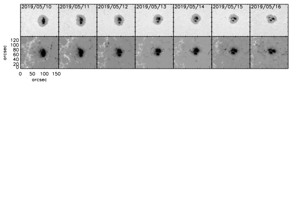
Figure 1: Evolution of NOAA AR 12741 as seen from HMI maps of the continuum intensity (top row) and the vertical component of the magnetic field (bottom row). The maps correspond to 00:00 UT.

3.5 Chromospheric Radiative Loss

The excess radiative loss in the LB over the quiet Sun (QS) was calculated using the procedure described in Rezaei & Beck (2015, their Sect. 4.7) for the MAST Ca II line and the IRIS Mg II k & h lines. Following Neckel & Labs (1984), the intensity of the QS at disk center at the respective central wavelengths was calculated and normalized by the factor arising from the heliocentric angle. The spectra in the QS were then integrated over a 1 Å band around the line core and subtracted from the same in the LB to yield the excess radiative loss.

In order to calculate the total radiative loss in the chromosphere across the full spectrum, we scaled the values obtained from the Ca II 854.2 nm line to the remaining lines in the Ca II IR triplet, the Ca II K & H lines as well as hydrogen Lyman $\alpha$, similar to the procedure described in Rezaei & Beck (2015). The scaling factors were chosen from Yadav et al. (2022, their Table 1) for a region over the polarity inversion line, which is quite similar to the conditions in the LB under study. We assume that the radiative loss in the Ca II IR line at 854.2 nm is a third of the loss of the whole Ca II IR triplet.

For a comparison to the observations we also synthesized the spectral lines of Ca II IR, H & K, Mg II h & k, and Ly$\alpha$ for a characteristic temperature stratification from a location inside the LB and the QS stratification with the Lightweaver code (Osborne & Milić, 2021). Radiative losses for the synthetic spectra were calculated by the same approach as the difference between LB and QS.

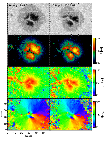
Figure 2: Hinode maps of the leading sunspot in AR 12741 on 2019 May 14 (left) and May 15 (right). Top to bottom: continuum intensity $I_{c}$, field strength $B$, inclination $\gamma$, and azimuth $\phi$. The white rectangle corresponds to the FOV shown in Figure 3.

4 Results

4.1 Evolution of Sunspot in AR 12741

Figure 1 shows the formation and evolution of the LB in the leading sunspot in AR 12741. The leading sunspot appeared on the Eastern limb close to the end of May 6 as a regular, unipolar spot without any conspicuous umbral intrusions. The formation of the LB began in the early part of May 11 with one arm extending from the western section of the umbra-penumbra boundary, eventually reaching the eastern umbral-penumbra boundary in about 8 hr. The onset of convection in the LB was seen in the latter part of May 13, with the subsequent formation of a three-arm structure by May 15, which remained stable until the sunspot traversed the western limb. During this period the sunspot did not fragment or decay into smaller pores/spots and neither were there any significant changes in the global topology of the AR. The vertical component of the magnetic field in the figure shows that the LB stands out in the umbral background with a relatively weaker amplitude. At HMI’s spatial resolution we do not find any indication of opposite polarities in the LB during the lifetime of the sunspot.

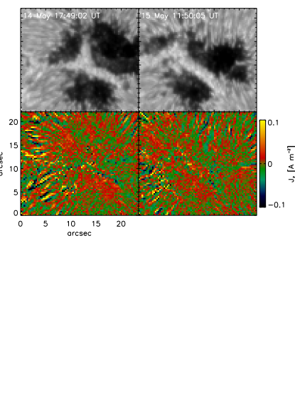
Figure 3: Magnified view of the LB in the SP data in the continuum intensity (top row) and the vertical component of electrical current density (bottom row) for the FOV marked by the white box in Figure 2.

                                                                                 

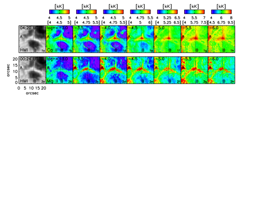
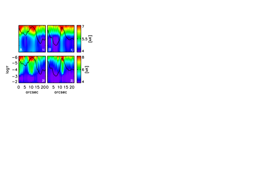
Figure 4: Comparison of temperature stratifications derived from the Ca II and Mg II lines on May 14. Top row, from left to right: HMI continuum intensity (panel a), temperature derived from the MAST Ca II line at different heights from $\log\tau=-3$ to $-6$ (panels b–h), temperature stratification along cut A and cut B in a 2D $x$–$\log\tau$ display (panels i and j). The black lines in panels i and j correspond to the photospheric continuum intensity along cuts A and B, respectively. Bottom row: same as above but for the temperature stratification derived from the IRIS Mg II lines. The temperature maps have been scaled to their respective color bars shown above the panels where the values in parentheses correspond to the Mg II lines.

4.2 Structure of Magnetic Field in LB

Figure 2 shows the Hinode continuum image of the sunspot wherein the LB is seen to comprise bright, small-scale grains in all three arms with an absence of filamentary structures. At most locations, the continuum intensity in the LB is comparable to that in the quiet Sun. The magnetic field is weakest along the axes of the LB, with minimum values ranging between 400 G and 600 G in the three arms. On the other hand, the field strength along the edges of the LB is about 1800–2000 G, while in the umbra it ranges from about 2200 G to 2700 G. The magnetic field inclination increases as one moves from the edge to the axis of the LB with typical values in the interior ranging of about 35^∘–45^∘ in all three arms. As stated earlier, there are no indications of opposite polarities in the LB. The bottom row of Figure 2 reveals that for the most part the azimuth has a smooth radial arrangement in the sunspot, except in the proximity of the LB, which renders three azimuth centers in the respective umbral cores. As the sunspot is of negative polarity, the horizontal magnetic field is predominantly divergent along the LB axis and oriented toward the nearest umbral core.

Figure 3 shows a magnified view of the LB in the continuum intensity and the vertical component of the current density ($J_{z}$). The latter is extremely small in the LB, except at the locations along the axis of the LB, where the horizontal magnetic field appears to diverge into its respective umbral core. These locations are confined to individual pixels where $J_{z}$ can reach up to 0.15–0.25 A m^-2, but these comprise only 3% of the area of the LB. For the majority of the LB, however, the average values of $J_{z}$ are about 0.02 A m^-2 and do not stand out in the same manner as the currents in the penumbra that are relatively stronger by a factor of six. This obvious absence of strong electric currents in the LB is also seen in the Hinode map acquired on May 15. The absence of currents implies that heating by ohmic dissipation cannot be effective.

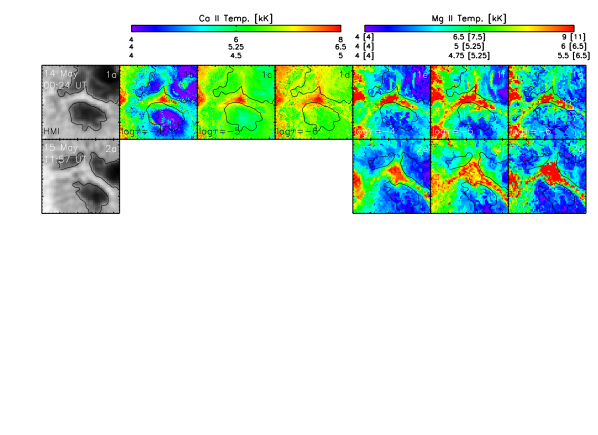
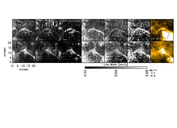
Figure 5: Maps of the temperature, peak intensity, and line width in the LB as a function of height. Top row, from left to right: HMI continuum intensity (panel a), temperature derived from the MAST Ca II line at $\log\tau=-4$, $-5$, $-6$ (panels b–d), and temperature derived from the IRIS Mg II line at $\log\tau=-4$, $-5$, $-6$ (panels e–g). The temperature maps have been scaled to the corresponding color bars above the respective panels, with the numbers from the top to the bottom row below the color bar representing $\log\tau=-6$, $-5$, and $-4$, respectively. The temperature color bar for the IRIS Mg II line is similar, with the numbers in the parentheses corresponding to the observations on 2019 May 15 at 11:57 UT for the maps in the second row. Second row: the same as above on 2019 May 15 at 11:57 UT. Third row: maximum line intensity from the IRIS Mg II line, C II line, Si IV line (panels h–j), line width from the IRIS Mg II line, C II line, Si IV line (panels k–m), and AIA intensity at 171 Å(panel n) on 2019 May 14. Bottom row: the same as above on 2019 May 15 at 11:57 UT. The black contours correspond to the HMI continuum intensity and outline the LB.

4.3 Enhanced, Persistent Brightness over LB

Figure 4 shows the temperature maps of the LB as a function of height as derived from the spectral inversions of the MAST Ca II and IRIS Mg II lines on May 14. The enhanced temperature in the LB appears over an extended height range of $-6.0<\log\tau<-3.5$ with the central junction of the LB being the hottest location. The average temperature at the central junction of the LB is 4960 K, 6430 K, and 7940 K at $\log\tau=-4$, $-5$, and $-6$, respectively, as estimated from the Ca II line. These values in the LB exceed that of the umbra by 840 K, 1165 K, and 1315 K at the above heights, respectively. The temperature maps from the Mg II line exhibit similar values at $\log\tau=-4$ and $-5$ while at $\log\tau=-6$ the temperature is enhanced to 8300 K. The 2D vertical cuts across the LB (panels i and j) show that the thermal enhancement in the LB extends down to $\log\tau=-2$ in the Ca II line while in the Mg II line it is relatively higher at around $\log\tau=-3.5$. The temperature enhancement in the LB arises due to the reduced/suppressed absorption in the Ca II line with the line core intensity being only 20% smaller than the line wing intensity at about 1 Å  (Figure 16 in the Appendix). On the other hand, the Mg II k & h lines comprise strong, compact emission features where the central reversals k3 and h3 are nearly as high as the k2 and h2 emissions.

            

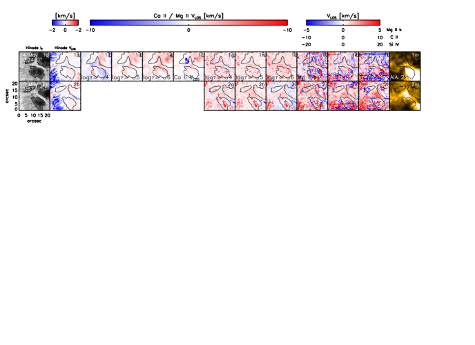
Figure 6: Maps of LOS velocity in the LB as a function of height. Top row, from left to right: Hinode continuum intensity (panel a), Hinode LOS velocity (panel b), LOS velocity derived from the MAST Ca II line at $\log\tau=-4$, $-5$, $-6$ (panels c–e), MAST Ca II Dopplergram (panel f), LOS velocity derived from the IRIS Mg II line at $\log\tau=-4$, $-5$, $-6$ (panels g–i), Doppler shift from the IRIS Mg II line, C II line, Si IV line (panels j–l) and AIA intensity at 171Å(panel m) on 2019 May 14. The velocity maps have been scaled to the corresponding color bars above the respective panels. The black contours, which outline the LB, correspond to the Hinode continuum intensity. Bottom row: the same on 2019 May 15.

                                             

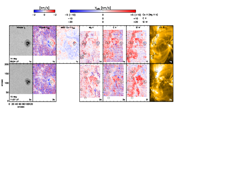
Figure 7: Maps of LOS velocity in AR 12741 as a function of height. From left to right: Hinode continuum intensity (panel a), Hinode LOS Velocity (panel b), MAST Ca II Dopplergram (panel c), Doppler shift from the IRIS Mg II line, C II line, Si IV line (panels d–f) and AIA intensity at 171Å(panel g). The velocity maps have been scaled to the corresponding color bars above the respective panels. The black contours, which outline the LB, correspond to the Hinode continuum intensity. The black squares in panels 1g and 2g indicate the possible location of the outer footpoints of coronal loops that connect to the surroundings of the LB.

   

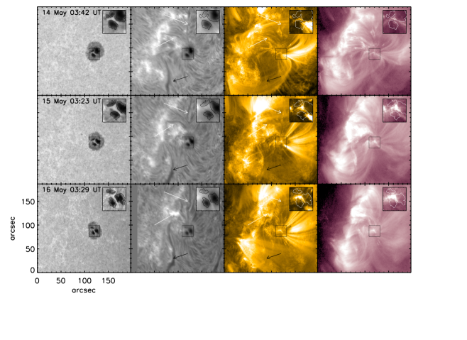
Figure 8: Photospheric, chromospheric, transition region, and coronal morphology in and around AR 12741 from 2019 May 14–16. From left to right: G-band, H-$\alpha$ images from MAST, AIA images in the 171 Å, and 211 Å  channels. The white and black arrows represent arch-filament systems and the AR filament, respectively.

Figure 5 shows the temperature maps from the IRIS Mg II line on May 14 and 15 along with the peak intensity and line width of the C II and Si IV lines in the LB FOV. The temperature enhancement over the LB persists over 36 hr and coincides with the underlying photospheric morphology. A similar characteristic is seen in the peak intensity of the IRIS Si IV line while in the C II line the LB is more diffused on May 14 than it is on May 15. The intensity in the LB is about 80% of the emission in the opposite polarity network flux region as seen in the Mg II and Si IV lines while in the C II it is about 24% and 53% on May 14 and May 15, respectively. The peak intensity of the Si IV line in particular also exhibits structures in the proximity of the LB that are associated with loops rooted at/close to the LB (Figure 17 in the Appendix). The line widths estimated from the single Gaussian fit to the IRIS lines clearly trace the structure of the LB with values of 50 km s^-1, 25 km s^-1, and 30 km s^-1 in the Mg II, C II, and Si IV lines, respectively, on May 14. These values nearly remain the same on May 15 for the Mg II line while there is a marginal increase of about 5 km s^-1 for the C II and Si IV lines. The enhanced, persistent brightness in the LB can also be seen in the AIA 171 Å  and 211 Å  images, which reflect conditions at transition region and coronal temperatures. The enhanced intensity and line widths of the IRIS lines is also observed the following day on May 16, at 03:00 UT. The photospheric LB morphology can thus be traced up to the transition region and corona.

4.4 Velocities with Height in LB

Figure 6 shows the velocity in the LB in the photosphere, chromosphere, and transition region. At the photosphere, the granular LB does not exhibit any strong red- or blueshifts with velocity values ranging between $\pm 0.35$ km s^-1. The velocities in the penumbra, however, are much stronger with the Evershed flow reaching 2 km s^-1. The chromospheric velocities obtained from the inversion of the MAST Ca II and IRIS Mg II k & h lines show that the LB is weakly redshifted by a few km s^-1 which nearly remains the same at heights of $\log\tau<-5$. The velocities obtained from the Gaussian fits to the IRIS lines (panels j–l) reveal that the LB is predominantly redshifted with values of 0.5 km s^-1, 2 km s^-1, and 10 km s^-1 in the Mg II, C II, and Si IV lines, respectively, on May 14. The Mg II line was fitted with a double Gaussian while the C II, and Si IV lines were fitted with a single Gaussian. While these redshifts in the IRIS lines persist in the LB on May 15, the values are increased to 1.5 km s^-1, 5 km s^-1, and 15 km s^-1, respectively. The umbra in particular exhibits the saw-tooth pattern typically associated with shocks as seen in the Mg II and C II lines.

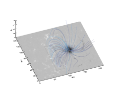
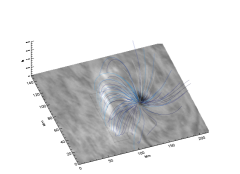
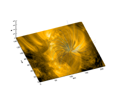
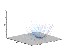
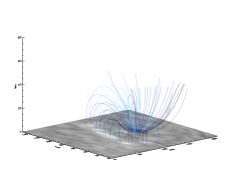
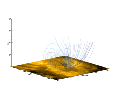
Figure 9: Global magnetic topology of NOAA AR 12741 from a NFFF extrapolation method using the HMI vector magnetic field on May 14 at 04:24 UT. The bottom boundary from left to right corresponds to the vertical component of the magnetic field from HMI, the GONG H-$\alpha$ filtergram, and an AIA 171Å, image, respectively. The black dotted rectangle encloses magnetic field lines from the sunspot that connect to the network region of opposite polarity.

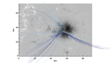
Figure 10: Magnified view of magnetic topology around the sunspot LB.

While the single Gaussian fits to the IRIS lines only show weak redshifts in the LB, an inspection of the spectra emanating from the region in and around the LB reveal supersonic redshifts of about 150 km s^-1 at the extended structure just south of the LB or next to it on May 14. These strong redshifts are associated with the large-scale loops ending in the sunspot (panels 7B–7E of Figure 17 in the Appendix). These spectra have been fitted with a double Gaussian to all the lines, which are also shown in Figure 17. The high-speed downflows are primarily observed in the Si IV line and to very small extent in the C II line (panel 4C). However, the downflows do not appear to persist in time and are greatly reduced as evident in the raster scans on May 14 at 13:21 UT as well as on May 15 at 11:57 UT. Figure 17 also shows the enhanced line width over the LB in all the IRIS lines, which remains a characteristic feature over the course of 36 hr.

Figure 7 shows the spatial distribution of velocities over the FOV of the AR. As stated earlier, the strongest velocities in the sunspot at the photosphere are associated with the Evershed flow, while in the chromosphere the inverse Evershed flow is observed in the superpenumbral region with values of about 2 km s^-1 and $-1.3$ km s^-1 in the center-side and limb-side regions, respectively (panel 1c). In the IRIS C II and Si IV the FOV is dominated by redshifts particularly in the network flux region and the arch-filament systems around the leading sunspot with values in the Si IV being the strongest and reaching about 20 km s^-1. On the other hand, blueshifts appear sporadically in patches across the arch-filament systems as well as in the large filament east of the sunspot that extends southward, where the velocities are about $-3$ km s^-1 and $-10$ km s^-1, respectively, as estimated from the Mg II line (panel 2d).

We also visually identified the footpoints of the AIA 171 Å loops that begin from the LB and the sunspot and possibly end in the opposite polarity network flux region (squares in the panel).

The majority of the footpoints are dominated by redshifts or extremely weak blueshifts apart from square A in panel 1d with a blueshift of about $-5$ km s^-1. The transition region lines C II and Si IV show dominantly redshifts all the time. The same trend is seen in the velocity maps on May 15. However, unlike on May 14, the visible loops that begin at or close to LB do not appear to terminate at the opposite polarity network flux region.

   

   

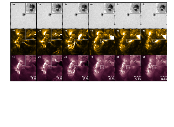
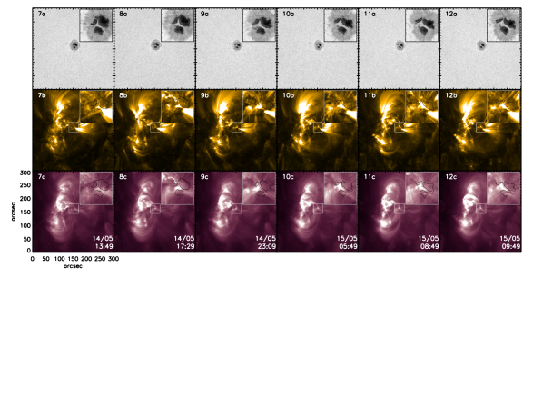
Figure 11: Evolution of the LB as seen in the transition region and corona. The top, middle, and bottom panels correspond to the HMI continuum intensity and AIA 171Å  and 211Å channels, respectively. The small white square in the middle of the FOV represents the LB whose magnified image is shown in the inset in the top right corner of the panel. The larger AIA images are clipped between 20 and 1500 counts in both AIA channels. The insets on the other hand are scaled between 100–900 and 100–1000 counts in the 171 and 211Å channels, respectively.

4.5 Global Topology and Morphology of AR

We now discuss the large-scale structures in the chromosphere, transition region, and corona in the context of the temporal stability of the LB. Figure 8 shows that there are several, small arch-filament systems north of the leading sunspot that connect to the following polarity. In addition, a large filament located east of the sunspot extends southward beyond the MAST H$\alpha$ FOV and arches around to the west back toward the AR. These arch-filaments systems as well as the large AR filament also remain stable over a period of 36 hr. The figure also shows that while the LB remains persistently bright in the AIA 171 Å  and 211 Å images, there are large-scale loops that are always rooted at one end of the LB or close to it, which is seen from May 14 to May 16. In addition, these large-scale loops extend over and above the AR filament as observed on May 14.

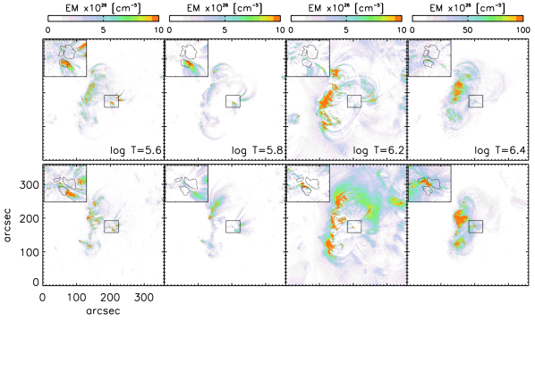
Figure 12: Emission Measure estimated from the AIA images using the 171, 211, 193, 335, 131, 94 Å channels at different temperatures. The top and bottom panels correspond to 2019 May 14 May at 00:24 UT and 2019 May 15 at 11:57 UT. The magnified view of the light bridge is shown in the inset in the top left corner. The thin black contours correspond to the HMI continuum intensity.

The global topology of the AR is further demonstrated from the extrapolation of the photospheric magnetic field using the NFFF technique as shown in Figure9 on May 14. The sunspot magnetic field is consistent with a simple bipolar structure without any discernible signatures of twist. Field lines from the eastern penumbral region of the sunspot connect to the opposite polarity network flux region (black dotted rectangle in the figure) while those from the umbra and the western part of the sunspot comprise open field lines. The average height of the closed field lines connecting the sunspot to the following polarity is about 12.3 Mm, while field lines starting from the inner penumbra can reach heights of up to 30 Mm. An estimation of the loop height was independently made when the sunspot was very close to the western limb on May 19. An unsharp masked AIA 193 Å  image provided a side view of the loops along the sky plane from which a height of about 13 Mm was estimated (see Figure 18 in the Appendix), which is in good agreement with those calculated from the extrapolated field lines. A zoom-in of the LB FOV (Figure 10) shows the field being nearly vertical at the central part while toward the western end the field lines fan out with height. The LB thus seems to be related to features of the AR magnetic topology that govern its large-scale shape and evolution, at least in the sense of having their apparent footpoints in its vicinity.

Figure 11 shows the temporal evolution of the corona above the AR from May 13 to May 15. On May 13, a B3.5 class flare occurred at 15:02 UT, with the peak at 15:52 UT. The flare involved the eruption of the large AR filament south of the sunspot that was associated with a mass ejection that had a linear speed of 312 km s^-1, a position angle of 234^∘ and was seen in the Large Angle Spectroscopic Coronagraph (LASCO; Brueckner et al., 1995) C2 FOV at 17:48 UT as obtained from the Cactus (Robbrecht et al., 2009) catalog. The erupting filament and the associated coronal dimming can be seen in the lower part of panel 2 of Figure 11. The bright ribbon from the flare stretches all along the LB and stands out from the rest of the sunspot (panels 2b and 2c of Figure 11). Similarly, the post flare loops from the ensuing eruption are rooted along the extended network flux region in the following group of sunspots of the AR while the other end is more confined and located at the eastern end of the LB (panel 3 of Figure 11). There were no flares in the AR on May 14; however small-scale coronal activity was observed over the LB later in the day at around 17:30 UT (panel 8). There were four flares on May 15, which included a C2.0 class flare and three weak B-class flares. However, none of these flares were eruptive and primarily involved the arch filament close to the northeastern periphery of the sunspot where one of the flares ribbons was seen. The other set of ribbons were located in the opposite polarity network flux region.

The AIA images clearly show the enhanced intensity over the LB as well as the presence of loops at or close to it, both of which persist over a duration of 3 days. Especially in panels 8–12 of Figure 11, both AIA channels at 171Å  and 211Å  closely mimic the photospheric shape of the LB but at transition region heights.

4.6 Energy Budget from Various Mechanisms

In this section we compare the energetics from various mechanisms/processes that could contribute to the sustained heating over the LB for a duration of the observations.

(i) Thermal energy in the EUV: The thermal energy emanating in the LB at EUV wavelengths can be estimated as

$$E_{th}=3n_{e}k_{b}Tl^{3},$$ (1)

where $n_{e}$, $k_{b}$, $T$, and $l$ are the electron density, Boltzmann constant, temperature, and length scale over which the brightening in the LB is observed, respectively. To ascertain the temperature in the LB, we calculate the Differential Emission Measure (Cheung et al., 2015) from the various AIA channels, namely, 171, 211, 193, 335, 131, 94 Å. Figure 12 shows the emission measure (EM) at various temperatures, where the LB clearly stands out between $6.2\leq\log{T}\leq 6.4$. The electron density $n_{e}$ can then be estimated as $n_{e}\approx\sqrt{EM/l}$. The value of the length scale $l$ is estimated from the volume, using the area of the LB (25.8 Mm² and 35.7 Mm² on May 14 and 15, respectively) and a vertical height of 4 Mm. The electron density $n_{e}$ was computed using the mean DEM over the LB area and averaged over a temperature range of $\log T=6.2$ to $6.4$. With $T=2.5$ MK, and $n_{e}=1.8\times 10^{9}$ cm^-3 ($2.5\times 10^{9}$ cm^-3), we obtain $E_{th}=1.9\times 10^{26}$ ($3.7\times 10^{26}$ erg) in the LB on May 14 (15).

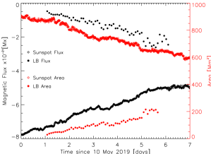
Figure 13: Temporal evolution of the magnetic flux and area of the sunspot and light bridge. The y-axes on the left and right correspond to the flux and area, respectively. The light bridge flux and area have been enhanced by a factor 5 for better visibility.

(ii) Thermal Energy in the Visible and NUV: The enhancement in internal energy can be computed from the temperature stratification derived from the inversion of the MAST Ca II and IRIS Mg II lines following Beck et al. (2013b).

$$\Delta E_{int}=\frac{R}{\mu(\gamma-1)}\Delta A\sum_{i=z0}^{z1}\rho_{i}\Delta z_{i}\sum_{j,k}\left(T^{lb}_{i,j,k}-\overline{T}^{umb}_{i}\right),$$ (2)

where $R=8.31$ J mol^-1 K^-1, $\mu=1.3$ g mol^-1, $\gamma=5/3$, $\rho$ is the gas density, $\Delta A$ is the area of the pixel, $T^{lb}$ is the temperature in the LB, and $\overline{T}^{umb}$ is the average temperature in the umbra. The summation with index $i$ is carried out from $z0$ to $z1$, which are the geometric heights at $\log\tau=-4$ and $\log\tau=-6$, respectively. The values of the geometrical height and gas density $\rho_{i}$ at different optical depth points were taken from the Harvard Smithsonian Reference Atmosphere (HSRA; Gingerich et al., 1971). Indices $j$ and $k$ correspond to the spatial domain, while $\Delta z_{i}$ is the geometric height spacing between adjacent optical depth points. Equation 2 yields $4.7\times 10^{25}$ erg and $8.6\times 10^{25}$ erg for the thermal energy from the Ca II and Mg II lines, respectively. $E_{th}$ is the enhancement in thermal energy over the surroundings of the LB, not the total energy. As it persists for days in a stationary way and the chromospheric relaxation time is on the order of a few minutes, the excess energy losses that lead to the enhancement must be replenished all the time by a continuing heating process.

(iii) Kinetic energy associated with LB expansion: Figure 13 shows the temporal evolution of the sunspot flux and area, both of which decrease nearly linearly with time. The area of the LB on the other hand shows an increase with time, with a linear fit yielding a value of 5.7 Mm²day^-1. Using the width of the LB of 3.3 Mm on May 15, we can associate the linear expansion speed ($v_{frag}$) of the LB to the kinetic energy as

$$E_{kin}=0.5Ad\rho v_{frag}^{2},$$ (3)

where $\rho$ is the photospheric density, $A$ is the area of the LB, and $d$ is the depth to which the convective structure extends to, which we assume to be 6 Mm (Rempel et al., 2009). Using the above area increase and width of the LB, we obtain a value of 20 m s^-1 for $v_{frag}$. We express the area and the density as a function of depth, namely, $\rho(z)=\rho_{s}\exp{(z/\tau_{\rho})}$ and $A(z)=A_{s}\exp{(-z/\tau_{B})}$, where the suffix $s$ stands for the surface/photosphere and the scale heights in the two expressions correspond to the density and magnetic field. The values for $\tau_{\rho}$ and $\tau_{B}$ are 0.5 Mm and 2 Mm, respectively, while $\rho_{s}$ and $A_{s}$ are $10^{-7}$ g cm^-3 and 35.7 Mm², respectively. The kinetic energy can then be expressed as

$$E_{kin}=\int_{0}^{d}0.5A(z)\rho(z)v_{frag}^{2}dz,$$ (4)

Using the above values, we obtain $E_{kin}=3.9\times 10^{28}$ erg. For comparison, the convective energy of solar granulation with an rms velocity of 0.5 km s^-1 (Beck et al., 2009, 2013a) over the same area as the LB and using Eqn. 4, is about $2.4\times 10^{31}$ erg, which is nearly 3 orders of magnitude larger than the one from the expansion in the LB.

Table 2: Summary of energy estimates from different mechanisms for May 14 and May 15.

Mechanism	Energy (erg)
	May 14	May 15
Thermal Energy in EUV	$1.9\times 10^{26}$	$3.7\times 10^{26}$
Thermal Energy in UV &	$8.6\times 10^{25}$	–
Visible	$4.7\times 10^{25}$	–
Total Thermal Energy	$3.2\times 10^{26}$	–
Total Chromospheric	$3\times 10^{26}$
Radiative Loss
Kinetic Energy	$3.9\times 10^{28}$	–
Magnetic Flux	$7.5\times 10^{27}$ [S]	–
	$2.1\times 10^{26}$ [LB]
Freefall	$6.3\times 10^{26}$	$8.7\times 10^{26}$

(iv) Energy related to magnetic flux loss/gain: As seen earlier, the sunspot loses magnetic flux at a rate of $\phi_{t}=1.8\times 10^{19}$ Mx hr^-1, which was derived from a linear fit to the flux curve in Figure 13. Similarly, the rate of flux increase in the LB is about $3.1\times 10^{18}$ Mx hr^-1. The magnetic flux in the LB increases because its area increases and the HMI data show a non-zero magnetic flux at those places. The energy related to the loss of flux can be expressed as

$$E_{flux}=\frac{1}{8\pi}\frac{(\phi_{t}t)^{2}}{h},$$ (5)

where $t$ is the time scale over which the flux lost/gained can supply the energy ($\sim$10 min) and $h$ is the chromospheric heating height scale ($\sim$500 km; Chitta et al., 2018). The loss of flux in the sunspot provides an energy of $7.5\times 10^{27}$ erg, while that gained in the LB is about $2.1\times 10^{26}$ erg.

(v) Free fall energy: The free fall energy of plasma draining down a loop from a height $h$ in the corona can be expressed as

$$E_{fall}=\rho Ag_{\odot}h^{2},$$ (6)

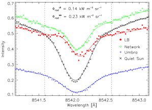
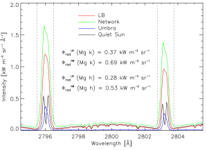
Figure 14: Top panel: MAST Ca II spectra from different locations in the FOV. The symbols and the solid lines correspond to the observed and synthetic profiles, respectively. Bottom panel: observed IRIS Mg II k & h lines for the same locations. The dashed vertical lines mark the wavelength region within which the excess radiative losses were calculated. Their values for the network (NW) and the LB are given inside the panels.

where $A$ is the area of the LB, and $\rho$ is the coronal gas density. The loop height $h$ as derived from the extrapolations is about 12.3 Mm. Using values of $\rho$ of $5\times 10^{-11}$ kg m^-3, $g_{\odot}$ as 273.7 m s^-2 and $A$ of 25.8 Mm² and 35.7 Mm² on May 14 and 15, respectively, $E_{fall}$ is estimated to be about $6.3\times 10^{26}$ erg and $8.7\times 10^{26}$ erg on May 14 and 15, respectively;

The energy estimates from the different physical mechanisms that could be the sources are summarized in Table 2.

4.7 Estimates of Radiative Losses

The top panel of Figure 14 shows Ca II spectra and their synthetic fits from different regions in the FOV, i.e., the umbra, LB, QS, and magnetic network. The excess radiative loss in the LB with respect to the QS is about 0.14 kW m^-2 ster^-1 as derived from the calculation described in Sect. 3.5. In comparison, the excess loss in the network region is about 1.6 times higher at 0.23 kW m^-2 ster^-1. The excess radiative losses in the LB over the QS as estimated from the Mg II k & h lines are 0.37 kW m^-2 ster^-1 and 0.28 kW m^-2 ster^-1, respectively (bottom panel of Figure 14). The spectral synthesis of the LB and QS temperature stratifications yields excess radiative losses in the LB that are a factor of 2–3 smaller than for the observations (second row in Table 3) with, e.g., 0.1 kW m^-2 ster^-1 for Mg II h and 0.09 kW m^-2 ster^-1 for Ca II IR at 854 nm. The difference to the observations is presumably caused by the assumed density stratification in the synthesis and the lack of 3D radiative transfer. The direct observations can be taken to be more accurate in this context.

Table 3: Estimates of radiative losses in different phenomena in excess of the QS. Ca II IR refers to the spectral line at 854.2 nm.

No.	Type	$\Theta$ (∘)	Reference	Excess Radiative Loss $\Phi_{rad}$ (kW m-2 ster-1)
				Mg II k	Mg II h	Ca II K	Ca II H	Ca II IR	L$\alpha$	H$\alpha$
1.	Sustained Heating in LB	17	Current Study	0.37${}^{\textrm{\tiny{O}}}$	0.28${}^{\textrm{\tiny{O}}}$	0.27${}^{\textrm{\tiny{S}}}$	0.19${}^{\textrm{\tiny{S}}}$	0.14${}^{\textrm{\tiny{O}}}$	0.03${}^{\textrm{\tiny{S}}}$
	Spectral Synthesis in LB			0.1	0.08	0.1	0.1	0.09	0.01
2.	Polarity Inversion Line	52	Yadav et al. (2022)	0.28	0.25	0.6	0.43	0.31	0.07
3.	Ohmic Dissipation in LB	13	Louis et al. (2021)					0.35
4.	Flare Ribbon	52	Yadav et al. (2022)	2.23	1.98	1.76	1.34	0.78	0.57
5.	Flare Ribbon	29	IBIS DST 2014/10/24					0.89		2.17
6.	Ellerman Bomb	70	Rezaei & Beck (2015)				11	1.5		4

^O: derived from observations ^S: derived from scaling factors from the second row

The factors for the radiative loss in the LB over the QS for the Ca II K & H lines and Ly$\alpha$ are 0.65, 0.46, and 0.08 times the Ca II IR triplet (3$\times$Ca II IR at 854 nm), respectively, using the values from the third row of Table 3. Adding the contributions from all the spectral lines in the first row of Table 3 and integrating over the solid angle of $4\pi$, the total chromospheric radiative loss in the LB is about 19.7 kW m^-2 in excess of the QS. In terms of energy the above value translates into 3$\times$10²⁶ erg using the LB area of 25.8 Mm² and a time scale of 1 min, where the latter takes the chromospheric relaxation time (Beck et al., 2008) into account, given that the heating in the LB is persistent over days and thus needs to be replenished continuously. For comparison, the total thermal energy in the EUV (1.9$\times$10²⁶ erg), UV (8.6$\times$10²⁵ erg), and visible (4.7$\times$10²⁵ erg) on May 14 (refer Table 2), is about 3.2$\times$10²⁶ erg together, which gives a close match to the energy in the radiative losses that are a sink of energy.

Figure 15 shows representative spectra of the Ca II 854.2 nm line from a few other phenomena such as an Ellerman bomb (EB), a flare ribbon, and a case of ohmic heating in an LB for comparison, whose radiative losses are also listed in Table 3. The radiative loss in an EB is about 1.5 kW m^-2 ster^-1 (Rezaei & Beck, 2015), while that of a flare ribbon is about 0.89 kW m^-2 ster^-1. Similarly, ohmic dissipation in an LB comprises about 0.35 kW m^-2 ster^-1 (Louis et al., 2021), which is about 2.5 times greater than the value obtained for the LB under investigation. The current case of continuous long-term heating is thus at the lower end of the energy range of more short-lived and dynamic events.

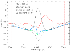
Figure 15: Illustrative spectra of different phenomena (solid lines). The black dashed line represents the QS profile. The vertical red dotted lines at $\pm 2$ Å  are the wavelength regions within which the radiative loss for the EB was calculated, while the vertical black dotted lines correspond to the range used for the flare ribbon and ohmic dissipation.

5 Discussion

5.1 LB Properties and Evolution

The granular LB that formed in a regular, unipolar sunspot remained stable until the AR traversed the solar limb. During this time, the host sunspot did not fragment nor were there any large-scale changes in the magnetic structure of the AR. Measurable changes were seen in the flux of the sunspot and the area of the LB, which decreased and increased by $1.7\times 10^{21}$ Mx and 22 Mm², respectively, over the course of four days. While overturning convection is prevalent in the LB at photospheric heights, the LB is heated over a large temperature range from 8000 K to 2.5 MK spanning the chromosphere to the low corona that is sustained for more than two days. The signatures of this heating are seen in the temperature maps of the chromospheric Ca II and Mg II spectral lines, the peak amplitude and line width of the IRIS C II, Si IV lines that form at a temperature of 30,000 K and 65,000 K, respectively, and the emission measure using the different AIA channels. The enhanced intensities and line widths of the IRIS lines in the LB are in good agreement with Rezaei (2018). The persistent heating over the LB is counterintuitive as the underlying structure would radiate the majority, if not all, of its energy once having evolved to a strongly convective region inside the sunspot. We now discuss the possible mechanisms that can provide the necessary energy to sustain the enhanced temperature over the LB for more than two days.

5.2 LB Energy Budget

Thermal Energy and Radiative Losses

An estimate of the thermal energy in the visible, NUV, and EUV yields about $3.2\times 10^{26}$ erg using the values on May 14 as shown in Table 2. The chromospheric temperature in the LB is enhanced compared to its immediate umbral surroundings and even with respect to QS conditions. The enhanced temperature persists over a few days in a similar way. The heating process has thus lifted the temperature to a new, higher energetic equilibrium that is maintained in time.

The estimate of the chromospheric instantaneous excess energy losses over the LB area yields $3\times 10^{26}$ erg, which gives a close match to the predicted losses from the temperature excess. This confirms the presence of a new stationary equilibrium at a higher energy level than, e.g, in the QS. In comparison to typical values for other chromospheric heating events such as ohmic dissipation (Louis et al., 2021), flare ribbons (Yadav et al., 2022) or an Ellerman bomb (Rezaei & Beck, 2015) the current radiative losses are found to be at the low end of the range. Apart from ohmic dissipation, the other types of heating events are generally impulsive and short-lived with time scales of only a few tens of minutes with spatially localized heating sources from reconnection (Georgoulis et al., 2002) or particle beams (Kleint et al., 2016). While flare ribbons can cover similar areas as the current LB, the heating process that causes its enhancement must be both spatially extended and long-lived, albeit at a 6–10 times lower heating rate than for the more impulsive events.

LB Expansion and Freefall Acceleration

The kinetic energy associated with the LB expansion is 1–2 orders of magnitude higher than the net thermal energy. This mechanism is related to photospheric dynamics that can lead to the buildup of energy in the corona. Mackay et al. (2011) showed that photospheric footpoint motions in a decaying AR could store enough free magnetic energy in the corona to compensate the radiative losses. Using idealized numerical models, Hurlburt et al. (2002) showed that by directly coupling compressible magneto-convection at the bottom layer to a low plasma-$\beta$ region above, the overlying corona could be heated by the Poynting flux emerging from the upper boundary. The LB expansion continues on the same temporal and spatial scales as the heating process over days. The heating seems to be localized above the LB area also in the higher atmosphere, which indicates a correlation to the photospheric spatial pattern. It is unclear, however, how the photospheric mechanical energy would be transported upward and deposited locally in the chromosphere and transition region in the current case.

Freefall acceleration of plasma along loops (Schad et al., 2021) connecting the opposite polarity network flux to the LB or close to it in the sunspot could also provide sufficient energy to sustain the temperature over the LB. The long-lived presence of loops at or near the LB and the persistent brightness in the AIA channels suggest that this could also be a likely possibility. However, with the exception of a few locations in the umbra next to the LB we do not see any strong redshifts in the C II or Si II lines that would indicate plasma draining down the loop from a height of 12 Mm. Coronal rain was also found to be often rather intermittent in nature without continuous flows (Antolin et al., 2012; Li et al., 2021).

Furthermore, we do not unambiguously detect blueshifts at the other end of the loops, which would provide evidence for a siphon flow (Cargill & Priest, 1980; Straus et al., 2015; Prasad et al., 2022). The LB along with the network flux region are redshifted, which raises questions on how any flow would be sustained for a period of days. While the Doppler shift measurements in the LB do not reveal high-speed downflows all the time, the enhanced intensity as well as line width are maintained in the LB for over two days.

Magnetic Flux Losses and Field-related Heating

The energy corresponding to the magnetic flux loss of the sunspot or the apparent gain of magnetic flux above the LB does also match the energy requirements from the radiative losses and the thermal energy. They occur continuously on the same time scale as the persistent LB heating. The total loss of magnetic flux of the sunspot would, however, not match the required localized heating with a preferred occurrence above the LB area, while the apparent gain of magnetic flux above the LB area would require a nearly complete conversion of magnetic to thermal energy to balance the radiative losses. Harra & Abramenko (2012) showed that magnetic flux dispersal at the photosphere is important for the release of nonthermal energy in the corona for a decaying AR that was devoid of flux emergence. The photospheric interactions of a bipole containing a flux of $2\times 10^{18}$ Mx with an overlying field via cancellation, emergence, and relative photospheric motions could dissipate about $1.3$–$3.2\times 10^{26}$ erg in the corona over a time interval of 100 minutes (Meyer et al., 2012). Using the magnetofrictional approach of Yang et al. (1986), Meyer et al. (2013) evolved the corona through a sequence of nonpotential, quasi-static equilibria using photospheric LOS magnetograms at the bottom boundary. They found that the storage of energy and its subsequent dissipation in the quiet corona occurred at a mean rate of $8.7\times 10^{4}$ erg cm^-2 s^-1, and produced dark and bright features similar to those in EUV images. The so-called braiding of magnetic flux by random photospheric motions (Parker, 1972; Peter et al., 2004) could set in at the boundary layer between the presumably field-free overturning convection in the LB and the surrounding umbral magnetic fields. For the case of the current LB, the resulting heating would, however, have to set in very low in the atmosphere starting at chromospheric levels.

Wave Heating

As the LB exhibits convective motions that are possibly rooted quite deep, magneto-acoustic waves could dissipate a part of their energy in the higher atmospheric layers (Ulmschneider et al., 1978; Kalkofen, 2007; Khomenko & Cally, 2012; Kayshap et al., 2018). The acoustic energy flux estimated from a number of chromospheric lines shows that at least in the quiet Sun, it is able to balance the radiative losses at heights between 900 and 2200 km (Abbasvand et al., 2020a, b). However, in active regions the acoustic flux balances only 10–30% of the radiative losses (Abbasvand et al., 2021). This is also in agreement with previous studies by Beck et al. (2009). Based on the above, and coupled with the lack of time series IRIS observations with high temporal cadence, one can argue that the residual acoustic flux would only have a minor, if not negligible, contribution in heating the LB to transition region and coronal temperatures. On the other hand, Alfvén waves have been proposed as possible energy transporters that could heat the upper atmospheric layers (Osterbrock, 1961; Stein, 1981; van Ballegooijen et al., 2011; Sakaue & Shibata, 2020) with direct evidence for an energy deposit in the chromosphere in Grant et al. (2018). Thus, we cannot rule out the possibility of Alfvén waves heating the chromosphere and transition region above the LB, with the caveat that the nearly vertical smooth magnetic field would make a mode conversion and subsequent energy deposit difficult.

Ohmic Dissipation

Ohmic dissipation in the LB could arise from electric currents due to the presence of weak magnetic fields inside the sunspot. Recently, Louis et al. (2020) reported the bodily emergence of horizontal magnetic fields along an LB that comprised strong blueshifts all along the LB lasting for a period of 13 hr. The emergence of flux rendered strong electric currents leading to ohmic dissipation that was accompanied by large temperature enhancements in the chromosphere above the LB (Louis et al., 2021). A similar observation of blueshifts and chromospheric emission was seen during the emergence of a small-scale, bipolar loop in a granular LB (Louis et al., 2015). However, the granular LB analyzed here did not comprise any strong or significant velocities in the photosphere, and the photospheric currents were very weak or negligible. For ohmic dissipation to play a role in the chromosphere and above, the currents at the bottom boundary have to be the strongest for them to be significant in the higher layers, which is not the case here.

Transient Chromospheric Events

LBs are known to exhibit a range of transient phenomena, including jets (Louis et al., 2014), brightenings (Louis et al., 2008), and flares (Louis & Thalmann, 2021). There were several confined, however weak, flares originating in the AR on May 15 and an eruptive flare on May 13 which resulted in one of the flare ribbons, although compact, to be co-spatial with the LB. However, there were no flares associated with the LB or the AR on May 14. The spatial coincidence of one of the flare ribbons along the LB and the ensuing post flare loops extending to the LB indicate the connectivity of the LB to the large-scale topology of the AR, which was destabilized by the erupting filament below. The association of an LB with the large-scale topology of an AR has also been observed by Guo et al. (2010), where repetitive surges from an LB led to the eruption of an adjacent filament. While the flares could play an important role in depositing energy in the higher layers of the LB, which would subsequently heat the lower layers, the strength of the flares, and the rapid radiative cooling would not explain the persistent brightness of the LB over 48 hr. In addition, the IRIS SJ images do not indicate any discernible, small-scale, reconnection-driven events during the raster scans, although we do not rule out the possibility that these could have been missed during the data gap. Even if there were small-scale ejections, they would be localized and would not explain the heating over the entire extent of the LB.

The case of sustained heating over a granular LB is not uncommon. Berger & Berdyugina (2003) reported a constant brightness enhancement over a granular LB using the 1600 Å  channel of the Transition Region and Coronal Explorer (TRACE; Handy et al., 1999). A C2.0 flare was also observed wherein one of the ribbons was co-spatial with the LB similar to the observations reported in this study. The authors attributed the persistent brightness to the stressed magnetic configuration at the LB that could lead to reconnection and energy dissipation. As stated above, the lack of electric currents rules out ohmic dissipation as the source(s) of heating over the LB.

5.3 Possible Heating Process(es)

The energy estimates associated with the loss/gain of magnetic flux, increase in the LB area, and freefall acceleration exceed the thermal energy in the LB that matches the radiative losses. However, it remains unclear if one or a combination of the above processes are the primary source of heating over the LB. Only some of the possible processes match the necessary temporal (long duration) and spatial patterns (concentration on LB area). The heating rate is found to be lower than for other impulsive chromospheric heating events. A process related to the photospheric mechanical energy from either the LB expansion or the overturning convection inside the LB and its interaction with bordering magnetic fields seems to be more likely because a continuous driver over days is needed.

As pointed out by Rezaei (2018), LBs are multithermal structures, with diverse heating mechanisms supplying momentum and energy to different layers of the solar atmosphere. It remains an open question whether such a persistent heating over a large height range in a granular LB is indeed a generic phenomenon. In the current study, we could especially not determine whether the energy that heats the LB region at different heights is converted from other energy sources and deposited locally, or results from either an upward or downward energy transfer through the outer solar atmosphere.

6 Conclusions

The LB under investigation evolved sufficiently to exhibit overturning convection without fragmenting the regular, unipolar sunspot. Despite the absence of any large-scale flux emergence or apparent changes in the magnetic topology of the AR, the LB was associated with strong heating spanning a temperature range of 8000 K to 2.5 MK, which was maintained for more than two days. In addition to the persistent brightness, large-scale coronal loops are always rooted at or close to the LB. The estimated thermal energy from the EUV, NUV, and visible spectral regions is about $3.2\times 10^{26}$ erg and lines up with estimates of the chromospheric radiative losses. The continued heating could be accounted for by one, or a combination of the following processes, namely, loss of magnetic flux, kinetic energy from the lateral expansion of the LB or overturning convection inside it, and freefall acceleration of plasma along coronal loops. The absence of strong electric currents in the LB rules out heating by ohmic dissipation. Further studies are needed to determine if such sustained heating is a general characteristic of sunspot LBs or whether the LB in this study is a rare exception.

Appendix A MAST Ca II and IRIS Mg II Spectra

Figure 16 shows the observed and synthetic spectra in the MAST Ca II and IRIS Mg II lines along with their temperature stratifications for a few spatial locations in the FOV. The synthetic spectra from the NICOLE and IRIS² inversions match the observed spectra quite well with the resulting temperature stratification having a nearly smooth variation in the spatial and height domain. While the Ca II and Mg II lines both show an enhancement in temperature over the LB at heights above $\log\tau=-3$, the spectral signatures in the two lines are quite distinct.

At the highest layers near $\log\tau=-6$, the temperature in the LB is nearly comparable to that in the opposite polarity network flux region being cooler than the latter by about 100 K  as estimated from the Ca II line. In comparison, the temperature difference is about 800 K  in the Mg II. However, the stratification in the lower heights is very similar between the LB and the network region as seen in both lines.

                       

                       

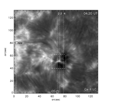
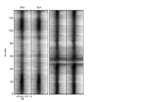
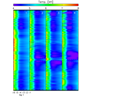
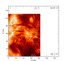
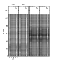
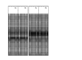
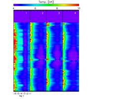
Figure 16: Top panels: NICOLE inversion results in the LB from MAST observations of the Ca II line at 854.2 nm. The dashed white square indicates a smaller FOV around the LB, which is depicted in Figure 4. The locations marked ‘NW’ and ‘QS’ correspond to the network and quiet Sun, respectively, and whose profiles are shown in Figure 14. The middle panels show the observed and synthetic spectra for the four vertical cuts in the line core image. The right panels correspond to the temperature stratification along the four cuts. The white horizontal dashed lines in the middle and right panels depict the spectral region corresponding to the LB and the associated temperature stratification, respectively. Bottom panels: Same as above but for the IRIS Mg II line.

Appendix B IRIS NUV and FUV lines

Figure 17 shows the peak intensity and spectra in the IRIS NUV and FUV lines in the LB at different instances of time spanning a duration of 36 hr. The panels to the right of the LB FOV correspond to the observed and fitted spectra with the latter being derived from a double Gaussian fit and indexed with an $\ast$. All three IRIS lines show the LB to have a pronounced line width although this is less conspicuous for the C II on May 14. While the Mg II and C II lines show the LB with an enhanced intensity, the Si IV lines show additional structures that are possibly related to the coronal loops ending in the sunspot and are often seen very close to the LB. These secondary structures sometimes show redshifts in excess of 100 km s^-1  which are reproduced very well in the double Gaussian fit.

                       

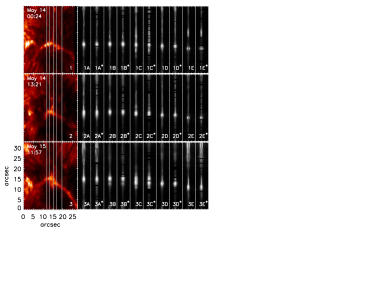
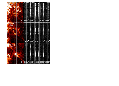
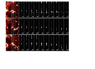
Figure 17: Spectral profiles of IRIS lines and their corresponding fits. Panels 1, 4, and 7 correspond to the maximum intensity of the Mg II k line, the C II line, and Si IV line, respectively. The vertical lines represent cuts whose spectra are shown on the right of each panel indexed A–E, while the corresponding fits are indicated with an $\ast$. The fits to spectra were obtained using a double Gaussian profile.

Appendix C Loop Height Estimate from AIA Images

                              

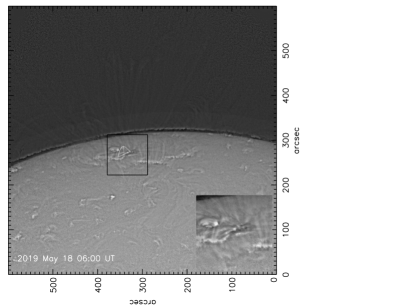
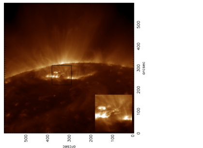
Figure 18: Left: Composite of contrast enhanced AIA 193 Å  channel image and an HMI continuum intensity image with the white line tracing the loop starting from the LB. The inset on the lower right shows the magnified view of the loop extending down to the LB. Right: AIA 193 Å image for the same FOV as the left panel. The images have been rotated for a better viewing perspective.

Figure 18 shows the presence of coronal loops over AR 12741 when the spot was very close to the western limb. Using an unsharp image from the AIA 193 Å  channel, we manually detect loops connecting the spot to the following polarity that appear as the extended network flux to the east and southeast of the AR. The trace along one such set of loops along with the height is shown in the left panel of the figure.

References

- Abbasvand et al. (2020a) Abbasvand, V., Sobotka, M., Heinzel, P., et al. 2020a, ApJ, 890, 22, doi: 10.3847/1538-4357/ab665f
- Abbasvand et al. (2021) Abbasvand, V., Sobotka, M., Švanda, M., et al. 2021, A&A, 648, A28, doi: 10.1051/0004-6361/202140344
- Abbasvand et al. (2020b) —. 2020b, A&A, 642, A52, doi: 10.1051/0004-6361/202038559
- Antolin et al. (2012) Antolin, P., Vissers, G., & Rouppe van der Voort, L. 2012, Sol. Phys., 280, 457, doi: 10.1007/s11207-012-9979-7
- Asai et al. (2001) Asai, A., Ishii, T. T., & Kurokawa, H. 2001, ApJ, 555, L65, doi: 10.1086/321738
- Beck et al. (2013a) Beck, C., Fabbian, D., Moreno-Insertis, F., Puschmann, K. G., & Rezaei, R. 2013a, A&A, 557, A109, doi: 10.1051/0004-6361/201321596
- Beck et al. (2009) Beck, C., Khomenko, E., Rezaei, R., & Collados, M. 2009, A&A, 507, 453, doi: 10.1051/0004-6361/200911851
- Beck et al. (2013b) Beck, C., Rezaei, R., & Puschmann, K. G. 2013b, A&A, 553, A73, doi: 10.1051/0004-6361/201220463
- Beck et al. (2008) Beck, C., Schmidt, W., Rezaei, R., & Rammacher, W. 2008, A&A, 479, 213, doi: 10.1051/0004-6361:20078410
- Berger & Berdyugina (2003) Berger, T. E., & Berdyugina, S. V. 2003, ApJ, 589, L117, doi: 10.1086/376494
- Brueckner et al. (1995) Brueckner, G. E., Howard, R. A., Koomen, M. J., et al. 1995, Sol. Phys., 162, 357, doi: 10.1007/BF00733434
- Cargill & Priest (1980) Cargill, P. J., & Priest, E. R. 1980, Sol. Phys., 65, 251, doi: 10.1007/BF00152793
- Cavallini (2006) Cavallini, F. 2006, Sol. Phys., 236, 415, doi: 10.1007/s11207-006-0103-8
- Cheung et al. (2015) Cheung, M. C. M., Boerner, P., Schrijver, C. J., et al. 2015, ApJ, 807, 143, doi: 10.1088/0004-637X/807/2/143
- Chitta et al. (2018) Chitta, L. P., Peter, H., & Solanki, S. K. 2018, A&A, 615, L9, doi: 10.1051/0004-6361/201833404
- Choudhuri (1986) Choudhuri, A. R. 1986, ApJ, 302, 809, doi: 10.1086/164042
- de la Cruz Rodríguez et al. (2019) de la Cruz Rodríguez, J., Leenaarts, J., Danilovic, S., & Uitenbroek, H. 2019, A&A, 623, A74, doi: 10.1051/0004-6361/201834464
- De Pontieu et al. (2014) De Pontieu, B., Title, A. M., Lemen, J. R., et al. 2014, Sol. Phys., 289, 2733, doi: 10.1007/s11207-014-0485-y
- Fontenla et al. (1993) Fontenla, J. M., Avrett, E. H., & Loeser, R. 1993, ApJ, 406, 319, doi: 10.1086/172443
- Garcia de La Rosa (1987) Garcia de La Rosa, J. I. 1987, Sol. Phys., 112, 49, doi: 10.1007/BF00148486
- Gary (2001) Gary, G. A. 2001, Sol. Phys., 203, 71, doi: 10.1023/A:1012722021820
- Georgoulis et al. (2002) Georgoulis, M. K., Rust, D. M., Bernasconi, P. N., & Schmieder, B. 2002, ApJ, 575, 506, doi: 10.1086/341195
- Gingerich et al. (1971) Gingerich, O., Noyes, R. W., Kalkofen, W., & Cuny, Y. 1971, Sol. Phys., 18, 347, doi: 10.1007/BF00149057
- Grant et al. (2018) Grant, S. D. T., Jess, D. B., Zaqarashvili, T. V., et al. 2018, Nature Physics, 14, 480, doi: 10.1038/s41567-018-0058-3
- Guo et al. (2010) Guo, J., Liu, Y., Zhang, H., et al. 2010, ApJ, 711, 1057, doi: 10.1088/0004-637X/711/2/1057
- Handy et al. (1999) Handy, B. N., Acton, L. W., Kankelborg, C. C., et al. 1999, Sol. Phys., 187, 229, doi: 10.1023/A:1005166902804
- Harra & Abramenko (2012) Harra, L. K., & Abramenko, V. I. 2012, ApJ, 759, 104, doi: 10.1088/0004-637X/759/2/104
- Hu et al. (2010) Hu, Q., Dasgupta, B., Derosa, M. L., Büchner, J., & Gary, G. A. 2010, Journal of Atmospheric and Solar-Terrestrial Physics, 72, 219, doi: 10.1016/j.jastp.2009.11.014
- Hurlburt et al. (2002) Hurlburt, N. E., Alexander, D., & Rucklidge, A. M. 2002, ApJ, 577, 993, doi: 10.1086/342154
- Ichimoto et al. (2008) Ichimoto, K., Lites, B., Elmore, D., et al. 2008, Sol. Phys., 249, 233, doi: 10.1007/s11207-008-9169-9
- Jurčák et al. (2006) Jurčák, J., Martínez Pillet, V., & Sobotka, M. 2006, A&A, 453, 1079, doi: 10.1051/0004-6361:20054471
- Kalkofen (2007) Kalkofen, W. 2007, ApJ, 671, 2154, doi: 10.1086/523259
- Katsukawa et al. (2007) Katsukawa, Y., Yokoyama, T., Berger, T. E., et al. 2007, PASJ, 59, S577, doi: 10.1093/pasj/59.sp3.S577
- Kayshap et al. (2018) Kayshap, P., Murawski, K., Srivastava, A. K., Musielak, Z. E., & Dwivedi, B. N. 2018, MNRAS, 479, 5512, doi: 10.1093/mnras/sty1861
- Khomenko & Cally (2012) Khomenko, E., & Cally, P. S. 2012, ApJ, 746, 68, doi: 10.1088/0004-637X/746/1/68
- Kleint et al. (2016) Kleint, L., Heinzel, P., Judge, P., & Krucker, S. 2016, ApJ, 816, 88, doi: 10.3847/0004-637X/816/2/88
- Kosugi et al. (2007) Kosugi, T., Matsuzaki, K., Sakao, T., et al. 2007, Sol. Phys., 243, 3, doi: 10.1007/s11207-007-9014-6
- Kurucz et al. (1984) Kurucz, R. L., Furenlid, I., Brault, J., & Testerman, L. 1984, Solar flux atlas from 296 to 1300 nm
- Leka (1997) Leka, K. D. 1997, ApJ, 484, 900, doi: 10.1086/304363
- Leka et al. (2009) Leka, K. D., Barnes, G., & Crouch, A. 2009, in Astronomical Society of the Pacific Conference Series, Vol. 415, The Second Hinode Science Meeting: Beyond Discovery-Toward Understanding, ed. B. Lites, M. Cheung, T. Magara, J. Mariska, & K. Reeves, 365
- Lemen et al. (2012) Lemen, J. R., Title, A. M., Akin, D. J., et al. 2012, Sol. Phys., 275, 17, doi: 10.1007/s11207-011-9776-8
- Li et al. (2021) Li, L., Peter, H., Chitta, L. P., & Song, H. 2021, ApJ, 910, 82, doi: 10.3847/1538-4357/abe537
- Lites et al. (2007) Lites, B., Casini, R., Garcia, J., & Socas-Navarro, H. 2007, Mem. Soc. Astron. Italiana, 78, 148
- Lites et al. (1991) Lites, B. W., Bida, T. A., Johannesson, A., & Scharmer, G. B. 1991, ApJ, 373, 683, doi: 10.1086/170089
- Lites et al. (2001) Lites, B. W., Elmore, D. F., & Streander, K. V. 2001, in Astronomical Society of the Pacific Conference Series, Vol. 236, Advanced Solar Polarimetry – Theory, Observation, and Instrumentation, ed. M. Sigwarth, 33
- Lites & Ichimoto (2013) Lites, B. W., & Ichimoto, K. 2013, Sol. Phys., 283, 601, doi: 10.1007/s11207-012-0205-4
- Lites et al. (2004) Lites, B. W., Scharmer, G. B., Berger, T. E., & Title, A. M. 2004, Sol. Phys., 221, 65, doi: 10.1023/B:SOLA.0000033355.24845.5a
- Louis (2016) Louis, R. E. 2016, Astronomische Nachrichten, 337, 1033, doi: 10.1002/asna.201612429
- Louis et al. (2008) Louis, R. E., Bayanna, A. R., Mathew, S. K., & Venkatakrishnan, P. 2008, Sol. Phys., 252, 43, doi: 10.1007/s11207-008-9247-z
- Louis et al. (2020) Louis, R. E., Beck, C., & Choudhary, D. P. 2020, ApJ, 905, 153, doi: 10.3847/1538-4357/abc618
- Louis et al. (2014) Louis, R. E., Beck, C., & Ichimoto, K. 2014, A&A, 567, A96, doi: 10.1051/0004-6361/201423756
- Louis et al. (2015) Louis, R. E., Bellot Rubio, L. R., de la Cruz Rodríguez, J., Socas-Navarro, H., & Ortiz, A. 2015, A&A, 584, A1, doi: 10.1051/0004-6361/201526854
- Louis et al. (2009) Louis, R. E., Bellot Rubio, L. R., Mathew, S. K., & Venkatakrishnan, P. 2009, ApJ, 704, L29, doi: 10.1088/0004-637X/704/1/L29
- Louis et al. (2021) Louis, R. E., Prasad, A., Beck, C., Choudhary, D. P., & Yalim, M. S. 2021, A&A, 652, L4, doi: 10.1051/0004-6361/202141456
- Louis et al. (2012) Louis, R. E., Ravindra, B., Mathew, S. K., et al. 2012, ApJ, 755, 16, doi: 10.1088/0004-637X/755/1/16
- Louis & Thalmann (2021) Louis, R. E., & Thalmann, J. K. 2021, ApJ, 907, L4, doi: 10.3847/2041-8213/abd478
- Mackay et al. (2011) Mackay, D. H., Green, L. M., & van Ballegooijen, A. 2011, ApJ, 729, 97, doi: 10.1088/0004-637X/729/2/97
- Mathew (2009) Mathew, S. K. 2009, in Astronomical Society of the Pacific Conference Series, Vol. 405, Solar Polarization 5: In Honor of Jan Stenflo, ed. S. V. Berdyugina, K. N. Nagendra, & R. Ramelli, 461
- Mathew et al. (2017) Mathew, S. K., Bayanna, A. R., Tiwary, A. R., Bireddy, R., & Venkatakrishnan, P. 2017, Sol. Phys., 292, 106, doi: 10.1007/s11207-017-1127-y
- Metcalf (1994) Metcalf, T. R. 1994, Sol. Phys., 155, 235, doi: 10.1007/BF00680593
- Meyer et al. (2012) Meyer, K. A., Mackay, D. H., & van Ballegooijen, A. A. 2012, Sol. Phys., 278, 149, doi: 10.1007/s11207-011-9924-1
- Meyer et al. (2013) Meyer, K. A., Sabol, J., Mackay, D. H., & van Ballegooijen, A. A. 2013, ApJ, 770, L18, doi: 10.1088/2041-8205/770/2/L18
- Miao et al. (2021) Miao, Y., Fu, L., Du, X., et al. 2021, MNRAS, 506, L35, doi: 10.1093/mnrasl/slab071
- Muller (1979) Muller, R. 1979, Sol. Phys., 61, 297, doi: 10.1007/BF00150414
- Neckel & Labs (1984) Neckel, H., & Labs, D. 1984, Sol. Phys., 90, 205, doi: 10.1007/BF00173953
- Osborne & Milić (2021) Osborne, C. M. J., & Milić, I. 2021, ApJ, 917, 14, doi: 10.3847/1538-4357/ac02be
- Osterbrock (1961) Osterbrock, D. E. 1961, ApJ, 134, 347, doi: 10.1086/147165
- Parker (1972) Parker, E. N. 1972, ApJ, 174, 499, doi: 10.1086/151512
- Parker (1979) —. 1979, ApJ, 234, 333, doi: 10.1086/157501
- Pesnell et al. (2012) Pesnell, W. D., Thompson, B. J., & Chamberlin, P. C. 2012, Sol. Phys., 275, 3, doi: 10.1007/s11207-011-9841-3
- Peter et al. (2004) Peter, H., Gudiksen, B. V., & Nordlund, Å. 2004, ApJ, 617, L85, doi: 10.1086/427168
- Prasad et al. (2022) Prasad, A., Ranganathan, M., Beck, C., Choudhary, D. P., & Hu, Q. 2022, A&A, 662, A25, doi: 10.1051/0004-6361/202142585
- Raja Bayanna et al. (2014) Raja Bayanna, A., Mathew, S. K., Venkatakrishnan, P., & Srivastava, N. 2014, Sol. Phys., 289, 4007, doi: 10.1007/s11207-014-0557-z
- Rempel et al. (2009) Rempel, M., Schüssler, M., & Knölker, M. 2009, ApJ, 691, 640, doi: 10.1088/0004-637X/691/1/640
- Rezaei (2018) Rezaei, R. 2018, A&A, 609, A73, doi: 10.1051/0004-6361/201629828
- Rezaei & Beck (2015) Rezaei, R., & Beck, C. 2015, A&A, 582, A104, doi: 10.1051/0004-6361/201526124
- Rimmele (2008) Rimmele, T. 2008, ApJ, 672, 684, doi: 10.1086/523702
- Rimmele (1997) Rimmele, T. R. 1997, ApJ, 490, 458, doi: 10.1086/304863
- Rimmele (2004) —. 2004, ApJ, 604, 906, doi: 10.1086/382069
- Robbrecht et al. (2009) Robbrecht, E., Berghmans, D., & Van der Linden, R. A. M. 2009, ApJ, 691, 1222, doi: 10.1088/0004-637X/691/2/1222
- Robustini et al. (2016) Robustini, C., Leenaarts, J., de la Cruz Rodriguez, J., & Rouppe van der Voort, L. 2016, A&A, 590, A57, doi: 10.1051/0004-6361/201528022
- Rouppe van der Voort et al. (2010) Rouppe van der Voort, L., Bellot Rubio, L. R., & Ortiz, A. 2010, ApJ, 718, L78, doi: 10.1088/2041-8205/718/2/L78
- Roy (1973) Roy, J. R. 1973, Sol. Phys., 28, 95, doi: 10.1007/BF00152915
- Rueedi et al. (1995) Rueedi, I., Solanki, S. K., & Livingston, W. 1995, A&A, 302, 543
- Sainz Dalda et al. (2019) Sainz Dalda, A., de la Cruz Rodríguez, J., De Pontieu, B., & Gošić, M. 2019, ApJ, 875, L18, doi: 10.3847/2041-8213/ab15d9
- Sakaue & Shibata (2020) Sakaue, T., & Shibata, K. 2020, ApJ, 900, 120, doi: 10.3847/1538-4357/ababa0
- Schad et al. (2021) Schad, T. A., Dima, G. I., & Anan, T. 2021, ApJ, 916, 5, doi: 10.3847/1538-4357/ac01eb
- Schou et al. (2012) Schou, J., Scherrer, P. H., Bush, R. I., et al. 2012, Sol. Phys., 275, 229, doi: 10.1007/s11207-011-9842-2
- Shimizu et al. (2009) Shimizu, T., Katsukawa, Y., Kubo, M., et al. 2009, ApJ, 696, L66, doi: 10.1088/0004-637X/696/1/L66
- Sobotka (1989) Sobotka, M. 1989, Sol. Phys., 124, 37, doi: 10.1007/BF00146518
- Sobotka et al. (1994) Sobotka, M., Bonet, J. A., & Vazquez, M. 1994, ApJ, 426, 404, doi: 10.1086/174076
- Socas-Navarro et al. (2015) Socas-Navarro, H., de la Cruz Rodríguez, J., Asensio Ramos, A., Trujillo Bueno, J., & Ruiz Cobo, B. 2015, A&A, 577, A7, doi: 10.1051/0004-6361/201424860
- Stein (1981) Stein, R. F. 1981, ApJ, 246, 966, doi: 10.1086/158990
- Straus et al. (2015) Straus, T., Fleck, B., & Andretta, V. 2015, A&A, 582, A116, doi: 10.1051/0004-6361/201525805
- Tian et al. (2018) Tian, H., Yurchyshyn, V., Peter, H., et al. 2018, ApJ, 854, 92, doi: 10.3847/1538-4357/aaa89d
- Toriumi et al. (2015) Toriumi, S., Katsukawa, Y., & Cheung, M. C. M. 2015, ApJ, 811, 137, doi: 10.1088/0004-637X/811/2/137
- Tsuneta et al. (2008) Tsuneta, S., Ichimoto, K., Katsukawa, Y., et al. 2008, Sol. Phys., 249, 167, doi: 10.1007/s11207-008-9174-z
- Ulmschneider et al. (1978) Ulmschneider, R., Schmitz, F., Kalkofen, W., & Bohn, H. U. 1978, A&A, 70, 487
- van Ballegooijen et al. (2011) van Ballegooijen, A. A., Asgari-Targhi, M., Cranmer, S. R., & DeLuca, E. E. 2011, ApJ, 736, 3, doi: 10.1088/0004-637X/736/1/3
- Venkatakrishnan et al. (2017) Venkatakrishnan, P., Mathew, S. K., Srivastava, N., et al. 2017, Current Science, 113, 686
- Yadav et al. (2022) Yadav, R., de la Cruz Rodríguez, J., Kerr, G. S., Díaz Baso, C. J., & Leenaarts, J. 2022, A&A, 665, A50, doi: 10.1051/0004-6361/202243440
- Yalim et al. (2020) Yalim, M. S., Prasad, A., Pogorelov, N. V., Zank, G. P., & Hu, Q. 2020, ApJ, 899, L4, doi: 10.3847/2041-8213/aba69a
- Yang et al. (1986) Yang, W. H., Sturrock, P. A., & Antiochos, S. K. 1986, ApJ, 309, 383, doi: 10.1086/164610