Precisely Modeling the Potential of a Surface Electrode Ion Trap

Abstract

Accurately modeling the potential generated by electrode of a Paul trap is of great importance for either precision metrology or quantum computing using ions in a Paul trap. For a rectangular shaped electrode, we find a simple but highly accurate parametric expression for the spatial field distribution. Using this expression, a method based on multi-objective optimization is presented to accurately characterize the spatial field strength due to the electrodes and also the stray electric field. This method allows to utilize many different types of data for optimization, such as the equilibrium position of ions in a linear string, trap frequencies and the equilibrium position of a single ion, which therefore greatly improves the model accuracy. The errors of predicted secular frequencies and average ion position are less than $\pm 0.5\%$ and 1.2 $\mu$m respectively, much better than the ones predicted by existing method.

I Introduction

Trapped ion qubits which featured in long coherence time[1, 2], high operation fidelity[3, 4, 5] and full connectivity[6] are among the most promising candidates for quantum computing. Besides, string of ions in the linear Paul trap has also been used to enhance the signal noise ratio of quantum precision metrology[7] and optical frequency standard[8, 9].

In these applications, precise control of the spatial trap field are prerequisite. For precision metrology, the energy level homogeneity should be guaranteed for all the ions in a crystal to ensure the uniformity of line shift[9]. Considering the Coulomb interaction between ions, trap potential therefore need to be carefully engineered. For quantum computing, string of ion qubits need to be splitted, swapped, transported between different trapping regions and merged by electric potential engineering, as required by the quantum charge-coupled device (QCCD) scheme[10, 11, 12]. These operations usually require that the harmonic potential frequency of the trap unaltered and the motional state of the logic ions unheated, to avoid motional state squeezing[13] and loss in fidelity[14, 15, 16]. Recently, a general protocol based on motional squeeze and displacement for trapped ion transport, separation, and merging was proposed[17], which then requires the engineering of time-varying potentials. In another work, QCCD scheme has been demonstrated with the help of coolant ions, where the requirement for heating control during transport has been removed[11]. However, after each transport stage, a time consuming ground-state cooling stage is required, which takes up most part of the computation period. Shuttling ions between different zones without heating is still a uttermost goal in QCCD architecture. All these require the precise knowledge and subtle control of the spatial potential. Since the trap potential can only be solved by the superposition of all the field due to each electrode and the ambient sources, acquiring the full information of them is of great concern.

The planar surface electrode ion trap (SET) with the dc electrode divided into several segments[18, 19] is a ideal platform for realizing QCCD architecture. Usually, the whole chip is divided into several trapping zones by dc electrodes. Shuttling of ions between different zones are realized by controlling the voltages on these dc electrodes. Many methods have been developed to assist the trap-geometry design and determine the trap operating parameters for best performance. Analytic method has been established for planar electrode of arbitrary shape[20, 21]. Particularly, analytic formulas has been derived for planar rectangular electrode[22]. These methods provide much convenience for trap design. However, since the finite size effect and gap between electrodes have been ignored, the precision is not sufficient. Alternatively, numerical simulation using standard electrostatic solvers can cover these effects, although with numerical errors[23], such as finite element method (FEM) and boundary element method (BEM)[24]. FEM requires a discretization of the domain and usually result in unsmooth potential. BEM method only needs to discretize the surface, so the calculation is faster and the result is much smoother. Even so, the true potential of an ion trap cannot be fully simulated. Because unexpected electrode defects, patch-potentials[25, 26], wire bonds, and environmental potentials caused by nearby entities in a real trap are apparently impossible to simulate, not to mention the time-varying effects, such as coating of trap surface due to the atomic source[27, 28] and charging up of the trap materials[29, 30].

Not surprisingly, measuring the true potential directly becomes the most accurate method. The trapped ion is a good field probe by itself for ac field[31], dc field[32, 33], and electric field noise[34]. By shuttling ion along the trap axis, the trap frequency as a characteristic of the local filed can be precisely measured[35]. On the other side, using linear ion crystals, measuring the equilibrium spacings of the ions within the crystal allows us to derive the spatial distribution of potential[36]. These two methods are complementary, focused on local and spatial electric field respectively. To modeling the spatial potential of a trap for the purpose of shuttling ions, the latter is much preferred. However, the fact that ion probes are discretely distributed along the trap axis makes field interpolation inevitable for this method. To suppress the interpolation error, higher ion density is preferred, which however, will reduce the sensitivity of the ion probe. Such a contradiction limits the measurement accuracy and the smoothness of spatial potential. As a consequence, the derived electric field is inaccuracy for trap frequency calculation, which is related to the second derivative of the electric potential.

Here we demonstrate a optimization-based trap modeling method, which can derive smooth and accurate spatial potential and predict trap frequency with high accuracy. This method based on the ansatzs that the axial electrode potential can be expressed with an parametric empirical expression, and the stray field is statically of a simple form. The former is verified by BEM simulation results, and the latter is generally true for limited trap region and experimental period. Comparing with the existing method based on linear ion crystals, this new one utilize numerical optimization in stead of interpolating and differential procedure. Therefore, numerical errors introduced by interpolation and integration are suppressed. What’s more, using the multi-objective optimization method with constraints [37] make it possible to use the measured trap frequencies and the equilibrium position of a single ion as auxiliary data, which helps to reduce some systematic errors. The advantages in model accuracy of the new method is then verified by comparing the predicted values of the two different models with the experimental value.

The remainder of this paper is organized as follows. Section II reviews the existing trap modeling methods and present the principle of our optimization-based trap modeling method. In section III, we describe the experimental scheme for data collection. Then the main result of this paper is given in section IV where the field strengths of electrodes and ambient sources are obtained using the two methods, and the accuracy of the two models are compared with respect to the experimental data. And finally, we conclude in section V.

II Theory

II.1 Brief Review of the Existing Trap Modeling Methods

We first review two theoretical trap modeling methods. The linear SET uses rf electrodes to provide the axial confinement, dc electrodes to provide the axial confinement and shuttling control. In our SET, all electrodes are approximately rectangular and placed in a plane. The electrostatic potential of a planar electrode can be calculated analytically. Referring to the analytic model from M. G. House’ theory[22], if one suppose the electrodes extend infinitely in the plane and with infinitely small gaps, the static potential of a rectangle electrode with unit-voltage is of the form

$$\phi_{k}(x,y,z)= \frac{1}{2\pi}\bigg{\{}\arctan\left[\frac{(x_{k2}-x)(z_{k2}-z)}{y\sqrt{y^{2}+(x_{k2}-x)^{2}+(z_{k2}-z)^{2}}}\right]$$ (1)

$$-\arctan\left[\frac{(x_{k1}-x)(z_{k2}-z)}{y\sqrt{y^{2}+(x_{k1}-x)^{2}+(z_{k2}-z)^{2}}}\right]$$

$$-\arctan\left[\frac{(x_{k2}-x)(z_{k1}-z)}{y\sqrt{y^{2}+(x_{k2}-x)^{2}+(z_{k1}-z)^{2}}}\right]$$

$$+\arctan\left[\frac{(x_{k1}-x)(z_{k1}-z)}{y\sqrt{y^{2}+(x_{k1}-x)^{2}+(z_{k1}-z)^{2}}}\right]\bigg{\}},$$

where $(x_{k1},0,z_{k1})$ and $(x_{k2},0,z_{k2})$ are the opposite corners of the $k^{th}$ electrode.

Because the finite size effect and the influence of gap between electrodes are not included in this model, the potential of an electrode is independent of the presence or absence of other electrodes around this one, which doesn’t match the actual potential. More accurate electrostatic field can be numerically calculated by standard BEM method.

The unit-voltage potential $\phi_{k}$ are created when a voltage of $1$V is applied to the $k^{th}$ electrode and $0$V to all the other electrodes. The total axial potential is a combined one due to all the dc electrodes and a small axial component of the RF pseudopotential. According to the superposition principle and neglecting the component of the rf pseudopotential, the total axial potential of the surface ion traps is equal to the sum of independent potentials

$$\Phi_{t}=\sum_{k=1}^{N}V_{k}\phi_{k},$$ (2)

where, $N$ is the number of dc electrodes, $V_{k}$ is the voltage applied to the $k^{th}$ electrode. Therefore, the main target of modeling the trap potential is to accurately determine the form of $\phi_{k}$ function. Besides, there is complex ambient potential due to patch-potentials, wire bonds, atomic coating, charging up, etc. which is labeled as $\Phi_{s}$ in the following and need to be determined.

These two theoretical methods are not able to handle the $\Phi_{s}$ and are not precise enough for shuttling control. Therefore, we are pursuing the measurement method for determine unit-voltage potential $\phi_{k}$.

We now briefly review the method demonstrated by M. Brownnutt et al.[36]. We consider single-charged ions are confined in one-dimension (1D), i.e. alone $x$ axis with confining potential $\Phi_{t}$. Each ion, $i$, in the stationary linear chain at position, $x_{i}$, experience a Coulomb repulsion force due to all other ions, $j$, given by

$$F^{(i)}_{ion}=\frac{e^{2}}{4\pi\epsilon_{0}}\sum_{j\neq i}\frac{|x_{i}-x_{j}|}{(x_{i}-x_{j})^{3}}.$$ (3)

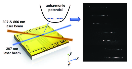
Figure 1: Ion string used as the potential probe. An linear ion chain is trapped above the SET and Doppler-cooled by the 397-nm and 866-nm laser light. Every time the voltage on one of the dc electrodes is changed, the ion string will move to a new equilibrium position. The extension feature of the ion string allows us to probe the spatial field distribution.

This force is equal and opposite to external force provided by the confining potential, $F_{ext}(x_{i})$. The corresponding electric field intensity termed $E_{ext}(x_{i})$. Using the ion positions as interpolation points, the function $E_{ext}(x_{i})$ can be numerically integrated to give the instantaneous confining potential in 1D with a unimportant unknown integration constant. It should be mentioned that the force $E_{ext}(x_{i})$ contains two components, $E_{ext}(x_{i})=E_{t}(x_{i})+E_{s}(x_{i})$, where $E_{t}(x_{i})$ is due to all the dc electrodes and voltage dependent, $E_{s}(x_{i})$ is due to all the other unknown sources and voltage independent, which is also called stray field. The corresponding potentials are $\Phi_{t}$ and $\Phi_{s}$, respectively.

To measure the unit-voltage potential $\phi_{k}$ of the electrode $k$, the voltage on the electrode of interest is repeatedly varied by $\delta$ each time. The total potential $\Phi=\Phi_{t}+\Phi_{s}$ is depend on the voltage on the electrode of interest, $V_{k}$, and also on other electrodes. The constant voltages on other electrodes are collectively termed $V_{B}$. The unit-voltage potential provided by the electrode of interest can be calculated by

$$\phi_{k}(x)=\Phi_{t}(x,V_{k}=1,V_{B}=0)=$$ (4)

$$\left[\Phi(x,V_{k}+\delta,V_{B})-\Phi(x,V_{k},V_{B})\right]\times 1V/\delta.$$

Since the changed voltage $\delta$ will move the positions of the ions, $x_{i}$, the potential $\Phi_{t}(x,1,0)$ then can be calculated for all $x$ where the two data sets, $\Phi(x,V_{A}+\delta,V_{B})$ and $\Phi(x,V_{A},V_{B})$ overlap, with the help of data interpolation. Uncertainty due to numerical errors can be significantly decreased by averaging over the results of potentials for many values of $\delta$. The measurable regions is extend due to the fact that ion string moves as $\delta$ is varied.

Error analysis indicates that the interpolation step limited the accuracy of this method, since measurement uncertainty of the field is smaller for lower ion densities. However, the numerical interpolation become less accurate in the limit of low ion density. Besides, the averaged $\Phi_{t}(x,1,0)$ still can not guarantee the smoothness of potential, and therefore is not good in local field accuracy.

II.2 Basic Theory of The Optimization-Based Modeling Method

We now propose a data processing method based on numerical optimization, which minimize the error between model prediction and the experimental data. In this method, data interpolation is not necessary, since sampling points are chosen at where the ions located. Besides, our method combined the merit of analytical function and experimental measurement, i.e. smooth and accurate. The optimization algorithm allows the use of many different types of experimental data, which further improves the model accuracy.

To avoid integration, the unit-voltage electric field intensity of the $k^{th}$ electrode, $E_{k}(x,1,0)$ instead of $\Phi_{t}(x,1,0)$ is to be determined directly. This requires a parametric expression of the electric field intensity. For rectangular electrode, the partial derivatives of Eq.(1) provide a choice, where 1D distribution along the trap axis can be derived by letting $y$ to be the trap height and $z=0$. The parameters to be determined could be $x_{k1}$ and $x_{k2}$. However, this equation is too complicated for optimization purpose.

We found the 1D unit-voltage potential curve along $x$ axis derived either by Eq.(1) or BEM method can be well approximated by a unnormalized Lorentz curve with the error within only a few percent. As shown in Fig. (2a), the unite-voltage 1D potential of the $8^{th}$ electrode calculated by BEM method is fitted very well with Lorentz function. The axial component of the electric field strength also matches well with the first derivative of the Lorentz function, as shown in Fig. (2b).

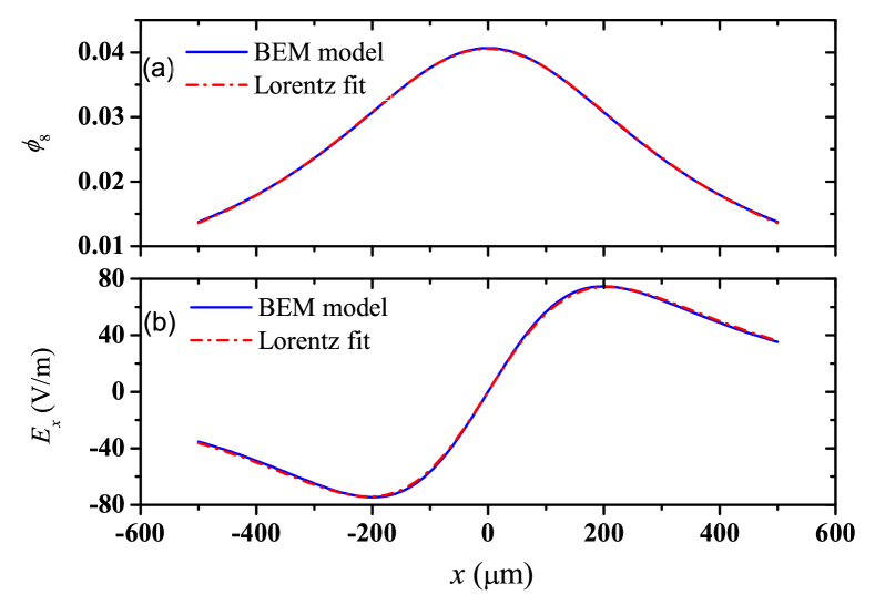
Figure 2: Lorentz fit of the 1D unit-voltage potential curve along $x$ axis. (a) The potential curve and (b) the axial component of the electric field strength. The blue solid lines are calculated by BEM method, and the red dashed lines are derived by the fitted Lorentz function.

Therefore, we start with a ansatz for the parametric expression of the electric field intensity of the $k^{th}$ rectangular electrode:

$$\phi_{k}(x)=\frac{A_{k}\gamma_{k}}{(x-x_{k})^{2}+\gamma_{k}^{2}}.$$ (5)

The free parameters $A_{k}$ and $\gamma_{k}$ are to be determined, and $x_{k}$ is the center position of the $k^{th}$ electrode. Then the $x$ component of electric field intensity can be calculated by $E_{k}(x)=-\partial\phi_{k}(x)/\partial x$. This set of parametric functions is then used to express the $x$ component of the electric field intensity $E(x)=\sum_{k=1}^{N}V_{k}E_{k}(x)+E_{s}(x)$. The basic idea of optimization method is to minimize the sum of squared errors of the predicted and measured trapping force $F_{ext}(x_{i})$ over all the ions under all the different voltage settings.

We will have to assume that the stray electric field keeps unchanged during the measurement. Since the trap region is relatively small, we take the second ansatz that the axial distribution of stray electric field is of the form

$$E_{s}(x)=ax^{2}+bx+c,$$ (6)

where, $a$, $b$ and $c$ are undetermined parameters.

Other than the equilibrium position of the ions string, the secular motion frequency data at different voltage settings can also be used to determine the model parameters. Unlike the equilibrium position of trapped ion, the secular motion frequency is related to the second derivative of the potential at the location of potential minimum, $D(x_{i})=\sum_{k=1}^{N}V_{k}D_{k}(x_{i})+D_{s}(x_{i})$ as follows:

$$\omega_{x}=\sqrt{\frac{eD(x_{i})}{M_{ion}}},$$ (7)

with $x_{i}$ the equilibrium position, and the notation $D_{k}(x_{i})=\frac{\partial^{2}\phi_{k}(x)}{\partial x^{2}}|_{x=x_{i}}$, $D_{s}(x_{i})=\frac{\partial^{2}\Phi_{s}(x)}{\partial x^{2}}|_{x=x_{i}}$.

Furthermore, the equilibrium position of a single ion trapped under certain voltages can be used as constrains for the solution. This position $x_{i}$ is determined in trap model by the root of $E(x_{i})=0$. Compared with the ion string data set, the single ion data set is much more accurate, since error only comes from the position uncertainty of the ion itself. But it is poorer in spatial extension.

Using data sets of different types and characteristics will modify the local field precision. To fully utilizing all these data sets, the modeling process can now be summarized as a multi-objective optimization problem with the objective function:

$$t_{1}=\sum_{i,j}|\widetilde{E}_{ext}(U_{j},x_{j,i})-E_{s}(x_{j,i})-\sum_{k=1}^{N}V_{j,k}E_{k}(x_{j,i})|^{2}$$

$$t_{2}=\sum_{j}\bigg{|}\widetilde{\omega}_{x}(U_{j},x_{j})-\sqrt{\frac{eD_{s}(x_{j})}{M}+\sum_{k=1}^{N}\frac{eV_{j,k}D_{k}(x_{j})}{M}}\bigg{|}^{2}$$

subject to   $|E_{s}(x_{j})+\sum_{k=1}^{N}V_{j,k}E_{k}(x_{j})|\leq\Delta\widetilde{E}$.

Where, $x_{j,i}$ ($x_{j}$) is the position of $i^{th}$ ion in a linear chain ($i$ omitted for a single ion) under the $j^{th}$ voltage settings $U_{j}$, in which the $k^{th}$ electrode is of the voltage $V_{j,k}$, $\widetilde{E}_{ext}$ and $\widetilde{\omega}_{x}$ are the position dependent measured electric field intensity and secular frequency under certain voltage settings, $N$ is the number of electrodes. The undetermined parameters $A_{k}$ and $\gamma_{k}$ are contained in the expressions of $E_{s}$, $E_{k}$, $D_{s}$ and $D_{k}$. The constraint restrict the predicted position of a single ion located at the measured $x_{i}$, with a field intensity uncertainty $\Delta\widetilde{E}=M\widetilde{\omega}_{x}^{2}\Delta x/e$ due to the random error of the ion position $\Delta x$.

The number of undetermined parameters is $2N+3$, which is increased linearly with the number of electrodes involved. For the case that working electrode pairs less than 10, as illustrated in this work, the problem can be solved by global optimization algorithm, such as Differential Evolution. For larger number of electrodes, we suggest that the electrodes should be divided into several groups, each group of the electrodes should be able to trap ions and then can be experimentally modeled separately. By this way, the optimization process will be more efficient. Besides, the experimental period will be shorter, and the assumption of constant stray field should be better satisfied.

III Experimental scheme

Our linear SET is a "five wire" trap. The apparatus is described in reference[38]. The trap consists of fifteen pairs of dc electrodes, as shown in Fig.[3]. The dc electrodes named from $1a(b)$ to $15a(b)$ are used for axial confinement. The other electrodes RF1(2) and GND provide the transverse confinement. The radio-frequency loaded to the trap is about $\Omega_{rf}=2\pi\times 22.7$ MHz, and lead to a transverse trap frequency about $2\pi\times 2.6$ MHz. Such a tight confinement allows us to push the ion crystal move along the trap axis while do not vary the trapping height too much. The axial confining potential is provided by 9 channels of the DAC device, with the output range $(-10V\sim 10V)$. Only the central nine (i.e. $4a(b)$ to $12a(b)$) out of the fifteen pairs of DC electrodes are used, with the rest pairs grounded.

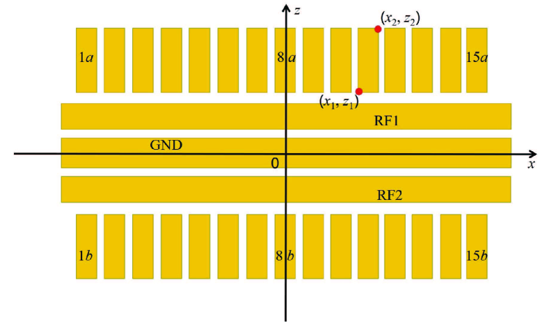
Figure 3: Schematic diagram of the "five wire" linear ion trap. The dc electrodes located at the $y=0$ plane are labeled from $1a(b)$ to $15a(b)$ above (below) the radiofrequency electrodes RF1(2) and GND.

The ${}^{40}\text{Ca}^{+}$ ions are loaded by three step photo-ionization of the Ca atoms using 423-nm and 732-nm laser light[39], after heating the atom oven. A linear chain of the ${}^{40}\text{Ca}^{+}$ ions is confined in an anharmonic potential along trap axis. The minimum spacing between adjacent ions is above 10 $\mu$m to ensure the field sensing sensitivity. The linear chain is Doppler cooled with 397- and 866-nm laser light. We have two 397-nm laser beams, one is along the $(1,0,0)$ dirction which provides cooling in the $x$ direction. The other is slightly tilted from $(1,0,1)$ direction, providing most cooling component in the $z$ and $x$ direction, and only a little component in the $y$ direction. It is not important since the sensitive surface of the camera is perpendicular to this direction. Cooling ions to the Doppler-limit is not necessary, but minimize the micromotion is important. When the voltages are identically applied to the "$i$a" and "$i$b" electrodes, micromotion is negligible in the $z$ direction in our trap, since we found the position of the ions observed on the camera is independent of the rf power. Coarse micromotion reduction in the $y$ direction is achieved by adjusting the height of the ions above the trap until the images of the individual ions are best localized on the camera. The number of ions in the chain will decrease gradually due to the collision with residual gas in the vacuum chamber. Loading process will be launched to keep the ion number within 6 to 19 in a experiment.

A pair of the electrodes labeled "$i$a" and "$i$b" ($4\leq i\leq 12$) are provided with the same voltage, and the unit-voltage potential are determined by pairs. In the crystal data set acquisition stage, voltage on each $i^{th}$ pair are repeatedly updated with a voltage increment of $\delta_{i}\sim 0.02V$ while keeping all the other voltages unchanged, pushing the ion crystal move across the region of interest ($\sim 280\mu$m, limited by the beam width of diagonal 397-nm laser). In this way, the unit-voltage electric field intensity of the pair of electrode "$i$a" and "$i$b" can be calculated as a whole. Note that keeping the $\delta_{i}$ constant for a specific $i^{th}$ electrode and the other voltages constant is necessary for the interpolation method, but not for ours. Instead, to cover wider operating voltage range and mitigate systematic error, change voltages on different electrodes simultaneously is preferred. In contrast, recording all the voltages on each electrode is necessary for the latter but not for the former. We follow all the requirements of two methods in the experiment, such that results of the two methods can be compared using the same set of experimental data.

Every time the voltage of the dc electrode is updated, an image of the linear ion crystal is photographed by an Electron-Multiplying charge-coupled device (EMCCD iXon Ultra 888). The custom-made lens provide about 19 times amplification, which results in resolution of $0.676\mu m$ per pixel size. The exact magnification of the system is calibrated by taking the image of a trap electrode with known width, and checked by the image of two trapped ions, whose distance can be precisely calculated by the measured trap frequency.

Position of a ion in the crystal under voltages $U_{j}$ is determined by 2D Gaussian fit. For each ion $i$, we first derive the center of mass position, then the image is divided into sections, each contains only one ion, and the dividing line is in the middle of two adjacent ions. Then the 2D Gaussian fit is applicable for each ion. The position error is estimated by the fitting quality, to be less than 0.12 $\mu$m. These positions $x_{j,i}$ are used to calculate the electric field intensity $\widetilde{E}_{ext}(U_{j},x_{j,i})$ by Eq. (3) and $E=F/e$.

The procedure of acquiring the equilibrium position of a single ion $x_{j}$ under certain voltages $U_{j}$ is just similar. After changing the voltage settings, the image of a single trapped ion is taken, and 2D Gaussian fit is used to determine the ion position. During the measurement, the exact position of both the ion trap and the image system are kept unchanged.

The secular frequencies $\widetilde{\omega}_{x}(U_{j},x_{j})$ are then measured by resonant excitation, with the equilibrium positions and voltage settings recorded at the same time. The excitation signal provided by a sine wave generator is connected to the outermost dc electrode. To achieve uttermost accuracy in secular frequency, we use a single trapped ion and very weak resonant excitation signal. Fluorescence level will change when the excitation frequency sweep across resonance point. The measurement uncertainty is less than $\pm 0.5$kHz.

In our experiment, the number of undetermined parameters is as large as 21, therefore the data sets should be large enough to reduce the parameter uncertainty. We take over 30 pictures for each pair of electrodes under different voltages, each picture contains 6 to 19 ions, together with 20 secular frequencies and 2 single trapped ion’s positions (more should be better). The total number of data points is up to 3484, which are all used in the optimization method. The interpolation method, however, can only make use of part of them. Except the secular frequencies and single trapped ion’s positions, the position data near the ends of the ion chain are not useful, since the number of overlapped samples are not enough for average to reduce the random error. For comparison, both the interpolation method and our optimization one are used to derive the unit-voltage field intensity for each pair of dc electrodes and also for the stray field.

IV Result

We first use the interpolation method proposed by M. Brownnutt et al.[36] to calculate unit-voltage electric field intensity of the dc electrodes by pairs, using only the ion crystal data set. As is shown in black dotted lines in Fig. 4, random fluctuation of the derived field intensity is obvious, especially at the two ends of the region, where the samples for averaging is very few. For better modeling the trap we smooth these curves by fitting them with Lorentz function according to Eq.(5), but only restricted to data within $-110\sim 110\mu$m to avoid obvious errors, as is shown in blue lines in Fig. 4.

Also shown in this figure, the red lines are derived by the newly proposed optimization method, using all the collected data without discarding the ends. The optimization target $t_{1}$ and $t_{2}$ are combined and balanced with a weighting factor. Two positions of a single trapped ion under different voltages are used for constraint the solution.

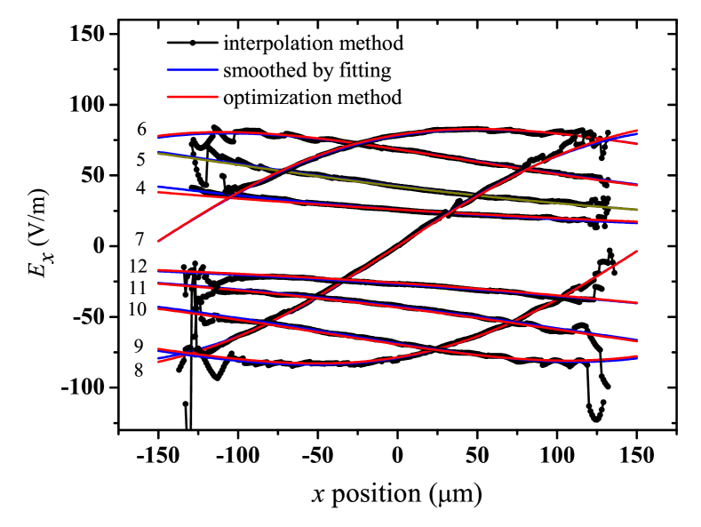
Figure 4: Unit-voltage electric field intensity curves of electrode $4-12$ derived by different methods. The curve correspond to the $i^{th}$ electrode is label by number $i$ to the left. The black solid lines with dots are derived by interpolation method. The discrete data within the range $(-110,110)\mu$m are fitted using the Lorentz function Eq. (5) to be the blue solid lines. The red solid lines are derived by optimization method, with all the experimental data included.

Stray electric field can also be derived. In the optimization method it is solved directly. But in the interpolation method, the stray electric field has been subtracted as a background. In this case, we calculate the residual error between measured electric field and the predicted one after all the unit-voltage electric field intensity has been derived, and all the data are taken into account by optimization method to determine the parameters of stray field in Eq.(6). The stray electric field strength along the axis are separately derived by two methods, as shown in Fig. (5). It is hard to say which curve is more accurate up to now. Both of the two curves indicate that the main source of stray field is not far from trap center. It may come from the constant voltage offset of certain electrode or the light charging effect due to the laser beams.

For simplicity, the unit-voltage field intensity of each electrode in blue (red) curves in Fig. 4 together with the stray field in blue (red) curve in Fig. 5 are referred as trap model established by interpolation (optimization) method.

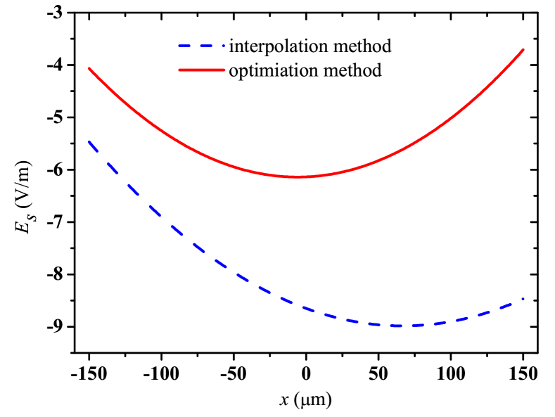
Figure 5: The stray electric field intensity $E_{s}$. The blue dashed line (red solid line) is derived by using the trap model according to interpolation (optimization) method.

To assess the accuracy of derived trap models, the equilibrium positions for certain number of ions and the secular frequencies under experimental voltages are calculated using the two trap models, and compared with the measured results. With the trap models derived above, one can simulate the equilibrium position of each ion in a linear chain either by simulated annealing method[40] or by molecular dynamics simulation[41]. We use the velocity-verlet algorithmis for 1D molecular dynamics simulation, and large damping is applied to speed up the equilibrium process.

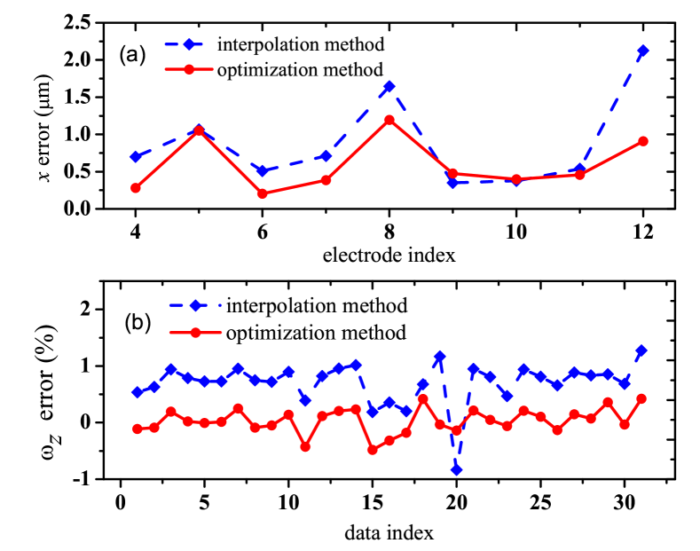
Figure 6: Errors of the $x$ positions and axial secular motion frequency predicted by two different trap models. (a) Mean errors of the predicted $x$ positions. The position errors of ions belong to the same voltage-varying electrode are averaged and shown with the corresponding electrode index. (b) Errors of the axial secular frequencies, with the $x$ axis represents the index of measured data. The blue dashed line with diamond (red solid line with dot) is according to the trap model derived by interpolation (optimization) method.

For each electrode $k$, we choose five voltage settings with different $V_{k}$ for molecular dynamics simulation. The five chosen $V_{k}$ include the maximum and minimum experimental values with the spacings as evenly as possible. The simulated equilibrium positions then are compared with the measured ones. The position errors of the ion belongs to the same voltage-varying electrode are averaged and shown in Fig. 6(a). Obviously, the errors are generally smaller using the model derived by optimization method than the one by interpolation. The worst error is about 1.2 $\mu$m for optimization method and 2.2 $\mu$m for interpolation method. And we found the errors are relatively larger for the $5^{th}$, $8^{th}$ and $12^{th}$ electrodes, for both of the two trap models. It indicates that there are some systematic errors in these model. We guess it comes from the assumption that the stray electric field keeps constant during the data acquisition period. Since the Ca oven are repeatedly turned on as well as the mW-level 423-nm photo-ionization laser to replenish the ${}^{40}\text{Ca}^{+}$. These operations may change the status of atomic coating and photo-induced charging up, which lead to variation of the stray field. This is the major drawback of the optimization method.

Fig. 6(b) shows the relative errors of predicted axial secular frequencies calculated using Eq. (7) for the two different models. Note that secular frequencies of the first 20 points are used to calculate target $t_{2}$ for optimaization, and the last 11 ones are just for check. The general trend of the two curves are very similar, but the errors derived by interpolation method has a offset of about $0.75\%$. There are good reasons to believe that the contribution of optimization target $t_{2}$ provide the suppression of this offset error. The trap model derived by optimization method shows high accuracy in predicting the secular motion frequency, with the error all below 0.5$\%$. Robustness also show when the trapping conditions are extended beyond the experimental region where we derive the trap model, e.g. secular frequencies used for optimization are ranged from 190 to 380 kHz, when it extended to 600kHz, the error of predicted frequency is still within 0.5$\%$.

V Conclusion And Discussion

A method has been presented to derive a smooth and accurate SET potential model based on multi-objective optimization method. This method combines the advantages of BEM simulation and experimental measurement, namely, highly curve smoothness and model accuracy. It naturally allow utilizing many different types of data, such as positions of ions in strings, secular frequencies and positions of single trapped ions under different trapping voltages. Therefore, it can mitigate systematic errors of different sources, and promise higher accuracy in the prediction of trap frequency and spatial field than any existing method. The higher accuracy is verified by comparing the errors of predicted equilibrium positions and the secular frequencies with those derived by the existing interpolation method.

Our method relies on the parametric expression of electric field intensity. The Lorentz function is found to be accurately enough for rectangular electrode in this work. Although this method is developed in the SET system, we believe it can also work for segmented 3D traps, except that the empirical expression of electric potential should be replaced. Our method generally requires that the stray field keeps constant during the data acquisition period, and then the 1d stray electric field intensity can be determined. If too much electrodes are involved, the global optimization algorithm will become less efficient, and the experimental period will last longer. In this case, the stray field are more tend to change. This can be solved by dividing the electrodes into several groups and each group of electrodes could be modeled separately.

This method can be extend to determine 2D even 3D potential, in principle. The ability to establish accurate trap model provide a practical tool for precisely trapping potential control, which may find application in ion transport and multi-ion based quantum precision metrology.