Topological Kondo Superconductors

Abstract

Spin-triplet $p$-wave superconductors are promising candidates for topological superconductors. They have been proposed in various heterostructures where a material with strong spin-orbit interaction is coupled to a conventional $s$-wave superconductor by proximity effect. However, topological superconductors existing in nature and driven purely by strong electron correlations are yet to be studied. Here we propose a realization of such a system in a class of Kondo lattice materials in the absence of spin-orbit coupling and proximity effect. Therein, the odd-parity Kondo hybridization mediates ferromagnetic spin-spin coupling and leads to spin-triplet resonant-valence-bond ($t$-RVB) pairing between local moments. Spin-triplet $p\pm ip^{\prime}$-wave topological superconductivity is reached when Kondo effect co-exists with $t$-RVB. We identify the topological nature by the non-trivial topological invariant and the Majorana fermions at edges. Our results offer a comprehensive understanding of experimental observations on UTe₂, a U-based ferromagnetic heavy-electron superconductor.

I Introduction

Searching for topological superconductors (TSc) and the corresponding self-dual charge neutral Majorana zero modes associated with their excitations at edges has become one of the central problem in condensed matter physics [1, 2]. Theoretical proposals and experimental realizations of TSc are mostly heterostructure combining strong spin-orbit coupled materials and conventional superconductors by proximity effect [3, 4, 5]. The emergence of the topological edge states in such systems can be explained in terms of the single-particle band structure without considering many-body electron correlations. Recently, the search for topological phases of matter has focused on a more intriguing class of materials that exist in nature. Their topological properties are driven by strong electron correlations instead of the proximity effect. Kondo effect, describing the screening of a local spin moment by conduction electrons, is a well-known strong correlation between electrons existing in heavy electron compounds. The Kondo-mediated topological phases of matter have been studied in the context of topological Kondo insulators [6, 7, 8] and topological Kondo semi-metals [9], where the topological properties are driven by either the odd-parity Kondo hybridization or by the Kondo hybridization with strong spin-orbit coupling.

Spin-triplet $p$-wave superconductors are known to be the prime candidates for TSc. However, they are scarce in nature. While it is still debatable for SrRu₂O₄ [10, 11, 12], more convincing evidence for $p$-wave triplet superconductivity was observed in noncentrosymmetric superconductor BiPd from phase-sensitive measurement [13]. More recently, signatures of triplet chiral $p$-wave superconductivity were observed in heavy-electron Kondo lattice compound UTe₂ at the edge of ferromagnetism, possibly marking the first example of topological superconductor induced by the strongly correlated Kondo effect [14, 15, 16, 17].

Motivated by these discoveries, in this paper, we propose a distinct class of triplet $p$-wave superconductors in the absence of spin-orbit coupling or proximity effect/heterostructure [18] in a two-dimensional Kondo lattice model driven by odd-parity Kondo hybridization. We start from the Anderson lattice model (ALM) with odd-parity hybridization, which occurs between $d$- and $f$-orbital electrons in various heavy-fermion compounds [6, 7, 8]. Via the Schrieffer-Wolff transformation [19, 20], we derive an effective Kondo lattice model with odd-parity hybridization. Furthermore, by integrating out the conduction electron degrees of freedom, an effective ferromagnetic RKKY interaction is generated. We explore the mean-field phase diagram of this ferromagnetic Kondo-Heisenberg model. In the fermionic mean-field approach, the ferromagnetic RKKY coupling describes the $p$-wave ($S_{z}=\pm 1$) $t$-RVB spin-liquid state. A time-reversal invariant topological superconducting phase is reached when the Kondo effect co-exists with the $p$-wave $t$-RVB order parameter. The topological nature of this superconducting phase is manifested by the non-trivial $Z_{2}$ topological Chern number of the bulk band and by the existence of helical Majorana zero modes at the edges of a finite-sized ribbon. Our results offer a qualitative and some quantitative understanding of the spin-triplet superconductivity recently observed in UTe₂ (see Discussions).

II Model

II.1 Anderson lattice model with odd-parity hybridization

We start with the odd-parity Anderson lattice model (ALM) on a two-dimensional (2D) square lattice, which has been shown to exhibit topologically non-trivial states [6, 7, 8]:

$$H_{PAM}=H_{c}+H_{f}+H_{cf},$$ (1)

where $H_{c}=\sum_{\mathbold{k},\sigma=\uparrow,\downarrow}\varepsilon_{\mathbold}{k}c^{\dagger}_{\mathbold{k}\sigma}c_{\mathbold{k}\sigma}$ describes the hopping of electrons in the $d$ orbits with orbital angular momentum $l=2$ and dispersion $\varepsilon_{\mathbold}{k}=-2t(\cos k_{x}+\cos k_{y})-\mu$. The Hamiltonian $H_{f}$ of the more localized electron in the $f$ orbits with orbital angular momentum $l=3$ is given by

$$H_{f}=\sum_{i,\sigma}\left[\varepsilon_{f}f^{\dagger}_{i\sigma}f_{i\sigma}+\frac{U}{2}n_{i\sigma}^{f}n_{i,-\sigma}^{f}\right],$$ (2)

where $\varepsilon_{f}$ denote the energy level of the $f$-electron, and $U$ is the repulsive on-site Coulomb potential (the Hubbard-$U$ term). Hybridization of the local and conduction electrons is described by

$$H_{cf}=\sum_{\langle i,j\rangle}\sum_{\sigma,\sigma^{\prime}=\uparrow\downarrow}V_{ij}^{\sigma\sigma^{\prime}}c^{\dagger}_{i\sigma}f_{j\sigma^{\prime}}+H.c..$$ (3)

To conserve the parity symmetry of hybridization between electrons with their angular momentum quantum numbers differing by one, $V_{ij}^{\sigma\sigma^{\prime}}$ have to be odd under parity transformation. This restriction results in the hybridization having to depend on sites and spins [6, 7, 8]:

$$V_{ij}^{\sigma\sigma^{\prime}}\equiv V_{\hat{\alpha}}^{\sigma\sigma^{\prime}}=iV\nu_{\hat{\alpha}}\sigma_{{\alpha}}^{\sigma\sigma^{\prime}},$$ (4)

distinct from the well-known onsite and spin-conserving Anderson hybridization. In Eq. (4), $\nu_{ij}$ satisfies $\nu_{ij}\equiv\nu_{\hat{\alpha}}=-\nu_{ji}$ with $\hat{\alpha}\equiv i-j\in\ \hat{x},\hat{y}\,(\alpha\in x,y)$ on a 2D square lattice, and $\sigma_{\alpha}$ denotes the Pauli matrix of the $\alpha$ component.

II.2 The effective odd-parity ferromagnetic Kondo lattice model

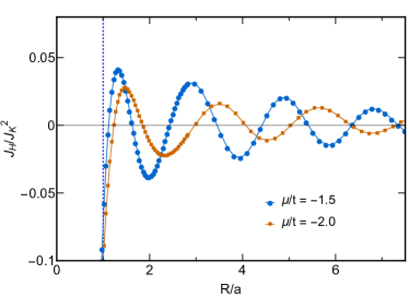
Figure 1: The effective RKKY coupling $J_{H}$ (normalized with $J_{K}^{2}$) as a function of $R/a$ for different chemical potentials $\mu$. $J_{H}$ is computed by Eq. (7) with $\mathbold{R}_{ij}\parallel(1,1)$ and $a=1$ being chosen.

In this paper, we focus on the competition of the Kondo and the magnetic interaction among impurities–the Doniach scenario [21]. We, therefore, derive the effective Kondo-Heisenberg lattice Hamiltonian from ALM in the Kondo limit where the vacant and doubly-occupied states are projected out from the entire Hilbert space, namely $1=\sum_{\sigma}f^{\dagger}_{i\sigma}f_{i\sigma}$. The low-energy effective Kondo term from the odd-parity ALM of Eq. (1) can be derived by applying the Schrieffer-Wolff transformation (SWT) [19, 20, 22], yielding

$$H_{K}=(-J_{K}) \sum_{i}\sum_{\sigma\sigma^{\prime}}\sum_{\sigma^{\prime\prime}\sigma^{\prime\prime\prime}}\sum_{\alpha,\alpha^{\prime}}\left(i\nu_{\hat{\alpha}}\sigma_{\alpha}^{\sigma\sigma^{\prime}}c_{i+\hat{\alpha},\sigma}^{\dagger}f_{i\sigma^{\prime}}\right)$$

$$\times\left(i\nu_{\hat{\alpha}^{\prime}}\sigma_{\alpha^{\prime}}^{\sigma^{\prime\prime}\sigma^{\prime\prime\prime}}f_{i\sigma^{\prime\prime}}^{\dagger}c_{i-\hat{\alpha}^{\prime},\sigma^{\prime\prime\prime}}\right)$$ (5)

with $J_{K}=\frac{V^{2}}{U+\varepsilon_{f}-\varepsilon_{F}}+\frac{V^{2}}{\varepsilon_{F}-\varepsilon_{f}}>0$ (see Appendix A). The Kondo-like term of Eq. (5) describes the screening of an impurity by its neighboring conduction electrons, distinct from the conventional (on-site) Kondo term.

Here, we go beyond the topological Kondo insulating phase by further deriving the magnetic RKKY interaction among the local $f$-fermions. By perturbatively expanding the Kondo term to second order [23, 24, 22], we obtain the effective RKKY-like interaction between the local $f$ fermions $f_{i\sigma}$,

$$H_{J}= \sum_{i,j}\sum_{\sigma,\sigma^{\prime}}J_{ij}f_{i\sigma}^{\dagger}f_{j\sigma^{\prime}}^{\dagger}f_{j\sigma}f_{i\sigma^{\prime}}$$

$$= \sum_{\left\langle i,j\right\rangle}J_{ij}\left(f_{i\uparrow}^{\dagger}f_{j\uparrow}^{\dagger}f_{j\uparrow}f_{i\uparrow}+f_{i\downarrow}^{\dagger}f_{j\downarrow}^{\dagger}f_{j\downarrow}f_{i\downarrow}\right)$$

$$+\sum_{\left\langle i,j\right\rangle}\frac{J_{ij}}{2}\left(f_{i\uparrow}^{\dagger}f_{j\downarrow}^{\dagger}+f_{i\downarrow}^{\dagger}f_{j\uparrow}^{\dagger}\right)\left(f_{j\downarrow}f_{i\uparrow}+f_{j\uparrow}f_{i\downarrow}\right)$$

$$-\sum_{\left\langle i,j\right\rangle}\frac{J_{ij}}{2}\left(f_{i\uparrow}^{\dagger}f_{j\downarrow}^{\dagger}-f_{i\downarrow}^{\dagger}f_{j\uparrow}^{\dagger}\right)\left(f_{j\downarrow}f_{i\uparrow}-f_{j\uparrow}f_{i\downarrow}\right),$$ (6)

where

$$J_{ij}\equiv J_{H}( R)=\frac{16J_{K}^{2}}{\mathcal{N}_{s}^{2}}\sum_{\varepsilon_{\mathbold{k}}<\mu}\sum_{\varepsilon_{\mathbold{k}^{\prime\prime}}>\mu}\frac{e^{i\left(\mathbold{k}-\mathbold{k}^{\prime\prime}\right)\cdot\mathbold{R}_{ij}}}{\varepsilon_{\mathbold{k}}-\varepsilon_{\mathbold{k}^{\prime\prime}}}$$

$$\times\left(\sin^{2}k_{x}+\sin^{2}k_{y}\right)\left(\sin^{2}k_{x}^{\prime\prime}+\sin^{2}k_{y}^{\prime\prime}\right)$$ (7)

denotes the effective coupling of the spinons of sites $i$ and $j$ with $R\equiv|\mathbold{R}_{ij}|\equiv|\mathbold{r}_{i}-\mathbold{r}_{j}|$. The $H_{J}$ term of Eq. (6) can be re-expressed as a linear combination of a spinon pair wave function with total spin $S=0$ (spin-singlet) and $S=1$ (spin-triplet). Note that the associated effective spinon coupling of the spin-triplet channel is opposite to that of the spin-singlet. When $H_{J}$ is expressed in terms of fermion pair with different spins, Eq. (6) is reminiscent of the conventional Heisenberg interaction $\mathbold{S}_{i}\cdot\mathbold{S}_{j}=-\frac{1}{2}\left(f_{i\uparrow}^{\dagger}f_{j\downarrow}^{\dagger}-f_{i\downarrow}^{\dagger}f_{j\uparrow}^{\dagger}\right)\left(f_{i\downarrow}f_{j\uparrow}-f_{i\uparrow}f_{j\downarrow}\right)+\frac{1}{4}n_{i}^{f}n_{j}^{f}$, except for the difference in the constant coefficients of the pair operators. As expected, the RKKY coupling $J_{ij}$ in Eq. (7) shows an oscillatory behavior in $R$, accompanied by a decrease in its magnitude with increasing $R$, similar to the behavior of the conventional RKKY coupling. Due to the rapid attenuation of $J_{ij}$, we only consider the dominated nearest-neighbor interaction and assume $J_{ij}$ to be spatially homogeneous, i.e. $J_{ij}\to J(R=a)\equiv J_{H}$. Furthermore, when $R=a$, we find the effective RKKY coupling is attractive (or of the ferromagnetic type), i.e., $J_{H}<0$ (see Fig. 1), which energetically favors the spin-triplet pairing of spinons. On the other hand, the effective RKKY coupling in the spin-singlet channel shows repulsive interaction and can be neglected here since it is not energetically favorable. Lastly, on a two-dimensional lattice, the triplet spin state $|\uparrow\downarrow\rangle+|\downarrow\uparrow\rangle$ does not exist since the corresponding structure factor is proportional to $k_{z}$, and $k_{z}=0$ is fixed here. Therefore, based on the above arguments, only the equal-spin states, $|\uparrow\uparrow\rangle$ and $|\downarrow\downarrow\rangle$, survive, and the $H_{J}$ term is reduced to

$$H_{J}\approx-\left|J_{H}\right|\sum_{\left\langle i,j\right\rangle}\left(f_{i\uparrow}^{\dagger}f_{j\uparrow}^{\dagger}f_{j\uparrow}f_{i\uparrow}+f_{i\downarrow}^{\dagger}f_{j\downarrow}^{\dagger}f_{j\downarrow}f_{i\downarrow}\right).$$ (8)

Combining $H_{K}$ and $H_{J}$ of Eqs. (5), (6) and (8), the effective Kondo-Heisenberg lattice model with odd-parity Kondo hybridization reads $H_{FKH}=H_{0}+H_{\lambda}+H_{K}+H_{J}$. Here, $H_{\lambda}=-\sum_{i}i\lambda_{i}\left[\sum_{\sigma}(f^{\dagger}_{i\sigma}f_{i\sigma})-1\right]$ enforces the singly occupied local $f$-spinons with $\lambda_{i}$ being the Lagrange multiplier. The Hamiltonian $H_{FKH}$ offers a platform for discovering a distinct class of topological superconducting states induced by electron correlations via collaboration between the ferromagnetic RKKY coupling and the Kondo effect. To facilitate our numerical calculations of the mean-field phase diagram, we treat $J_{K}$ and $J_{H}$ as independent couplings here since it is more convenient to explore the phase diagram by tuning the ratio of $J_{K}/J_{H}$ [25, 26]. In experiments, varying the non-thermal parameter can be expected to follow a certain trajectory of $J_{K}/J_{H}$ in the phase diagram.

III Mean-field treatment of the effective Kondo-Heisenberg-like model

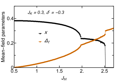
Figure 2: The zero-temperature mean-field solutions of $t$-RVB order parameter $\Delta_{t}$ (brown) and the Kondo correlation $x$ (black) as a function of $J_{H}$. We fix $J_{K}=0.3$ and doping of the conduction band $\delta=-0.3$ ($30$ percent hole doping). Without loss of generality, we set $t=1$. This plot reveals a (co-existing) superconducting ground state with $x\neq 0,\,\Delta_{t}\neq 0$ for $0<J_{H}\lesssim 2.5$ and a pure $t$-RVB phase where $x=0,\,\Delta_{t}\neq 0$ when $J_{H}\gtrsim 2.52$. A pure Kondo phase ($x\neq 0,\,\Delta_{t}=0$) only exists at $J_{H}=0$.

We now employ a mean-field analysis on the above effective Kondo-Heisenberg-like Hamiltonian with an effective ferromagnetic RKKY interaction and odd-parity Kondo hybridization.

Via performing Hubbard-Stratonovich transformation, $H_{K}$ and $H_{J}$ of Eqs. (5) and (6) can be factorized as

$$H_{K}\to\sum_{i,\alpha}\sum_{\sigma\sigma^{\prime}}\left[\chi^{\dagger}_{i}\left(i\nu_{\hat{\alpha}}\sigma_{\alpha}^{\sigma\sigma^{\prime}}f_{i\sigma}^{\dagger}c_{i-\hat{\alpha},\sigma^{\prime}}\right)+H.c.\right]$$

$$\qquad\qquad+\sum_{i}\frac{|\chi_{i}|^{2}}{J_{K}},$$

$$H_{J}\to\sum_{\left\langle i,j\right\rangle}\left[\Delta^{\uparrow}_{t}(i,j)f_{i\uparrow}^{\dagger}f_{j\uparrow}^{\dagger}+\Delta^{\downarrow}_{t}(i,j)f_{i\downarrow}^{\dagger}f_{j\downarrow}^{\dagger}+H.c.\right]$$

$$\qquad\qquad+\sum_{\langle i,j\rangle}\frac{\left|\Delta^{\uparrow}_{t}(i,j)\right|^{2}+\left|\Delta^{\downarrow}_{t}(i,j)\right|^{2}}{J_{H}}$$ (9)

where the mean-field values of the bosonic Hubbard-Stratonovich fields, $\chi_{i}$ and $\Delta^{\sigma}_{t}(i,j)$ ($\sigma=\uparrow,\downarrow$), represent the order parameters of the Kondo correlation and the $S_{z}=\pm 1$ spin-triplet RVB bonds between two adjacent up/down spins, respectively.

To describe the Kondo-screened Fermi-liquid state, we allow the $\chi_{i}$ field to acquire uniformly Bose condensation over the real space; hence, $\chi_{i}$ can be expressed as $\chi_{i}\to x+\hat{\chi}_{i}$ with $x=(-J_{K}/\mathcal{N}_{s})\sum_{i\sigma\sigma^{\prime}\alpha}\langle i\nu_{\hat{\alpha}}\sigma_{\alpha}^{\sigma\sigma^{\prime}}f_{i\sigma}^{\dagger}c_{i-\hat{\alpha},\sigma^{\prime}}\rangle$ being the Bose-condensed stiffness of $\chi_{i}$ while $\hat{\chi}_{i}$ represents its fluctuations. The mean-field order parameter of the $t$RVB is given by $\Delta_{t}^{\sigma}=(-J_{H}/4\mathcal{N}_{s})\sum_{\langle i,j\rangle}\langle f_{j\sigma}f_{i\sigma}\rangle$. Since the ferromagnetic coupling is expected to favor spin-triplet $p$-wave pairing similar to superfluid helium-3 [27], we restrict ourselves to the $p$-wave pairing, i.e., $\Delta_{t}^{\sigma}(i,j)$ here is taken the $p$-wave form, see Eqs. (11) and (12) below. We further fix the Lagrange multiplier at the mean-field level via $i\lambda_{i}\to\lambda$ and neglect the fluctuations of $\lambda_{i}$, $\chi_{i}$, and $\Delta_{t}^{\sigma}$, leading to the following mean-field Kondo-Heisenberg-like Hamiltonian:

$$H_{MF} =\sum_{\mathbold{k},\sigma}\varepsilon_{\mathbold{k}}c_{\mathbold{k}\sigma}^{\dagger}c_{\mathbold{k}\sigma}+\sum_{\mathbold{k}\sigma}\lambda f_{\mathbold{k}\sigma}^{\dagger}f_{\mathbold{k}\sigma}$$

$$+\sum_{\mathbold{k}}\left[V_{1\mathbold{k}}f_{\mathbold{k}\uparrow}^{\ast}c_{\mathbold{k}\downarrow}+V_{2\mathbold{k}}f_{\mathbold{k}\downarrow}^{\ast}c_{\mathbold{k}\uparrow}+H.c.\right]$$

$$+\sum_{\mathbold{k}}\left[\Delta_{\mathbold{k}}^{\uparrow}f_{\mathbold{k}\uparrow}^{\dagger}f_{-\mathbold{k}\uparrow}^{\dagger}+\Delta_{\mathbold{k}}^{\downarrow}f_{\mathbold{k}\downarrow}^{\dagger}f_{-\mathbold{k}\downarrow}^{\dagger}+H.c.\right]$$

$$+\frac{8\mathcal{N}_{s}\Delta_{t}^{2}}{J_{H}}+\frac{\mathcal{N}_{s}x^{2}}{J_{K}}-\mathcal{N}_{s}\lambda,$$ (10)

where $V_{1\mathbold{k}}=2x\left(\sin k_{x}-i\sin k_{y}\right)$ and $V_{2\mathbold{k}}=2x\left(\sin k_{x}+i\sin k_{y}\right)$. The Fourier transformation for the second-quantized operator is defined as $\psi_{i\sigma}=\frac{1}{\sqrt{\mathcal{N}_{s}}}\sum_{\mathbold{k}}e^{-i\mathbold{k}\cdot\mathbold{r}_{i}}\psi_{\mathbold{k}\sigma}$. Note that the mean-field Kondo term of Eq. (10) is reminiscent of the topological Kondo insulator shown in Ref. [28]. In Eq. (10), $\Delta_{t}^{\sigma}(\mathbold{k})$ represents the gap structure of the spin-triplet $p$-wave RVB pairing in the momentum space for the spin-$\sigma$ sector, defined as $\Delta_{\mathbold{k}}^{\uparrow}=\Delta_{t}\left(-\sin k_{y}-i\sin k_{x}\right)$ and $\quad\Delta_{\mathbold{k}}^{\downarrow}=\Delta_{t}\left(\sin k_{y}-i\sin k_{x}\right)$ with $\Delta_{t}$ being denoted the mean-field pairing potential (see Appendix, Section II). This momentum-dependent gap structure for the up- and down-spin sectors correspond to the following real-space patterns of $\Delta^{\uparrow}_{t}(i,j)$ and $\Delta^{\downarrow}_{t}(i,j)$ of Eq. (9):

$$\Delta_{t}^{\uparrow}(i,j)\to\Delta^{\uparrow}_{t}(i,i+\hat{x})=-\Delta^{\uparrow}_{t}(i,i-\hat{x})=-\Delta_{t},$$

$$\qquad\qquad\quad\Delta^{\uparrow}_{t}(i,i+\hat{y})=-\Delta^{\uparrow}_{t}(i,i-\hat{y})=i\Delta_{t},$$ (11)

and

$$\Delta_{t}^{\downarrow}(i,j)\to \Delta^{\downarrow}_{t}(i,i+\hat{x})=-\Delta^{\downarrow}_{t}(i,i-\hat{x})=-\Delta_{t},$$

$$\Delta^{\downarrow}_{t}(i,i+\hat{y})=-\Delta^{\downarrow}_{t}(i,i-\hat{y})=-i\Delta_{t}.$$ (12)

Choosing $\Psi_{\mathbold{k}}=\left(\phi_{A\mathbold{k}},\phi_{B\mathbold{k}}\right)^{T}$ with the Nambu spinors defined by $\phi_{A\mathbold{k}}=\left(c_{\mathbold{k}\uparrow},\,\,c_{-\mathbold{k}\uparrow}^{\dagger},\,\,f_{\mathbold{k}\downarrow},\,\,f_{-\mathbold{k}\downarrow}^{\dagger}\right)^{T}$ and $\phi_{B\mathbold{k}}=\left(c_{\mathbold{k}\downarrow},\,\,c_{-\mathbold{k}\downarrow}^{\dagger},\,\,f_{\mathbold{k}\uparrow},\,\,f_{-\mathbold{k}\uparrow}^{\dagger}\right)^{T}$, the mean-field Hamiltonian $H_{MF}=\sum_{\mathbold{k}}\Psi_{\mathbold{k}}^{\dagger}\mathcal{H}_{\mathbold{k}}\Psi_{\mathbold{k}}+\mathcal{C}$ can be expressed as a summation of two decoupled $4\times 4$ matrices as follows

$$H_{MF} =H_{A}+H_{B}+\mathcal{C},$$

$$H_{A(B)} =\sum_{\mathbold{k}}\phi_{A(B)\mathbold{k}}^{\dagger}\mathcal{H}_{\mathbold{k}}^{A(B)}\phi_{A(B)\mathbold{k}}$$ (13)

with $\mathcal{C}\equiv\sum_{\mathbold}{k}\varepsilon_{\mathbold}{k}+\frac{8\mathcal{N}_{s}\Delta_{t}^{2}}{J_{H}}+\frac{\mathcal{N}_{s}x^{2}}{J_{K}}$, and

$$\mathcal{H}_{\mathbold{k}}^{A} =\begin{pmatrix}\frac{\varepsilon_{\mathbold{k}}}{2}&0&\frac{V_{2\mathbold{k}}^{\ast}}{2}&0\\ 0&-\frac{\varepsilon_{\mathbold{k}}}{2}&0&\frac{V_{2\mathbold{k}}}{2}\\ \frac{V_{2\mathbold{k}}}{2}&0&\frac{\lambda}{2}&\Delta_{\mathbold{k}}^{\downarrow}\\ 0&\frac{V_{2\mathbold{k}}^{\ast}}{2}&\Delta_{\mathbold{k}}^{\downarrow\ast}&-\frac{\lambda}{2}\end{pmatrix},\,\,$$ (14)

$$\mathcal{H}_{\mathbold{k}}^{B} =\begin{pmatrix}\frac{\varepsilon_{\mathbold{k}}}{2}&0&\frac{V_{1\mathbold{k}}^{\ast}}{2}&0\\ 0&-\frac{\varepsilon_{\mathbold{k}}}{2}&0&\frac{V_{1\mathbold{k}}}{2}\\ \frac{V_{1\mathbold{k}}}{2}&0&\frac{\lambda}{2}&\Delta_{\mathbold{k}}^{\uparrow}\\ 0&\frac{V_{1\mathbold{k}}^{\ast}}{2}&\Delta_{\mathbold{k}}^{\uparrow\ast}&-\frac{\lambda}{2}.\end{pmatrix}$$ (15)

The Hamiltonian Eq. (13) possesses time-reversal symmetry: $\mathcal{H}_{A}$ and $\mathcal{H}_{B}$ constitute the time-reversal partner of each other, i.e. $\Theta\mathcal{H}_{A(B)}\Theta^{-1}=\mathcal{H}_{B(A)}$ where the time-reversal operator $\Theta=\rho^{0}\otimes(-i\sigma^{y})K$ with $\sigma^{y}$ being the $y$-component Pauli matrix on the spin subspace, $\rho^{0}$ being a $2\times 2$ identity matrix on the orbital subspace while $K$ being the complex-conjugate operator. Under time-reversal transformation, the spin and quasi-momentum of conduction ($c$) and pseudofermion ($f$) operators are flipped: $\left(c_{\bm{k}\uparrow},\,c_{\bm{k}\downarrow},\,f_{\bm{k}\uparrow},\,f_{\bm{k}\downarrow}\right)\stackrel{{\scriptstyle\Theta}}{{\longrightarrow}}\left(c_{-\bm{k}\downarrow},\,-c_{-\bm{k}\uparrow},\,f_{-\bm{k}\downarrow},\,-f_{-\bm{k}\uparrow}\right)$. Meanwhile, our Hamiltonian respects charge-conjugation (particle-hole) symmetry: $\mathcal{P}\mathcal{H}_{\bm{k}}\mathcal{P}^{-1}=-\mathcal{H}_{-\bm{k}}$ where $\mathcal{P}\equiv\tau^{x}K$ is the particle-hole operator with $\tau_{x}$ being the $x$-component of the Pauli matrices on the particle-hole basis. Due to the odd-parity $p\pm ip^{\prime}$ RVB pairing of our model, the parity symmetry is broken here. Thus, our model Eq. (13) belongs to the DIII class of topological symmetry [29].

IV Results

IV.1 Mean-field phase diagram

The mean-field ground states are determined by minimizing the mean-field free energy per site $\mathcal{F}_{MF}=\frac{\mathcal{C}}{\mathcal{N}_{s}}-\frac{k_{B}T}{\mathcal{N}_{s}}\sum_{n\bm{k}}\ln\left[1+\exp\left(-\frac{E_{n\bm{k}}}{k_{B}T}\right)\right]$ with respect to the mean-field variables $q=(\lambda,\,x,\,\Delta_{t})$, i.e. $\partial\mathcal{F}_{MF}/\partial q_{i}=0$. Here, $E_{n\mathbold{k}}<0$ is the $n$-th band of $\mathcal{H}_{\mathbold{k}}$. The chemical potential $\mu$ is determined by the relation $\partial\mathcal{F}_{MF}/\partial\mu=-(1+\delta)$ with $\delta$ being the chemical doping of the $c$-electrons for which $\delta\lesseqqgtr 0$ is for $p/\text{un}/n-$ doped (half-filling corresponds to $\delta=0$). This leads to the following saddle-point equations at zero temperature,

$$\frac{1}{\mathcal{N}_{s}}\sum_{n\bm{k}}\frac{\partial E_{n\bm{k}}}{\partial x}+\frac{2x}{J_{K}}=0,$$

$$\frac{1}{\mathcal{N}_{s}}\sum_{n\bm{k}}\frac{\partial E_{n\bm{k}}}{\partial\Delta_{t}}+\frac{16\Delta_{t}}{J_{H}}=0,$$

$$\frac{1}{\mathcal{N}_{s}}\sum_{n\bm{k}}\frac{\partial E_{n\bm{k}}}{\partial\lambda}=0,$$

$$\frac{1}{\mathcal{N}_{s}}\sum_{n\bm{k}}\frac{\partial E_{n\bm{k}}}{\partial\mu}+\delta=0.$$ (16)

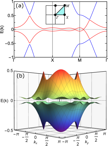
Figure 3: Figures (a) (red curves) and (b) show the bulk energy spectrum of the co-existing superconducting state near the Fermi level $\mu$. The Fermi level locates at $E(\bm{k})=0$. The coupling constants are $J_{K}=0.3$ and $J_{H}=1.0$. Inset of (a) displays the First Brillouin zone of a square lattice with indications of high-symmetry points $\Gamma,\,X,\,M$.

The ground-state phase diagram (Fig. 2) of our model is obtained by solving the saddle-point equations self-consistently. The phase diagram contains three distinct mean-field phases: a pure Kondo phase is found at $J_{H}=0$ where $x\neq 0$, $\Delta_{t}=0$. At the opposite limit where the RKKY interaction dominates, the ground state shows short-range magnetic correlation with $p$-wave spin-triplet RVB pairing ($\Delta_{t}\neq 0,\,x=0$). In the intermediate range of $0<J_{H}/J_{K}<(J_{H}/J_{K})_{c}$, we find a Kondo-$t$RVB co-existing (superconducting) phase with $x\neq 0$ and $\Delta_{t}\neq 0$, which can be explained via the mechanism of Kondo-stabilized spin liquid [30, 26]. The development of superconductivity in this co-existing phase requires higher-order processes involving both the Kondo and $t$-RVB terms: the mean-field $t$-RVB pairings of the local $f$ fermions provide preformed Cooper pairs. When the Kondo hybridization field $\chi$ gets Bose-condensed ($x\neq 0$), the local fermions delocalize into the conduction band and make the preformed $t$-RVB Cooper pairs superconduct [31]. These processes can be described by the effective mean-field Hamiltonian $H_{sc}=\sum_{\bm{k}}\left(\bar{\Delta}_{\bm{k}}^{\downarrow*}c_{-\bm{k}\downarrow}c_{\bm{k}\downarrow}+\bar{\Delta}_{\bm{k}}^{\uparrow*}c_{-\bm{k}\uparrow}c_{\bm{k}\uparrow}+H.c.\right)$, where the effective gap functions take the form $\bar{\Delta}_{\bm{k}}^{\downarrow*}=V_{1\bm{k}}V_{1,-\bm{k}}\Delta_{\bm{k}}^{\uparrow*}\sim x^{2}\Delta_{t}(\sin^{2}k_{x}+\sin^{2}k_{y})(\sin k_{x}-i\sin k_{y})$ and $\bar{\Delta}_{\bm{k}}^{\uparrow*}=V_{2\bm{k}}V_{2,-\bm{k}}\Delta_{\bm{k}}^{\downarrow*}\sim x^{2}\Delta_{t}(\sin^{2}k_{x}+\sin^{2}k_{y})(\sin k_{x}+i\sin k_{y})$ with the size of the superconducting gap being proportional to $x^{2}\Delta_{t}$. The superconducting gap function $\bar{\Delta}_{\bm{k}}^{\uparrow}$ we obtained here shows a $f$-wave-like pairing symmetry on a generic anisotropic (non-circular) 2D Fermi surface. Nevertheless, as we are taking the continuous limit of the conduction band here, $\bar{\Delta}_{\bm{k}}^{\uparrow}$ can be expressed as a product of $s$ and $p\pm ip^{\prime}$ pairing orders, i.e., $\bar{\Delta}_{\bm{k}}^{\uparrow/\downarrow*}\sim k^{2}(k_{x}\pm ik_{y})$ with $k^{2}\equiv k_{x}^{2}+k_{y}^{2}$ on a circular Fermi surface but only the $p\pm ip^{\prime}$ component plays a role here. Note that we find the co-existing superconducting state persists for an arbitrary small value of $J_{H}/J_{K}\to 0^{+}$. This is likely due to the overestimation of the co-existing phase at the mean-field level. Upon including fluctuations of the Kondo and $t$-RVB order parameters beyond the mean-field level, we expect a narrower co-existing superconducting phase. A first-order transition similar to the results found in Refs. [26, 32] is observed at the transition of the $t$-RVB and the co-existing superconducting phases (see Fig. 2). The bulk band structure in the co-existing superconducting state is shown in Fig. 3.

IV.2 Topological invariance

Figure 4: The left figure displays the electronic band structure of the coexisting superconductor state for a strip with $N_{y}=81$ described by $\mathcal{H}_{A}$ at $J_{K}/t=0.3$ and $J_{H}/t=1.0$. Three pairs of edge states with Dirac spectra are observed near $k_{x}=0$ (the pink curves). The edge states at zero energy correspond to the Majorana zero modes. Due to the time-reversal symmetry of the model, the band structure for a strip for $\mathcal{H}_{B}$ is identical to that of $\mathcal{H}_{A}$. The close-up band structures near three pairs of edge states (pink curves) on the top, middle and bottom bounded by the red squares are shown on the right figures.

We now address the topological properties of the coexisting superconducting state. Since this system is invariant under time-reversal transformation, the bulk topological properties of the coexisting Kondo-RVB superconducting state with $p\pm ip^{\prime}$ spin-triplet RVB pairing can be thus characterized by the $Z_{2}$ Chern number $c_{T}$ (or time-reversal polarization) [33, 34, 35], given by

$$c_{T}=\frac{c_{A}-c_{B}}{2}$$ (17)

with $c_{I}$ $(I\in A,B)$ being the Thouless-Kohmoto-Nightingal-den Nijs (TKNN) number [36] of $H_{I}$, defined as

$$c_{I}=\frac{1}{2\pi}\int_{\bm{k}\in\text{FBZ}}d\bm{S}_{\bm{k}}\cdot\left(\bm{\nabla}_{\bm{k}}\times\bm{\mathcal{A}}^{I}_{\bm{k}}\right).$$ (18)

The Berry’s connection $\bm{\mathcal{A}}^{I}_{\bm{k}}$ for $H_{I}$ is given by $\bm{\mathcal{A}}^{I}_{\bm{k}}\equiv i\sum_{n\in I}\langle u_{n\bm{k}}^{I}|\bm{\nabla_{\bm{k}}}|u_{n\bm{k}}^{I}\rangle$ with $|u_{n\bm{k}}^{I}\rangle$ being the normalized Bloch state of the $n$-th filled band for $H^{I}_{\bm{k}}$. We numerically calculate the TKNN numbers [37], $c_{A}$ and $c_{B}$, and find that $c_{A}=-c_{B}=1$ in the co-existing phase, indicating a topologically non-trivial $Z_{2}$ Chern number $c_{T}=1$. By the bulk-edge correspondence, we expect this co-existing superconducting state to support a pair of counter-propagating Majorana zero modes at the edges of a finite-sized strip. Further band structure calculations of our model on a strip in the following subsection confirm our expectation.

IV.3 Edge states of the coexisting Kondo-RVB spin-triplet $p\pm ip^{\prime}$-wave superconducting state

Figure 5: Figures (a) and (d) show the Bogoliubov excitation spectra of $\mathcal{H}_{A}$ and $\mathcal{H}_{B}$, respectively, near the chemical potential on a nano-strip with $N_{y}=81$ chains. Figures (b), (c) and (e), (f) demonstrate the probability density of the Majorana edge state wave functions of $\mathcal{H}_{A}$ and $\mathcal{H}_{B}$ as a function of atom position $y_{i}$, $\left|\gamma^{\Gamma}_{I,k_{x}}(y_{i})\right|^{2}$ with $I=A,B$ and $\Gamma=R,L$ (pink curves in (a) and (d)), at a fixed energy $E\equiv E(k_{x}=\pm 0.03)$. The probability density is described by $\left|\gamma^{\Gamma}_{I,k_{x}}(y_{i})\right|^{2}=\left(\left|u^{\Gamma}_{I,k_{x}}\right|^{2},\,\left|\bar{u}^{\Gamma}_{I,k_{x}}\right|^{2},\,\left|v^{\Gamma}_{I,k_{x}}\right|^{2},\,\left|\bar{v}^{\Gamma}_{I,k_{x}}\right|^{2}\right)(y_{i})$. The parameters are $J_{K}/t=0.3$, $J_{H}/t=1.0$, and doping $\delta=-0.3$. The edge states are of the helical type, as schematically represented in (g).

Figure 6: The finite-energy ($E(k_{x})>0$) Bogoliubov excitation spectra of (a) $\mathcal{H}_{A}$ (shown on top right in Fig. 5) and (d) $\mathcal{H}_{B}$. A pair of “helical” edge states is found to exist at finite energy [pink curve in (a) and (d)], and their probability densities are shown in (b) and (c), (e) and (f), respectively, at a fixed energy $E(k_{x}=\pm 0.22)$.

We now check whether our model would support helical Majorana zero modes at the edge of a finite-sized system. We shall examine our model’s band structures and edge-state wave functions on a finite-sized strip that extends infinitely along the $x$ direction but contains a finite number of lattice sites in $y$. The results are shown in Figs. 4 to 6. As shown in Fig. 4, gapless Dirac spectra of the Bogoliubov excitations around $k_{x}=0$ near zero energy are observed, exhibiting one of the typical features of topological edge states. The excitations can be effectively described by the linear-dispersed Hamiltonian $\tilde{H}_{I}=\sum_{k_{x}}v_{x}|k_{x}|\left(\gamma^{R\,\dagger}_{I,k_{x}}\gamma^{R}_{I,k_{x}}-\gamma^{L\,\dagger}_{I,k_{x}}\gamma^{L}_{I,k_{x}}\right)$ with

$$\gamma_{I,k_{x}}^{\Gamma}= \sum_{y_{i}}\left[u^{\Gamma}_{I,k_{x}}(y_{i})c_{k_{x},y_{i},\uparrow}+\bar{u}^{\Gamma}_{I,k_{x}}(y_{i})c_{-k_{x},y_{i},\uparrow}^{\dagger}\right.$$

$$\left.+v^{\Gamma}_{I,k_{x}}(y_{i})f_{k_{x},y_{i},\downarrow}+\bar{v}^{\Gamma}_{I,k_{x}}(y_{i})f_{-k_{x},y_{i},\downarrow}^{\dagger}\right]$$ (19)

with $u,\bar{u}$ and $v,\bar{v}$ being the coherent factors. In Eq. (19), $I\in A,B$, $\Gamma\in R,L$, and $\gamma^{R/L}_{A/B,k_{x}}$ represents the right/left-moving Bogoliubov quasiparticle of $\tilde{H}_{A/B}$. Here, $v_{x}$ in $\tilde{H}_{I}$ denotes the velocity. Due to time-reversal symmetry, $H_{A}$ is the time-reversal partner of $H_{B}$, and thus their spectra are identical. The low-energy eigenstates with Dirac spectra near $k_{x}=0$ for both $H_{A}$ and $H_{B}$ exhibit the typical property of edge states, as their probability densities accumulate mostly at the edges of strip, as shown in Fig. 5. Combining the directions of propagation inferred from the velocity $v_{x}\sim\partial E(k_{x})/\partial k_{x}$, we can classify these edge states into two groups, each of them constitutes a pair of counter-propagating edge states (see Fig. 5), revealing the nature of helical Majorana zero modes. The helical type of the Majorana zero modes is the consequence of time-reversal symmetry of our model, reminiscent of the well-known Kane-Mele model on a single-layered graphene [38, 39]. Remarkably, in addition to the Majorana fermions at zero energy, two pairs of counter-propagating edge-states are observed at finite energy, see Fig. 6. The two pairs of edge states correspond to the edge states of the topological Kondo insulator, where the spin-triplet RVB order parameter is absent ($\Delta_{t}=0$) [8, 7, 6].

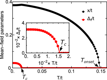
Figure 7: Plot of the temperature-dependent mean-field order parameters $x(T)/t$ and $\Delta_{t}(T)/t$ with $k_{B}=1$, $J_{K}/t=0.3$ and $J_{H}/t=1.0$ fixed. Inset shows the enlarged plot of $\Delta_{t}(T)$. The single-impurity Kondo temperature occurs at $T_{\text{onset}}/t\approx 0.16$ while the transition of superconductivity takes places at temperature $T_{c}/t\approx 0.015$.

V Discussions and Conclusions

We now discuss the application of our results for heavy-electron superconductors, particularly the Kondo lattice compound UTe₂. Experimental evidence indicates that this compound does not show long-range magnetic order and is in the vicinity of the ferromagnetic quantum critical point, exhibiting both strong ferromagnetic fluctuations, possibly due to magnetic frustrations induced by sub-leading antiferromagnetic fluctuations [40, 41], and Kondo screening [17, 14, 42]. The DFT+$U$ calculations indicate that the dynamics of electron bands and the physical properties of UTe₂ are dominated by the electrons near the quasi-two-dimensional (cylindrical) Fermi surface with weak $k_{z}$ dependence despite its 3D crystal structure [40]. Superconductivity is reached at $T_{c}=1.6$K, while the resistivity maximum observed at $T^{\star}\approx 15\sim 75$ K reveals signature of coherent Kondo scattering [43, 14], indicating $T^{\star}/T_{c}\approx 10\sim 50$. The superconductivity can, in general, co-exist and compete with the Kondo effect [17]. When a magnetic field is applied along the hard-magnetic axis $b$ of UTe₂ and before entering the superconducting phase, a correlated paramagnetic phase is observed below the temperature at which the magnetic susceptibility shows a broad maximum [44]. Similar spin-liquid behavior has been observed in the magnetic susceptibility of another heavy fermion compound CePdAl [45]. This similarity suggests this correlated paramagnetic phase may feature short-range magnetic order. Our theoretical framework based on competition and collaboration between a Kondo-screened and a ferromagnetic $t$-RVB spin-liquid states on a two-dimensional Kondo lattice is consistent with the above observations in UTe₂. It, therefore, constitutes a promising approach to account for its exotic phenomena. On the other hand, the chiral in-gap state, a signature of chiral topological superconductor, has been observed by scanning tunneling spectroscopy in the superconducting phase of UTe₂ [17]. Combining with the ferromagnetic fluctuations that are known to induce spin-triplet pairing, people believe UTe₂ is a promising candidate for the spin-triplet chiral topological superconductor [17, 14]. Furthermore, the superconducting phase co-existing with Kondo coherence in this material strongly suggests the role played by the Kondo effect in this possible topological superconductor. The topological Kondo superconducting state with equal-spin spin-triplet $p$-wave pairings we proposed here bears striking similarities to and strong relevance for the experimental observations on UTe₂: (i) the $d$- and $f$-orbitals electrons with their angular momentum quantum number differing by $1$ in the uranium atoms of UTe₂ likely give rise to the odd-parity Kondo effect [8, 7, 6], (ii) the $t$-RVB state in our theory may be considered as one possible realization of the short-ranged ferromagnetic fluctuations in UTe₂, (iii) the Kondo-$t$-RVB co-existing superconducting state we find here qualitatively agrees with the co-existence between superconductivity and Kondo effect observed in UTe₂, (iv) the high upper critical field exceeding the Pauli limit [14, 46] implies that the superconducting state of UTe₂ may have equal-spin Cooper pairs, and (v) the effective pairing $\overline{\Delta}_{\bm{k}}^{\sigma}$ formed in the conduction band mentioned in Section IV.1 shows characteristics of spin-triplet point-node gap structure [47]. Various characteristic temperature scales estimated from our mean-field calculations with $J_{H}/t=1.0$ and $J_{K}/t=0.3$ at finite temperatures agree reasonably well with experimental observations (see Fig. 7): The superconducting transition temperature $T_{c}$, theoretically determined from our mean-field analysis $T_{c}=\text{Min}[T(x=0),T(\Delta_{t}=0)]$, shows $T_{c}\approx 0.015t\approx 2.3\text{\,K}$ by taking estimated values of $t=150\,\text{K}$ and half-bandwidth $D=1.25t$ [42]. The Kondo coherent scale can be obtained by $T^{\star}=x^{2}(T=0)/D\approx 17.4\,\text{K}$ [48]. The ratio $T^{\star}/T_{c}\approx 8$ is in reasonable agreement with experimental observations. The onset temperature $T_{\text{onset}}$ of Kondo hybridization, which occurs at $x(T=T_{\text{onset}})=0$, displays $T_{\text{onset}}\approx 0.16t\approx 24\,\text{K}$, within the theoretically estimated range $10\text{K}<T_{\text{onset}}<100\text{K}$ by DMFT calculation [42]. Meanwhile, there have been evidences of TRS breaking in UTe₂ from the observed two superconducting transitions and a finite polar Kerr effect at $T<T_{c}$ [49], likely due to proximity to the ferromagnetic ordered phase. A number of theoretical attempts were proposed based on these observations [50, 51]. However, the observed single superconducting transition near ambient pressure and zero field [44, 52, 53] as well as the theoretically proposed unitary triplet pairing [40] suggest TRS may be preserved in UTe₂. Though our results shown above are obtained in the presence of TRS, the chiral $p$-wave superconducting state with chiral Majorana zero mode at edges is expected to occur here once a time-reversal breaking magnetic field is applied [54]. Our distinct predictions with and without fields serve as theoretical guidance for future experiments to distinguish the time-reversal breaking from time-reversal preserving triplet pairing states in UTe₂. Since the Kondo correlations stabilize the $t$-RVB spin liquid in the co-existing superconducting phase, it is expected to be robust against gauge-field fluctuations beyond the mean field. Our approach and results are distinct from the spin-triplet non-topological superconducting state recently proposed based on the Hund’s-Kondo coupling and $S_{z}=0$ $t$-RVB state to account for UTe₂ [51].

In conclusion, we propose a first realization of the topological superconductivity in the Kondo lattice model, a distinct class of topological superconductors due to purely strong electron correlations without employing spin-orbit coupling or proximity effect. A topological Kondo superconductor essentially constitutes of 1) itinerant $c$ and localized $f$ bands with different orbital quantum numbers, 2) strong Hubbard interaction of the $f$ electrons, 3) odd-parity Kondo hybridization of the $c$ and $f$ bands, and 4) the attractive exchange interaction of the $f$ electrons with spin-triplet correlations. Starting from the odd-parity Anderson lattice model, we obtain the unconventional type of Kondo hybridization and ferromagnetic RKKY-like interaction via perturbation theory, leading to spin-triplet resonating-valence-bond (RVB) pairing between $f$-electrons with time-reversal invariant $p\pm ip^{\prime}$-wave gap symmetry. Via the mean-field approach, we find a Kondo triplet-RVB coexisting phase in the intermediate range of the Kondo to RKKY coupling ratio. This phase is shown as a time-reversal invariant topological superconducting state with a spin-triplet $p\pm ip^{\prime}$-wave RVB pairing gap. It exhibits non-trivial topology in the bulk band structure, and supports helical Majorana zero modes at edges. Our prediction in the presence of a time-reversal breaking field leads to chiral $p$-wave spin-triplet topological Kondo superconductor. Our results on the superconducting transition temperature, Kondo coherent scale, and onset temperature of Kondo hybridization not only qualitatively but also quantitatively agree with the observations for UTe₂. The theoretical framework we propose here opens up the search for topological superconductors induced by strongly electronic correlations on the Kondo lattice compounds.

VI Acknowledgements

This work is supported by the Ministry of Science and Technology Grants 104-2112-M-009-004-MY3 and 107-2112-M-009-010-MY3, the National Center for Theoretical Sciences of Taiwan, Republic of China (to C.-H. C.).

Appendix A The Schrieffer-Wolff transformation (SWT)

In this section, we provide derivations of the Kondo term via using the SWT. We first perform the SWT on an odd-parity single-impurity Anderson model where an impurity at an arbitrary site $i$ hybridizes with the conduction electrons on the four nearest-neighbor sites of $i$. This result will be successively generalized to the lattice version.

The single-impurity Anderson model takes the following form

$$H= \sum_{\mathbold{k}\sigma}\varepsilon_{\mathbold{k}}c_{\mathbold{k}\sigma}^{\dagger}c_{{\mathbold{k}}\sigma}+\sum_{\sigma}\varepsilon_{f}f_{i\sigma}^{\dagger}f_{i\sigma}+Un_{i\uparrow}^{f}n_{i\downarrow}^{f}$$

$$+\sum_{\sigma\sigma^{\prime}}\sum_{\alpha=x,y}\left[iV\nu_{\hat{\alpha}}\sigma_{\alpha}^{\sigma\sigma^{\prime}}c_{i+\hat{\alpha},\sigma}^{\dagger}f_{i\sigma^{\prime}}+H.c.\right],$$ (20)

where $\hat{\alpha}\equiv\pm\hat{x},\pm\hat{y}$ denotes the nearest-neighbor vectors of a square lattice, and $\nu_{\hat{\alpha}}$ satisfies $\nu_{\hat{\alpha}}=-\nu_{-\hat{\alpha}}$ and $\nu_{\hat{x}}=\nu_{\hat{y}}=1$.

The SWT aims at projecting out the empty and doubly occupied states to generate the effective Hamiltonian $H_{eff}$ in the Kondo (singly-occupied) limit. Following Ref. [20], we first use the states of impurity occupation as the basis set, $\{|f^{0}\rangle,\,\,|f^{1}\rangle,\,\,|f^{2}\rangle\}$ with the superscripts being denoted as the occupation of the localized electrons, to expand the Hamiltonian of Eq. (20) in the following matrix form,

$$H=\left[\begin{array}[]{ccc}H_{00}&H_{01}&H_{02}\\ H_{10}&H_{11}&H_{12}\\ H_{20}&H_{21}&H_{22}\end{array}\right].$$ (24)

The matrix elements of Eq. (24), denoted as $H_{ij}\equiv\langle f^{i}|H|f^{j}\rangle$ with $i,j=0,1,2$, are

$$H_{10} =\sum_{\sigma\sigma^{\prime}}\sum_{\alpha=\pm x,\pm y}iV\nu_{\hat{\alpha}}\sigma_{\alpha}^{\sigma\sigma^{\prime}}f_{i\sigma}^{\dagger}c_{i-\hat{\alpha},\sigma^{\prime}}=H_{21},$$

$$H_{01} =H_{10}^{\dagger}=\sum_{\sigma\sigma^{\prime}}\sum_{\alpha=\pm x,\pm y}iV\nu_{\hat{\alpha}}\sigma_{\alpha}^{\sigma\sigma^{\prime}}c_{i+\hat{\alpha},\sigma}^{\dagger}f_{i\sigma^{\prime}}=H_{12},$$

$$H_{11} =\sum_{\mathbold{k}\sigma}\varepsilon_{\mathbold{k}}c_{\mathbold{k}\sigma}^{\dagger}c_{\mathbold{k}\sigma}+\sum_{\sigma}\varepsilon_{f}f_{i\sigma}^{\dagger}f_{i\sigma},\,\,H_{00}=\sum_{\mathbold{k}\sigma}\varepsilon_{\mathbold{k}}c_{\mathbold{k}\sigma}^{\dagger}c_{\mathbold{k}\sigma},$$

$$H_{22} =\sum_{\mathbold{k}\sigma}\varepsilon_{\mathbold{k}}c_{\mathbold{k}\sigma}^{\dagger}c_{\mathbold{k}\sigma}+\sum_{\sigma}\varepsilon_{f}f_{j\sigma}^{\dagger}f_{j\sigma}+Un_{i\uparrow}^{f}n_{i\downarrow}^{f}.$$ (25)

We then project out $|f^{0}\rangle$ and $|f^{2}\rangle$ from the Hilbert space to obtain the effective Hamiltonian $H_{eff}$ at the Kondo limit satisfying $H_{eff}|f^{1}\rangle=E|f^{1}\rangle$ with $E$ being the eigenenergy. Via Eq. (24), $H_{eff}$ can be expressed as $H_{eff}=H_{11}+H^{\prime}$ with

$$H^{\prime}= H_{10}(E-H_{00})^{-1}H_{01}+H_{12}(E-H_{22})^{-1}H_{21}$$

$$= \sum_{\alpha,\alpha^{\prime}=x,y}\sum_{\sigma\sigma^{\prime}}\sum_{\sigma^{\prime\prime}\sigma^{\prime\prime\prime}}\left[\frac{V^{2}}{\varepsilon_{F}-\varepsilon_{f}-U}\left(i\nu_{\hat{\alpha}}\sigma_{\alpha}^{\sigma\sigma^{\prime}}c_{i+\hat{\alpha},\sigma}^{\dagger}f_{i\sigma^{\prime}}\right)\left(i\nu_{\hat{\alpha}^{\prime}}\sigma_{\alpha^{\prime}}^{\sigma^{\prime\prime}\sigma^{\prime\prime\prime}}f_{i\sigma^{\prime\prime}}^{\dagger}c_{i-\hat{\alpha}^{\prime},\sigma^{\prime\prime\prime}}\right)\right.$$ (26)

$$\left.\qquad\qquad+\frac{V^{2}}{\varepsilon_{f}-\varepsilon_{F}}\left(i\nu_{\hat{\alpha}}\sigma_{\alpha}^{\sigma\sigma^{\prime}}f_{i\sigma}^{\dagger}c_{i-\hat{\alpha},\sigma^{\prime}}\right)\left(i\nu_{\hat{\alpha}^{\prime}}\sigma_{\alpha^{\prime}}^{\sigma^{\prime\prime}\sigma^{\prime\prime\prime}}c_{i+\hat{\alpha}^{\prime},\sigma^{\prime\prime}}^{\dagger}f_{i\sigma^{\prime\prime\prime}}\right)\right]$$ (27)

Here, we skip the derivations of $H_{10}(E-H_{00})^{-1}H_{01}$ and $H_{12}(E-H_{22})^{-1}H_{21}$ in Eq. (27) as those are standard and can be found in a number of references. See, for example, Refs. [19, 20]. $H^{\prime}$ can be further cast into the form similar to the conventional single-impurity Kondo term, with the following antiferromagnetic Kondo coupling

$$J_{K}=\frac{V^{2}}{U+\varepsilon_{f}-\varepsilon_{F}}+\frac{V^{2}}{\varepsilon_{F}-\varepsilon_{f}}>0,$$ (28)

plus a potential scattering term. Eq. (27) can be generalized to the lattice version by summing over all lattice sites, as described by Eq. (5).

Appendix B Derivation of the effective ferromagnetic RKKY-like interaction

In the section, we derive the RKKY-like interaction by perturbatively expanding $H_{K}$ of Eq. (5) to second order.

The unperturbed state is described as

$$\left|0,f\right\rangle=\left|k_{1}m_{1},k_{2}m_{2},\cdots,k_{N}m_{N}\right\rangle\left|f\right\rangle,$$ (29)

where conduction electrons do not interact with the impurities. In Eq. (29), $\left|k_{1}m_{1},k_{2}m_{2},\cdots,k_{N}m_{N}\right\rangle$ represents the Fermi sea with all wave vectors lying below the Fermi wave vector, namely $k_{i}<k_{F}$. After imposing perturbation, the unperturbed state acquires correction and the corrected eigenenergy is expressed in powers of $J_{K}$, $E=E_{0}+\Delta E^{(1)}+\Delta E^{(2)}+O(J_{K}^{3})$ with $E_{0}$ being the eigenenergy of the unperturbed state.

The first and second order energy corrections take the form

$$\Delta E^{(1)}=\left\langle 0,f\right|H_{K}\left|0,f\right\rangle,$$

$$\Delta E^{(2)}=\sum_{(0,f)\neq(A,f^{\prime})}\frac{\left|\left\langle 0,f\right|H_{K}\left|A,f^{\prime}\right\rangle\right|^{2}}{E_{0}-E_{A}},$$ (30)

where $|A,f^{\prime}\rangle$ denotes the excited state which can be expressed as a direct product of the building blocks $|k_{i}^{\prime\prime},m_{i}^{\prime\prime}\rangle$, with part of wave vectors lying above the Fermi surface, i.e. $k_{i}^{\prime\prime}>k_{F}$.

Here, we first derive the effective interaction of the $f$ fermions for a simpler two-impurity model and generalize the results to the lattice version.

$\Delta E^{(1)}$ can be evaluated by summing over the subspace of the conduction electron, yielding

$$\Delta E^{(1)} =\left\langle 0,f\right|H_{K}\left|0,f\right\rangle$$

$$=\frac{4n_{f}J_{K}}{\mathcal{N}_{s}}\sum_{\bm{k}<k_{F}}\left(\sin^{2}k_{x}+\sin^{2}k_{y}\right)+\mathcal{C},$$ (31)

where $n_{f}=\sum_{i=1,2,\sigma}\left\langle f\right|f_{i\sigma}^{\dagger}f_{i\sigma}\left|f\right\rangle$ and $\mathcal{C}$ is a constant. $H_{K}$ in Eq. (31) denotes the two-impurity Kondo term. It turns out that $\Delta E^{(1)}$ only introduces a constant energy shift for the bare energy level of the $f$ fermions.

$\Delta E^{(2)}$ is given by

$$\Delta E^{(2)}= \frac{1}{\mathcal{N}_{s}^{4}}\sum_{f^{\prime\prime}}\sum_{k_{1}^{\prime\prime}}\sum_{m_{1}^{\prime\prime}}\cdots\sum_{k_{N}^{\prime\prime}}\sum_{m_{N}^{\prime\prime}}\left(\frac{J_{K}^{2}}{E_{0}-E_{A}}\right)\sum_{i=1}^{2}\sum_{\sigma\sigma^{\prime}}\sum_{\sigma^{\prime\prime}\sigma^{\prime\prime\prime}}\sum_{\alpha,\alpha^{\prime}}\sum_{\mathbold{k},\mathbold{k}^{\prime}}\left(\sum_{j=1}^{2}\sum_{\tau\tau^{\prime}}\sum_{\tau^{\prime\prime}\tau^{\prime\prime\prime}}\sum_{\beta,\beta^{\prime}}\sum_{\mathbold{q},\mathbold{q}^{\prime}}\right)$$

$$\quad\times\left[e^{i\mathbold{k}\cdot(\mathbold{r}_{i}+\hat{\alpha})-i\mathbold{k}^{\prime}\cdot(\mathbold{r}_{i}-\hat{\alpha}^{\prime})}i\nu_{\hat{\alpha}}i\nu_{\hat{\alpha}^{\prime}}\right]\left[e^{i\mathbold{q}\cdot(\mathbold{r}_{j}+\hat{\beta})-i\mathbold{q}^{\prime}\cdot(\mathbold{r}_{j}-\hat{\beta}^{\prime})}i\nu_{\hat{\beta}}i\nu_{\hat{\beta}^{\prime}}\right]$$

$$\quad\times\sigma_{\alpha}^{\sigma\sigma^{\prime}}\sigma_{\alpha^{\prime}}^{\sigma^{\prime\prime}\sigma^{\prime\prime\prime}}\left\langle f\right|f_{i\sigma^{\prime}}f_{i\sigma^{\prime\prime}}^{\dagger}\left|f^{\prime\prime}\right\rangle\left\langle k_{1}m_{1},k_{2}m_{2},\cdots,k_{N}m_{N}\right|\left(c_{\mathbold{k}\sigma}^{\dagger}c_{\mathbold{k}^{\prime}\sigma^{\prime\prime\prime}}\right)\left|k_{1}^{\prime\prime}m_{1}^{\prime\prime},\,k_{2}^{\prime\prime}m_{2}^{\prime\prime},\cdots,k_{N}^{\prime\prime}m_{N}^{\prime\prime}\right\rangle$$

$$\quad\times\sigma_{\beta}^{\tau\tau^{\prime}}\sigma_{\beta^{\prime}}^{\tau^{\prime\prime}\tau^{\prime\prime\prime}}\left\langle f^{\prime\prime}\right|f_{j\tau^{\prime}}f_{j\tau^{\prime\prime}}^{\dagger}\left|f\right\rangle\left\langle k_{1}^{\prime\prime}m_{1}^{\prime\prime},\,k_{2}^{\prime\prime}m_{2}^{\prime\prime},\cdots,k_{N}^{\prime\prime}m_{N}^{\prime\prime}\right|\left(c_{\mathbold{q}\tau}^{\dagger}c_{\mathbold{q}^{\prime}\tau^{\prime\prime\prime}}\right)\left|k_{1}m_{1},k_{2}m_{2},\cdots,k_{N}m_{N}\right\rangle.$$ (32)

An annihilation operator acts on $\left|A,f^{\prime}\right\rangle$ can be obtained as

$$c_{q\sigma^{\prime}}\left|k_{1}^{\prime\prime}m_{1}^{\prime\prime},\,k_{2}^{\prime\prime}m_{2}^{\prime\prime},\cdots,k_{N}^{\prime\prime}m_{N}^{\prime\prime}\right\rangle$$

$$= \sum_{\alpha=1}^{N}(-1)^{p_{\alpha}}\delta_{q,k_{\alpha}^{\prime\prime}}c_{\sigma^{\prime}}\left|\left(\prod_{l=1}^{\alpha-1}k_{l}^{\prime\prime}m_{l}^{\prime\prime}\right)m_{\alpha}^{\prime\prime}\left(\prod_{l=\alpha+1}^{N}k_{l}^{\prime\prime}m_{l}^{\prime\prime}\right)\right\rangle,$$ (33)

we can thus obtain

$$\left\langle k_{1}m_{1},k_{2}m_{2},\cdots,k_{N}m_{N}\right|\left(c_{\mathbold{k}\sigma}^{\dagger}c_{\mathbold{k}^{\prime}\sigma^{\prime\prime\prime}}\right)\left|k_{1}^{\prime\prime}m_{1}^{\prime\prime},\,k_{2}^{\prime\prime}m_{2}^{\prime\prime},\cdots,k_{N}^{\prime\prime}m_{N}^{\prime\prime}\right\rangle$$

$$= \sum_{\alpha=1}^{N}\sum_{\beta=1}^{N}(-1)^{p_{\alpha}}(-1)^{p_{\beta}}\delta_{\mathbold{k},\mathbold{k}_{\alpha}}\delta_{\mathbold{k}^{\prime},\mathbold{k}_{\beta}^{\prime\prime}}\left\langle m_{\alpha}\right|c_{\sigma}^{\dagger}c_{\sigma^{\prime\prime\prime}}\left|m_{\beta}^{\prime\prime}\right\rangle\left\langle\left(\prod_{l=1}^{\alpha-1}k_{l}m_{l}\right)\left(\prod_{l=\alpha+1}^{N}k_{l}m_{l}\right)\right|\left(\prod_{l=1}^{\beta-1}k_{l}^{\prime\prime}m_{l}^{\prime\prime}\right)\left(\prod_{l=\beta+1}^{N}k_{l}^{\prime\prime}m_{l}^{\prime\prime}\right)\Bigg{>}.$$ (34)

The above matrix element is nonzero only if the momentum is restricted by certain constraints and $(k_{i},m_{i})=(k_{i}^{\prime\prime},m_{i}^{\prime\prime})$, signifying $p_{\alpha}=p_{\beta}$:

$$\left\langle k_{1}m_{1},\cdots,k_{N}m_{N}\right|\left(c_{\mathbold{k}\sigma}^{\dagger}c_{\mathbold{k}^{\prime}\sigma^{\prime\prime\prime}}\right)\left|k_{1}^{\prime\prime}m_{1}^{\prime\prime},\cdots,k_{N}^{\prime\prime}m_{N}^{\prime\prime}\right\rangle$$

$$= \Theta(k_{F}-\left|\mathbold{k}\right|)\Theta\left(\left|\mathbold{k}^{\prime}\right|-k_{F}\right)$$

$$\times\sum_{\alpha=1}^{N}\left[\delta_{\mathbold{k},\mathbold{k}_{\alpha}}\delta_{\mathbold{k}^{\prime},\mathbold{k}_{\alpha}^{\prime\prime}}\left\langle m_{\alpha}\right|c_{\sigma}^{\dagger}c_{\sigma^{\prime\prime\prime}}\left|m_{\alpha}^{\prime\prime}\right\rangle\prod_{l\neq\alpha}\delta_{\mathbold{k}_{l}\mathbold{k}_{l}^{\prime\prime}}\delta_{m_{l}m_{l}^{\prime\prime}}\right]$$ (35)

Plugging this into $\Delta E^{(2)}$, we have

$$\Delta E^{(2)}= \frac{1}{\mathcal{N}_{s}^{4}}\sum_{f^{\prime\prime}}\sum_{a=1}^{N}\sum_{k_{a}^{\prime\prime}}\sum_{m_{a}^{\prime\prime}}\left(\frac{J_{K}^{2}}{E_{0}-E_{A}}\right)\sum_{i=1}^{2}\sum_{\sigma\sigma^{\prime}}\sum_{\sigma^{\prime\prime}\sigma^{\prime\prime\prime}}\sum_{\alpha,\alpha^{\prime}}\left(\sum_{j=1}^{2}\sum_{\tau\tau^{\prime}}\sum_{\tau^{\prime\prime}\tau^{\prime\prime\prime}}\sum_{\beta,\beta^{\prime}}\sum_{\mathbold{q},\mathbold{q}^{\prime}}\right)$$

$$\qquad\times\Theta(k_{F}-\left|\mathbold{k}_{a}\right|)\Theta\left(\left|\mathbold{k}_{a}^{\prime\prime}\right|-k_{F}\right)\left[e^{i\mathbold{k}_{a}\cdot(\mathbold{r}_{i}+\hat{\alpha})-i\mathbold{k}_{a}^{\prime\prime}\cdot(\mathbold{r}_{i}-\hat{\alpha}^{\prime})}i\nu_{\hat{\alpha}}i\nu_{\hat{\alpha}^{\prime}}\right]\left[e^{i\mathbold{q}\cdot(\mathbold{r}_{j}+\hat{\beta})-i\mathbold{q}^{\prime}\cdot(\mathbold{r}_{j}-\hat{\beta}^{\prime})}i\nu_{\hat{\beta}}i\nu_{\hat{\beta}^{\prime}}\right]$$

$$\qquad\times\sigma_{\alpha}^{\sigma\sigma^{\prime}}\sigma_{\alpha^{\prime}}^{\sigma^{\prime\prime}\sigma^{\prime\prime\prime}}\sigma_{\beta}^{\tau\tau^{\prime}}\sigma_{\beta^{\prime}}^{\tau^{\prime\prime}\tau^{\prime\prime\prime}}\left\langle f\right|f_{i\sigma^{\prime}}f_{i\sigma^{\prime\prime}}^{\dagger}\left|f^{\prime\prime}\right\rangle\left\langle f^{\prime\prime}\right|f_{j\tau^{\prime}}f_{j\tau^{\prime\prime}}^{\dagger}\left|f\right\rangle\left\langle m_{a}\right|c_{\sigma}^{\dagger}c_{\sigma^{\prime\prime\prime}}\left|m_{a}^{\prime\prime}\right\rangle$$

$$\qquad\times\left\langle\left(\prod_{l=1}^{a-1}k_{l}m_{l}\right)k_{a}^{\prime\prime}m_{a}^{\prime\prime}\left(\prod_{l=a+1}^{N}k_{l}m_{l}\right)\right|\left(c_{\mathbold{q}\tau}^{\dagger}c_{\mathbold{q}^{\prime}\tau^{\prime\prime\prime}}\right)\left|k_{1}m_{1},k_{2}m_{2},\cdots,k_{N}m_{N}\right\rangle$$ (36)

The matrix element of $c^{\dagger}_{\mathbold{q}\tau}c_{\mathbold{q}^{\prime}\tau^{\prime\prime\prime}}$ in the fourth line of Eq. (36) can be evaluated as

$$\left\langle\left(\prod_{l=1}^{a-1}k_{l}m_{l}\right)k_{a}^{\prime\prime}m_{a}^{\prime\prime}\left(\prod_{l=a+1}^{N}k_{l}m_{l}\right)\right|\left(c_{\mathbold{q}\tau}^{\dagger}c_{\mathbold{q}^{\prime}\tau^{\prime\prime\prime}}\right)\left|k_{1}m_{1},k_{2}m_{2},\cdots,k_{N}m_{N}\right\rangle=\delta_{\mathbold{q},\mathbold{k}_{a}^{\prime\prime}}\delta_{\mathbold{q}^{\prime},\mathbold{k}_{\alpha}}\langle m_{a}^{\prime\prime}|c_{\tau}^{\dagger}c_{\tau^{\prime\prime\prime}}|m_{a}\rangle.$$ (37)

Hence, the energy correction $\Delta E^{(2)}$ can be further simplified as (sum over $f^{\prime\prime},m_{a}^{\prime\prime},\mathbold{q},\mathbold{q}^{\prime}$ and suppress the subscript $a$ below)

$$\Delta E^{(2)}= \frac{1}{\mathcal{N}_{s}^{4}}\sum_{i,j=1}^{2}\sum_{\alpha,\alpha^{\prime}}\sum_{\varepsilon_{\mathbold}{k}<\mu}\sum_{\varepsilon_{\mathbold{k}^{\prime\prime}}>\mu}\sum_{m,\tau=\pm}\sum_{\beta,\beta^{\prime}}\left(\frac{J_{K}^{2}}{\varepsilon_{\bm{k}}-\varepsilon_{\bm{k}^{\prime\prime}}}\right)\left(i\nu_{\hat{\alpha}}i\nu_{\hat{\alpha}^{\prime}}i\nu_{\hat{\beta}}i\nu_{\hat{\beta}^{\prime}}\right)$$

$$\quad\times e^{i\mathbold{k}\cdot(\mathbold{r}_{i}+\hat{\alpha})-i\mathbold{k}^{\prime\prime}\cdot(\mathbold{r}_{i}-\hat{\alpha}^{\prime})}e^{i\mathbold{k}^{\prime\prime}\cdot(\mathbold{r}_{j}+\hat{\beta})-i\mathbold{k}\cdot(\mathbold{r}_{j}-\hat{\beta}^{\prime})}\sigma_{\alpha}^{m,-m}\sigma_{\alpha^{\prime}}^{-\tau,\tau}\sigma_{\beta}^{\tau,-\tau}\sigma_{\beta^{\prime}}^{-m,m}\left\langle f\right|f_{i,-m}f_{i,-\tau}^{\dagger}f_{j,-\tau}f_{j,-m}^{\dagger}\left|f\right\rangle$$ (38)

The effective interacting term among the $f$ fermions can be obtained by removing the bracket $\langle f|\cdots|f\rangle$. This result can be simply generalized to the lattice version by extending the summation of $i$ and $j$ over the entire lattice, as shown in Eqs. (6) and (7).

Appendix C The mean-field Kondo-Heisenberg Hamiltonian on a strip

In this section, we provide the details of the matrix elements of the Kondo-Heisenberg Hamiltonian on a nano-strip with $N_{y}$ chains along $y$-axis. We choose the basis of the Kondo-Heisenberg strip as

$$\phi_{A,k}=\left(c_{k1\uparrow},c_{k2\uparrow},\cdots,c_{kN_{y}\uparrow},c_{-k1\uparrow}^{\dagger},c_{-k2\uparrow}^{\dagger},\cdots,c_{-kN_{y}\uparrow}^{\dagger},f_{k1\downarrow},f_{k2\downarrow},\cdots,f_{kN_{y}\downarrow},f_{-k1\downarrow}^{\dagger},f_{-k2\downarrow}^{\dagger},\cdots,f_{-kN_{y}\downarrow}^{\dagger}\right)^{T},$$

$$\phi_{B,k}=\left(c_{k1\downarrow},c_{k2\downarrow},\cdots,c_{kN_{y}\downarrow},c_{-k1\downarrow}^{\dagger},c_{-k2\downarrow}^{\dagger},\cdots,c_{-kN_{y}\downarrow}^{\dagger},f_{k1\uparrow},f_{k2\uparrow},\cdots,f_{kN_{y}\uparrow},f_{-k1\uparrow}^{\dagger},f_{-k2\uparrow}^{\dagger},\cdots,f_{-kN_{y}\uparrow}^{\dagger}\right)^{T},$$ (39)

where we take $k_{x}\to k$. The total Hamiltonian $H$ is represented as a summation of two decoupled Hamiltonians, $H_{A}$ and $H_{B}$, each of which is $4N_{y}\times 4N_{y}$ in size, given by

$$H=\sum_{k}\phi_{A,k}^{\dagger}\mathcal{H}_{A}(k)\phi_{A,k}+\sum_{k}\phi_{B,k}^{\dagger}\mathcal{H}_{B}(k)\phi_{B,k}.$$ (40)

Below, we provides the matrix elements of $\mathcal{H}_{A}(k)$ and $\mathcal{H}_{B}$, respectively:

C.1 $\mathcal{H}_{A}$

The matrix elements of the hopping term for $\mathcal{H}_{A}$ are

$$\mathcal{H}_{A}(y_{i},y_{i})=-t\cos k-\frac{\mu}{2},$$

$$\mathcal{H}_{A}(y_{i}+N_{y},y_{i}+N_{y})=t\cos k+\frac{\mu}{2}$$ (41)

for $y_{i}=1,2,\cdots,N_{y}$ while

$$\mathcal{H}_{A}(y_{i},y_{i}+1)=-\frac{t}{2},$$

$$\mathcal{H}_{A}(y_{i}+1,y_{i})=-\frac{t}{2},$$

$$\mathcal{H}_{A}(N_{y}+y_{i}+1,N_{y}+y_{i})=\frac{t}{2},$$

$$\mathcal{H}_{A}(N_{y}+y_{i},N_{y}+y_{i}+1)=\frac{t}{2}$$ (42)

for $y_{i}=1,2,\cdots,N_{y}-1$.

For $H_{f}$, we have for $y_{i}=1,2,\cdots,N_{y}$

$$\mathcal{H}_{A}(2N_{y}+y_{i},2N_{y}+y_{i})=\lambda/2,$$

$$\mathcal{H}_{A}(3N_{y}+y_{i},3N_{y}+y_{i})=-\lambda/2.$$ (43)

The Kondo term $H_{K}$ for $\mathcal{H}_{A}$ describes the Kondo interaction with the following matrix form: the Kondo hybridization of $c$ and $f$ with the same $y$ chain are

$$\mathcal{H}_{A}(2N_{y}+y_{i},y_{i})=x\sin k,$$

$$\mathcal{H}_{A}(N_{y}+y_{i},3N_{y}+y_{i})=x\sin k,$$

$$\mathcal{H}_{A}(y_{i},y_{i}+2N_{y})=x\sin k,$$

$$\mathcal{H}_{A}(3N_{y}+y_{i},N_{y}+y_{i})=x\sin k$$ (44)

for $y_{i}=1,\cdots,N_{y}$. The matrix elements of the Kondo term for $y_{i}=1,\cdots,N_{y}-1$ are

$$\mathcal{H}_{A}(2N_{y}+y_{i}+1,y_{i})=-\frac{x}{2},$$

$$\mathcal{H}_{A}(N_{y}+y_{i},3N_{y}+y_{i}+1)=\frac{x}{2},$$

$$\mathcal{H}_{A}(2N_{y}+y_{i},y_{i}+1)=\frac{x}{2},$$

$$\mathcal{H}_{A}(N_{y}+y_{i}+1,3N_{y}+y_{i})=-\frac{x}{2},$$

$$\mathcal{H}_{A}(y_{i},2N_{y}+y_{i}+1)=-\frac{x}{2},$$

$$\mathcal{H}_{A}(3N_{y}+y_{i}+1,N_{y}+y_{i})=\frac{x}{2},$$

$$\mathcal{H}_{A}(y_{i}+1,2N_{y}+y_{i})=\frac{x}{2},$$

$$\mathcal{H}_{A}(3N_{y}+y_{i},N_{y}+y_{i}+1)=-\frac{x}{2},$$ (45)

which corresponds to the hybridization of $c$ and $f$ with the nearest-neighboring $y$ chains.

The RVB pairing term $H_{J}$ on a nano-strip is described by the following matrix elements: for $y_{i}=1,\cdots,N_{y}$,

$$\mathcal{H}_{\Delta}^{A}(2N_{y}+i,3N_{y}+i)=-i\Delta_{t}\sin k,$$

$$\mathcal{H}_{\Delta}^{A}(3N_{y}+i,2N_{y}+i)=i\Delta_{t}\sin k$$ (46)

are the matrix elements for the pairing of spinons with the same $y_{i}$. For $y_{i}=1,\cdots,N_{y}-1$, we have

$$\mathcal{H}_{A}(2N_{y}+y_{i},3N_{y}+y_{i}+1)=-\frac{i}{2}\Delta_{t},$$

$$\mathcal{H}_{A}(2N_{y}+y_{i}+1,3N_{y}+y_{i})=\frac{i}{2}\Delta_{t}.$$

$$\mathcal{H}_{A}(3N_{y}+y_{i}+1,2N_{y}+y_{i})=\frac{i}{2}\Delta_{t},$$

$$\mathcal{H}_{A}(3N_{y}+y_{i},2N_{y}+y_{i}+1)=-\frac{i}{2}\Delta_{t}.$$ (47)

C.2 $\mathcal{H}_{B}$

The matrix elements for the hopping term in $H_{B}$ are

$$\mathcal{H}_{B}(y_{i},y_{i})=-t\cos k-\frac{\mu}{2},$$

$$\mathcal{H}_{B}(y_{i}+N_{y},y_{i}+N_{y})=t\cos k+\frac{\mu}{2}$$ (48)

for $y_{i}=1,2,\cdots,N_{y}$. While, for for $y_{i}=1,2,\cdots,N_{y}-1$, we obtain

$$\mathcal{H}_{B}(y_{i},y_{i}+1)=-\frac{t}{2},$$

$$\mathcal{H}_{B}(y_{i}+1,y_{i})=-\frac{t}{2},$$

$$\mathcal{H}_{B}(N_{y}+y_{i}+1,N_{y}+y_{i})=\frac{t}{2},$$

$$\mathcal{H}_{B}(N_{y}+y_{i},N_{y}+y_{i}+1)=\frac{t}{2}.$$ (49)

The matrix elements for $H_{f}$ are

$$\mathcal{H}_{B}(2N_{y}+y_{i},2N_{y}+y_{i})=\lambda/2,$$

$$\mathcal{H}_{B}(3N_{y}+y_{i},3N_{y}+y_{i})=-\lambda/2$$ (50)

with $y_{i}=1,2,\cdots,N_{y}$.

The matrix elements of the Kondo term for $c$ and $f$ lying on the same chain $y_{i}$ are

$$\mathcal{H}_{B}(2N_{y}+y_{i},y_{i})=x\sin k,$$

$$\mathcal{H}_{B}(N_{y}+y_{i},3N_{y}+y_{i})=x\sin k,$$

$$\mathcal{H}_{B}(y_{i},2N_{y}+y_{i})=x\sin k,$$

$$\mathcal{H}_{B}(3N_{y}+y_{i},N_{y}+y_{i})=x\sin k,$$ (51)

where $y_{i}=1,\cdots,N_{y}$. For Kondo term where the hybridization is happening between nearest-neighboring chains, we have

$$\mathcal{H}_{B}(2N_{y}+y_{i}+1,y_{i})=\frac{x}{2},$$

$$\mathcal{H}_{B}(N_{y}+y_{i},3N_{y}+y_{i}+1)=-\frac{x}{2}$$

$$\mathcal{H}_{B}(2N_{y}+y_{i},y_{i}+1)=-\frac{x}{2},$$

$$\mathcal{H}_{B}(N_{y}+y_{i}+1,3N_{y}+y_{i})=\frac{x}{2},$$

$$\mathcal{H}_{B}(y_{i},2N_{y}+y_{i}+1)=\frac{x}{2}$$

$$\mathcal{H}_{B}(3N_{y}+y_{i}+1,N_{y}+y_{i})=-\frac{x}{2},$$

$$\mathcal{H}_{B}(y_{i}+1,2N_{y}+y_{i})=-\frac{x}{2},$$

$$\mathcal{H}_{B}(3N_{y}+y_{i},N_{y}+y_{i}+1)=\frac{x}{2}$$ (52)

for $y_{i}=1,\cdots,N_{y}-1$.

The matrix elements for the RVB spinon-pairing term are

$$\mathcal{H}_{B}(2N_{y}+y_{i},3N_{y}+y_{i})=-i\Delta_{t}\sin k,$$

$$\mathcal{H}_{B}(3N_{y}+y_{i},2N_{y}+y_{i})=i\Delta_{t}\sin k$$ (53)

for $y_{i}=1,\cdots,N_{y}$, and

$$\mathcal{H}_{B}(2N_{y}+y_{i},3N_{y}+y_{i}+1)=\frac{i}{2}\Delta_{t},$$

$$\mathcal{H}_{B}(2N_{y}+y_{i}+1,3N_{y}+y_{i})=-\frac{i}{2}\Delta_{t},$$

$$\mathcal{H}_{B}(3N_{y}+y_{i}+1,2N_{y}+y_{i})=-\frac{i}{2}\Delta_{t},$$

$$\mathcal{H}_{B}(3N_{y}+y_{i},2N_{y}+y_{i}+1)=\frac{i}{2}\Delta_{t}$$ (54)

for $y_{i}=1,\cdots,N_{y}-1$.