Abstract

The 3-D Bohr-Mottelson Hamiltonian for $\gamma$-rigid prolate isotopes, known as $X(3)$, is solved via inverse square potential having only one free parameter, $\beta_{0}$. The exact form of the wave functions and the energy spectra are obtained as a function of the free parameter of the potential that determines the changes in the spectra ratios and the $B(E2)$. Since $X(3)$ is an exactly separable $\gamma$-rigid version of $X(5)$, the solutions are compared with the $X(5)$ model and some new set of equations that show the relationships between the two models are stated. In other to show the dynamical symmetry nature of the solutions, the entire solutions from $\beta_{0}=0$ to $\beta_{0}=\infty$ are compared with $U(5)$, $X(5)$ and $SU(3)$. The solutions spread from the region around $U(5)$ over $X(5)$ and approach $SU(3)$ at $\beta_{0}=\infty$. The exact solutions obtained via variational procedure are compared favourably with some existing $X(3)$ models found in the literature. The strong agreement between the present model and $X(3)$ via infinite square well potential is discussed. Twelve best critical point isotopes, ¹⁰²Mo, ^104-108Ru, ^120-126Xe, ¹⁴⁸Nd, ^184-188Pt are chosen for experimental realization of the model and moderate agreements are recorded. An excellent agreement which appears in the first $\beta$-excited state in the comparison of the present model with three $N=90$ isotones: ¹⁵⁰Nd, ¹⁵⁴Gd, and ¹⁵⁶Dy, known to be $X(5)$ candidates, suggests that the present model compensates the $X(5)$ models whose predictions are excellent in the ground states but moderately bad in the first $\beta$-excited states.

1 Introduction

The establishment of the critical point symmetries by Iachello^1,2 paved way for the shape phase changes between various dynamical symmetries. Somehow, these critical point symmetries^1,2 are not pure dynamical symmetries because of the group reduction stated in the interacting boson model (IBM) structure of Iachello and Arima³. However, compensating for this, fitting procedure given by nearly the same shapes having the same potential description in the geometrical collective model^4,5 is required. Two types of these critical symmetries are known: one, the $U(5)\rightarrow O(6)$ dynamical symmetry that describes the phase changes from the spherical vibrator shape phase⁶ to the $\gamma$-unstable nuclei⁷; two, the $U(5)\rightarrow SU(3)$ which is the phase changes from the spherical vibrator shape phase⁶ to the dynamical symmetry of axial rotors. The two resulted models are respectively $E(5)$ and $X(5)$, both stated in ref.². The $E(5)$ coincides with the phase changes of the second-order shape phase while the $X(5)$ coincides with the phase changes of the first-order shape phase.

$X(3)$ model which was first proposed by Bonatsos⁸ and recently presented by others^9-12 which is an exactly separable $\gamma$-rigid form of the $X(5)$ critical point symmetry². One of the physical significance of the $X(3)$ model is that it reveals the resemblance in the $\beta$-bands between the $X(5)$ and the $E(5)$ predictions. It is achieved by the exact separation of angular variables and shape. The $X(3)$ model is defined by the collective coordinate $\beta$ and two Euler angles since $\gamma$ is assumed to be zero, unlike in the case of $X(5)$, where $\gamma$ is varied around $\gamma^{0}=0$ in the harmonic oscillator potential¹. This implies that, only three variables: $\beta$ and $\theta_{i}$ are involved in the $X(3)$ model. Effortlessly, the present work treats nuclei as $\gamma$-rigid, with the axially symmetric prolate shape obtained at $\gamma^{0}=0$ and easily achieves an exact separation of the $\beta$ variable from the Euler angles. This exact separation of the shape variables can not be found in other shape phase changes and also in $X(5)$.

Recently, in the literature^8-12, the Bohr-Mottelson Hamiltonian for $X(3)$ model have been constructed, solved using different potential domains and has been referred to as $\gamma$-rigid version of $X(5)$. However, the analytical comparison between the wave functions, the energy spectra, critical orders, spectra ratios and the electromagnetic transitional probabilities, $B(E2)$, in the ground states and in the $\beta$-excited states have not yet been presented. Albeit, in the recent work¹³, the $X(3)$ solutions have been compared with the $X(5)-{\beta^{2}}$, $X(5)-{\beta^{4}}$ in the framework of interacting bosom model (IBM) and also compared with the experimental data, the analytical comparisons between the $X(5)$ and $X(3)$ have not been shown.

Analytically, the present work presents the similarities and the differences between the $X(5)$ and its $\gamma$-rigid version, $X(3)$ model. It employs the importance of a one-sided bound and one parameter inverse square potential¹⁴ to provide the domains for the Bohr-Mottelson Hamiltonian solutions. The potential has a linear slope wall just like some nuclear potentials such as the Davidson potential¹⁵ used in ref.¹⁶, the Kratzer potential¹⁷ employed in ref.¹⁸, the Morse potential used in refs^19,20 and others. However, the solvability of the potential in this model is such that, the differential equation containing $\beta$ is analytically solvable since the restriction of $\gamma$ to zero causes the kinetic energy term of the Hamiltonian to reduce certain number of variables and the usual Bohr-Mottelson Hamiltonian^21,22 becomes the Davydov-Chaban Hamiltonian²³ where the elemental volume is now proportional to $\beta^{3}$. Consequently, the vibrational kinetic energy operator of the Hamiltonian,

$$\hat{H}=\hat{T}_{tot}+V,$$ (1)

reads⁹

$$\hat{T}_{vib}=-\dfrac{\hbar^{2}}{2B}\dfrac{1}{\beta^{2}}\dfrac{\partial}{\partial\beta}\beta^{2}\dfrac{\partial}{\partial\beta}$$ (2)

and the rotational kinetic energy operator⁹ reads

$$\hat{T}_{rot}=\dfrac{\hat{Q}^{2}}{6B\beta^{2}},$$ (3)

where $\hat{T}_{tot}$ is the sum of the vibrational and the rotational kinetic energy operators, $\hat{Q}^{2}$ represents the angular momentum in the intrinsic frame of reference and $B$ is the mass parameter. The inverse $\beta$ square of the potential can be easily absorbed by the $\hat{T}_{rot}$ term leaving out the single free potential parameter, $\beta_{0}$, to play out in the phase shape transition. The two conditions attached to the potential are very important in the description of the energies and the phase shape transition of the nuclei. The one-parameter inverse square potential¹⁴ chosen is of the form

$$V(\beta)=\begin{cases}\dfrac{\beta_{0}}{\beta^{2}},\text{ if }0\leq\beta\leq\beta_{0},\\ \infty,\text{ if }\beta>\beta_{0},\end{cases}$$ (4)

where the free parameter, $\beta_{0}$, is also referred to as the variation parameter. It variation affects the shape phase transitions and the signatures of the nuclei. In a more simpler explanation, it is expected that the solutions should shift forward as the $\beta_{0}$ shifts forward and solutions should shift backward as the $\beta_{0}$ shifts backward. A typical inverse square potential is bound on the left and unbound on the right, and it has a minimum at some positive values of $\beta_{0}$ that forces the particles to infinity as $\beta_{0}\rightarrow 0$. As a result, the particle’s energy states is one-sided, with energies escaping through the unbound side. Therefore, with the potential in Eq.(4), the Davydov-Chaban Hamiltonian²³ connected to the prolate rigid nuclei can be written as

$$\hat{H}=-\dfrac{\hbar^{2}}{2B}\dfrac{1}{\beta^{2}}\dfrac{\partial}{\partial\beta}\beta^{2}\dfrac{\partial}{\partial\beta}-\dfrac{\hbar^{2}}{2B}\left(\dfrac{\beta_{0}}{\beta^{2}}-\dfrac{\hat{Q}^{2}}{3\hbar^{2}\beta^{2}}\right).$$ (5)

Now it has been stated that the Bohr-Mottelson Hamiltonian explains the collective motion of the nuclei, the roles of the potential energy and its associated parameter, $\beta_{0}$, in the description of phase shape transitions will be seen later in the result. Although this is not the aim of this paper, the roles $\beta_{0}$ plays even as we compare $X(3)$ and $X(5)$ can not be left out without being discussed.

2 Methodology of $X(3)$ model

It has been briefly stated, in the introductory section, that the standard Bohr Hamiltonian^21,22,24 which is a $5-D$ space becomes the Davydov-Chaban Hamiltonian which is a $3-D$ space when $\gamma$ is frozen. In the inverse square potential domain, the Davydov-Chaban Hamiltonian stated in Eq.(5) will be simply solved. The angular momentum in the intrinsic frame is written as²³

$$\hat{Q}^{2}=\dfrac{1}{\sin\theta}\dfrac{\partial}{\partial\theta}\sin\theta\dfrac{\partial}{\partial\theta}+\dfrac{1}{\sin^{2}\theta}\dfrac{\partial^{2}}{\partial\phi^{2}}.$$ (6)

The eigenvalue equation as regards to the Hamiltonian is

$$\hat{H}\Psi(\beta,\theta,\phi)=E\Psi(\beta,\theta,\phi).$$ (7)

By the usual method of separation of variable employed in some of our quantum texts

$$\Psi(\beta,\theta,\phi)=\chi(\beta)Y_{L,M}(\theta,\phi),$$ (8)

where $Y_{L,M}(\theta,\phi)$ is the spherical harmonics and $\chi(\beta)$ is the radial part. The separated angular part obtained reads

$$-\left(\dfrac{1}{\sin\theta}\dfrac{\partial}{\partial\theta}\sin\theta\dfrac{\partial}{\partial\theta}+\dfrac{1}{\sin^{2}\theta}\dfrac{\partial^{2}}{\partial\phi^{2}}\right)Y_{L,M}(\theta,\phi)=L(L+1)Y_{L,M}(\theta,\phi),$$ (9)

where $L$ is the angular momentum quantum number. After few steps, the simplified form of the radial part equation reads

$$\dfrac{d^{2}}{d\beta^{2}}\chi(\beta)+\dfrac{2}{\beta}\dfrac{d}{d\beta}\chi(\beta)-\dfrac{[L(L+1)+\beta_{0}]}{3\beta^{2}}\chi(\beta)+\epsilon\chi(\beta)=0,$$ (10)

where $\dfrac{2B}{\hbar^{2}}\dfrac{\beta_{0}}{\beta^{2}}=v(\beta)$ has been considered as the reduced potential during the simplification and $\epsilon=\dfrac{2B}{\hbar^{2}}E$ is the reduced energy.

2.1 Determination of the complete wave functions and the spectra ratios

The methodology involves finding the complete wave function of the Eq.(10) and the eigenvalues equation is then obtained from the wave function: these are quite easily done. In other to reduce the bulkiness and cumbersomeness that arise from the use of Nikiforov-Uvarov (NU) method²⁵ which has been employed in the literature and in ref¹² for solving similar differential equation, Eq.(10) is easily solved using MAPLE software as in the refs^14,26,27 and the eigenfunctions obtained reads

$$\chi_{s,\nu,L,}(\beta)=\beta^{-1/2}\left[C_{1,L}J_{\nu^{X(3)}}(\sqrt{\epsilon}\beta)+C_{2,L}Y_{\nu^{X(3)}}(\sqrt{\epsilon}\beta)\right],$$ (11)

where $C_{1,L}$ and $C_{2,L}$ are the normalization constants associated with the Bessel functions of the first kind, $J_{\nu^{X(3)}}$, and second kind, $Y_{\nu^{X(3)}}$, respectively. In the domain of Eq.(4), the critical order associated with the $X(3)$ model in Eq.(10) is

$$\nu^{X(3)}=\sqrt{\frac{L}{3}(L+1)+\beta_{0}+\dfrac{1}{4}}.$$ (12)

If a boundary condition $\chi_{s,\nu^{X(3)},L}(\beta_{0})=0$ is considered, then $C_{2,L,n}Y_{\nu^{X(3)}}(\sqrt{\epsilon}\beta)$ vanishes and the wave functions become

$$\chi_{s,\nu^{X(3)},L}(\beta)=\beta^{-1/2}\left[C_{1,L}J_{\nu^{X(3)}}(\sqrt{\epsilon}\beta)\right].$$ (13)

By following the procedure for finding the eigenvalues written in the refs.^26,27, the energy eigenvalues in $\hbar=1$ unit reads:

$$\epsilon_{s,L,n_{\beta}}=2n_{\beta}+1+\nu^{X(3)}=2n_{\beta}+1+\sqrt{\frac{L}{3}(L+1)+\beta_{0}+\dfrac{1}{4}};\quad n_{\beta}=0,1,2,...$$ (14)

From the $s-th$ zeros of the Bessel functions of order $\nu^{X(3)}$, the quantum number $s=n_{\beta}+1$. For the $X(3)$ model, the ground state energy levels are defined with $s=1$, the first $\beta$-excited levels are defined with $s=2$ and the second $\beta$-excited levels are defined with $s=3$. There exist no $\gamma$-bands in the $X(3)$ model because $\gamma^{0}=0$. The $\epsilon_{s,L,n_{\beta}}$ can be reduced to $\epsilon_{s,L}$, consequently, the spectra ratios can be written as

$$R_{L_{s,n_{\beta}}}=\dfrac{\epsilon_{s,n_{\beta},L}-\epsilon_{1,0,0}}{\epsilon_{1,0,2}-\epsilon_{1,0,0}}.$$ (15)

The normalization conditions for the wave function is the same condition as in refs^14,26,27, but it is worth noting that elemental volume is now proportional to the $\beta^{3}$ and not to the $\beta^{4}$ in the standard Bohr-Mottelson space model. The simplified normalization constants read

$$C_{1,L,n_{\beta}}=\left[\sum_{n_{\beta}=0,1,2,3...}\dfrac{(\eta)_{n_{\beta}}\left(\dfrac{\sqrt{\epsilon_{s,L,n_{\beta}}}}{2}\right)^{\xi-2}\beta_{0}^{(\xi)}}{n_{\beta}!\quad\xi\quad\left[\Gamma\left(\dfrac{\xi}{2}\right)\right]^{2}}\right]^{-1/2},$$ (16)

where

$$\xi=2\nu+2n_{\beta}+2,\quad\eta=2\nu^{X(3)}+n_{\beta}+1\quad\mbox{and}\quad(\eta)_{n_{\beta}}=\eta(\eta+1)(\eta+2)...(\eta+n_{\beta}-1),\mbox{with}\quad(\eta)_{0}=1,$$ (17)

the complete wave functions for $X(3)$ with the one-parameter inverse square potential model is

$$\chi_{s,\nu^{X(3)},L,n_{\beta}}(\beta)=\left[\sum_{n_{\beta}=0,1,2,3...}\dfrac{(\eta)_{n_{\beta}}\left(\dfrac{\sqrt{\epsilon_{s,L,n_{\beta}}}}{2}\right)^{\xi-2}\beta_{0}^{(\xi)}}{n_{\beta}!\quad\xi\quad\left[\Gamma\left(\dfrac{\xi}{2}\right)\right]^{2}}\right]^{-1/2}\beta^{-1/2}J_{\nu^{X(3)}}(\sqrt{\epsilon_{s,L,n_{\beta}}}\beta).$$ (18)

3 $B(E2)$ transition rates

The general electric quadrupole operator is written as²⁸

$$T^{E2}_{\mu}=t\beta\left[D_{\mu,0}^{(2)}(\theta_{i})\cos\gamma+\dfrac{1}{\sqrt{2}}\left(D_{\mu,2}^{(2)}(\theta_{i})+D_{\mu,-2}^{(2)}(\theta_{i})\right)\sin\gamma\right],$$ (19)

where $D(\theta_{i})$ are the Wigner functions of the Euler angle and $t$ is known as a scale factor. For $\gamma^{0}=0$,

$$T^{E2}_{\mu}=t\beta\sqrt{\dfrac{4\pi}{5}}Y_{2\mu}(\theta,\phi).$$ (20)

The $B(E2)$ is written as

$$B(E2;sL\longrightarrow s^{\prime}L^{\prime})=\dfrac{1}{2sL+1}|\left\langle s^{\prime}L^{\prime}||T^{E2}||sL\right\rangle|^{2}=t^{2}\left(C_{L0,20}^{L^{\prime}0}\right)^{2}I^{2}_{sL;s^{\prime}L^{\prime}},$$ (21)

where the coefficients, $C_{L0,20}^{L^{\prime}0}$ are the Clebsch-Gordan coefficients²⁹, and

$$I_{sL;s^{\prime}L^{\prime}}=\int_{0}^{\beta_{0}}\beta\chi_{s,\nu,L,n_{\beta}}(\beta)\chi_{s^{\prime},\nu^{\prime},L^{\prime},n^{\prime}_{\beta}}(\beta)\beta^{2}d\beta,$$ (22)

are the integrals over $\beta$.

4 Discussion of the analytical results, the numerical results, and the experimental realization of the model

4.1 The theoretical assessment of the present model and the $X(5)$ model

There is need to discuss and examine if the present model presents a dynamical symmetry: that is if, there is a link between the present model and the nuclei at the corners of the Casten triangle⁴⁹ via the variatinal procedure. There is also a need to examine the roles of the nature of the potential, Eq.(4), in the critical point symmetries (CPS) scheme. There is a need to clarify if the potential provides an improved solutions compared to the other solutions found in the literature. Most importantly, the similarities between the present model and the $X(5)$ model should be analytically discussed. These assessments are done via the presentation, comparison and the discussion of the numerical solutions for some quadrupole collective signatures, such as the spectra ratios for some quantum levels and the $B(E2)$ transition probabilities for the available states. The $\gamma$ staggering effect which is one of the quadrupole collective signatures is not considered, since it does not exist in $X(3)$ model because $\gamma$ is frozen to zero.

Some important primary solutions for the collective model of Eq.(5) and such Hamiltonian from the various potentials for $X(5)$ models^2,27,32 and others, are the normalized wave functions from which the $B(E2)$ transition probabilities are determined and the energies of the quantum levels. Albeit, the complete wave functions and the energies of the $X(5)$ model contain the $\gamma$-part which is essential in the computation of the $\gamma$-excited states, the $\beta$-part wave functions of the $X(5)$ and $X(3)$ are in the form of Bessel functions having a critical order, $\nu$, with a preferred condition $-(2n_{\beta}+1)<\nu<-2n_{\beta}$ leaving the Bessel functions with $4n_{\beta}$ complex roots of which none is imaginary²⁶: this condition is used to determine the continuous spectra equation for the two models. For instance, Eq.(14) is similar to the spectra equation obtained in the $\beta$-part of $X(5)$ model in refs^2,27,32, the difference being the critical order. In ref.²⁷ where the same potential is employed, the critical order is

$$\nu^{X(5)}=\sqrt{\frac{L}{3}(L+1)+\beta_{0}+\dfrac{9}{4}}.$$ (23)

Now that it has been established that both the $X(3)$ model and the $X(5$) model have their critical orders, $\nu(L,\beta_{0})$ which dominates the description of the energy spectra in the ground states and the $\beta$-excited states, from their Bessel functions, there is a need to compare the two critical orders. Firstly, in the comparison of the Eq.(12) and Eq.(23) and from their numerical values computed in Table 1. for $L=0$ to $L=10$ at different values of $\beta_{0}$, it can be deduced that

$$\nu^{X(3)}(\beta_{0}=c+2)=\nu^{X(5)}(\beta_{0}=c);\quad c=0,1,2,...$$ (24)

In both cases, critical orders increase with increase in the angular momentum, $L$, and with increase in the variation parameter, $\beta_{0}$. These effects of $L$ and $\beta_{0}$ in $\nu$ are also seen in the numerical values of the energies in all the levels.

Secondly, the exact relationship between the $\nu^{X(3)}$ and the $\nu^{X(5)}$ stated in Eq.(24) does not reflect in the exact comparison of their total energies of the levels, that is

$$\epsilon^{X(3)}(\beta_{0}=c+2)\neq\epsilon^{X(5)}(\beta_{0}=c),$$ (25)

because the total energy of the $X(5)$ contains the $\gamma$-part solutions. It is worth noting that in the ground states and the $\beta$-excited states, the relation

$$\epsilon_{gs,L}=2+\epsilon_{\beta_{1},L}=4+\epsilon_{\beta_{2},L},$$ (26)

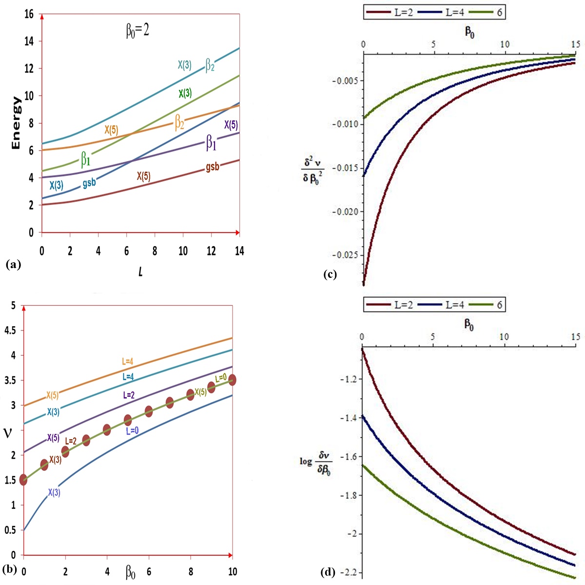
Figure 1: (a) Comparison in the energy levels of the $X(3)$ and the $X(5)$ models in ref.²⁷ at $\beta_{0}=2$ from the $gsb$ up to the $\beta_{2}$-excited states. (b) The variation of the critical order, $\nu^{X(5)}$ in ref.²⁷ as a function of $\beta_{0}$, is compared with $\nu^{X(3)}$ model at different angular momentum: $L=0,2$ and $L=4$. (c) The plots show the procedure from which the value of $\beta_{0}$ that corresponds to the minimum energy for each level is obtained. (d) The plot shows the rate at which the energy level changes with respect to $\beta_{0}$. This shows the non stationary property of $\beta_{0}$ in the description of critical point symmetries of isotopes.

holds in all the levels for both $X(3)$ and $X(5)$. This third remark is shown from the numerical values in the Table 2. The visual lines of the energies in the three states: the ground state and the $\beta$-excited states at $\beta_{0}=2$ are plotted and shown in Figure 1(a). In all the three states, for the same quantum levels, energy values for the $X(3)$ are higher than the energies of the $X(5)$.

Another significant remark deduced from the numerical values of $\nu$, tabulated in Table 1., is that $\nu^{X(5)}$ at $L=0$, correspond to $\nu^{X(3)}$ at $L=2$: the visual lines are seen in Figure 1(b) where the brown dotted line of $\nu^{X(3)}$ for different values of $\beta_{0}$ lies on the green line of $\nu^{X(5)}$ at $L=0$ for different values of $\beta_{0}$. The plot shows that no other lines of $\nu^{X(3)}$ coincides with the $\nu^{X(5)}$ again, they only increase with the increase in the angular momentum, $L$. Analytically, it can be stated that

$$\nu^{X(5)}(L=0)=\nu^{X(3)}(L=2)\quad\forall\quad\beta_{0}.$$ (27)

At, this juncture, it is wise to test for the stationary properties of the potential parameters as to know which of the parameters of the potential plays a major role in the dynamical symmetry of the model. It is expected that the n-derivatives of $\nu$ with respect to such parameter should be continuous in all the quantum levels. Having known the values of such parameter for certain isotopes, the numerical values for the spectra ratios, the $B(E2)$ and other nuclei collective signatures can be computed. Luckily enough in the present work, the potential employed is a one parameter dependent potential, it depends solely on the $\beta_{0}$. Therefore, the derivatives of $\nu$ with respect to the $\beta_{0}$ are taken and the continuous phenomenon and the lines of the $\frac{\delta^{2}\nu}{\delta\beta_{0}^{2}}$ and the $\frac{\delta\nu}{\delta\beta_{0}}$ at $L=2,4$ and at $L=6$ are respectively shown in Figures 1(c) and 1(d). Since the derivatives of $\nu$ with respect to $\beta_{0}$ is continuous, $\beta_{0}$ will yield to the variation procedure. Its forward or backward variation will provide some physical significance in the interpretation of the solution within the context of phase shape transition.

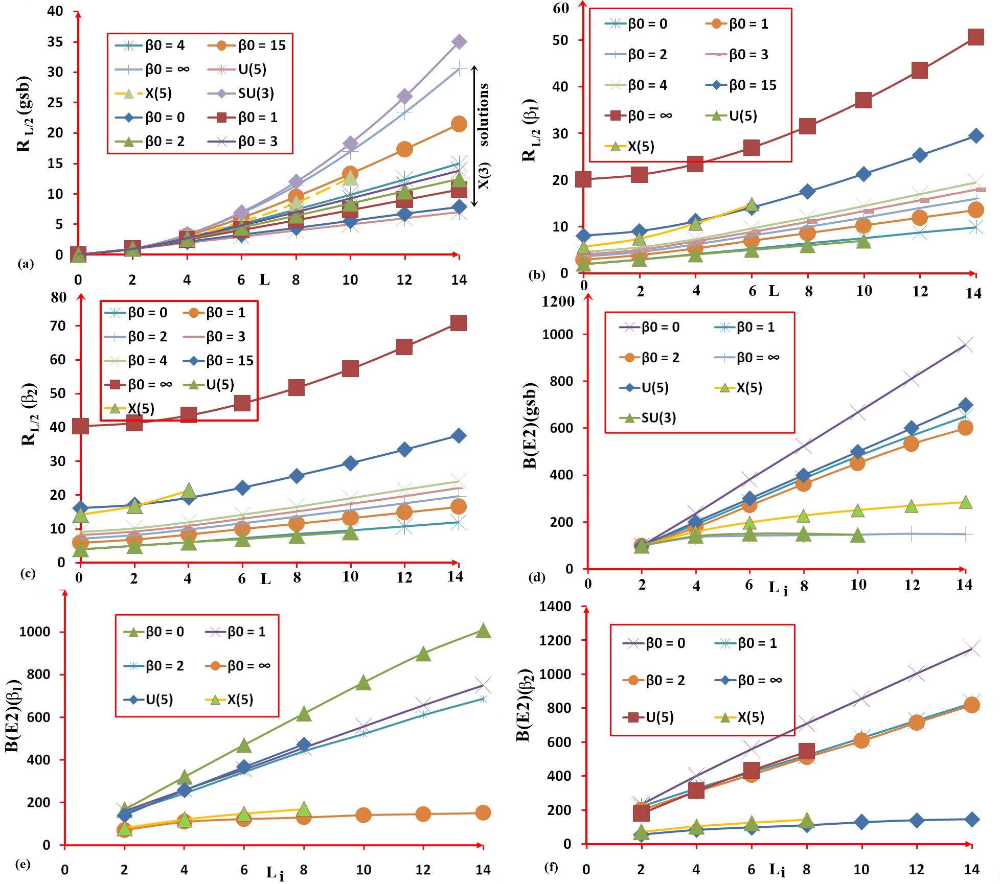
Figure 2: The spectra ratios of the present $X(3)$ model plotted against the angular momentum for different values of $\beta_{0}$ are placed for comparison with the $U(5)$ in ref.²⁹, the $X(5)$ in ref.²⁹ and the $SU(3)$ reported in ref.³⁰: the comparison in the ground state and the $\beta$-excited states are shown in (a), (b) and (c) respectively. (d) the the ground state (e) the $\beta_{1}$-excited states and (f) the $\beta_{2}$-excited states: of the $B(E2)$ plotted against the initial angular momentum and calculated for different values of $\beta_{0}$, are respectively compared with the $U(5)$ in ref.²⁹, the $X(5)$ in ref.²⁹ and the $SU(3)$ in ref.³⁰.

The spectra ratios of all the bands are normalized to the lowest excited energy level, $2_{1,0}$. The numerical values are computed and tabulated in Table 3. The ground state spectra ratios at different values of $\beta_{0}=0,1,2,3,4,5,15$ and $\beta_{0}=\infty$, are compared with the $X(5)$ in ref.²⁷ where the same potential has been used. The ground state spectra ratios and the $\beta$-excited spectra ratios at different values of $\beta_{0}=0,1,2,3,4,5,15$ and $\beta_{0}=\infty$, are compared with the $U(5)$ in ref.²⁹, the $X(5)$ model in ref.² and the $SU(3)$ reported in ref.³⁰. The spectra ratios at $\beta_{0}=0$ tend to the $U(5)$ vibrational limit while the spectra ratios at $\beta_{0}=\infty$ tend to the $SU(3)$ rotational limit. It can be seen, in the ground state where $SU(3)$ data are available, that $X(3)(\beta_{0}=\infty)$ and $X(5)(\beta_{0}=\infty)$, both with $R_{4/2}=3.296$ and marked with a ‘$\dagger$’ sign, approach $SU(3)$ whose ‘rotational’ excitation signature¹, $R_{4/2}=3.333$. The solutions from $\beta_{0}=0$ to $\beta_{0}=\infty$ spread over the $X(5)$. That is, the solutions move to the $X(5)$ as $\beta_{0}$ leaves zero and leave $X(5)$ going close to $SU(3)$ as $\beta_{0}$ goes to $\infty$, in a forward manner. The lines plotted in Figures 2(a), 2(b) and 2(c) visually show these comparisons in the ground state and the $\beta$-excited states respectively. In Figure 2(a), the width of the spread of the solutions over the $X(5)$ line is indicated by the arrow range line between $\beta_{0}=0$ and $\beta_{0}=\infty$. The ‘nature’ of critical point symmetry transitions for different isotopes, constrained to one-parameter potentials, can be investigated using a variational technique. This technique was introduced in the ref.³², used in ref.¹² to retrieve $U(5)$ and $O(6)$ in the ground state from the $E(5)$ within the domain of the one-parameter inverse square potential, it is also used in refs^12,14,26,27 and others. The forward variation of the ‘control parameter’, $\beta_{0}$, causes the nuclei transition from $X(5)$ to $SU(3)$. The nuclear shape phase region under investigation can predict the directions of the variation: whether forward variation or backward variation and also depends on the potential’s boundary conditions. The rate of change of the spectra ratios is maximized for each $L$ by using this technique. Each angular momentum is considered and treated separately in terms of the variation parameter, $\beta_{0}$, as the critical values of the spectra ratios are distinct. As shown in Table 4., the distinct value of $\beta_{0}$ that corresponds to each angular momentum obtained via $\beta_{0}$-optimization scheme^12,14,26,27 are labeled $\beta_{0,max}$. The calculated values of the $X(3)$ as a function of $\beta_{0,max}$, labeled $X(3)$-var are compared with $X(3)$-IW models in ref.⁸, $X(3)-\beta^{6}$ model found in ref.¹⁰ and $X(3)$-D model in ref.¹². There is a strong agreement between the present $X(3)$-var and $X(3)$-IW, the agreement is moderate between $X(3)-\beta^{6}$ model, $X(3)$-D model and the preset $X(3)$ model. In levels $0_{1,0}$ and $2_{1,0}$, $\beta_{0,max}=\beta_{0}$ because, any value of $\beta_{0}$ chosen will yield $0.000$ and $1.000$ for the calculations of $0_{1,0}$ and $2_{1,0}$ respectively. $\beta_{0,max}$ increases with increase in the angular momentum and its values are obtained at the points where the increase in $\beta_{0}$ becomes steep from the procedure $\dfrac{d}{d\beta_{0}}R_{L/2}|_{\beta_{0}=max}$, so that the rate of change of the spectra ratio is maximized. This procedure is carried out because, the shape formation of the critical points changes swiftly: such rapid change is seen just in the solutions tabulated in the third section of the Table 3., where the $U(5)$ vibrational limit properties of the solutions at $\beta_{0}=0$ rapidly change as $\beta_{0}>0$. From the numerical values of the spectra ratios computed at $\beta_{0}=0$, in Table 3., the relation

$$R_{L/2}(gsb)=2+R_{L/2}(\beta_{1})=4+R_{L/2}(\beta_{2}),$$ (28)

can be deduced. Regardless of the fractional part, this relation agrees with the $U(5)$ vibrational limit²⁹. This also suggests that the solutions at $\beta_{0}=0$ approach the $U(5)$ vibrational limit since the relation is not observed for spectra ratios at other values of $\beta_{0}>0$ . This is an observable effect or a signature from Eq.(26) while the effect of Eq.(24) is observed in the comparison of spectral ratios of $X(3)$ and $X(5)$ such that

$$R_{L/2}^{X(3)}(\beta_{0}=c+2)=R_{L/2}^{X(5)}(\beta_{0}=c);\quad c=0,1,2,...\quad.$$ (29)

The $B(E2)$ ratio is an additional structural signature for the quadrupole collective states that has been used in the searching for the shape phase change and for the critical point between two fixed symmetries. It is determined primarily from the normalized wave functions of Eq.(18) in Eq.(21). The numerical values of the $B(E2)$ transition rates of the present $X(3)$ model at $\beta_{0}=0,1,2$ and $\beta_{0}=\infty$, normalized to the $B(E2;2_{1,0}\rightarrow 0_{1,0})=100$ units are tabulated in the first section of Table 5. and are compared with the $U(5)$ in ref.²⁹, $X(5)$ in ref.² and $SU(3)$ reported in ref.³⁰. The solutions at $\beta_{0}=0$ lie close the $U(5)$ and go close to the axially symmetric prolate rotor, $SU(3)$, at $\beta_{0}=\infty$. As expected, the $B(E2)$ values decrease with the increase in the $\beta_{0}$ and the solutions spread over $X(5)$. The visual comparisons in the ground state and the $\beta$-excited states are respectively shown in Figures 2(d), 2(e) and 2(f). In the second section of Table 5., the $B(E2)$-var calculated in the present model, are compared with the $B(E2)$ solutions obtained from the infinite square well potential, $X(3)$-IW model, in ref⁸: the agreements between the two models in all the states are strong. This is because, the inverse square potential which can also be referred to as inverse square well has most properties of the infinite square well. Since each value of $\beta_{0,max}$ is distinct for each angular momentum, the values of $\beta_{0,max}^{(i)}$ and $\beta_{0,max}^{(f)}$ are the $\beta_{0,max}$ which correspond to the initial and final angular momenta considered in the transitions between the levels. They are obtained from the optimization procedure done for the spectra ratios recorded in the Table 4.

Before we discuss the experimental realization of this model, there is a need to show if the solutions presented and discussed before now, are dynamical symmetry. Now considering the interpretation of the Casten triangle⁴⁹ where the rotational excitation signature, $4_{1,0}$, of the isotopes mapped along $U(5)\rightarrow SU(3)$ region increase from $2.000$ to $3.333$, if either the model condition

$$U(5)\leq X(3)<SU(3),\quad\forall\quad\beta_{0},$$ (30)

is satisfied for both the spectra ratios and the $B(E2)$ or the numerical condition for the spectra ratios

$$\dfrac{L+2}{2}\leq R_{L+2/2_{1,0}}(X(3))<\dfrac{(L+2)(L+3)}{6},$$ (31)

is satisfied, then the solutions are said to be dynamical symmetry since the spectra ratios of the $U(5)$ is the same as the left hand side algorithm of Eq.(31) while $SU(3)$ obeys the right hand side algorithm of the same Eq.(31). The entire solutions from $\beta_{0}=0$ to $\beta_{0}=\infty$, in the Table 3. and Table 5., satisfy the conditions. $X(5)$ models also satisfy these conditions.

4.2 The experimental realization of the model

In the prediction of spectra ratios of the present $X(3)$ model, twelve best critical point isotopes, ¹⁰²Mo ref.³³, ^104-108Ru chain in refs^34-36, ^120-126Xe chain in refs^37-40, ¹⁴⁸Nd in ref.⁴¹, ^184-188Pt chain in refs^42-44 are considered for the experimental realization and for the numerical application. Since the model is meant to be compared with the $X(5)$ critical symmetry, $N=90$ isotones: ¹⁵⁰Nd in ref.⁴⁵, ¹⁵⁴Gd in ref.⁴⁶ and ¹⁵⁶Dy in ref.⁴⁷ known to be $X(5)$ candidates, are compared with the $X(3)$ theoretical model. In order to obtain the quality factor of the agreement, Eq.(14) is fitted with the experimental spectra and the free parameter of the potential, $\beta_{0}$, is determined for each isotope being considered. Having known the value of $\beta_{0}$ for each isotope, the quality factor which is the quantity that measures the agreement is

$$\sigma=\sqrt{\dfrac{\sum_{i}^{m}[(R_{s,L})^{Exp}_{i}-(R_{s,L})^{Theor}_{i}]^{2}}{m-1}},$$ (32)

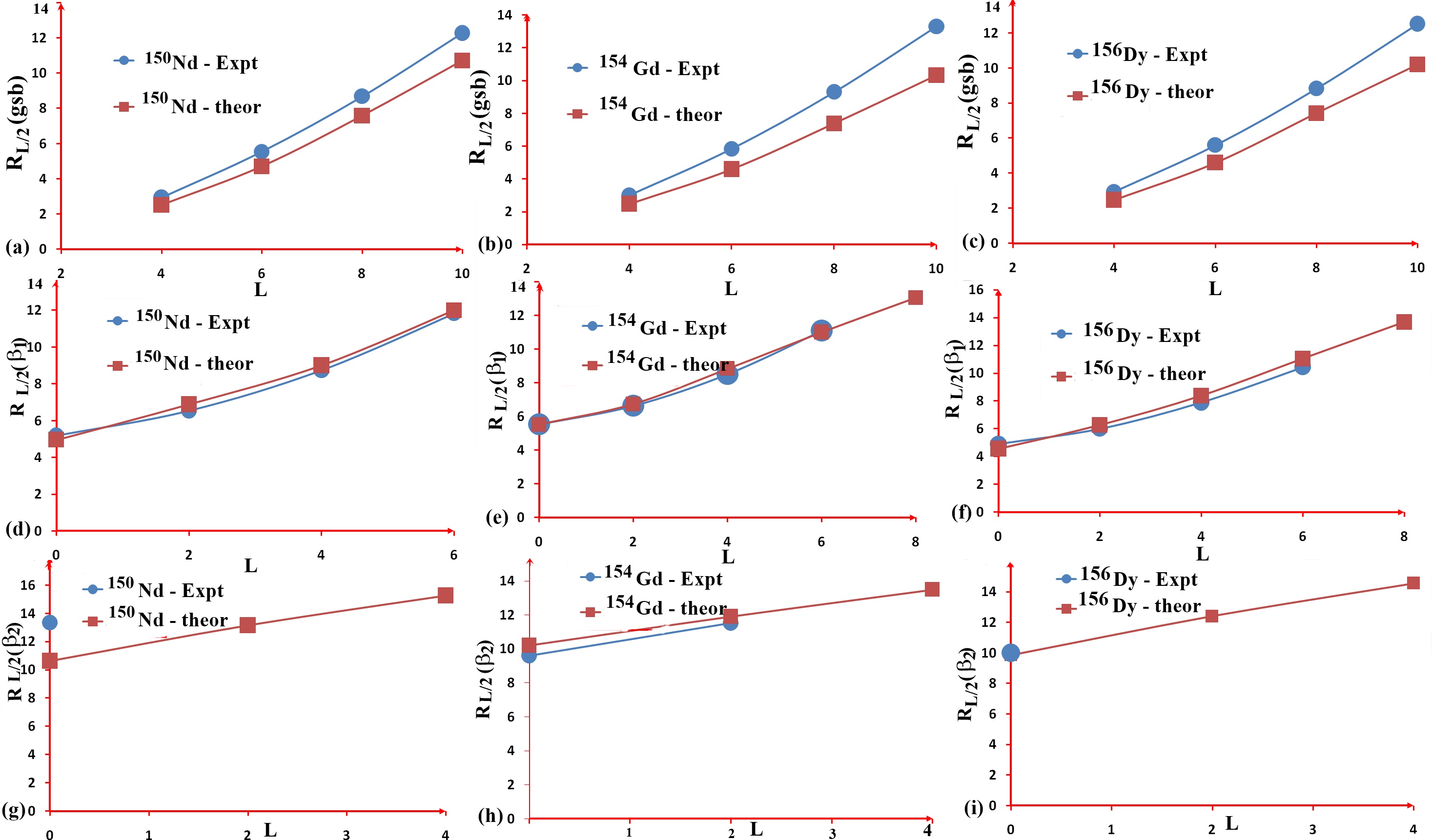
Figure 3: The visual comparison between the experimental data of the $X(5)$ candidates isotopes: ¹⁵⁰Nd in ref⁴⁵, ¹⁵⁴Gd in ref⁴⁶, ¹⁵⁶Dy in ref⁴⁷ and the spectra ratios of present $X(3)$ theoretical model in the ground state, the $\beta_{1}$-excited states and the $\beta_{2}$-excited states.

where $m$ is the number of available experimental states, $(R_{s,L})^{Exp}_{i}$ and $(R_{s,L})^{Theor}_{i}$ represent the experimental and the theoretical spectral ratios of the $i^{th}$ levels normalized to the ground state. These comparisons between the experimental spectra ratios and the theories are shown in the Table 6. While using the isotopes with the smallest quality factor such as ¹⁰⁸Ru, ¹⁰⁸Ru, ¹²²Xe, ¹²⁴Xe, ¹²⁶Xe to judge the agreement, it must be noted that isotopes with highest experimental states will yield smallest root mean square values. Regardless, except for ¹⁸⁸Pt with the highest quality factor, the quality factors for all the isotopes considered are in moderate agreement with the experimental data. This shows that the $X(3)$ inverse square model is a critical point symmetry model which presents the transition ‘around’ or near the vibrational $U(5)$ to prolate axially deformed shapes, $SU(3)$. In the same manner, ¹⁵⁰Nd, ¹⁵⁴Gd and ¹⁵⁶Dy are compared with the present $X(3)$ model in third section of Table 6. and the visual line in the ground state and the $\beta$-excited states are shown in Figure 3. There is no rational agreement in the ground states for the three isotopes, but an excellent prediction appears in the first $\beta$-excited state. This suggests that this present model can compensate the $X(5)$ models whose predictions are excellent in the ground states but moderately bad in the $\beta$-excited states. The ground states and the first $\beta$-excited states of the $B(E2)$ data for ¹⁰²Mo, ¹⁰⁴Ru, ¹⁰⁸Ru, ¹²⁰Xe, ¹²²Xe, ¹²⁴Xe, ¹⁴⁸Nd and one $X(5)$ candidate: ¹⁵²Sm isotope in ref.⁴⁸ are placed for comparison with the present $X(3)$ model. The $B(E2)$ values in Table 7. are not fitted, they are calculated with the values of $\beta_{0}$ recorded for the same isotopes from their fits on spectra. For ¹⁵²Sm, the $\beta_{0}=1.052$ and the quality the factor $\sigma=0.357$.

5 Conclusion

A new critical point symmetry model (CPSM) which is the $X(3)$ with the inverse square potential which presents the change from the region ‘around’ the $U(5)$ vibrational limit to prolate axially deformed shapes, $SU(3)$ limit in the frame work Bohr-Mottelson Hamiltonian is presented. The analytical form of the wave function and the one parameter-dependent energy spectra are obtained. The model is compared with the $X(5)$ model analytically to show the depth in the similarities and discrepancies in the context of the comparison, some new set of useful equations Eq.(24)- Eq.(31) are deduced. The model has proven sufficiently helpful in the description of $U(5)\rightarrow SU(3)$ region of the Casten triangle⁴⁹, since the solutions satisfy Eq.(30) and Eq.(31). The comparison of the present model with those found in the literature such as $X(3)$-IW model⁸, $X(3)-\beta^{6}$ model¹⁰ and $X(3)$-D model¹² is good. There is a strong agreement between the present $X(3)$-var and $X(3)$-IW model⁸ because the inverse square potential, its properties, are similar to those of infinite square well potential. The comparisons of the model with twelve best critical point isotopes, ¹⁰²Mo ref.³³, ^104-108Ru chain in refs^34-36, ^120-126Xe chain in refs^37-40, ¹⁴⁸Nd in ref.⁴¹, ^184-188Pt chain in refs^42-44 are moderate. An excellent agreement which appears in the first $\beta$-excited state in the comparison of the $X(3)$ via the inverse square potential with three $N=90$ isotones: ¹⁵⁰Nd in ref.⁴⁵, ¹⁵⁴Gd in ref.⁴⁶ and ¹⁵⁶Dy in ref.⁴⁷ known to be $X(5)$ candidates, suggests that this present model can compensate the $X(5)$ models whose predictions are very good in the ground states but performed poorly in the $\beta$-excited states.

Author Contribution:

KRA and KJO conceived, designed and drafted the work. KRA solved the differential equations, determined the wave functions, eigenvalues, spectra ratios, carried out variational technique to maximize the spectra ratios, and obtained the expression for the $B(E2)$ transition probabilities while KJO confirmed the correctness of the solutions and provided their numerical values. KRA plotted the graphs and LaTeX the work while KJO proof-read and approved the submission.

Data availability statement

The experimental data used for the experimental realization of our model are the published data: they are being cited and referenced accordingly. They are also available in the nuclear data sheet repository web link as of 2022: https://www.nndc. bnl.gov/nudat3/chartNuc.jsp.

Funding Information

No funding of any form is received for the course of this work.

References

[1] Iachello, F. Analytic Description of Critical Point Nuclei in a Spherical-Axially Deformed Shape Phase Transition. Phys. Rev. Lett. 87, 052502. doi: https://doi.org/10.1103/PhysRevLett.87.052502 (2001).

[2] Iachello, F. Dynamic Symmetries at the Critical Point. Phys. Rev. Lett. 85, 3580.
doi: https://doi.org/10.1103/PhysRevLett.85.3580 (2000).

[3] Iachello, F. and Arima, A. The Interacting Boson Approximation Model. Cambridge University Press, Cambridge.
doi: https://doi.org/10.1017/CBO9780511895517 (1987).

[4] Bohr, A. and Mottelson, B. The structure of Angular Momentum in Rapidly Rotating Nuclei. Nuclear Physics A., 354, (1-2), 303-31. doi: https://doi.org/10.1016/0375-9474(81)90604-7 (1981).

[5] Bohr, A. and Mottelson, B. Nuclear Structure Vol. I: Single-Particle Motion World Scientific Publishing Co. Pte. Ltd. Singapore. url: http://nuclphys.sinp.msu.ru/books/b/Bohr-Mottelson-I.pdf (1975).

[6] Bohr, A. The Coupling of Nuclear Surface Oscillations to the Motion of Individual Nucleons. Mat. Fys. Medd. Dan. Vid. Selsk. 26, 14. url: http://www.xuantianlinyu.com.cn/Jabref/RefPdf/Bohr1952pp.pdf(1952).

[7] Wilets, L. and Jean, M. Surface Oscillations in Even-Even Nuclei. Phys. Rev. C 102, 788.
doi: https://doi.org/10.1103/PhysRev.102.788 (1956).

[8] Bonatsos, D., Lenis, D., Petrellis, D., Terziev, P.A. and Yigitoglu, I. $X(3)$: an exactly separable $\gamma$-rigid version of the $X(5)$ critical point symmetry. Physics Letters B, 632, 238-242. doi: http://dx.doi.org/10.1016/j.physletb.2005.10.060 (2006).

[9] Budaca, R. Quartic oscillator potential in the $\gamma$-rigid regime of the collective geometrical model, Eur. Phys. J. A., 50, 87. doi: https://doi.org/10.1140/epja/i2014-14087-8 (2014).

[10] Budaca, R. Harmonic Oscillator Potential with a Sextic Anharmonicity in the Prolate $\gamma$-rigid Collective Geometrical Model. Physics Letters B, 739, 56-61. doi: http://dx.doi.org/10.1016/j.physletb.2014.10.031 (2014).

[11] Alimohammadi, M. and Hassanabadi, H. The $X(3)$ Model for the Modified Davidson Potential in a Variational Approach. International Journal of Modern Physics E. 26(9), 1750054. doi: http://dx.doi.org/10.1142/S0218301317500549 (2017).

[12] Yigitoglu, I. and Gokbulut, M. Bohr Hamiltonian for $\gamma=0^{0}$ with Davidson Potential. Eur. Phys. J. Plus, 132, 345. doi: http://dx.doi.org/10.1140/epjp/i2017-11609-3 (2017).

[13] McCutchan, E. A., Bonatsos, D., and Casten, R. F. Connecting the $X(5)-\beta^{2}$, $X(5)-\beta^{4}$, and $X(3)$ Models to the Shape-Phase Transition Region of the Interacting Boson Model. HNPS Advances in Nuclear Physics, 15, 118-127. doi: https://doi.org/10.12681/hnps.2628 (2020).

[14] Ajulo, K.R. and Oyewumi, K.J. Symmetry Solutions at $\gamma^{0}=\pi/6$ for Nuclei Transition Between $\gamma^{0}=0$ and $\gamma^{0}=\pi/3$ Via a Variational Procedure. Physica Scripta, 137(90). doi: https://doi.org/10.1088/1402-4896/ac76ed (2022).

[15] Davidson, P.M. Eigenfunctions for Calculating Electronic Vibrational Intensities. Proc. R. Soc. London, Ser. A., 135, 459. doi; https://doi.org/10.1098/rspa.1932.0045 (1932).

[16] Bonatsos et al., Exactly Separable Version of the Bohr Hamiltonian with the Davidson Potential. Phys. Rev. C 76, 064312. doi: https://doi.org/10.1103/PhysRevC.76.064312 (2007).

[17] Kratzer, A. Die ultraroten Rotationsspektren der Halogenwasserstoffe. Z. Physik 3, 307.
doi: https://doi.org/10.1007/BF01327754 (1920).

[18] Fortunato, L. Solutions of the Bohr Hamiltonian, a compendium. Eur. Phys. J. A., 26 (1), 1-30.
doi: https://doi.org/10.1140/epjad/i2005-07-115-8 (2005).

[19] Boztosun, I., Bonatsos, D. and Inci, I. Analytical Solutions of the Bohr Hamiltonian with the Morse Potential. Phys. Rev. C 77, 044302. doi: https://doi.org/10.1103/PhysRevC.77.044302 (2008).

[20] Inci, I., Bonatsos, D. and Boztosun, I. Electric Quadrupole Transitions of the Bohr Hamiltonian with the Morse Potential. Phys. Rev. C., 84, 024309. doi: https://doi.org/10.1103/PhysRevC.84.024309 (2011).

[21] Bohr, A. and Mottelson, B. Collective and Individual-Particle Aspects of Nuclear Structure. Mat-Fys. Medd. 27(16). 1-174. url: https://cds.cern.ch/record/213298/files/p1.pdf (1953).

[22] Bohr, A. and Mottelson, B. Nuclear Structure, Vol. II: Nuclear Deformations. W. A. Benjamin, Inc., Reading, Massachusetts, 748, 37-50. url: http://nuclphys.sinp.msu.ru/books/b/Bohr-Mottelson-I.pdf (1975).

[23] Davydov, A. S. and Chaban, A. A. Rotation-Vibration Interaction in Non-Axial Even Nuclei. Nucl. Phys. 20, 499-508. doi; https://doi.org/10.1016/0029-5582(60)90191-7 (1960).

[24] Bohr, A. The Coupling of Nuclear Surface Oscillations to the Motion of Individual Nucleons. Dan. Mat. Fys. Medd. 26(14). http://www.xuantianlinyu.com.cn/Jabref/RefPdf/Bohr1952pp.pdf (1952).

[25] Nikiforov, A.V. and Uvarov, V.B. Special Functions of Mathematical Physics. Birkhauser, Bassel.
doi: http://dx.doi.org/10.1007/978-1-4757-1595-8 (1988).

[26] Ajulo, K.R., Oyewumi, K.J., Oyun, O.S. and Ajibade, S.O. $U(5)$ and $O(6)$ Shape Phase Transitions Via $E(5)$ Inverse Square Potential Solutions. Eur. Phys. J. Plus, 136(500). doi: https://doi.org/10.1140/epjp/s13360-021-01451-7 (2021).

[27] Ajulo, K.R., Oyewumi, K.J., Oyun, O.S. and Ajibade, S.O. $X(5)$ Critical Symmetry with Inverse Square Potential Via a Variational Procedure. Eur. Phys. J. Plus 137(90). doi: https://doi.org/10.1140/epjp/s13360-021-02276-0 (2022).

[28] Casten, R.F. and Zamfir, N.V. Empirical Realization of a Critical Point Description in Atomic Nuclei. Phys. Rev. Lett. 87, 052503. doi: https://doi.org/10.1103/PhysRevLett.87.052503 (2001).

[29] Rowe, D.J., Turner, P.S. and Repka, J. Spherical Harmonics and Basic Coupling Coefficients for the Group $SO(5)$ in an $SO(3)$ Basis. J. Math. Phys. 45, 2761. doi: https://doi.org/10.1063/1.1763004 (2004).

[30] Bonatsos, D., Lenis, D., Minkov, N., Raychev, P.P. and Terziev. P. A. Extended $E(5)$ and $X(5)$ Symmetries: Series of Models Providing Parameter-Independent Predictions. Physics of Atomic Nuclei, 67(10), 1767-1775.
doi: https://doi.org/10.1134/1.1811176 (2004).

[31] Kotb. M. $U(5)-SU(3)$ Nuclear Shape Transition Within the Interacting Boson Model Applied to Dysprosium Isotopes. Physics of Particles and Nuclei Letters, 13(4), 451-459. doi: 10.1134/S1547477116040075 (2016).

[32] Bonatsos, D., Lenis, D., Minkov, N., Raychev, P.P. and Terziev. P.A. Ground State Bands of the $E(5)$ and $X(5)$ Critical Symmetries Obtained from Davidson Potentials Through a Variational Procedure. Physics Letters B, 584, 40-47.
doi:10.1016/j.physletb.2004.01.018 (2004).

[33] DE Frenne, D. Nucl. Data Sheets, 110(8), 1745-1915. doi: https://doi.org/10.1016/j.nds.2009.06.002 (2009).

[34] Blachot, J. Nucl. Data Sheets, 108(10), 2035-2172. doi: https://doi.org/10.1016/j.nds.2007.09.001 (2007).

[35] DE Frenne, D. and Negret, A. Nucl. Data Sheets, 109(4), 943-1102. doi: https://doi.org/10.1016/j.nds.2008.03.002 (2008).

[36] Blachot, J. Nucl. Data Sheets, 91(2), 135-296. doi: https://doi.org/10.1006/ndsh.2000.0017(2000).

[37] Kitao, K., Tendow, Y. and Hashizume, A. Nucl. Data Sheets, 96(2), 241-390. doi: https://doi.org/10.1006/ndsh.2002.0012 (2002).

[38] Tamura, T. Nucl. Data Sheets, 108(3), 455-632. doi: https://doi.org/10.1016/j.nds.2007.02.001(2007).

[39] Katakura, J. and Wu, Z.D. Nucl. Data Sheets, 109(7), 1655-1877. doi: https://doi.org/10.1016/j.nds.2008.06.001 (2008).

[40] Limura, H., Katakura, J. and Ohya, S. Nucl. Data Sheets, 180, 1-413. doi: https://doi.org/10.1016/j.nds.2022.02.001 (2022).

[41] Nica, N. Nucl. Data Sheets 117, 1-229. doi: https://doi.org/10.1016/j.nds.2014.02.001 (2014).

[42] Baglin, C.M. Nucl. Data Sheets, 111(2), 275-523. doi: https://doi.org/10.1016/j.nds.2010.01.001 (2010).

[43] Baglin, C.M. Nucl. Data Sheets, 99(9), 1-196. doi: https://doi.org/10.1006/ndsh.2003.0007 (2003).

[44] Singh, B. Nucl. Data Sheets, 95(2), 387-541. doi: https://doi.org/10.1006/ndsh.2002.0005 (2002).

[45] Basu, S.K. and Sonzogni, A.A. Nucl. Data Sheets, 114(4-5), 435-660. https://doi.org/10.1016/j.nds.2013.04.001 (2013).

[46] Reich, C.W. Nuclear data sheets for A = 154. Nucl. Data Sheets, 110, 2257. https://doi.org/10.1016/j.nds.2009.09.001 (2009).

[47] Reich, C.W. Nuclear Data Sheets for $A=156$ Nucl. Data Sheets, 113(11), 2537-2840.
https://doi.org/10.1016/j.nds.2012.10.003 (2012).

[48] Martin, M.J. Nucl. Data Sheets, 114(11), 1497-1847. https://doi.org/10.1016/j.nds.2013.11.001 (2013).

[49] R.F. Casten, Nuclear Structure from a Simple Perspective. Oxford University Press, Oxford.
url: https://radium.phys.uoa.gr/ebk/Casten-NuclearStructureFromASimplePerspective.pdf (1990).

Table 1: The comparison between the calculated values of the critical orders, $\nu$, for the $X(5)$ in Eq.(23) and $X(3)$ in Eq.(12) for both the even and the odd values of $\beta_{0}$.

$L$	$\beta_{0}=0$		$\beta_{0}=2$		$\beta_{0}=4$		$\beta_{0}=6$		$\beta_{0}=102$	$\beta_{0}=100$
	$X(3)$	$X(5)$	$X(3)$	$X(5)$	$X(3)$	$X(5)$	$X(3)$	$X(5)$	$X(3)$	$X(5)$
0	0.500	1.500	1.500	2.062	2.062	2.500	2.500	2.062	10.112	10.112
2	1.500	2.062	2.062	2.500	2.500	2.872	2.872	2.500	10.210	10.210
4	2.630	2.986	2.986	3.304	3.304	3.594	3.594	3.304	10.436	10.436
6	3.775	4.031	4.031	4.272	4.272	4.500	4.500	4.272	10.782	10.782
8	4.924	5.123	5.123	5.315	5.315	5.500	5.500	5.315	11.236	11.236
10	6.076	6.238	6.238	6.397	6.397	6.551	6.551	6.397	11.786	11.786
	$\beta_{0}=1$		$\beta_{0}=3$		$\beta_{0}=5$		$\beta_{0}=7$		$\beta_{0}=101$	$\beta_{0}=103$
0	1.118	1.803	1.803	2.291	2.291	2.693	2.693	3.041	10.062	10.259
2	1.803	2.291	2.291	2.693	2.693	3.041	3.041	3.354	10.161	10.356
4	2.814	3.149	3.149	3.452	3.452	3.731	3.731	3.990	10.388	10.579
6	3.905	4.153	4.153	4.387	4.387	4.610	4.610	4.823	10.735	10.920
8	5.025	5.220	5.220	5.408	5.408	5.590	5.590	5.766	11.191	11.369
10	6.158	6.318	6.318	6.474	6.474	6.627	6.627	6.776	11.747	11.913

Table 2: The ground state and the $\beta$ exited states energies in $\hbar=1$ unit, denoted by $n_{\beta}=0,s=1$; $n_{\beta}=1,s=2$; and $n_{\beta}=2,s=3$ respectively for the present $X(3)$ model and the $X(5)$ model in ref.²⁷.

	$\beta_{0}=2$	$\beta_{0}=2$	$\beta_{0}=3$	$\beta_{0}=3$	$\beta_{0}=4$	$\beta_{0}=4$	$\beta_{0}=15$	$\beta_{0}=15$
$L$					$n_{\beta}=0;s=1$
	$X(3)$	$X(5)$	$X(3)$	$X(5)$	$X(3)$	$X(5)$	$X(3)$	$X(5)$
0	2.500	2.031	2.803	2.146	3.062	2.250	4.905	3.077
2	3.062	2.250	3.291	2.346	3.500	2.436	5.153	3.194
4	3.986	2.652	4.149	2.726	4.304	2.797	5.682	3.445
6	5.031	3.136	5.153	3.194	5.272	3.250	6.408	3.795
8	6.123	3.658	6.220	3.704	6.315	3.750	7.265	4.212
10	7.238	4.198	7.318	4.237	7.397	4.276	8.205	4.671
					$n_{\beta}=1;s=2$
0	4.500	4.031	4.803	4.146	5.062	4.250	6.905	5.077
2	5.062	4.250	5.291	4.346	5.500	4.436	7.153	5.194
4	5.986	4.652	6.149	4.726	6.304	4.797	7.682	5.445
6	7.031	5.136	7.153	5.194	7.272	5.250	8.408	5.795
8	8.123	5.658	8.220	5.704	8.315	5.750	9.265	6.211
10	9.238	6.198	9.318	6.237	9.397	6.276	10.205	6.671
					$n_{\beta}=2;s=3$
0	6.500	6.031	6.803	6.146	7.062	6.250	8.905	7.077
2	7.062	6.250	7.291	6.346	7.500	6.436	9.153	7.194
4	7.986	6.652	8.149	6.726	8.304	6.797	9.682	7.445
6	9.031	7.136	9.153	7.194	9.272	7.250	10.408	7.795
8	10.123	7.658	10.220	7.704	10.315	7.750	11.265	8.211
10	11.238	8.198	11.318	8.237	11.397	8.276	12.205	8.671

Table 3: The ground state spectra ratios of the present $X(3)$ model, at different values of $\beta_{0}$, are compared with the $X(5)$ model in ref.²⁷ in the first and the second sections of the table. It can be seen that both $X(3)(\beta_{0}=\infty)$ and $X(5)(\beta_{0}=\infty)$, both with $4_{1,0}=3.296$ and marked by the ‘$\dagger$’ sign, approach $SU(3)$ whose ‘Rotational’ excitation signature¹, $4_{1,0}=3.333$. The third section compares the spectra ratios in the ground state and the $\beta$-excited states of the present model at different values of $\beta_{0}$ with the $U(5)$ in ref.²⁹, the $X(5)$ in ref.² and the $SU(3)$ reported in ref.³⁰. ‘-’ indicates the level where there is no data for comparison.

$L_{s,n_{\beta}}$	$\beta_{0}=0$	$\beta_{0}=0$	$\beta_{0}=2$	$\beta_{0}=2$	$\beta_{0}=4$	$\beta_{0}=4$	$\beta_{0}=\infty$	$\beta_{0}=\infty$
	$X(3)$	$X(5)$	$X(3)$	$X(5)$	$X(3)$	$X(5)$	$X(3)$	$X(5)$
$0_{1,0}$	0.000	0.000	0.000	0.000	0.000	0.000	0.000	0.000
$2_{1,0}$	1.000	1.000	1.000	1.000	1.000	1.000	1.000	1.000
$4_{1,0}$	2.130	2.646	2.646	2.834	2.834	2.938	†3.296	†3.296
$6_{1,0}$	3.275	4.507	4.507	5.042	5.042	5.372	6.806	6.808
$8_{1,0}$	4.424	6.453	6.453	7.421	7.421	8.508	11.413	11.423
$10_{1,0}$	5.576	8.438	8.438	9.887	9.887	11.881	16.991	17.013
$12_{1,0}$	6.728	10.445	10.445	12.404	12.404	15.686	23.409	23.450
$14_{1,0}$	7.882	12.465	12.465	14.951	14.951	19.740	30.544	30.611
	$\beta_{0}=1$	$\beta_{0}=1$	$\beta_{0}=3$	$\beta_{0}=3$	$\beta_{0}=5$	$\beta_{0}=5$	$\beta_{0}=15$	$\beta_{0}=15$
$0_{1,0}$	0.000	0.000	0.000	0.000	0.000	0.000	0.000	0.000
$2_{1,0}$	1.000	1.000	1.000	1.000	1.000	1.000	1.000	1.000
$4_{1,0}$	2.476	2.756	2.756	2.893	2.893	2.946	3.128	3.148
$6_{1,0}$	4.070	4.812	4.812	5.224	5.224	5.529	6.058	6.136
$8_{1,0}$	5.706	6.995	6.995	7.767	7.767	8.638	9.508	9.690
$10_{1,0}$	7.360	9.243	9.243	10.424	10.424	11.915	13.297	13.620
$12_{1,0}$	9.024	11.525	11.525	13.145	13.145	15.854	17.307	17.800
$14_{1,0}$	10.694	13.829	13.829	15.907	15.907	19.899	21.468	22.152
	$\beta_{0}=0$	$\beta_{0}=1$	$\beta_{0}=2$	$\beta_{0}=3$	$\beta_{0}=4$	$\beta_{0}=15$	$\beta_{0}=\infty$	$U(5)$	$X(5)$	$SU(3)$
$0_{1,0}$	0.000	0.000	0.000	0.000	0.000	0.000	0.000	0.000	0.000	0.000
$2_{1,0}$	1.000	1.000	1.000	1.000	1.000	1.000	1.000	1.000	1.000	1.000
$4_{1,0}$	2.130	2.476	2.646	2.756	2.834	3.128	†3.296	2.000	2.910	3.333
$6_{1,0}$	3.275	4.070	4.507	4.812	5.042	6.058	6.806	3.000	5.450	7.000
$8_{1,0}$	4.424	5.706	6.453	6.995	7.421	9.508	11.413	4.000	8.510	12.000
$10_{1,0}$	5.576	7.360	8.438	9.243	9.887	13.297	16.991	5.000	12.700	18.333
$12_{1,0}$	6.728	9.024	10.445	11.525	12.404	17.307	23.409	6.000	-	26.000
$14_{1,0}$	7.882	10.694	12.465	13.829	14.951	21.468	30.544	7.000	-	35.000
$0_{2,1}$	2.000	2.921	3.562	4.094	4.562	8.058	20.124	2.000	5.670	-
$2_{2,1}$	3.000	3.921	4.562	5.094	5.562	9.058	21.124	3.000	7.480	-
$4_{2,1}$	4.130	5.397	6.208	6.850	7.395	11.187	23.420	4.000	10.720	-
$6_{2,1}$	5.275	6.991	8.069	8.906	9.603	14.115	26.929	5.000	14.820	-
$8_{2,1}$	6.424	8.626	10.014	11.090	11.982	17.567	31.537	6.000	-	-
$10_{2,1}$	7.576	10.281	11.999	13.337	14.449	21.356	37.116	7.000	-	-
$12_{2,1}$	8.728	11.945	14.007	15.619	16.965	25.366	43.534	-	-	-
$14_{2,1}$	9.882	13.615	16.027	17.923	19.513	29.526	50.668	-	-	-
$0_{3,2}$	4.000	5.842	7.123	8.188	9.123	16.117	40.249	4.000	14.170	-
$2_{3,2}$	5.000	6.842	8.123	9.188	10.123	17.117	41.249	5.000	16.780	-
$4_{3,2}$	6.130	8.318	9.769	10.944	11.957	19.245	43.545	6.000	21.340	-
$6_{3,2}$	7.275	9.912	11.630	13.000	14.165	22.174	47.054	7.000	-	-
$8_{3,2}$	8.424	11.547	13.576	15.184	16.544	25.625	51.662	8.000	-	-
$10_{3,2}$	9.576	13.201	15.561	17.431	19.010	29.414	57.240	9.000	-	-
$12_{3,2}$	10.728	14.866	17.568	19.713	21.527	33.424	63.658	-	-	-
$14_{3,2}$	11.882	16.536	19.589	22.018	24.074	37.584	70.792	-	-	-

Table 4: The distinct value of the $\beta_{0}$ that corresponds to each angular momentum obtained via $\beta_{0}$-optimization scheme^{12,14,26,27,31} are labeled $\beta_{0,max}$. The calculated values of the $X(3)$ as a function of $\beta_{0,max}$, labeled $X(3)$-var are compared with $X(3)$-IW models in ref.⁸, $X(3)-\beta^{6}$ found in ref.¹⁰ and $X(3)$-D in ref.¹² [Note: IW denotes infinite square well potential; D denotes Davidson potential; var denotes variational method; ‘-’ indicates the level where there is no data for comparison.]

$L_{s,n_{\beta}}$	$\beta_{0,max}$	$X(3)$	$X(3)$	$X(3)$-D	$X(3)$	$L_{s,n_{\beta}}$	$\beta_{0,max}$	$X(3)$	$X(3)$	$X(3)$-D	$X(3)$
		var	IW	var	$\beta^{6}$			var	IW	var	$\beta^{6}$
$0_{1,0}$	$\beta_{0}$	0.000	0.000	0.000	0.000	$0_{3,2}$	2.524	7.701	7.650	-	6.013
$2_{1,0}$	$\beta_{0}$	1.000	1.000	1.000	1.000	$2_{3,2}$	4.497	10.553	10.560	-	7.925
$4_{1,0}$	0.844	2.440	2.440	2.570	2.343	$4_{3,2}$	6.523	14.088	14.190	-	10.193
$6_{1,0}$	1.576	4.244	4.230	4.620	3.905	$6_{3,2}$	8.567	18.172	18.220	-	12.606
$8_{1,0}$	2.033	6.383	6.350	7.130	5.654	$8_{3,2}$	10.438	22.613	22.620	-	15.141
$10_{1,0}$	2.143	8.666	8.780	10.050	7.571	$10_{3,2}$	11.932	25.999	-	-	17.791
$12_{1,0}$	2.695	11.421	11.520	13.470	9.642	$12_{3,2}$	13.011	28.928	-	-	20.551
$14_{1,0}$	3.643	14.573	14.570	17.300	-	$6_{2,1}$	5.213	10.327	10.290	-	7.968
$0_{2,1}$	0.815	2.703	2.870	-	2.556	$8_{2,1}$	6.098	13.493	13.570	-	10.141
$2_{2,1}$	2.101	4.619	4.830	-	4.080	$10_{2,1}$	6.855	16.908	17.180	-	12.449
$4_{2,1}$	3.729	7.255	7.370	-	5.941	$12_{2,1}$	8.106	21.009	21.140	-	14.884

Table 5: The first section of the table presents the $B(E2)$ transition rates of the present $X(3)$ model at $\beta_{0}=0,1,2$ and $\beta_{0}=\infty$, normalized to the $B(E2;2_{1,0}\rightarrow 0_{1,0})=100$ units are compared with the $U(5)$ in ref.²⁹, $X(5)$ in ref.² and $SU(3)$ reported in ref.³⁰. In the second section of the table, the $B(E2)$-var obtained are compared with the $B(E2)$ solutions obtained from the infinite square well potential, $X(3)$-IW, in ref⁸. ‘-’ indicates the level where there is no data for comparison.

$L_{s,n_{\beta}}^{(i)}$	$L_{s,n_{\beta}}^{(f)}$	$\beta_{0}=0$	$\beta_{0}=1$	$\beta_{0}=2$	$\beta_{0}=\infty$	$U(5)$	$X(5)$	$SU(3)$
$2_{1,0}$	$0_{1,0}$	100.000	100.000	100.000	100.000	100.000	100.000	100.000
$4_{1,0}$	$2_{1,0}$	207.941	190.935	178.005	136.126	200.000	159.890	140.650
$6_{1,0}$	$4_{1,0}$	328.565	286.006	270.996	141.873	300.000	198.220	150.540
$8_{1,0}$	$6_{1,0}$	472.664	384.599	369.090	143.368	400.000	227.600	150.970
$10_{1,0}$	$8_{1,0}$	589.862	486.036	469.991	146.653	500.000	250.850	146.190
$12_{1,0}$	$10_{1,0}$	693.722	587.658	559.744	152.134	600.000	269.730	-
$14_{1,0}$	$12_{1,0}$	802.769	690.364	671.484	159.359	700.000	285.420	-
$2_{2,1}$	$0_{2,1}$	156.813	160.292	152.428	69.929	140.000	79.520	-
$4_{2,1}$	$2_{2,1}$	310.619	260.000	243.186	109.222	257.140	120.020	-
$6_{2,1}$	$4_{2,1}$	463.542	355.240	343.376	121.324	366.670	146.750	-
$8_{2,1}$	$6_{2,1}$	591.111	456.792	439.962	130.219	472.730	169.310	-
$10_{2,1}$	$8_{2,1}$	718.669	557.317	542.129	139.999	-	-	-
$12_{2,1}$	$10_{2,1}$	876.003	656.999	639.677	145.282	-	-	-
$14_{2,1}$	$12_{2,1}$	1017.401	759.642	736.660	151.009	-	-	-
$2_{3,2}$	$0_{3,2}$	233.504	221.942	209.888	56.684	180.000	72.520	-
$4_{3,2}$	$2_{3,2}$	401.982	327.461	311.072	74.436	314.290	104.360	-
$6_{3,2}$	$4_{3,2}$	559.801	422.880	408.564	98.452	433.330	124.810	-
$8_{3,2}$	$6_{3,2}$	708.989	523.436	512.997	119.534	545.450	142.940	-
$10_{3,2}$	$8_{3,2}$	858.095	624.555	609.096	129.234	-	-	-
$12_{3,2}$	$10_{3,2}$	1003.933	727.909	715.990	140.274	-	-	-
$14_{3,2}$	$12_{3,2}$	1151.239	832.003	819.115	158.278	-	-	-
$L_{s,n_{\beta}}^{(i)}$	$L_{s,n_{\beta}}^{(f)}$	$\beta_{0,max}^{(i)}$	$\beta_{0,max}^{(f)}$	$B(E2)$	$X(3)$	$L_{s,n_{\beta}}^{(i)}$	$L_{s,n_{\beta}}^{(f)}$	$\beta_{0,max}^{(i)}$	$\beta_{0,max}^{(f)}$	$B(E2)$	$X(3)$
				-var	-IW					-var	-IW
$2_{1,0}$	$0_{1,0}$	$\beta_{0}$	$\beta_{0}$	100.000	100.00	$10_{2,1}$	$8_{2,1}$	6.855	6.098	242.026	242.40
$4_{1,0}$	$2_{1,0}$	0.844	$\beta_{0}$	189.495	189.90	$12_{2,1}$	$10_{2,1}$	8.106	6.855	268.543	265.10
$6_{1,0}$	$4_{1,0}$	1.576	0.844	250.995	248.90	$14_{2,1}$	$12_{2,1}$	9.441	8.106	281.32	-
$8_{1,0}$	$6_{1,0}$	2.033	1.576	293.038	291.40	$2_{3,2}$	$0_{3,2}$	4.497	2.524	72.090	73.50
$10_{1,0}$	$8_{1,0}$	2.143	2.033	324.599	323.80	$4_{3,2}$	$2_{3,2}$	6.523	4.497	118.990	120.50
$12_{1,0}$	$10_{1,0}$	2.695	2.143	350.710	349.50	$6_{3,2}$	$4_{3,2}$	8.567	6.523	154.892	154.20
$14_{1,0}$	$12_{1,0}$	3.643	2.695	371.992	370.70	$8_{3,2}$	$6_{3,2}$	10.438	8.567	183.019	181.20
$2_{2,1}$	$0_{2,1}$	2.011	0.815	78.922	80.60	$10_{3,2}$	$8_{3,2}$	11.932	10.438	202.222	-
$4_{2,1}$	$2_{2,1}$	3.729	2.101	139.471	140.10	$12_{3,2}$	$10_{3,2}$	13.011	11.932	218.753	-
$6_{2,1}$	$4_{2,1}$	5.213	3.729	181.730	182.40	$14_{3,2}$	$12_{3,2}$	14.629	13.011	229.986	-
$8_{2,1}$	$6_{2,1}$	6.098	5.213	213.899	215.50

Table 6: The numerical application of the spectra ratios of the present model is extended to twelve critical point isotopes: ¹⁰²Mo ref.³³, ^104-108Ru chain in ref.^34-36, ^120-126Xe chain in ref^37-40, ¹⁴⁸Nd in ref.⁴¹, ^184-188Pt chain in ref.^42-44 and also given to three $X(5)$ candidates: ¹⁵⁰Nd in ref.⁴⁵, ¹⁵⁴Gd in ref.⁴⁶ and ¹⁵⁶Dy in ref.⁴⁷ with the experimental data in the ground state, the first $\beta$-excited states and few data in the second $\beta$-excited states. The values of the $\beta_{0}$ and the quality factor, $\sigma$, used during the fittings are recorded. ‘-’ indicates the level where there is no data for comparison.

$L_{s,n_{\beta}}$	102Mo	102Mo	104Ru	104Ru	106Ru	106Ru	108Ru	108Ru	120Xe	120Xe	122Xe	122Xe
	Exp	Theor	Exp	Theor	Exp	Theor	Exp	Theor	Exp	Theor	Exp
$4_{1,0}$	2.510	2.566	2.480	2.468	2.660	2.662	2.750	2.623	2.470	2.522	2.500	2.571
$6_{1,0}$	4.480	4.483	4.350	4.299	4.800	4.805	5.120	5.102	4.330	4.263	4.430	4.500
$8_{1,0}$	6.810	6.703	6.480	6.488	7.310	7.199	8.020	7.999	6.510	6.361	6.690	6.759
$10_{1,0}$	9.410	8.989	8.690	8.702	10.020	9.920	11.310	11.495	8.900	8.497	9.180	9.216
$12_{1,0}$	-	11.498	-	11.878	-	12.334	-	12.879	-	10.362	-	11.985
$14_{1,0}$	-	13.302	-	14.522	-	15.073	-	15.591	-	12.640	-	14.759
$0_{2,1}$	2.350	3.009	-	2.569	3.670	3.678	-	4.462	2.820	3.000	3.470	3.492
$2_{2,1}$	3.860	4.301	4.230	4.233	-	5.127	-	5.902	3.950	4.203	4.510	4.608
$4_{2,1}$	-	6.289	5.810	5.921	-	7.443	-	8.285	5.310	5.899	-	6.792
$6_{2,1}$	-	8.691	-	8.009	-	10.001	-	11.099	-	7.958	-	9.172
$8_{2,1}$	-	11.319	-	11.101	-	12.519	-	14.532	-	10.739	-	11.829
$0_{3,2}$	-	7.437	-	6.589	-	8.388	-	10.099	-	6.664	-	7.722
$2_{3,2}$	-	9.000	-	8.202	-	10.200	-	11.811	-	8.007	-	9.402
$4_{3,2}$	-	11.009	-	10.341	-	12.049	-	12.972	-	10.229	-	11.538
$\beta_{0}$		1.464		0.963	-	2.121		1.830		1.221		1.494
$\sigma$		0.569		0.310	-	0.422		0.276		0.481		0.295
	124Xe	124Xe	126Xe	126Xe	148Nd	148Nd	184Pt	184Pt	186Pt	186Pt	188Pt	188Pt
$L_{s,n_{\beta}}$	Exp	Theor	Exp	Theor	Exp	Theor	Exp	Theor	Exp	Theor	Exp	Theor
$4_{1,0}$	2.480	2.498	2.420	2.463	2.490	2.500	2.670	2.721	2.560	2.567	2.530	2.890
$6_{1,0}$	4.370	4.418	4.210	4.291	4.240	4.187	4.900	5.001	4.580	4.399	4.460	4.503
$8_{1,0}$	6.580	6.596	6.270	6.325	6.150	6.007	7.550	7.679	7.010	6.768	6.710	6.666
$10_{1,0}$	8.960	8.726	8.640	8.382	8.190	7.986	10.470	10.585	9.700	8.863	9.180	8.969
$12_{1,0}$	-	11.998	-	10.479	-	9.769	-	12.807	-	11.999	-	11.378
$14_{1,0}$	-	15.079	-	12.681	-	11.246	-	15.367	-	14.875	-	14.242
$0_{2,1}$	3.580	3.402	3.380	3.201	3.040	3.082	3.020	3.546	2.460	2.798	3.010	3.209
$2_{2,1}$	4.600	4.498	4.320	4.241	3.880	4.006	5.180	5.452	4.170	4.381	4.200	4.397
$4_{2,1}$	5.690	6.289	5.250	5.862	5.320	5.589	7.570	7.943	6.380	6.599	-	6.583
$6_{2,1}$	-	8.564	-	7.828	7.120	7.411	11.040	11.157	8.360	8.581	-	8.603
$8_{2,1}$	-	11.900	-	10.062	-	9.752	-	14.601	-	12.007	-	12.100
$0_{3,2}$	-	7.334	-	6.759	-	6.249	-	10.122	-	7.389	-	7.603
$2_{3,2}$	-	8.888	-	8.009	-	7.442	-	11.900	-	8.942	-	9.162
$4_{3,2}$	-	10.022	-	9.287	-	9.051	-	12.998	-	10.208	-	10.441
$\beta_{0}$		1.101	-	0.949		1.111		2.639		1.469		4.950
$\sigma$		0.279	-	0.299		0.347		0.475		0.600		0.729
	150Nd	150Nd	154Gd	154Gd	156Dy	156Dy
$L_{s,n_{\beta}}$	Exp	Theor	Exp	Theor	Exp	Theor
$4_{1,0}$	2.930	2.501	3.010	2.483	2.930	2.466
$6_{1,0}$	5.530	4.696	5.830	4.392	5.590	4.593
$8_{1,0}$	8.680	7.576	9.300	7.375	8.820	7.410
$10_{1,0}$	12.280	10.711	13.300	10.324	12.520	9.699
$0_{2,1}$	5.190	4.958	5.530	5.521	4.900	4.561
$2_{2,1}$	6.530	6.891	6.630	6.742	6.010	6.268
$4_{2,1}$	8.740	9.010	8.510	8.839	7.900	8.371
$6_{2,1}$	11.830	12.004	11.100	11.008	10.430	11.033
$8_{2,1}$	-	13.857	-	13.062	-	13.682
$0_{3,2}$	(13.350)	10.633	9.600	10.202	10.000	9.863
$2_{3,2}$	-	13.148	11.52	11.899	-	12.393
$4_{3,2}$	-	15.261	-	13.484	-	14.151
$\beta_{0}$		4.284	-	0.956		0.998
$\sigma$		0.504	-	0.406		0.408

Table 7: The ground states and the first $\beta$-excited states of the $B(E2)$ experimental data for some critical points symmetry isotopes: ¹⁰²Mo, ¹⁰⁴Ru, ¹⁰⁸Ru, ¹²⁰Xe, ¹²²Xe, ¹²⁴Xe, ¹⁴⁸Nd and one X(5) candidate, ¹⁵²Sm in ref.⁴⁸ are compared with the present $X(3)$ model. Except for ¹⁵²Sm with the $\beta_{0}=1.052$ and the quality the factor $\sigma=0357$ which is fitted separately as done to the isotopes in Table 6., the values of $\beta_{0}$ used for calculating the $B(E2)$ of other isotopes are taken from Table 6. ‘-’ indicates the level where there is no data for comparison.

Isotope	$4_{1,0}\rightarrow 2_{1,0}$	$6_{1,0}\rightarrow 4_{1,0}$	$8_{1,0}\rightarrow 6_{1,0}$	$10_{1,0}\longrightarrow 8_{1,0}$	$0_{2,1}\longrightarrow 2_{1,0}$	$2_{2,1}\longrightarrow 2_{1,0}$
102Mo	120.000	-	-	-	-	-
	178.323	259.875	326.632	371.284	222.228	39.736
104Ru	143.000	-	-	-	-	-
	178.899	263.544	335.734	400.000	218.184	16.499
108Ru	165.000	-	-	-	-	-
	170.006	223.246	270.642	309.663	200.453	40.235
120Xe	116.000	117.000	96.000	91.000	-	-
	185.634	269.643	332.754	401.523	213.432	32.333
122Xe	146.000	141.000	103.000	154.000	-	-
	180.564	244.444	300.634	356.544	230.531	41.483
124Xe	117.000	152.000	114.000	36.000	-	-
	146.422	255.874	319.581	383.451	225.632	28.991
148Nd	162.000	176.000	169.000	-	54.000	25.000
	191.045	265.354	349.274	442.632	13.573	24.745
152Sm	144.000	166.000	202.000	217.000	23.000	4.000
	159.853	199.576	238.618	306.268	113.147	28.354
184Pt	165.000	178.000	213.000	244.000	-	-
	167.521	217.007	271.326	284.532	188.809	28.611