A low-mass hub-filament with double centre revealed in NGC2071-North

Abstract

We present the first analysis in NGC2071-North as a resolved hub-filament featuring a double centre. This $\sim 1.5\times 1.5$ parsec-scale filament hub contains $\sim$500 $M_{\odot}$. Seen from Planck, magnetic field lines may have facilitated the gathering of material at this isolated location. The energy balance analysis, supported by infalling gas signatures, reveal that these filaments are currently forming stars. Herschel 100 $\mu$m emission concentrates in the hub, at IRAS 05451+0037 and LkH$\alpha$ 316, and presents diffuse lobes and loops around them. We suggest that such a double centre could be formed, because the converging locations of filament pairs are offset, by 2.3′ ($0.27$ pc). This distance also matches the diameter of a hub-ring, seen in column density and molecular tracers, such as HCO⁺(1–0) and HCN(1–0), that may indicate a transition and the connection between the hub and the radiating filaments. We argue that all of the three components of the emission star LkH$\alpha$ 316 are in physical association. We find that a $\sim$0.06 pc-sized gas loop, attached to IRAS 05451+0037, can be seen at wavelengths all the way from Pan-STARRS-i to Herschel-100 $\mu$m. These observations suggest that both protostars at the double hub centre are interacting with the cloud material. In our ¹³CO data, we do not seem to find the outflow of this region that was identified in the 80s with much lower resolution.

1 Introduction

Thanks to recent space-based (e.g., Herschel) and sensitive ground-based (e.g., ALMA, EVLA) observations, much progress is being made on the early stages of star formation. This is being achieved by not only looking at the very peak of such sources, but also considering their near and far surroundings in the molecular clouds that are forming stars. In particular, many studies have shown that the cold material of molecular clouds is often organized in networks of filaments, whether these clouds are currently forming stars or not (e.g., Arzoumanian et al., 2011, 2019). Most of the clumps and cores are seen forming in these filaments (e.g., André et al., 2014; Könyves et al., 2015, 2020), the formation of which may be due to various mechanisms, invoking one or more of the turbulent-, gravitational-, and magnetic forces. Summaries on the origin of interstellar filaments can be found in André et al. (2014), Hacar et al. (2022), and Pineda et al. (2022).

Nearby Herschel filaments – up to $\sim$0.5 kpc distance – appear to be characterized by a narrow distribution of transverse half-power widths with a typical FWHM value of 0.1 pc (e.g., Arzoumanian et al., 2011, 2019; Koch & Rosolowsky, 2015). While there has been some debate about the reliability of this finding (cf., Panopoulou et al., 2022), tests performed on synthetic data suggest that published Herschel width measurements are not affected by significant biases, at least in the case of nearby, high-contrast filamentary structures (Arzoumanian et al., 2019; André et al., 2022).

The Orion B cloud complex at $d\sim 400$ pc (Menten et al., 2007; Lallement et al., 2014; Zucker et al., 2019) was studied by the Herschel Gould Belt survey (André et al., 2010). Here, Könyves et al. (2020) confirmed the physical existence of a transition in prestellar core formation efficiency (CFE) around a fiducial threshold of $A_{V}^{\rm bg}\sim 7$ mag in background visual extinction. This is similar to the trend observed with Herschel in other regions, such as the Aquila cloud (Könyves et al., 2015). Between $A_{V}^{\rm bg}\sim 5-10$ mag the CFE goes steeply from low to high, and the bulk of core and star formation is occurring above this threshold that had already been suspected earlier (e.g., Onishi et al., 1998; Johnstone et al., 2004; Kirk, H. et al., 2006). In the filamentary regions of NGC2023/24, NGC2068/71 (see Fig. 1 left) and the L1622 cometary cloud Könyves et al. (2020) found a total of 1768 starless cores ($\sim 28-45$% of which are gravitationally bound prestellar cores) and an additional 76 protostellar (Class 0-I) cores. In Orion B, the mass in prestellar cores above the mentioned threshold represents only a moderate fraction ($\sim 20$%); and $\sim$60–80% of the gravitationally bound cores are associated with filaments.

Interstellar filaments also play an important role in the formation of massive stars, where these dense elongated features are often organized in a “hub-filament” structure with converging arms (e.g., Myers, 2009; Peretto et al., 2013). Similar structures were called “junctions of filaments” by Schneider et al. (2012), who found that massive clusters more likely lie in the proximity of junctions of filaments in high column density regions, as Dale & Bonnell (2011) proposed from simulations.

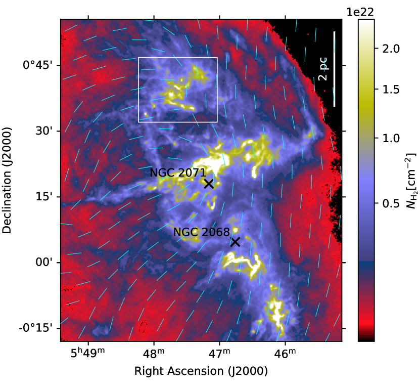
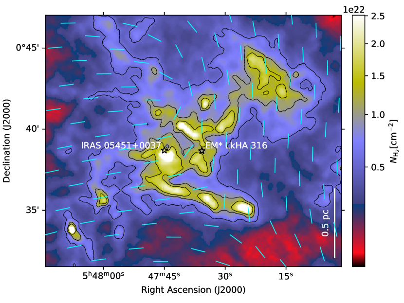
Figure 1: Left: Column density map of Orion B showing the region around NGC2071 (see Könyves et al., 2020). The white square outlines a $\sim 18\arcmin\times 15\arcmin$ field centred on RA=05:47:37.8, Dec=+00:39:16. The column density peak within this box, somewhat lower left from the centre, corresponds to $\sim 4\times 10^{22}$ cm^-2, where the dust filaments exhibit a multi-arm hub morhology. Right: Zoomed column density map on the filament hub, marking the locations of two embedded protostars. Black contours correspond to $N_{\rm H_{2}}$ = [5.5 $\times 10^{21}$, 9.7 $\times 10^{21}$, 1.4 $\times 10^{22}$] cm^-2, which are equivalent to $\sim$6, 10, and 15 magnitudes of visual extinction. The same contours are used in subsequent figures. In both panels Planck B-field-oriented vectors are overplotted in cyan on a 5′-scale (left), and 1.71′-scale (right).

Clumps with radiating multiple filaments can be seen in low-mass star-forming fields as well (e.g., in Pipe Nebula: Peretto et al., 2012). However, single filaments that do not cross each other (e.g., in Taurus: Palmeirim et al., 2013) appear to provide enough material to form solar-type stars. The hub-filament mode may be more typical, and its role may be more important, in regions of massive star formation, where the hub centre represents a deep potential well, able to accrete much more material from the surrounding filaments.

As for the role of the magnetic field ($B$-field) in the formation and evolution of such structures, a bimodal distribution of the relative orientations between the filaments and the mean magnetic field directions was found observationally, that is these relative orientations change from parallel to perpendicular with increasing (column) density. In other words, the relative orientations between the $B$-fields and the elongated structures were found to be mostly parallel in low-density filaments, and mostly perpendicular in dense filaments. These structures can be matched to the lower density “parallel” filaments and the high-density elongated hubs they are connected to in the hub-filament model by Myers (2009). Li et al. (2013) showed from observations that uniform (i.e., dynamically important) $B$-fields on larger scales can give rise to typical hub-filament cloud morphology. A strong interplay and the bimodality between interstellar $B$-fields and filaments were also shown by Planck Collaboration et al. (2016), and Alina et al. (2019), after these have been predicted by MHD simulations (Nakamura & Li, 2008; Soler et al., 2013; Chen et al., 2016; Soler & Hennebelle, 2017).

The region of interest of this work is a so far poorly studied sub-region north of NGC2071 that was named “NGC2071-North” (see Fig. 1 right) by Iwata et al. (1988). They made molecular observations in ¹²CO, ¹³CO, C¹⁸0(1–0), and NH₃ (1, 1) and (2, 2) lines, and followed up a CO outflow, discovered by Fukui et al. (1986). This relatively old ($t\sim 1.7\times 10^{5}$ yr) outflow shows a U-shape, and is apparently driven by IRAS 05451+0037. This was confirmed by Goldsmith et al. (1992) with 3 mm wavelength molecular observations. They argued that the molecular abundances in NGC2071-North (or NGC2071-N) have been significantly affected by this outflow and the presence of YSOs (young stellar objects). With this study we follow on from Gibb (2008), who also summarized the findings in NGC2071-N up to 2008.

As we mentioned above, cloud material may be channeled more efficiently through filaments into the seeds of star formation. However, newly-formed luminous sources can also significantly alter the geometry and composition of the surrounding material. While massive young stars can have dramatic effects on their neighbourhood by ionisation and major dynamical impact (HII regions, e.g., Tenorio-Tagle, 1982), winds and outflows of lower mass young stars can also sweep up gas and dust by injecting considerable mechanical energy into the ISM (cf., Snell, 1989). All of these feedback effects, which are an integral part of the star formation process, can trigger temperature and density changes in the surrounding matter.

Aspin & Reipurth (2000) performed optical CCD imaging around compact reflection nebulae and embedded IRAS sources in order to search for new Herbig-Haro (HH) jets and flows. They also identified a cluster of new HH objects associated with IRAS 05451+0037 and the nearby young star LkH$\alpha$ 316 in the centre of NGC2071-N.

Hillenbrand et al. (2012) detected strong emission-line features in the TiO and VO bands at the position of the optically-faint, flat-spectrum protostar IRAS 05451+0037 too, which suggests that it may be surrounded by dense and warm circumstellar gas.

Due to its relative isolation north of NGC2071 (see Fig. 1 left), this sub-region is still not well-studied. We present here the first analysis of NGC2071-N with high-resolution data sets of both the extended molecular material and the compact star-forming cores. It was hypothesized that it was once an elongated molecular clump along the E-W, SE-NW directions (Iwata et al., 1988; Goldsmith et al., 1992), and that NGC2071-North has now been refined into a ‘filamentary hub’ structure.

This paper is organized as follows. Section 2 provides details about the used data sets. In Section 3 we show distance results from Gaia EDR3 measurements, $Herschel$-derived properties, molecular line-derived properties, and we also estimate the energy balance based on energy densities and pressures. In Section 4 we discuss the large-scale magnetic field over NGC2071-N, we reason that star formation is on-going here, we discuss the double center, and revisit the existence of a CO outflow in the region. Finally, Section 5 presents our conclusions.

2 Observations and Data

2.1 Herschel data

In this study we used part of the SPIRE and PACS ‘parallel-mode’ Herschel Gould Belt survey (HGBS) observations of the Orion B complex region that includes NGC2071-N (see André et al., 2010). The details of the data reduction process are discussed by Könyves et al. (2020). In this work we used the SPIRE 250-$\mu$m data, calibrated in MJy sr^-1, on 3″-pixel scales. We also used the H₂ column density map that was created from the HGBS observations (see Könyves et al., 2020).

In addition, we used PACS-only mode 100-$\mu$m, and 160-$\mu$m data, also from the HGBS project (OBSIDs: 1342206054, 1342206055), observed on 08 October 2010 with a scanning speed of 20$\arcsec$s^-1 (as opposed to the parallel-mode’s 60$\arcsec$s^-1). They were reduced in the same way as the parallel-mode PACS observations (see Könyves et al., 2020).

2.2 IRAM 30 m observations

In the 2013 summer semester we carried out IRAM 30 m observations under project number 030–13. We used the EMIR receiver (Carter et al., 2012) at 3 mm to take fully-sampled C¹⁸O(1–0) and ¹³CO(1–0) maps simultaneously in a $\sim 108$ arcmin² region toward NGC2071-N. The on-the-fly mapping mode was used with position-switching. At 109.782 GHz, the 30 m telescope has a beam size of 23.6$\arcsec$ and the forward and main beam (MB) efficiencies ($F_{\rm eff}$ and $B_{\rm eff}$) are 95% and 79%, respectively. The backend used was the VESPA auto-correlator providing a frequency resolution of 20 kHz that corresponds to $\sim$ 0.055 km s^-1) in velocity resolution.

For the position-switching mode, the reference position was offsetted by $\sim$20′ from the map centre. The off position was selected from Herschel column density images, and we made sure that no significant CO emission is appearing there by observations in frequency-switching mode.

During the observations, calibration was performed every $\sim$30 minutes, and the telescope pointing was checked and adjusted every $\sim$2 hours. The pointing accuracy was found to be better than 3″. All of the data were reduced with the GILDAS/CLASS software package.

We smoothed the data spatially with a Gaussian function resulting in an effective beam size of 28$\arcsec$ ($\sim$0.05 pc at $\sim$400 pc). The 1$\sigma$ noise level of the final mosaicked data cube is $\sim$0.11 K in T_MB, at an effective angular resolution of 28$\arcsec$ and a velocity resolution of $\sim$0.1 km s^-1.

2.3 NRO 45 m observations

In 2015 we carried out observations on the 45-m telescope of the Nobeyama Radio Observatory toward a 0.14 square degree region in the Orion B cloud, including the densest portions of NGC2071-North, with the TZ receiver (Shimajiri et al., 2017). All molecular line data (HCN(1–0), H13CN(1–0), HCO+(1–0), and H13CO+(1–0)) were obtained simultaneously. At 86 GHz, the telescope has a beam size of 19.1″(HPBW) and a main beam efficiency of $\sim$50%. As a backend, we used the SAM45 spectrometer, which provides a bandwidth of 31 MHz and a frequency resolution of 7.63 kHz. The latter corresponds to a velocity resolution of $\sim$0.02 km s^-1 at 86 GHz. We applied spatial smoothing to the data with a Gaussian function resulting in an effective beam size of 30″. The 1-sigma noise level of the final data is $\sim$0.35 K in T_MB at an effective resolution of 30″and a velocity resolution of 0.1 km s^-1. More details of these observations and data reduction are described by Shimajiri et al. (2017).

Some of the image operations, such as $moment$ and $smooth$, were performed using the MIRIAD software package (Sault et al., 1995), for both the NRO and the IRAM observations.

2.4 Archival data

In order to trace and visualize NGC2071-North, in particular the central part of the hub, we have displayed and superimposed various data sets and catalogues within the interactive software Aladin sky atlas.

In addition to the above data sets, then we downloaded high-resolution short-wavelength SDSS, Pan-STARRS, and 2MASS images to further trace the interesting structures that we first caught in the 100 $\mu$m map (see Fig. 4).

SDSS images were retrieved from the SkyView Query Form which service resampled the data from the Sloan Digital Sky Survey. In this work we visualize SDSS data observed with the g, r, i colour filters.

2MASS J, H, K_s infrared images were also queried from NASA’s SkyView service.

Pan-STARRS is a system for wide-field astronomical imaging developed and operated by the Institute for Astronomy at the University of Hawaii. We downloaded DR2 data of the first part of the project to be completed through their Image Cutout Server Out of the five broadband filters (g, r, i, z, y), we used i, z, y.

To double-check the distance measurements in this region, we used Gaia Early Data Release 3 (Gaia EDR3) sources downloaded from the Gaia Archive.

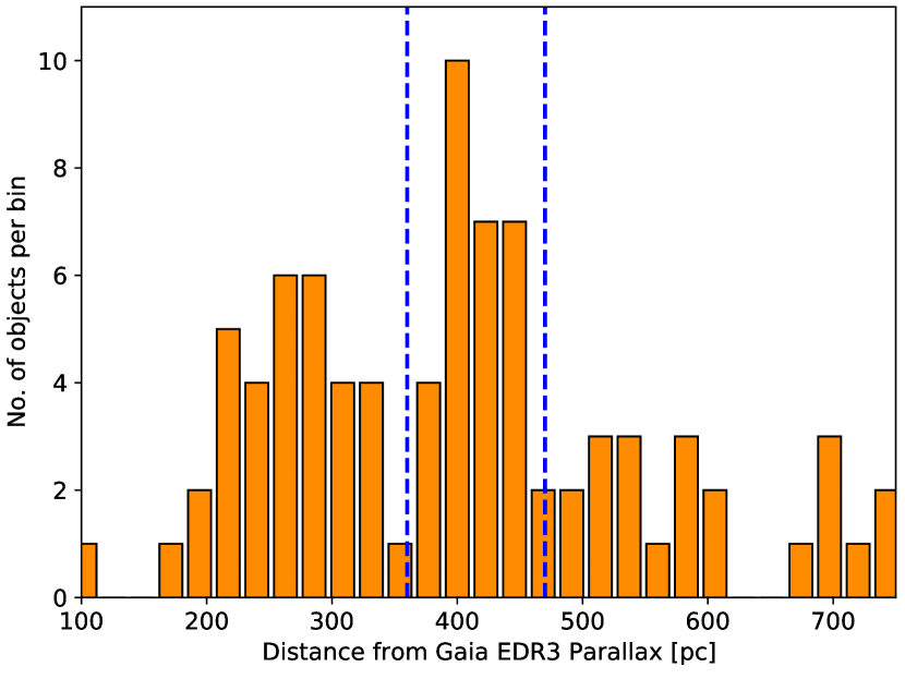
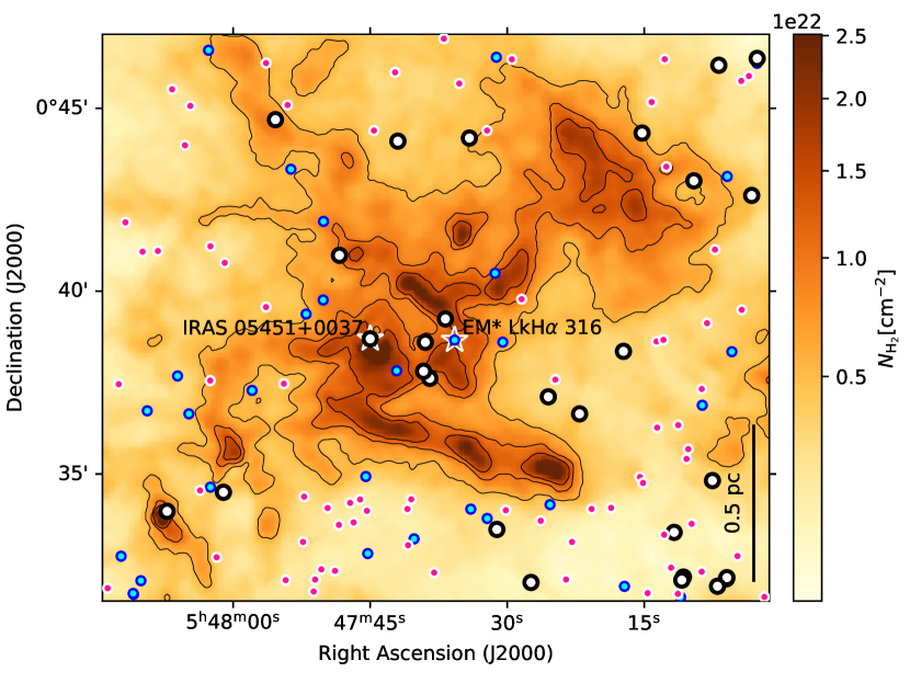
Figure 2: Left: Histogram of distances converted from Gaia EDR3 parallax measurements over the region shown in the right panel. Dashed blue lines mark the distances at 360 pc and 470 pc (see text for details). Right: Overlaid on column density, cyan/blue dots mark the Gaia measurement points at $d<360$ pc, white/black dots show the positions of $d=360-470$ pc measurements, which are a priori considered Orion B sources, and magenta/white dots mark the locations of Gaia EDR3 sources beyond 470 pc. Again, white stars mark the two named protostars.

3 Results and Analysis

3.1 Distance from Gaia EDR3 data

The most prominent features within Orion B are the Horsehead Nebula, the NGC 2023/24, NGC 2068/71 nebulae, as well as the Lynds 1622 (L1622) cometary cloud north-east of NGC2071-North (see Fig. 2 of Könyves et al., 2020). In the Lynds catalogue L1630 covers Orion B without L1622. As it was mentioned in Sect. 1, we consider $d\sim 400$ pc for the distance to most of the Orion B clouds (Anthony-Twarog, 1982; Menten et al., 2007; Gibb, 2008; Lallement et al., 2014; Schlafly et al., 2014; Zucker et al., 2019), while there is indication that the cometary, trunk-like features at and around L1622 may not be at this same distance. The alignment of the trunks and comets suggests that this northern part of Orion B interacts with the Barnard’s Loop (see Fig. 1 of Könyves et al., 2020). Thus, the L1622 region may also be at a closer distance ($\sim$170–180 pc), which is tentatively found for Barnard’s Loop by Bally (2008) and Lallement et al. (2014). However, its distance is still uncertain (see e.g., Ochsendorf et al., 2015, and references therein).

Revisiting Fig. 1 of Könyves et al. (2020) gave the idea to check the distances at NGC2071-N with available Gaia EDR3 data, as the H$\alpha$ shell of Barnard’s Loop seems to cut through Orion B between NGC2071 and L1622.

Gaia EDR3 measurements have been downloaded for the coverage shown in, for example, Fig. 1 right, from which we only exploited RA(J2000) and Dec(J2000) coordinates, parallax, and parallax errors. Distances in parsec from the parallax data (in arcseconds) have been converted with Astropy’s $to()$ unit conversion method (Greenfield et al., 2013). For the analysis, we ignored data points with negative parallax, as well as data where the parallax error was larger than half of the parallax value.

The histogram in the left-hand panel of Fig. 2 shows the distances for the region in the right-hand panel. A significant group of distances around 400 pc is apparent. However a very wide range of distances is found in this $\sim$18$\times$15 arcmin region. From the histogram, we set lower and upper distance limits around Orion B, at 360 pc and 470 pc, which seem to be reasonable choices, and they may also indicate a cloud depth, at NGC2071-N, of about 100 pc. The Gaia data points in these three distance ranges are plotted in Fig. 2 right. The cyan/blue dots mark the positions of Gaia measurements up to 360 pc, the white/black dots show the a priori Orion B sources between 360 pc and 470 pc, and the sources beyond 470 pc are marked with magenta/white dots. These latter ones most probably belong to the background, as they almost only appear where the cloud is more transparent (i.e., less column density). A group of white/black dots at around 400 pc is concentrated in the central portion of the hub and/or at higher column densities, which is reassuring. More also show up in the lower right corner that is in the direction of NGC2071. However the cyan/blue dots appear everywhere in the line of sight, and apparently the nebulous star LkH$\alpha$ 316, around the centre of NGC2071-N, also seems to lie closer to us than 360 pc.

Distances from EDR3 parallaxes of the two central objects, IRAS 05451+0037 and LkH$\alpha$ 316, gave us $d_{\rm IRAS}=383.4_{-14.2}^{+15.3}\,$pc, and $d_{\rm LkH\alpha}=300.6_{-36.5}^{+48.2}\,$pc, respectively, at which distances they may still belong to the same cloud.

After the above filtering of Gaia EDR3 measurement points, the distances range from $\sim$100 pc, to 6300 pc. They all are plotted in Fig. 2 right, while only those up to $\sim$800 pc are shown in the left-hand side histogram.

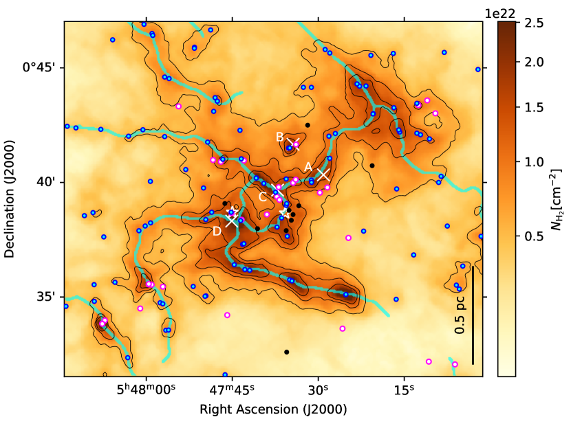
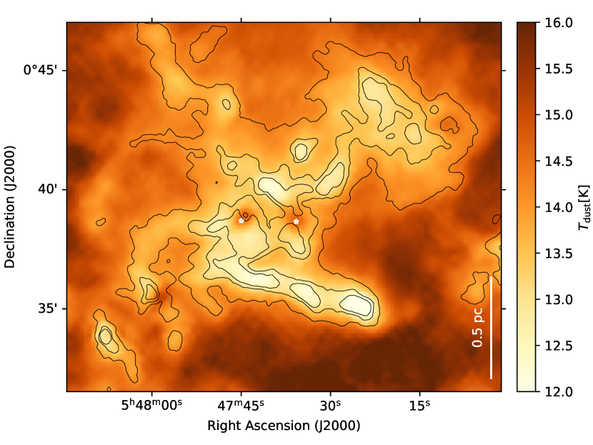
Figure 3: Left: Column density map of the NGC2071-N filament hub, with DisPerSE (Sousbie, 2011) filaments. Dense cores (bound prestellar and unbound starless) from Kirk et al. (2016a) and Könyves et al. (2020) are overplotted with cyan/blue dots. White/magenta dots mark YSOs/protostars from SIMBAD together with a few embedded protostars from Könyves et al. (2020). Black dots mark Herbig-Haro objects from SIMBAD. Four white crosses show the positions of NH₃(1, 1) cores defined by Iwata et al. (1988). Right: Dust temperature map of the same region. Maps and filaments are from Könyves et al. (2020). In both panels the left and right white stars (also protostars) mark the locations of IRAS 05451+0037 and LkH$\alpha$ 316, resp.

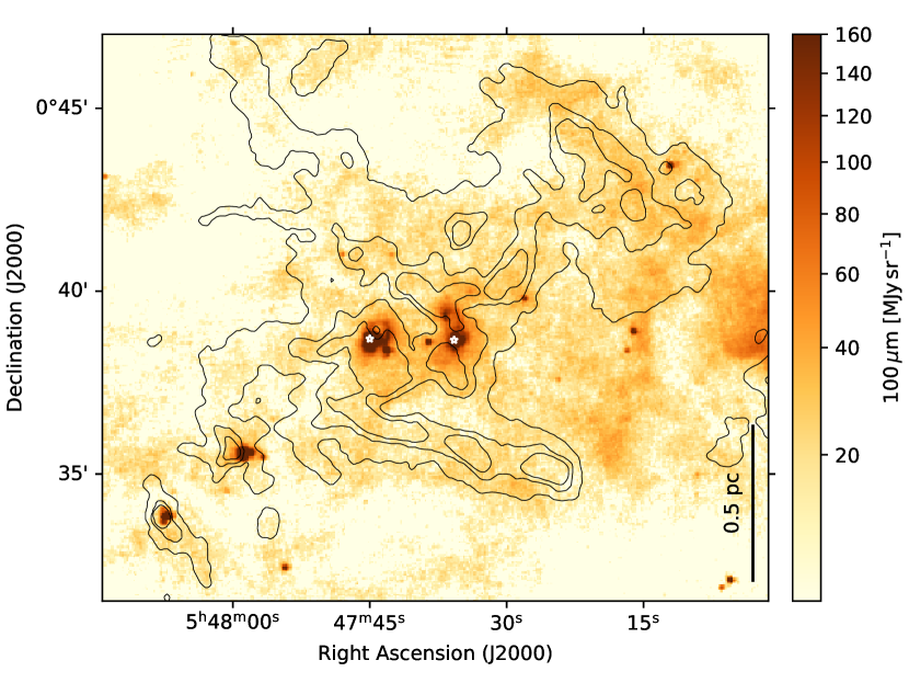
Figure 4: The same region as above in 100 $\mu$m emission. The left and right white stars mark the locations of IRAS 05451+0037 and LkH$\alpha$ 316, resp.

Table 1: Physical properties of 42 selected locations within 25″radius in NGC2071-N, shown in Fig. 5. See Sects. 3.2 and 3.4 for details. (1): Spot numbers, as in Fig. 5; (2) and (3): Right ascension and declination of spot centres; (4): Visual extinction calculated from median column density assuming $N_{\rm H_{2}}\,({\rm cm}^{-2})=0.94\times 10^{21}\,A_{\rm V}\,({\rm mag})$ (Bohlin et al., 1978); (5): Dust mass within these circles, no 20% error is included; (6) and (7): Dust temperature with stdev uncertainty; (8): average volume density; (9): gravitational energy density; (10): volume-averaged gravitational pressure; (11): Type of central object taken from the following studies: ¹ Könyves et al. (2020); ² Megeath et al. (2012); ³ Kirk et al. (2016b); ⁴ Gaia Collaboration (2018); ⁵ Cutri et al. (2003).

Spot no.	RA2000	Dec2000	$A_{\rm V}$	Mass	$T_{\rm dust}$	$n^{\rm ave}_{\rm H_{2}}$	$u_{\rm grav}$	$\overline{P}_{\rm G}/k_{\rm B}$	objtype
	(h m s)	(∘ ′ ″)	(mag)	($M_{\odot}$)	(K)	(104 cm-3)	(10-10 erg cm-3)	(105 K cm-3)
(1)	(2)	(3)	(4)	(5)	(6) $\pm$ (7)	(8)	(9)	(10)	(11)
1	05:47:37.00	+00:38:10.3	17.7	2.75	13.4   0.3	8.33	5.70	18.71	–
2	05:47:40.72	+00:38:16.4	12.7	2.06	13.3   0.1	6.23	3.19	10.50	–
3	05:47:44.50	+00:38:22.2	28.7	4.34	13.4   0.5	13.16	14.21	46.59	–
4	05:47:49.62	+00:38:22.9	14.2	2.18	12.8   0.1	6.61	3.58	11.75	prestellar core 1
5	05:47:55.55	+00:38:22.1	8.6	1.28	13.6   0.1	3.88	1.23	4.05	–
6	05:48:01.29	+00:37:53.8	8.2	1.29	13.7   0.1	3.93	1.26	4.12	prestellar core 1
7	05:48:01.75	+00:36:38.9	8.2	1.28	13.5   0.2	3.87	1.23	4.05	–
8	05:47:59.56	+00:35:34.3	12.9	1.91	14.1   0.6	5.80	2.77	9.02	protostellar core 1
9	05:47:56.12	+00:33:33.7	6.5	1.02	14.0   0.2	3.10	0.79	2.57	prestellar core 1
10	05:48:07.68	+00:33:49.9	13.6	2.46	13.1   0.2	7.46	4.56	14.97	protostellar core 1
11	05:47:42.98	+00:37:19.6	16.7	2.45	13.0   0.2	7.44	4.55	14.85	prestellar core 1
12	05:47:46.43	+00:36:39.6	17.3	2.68	12.6   0.2	8.12	5.41	17.77	–
13	05:47:41.96	+00:36:10.2	18.5	2.81	12.4   0.3	8.51	5.94	19.53	prestellar core 1
14	05:47:38.18	+00:35:57.0	13.2	2.05	12.9   0.2	6.22	3.18	10.39	–
15	05:47:34.59	+00:35:42.3	19.0	2.98	12.4   0.2	9.04	6.71	21.97	prestellar core 1
16	05:47:30.05	+00:35:21.4	12.1	1.89	13.0   0.1	5.72	2.69	8.84	–
17	05:47:25.18	+00:35:06.8	24.8	3.97	11.7   0.3	12.04	11.90	38.98	prestellar core 1
18	05:47:05.91	+00:35:31.3	6.6	1.01	14.1   0.2	3.07	0.77	2.52	starless core 1
19	05:47:40.36	+00:39:07.4	9.5	1.50	13.5   0.1	4.54	1.69	5.57	–
20	05:47:43.73	+00:39:26.2	12.1	1.82	13.5   0.3	5.53	2.51	8.19	–
21	05:47:35.51	+00:39:04.8	13.6	2.11	14.1   0.3	6.40	3.36	11.01	prestellar core 1
22	05:47:37.46	+00:39:34.5	18.8	2.98	13.2   0.4	9.03	6.69	21.97	prestellar core 1
23	05:47:40.82	+00:40:11.5	18.6	3.11	12.5   0.3	9.43	7.30	23.92	prestellar core 1
24	05:47:42.97	+00:40:57.4	12.0	1.86	13.3   0.1	5.65	2.62	8.56	YSO 2,4
25	05:47:46.66	+00:41:00.7	12.9	2.04	13.3   0.1	6.18	3.14	10.29	prestellar core 1
26	05:47:49.30	+00:41:45.7	9.4	1.44	13.6   0.1	4.38	1.57	5.13	prestellar core 1
27	05:47:53.00	+00:41:55.3	6.3	0.98	14.1   0.1	2.98	0.73	2.38	–
28	05:47:56.80	+00:42:00.1	5.9	0.90	14.2   0.1	2.73	0.61	2.00	dense core 3
29	05:48:03.10	+00:42:01.1	5.1	0.79	14.4   0.1	2.39	0.47	1.54	prestellar core 1
30	05:47:47.61	+00:43:32.8	9.6	1.48	13.4   0.1	4.49	1.66	5.42	prestellar core 1
31	05:47:56.03	+00:44:32.0	9.2	1.38	13.6   0.1	4.19	1.44	4.71	prestellar core 1
32	05:47:51.61	+00:45:51.3	6.8	1.07	14.2   0.1	3.24	0.86	2.83	starless core 1
33	05:47:58.87	+00:46:25.0	8.5	1.31	13.9   0.1	3.97	1.29	4.24	prestellar core 1
34	05:47:34.40	+00:39:59.1	15.0	2.31	13.2   0.1	7.02	4.04	13.2	YSO 2,5
35	05:47:31.17	+00:40:00.3	16.0	2.58	13.0   0.2	7.81	5.01	16.46	prestellar core 1
36	05:47:34.97	+00:41:30.5	14.7	2.39	12.9   0.2	7.23	4.30	14.13	prestellar core 1
37	05:47:28.00	+00:41:03.1	13.0	2.12	13.2   0.2	6.42	3.38	11.12	dense core 3
38	05:47:28.14	+00:42:01.1	10.9	1.66	13.5   0.1	5.03	2.07	6.82	prestellar core 1
39	05:47:24.34	+00:42:31.9	11.3	1.73	13.5   0.1	5.26	2.27	7.40	–
40	05:47:20.45	+00:42:59.5	16.0	2.50	13.1   0.1	7.58	4.72	15.46	prestellar core 1
41	05:47:15.96	+00:42:17.6	16.0	2.55	13.2   0.1	7.74	4.91	16.08	prestellar core 1
42	05:47:23.24	+00:44:18.0	17.5	2.69	12.9   0.1	8.16	5.46	17.90	prestellar core 1

3.2 Herschel properties of the hub-filament

The spectacular hub-filament structure of NGC2071-North, seen in Figures 1 & 2, is made up of high column density multi-arms, corresponding to equivalent visual extinctions of $A_{\rm V}\ga 5$. It is relatively isolated from NGC2071, thus this sub-region is still not much studied. It occupies a $\sim 1.5\times 1.5$ pc projected area at a distance of $\sim$ 400 pc, and it was identified as such a structure in HGBS images (Könyves et al., 2020).

We have studied the star-forming properties of these filaments in Könyves et al. (2020), where the dense core population of the whole Orion B cloud was discussed, also with respect of filaments (see Fig. 3 left). The mass of the NGC2071-North structure is found to be about 500 $M_{\odot}$ above $A_{V}\sim 5$ mag which is less than that of the Serpens-South filament hub; $\sim 750\,\mbox{$M_{\odot}$}$ in a $\sim 1\times 2$ pc region, most of which is even above $A_{V}\sim 10$ mag, assuming a distance of 260 pc (Könyves et al., 2015). On the other hand, the B59 filament hub in Pipe (Peretto et al., 2012) is at lower extinction, its mass above $A_{V}\sim 5$ is only $\sim 30\,\mbox{$M_{\odot}$}$ (covering the hub centre and one filament arm).

Dust temperatures, also derived from HGBS data, within the lowest contours in the column density map at 5.5 $\times 10^{21}$ cm^-2 are found to be $\sim$14 K or less (see Fig. 3 right). Within the densest portions (southern filament, clumps A, B, C, NW corner) the temperature drops below 13 K, while the direct surroundings (within $\sim$20″) of the two central protostars exhibit temperatures between 14 and 15 K.

The bound prestellar core masses are in the range of $\sim$0.2–10 $M_{\odot}$ with a median mass of $\sim$1 $M_{\odot}$, which would eventually collapse to low-mass stars. These sources are also among the overplotted ones in Fig. 3 left. The properties around them, together with further derived properties from Sect. 3.4, are listed in Table 1. In Fig. 3 left it is clear that most of the dense cores (cyan/blue dots) are located along filaments and elongated features. This tendency has been noted and discussed in several HGBS papers (e.g., André et al., 2014; Marsh et al., 2016; Benedettini et al., 2018; Ladjelate et al., 2020; Fiorellino et al., 2021), and this result does not depend significantly on the method of filament extraction (Könyves et al., 2020). This same figure panel also shows that YSOs and protostars (white/magenta dots) tend to appear at locations which are at the crossing points of filaments. For instance, at core C and D of Iwata et al. (1988) (identified from NH₃(1, 1) observations), which are at the junction of extracted filaments (in cyan). A similar effect on larger scales, that infrared clusters are found at the junction of filaments, has been found by several studies (Myers, 2009; Schneider et al., 2012; Peretto et al., 2013; Dewangan et al., 2015).

We also see diffuse and nebulous features at the apparent double-centre in the HGBS 100 $\mu$m map (see Fig. 4). At 100 $\mu$m the emission is concentrated in the central part of the filament hub, at IRAS 05451+0037 and EM* LkH$\alpha$ 316, and features diffuse lobes and loops. This kind of activity at 100 $\mu$m (and also at 70 $\mu$m) cannot be found in the neighbourhood; at least within $\sim$17′ to the south, and up to $\sim$1.8^∘ to the north, north-east (as far as L1622). For a better visualization of the central part of NGC2071-N, at various wavelengths, see Sect. 4.3.

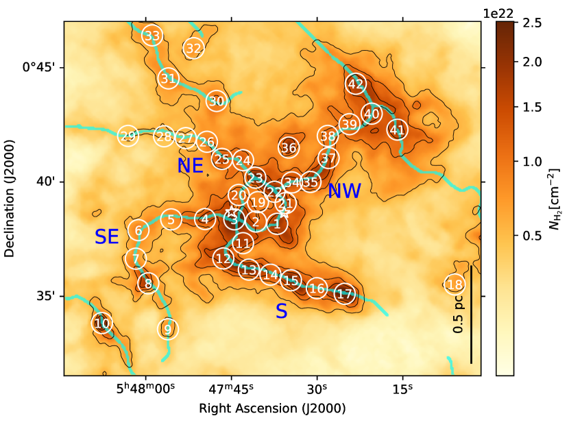
Figure 5: Column density map and filaments in NGC2071-N, as in Fig. 3 left. White numbered circles with 25″radius indicate the spots within which we estimated the energy balance (see Sects. 3.4 and 4.2, and Tables 1 and 2). Filament designations by their locations are also shown: southern (S); south-east (SE); north-east (NE); north-west (NW).

For the following calculations we mainly choose core positions, displayed in Fig. 3 left, that are sampling the filaments and the hub centre. Around them, we defined spots/circles (see Fig. 5) within which we then performed the measurements and calculations. For their sizes we defined a uniform 25″ (i.e, $\sim$0.05 pc) radius, knowing that the median FWHM size of the HGBS cores in this subregion is 0.05 pc. We may take the FHWM size as a radius, because 1) the column density profile of a critical Bonnor-Ebert sphere (e.g., Bonnor, 1956) with outer radius $R_{BE}$ is very well approximated by a Gaussian profile of FWHM $\sim R_{BE}$ (see in Könyves et al., 2015), and 2) for a Gaussian 2D circular distribution, $\sim$94% of the emission is contained within a circular aperture of radius FWHM (see also in Peretto et al., 2006). Thus, closely 100% of the flux and mass of the cores is contained in the –preferably non-overlapping– drawn circles in Fig. 5, within which we can also sample the molecular emission with independent beams. The two circles #1 and #3 were placed over column density peaks, and most of the rest of the positions correspond to starless, prestellar, protostellar dense cores, or YSOs. In these spheres we assume uniform densities.

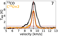
(a)

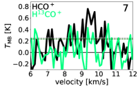
(b)

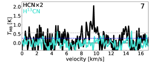
(c)

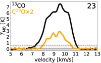
(d)

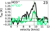
(e)

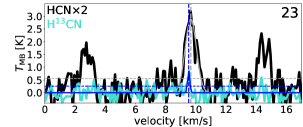
(f)

Figure 6: Spectra averaged over circles #7 & #23. All of them are $J=1\rightarrow 0$ transitions. When it is reasonable, a Gaussian fit and its peak position are also included. Dashed horizontal lines mark rms thresholds; grey for the black spectra, in colour for the overplotted spectra (6$\sigma$ rms level is indicated for the CO species, 3$\sigma$ for the HCX species). All of the avaraged spectra over the analysis circles (see Fig. 5) are included in Appendix A, when available. Derived properties from these molecular lines are listed in Table 2.

3.3 Molecular line data

Low- and high-density molecular line tracers of gas kinematics were also analysed in our NGC2071-North hub. ¹³CO(1–0) and C¹⁸O(1–0) observations were done with the IRAM 30 m telescope, HCN(1–0), H¹³CN(1–0) and HCO⁺(1–0), H¹³CO⁺(1–0) mapping were performed with the Nobeyama 45 m antenna.

Sample spectra of all these observed lines are displayed in Fig. 6. As example spot #7 has $A_{\rm V}\sim$8 mag, while the visual extinction is higher ($\sim$19 mag) in spot #23, which is also located at the junction of filaments in the central part of the hub. Among other properties, $A_{\rm V}$ values are listed for each analysis spot in Table 1. All of the avaraged spectra over these spots, where available, are included in Appendix A. When we find a reasonable Gaussian fit of the main component of the line, it is also overplotted on the spectra. The goodness of the fits has been evaluated with residual sum of squares, then we also eye-inspected the results.

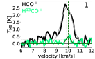
(a)

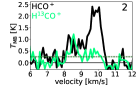
(b)

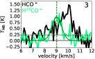
(c)

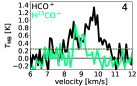
(d)

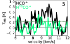
(e)

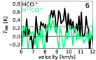
(f)

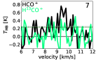
(g)

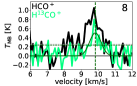
(h)

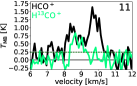
(i)

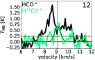
(j)

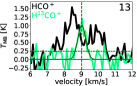
(k)

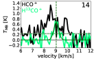
(l)

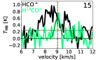
(m)

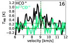
(n)

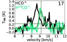
(o)

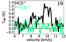
(p)

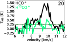
(q)

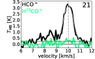
(r)

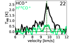
(s)

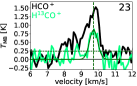
(t)

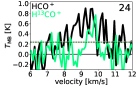
(u)

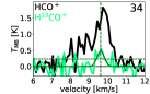
(v)

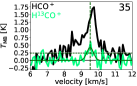
(w)

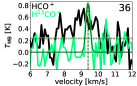
(x)

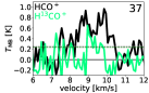
(y)

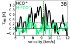
(z)

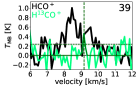
(aa)

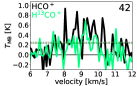
(ab)

Figure 10: HCO⁺(1–0) (black) and H¹³CO⁺(1–0) (light green) spectra averaged over the analysis spots where observed (see Fig. 5). When it is reasonable, a Gaussian fit and its peak position are also included. Dashed horizontal lines mark 3$\sigma$ rms thresholds; grey for the black spectra, green for the overplotted profiles. For details, see Sects. 3.3 and 3.4. Derived properties from these profiles are listed in Table 2.

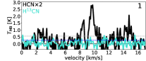
(a)

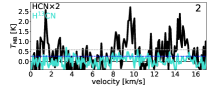
(b)

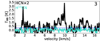
(c)

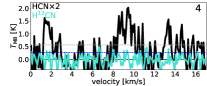
(d)

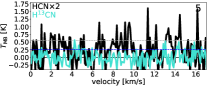
(e)

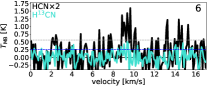
(f)

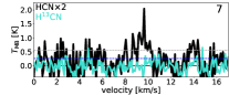
(g)

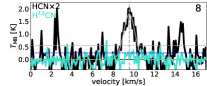
(h)

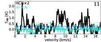
(i)

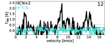
(j)

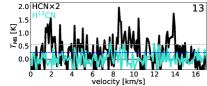
(k)

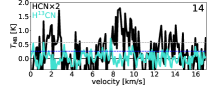
(l)

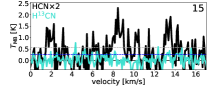
(m)

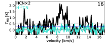
(n)

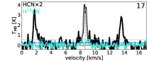
(o)

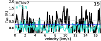
(p)

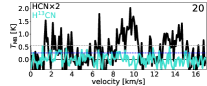
(q)

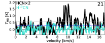
(r)

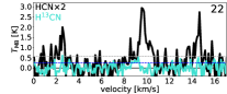
(s)

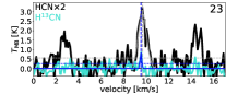
(t)

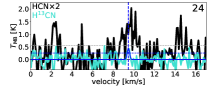
(u)

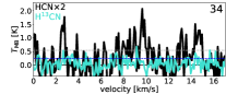
(v)

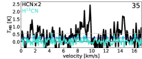
(w)

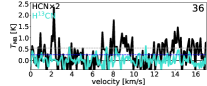
(x)

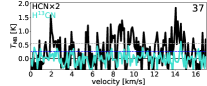
(y)

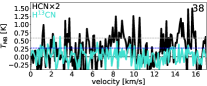
(z)

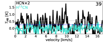
(aa)

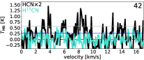
(ab)

Figure 11: HCN(1–0) (black) and H¹³CN(1–0) (cyan) spectra averaged over the analysis spots where observed (see Fig. 5). When it is reasonable, a Gaussian fit and its peak position are also included. Dashed horizontal lines mark 3$\sigma$ rms thresholds; grey for the black spectra, blue for the overplotted profiles. For details, see Sects. 3.3 and 3.4. Derived properties from these profiles are listed in Table 2.

Given the high column density values across NGC2071-N, we first evaluated the optical depth of the HCO⁺ and HCN lines with the help of their ¹³C-isotopes. We considered the same assumptions as Shimajiri et al. (2017) and used their Eq. 8 for deriving $\tau^{\rm HCO+}$ and $\tau^{\rm HCN}$. The peak intensity of the rare isotopic species we could fit only in limited cases (see Fig. 10 for H¹³CO⁺(1–0), and Fig. 11 for H¹³CN(1–0)). At the velocity position of the peak of the fit, we recorded the observed intensity (in $T_{\rm MB}$) of the averaged H¹³CO⁺ and H¹³CN lines, then that of the main species, HCO⁺ and HCN, at the same position. The resulting optical depths are listed in Table 2. The actual number results suggest that the HCO⁺ and HCN lines are optically thick, however $\tau^{\rm HCO+}$ at circle #8, and $\tau^{\rm HCN}$ at spot #24 may be upper limits. At the locations where the intensity of the main species is weaker than that of the rare species, most probably due to self-absorption, we indicate $\gg$1 as optical depth. In the rest of the cases, the emission of the rare species was not detected, or not well characterized by the fit. At the same time, based on the spectra, however noisy, we assume that the rare species, H¹³CO⁺ and H¹³CN, remain optically thin, or nearly so. Considering the critical densities of these rare $J=1\rightarrow 0$ lines at 10 K for local thermodynamic equilibrium (LTE), that is $n_{\rm crit}^{\rm H13CO+}=1.5\times 10^{5}$ cm^-3 and $n_{\rm crit}^{\rm H13CN}=2.0\times 10^{6}$ cm^-3 (Dhabal et al., 2018), our estimated volume densities are everywhere lower (see Table 1), with a median value of 6.23 $\times$ 10⁴ cm^-3.

High-density molecular tracers, especially when combining an optically thick and a thin line, can also indicate infalling gas, and thus global collapse of parts of the cloud (e.g., Myers et al., 1996; Evans, 1999; Schneider et al., 2010; Rygl et al., 2013; He et al., 2015; Traficante et al., 2017). This shows up in the thick tracer (i.e., HCO⁺) as a blue-red asymmetry, with brighter blue-shifted peak, whereas the thin line (H¹³CO⁺) peaks at the velocity of the self-absorption dip. Such configuration of the thin and thick lines we find in a couple of positions along the filaments (see Fig. 10) that we note with an upper index “c” in column 8 of Table 2. At these spots we have a strong hint that self-gravity plays a significant role that further analysis may confirm (see Sects. 3.4 and 4.2). These locations, except one, lie along the southern filament. Profiles of this shape also provide confirmation that the thick double peaks are not coming from two velocity components along the line of sight. Among these, the peaks of the thin lines (and the dips of the thick ones) are found at $V_{\rm LSR}\sim$9 km s^-1.

In addition to the presented line profiles and calculations, we are also providing the integrated intensity (moment 0) maps of the observed molecules in Appendix B, however they may be somewhat influenced by the optically thick conditions. In the case of the thin lines (H¹³CO⁺, H¹³CN), the integrated intensity of this region is much weaker and rather sparse.

3.4 Energy balance in NGC2071-North

From column density and optically thin molecular line data we have estimated gravitational and turbulent kinetic energy densities, as well as related gravitational and internal pressures in several spots within the region. These pressure terms contribute to the energy densities, nevertheless they are often equivalently used to evaluate the stability of clumps and clouds. We will separately probe the interplay between gravity and turbulence with the energy density and pressure properties, estimated with standard formulae and assumpsions.

Throughout the calculations we assume that the cores have spherical shape, uniform density, no contribution of external pressure or support of magnetic field, and no rotation either. In NGC2071-N there are no available polarisation observations (with comparable resolution to the above data) that we could derive magnetic energy densities, therefore we did not attempt to derive it from Planck measurements on 5′-scale, which would most probably characterize different phenomena.

The gravitational energy density was estimated from $u_{\rm grav}=4/5\pi G\rho^{2}R^{2}$ (see, e.g., Lyo et al., 2021), where $G$ is the gravitational constant, and $\rho=\mu m_{\rm H}n_{\rm H_{2}}$ is the uniform density for which the volume density we calculated from the $Herschel$ column density map of Könyves et al. (2020) (column (8) of Table 1). $R$ is the sphere radius (25″), $\mu=2.8$ is the mean molecular weight per H₂ molecule, and $m_{\rm H}$ is the hydrogen atom mass.

These calculations gave a mean value of $u_{\rm grav}=3.6\times 10^{-10}$ erg cm^-3 with a standard deviation of $2.8\times 10^{-10}$ erg cm^-3, for the whole range of results at the 42 locations in Fig. 5.

For a later comparison, the volume-averaged gravitational pressure can be estimated as $\overline{P}_{\rm G}/k_{\rm B}\approx 1.01a_{1}\langle\phi_{\rm G}\rangle M^{2}R^{-4}$, expressed by Bertoldi & McKee (1992), and used, for example, by Sadavoy et al. (2015). $k_{\rm B}$ is the Boltzmann constant, $a_{1}=1.3$ is a scaling factor that measures the effects of a nonuniform density distribution; our value is appropriate for a self-gravitating cloud. $\phi_{\rm G}$ is a scaling factor describing the cloud geometry; we consider $\phi_{\rm G}=1$ for perfect spheres. $M$ (in $M_{\odot}$) is the mass of the clumps (column (5) of Table 1), $R=0.048$ pc (used in pc) is the radius of our spots/spheres. We thus calculated the volume-averaged gravitational pressures that give a mean value of $\overline{P}_{\rm G}/k_{\rm B}=11.8\times 10^{5}$ K cm^-3 and a standard deviation of $9.3\times 10^{5}$ K cm^-3 for the whole range of results.

The individual values are listed in Table 1, along with additional physical properties. We assumed 20% error on the column densities, mass, then on the volume densities, energy densities, and pressures in order to avoid the propagation of the typical factor of about 2 systematic errors mainly due to the uncertainties in the dust opacity law.

The turbulent kinetic energy densities were calculated from $u_{\rm turb}=3/2\rho\sigma^{2}_{\rm NT}$, where $\sigma_{\rm NT}$ is the non-thermal component of the velocity dispersion. For this, first we converted the linewidths, as $\sigma=\Delta v/\sqrt{8~{}{\rm ln}2}$, that we estimated by Gaussian fitting to the observed profiles of H¹³CO⁺(1–0) and H¹³CN(1–0), where it was possible (see Sect. 3.3). Then, we separated the non-thermal component $\sigma_{\rm NT}$ using a similar relation to eqn. 6 of Dunham et al. (2011), and found that the observed velocity dispersions (or linewidths) are almost entirely due to non-thermal motions. These, we assume, may represent random turbulent motions (and infall motions), which are independent of the gas temperature. The resulting turbulent kinetic energy densities (for H¹³CO⁺, where it was possible to derive) yield a mean of $u_{\rm turb}^{\rm H13CO+}=3.23\times 10^{-10}$ erg cm^-3 with a high standard deviation of $3.20\times 10^{-10}$ erg cm^-3. From H¹³CN data, we could calculate $u_{\rm turb}^{\rm H13CN}$ only in two cases. See Figs. 10 and 11 for the fitted line profiles, and Table 2 for the derived line properties.

In comparison to the gravitational pressure, we estimate the internal pressure as well in the spots, where the quality of the H¹³CO⁺(1–0) and H¹³CN(1–0) spectra allowed us to derive turbulent kinetic energy densities too. The internal pressure can be approximated from the ideal gas law, as $P_{\rm int}/k_{\rm B}\approx n^{\rm ave}_{\rm H_{2}}\sigma^{2}_{\rm NT}$, where $n^{\rm ave}_{\rm H_{2}}$ is the average volume density (column (8) of Table 1), and $\sigma_{\rm NT}$ is the non-thermal part of the velocity dispersion, as above. In this or similar form the internal pressure has been calculated, for example, by Hatchell et al. (2005); Sadavoy et al. (2015); Pattle et al. (2015); Miville-Deschênes et al. (2017). The gravitational pressure estimates from H¹³CO⁺ can be summarized with a mean value of $P_{\rm int}/k_{\rm B}=5.4\times 10^{5}$ K cm^-3 with an as large standard deviation of $5.4\times 10^{5}$ K cm^-3.

Apart from the 20% uncertainties inherited from the column density measurements, we consider 1 standard deviation uncertainties on the measured median dust temperatures within the sampling spots. Along with the calculations of $\sigma_{\rm NT}$, $u_{\rm turb}$, and $P_{\rm int}$ we propagated the corresponding individual errors using the maximum error formula (see Tables 1 and 2, and Fig. 7 for the visualization of the uncertainties).

The left panel of Fig. 7 shows the estimated energy densities, where both $u_{\rm grav}$ and $u_{\rm turb}$ (latter from H¹³CO⁺ or H¹³CN) could be calculated. Such spots are denoted on the horizontal axis. In the right panel of Fig. 7, black and red data points display the volume-averaged gravitational pressure and internal pressure of these same locations, respectively, using the same molecular lines as in the left-hand panel. In both panels yellow stars indicate the positions where we observed possible infall signatures based on the blue-red asymmetry of the averaged HCO⁺ profiles (see Fig. 10). For a discussion involving Fig. 7, see Sect. 4.2.

Table 2: Physical properties of 42 selected locations within 25″radius in NGC2071-N, shown in Fig. 5. See Sects. 3.3 and 3.4 for details. (1): Spot numbers, as in Fig. 5; (2) $\pm$ (3), (4) $\pm$ (5), (6) $\pm$ (7), (9) $\pm$ (10), (15) $\pm$ (16), (18) $\pm$ (19): non-thermal velocity dispersion and uncertainties of the given (1–0) lines, ¹³CO, C¹⁸O, HCO⁺, H¹³CO⁺, HCN, H¹³CN, resp.; (8) and (17): optical depth of HCO⁺ and HCN, resp.; (11) $\pm$ (12), and (20) $\pm$ (21): turbulent kinetic energy densities and errors from H¹³CO⁺ and H¹³CN linewidths, resp.; (13) $\pm$ (14), and (22) $\pm$ (23): internal pressure and uncertainties at the latter locations. An upper index “c” in column (8) marks the spots where HCO⁺ speactra show infall signatures (see Fig. 10).

	13CO	C18O	HCO+		H13CO+			HCN		H13CN
Spot #	$\sigma_{\rm NT}^{\rm 13CO}$	$\sigma_{\rm NT}^{\rm C18O}$	$\sigma_{\rm NT}^{\rm HCO+}$	$\tau^{\rm HCO+}$	$\sigma_{\rm NT}^{\rm H13CO+}$	$u_{\rm turb}^{\rm H13CO+}$	$P^{\rm H13CO+}_{\rm int}/k_{\rm B}$	$\sigma_{\rm NT}^{\rm HCN}$	$\tau^{\rm HCN}$	$\sigma_{\rm NT}^{\rm H13CN}$	$u_{\rm turb}^{\rm H13CN}$	$P^{\rm H13CN}_{\rm int}/k_{\rm B}$
	(km s-1)	(km s-1)	(km s-1)	–	(km s-1)	(10-10 erg cm-3)	(105 K cm-3)	(km s-1)	–	(km s-1)	(10-10 erg cm-3)	(105 K cm-3)
(1)	(2) $\pm$ (3)	(4) $\pm$ (5)	(6) $\pm$ (7)	(8)	(9) $\pm$ (10)	(11) $\pm$ (12)	(13) $\pm$ (14)	(15) $\pm$ (16)	(17)	(18) $\pm$ (19)	(20) $\pm$ (21)	(22) $\pm$ (23)
1	–	–	0.48   0.03	11	0.19   0.07	2.09 $\pm$ 1.91	3.38 $\pm$ 3.10	–	–	–	–	–
2	–	–	–	–	–	–	–	–	–	–	–	–
3	–	–	–	$\gg$1	0.39   0.05	14.32 $\pm$ 6.47	24.38 $\pm$ 11.02	–	–	–	–	–
4	–	–	–	–	–	–	–	–	–	–	–	–
5	–	–	–	–	–	–	–	–	–	–	–	–
6	0.60   0.01	0.39   0.01	–	–	–	–	–	–	–	–	–	–
7	0.47   0.01	0.24   0.01	–	–	–	–	–	–	–	–	–	–
8	0.43   0.02	0.27   0.01	–	90	0.33   0.07	4.52 $\pm$ 2.92	7.64 $\pm$ 4.93	0.54   0.08	–	–	–	–
9	0.31   0.01	0.18   0.01	–	–	–	–	–	–	–	–	–	–
10	–	–	–	–	–	–	–	–	–	–	–	–
11	–	–	–	–	–	–	–	–	–	–	–	–
12	–	–	–	$\gg$1c	0.24   0.05	3.21 $\pm$ 2.01	5.33 $\pm$ 3.34	–	–	–	–	–
13	–	–	–	$\gg$1c	0.23   0.04	3.09 $\pm$ 1.60	5.12 $\pm$ 2.66	–	–	–	–	–
14	–	–	–	$\gg$1c	0.21   0.05	1.88 $\pm$ 1.28	3.08 $\pm$ 2.10	–	–	–	–	–
15	–	–	–	$\gg$1c	0.22   0.06	3.09 $\pm$ 2.21	5.11 $\pm$ 3.66	–	–	–	–	–
16	–	–	–	$\gg$1c	0.21   0.05	1.77 $\pm$ 1.20	2.91 $\pm$ 1.97	–	–	–	–	–
17	–	–	–	$\gg$1c	0.24   0.04	5.05 $\pm$ 2.72	8.45 $\pm$ 4.55	0.23   0.03	–	–	–	–
18	–	–	–	–	–	–	–	–	–	–	–	–
19	–	–	–	–	–	–	–	–	–	–	–	–
20	–	–	–	–	–	–	–	–	–	–	–	–
21	–	–	0.43   0.02	–	–	–	–	–	–	–	–	–
22	–	–	–	14	0.26   0.06	4.23 $\pm$ 2.97	7.07 $\pm$ 4.97	–	–	–	–	–
23	–	–	–	59	0.24   0.04	3.76 $\pm$ 2.02	6.27 $\pm$ 3.36	0.37   0.04	61	0.07   0.02	0.29 $\pm$ 0.23	0.25 $\pm$ 0.20
24	–	–	–	–	–	–	–	–	89	0.11   0.06	0.46 $\pm$ 0.45	0.64 $\pm$ 0.60
25	0.77   0.02	0.39   0.01	–	–	–	–	–	–	–	–	–	–
26	0.66   0.01	0.31   0.01	–	–	–	–	–	–	–	–	–	–
27	0.65   0.02	0.27   0.01	–	–	–	–	–	–	–	–	–	–
28	–	–	–	–	–	–	–	–	–	–	–	–
29	–	–	–	–	–	–	–	–	–	–	–	–
30	–	–	–	–	–	–	–	–	–	–	–	–
31	–	–	–	–	–	–	–	–	–	–	–	–
32	–	–	–	–	–	–	–	–	–	–	–	–
33	–	–	–	–	–	–	–	–	–	–	–	–
34	–	–	–	30	0.19   0.06	1.73 $\pm$ 1.48	2.81 $\pm$ 2.40	–	–	–	–	–
35	–	–	–	34	0.19   0.07	2.03 $\pm$ 1.86	3.30 $\pm$ 3.03	–	–	–	–	–
36	–	–	–	$\gg$1	0.11   0.03	0.62 $\pm$ 0.42	0.88 $\pm$ 0.60	–	–	–	–	–
37	–	–	–	–	–	–	–	–	–	–	–	–
38	–	–	–	$\gg$1	0.08   0.03	0.23 $\pm$ 0.22	0.26 $\pm$ 0.24	–	–	–	–	–
39	–	–	–	$\gg$1c	0.05   0.03	0.11 $\pm$ 0.10	0.05 $\pm$ 0.04	–	–	–	–	–
40	–	–	–	–	–	–	–	–	–	–	–	–
41	–	–	–	–	–	–	–	–	–	–	–	–
42	–	–	–	–	–	–	–	–	–	–	–	–

4 Discussion

4.1 Large-scale magnetic field pattern

Revisiting the panels of Fig. 1, we can see the large-scale structure of the POS magnetic field that was discussed in Soler (2019) for the whole Orion A and B clouds too. What shows up in Fig. 1 right is that the POS magnetic field (on the scale of 1/3 of the 5′ Planck beam) is largely horizontal in the eastern part, and vertical in the western part, as it would turn and change orientation across the hub.

Comparing Fig. 1 left with Fig. 4 of Soler (2019) and Fig. 8 of Tahani et al. (2018), we can see that there is a magnetic loop structure apparently starting or ending at NGC2071, extending up to NGC2071-N, while the B-field lines run mostly along the right ascension lines in the western side of all the clouds shown in Fig. 1 left.

Providing that the magnetic field is carrying material, a significant change in the B-field orientation (i.e., from horizontal to perpendicular) may be an efficient configuration for deposing and gathering gas and dust, which could also explain the location of this relatively small and isolated cloud. Not discussing here other physical forces, indeed it can be seen in the ISM that the B-field shows a bend and turns at high-density (elongated) molecular clouds, such as Orion A, Perseus, unlike in Musca and the Chamaeleon, for example. See these maps of Planck POS magnetic field and column density in Soler (2019).

We note that in the case of Orion A, such a simple visualization helped Tahani et al. (2018) to conclude that a bow-shaped magnetic field is surrounding that filament.

However, how the large-scale magnetic field is cascading down, and most likely affecting the morphology of the centre of the hub, is not yet known.

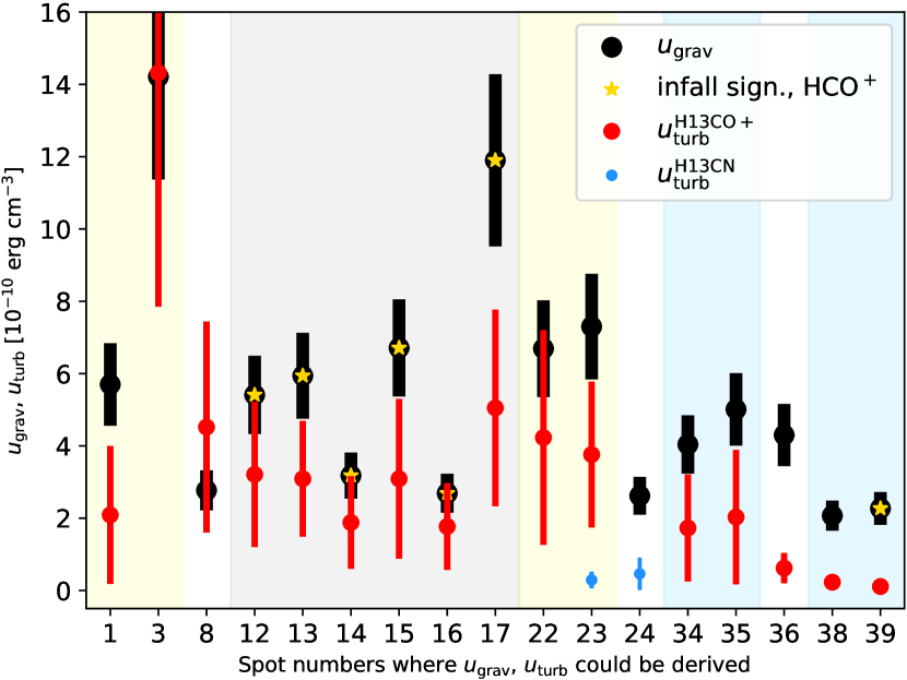
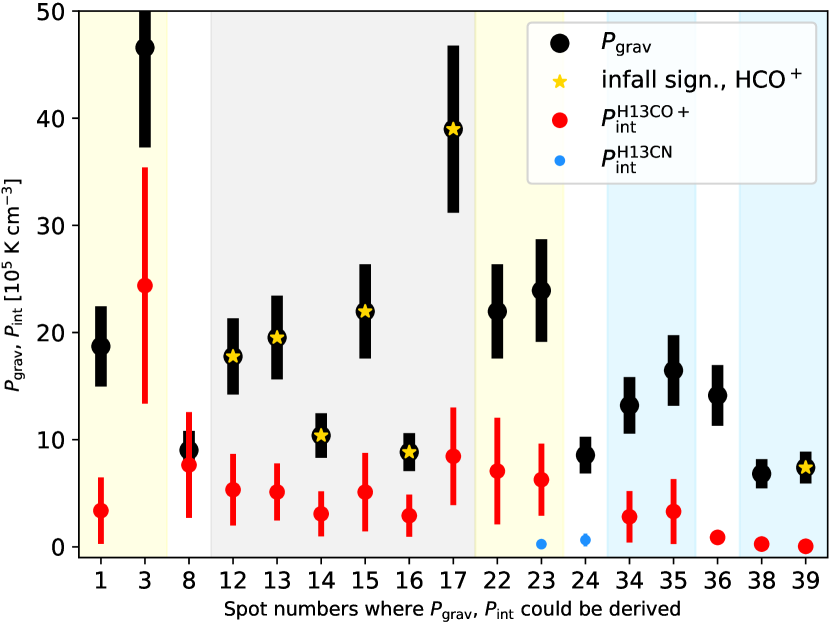
Figure 7: Left: Gravitational and turbulent energy densities (in 10^-10 erg cm^-3) with uncertainties. Right: Volume-averaged gravitational pressure and internal pressure (in 10⁵ K cm^-3), more precisely in the form of $P/k_{\rm B}$. They are indicated per spot number, where both pairs could be calculated; see the legends. The yellow stars mark the positions where the blue-red asymmetry of HCO⁺ lines revealed possible infall signatures. See Tables 1 and 2 for details, and Fig. 5 for the numbered analysis spots. Among the latters, light yellow background marks the spots which are along the central filament loop. Light grey background shows the spots in the southern filament, and light blue background indicates the ones along the north-western filament. See Sects. 3.4 and 4.2 for details.

4.2 Coherent structure with contracting cores

Gibb (2008) has noticed that NGC2071-N attracted very little study since the 1980s (Fukui et al., 1986; Iwata et al., 1988), which continues to hold ever since 2008. It is located at $\sim$20′ north of the NGC2071 reflection nebula, and its structures turned out to be more extended than the 0.7 pc-diameter clump first seen in C¹⁸O (Iwata et al., 1988). While NGC2071-N seems isolated from the rest of the L1630-North complex at the $\rm H_{2}$ column density level of $\sim 1\times 10^{22}$ cm^-2, it is well part of it within the contours at $\sim 2\times 10^{21}$ cm^-2. At this higher value, NGC2071-N looks more fragmented than, for example, the region of HH24–26, south of the NGC2068 reflection nebula (see Fig. 1 left at RA$\sim$05h46m, Dec$\sim$–00d15m). As we go down from this higher to the lower value, the column density contours become more extended around NGC2071-N, than around HH24–26. In other words, the same mass lies in a somewhat larger area in NGC2071-N. The high-column density fragments in our sub-region are the two centres, portions of surrounding filaments, and the extension at the north-west. (see e.g., Fig. 1 right). The basis of this simple comparison is the similar projected location of both sub-regions, i.e., north/south of a reflection nebula, respectively, on either side of the L1630-North complex (see Fig. 1 left). The above may mean that NGC2071-N still has a great potential to form more solar-type stars over a longer period of time.

At the time of Iwata et al. (1988), on the other hand, they inferred that this cloud is nearly in dynamical equilibrium, having calculated the same figures both for the gravitational energy and for total kinetic energy of internal turbulence. Then, Goldsmith et al. (1992) found their C¹⁸O clumps gravitationally unbound and deemed as probably transient structures.

We infer the current activity of this cloud from Fig. 7, the left panel of which shows that the gravitational energy densities dominate over the turbulent kinetic energy densities in most of the displayed positions. This same trend is also supported by the right panel of Fig. 7, that is that the volume-averaged gravitational pressures are higher than the internal turbulent pressures.

In spot #8, at the dense tip of the SE filament, the energy balance is less conclusive. Here, we measure one of the largest velocity dispersions based on the H¹³CO⁺ and HCN lines; $\sigma_{\rm NT}^{\rm H13CO+}$ is larger than that of the large-scale C¹⁸O, and $\sigma_{\rm NT}^{\rm HCN}$ is even larger than $\sigma_{\rm NT}^{\rm 13CO}$. However, the velocity dispersions of H¹³CO⁺ and HCN at #8 are fairly noisy that probably led to their overestimations, and therefore to higher turbulent energy densities and internal pressures.

Among the clumps along the central hub-ring, in particular #3 (around IRAS 05451+0037), #22, #23 that are located at junctions of filaments, we also observe higher estimated $u_{\rm turb}^{\rm H13CO+}$ and $P^{\rm H13CO+}_{\rm int}$ (Fig. 7). Besides the noisy lines, this might also arise from infalling material along the filamets, however more investigations on this are out of the scope of the present paper.

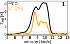
(a)

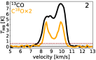
(b)

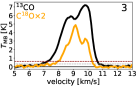
(c)

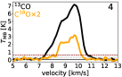
(d)

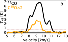
(e)

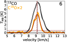
(f)

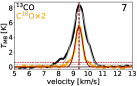
(g)

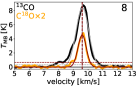
(h)

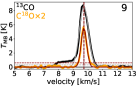
(i)

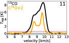
(j)

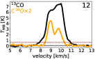
(k)

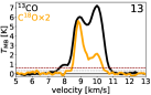
(l)

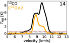
(m)

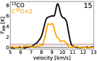
(n)

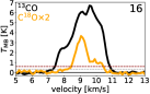
(o)

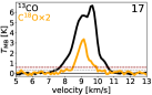
(p)

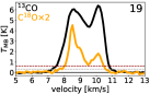
(q)

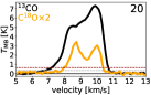
(r)

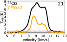
(s)

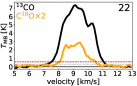
(t)

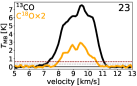
(u)

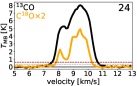
(v)

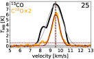
(w)

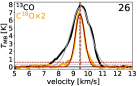
(x)

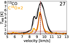
(y)

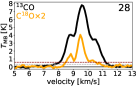
(z)

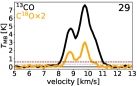
(aa)

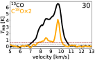
(ab)

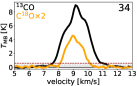
(ac)

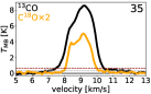
(ad)

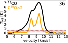
(ae)

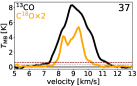
(af)

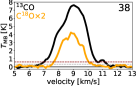
(ag)

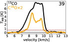
(ah)

Figure 9: ¹³CO(1–0) (black) and C¹⁸O(1–0) (orange) spectra averaged over the analysis spots where observed (see Fig. 5). When it is reasonable, a Gaussian fit and its peak position are also included. Dashed horizontal lines mark 6$\sigma$ rms thresholds; grey for the black spectra, red for the overplotted profiles. For details, see Sects. 3.3 and 3.4. Derived properties from these profiles are listed in Table 2.

In addition to the marked HCO⁺ infall candidates in Fig. 7, we can also identify blue-shifted asymmetric line profiles in the optically thick C¹⁸O (Fig. 9), in more than the already marked positions. Together with the indications that inside-out collapse has been detected in these clumps (Evans, 1999), the overall higher gravitational energy densities and pressures support the picture that gravity is acting stronger on spatial scales of $\sim$0.05 pc and is currently forming new stars in several spots of this region.

4.3 Hub with a double centre

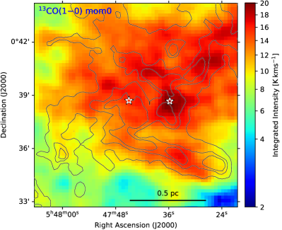
(a)

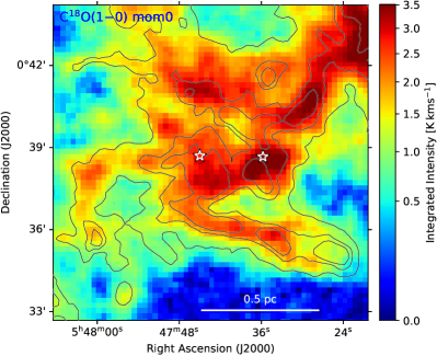
(b)

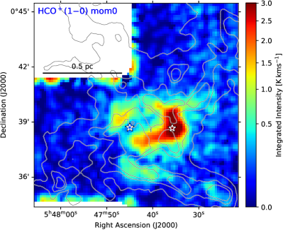
(c)

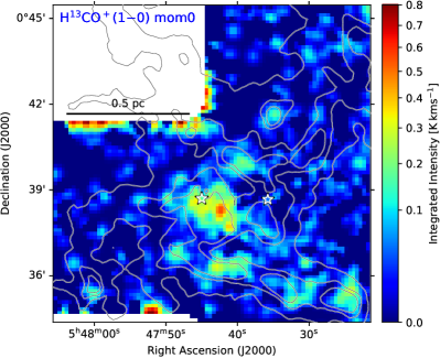
(d)

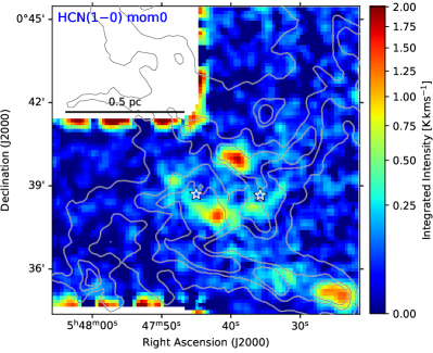
(e)

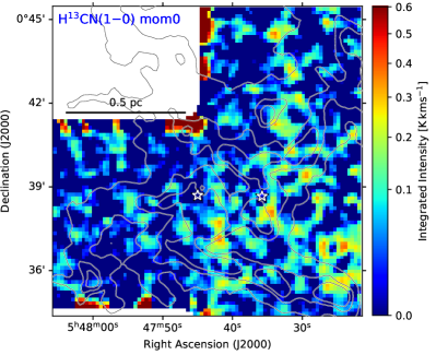
(f)

Figure 12: Integrated intensity (moment 0) maps of the hub centre (in main beam temperature) in the molecular lines indicated in the upper left corner. Higher intensity “strings of beads” at the map edges are artifacts. In all panels smoothed column density contours are overplotted, and the left and right white stars mark the locations of IRAS 05451+0037 and LkH$\alpha$ 316, resp.

The HGBS column density map shows a detailed filamentary structure, both at $A_{\rm V}\sim$ 5 and 10 mag contours (see Fig. 3 left), which was not known before. We suggest that a double centre may be formed in this hub, because the converging locations of the filaments S and SE, and NE and NW are somewhat offset along the hub-ring that is traced by a filament loop. In other words, the converging locations of filament pairs are offset. This offset is about 2.3′ ($0.27$ pc) measured from spot #3 to #22, (see Fig. 5), while there is almost the same projected distance between the IRAS and LkH$\alpha$ sources. Circle positions #3 and #22 correspond to the ammonia cores D and C, resp., defined by Iwata et al. (1988), while #3 contains IRAS 05451+0037 too. This span also matches the diameter of a ring-like structure that can be approximated from the combined emission at HCO⁺ and HCN (Fig. 12), given that the maxima of their integrated intensities are scattered along the hub-ring. This ring may indicate a transition and the connection between the hub and the filaments. We note that the junction of filament NE and that of filament NW with the hub-ring are not appearing as one projected point (as apparently the junction of filaments S and SE on the central ring), however the western section of the hub-ring, $\sim$0.1 pc around the nominal position of core C along the filaments, seems to be an active spot of star formation with dense cores and protostars (see Fig. 3 left).

Hub-filament systems are expected to feature one single centre on a larger scale, while they may break up after a closer look. Based on molecular line data, Treviño-Morales et al. (2019) extracted a complex filamentary network in Monoceros R2 ($d\sim$830 pc) also with a ring at the hub centre, where radially oriented filaments are joining from larger scales (see their Fig. 4.). Their hub-ring has a radius of approximately 0.30 pc, that we read from their figures, while that of ours is $\sim$0.13 pc that was estimated from a fitted circle to the closed loop of filament skeletons. There is a massive cluster forming in the Mon R2 filament hub (Rayner et al., 2017), unlike in NGC2071-N. Its most massive star IRS 1 ($\sim$12 $M_{\odot}$) appears close in projection to the location where multiple filaments arrive onto the Mon R2 hub-ring. IRS 1 is also associated with an ultra-compact HII region that may have helped clean the innermost ring area of the ¹³CO and C¹⁸O emission, while our hub centre is not devoid of the large-scale emission (see Fig. 12).

Their central hub (without the extending filament arms) has a radius of $\sim$1 pc within which the mass is about 1000 $M_{\odot}$, and the visual extinction is much higher than in NGC2071-N, above $\sim$20 mag, also derived from Herschel observations (Rayner et al., 2017). The latter authors suggest that star-formation is an on-going process in the Mon R2 hub that has already been regulated by feedback, which is again a substantial difference between our subregions. However, probably more such central hub-ring structures may exist on a larger scale of cloud properties.

4.4 At the centre of the hub

The sources in the central part of the hub, while it was not known that it is a hub, have been discussed in more detail by Aspin & Reipurth (2000) and Hillenbrand et al. (2012).

As it was mentioned before that this region is somewhat isolated, there are no such compact sources with nebulous emission in the vicinity either, which strengthens the confidence that IRAS 05451+0037 and LkH$\alpha$ 316 belong to the same neighbourhood (see also Sect. 3.1).

We have looked for these sources in archival data sets, and visualized the hub centre with a series of RGB images In Fig. 8 the left-hand side source is IRAS 05451+0037 and the lower right-hand side one is LkH$\alpha$ 316. The used surveys and their wavelengths are listed in Table 3.

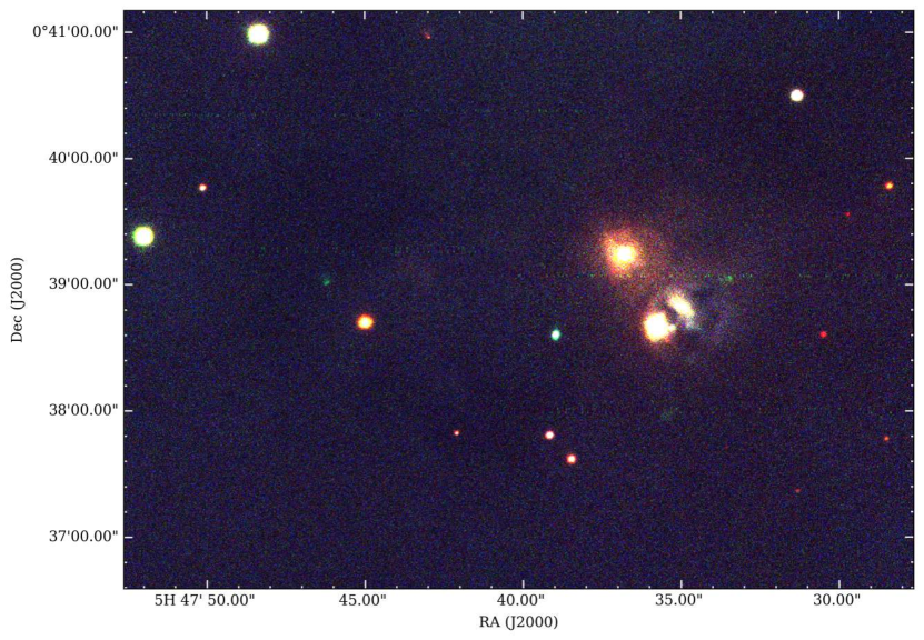
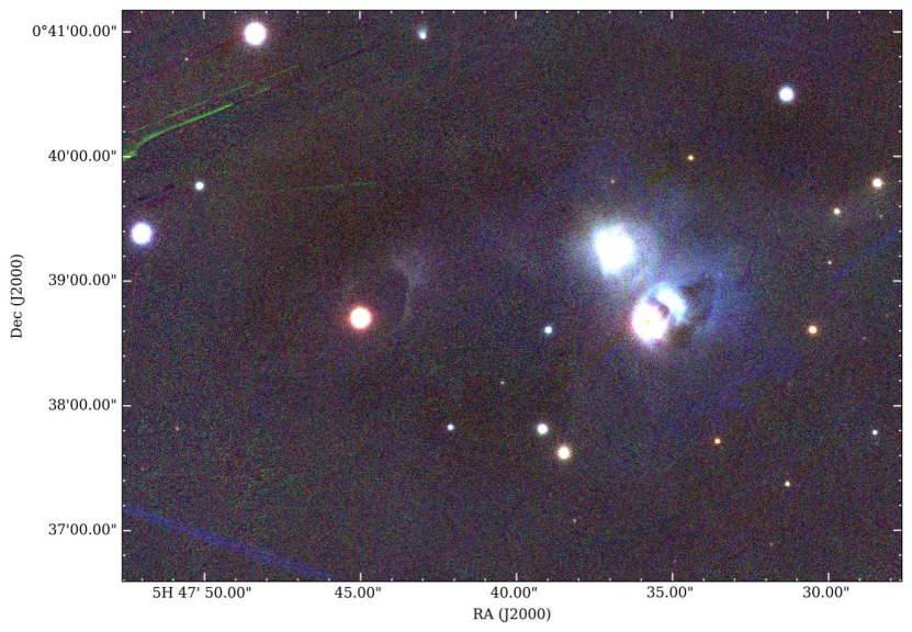
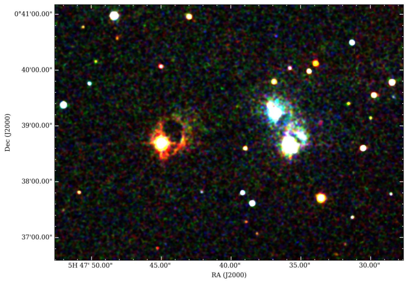
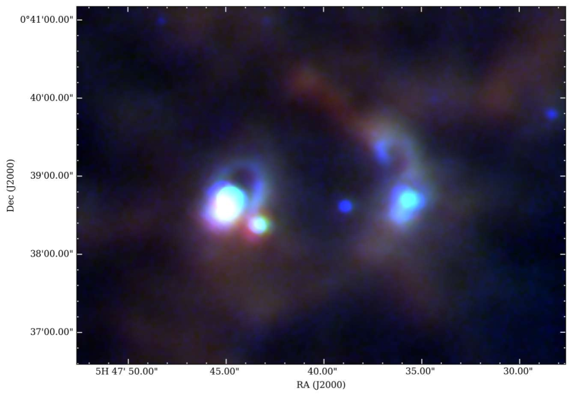
Figure 8: Zoomed RGB images on the double centre of the NGC2071-N filament hub. The left-hand side source, midplane, is IRAS 05451+0037 and the lower right-hand side one is LkH$\alpha$ 316. Top Left: SDSS i, r, g images (in the RGB order). Top Right: Pan-STARRS y, z, i filters. Bottom Left: 2MASS K_s, H, J filters. Bottom Right: Herschel 250, 160, and 100 $\mu$m images. All listed in the RGB order, while Table 3 lists the nominal wavelengths of all these filters and images from the shortest to the longest wavelengths.

Table 3: Summary of surveys and wavelengths providing images for Fig. 8. SDSS: Eisenstein et al. (2011); Pan-STARRS: Chambers et al. (2016); 2MASS: Skrutskie et al. (2006); Herschel: Pilbratt et al. (2010).

Figure panel	Fig. 8 top left			Fig. 8 top right			Fig. 8 bottom left			Fig. 8 bottom right
Survey	SDSS g	SDSS r	SDSS i	Pan-STR i	Pan-STR z	Pan-STR y	2MASS J	2MASS H	2MASS Ks	H 100	H 160	H 250
Wavelength [$\mu$m]	0.4686	0.6165	0.7481	0.7520	0.8660	0.9620	1.24	1.66	2.16	100	160	250

We note that throughout the paper we are using the position of IRAS 05451+0037 given by SIMBAD, which is referring to Gaia Collaboration (2018). This is almost identical to the one used by Hillenbrand et al. (2012) based on the associated SDSS source, but different from the position of this same IRAS source given by Wouterloot et al. (1988); Claussen et al. (1996); Aspin & Reipurth (2000). The location of the latter authors is $\sim$40″ west of ours, and the disagreement is most likely due to the large beam sizes of IRAS.

Aspin & Reipurth (2000) have identified new HH objects near compact reflection nebulae – that is our double centre in Fig. 8. Their HH 471 A-E jets and flows are associated with LkH$\alpha$ 316, and the earlier known HH 71 may as well, while HH 473-474 may be associated with the IRAS source as most likely exciting source. The new HH 472 seems to be associated with a faint and unknown source which positions are identified by SIMBAD as 2MASS J05473897+0038362. Aspin & Reipurth (2000) suggested that this unknown exciting source of HH 472 may be responsible for driving the outflow found by Fukui et al. (1986); Iwata et al. (1988) (see Sect. 4.5).

The right-hand side group of reflection nebulosities also appear in the $I$-band images of Aspin & Reipurth (2000). LkH$\alpha$ 316 is the lowest compact source, LkH$\alpha$ 316-neb lies $\sim$15″ north-west of it, and the 316/c component is the one $\sim$37″ north-east of them. LkH$\alpha$ 316-neb is only a nebulosity without a star. Most probably LkH$\alpha$ 316 and LkH$\alpha$ 316-neb are physically associated (Aspin & Reipurth, 2000), but we suggest that even 316/c may be part of this close system, visually based on the morphology of the diffuse gas and the curved material bridge that is best seen in the 2MASS and Herschel images (lower panels of Fig. 8).

Furthermore, another argument strengthening the physical association between all of the three LkH$\alpha$ 316 components is their locations in the column density map (see the contours in Fig. 4). The northern nebulosity is within the ammonia core C, at the junction of two filaments that can also be seen in the lower right panel of Fig. 8. Summarized in Sect. 3.2, at such locations matterial is deposited from which YSOs and infrared clusters may form more efficiently, which can be further channelled in between 316/c and the two other nebulosities. The integrated intensity map of HCO⁺(1–0) in Fig. 12, also suggests a connection between LkH$\alpha$ 316 and LkH$\alpha$ 316-neb, both being on the island of strongest emission. IRAS 05451+0037 is also found at the junction of filaments within ammonia core D, which was originally found to drive a bipolar CO outflow (Fukui et al., 1986; Iwata et al., 1988). Hillenbrand et al. (2012) derived a bolometric luminosity of $\sim 90\,L_{\odot}$ for IRAS 05451+0037, and presented for the first time its optical SDSS spectrum as well. From the analysis from SDSS up to JCMT/SCUBA wavelengths and models, they concluded that IRAS 05451+0037 is optically faint and far-infrared bright, and its SED is consistent with those of Class I and flat-spectrum YSOs. They suggest that there is still likely a significant circumstellar envelope that is feeding the extended massive disk.

They found that our IRAS source is the brightest in the region at mid-infrared wavelengths based on WISE images, although the nearby LkH$\alpha$ 316 and LkH$\alpha$ 316-neb become also quite strong by 25 $\mu$m.

Hillenbrand et al. (2012) saw nebulosity closely associated with the IRAS source as well at the 2MASS K and H bands that they did not find at shorter wavelengths. We suggest that this gas feature can be seen at shorter than 2MASS wavelengths too (top right panel of Fig. 8). At the wavelengths it is visible, it has a neat loop structure. The extent of this loop we measured from Pan-STARRS to Herschel images, and found to be 0.06–0.07 pc at the distance of 400 pc. This loop is rather thin and sharp, and the extent of it, from the compact source to the north-west corner, does not seem to vary with wavelength. These reflection nebulae around both hub centres indicate that there is interaction between the point sources and the cloud material.

4.5 CO outflow revisited

The large amorphous bipolar ¹²CO outflow in NGC2071-N was discovered by Fukui et al. (1986), and followed up by Iwata et al. (1988). They defined the outflow relatively old ($\tau\sim 1.7\times 10^{5}$ yr) and suggested that its driving source is IRAS 05451+0037, although it is off-axis to the east from the outflow lobes. In this same study they also presented a higher resolution, though not fully calibrated CO map, where there is indication that the lobes are extended towards the IRAS source. They then suggested that the outflow has a U-shape with the IRAS source at the bottom of it. The red-shifted CO lobe peaks nearly in between IRAS 05451+0037 and LkH$\alpha$ 316, which also complicates the interpretation with the IRAS source as the origin. Goldsmith et al. (1992) still found the origin of this outflow less clearly identifiable.

Then Aspin & Reipurth (2000) suggested their HH 472 jet and its unknown source to be the driving source of the outflow, as they are located between the blue and red lobes. This molecular outflow and the HH objects are also misaligned, perhaps indicating a stronger or differently directed flow in the past (Hillenbrand et al., 2012).

Interestingly, the complete loop-shaped nebulosity around IRAS 05451+0037 (Fig. 8) extends from the point source towards north-west, in which direction there is the apparent centre of the outflow, however from our fine-detailed ¹³CO(1–0) molecular line data, plotting channel maps, we cannot confirm this outflow, and it is more probable that its SE-NW axis, interpreted at much lower resolution, corresponds to the dense features we can also see in column density along the SE-NW axis (e.g., Fig. 3 left).

5 Conclusions

We have presented Herschel, molecular line, and archival data sets, including 100 $\mu$m Herschel images, IRAM 30 m, and NRO 45 m observatons over a newly resolved hub-filament structure in NGC2071-North featuring a double centre. Our main results and conclusions are summarized as follows:

1. We confirm that NGC2071-North is part of the L1630 North complex at $d\sim 400$ pc, and is not affected by the Barnard’s Loop (nearby in projection) which may be at a closer distance ($\sim$180 pc).

2. The Herschel H₂ column density image reveals a $\sim 1.5\times 1.5$ pc-size filamentary hub structure with curved arms, containing $\sim$500 $M_{\odot}$ above $A_{V}\sim 5$ mag. The 100 $\mu$m emission concentrates in the central part of the filament hub, at IRAS 05451+0037 and the emission star LkH$\alpha$ 316, and features diffuse lobes and loops around them.

3. We have estimated the energy balance by calculating gravitational and turbulent kinetic energy densities, as well as gravitational and internal pressures within 42 spots, with 25″ radius, along the filaments. From these comparisons, together with finding several infall candidates in HCO⁺ and C¹⁸O, we conclude that gravity dominates on small scales, and NGC2071-N is currently forming stars.

4. Planck POS magnetic field lines reveal a loop structure east of NGC2071, extending up to NGC2071-N. This results in east-west B-field lines in the east of the hub, and north-south running field lines in the west of the filament hub. This closely perpendicular B-field structure may be an efficient configuration for gathering material at this relatively isolated location.

5. We suggest that a double centre could be formed in this hub, because the converging locations of two filament pairs are offset. This offset is 2.3′($0.27$ pc) that also matches the diameter of a central hub-ring that is seen in column density, traced by filaments, and in HCO⁺ and HCN, which may indicate a transition and connection between the hub and the filaments.

6. We argue that not only two, but all of the three components of the LkH$\alpha$ 316 young star (along with 316-neb and 316/c) are in physical association due to the location of the latter at the junction of two filaments. We find that the clear gas loop feature around IRAS 05451+0037 can already be seen at shorter than 2MASS wavelengths. The extent of this loop we measured to be 0.06–0.07 pc which does not seem to vary with wavelength.

7. We have revisited the CO outflow, discovered by Fukui et al. (1986), and we do not seem to find its lobes in our high-resolution ¹³CO data.

Data Availability

The PACS and SPIRE maps, the $Herschel$ column density and temperature maps, as well as the dense core lists extracted from them in the whole Orion B region are publicly available at the $Herschel$ Gould Belt Survey Archive: http://gouldbelt-herschel.cea.fr/archives. Additional molecular line maps presented in this paper are available at http://dx.doi.org/xxxx.yyyyy.

Appendix A Averaged Spectra

Appendix B Integrated Intensity Maps

References

- Alina et al. (2019) Alina D., Ristorcelli I., Montier L., Abdikamalov E., Juvela M., Ferrière K., Bernard J. P., Micelotta E. R., 2019, MNRAS, 485, 2825
- André et al. (2010) André P., et al., 2010, A&A, 518, L102+
- André et al. (2014) André P., Di Francesco J., Ward-Thompson D., Inutsuka S.-I., Pudritz R. E., Pineda J. E., 2014, in Protostars and Planets VI, ed. H. Beuther et al.. p. 27 (arXiv:1312.6232), doi:10.2458/azu_uapress_9780816531240-ch002
- André et al. (2022) André P., Palmeirim P., Arzoumanian D., 2022, A&A, 667, L1
- Anthony-Twarog (1982) Anthony-Twarog B. J., 1982, AJ, 87, 1213
- Arzoumanian et al. (2011) Arzoumanian D., et al., 2011, A&A, 529, L6
- Arzoumanian et al. (2019) Arzoumanian D., et al., 2019, A&A, 621, A42
- Aspin & Reipurth (2000) Aspin C., Reipurth B., 2000, MNRAS, 311, 522
- Bally (2008) Bally J., 2008, Overview of the Orion Complex. p. 459
- Benedettini et al. (2018) Benedettini M., et al., 2018, A&A, 619, A52
- Bertoldi & McKee (1992) Bertoldi F., McKee C. F., 1992, ApJ, 395, 140
- Bohlin et al. (1978) Bohlin R. C., Savage B. D., Drake J. F., 1978, ApJ, 224, 132
- Bonnor (1956) Bonnor W. B., 1956, MNRAS, 116, 351
- Carter et al. (2012) Carter M., et al., 2012, A&A, 538, A89
- Chambers et al. (2016) Chambers K. C., et al., 2016, arXiv e-prints, p. arXiv:1612.05560
- Chen et al. (2016) Chen C.-Y., King P. K., Li Z.-Y., 2016, ApJ, 829, 84
- Claussen et al. (1996) Claussen M. J., Wilking B. A., Benson P. J., Wootten A., Myers P. C., Terebey S., 1996, ApJS, 106, 111
- Cutri et al. (2003) Cutri R. M., et al., 2003, VizieR Online Data Catalog, p. II/246
- Dale & Bonnell (2011) Dale J. E., Bonnell I., 2011, MNRAS, 414, 321
- Dewangan et al. (2015) Dewangan L. K., Luna A., Ojha D. K., Anandarao B. G., Mallick K. K., Mayya Y. D., 2015, ApJ, 811, 79
- Dhabal et al. (2018) Dhabal A., Mundy L. G., Rizzo M. J., Storm S., Teuben P., 2018, ApJ, 853, 169
- Dunham et al. (2011) Dunham M. K., Rosolowsky E., Evans Neal J. I., Cyganowski C., Urquhart J. S., 2011, ApJ, 741, 110
- Eisenstein et al. (2011) Eisenstein D. J., et al., 2011, AJ, 142, 72
- Evans (1999) Evans Neal J. I., 1999, ARA&A, 37, 311
- Fiorellino et al. (2021) Fiorellino E., et al., 2021, MNRAS, 500, 4257
- Fukui et al. (1986) Fukui Y., Sugitani K., Takaba H., Iwata T., Mizuno A., Ogawa H., Kawabata K., 1986, ApJ, 311, L85
- Gaia Collaboration (2018) Gaia Collaboration 2018, VizieR Online Data Catalog, p. I/345
- Gibb (2008) Gibb A. G., 2008, Star Formation in NGC 2068, NGC 2071, and Northern L1630. p. 693
- Goldsmith et al. (1992) Goldsmith P. F., Margulis M., Snell R. L., Fukui Y., 1992, ApJ, 385, 522
- Greenfield et al. (2013) Greenfield P., et al., 2013, Astropy: Community Python library for astronomy (ascl:1304.002)
- Hacar et al. (2022) Hacar A., Clark S., Heitsch F., Kainulainen J., Panopoulou G., Seifried D., Smith R., 2022, arXiv e-prints, p. arXiv:2203.09562
- Hatchell et al. (2005) Hatchell J., Richer J. S., Fuller G. A., Qualtrough C. J., Ladd E. F., Chandler C. J., 2005, A&A, 440, 151
- He et al. (2015) He Y.-X., et al., 2015, MNRAS, 450, 1926
- Hillenbrand et al. (2012) Hillenbrand L. A., Knapp G. R., Padgett D. L., Rebull L. M., McGehee P. M., 2012, AJ, 143, 37
- Iwata et al. (1988) Iwata T., Fukui Y., Ogawa H., 1988, ApJ, 325, 372
- Johnstone et al. (2004) Johnstone D., Di Francesco J., Kirk H., 2004, ApJ, 611, L45
- Kirk, H. et al. (2006) Kirk, H. Johnstone D., Di Francesco J., 2006, ApJ, 646, 1009
- Kirk et al. (2016a) Kirk H., et al., 2016a, ApJ, 817, 167
- Kirk et al. (2016b) Kirk H., et al., 2016b, ApJ, 817, 167
- Koch & Rosolowsky (2015) Koch E. W., Rosolowsky E. W., 2015, MNRAS, 452, 3435
- Könyves et al. (2015) Könyves V., et al., 2015, A&A, 584, A91
- Könyves et al. (2020) Könyves V., et al., 2020, A&A, 635, A34
- Ladjelate et al. (2020) Ladjelate B., et al., 2020, A&A, 638, A74
- Lallement et al. (2014) Lallement R., Vergely J.-L., Valette B., Puspitarini L., Eyer L., Casagrande L., 2014, A&A, 561, A91
- Li et al. (2013) Li H.-b., Fang M., Henning T., Kainulainen J., 2013, MNRAS, 436, 3707
- Lyo et al. (2021) Lyo A. R., et al., 2021, ApJ, 918, 85
- Marsh et al. (2016) Marsh K. A., et al., 2016, MNRAS, 459, 342
- Megeath et al. (2012) Megeath S. T., et al., 2012, AJ, 144, 192
- Menten et al. (2007) Menten K. M., Reid M. J., Forbrich J., Brunthaler A., 2007, A&A, 474, 515
- Miville-Deschênes et al. (2017) Miville-Deschênes M.-A., Murray N., Lee E. J., 2017, ApJ, 834, 57
- Myers (2009) Myers P. C., 2009, ApJ, 700, 1609
- Myers et al. (1996) Myers P. C., Mardones D., Tafalla M., Williams J. P., Wilner D. J., 1996, ApJ, 465, L133
- Nakamura & Li (2008) Nakamura F., Li Z.-Y., 2008, ApJ, 687, 354
- Ochsendorf et al. (2015) Ochsendorf B. B., Brown A. G. A., Bally J., Tielens A. G. G. M., 2015, ApJ, 808, 111
- Onishi et al. (1998) Onishi T., Mizuno A., Kawamura A., Ogawa H., Fukui Y., 1998, ApJ, 502, 296
- Palmeirim et al. (2013) Palmeirim P., et al., 2013, A&A, 550, A38
- Panopoulou et al. (2022) Panopoulou G. V., Clark S. E., Hacar A., Heitsch F., Kainulainen J., Ntormousi E., Seifried D., Smith R. J., 2022, A&A, 657, L13
- Pattle et al. (2015) Pattle K., et al., 2015, MNRAS, 450, 1094
- Peretto et al. (2006) Peretto N., André P., Belloche A., 2006, A&A, 445, 979
- Peretto et al. (2012) Peretto N., et al., 2012, A&A, 541, A63
- Peretto et al. (2013) Peretto N., et al., 2013, A&A, 555, A112
- Pilbratt et al. (2010) Pilbratt G. L., et al., 2010, A&A, 518, L1+
- Pineda et al. (2022) Pineda J. E., et al., 2022, arXiv e-prints, p. arXiv:2205.03935
- Planck Collaboration et al. (2016) Planck Collaboration et al., 2016, A&A, 586, A138
- Rayner et al. (2017) Rayner T. S. M., et al., 2017, A&A, 607, A22
- Rygl et al. (2013) Rygl K. L. J., Wyrowski F., Schuller F., Menten K. M., 2013, A&A, 549, A5
- Sadavoy et al. (2015) Sadavoy S. I., Shirley Y., Di Francesco J., Henning T., Currie M. J., André P., Pezzuto S., 2015, ApJ, 806, 38
- Sault et al. (1995) Sault R. J., Teuben P. J., Wright M. C. H., 1995, in Shaw R. A., Payne H. E., Hayes J. J. E., eds, Astronomical Society of the Pacific Conference Series Vol. 77, Astronomical Data Analysis Software and Systems IV. p. 433 (arXiv:astro-ph/0612759)
- Schlafly et al. (2014) Schlafly E. F., et al., 2014, ApJ, 786, 29
- Schneider et al. (2010) Schneider N., et al., 2010, A&A, 518, L83
- Schneider et al. (2012) Schneider N., et al., 2012, A&A, 540, L11
- Shimajiri et al. (2017) Shimajiri Y., et al., 2017, A&A, 604, A74
- Skrutskie et al. (2006) Skrutskie M. F., et al., 2006, AJ, 131, 1163
- Snell (1989) Snell R. L., 1989, Molecular Outflows. p. 231, doi:10.1007/BFb0114872
- Soler (2019) Soler J. D., 2019, A&A, 629, A96
- Soler & Hennebelle (2017) Soler J. D., Hennebelle P., 2017, A&A, 607, A2
- Soler et al. (2013) Soler J. D., Hennebelle P., Martin P. G., Miville-Deschênes M. A., Netterfield C. B., Fissel L. M., 2013, ApJ, 774, 128
- Sousbie (2011) Sousbie T., 2011, MNRAS, 414, 350
- Tahani et al. (2018) Tahani M., Plume R., Brown J. C., Kainulainen J., 2018, A&A, 614, A100
- Tenorio-Tagle (1982) Tenorio-Tagle G., 1982, in Roger R. S., Dewdney P. E., eds, Astrophysics and Space Science Library Vol. 93, Regions of Recent Star Formation. pp 1–13, doi:10.1007/978-94-009-7778-5_1
- Traficante et al. (2017) Traficante A., Fuller G. A., Billot N., Duarte-Cabral A., Merello M., Molinari S., Peretto N., Schisano E., 2017, MNRAS, 470, 3882
- Treviño-Morales et al. (2019) Treviño-Morales S. P., et al., 2019, A&A, 629, A81
- Wouterloot et al. (1988) Wouterloot J. G. A., Walmsley C. M., Henkel C., 1988, A&A, 203, 367
- Zucker et al. (2019) Zucker C., Speagle J. S., Schlafly E. F., Green G. M., Finkbeiner D. P., Goodman A. A., Alves J., 2019, ApJ, 879, 125