A Sequential Quadratic Programming Method with High Probability Complexity Bounds for Nonlinear Equality Constrained Stochastic Optimization

Abstract

A step-search sequential quadratic programming method is proposed for solving nonlinear equality constrained stochastic optimization problems. It is assumed that constraint function values and derivatives are available, but only stochastic approximations of the objective function and its associated derivatives can be computed via inexact probabilistic zeroth- and first-order oracles. Under reasonable assumptions, a high-probability bound on the iteration complexity of the algorithm to approximate first-order stationarity is derived. Numerical results on standard nonlinear optimization test problems illustrate the advantages and limitations of our proposed method.

1 Introduction

In this paper, we propose a step-search sequential quadratic programming (SQP) algorithm for solving nonlinear equality-constrained stochastic optimization problems of the form

$$\min_{x\in\mathbb{R}^{n}}\ f(x)\quad\text{s.t.}\ c(x)=0,$$ (1.1)

where $f:\mathbb{R}^{n}\to\mathbb{R}$ and $c:\mathbb{R}^{n}\to\mathbb{R}^{m}$ are both continuously differentiable. We consider the setting in which exact function and derivative information of the objective function is unavailable, instead, only random estimates of the objective function $\bar{f}(x;\Xi^{0}(x))\approx f(x)$ and its first-order derivative $\bar{g}(x;\Xi^{1}(x))\approx\nabla f(x)$ are available via inexact probabilistic oracles, where $\Xi^{0}(x)$ (with probability space $(\Omega^{0},\mathcal{F}_{\Omega^{0}},P^{0})$) and $\Xi^{1}(x)$ (with probability space $(\Omega^{1},\mathcal{F}_{\Omega^{1}},P^{1})$) denote the underlying randomness in the objective function and gradient estimates, respectively. On the other hand, the constraint function value $c(x)$ and its Jacobian $\nabla c(x)^{T}$ are assumed to be available. Such deterministically constrained stochastic optimization problems arise in multiple science and engineering applications, including but not limited to computer vision [37], multi-stage optimization [39], natural language processing [30], network optimization [9], and PDE-constrained optimization [35].

The majority of the methods proposed in the literature for solving deterministically equality-constrained stochastic optimization problems follow either projection or penalty approaches. The former type of methods (e.g., stochastic projection methods [21, 23, 24, 25]) require that the feasible region satisfies strict conditions, to ensure well-definedness, that are not satisfied by general nonlinear functions and thus are not readily applicable. In contrast, the latter, stochastic penalty methods [14, 34], do not impose such conditions on the feasible region. These methods transform constrained problems into unconstrained problems via a constraint penalization term in the objective function and apply stochastic algorithms to solve the transformed unconstrained optimization problems. Stochastic penalty methods are easy to implement and well-studied, however, the empirical performance of such methods is sensitive to parameter choices and ill-conditioning, and is usually inferior to paradigms that treat constraints as constraints.

Recently, a class of stochastic SQP methods has been developed for solving (1.1). These methods outperform stochastic penalty methods empirically and have convergence guarantees in expectation [7, 28]. In [7], the authors propose an objective-function-free stochastic SQP method with adaptive step sizes for the fully stochastic regime. In contrast, in [28], the authors propose a stochastic step search (referred to as line search in the paper [28]) SQP method for the setting in which the errors in the function and derivative approximations can be diminished. We note that several algorithm choices in the two papers [7, 28], e.g., merit functions and merit parameters, are different. Several other extensions have been proposed [6, 17, 3, 8, 27, 32], and very few of these works (or others in the literature) derive worst-case iteration complexity (or sample complexity) due to the difficulties that arise because of the constrained setting and the stochasticity. Notable exceptions are, [16] where the authors provide convergence rates (and complexity guarantees) for the algorithm proposed in [7], and [3, 29] that provide complexity bounds for variants of the stochastic SQP methods under additional assumptions and in the setting in which the errors can be diminished. We note that, with the exception of [32], all methods mentioned above assume access to unbiased estimates of the gradients (and function values where necessary), whereas in this paper, we propose an algorithm that can handle biased function and gradient estimates.

For all aforementioned methods, the most vital ingredient is the quality and reliability of the random estimates of the objective function and its derivatives. In our setting, neither the objective function nor its derivatives are assumed to be directly accessible, only stochastic approximations of them are accessible to the algorithm in the form of inexact probabilistic zeroth-order and first-order oracles (precise definitions will be introduced in Section 2.3). Such oracles have been proposed and utilized in several works; e.g., [22, 12, 20, 1]. Moreover, these probabilistic oracles and their variants have been proposed for direct-search methods [20, 36], trust-region methods [1, 10, 15, 19], and step-search methods [13, 33, 28, 2]. We note that only [28] considers the setting with (equality) constraints, but iteration complexity (or sample complexity) results are not provided.

1.1 Contributions

In this paper, we design, analyze, and implement a step-search SQP (SS-SQP) method for solving nonlinear equality-constrained stochastic optimization problems where exact constraint function values and derivatives are available, but only stochastic approximations of the objective function and its associated derivatives can be computed. These stochastic approximations are computed via inexact probabilistic zeroth- and first-order oracles, which are similar to those in [22], with parameters controlling the accuracy and reliability of the approximations, and allowing for biased approximations. Our proposed algorithm is inspired by state-of-the-art line search SQP methods [11] in conjunction with the recent stochastic adaptive step-search framework developed in [22] for the unconstrained stochastic setting. At every iteration, the algorithm constructs a model of the reduction in the merit function that serves the dual purpose of a measure of sufficient progress (part of the step size computation) and a proxy for convergence. To mitigate the challenges that arise due to the noise in the objective function evaluations, our step-search method employs a relaxed sufficient decrease condition similar to that proposed in [4]. Under reasonable assumptions, we provide a high probability worst-case iteration complexity bound for the proposed algorithm. Specifically, we prove that with overwhelmingly high probability, our proposed algorithm generates a first-order $\varepsilon$-stationary iterate in $\mathcal{O}(\varepsilon^{-2})$ iterations, where $\varepsilon$ is bounded away from zero and its lower bound is dictated by the noise and bias in the zeroth- and first-order oracles. The complexity bound derived matches that of the deterministic algorithm provided in [16]. There are two key differences between our paper and [16]: $(i)$ our algorithm requires access to the objective function whereas the method in [16] is objective-function-free; and $(ii)$ our first-order oracle provides estimates with sufficient accuracy only with some probability and can provide arbitrarily bad estimates otherwise. Finally, numerical results on standard nonlinear equality-constrained test problems [18] illustrate the efficiency and efficacy of our proposed algorithm.

1.2 Notation

Let $\mathbb{R}$ denote the set of real numbers, $\mathbb{R}^{n}$ denote the set of $n$-dimensional real vectors, $\mathbb{R}^{m\times n}$ denote the set of $m$-by-$n$-dimensional real matrices, $\mathbb{N}$ denote the set of natural numbers, and $\mathbb{S}^{n}$ denote the set of $n$-by-$n$-dimensional real symmetric matrices. For any $a\in\mathbb{R}$, let $\mathbb{R}_{>a}$ ($\mathbb{R}_{\geq a}$) denote the set of real numbers strictly larger than (larger than or equal to) $a$. We use $\|\cdot\|$ to denote the $\ell_{2}$-norm. We use $k\in\mathbb{N}$ as the iteration counter of the algorithm, and for brevity, we use a subscript $k$ for denoting information at the $k$th iterate, e.g., $f_{k}:=f(x_{k})$. All quantities with over-bars are stochastic, e.g., $\bar{f}(x;\Xi^{0}(x))$ and $\bar{g}(x;\Xi^{1}(x))$ (see Section 2.3), and $\bar{f}(x;\xi^{0}(x))$ (resp. $\bar{g}(x;\xi^{1}(x))$) denote realizations of $\bar{f}(x;\Xi^{0}(x))$ (resp. $\bar{g}(x;\Xi^{1}(x))$).

1.3 Organization

The rest of this paper is organized as follows. The algorithmic framework is introduced in Section 2. The analysis of the algorithm is established in Section 3. We report numerical results in Section 4. Concluding remarks and future research directions are given in Section 5.

2 Algorithm

To solve (1.1), we design an iterative algorithm based on the SQP paradigm that generates: $(i)$ a primal iterate sequence $\{x_{k}\}$, $(ii)$ a primal trial iterate sequence $\{x_{k}^{+}\}$, $(iii)$ a primal search direction sequence $\{\bar{d}_{k}\}$, $(iv)$ a dual iterate sequence $\{\bar{y}_{k}\}$, $(v)$ a step size sequence $\{\alpha_{k}\}$, $(vi)$ a merit parameter sequence $\{\bar{\tau}_{k}\}$, and, $(vii)$ a trial merit parameter sequence $\{\bar{\tau}^{\rm trial}_{k}\}$. We discuss each of these sequences in below. We make the following assumption throughout the remainder of this paper.

Assumption 2.1.

Let ${\cal X}\subseteq\mathbb{R}^{n}$ be an open convex set including iterates $\{x_{k}\}$ and trial iterates $\{x_{k}^{+}\}$. The objective function $f:\mathbb{R}^{n}\to\mathbb{R}$ is continuously differentiable and bounded below over ${\cal X}$. The objective gradient function $\nabla f:\mathbb{R}^{n}\to\mathbb{R}^{n}$ is $L$-Lipschitz continuous and bounded over ${\cal X}$. The constraint function $c:\mathbb{R}^{n}\to\mathbb{R}^{m}$ (where $m\leq n$) is continuously differentiable and bounded over ${\cal X}$, and each gradient $\nabla c_{i}:\mathbb{R}^{n}\to\mathbb{R}^{n}$ is $\gamma_{i}$-Lipschitz continuous and bounded over ${\cal X}$ for all $i\in\{1,\ldots,m\}$. The singular values of $J:=\nabla c^{T}$ are bounded away from zero over ${\cal X}$.

Assumption 2.1 is a standard assumption in the deterministic constrained optimization literature [31]. Under Assumption 2.1, there exist constants $\{\kappa_{g},\kappa_{c},\kappa_{J},\kappa_{\sigma}\}\subset\mathbb{R}_{>0}$ and $f_{\inf}\in\mathbb{R}$ such that for all $k\in\mathbb{N}$,

$$f_{\inf}\leq f_{k},\ \|\nabla f_{k}\|\leq\kappa_{g},\ \|c_{k}\|_{1}\leq\kappa_{c},\ \|J_{k}\|\leq\kappa_{J},\text{ and }\|(J_{k}J_{k}^{T})^{-1}\|\leq\kappa_{\sigma}.$$

We should note that by Assumption 2.1, linear independence constraint qualifications (LICQ) hold. Moreover, under Assumption 2.1, for all $x\in\mathbb{R}^{n}$, $d\in\mathbb{R}^{n}$ and $\alpha\in\mathbb{R}_{\geq 0}$ it follows that

$$f(x+\alpha d) \leq f(x)+\alpha\nabla f(x)^{T}d+\tfrac{L}{2}\alpha^{2}\|d\|^{2}$$ (2.1)

$$\text{and}\ \ \|c(x+\alpha d)\|_{1} \leq\|c(x)+\alpha\nabla c(x)^{T}d\|_{1}+\tfrac{\Gamma}{2}\alpha^{2}\|d\|^{2},\ \ \text{where $\Gamma=\sum_{i=1}^{m}\gamma_{i}$.}$$

In this paper, we are particularly interested in finding some primal-dual iterate $(x,y)\in\mathbb{R}^{n}\times\mathbb{R}^{m}$ that satisfies the first-order stationarity conditions of (1.1). To this end, let $\mathcal{L}:\mathbb{R}^{n}\times\mathbb{R}^{m}\rightarrow\mathbb{R}$ be the Lagrangian of (1.1), defined as

$$\mathcal{L}(x,y)=f(x)+y^{T}c(x),$$ (2.2)

where $y\in\mathbb{R}^{m}$ are the dual variables. The first-order stationarity conditions for (1.1), which are necessary by Assumption 2.1 (due to the inclusion of the LICQ), are

$$0=\begin{bmatrix}\nabla_{x}\mathcal{L}(x,y)\\ \nabla_{y}\mathcal{L}(x,y)\end{bmatrix}=\begin{bmatrix}\nabla f(x)+\nabla c(x)y\\ c(x)\end{bmatrix}.$$ (2.3)

In the remainder of this section we introduce the key algorithmic components: the merit function and its associated models, the search direction computation and merit parameter updating mechanism, and the inexact probabilistic zeroth- and first-order oracles. The main algorithm is Algorithm 1.

2.1 Merit function

The merit function $\phi:\mathbb{R}^{n}\times\mathbb{R}_{>0}\to\mathbb{R}$ is defined as

$$\phi(x,\tau):=\tau f(x)+\|c(x)\|_{1},$$ (2.4)

where $\tau\in\mathbb{R}_{>0}$, the merit parameter, acts as a balancing parameter between the objective function and the constraint violation. Given the gradient (approximation) $g\in\mathbb{R}^{n}$ and a search direction $d\in\mathbb{R}^{n}$, the model of merit function $l:\mathbb{R}^{n}\times\mathbb{R}_{>0}\times\mathbb{R}^{n}\times\mathbb{R}^{n}\to\mathbb{R}$ is defined as

$$l(x,\tau,g,d):=\tau(f(x)+g^{T}d)+\|c(x)+\nabla c(x)^{T}d\|_{1}.$$

Given a search direction $d\in\mathbb{R}^{n}$ that satisfies linearized feasibility, i.e., $c(x)+\nabla c(x)^{T}d=0$, the reduction in the model of the merit function $\Delta l:\mathbb{R}^{n}\times\mathbb{R}_{>0}\times\mathbb{R}^{n}\times\mathbb{R}^{n}\to\mathbb{R}$ is defined as

$$\Delta l(x,\tau,g,d):= l(x,\tau,g,0)-l(x,\tau,g,d)$$ (2.5)

$$= -\tau g^{T}d+\|c(x)\|_{1}-\|c(x)+\nabla c(x)^{T}d\|_{1}$$

$$= -\tau g^{T}d+\|c(x)\|_{1}.$$

We use the reduction in the model of the merit function (2.5) to monitor the progress made by our proposed algorithm. We discuss this in more detail in Section 2.2.

2.2 Algorithmic components

We now establish how to: $(i)$ compute the primal search direction sequence $\{\bar{d}_{k}\}$, $(ii)$ update the merit parameter sequence $\{\bar{\tau}_{k}\}$, and $(iii)$ update the primal iterate sequence $\{x_{k}\}$. These sequences depend on the approximation of the gradient of the objective function sequence $\{\bar{g}(x_{k};\Xi^{1}(x_{k}))\}$. Let $\bar{g}(x_{k};\xi^{1}(x_{k}))$ denote the realization of $\bar{g}(x_{k};\Xi^{1}(x_{k}))$. To simplify the notation, in this subsection we drop the dependence on the randomness, e.g., $\bar{g}_{k}=\bar{g}(x_{k};\xi^{1}(x_{k}))$.

At each iteration $k\in\mathbb{N}$, the primal search direction $\bar{d}_{k}\in\mathbb{R}^{n}$ and the dual variable $\bar{y}_{k}\in\mathbb{R}^{m}$ are computed by solving the linear system of equations

$$\begin{bmatrix}H_{k}&J_{k}^{T}\\ J_{k}&0\end{bmatrix}\begin{bmatrix}\bar{d}_{k}\\ \bar{y}_{k}\end{bmatrix}=-\begin{bmatrix}\bar{g}_{k}\\ c_{k}\end{bmatrix},$$ (2.6)

where $\{H_{k}\}$ satisfies the following assumption.

Assumption 2.2.

For all $k\in\mathbb{N}$, $H_{k}\in\mathbb{S}^{n}$ is chosen independently from $\bar{g}_{k}$. Moreover, there exist constants $\{\kappa_{H},\zeta\}\subset\mathbb{R}_{>0}$ such that for all $k\in\mathbb{N}$, $\|H_{k}\|\leq\kappa_{H}$ and $u^{T}H_{k}u\geq\zeta\|u\|^{2}$ for any $u\in\operatorname{Null}(J_{k})$.

It is well known that under Assumptions 2.1 and 2.2, there is a unique solution $(\bar{d}_{k},\bar{y}_{k})$ to (2.6), and, thus, the vectors $\bar{d}_{k}\in\mathbb{R}^{n}$ and $\bar{y}_{k}\in\mathbb{R}^{m}$ are well-defined [31].

Next, we present the merit parameter updating mechanism. Given constants $\{\epsilon_{\tau},\sigma\}\subset(0,1)$, for all $k\in\mathbb{N}$, we compute $\bar{\tau}_{k}$ via

$$\bar{\tau}_{k}\leftarrow\begin{cases}\bar{\tau}_{k-1}\ &\text{if }\bar{\tau}_{k-1}\leq\bar{\tau}^{\rm trial}_{k};\\ \min\left\{(1-\epsilon_{\tau})\bar{\tau}_{k-1},\bar{\tau}^{\rm trial}_{k}\right\}&\text{otherwise,}\end{cases}$$ (2.7)

where

$$\bar{\tau}^{\rm trial}_{k}\leftarrow\begin{cases}\infty\ &\text{if }\bar{g}_{k}^{T}\bar{d}_{k}+\max\left\{\bar{d}_{k}^{T}H_{k}\bar{d}_{k},0\right\}\leq 0;\\ \tfrac{(1-\sigma)\|c_{k}\|_{1}}{\bar{g}_{k}^{T}\bar{d}_{k}+\max\left\{\bar{d}_{k}^{T}H_{k}\bar{d}_{k},0\right\}}&\text{otherwise.}\end{cases}$$ (2.8)

The merit parameter updating mechanism ensures that the sequence of merit parameter values is non-increasing. Moreover, the updating mechanism is designed to ensure that the reduction in the model of the merit function is sufficiently positive. By (2.7) and (2.8), it follows that (see Lemma 3.7)

$$\Delta l(x_{k},\bar{\tau}_{k},\bar{g}_{k},\bar{d}_{k})\geq\bar{\tau}_{k}\max\left\{\bar{d}_{k}^{T}H_{k}\bar{d}_{k},0\right\}+\sigma\|c_{k}\|_{1}.$$ (2.9)

In the deterministic setting, the reduction in the model of the merit function is zero only at iterates that satisfy (2.3).

After updating the merit parameter $\bar{\tau}_{k}$, we evaluate $\Delta l(x_{k},\bar{\tau}_{k},\bar{g}_{k},\bar{d}_{k})$, the stochastic model reduction of the merit function, and use it to check for sufficient progress. Specifically, given a step size $\alpha_{k}$, we compute a candidate iterate $x_{k}^{+}:=x_{k}+\alpha_{k}\bar{d}_{k}$ and check whether sufficient progress can be made via the following modified sufficient decrease condition

$$\bar{\phi}(x_{k}^{+},\bar{\tau}_{k};\xi^{0}(x_{k}^{+}))\leq\bar{\phi}(x_{k},\bar{\tau}_{k};\xi^{0}(x_{k}))-\alpha_{k}\theta\Delta l(x_{k},\bar{\tau}_{k},\bar{g}_{k},\bar{d}_{k})+2\bar{\tau}_{k}\epsilon_{f},$$ (2.10)

where $\bar{\phi}(x_{k}^{+},\bar{\tau}_{k};\xi^{0}(x_{k}^{+}))$ and $\bar{\phi}(x_{k},\bar{\tau}_{k};\xi^{0}(x_{k}))$ are merit function estimates, $\theta\in(0,1)$ is a user-defined parameter and $\epsilon_{f}$ is an upper bound on the expected noise in the objective function approximations. We note that $\bar{\phi}(x_{k}^{+},\bar{\tau}_{k};\xi^{0}(x_{k}^{+}))$ and $\bar{\phi}(x_{k},\bar{\tau}_{k};\xi^{0}(x_{k}))$ are realizations of the zeroth-order oracle described in detail in Section 2.3. The positive term on the right-hand-side allows for a relaxation in the sufficient decrease condition, i.e., the merit function may increase after a step, and serves to correct for the noise in the merit function approximations. If (2.10) is satisfied, we accept the candidate point $x_{k}^{+}$ by setting $x_{k+1}\leftarrow x_{k}^{+}$, and potentially increase the step size for the next iteration, i.e., $\alpha_{k+1}\geq\alpha_{k}$. If (2.10) is not satisfied, the algorithm does not accept the candidate iterate, instead, it sets $x_{k+1}\leftarrow x_{k}$ and shrinks the step size for the next iteration, i.e., $\alpha_{k+1}<\alpha_{k}$. This step update rule is the centerpiece of our step-search method, and is fundamentally different from traditional line-search strategies; see [13, 5, 22] and the references therein. Contrary to line search methods, which compute a search direction and then look for a step size along that direction, in our approach the search direction changes in every iteration.

We conclude this section by drawing a few parallels to the unconstrained setting. First, in the unconstrained setting (with $H_{k}=I$), the quantity $\Delta l(x_{k},\bar{\tau}_{k},\bar{g}_{k},\bar{d}_{k})$ reduces to $\|\bar{g}_{k}\|^{2}$, which provides a sufficient descent measure and is an approximate first-order stationarity measure. In the constrained setting, the reduction in the model of the merit function will play a similar role. Second, in the unconstrained optimization setting, (2.10) recovers the sufficient decrease condition used by some noisy unconstrained optimization algorithm; see [4, Eq. (3.11)].

2.3 Probabilistic oracles

In many real-world applications exact objective function and derivative information cannot be readily computed. Instead, in lieu of these quantities, approximations are available via inexact probabilistic zeroth- and first-order oracles. These oracles produce approximations of different accuracy and reliability, and are formally introduced below.

Oracle 0 (Probabilistic zeroth-order oracle).

Given $x\in\mathbb{R}^{n}$, the oracle computes $\bar{f}(x;\xi^{0}(x))$, a realization of $\bar{f}(x;\Xi^{0}(x))$, which is a (random) estimate of the objective function value $f(x)$, where $\Xi^{0}(x)$ denotes the underlying randomness (may depend on $x$) with associated probability space $\left(\Omega^{0},\mathcal{F}_{\Omega^{0}},P^{0}\right)$. Let $e(x;\Xi^{0}(x)):=|\bar{f}(x;\Xi^{0}(x))-f(x)|$. For any $x\in\mathbb{R}^{n}$, $e(x;\Xi^{0}(x))$ is a “one-sided” sub-exponential random variable with parameters $\{\nu,b\}\subset\mathbb{R}_{\geq 0}$, whose mean is bounded by some constant $\epsilon_{f}\in\mathbb{R}_{\geq 0}$. Specifically, for all $x\in\mathbb{R}^{n}$ and $\lambda\in[0,1/b]$,

$$\mathbb{E}_{\Xi^{0}(x)}\left[e(x;\Xi^{0}(x))\right]\leq\epsilon_{f}$$ (2.11)

and $$\mathbb{E}_{\Xi^{0}(x)}\left[\exp(\lambda(e(x;\Xi^{0}(x))-\mathbb{E}\left[e(x;\Xi^{0}(x))\right]))\right]\leq\exp\left(\tfrac{\lambda^{2}\nu^{2}}{2}\right).$$

The stochastic approximation of the merit function value is defined as $\bar{\phi}(x,\tau;\xi^{0}(x))=\tau\bar{f}(x;\xi^{0}(x))+\lVert c(x)\rVert_{1}$.

Oracle 1 (Probabilistic first-order oracle).

Given $x\in\mathbb{R}^{n}$ and $\alpha\in\mathbb{R}_{>0}$, the oracle computes $\bar{g}(x;\xi^{1}(x))$, a realization of $\bar{g}(x;\Xi^{1}(x))$, which is a (random) estimate of the gradient of the objective function $\nabla f(x)$, such that

$$\mathbb{P}_{\Xi^{1}(x)}\Bigg{[} \|\bar{g}(x;\Xi^{1}(x))-\nabla f(x)\|\leq$$

$$\qquad\max\left\{\epsilon_{g},\kappa_{\mathrm{FO}}\alpha\sqrt{\Delta l(x,\bar{\tau}(x;\Xi^{1}(x)),\bar{g}(x;\Xi^{1}(x)),\bar{d}(x;\Xi^{1}(x)))}\right\}\Bigg{]}\geq 1-\delta,$$

where $\Xi^{1}(x)$ denotes the underlying randomness (may depend on $x$) with associated probability space $(\Omega^{1},\mathcal{F}_{\Omega^{1}},P^{1})$, $(1-\delta)\in(\tfrac{1}{2},1]$ is the probability that the oracle produces a gradient estimate that is “sufficiently accurate” (related to the reliability of the oracle) and $\{\epsilon_{g},\kappa_{\mathrm{FO}}\}\subset\mathbb{R}_{\geq 0}$ are constants intrinsic to the oracle (related to the precision of the oracle).

In the rest of the paper, to simplify the notation we drop the dependence on $x$ in $\xi^{0}(x)$ and $\xi^{1}(x)$. Moreover, we use $\xi_{k}^{+}$ to represent $\xi^{0}(x_{k}^{+})$, the randomness in the zeroth-order oracle evaluated at the trial point $x_{k}^{+}$.

Remark 2.3.

We make a few remarks about Oracles  ‣ 2.3 and 1:

• Oracles  ‣ 2.3 and 1 are similar to those defined in [12, 22]. For a full discussion and examples of the oracles, we refer interested readers to [22, Section 5].

• Oracle 1 is a natural generalization of the ones defined in [12, 22] to the constrained setting. In particular, the right-hand-side of Oracle 1 reduces to $\max\left\{\epsilon_{g},\kappa_{\mathrm{FO}}\alpha\lVert\bar{g}(x;\Xi^{1})\rVert\right\}$ in the unconstrained setting, and is precisely what is used in [12, 22].

• The presence of $\epsilon_{g}\in\mathbb{R}_{\geq 0}$ in the max term in Oracle 1 allows the gradient approximations to be biased; the magnitude of the bias is proportional to $\epsilon_{g}$.

2.4 Algorithmic framework

We are ready to introduce our stochastic step-search SQP method (SS-SQP) in Algorithm 1.

Algorithm 1 Adaptive Step-Search SQP (SS-SQP)

1:initial iterate $x_{0}\in\mathbb{R}^{n}$; initial merit parameter $\bar{\tau}_{-1}\in\mathbb{R}_{>0}$; maximum step size $\alpha_{\max}\in(0,1]$; initial step size $\alpha_{0}\in(0,\alpha_{\max}]$; parameter $\epsilon_{f}\in\mathbb{R}_{\geq 0}$ of the zeroth-order oracle (Oracle  ‣ 2.3); and other constant parameters $\{\gamma,\theta,\sigma,\epsilon_{\tau}\}\subset(0,1)$

2:for all $k\in\mathbb{N}$ do

3:     Generate $\bar{g}_{k}=\bar{g}(x_{k};\xi_{k}^{1})$ via Oracle 1 with $\alpha=\alpha_{k}$, $\bar{d}_{k}=\bar{d}(x_{k};\xi_{k}^{1})$ as in (2.6), and $\bar{\tau}_{k}=\bar{\tau}(x_{k};\xi_{k}^{1})$ as in (2.7)–(2.8)

4:     Let $x_{k}^{+}=x_{k}+\alpha_{k}\bar{d}_{k}$, and generate $\bar{\phi}(x_{k},\bar{\tau}_{k};\xi_{k}^{0})$ and $\bar{\phi}(x_{k}^{+},\bar{\tau}_{k};\xi_{k}^{+})$ via Oracle  ‣ 2.3

5:     if (2.10) holds then

6:         Set $x_{k+1}\leftarrow x_{k}^{+}$ and $\alpha_{k+1}\leftarrow\min\{\alpha_{\max},\gamma^{-1}\alpha_{k}\}$

7:     else

8:         Set $x_{k+1}\leftarrow x_{k}$ and $\alpha_{k+1}\leftarrow\gamma\alpha_{k}$

9:     end if

10:end for

Remark 2.4.

We make the following remarks about SS-SQP:

• (Step-search) Algorithm 1 is a step-search algorithm, whose main difference from traditional line-search methods is that only a single trial iterate is tested at every iteration. That is, if (2.10) is not satisfied, the step size is reduced and a new search direction and candidate iterate are computed in the next iteration. This strategy has been employed in other papers; e.g., see [13, 5, 22, 28]. We should note that at every iteration, even if the iterate does not change, our algorithm requires new objective function and gradient estimates in the next iteration.

• (Modified sufficient decrease condition (2.10)) The $2\bar{\tau}_{k}\epsilon_{f}$ term on the right-hand-side of (2.10) is a correction term added to compensate for the inexactness of the probabilistic zeroth-order oracle (Oracle  ‣ 2.3). This correction provides a relaxation to the sufficient decrease requirement. In contrast to traditional sufficient decrease conditions, the modified condition (2.10) allows for a relaxation that is proportional to the noise level of Oracle  ‣ 2.3.

• (Objective function evaluations; Line 4) The randomness associated with the evaluation of the objective function value at the candidate iterate $x_{k}^{+}$ (Line 4) is not the same as that of the evaluation at the current point $x_{k}$. Moreover, we note that even for unsuccessful iterations (where the iterates do not change) the objective function values are re-evaluated.

• (Objective gradient evaluations; Line 3) In order to generate an estimate of the gradient of the objective function that satisfies the conditions of Oracle 1, one can employ a procedure (a loop) similar to [38, Algorithm 2]. The idea is to refine the estimate progressively in order to generate one that satisfies the condition. Indeed, in many real-world problems, including empirical risk minimization in machine learning, one can improve the gradient approximation by progressively using a larger number of samples.

• (Maximum step size $\alpha_{\max}$) We pick $\alpha_{\max}\in(0,1]$ mainly to simplify our analysis. That being said, the unit upper bound on $\alpha_{\max}$ is motivated by the deterministic constraint setting. In the deterministic setting (without any noise), the merit function decrease is upper bounded by a nonsmooth function, whose only point of nonsmothness is at $\alpha=1$, which complicates the analysis; see [7, Lemma 2.13].

Before we proceed, we define the stochastic process related to the algorithm. Let $M_{k}$ denote $\{\Xi_{k}^{0},\Xi_{k}^{+},\Xi_{k}^{1}\}$ with realizations $\{\xi_{k}^{0},\xi_{k}^{+},\xi_{k}^{1}\}$. The algorithm generates a stochastic process: $\{({G}_{k},D_{k},\mathcal{T}_{k},\bar{\phi}(X_{k},\mathcal{T}_{k};\Xi_{k}^{0}),\bar{\phi}(X_{k}^{+},\mathcal{T}_{k};\Xi_{k}^{+}),X_{k},A_{k})\}$ with realizations

$\{(\bar{g}_{k},\bar{d}_{k},\bar{\tau}_{k},\bar{\phi}(x_{k},\bar{\tau}_{k};\xi_{k}^{0}),\bar{\phi}(x_{k}^{+},\bar{\tau}_{k};\xi_{k}^{+}),x_{k},\alpha_{k})\}$, adapted to the filtration $\{{\cal F}_{k}:\,k\geq 0\}$, where ${\cal F}_{k}=\boldsymbol{\sigma}(M_{0},M_{1},\ldots,M_{k})$ and $\boldsymbol{\sigma}$ denotes the $\boldsymbol{\sigma}$-algebra. At iteration $k$, $G_{k}$ is the random gradient, $D_{k}$ is the random primal search direction, $\mathcal{T}_{k}$ is the random merit parameter, $\bar{\phi}(X_{k},\mathcal{T}_{k};\Xi_{k}^{0})$ and $\bar{\phi}(X_{k}^{+},\mathcal{T}_{k};\Xi_{k}^{+})$ are the random noisy merit function evaluations at the current point and the candidate point, respectively, $X_{k}$ is the random iterate at iteration $k$ and $A_{k}$ is the random step size. Note that ${G}_{k},D_{k},\mathcal{T}_{k}$ are dictated by $\Xi_{k}^{1}$ (Oracle 1) and the noisy merit function evaluations are dictated by $\Xi_{k}^{0},\Xi_{k}^{+}$ (Oracle  ‣ 2.3).

3 Theoretical analysis

In this section, we analyze the behavior of Algorithm 1. For brevity, throughout this section, we assume Assumptions 2.1 and 2.2 hold and do not restate this fact in every lemma and theorem. We begin by presenting some preliminary results, definitions, and assumptions and then proceed to present a worst-case iteration complexity bound for Algorithm 1.

3.1 Preliminaries, definitions & assumptions

We first define some deterministic quantities that are used in the analysis of Algorithm 1, and which are never explicitly computed in the implementation of the algorithm. Let $(d_{k},y_{k})\in\mathbb{R}^{n}\times\mathbb{R}^{m}$ be the solution of the deterministic counterpart of (2.6), i.e.,

$$\begin{bmatrix}H_{k}&J_{k}^{T}\\ J_{k}&0\end{bmatrix}\begin{bmatrix}d_{k}\\ y_{k}\end{bmatrix}=-\begin{bmatrix}\nabla f_{k}\\ c_{k}\end{bmatrix}.$$ (3.1)

The norm of the gradient of the Lagrangian (defined in (2.2)) of (1.1), which is used as a first-order stationarity measure, can be upper bounded at every primal-dual iterate $(x_{k},y_{k})$ as

$$\left\|\begin{bmatrix}\nabla f_{k}+J_{k}^{T}y_{k}\\ c_{k}\end{bmatrix}\right\|=\left\|\begin{bmatrix}-H_{k}d_{k}\\ -J_{k}d_{k}\end{bmatrix}\right\|\leq(\kappa_{H}+\kappa_{J})\|d_{k}\|,$$ (3.2)

where the equality is by (3.1) and the inequality follows by Assumptions 2.1 and 2.2. Thus, (3.2) implies that $d_{k}$, the primal search direction, can be used as a proxy of the first-order stationary measure. The following lemma shows that the tuple $(d_{k},y_{k})$ is bounded for all $k\in\mathbb{N}$.

Lemma 3.1.

There exist constants $\{\kappa_{d},\kappa_{y}\}\subset\mathbb{R}_{>0}$ such that $\|d_{k}\|\leq\kappa_{d}$ and $\|y_{k}\|\leq\kappa_{y}$ for all $k\in\mathbb{N}$.

Proof.

By the Cauchy–Schwarz inequality and (3.1), we have

$$\left\|\begin{bmatrix}d_{k}\\ y_{k}\end{bmatrix}\right\|=\left\|\begin{bmatrix}H_{k}&J_{k}^{T}\\ J_{k}&0\end{bmatrix}^{-1}\begin{bmatrix}\nabla f_{k}\\ c_{k}\end{bmatrix}\right\|\leq\left\|\begin{bmatrix}H_{k}&J_{k}^{T}\\ J_{k}&0\end{bmatrix}^{-1}\right\|\left\|\begin{bmatrix}\nabla f_{k}\\ c_{k}\end{bmatrix}\right\|,$$

where both terms on the right-hand side of the inequality are bounded by Assumptions 2.1 and 2.2, which concludes the proof. ∎

Moreover, we define $\tau_{k}\in\mathbb{R}_{>0}$ and $\tau^{\rm trial}_{k}\in\mathbb{R}_{>0}$, the deterministic counterparts of (2.7) and (2.8),

$$\tau_{k}\leftarrow\begin{cases}\bar{\tau}_{k}\ &\text{if }\bar{\tau}_{k}\leq\tau^{\rm trial}_{k};\\ \min\left\{(1-\epsilon_{\tau})\bar{\tau}_{k},\tau^{\rm trial}_{k}\right\}&\text{otherwise,}\end{cases}$$ (3.3)

where

$$\tau^{\rm trial}_{k}\leftarrow\begin{cases}\infty\ &\text{if }\nabla f_{k}^{T}d_{k}+\max\left\{d_{k}^{T}H_{k}d_{k},0\right\}\leq 0;\\ \tfrac{(1-\sigma)\|c_{k}\|_{1}}{\nabla f_{k}^{T}d_{k}+\max\left\{d_{k}^{T}H_{k}d_{k},0\right\}}&\text{otherwise.}\end{cases}$$ (3.4)

We emphasize again that $\{(\tau_{k},\tau^{\rm trial}_{k})\}_{k\in\mathbb{N}}$ are introduced only for the purposes of the analysis, and in Algorithm 1 they are never computed (not even in the setting in which the true gradient is used, i.e., $\bar{g}_{k}=\nabla f(x_{k})$). We also note that this definition is not the same as that in [7, 16]. The difference is in the fact that in the computation of $\tau_{k}$, the comparison is made to $\bar{\tau}_{k}$ instead of $\bar{\tau}_{k-1}$. This is important for the analysis, since this guarantees $\tau_{k}\leq\bar{\tau}_{k}$.

We assume that the merit parameter sequence $\{\bar{\tau}_{k}\}$ generated in the stochastic setting is bounded away from zero (Assumption 3.2). Such an assumption has been adopted in previous literature [7, 6, 8, 16, 17]; we refer readers to [7, Section 3.2] and [16, Section 4.2] for detailed discussions. Finally, we note that we only assume that $\{\bar{\tau}_{k}\}$ is bounded away from zero, and never require the knowledge of $\bar{\tau}_{\min}$ in the algorithm.

Assumption 3.2.

Let $\{\bar{\tau}_{k}\}$ be the merit parameter sequence generated by Algorithm 1. There exists a constant $\bar{\tau}_{\min}\in\mathbb{R}_{>0}$ such that for every realization of Algorithm 1, $\bar{\tau}_{k}\geq\bar{\tau}_{\min}$ for all $k\in\mathbb{N}$.

Next, we state and prove a provide a useful property with regards to the deterministic merit parameter sequence $\{\tau_{k}\}$ defined in (3.3).

Lemma 3.3.

Suppose Assumption 3.2 holds, then there exists a positive constant $\tau_{\min}\in\mathbb{R}_{>0}$ such that for every realization of Algorithm 1, $\tau_{k}\geq\tau_{\min}$ for all $k\in\mathbb{N}$.

Proof.

By [7, Lemma 2.16], $\{\tau^{\rm trial}_{k}\}\subset\mathbb{R}_{>0}\cup\{+\infty\}$ is always bounded away from zero. We define $\tau^{\rm trial}_{\min}\in\mathbb{R}_{>0}$ such that $\tau^{\rm trial}_{\min}\leq\tau^{\rm trial}_{k}$ for all $k\in\mathbb{N}$. By (3.3)–(3.4) and Assumption 3.2, one may pick $\tau_{\min}=\min\{(1-\epsilon_{\tau})\tau^{\rm trial}_{\min},\bar{\tau}_{\min}\}$ to conclude the proof. ∎

Our final assumption relates to the zeroth-order oracle (Oracle  ‣ 2.3).

Assumption 3.4.

Let $E_{k}$ and $E_{k}^{+}$ be the errors in the objective function evaluations from Oracle  ‣ 2.3, i.e., $E_{k}:=\left\lvert{\bar{f}(X_{k};\Xi_{k}^{0})-f(X_{k})}\right\rvert$, and $E_{k}^{+}:=\left\lvert{\bar{f}(X_{k}^{+};\Xi_{k}^{+})-f(X_{k}^{+})}\right\rvert$. We assume that either $\{E_{k}\}$ and $\{E_{k}^{+}\}$ are deterministically bounded by $\epsilon_{f}\in\mathbb{R}_{\geq 0}$, or that the summation of the errors $\{E_{k}+E_{k}^{+}\}$ are independent over different iterations.

Next, we introduce several definitions necessary for the analysis of Algorithm 1. Specifically, we define true/false iterations (Definition 1), successful/unsuccessful iterations (Definition 2) and large/small steps (Definition 3), and introduce three indicator variables respectively.

Definition 1.

An iteration $k\in\mathbb{N}$ is true if

$$\|\bar{g}_{k}-\nabla f_{k}\|\leq\max\left\{\epsilon_{g},\kappa_{\mathrm{FO}}\alpha_{k}\sqrt{\Delta l(x_{k},\bar{\tau}_{k},\bar{g}_{k},\bar{d}_{k})}\right\}\text{ and }e_{k}+e_{k}^{+}\leq 2\epsilon_{f},$$ (3.5)

where $\Delta l(x_{k},\bar{\tau}_{k},\bar{g}_{k},\bar{d}_{k})$ is defined in (2.5) and the constants $\epsilon_{f}$, $\epsilon_{g}$ and $\kappa_{\mathrm{FO}}$ are the same ones as in Oracles  ‣ 2.3 and 1. If (3.5) does not hold, we call the iteration a false iteration. We use the random indicator variable $I_{k}$ to denote if an iteration is true.

Definition 2.

Given a constant $\theta\in(0,1)$, let $\bar{\phi}(x_{k},\bar{\tau}_{k};\xi_{k})$ and $\bar{\phi}(x_{k}^{+},\bar{\tau}_{k};\xi_{k}^{+})$ be obtained by Oracle  ‣ 2.3. If inequality (2.10) holds, then iteration $k$ is successful, otherwise, it is an unsuccessful iteration. We use the random indicator variable $\Theta_{k}$ to denote whether an iteration is successful.

Definition 3.

For any $k\in\mathbb{N}$, if $\min\{\alpha_{k},\alpha_{k+1}\}\geq\tilde{\alpha}$ where $\tilde{\alpha}$ is some problem-dependent positive real number (defined explicitly in Lemma 3.15), then we call the step a large step and set the indicator variable $U_{k}=1$. Otherwise, we call the step $k$ a small step and set $U_{k}=0$.

We show that under appropriate conditions, if the step is a small step and the iteration is true, then, the iteration is guaranteed to be successful (see Lemma 3.15). The last definition is for the stopping time $(T_{\varepsilon_{\Delta l}})$ and a measure of progress $(\{Z_{k}\})$.

Definition 4.

For any realization of Algorithm 1, define $T_{\varepsilon_{\Delta l}}=\min\{k:\sqrt{\Delta{l(x_{k},\tau_{k},\nabla f_{k},d_{k})}}\leq\varepsilon_{\Delta l}\}$, the number of iterations required to reach a first-order $\varepsilon$-stationary iterate, where $\varepsilon=\Omega(\varepsilon_{\Delta l})$. We discuss the explicit relationship between $\varepsilon$ and $\varepsilon_{\Delta l}$ in Remark 3.5. Moreover, for all $k\in\mathbb{N}$, let $Z_{k}:=\phi(x_{k},\bar{\tau}_{k})-\phi_{\min}-(\bar{\tau}_{k}f_{\inf}-\bar{\tau}_{\min}f_{\inf})$, where $\phi_{\min}$ is a lower bound of $\phi(\cdot,\bar{\tau}_{\min})$ over ${\cal X}$ and $\bar{\tau}_{\min}$ is defined in Assumption 3.2.

Remark 3.5.

A key ingredient of our algorithm is the stopping time $T_{\varepsilon_{\Delta l}}$ that is related to $\Delta l(x_{k},\tau_{k},\nabla f_{k},d_{k})$. In fact, by (3.2), Assumption 3.2 and Lemma 3.9 (see below), the stopping time $T_{\varepsilon_{\Delta l}}$ defined in Definition 4 is the number of iterations needed to achieve a first-order $\varepsilon$-stationary iterate, i.e.,

$$\max\{\|\nabla f_{k}+J_{k}^{T}y_{k}\|,\sqrt{\|c_{k}\|}\}\leq\varepsilon,\quad\text{where}\quad\varepsilon=\tfrac{\max\{\kappa_{H},1\}}{\sqrt{\kappa_{l}\tau_{\min}}}\cdot\varepsilon_{\Delta l}.$$ (3.6)

We note that (3.6) is the same stationarity measure as that used in [16, Eq. (5)], and is a non-standard first-order stationary measure compared to $\left\|\begin{bmatrix}\nabla f_{k}+J_{k}^{T}y_{k}\\ c_{k}\end{bmatrix}\right\|$. That said, one can show that $\left\|\begin{bmatrix}\nabla f_{k}+J_{k}^{T}y_{k}\\ c_{k}\end{bmatrix}\right\|\leq 2\max\{\|\nabla f_{k}+J_{k}^{T}y_{k}\|,\|c_{k}\|\}\leq\tfrac{2\max\{\kappa_{H},\kappa_{J}\}}{\sqrt{\kappa_{l}\tau_{\min}}}\cdot\varepsilon_{\Delta l}=\Omega(\varepsilon)$. Throughout this paper we focus on (and provide complexity bounds for) (3.6) as it provides a stronger result for feasibility ($\|c_{k}\|$) when $\varepsilon<1$.

3.2 Main Technical Results

We build toward the main result of the paper (Theorem 3.18) through a sequence of technical lemmas. Our first lemma shows that $Z_{k}$ (defined in Definition 4) is always non-negative.

Lemma 3.6.

For all $k\in\mathbb{N}$, $Z_{k}\geq 0$.

Proof.

It follows from (2.4) and Definition 4 that

$$Z_{k} =\phi(x_{k},\bar{\tau}_{k})-\phi_{\min}-(\bar{\tau}_{k}f_{\inf}-\bar{\tau}_{\min}f_{\inf})$$

$$=(\bar{\tau}_{k}(f_{k}-f_{\inf})+\|c_{k}\|_{1})-\phi_{\min}+\bar{\tau}_{\min}f_{\inf}$$

$$\geq(\bar{\tau}_{\min}(f_{k}-f_{\inf})+\|c_{k}\|_{1})-\phi_{\min}+\bar{\tau}_{\min}f_{\inf}$$

$$=(\bar{\tau}_{\min}f_{k}+\|c_{k}\|_{1})-\phi_{\min}$$

$$=\phi(x_{k},\bar{\tau}_{\min})-\phi_{\min}\geq 0,$$

which concludes the proof. ∎

The next lemma reveals the critical role of the merit parameter update.

Lemma 3.7.

For all $k\in\mathbb{N}$, (2.9) is satisfied. Furthermore, if $\bar{\tau}_{k}\neq\bar{\tau}_{k-1}$, then $0<\bar{\tau}_{k}\leq(1-\epsilon_{\tau})\bar{\tau}_{k-1}$.

Proof.

By Algorithm 1, we have $\bar{\tau}_{k}\leq\bar{\tau}^{\rm trial}_{k}$. Moreover, by (2.5), (2.7) and (2.8), it follows that (2.9) is satisfied for all $k\in\mathbb{N}$. By (2.7), if $\bar{\tau}_{k}\neq\bar{\tau}_{k-1}$, then $\bar{\tau}_{k}=\min\left\{(1-\epsilon_{\tau})\bar{\tau}_{k-1},\bar{\tau}^{\rm trial}_{k}\right\}\leq(1-\epsilon_{\tau})\bar{\tau}_{k-1}$. Moreover, when $c_{k}=0$, it follows from Assumption 2.2, (2.6) and (2.8) that $\bar{d}_{k}\in\operatorname{Null}(J_{k})$ and $\bar{g}_{k}^{T}\bar{d}_{k}+\max\{\bar{d}_{k}^{T}H_{k}\bar{d}_{k},0\}=\bar{g}_{k}^{T}\bar{d}_{k}+\bar{d}_{k}^{T}H_{k}\bar{d}_{k}=c_{k}^{T}\bar{y}_{k}=0$, which implies $\bar{\tau}^{\rm trial}_{k}=\infty$. Therefore, we have $\bar{\tau}^{\rm trial}_{k}>0$ for all $k\in\mathbb{N}$. Finally, by $\bar{\tau}_{-1}\in\mathbb{R}_{>0}$ and (2.7), we have $\bar{\tau}_{k}>0$ for all $k\in\mathbb{N}$. ∎

The next lemma provides a useful lower bound for the reduction in the model of the merit function, $\Delta l(x_{k},\bar{\tau}_{k},\bar{g}_{k},\bar{d}_{k})$, that is related to the primal search direction ($\|\bar{d}_{k}\|^{2}$) and a measure of infeasibility ($\|c_{k}\|$).

Lemma 3.8.

There exists some constant $\kappa_{l}\in\mathbb{R}_{>0}$ such that for all $k\in\mathbb{N}$, $\Delta l(x_{k},\bar{\tau}_{k},\bar{g}_{k},\bar{d}_{k})\geq\kappa_{l}\bar{\tau}_{k}(\|\bar{d}_{k}\|^{2}+\|c_{k}\|)$.

Proof.

For any iteration $k\in\mathbb{N}$, by [7, Lemma 3.4], there exists some constant $\kappa_{l}\in\mathbb{R}_{>0}$ such that

$$-\bar{\tau}_{k}(\bar{g}_{k}^{T}\bar{d}_{k}+\tfrac{1}{2}\max\{\bar{d}_{k}^{T}H_{k}\bar{d}_{k},0\})+\|c_{k}\|_{1}\geq\kappa_{l}\bar{\tau}_{k}(\|\bar{d}_{k}\|^{2}+\|c_{k}\|_{1}).$$

By $\bar{\tau}_{k}\in\mathbb{R}_{>0}$ (from Lemma 3.7), this implies that

$$\Delta l(x_{k},\bar{\tau}_{k},\bar{g}_{k},\bar{d}_{k})=-\bar{\tau}_{k}\bar{g}_{k}^{T}\bar{d}_{k}+\|c_{k}\|_{1}\geq-\bar{\tau}_{k}(\bar{g}_{k}^{T}\bar{d}_{k}+\tfrac{1}{2}\max\{\bar{d}_{k}^{T}H_{k}\bar{d}_{k},0\})+\|c_{k}\|_{1},$$

which concludes the proof. ∎

Lemma 3.9.

There exists some constant $\kappa_{l}\in\mathbb{R}_{>0}$ such that for all $k\in\mathbb{N}$, $\Delta l(x_{k},\tau_{k},g_{k},d_{k})\geq\kappa_{l}\tau_{k}(\|d_{k}\|^{2}+\|c_{k}\|)$.

Proof.

The proof follows the same logic as that of Lemma 3.8 with the stochastic quantities replaced by their deterministic counterparts. By [7, Lemma 3.4], the desired inequality is satisfied for the same constant $\kappa_{l}$ defined in Lemma 3.8. ∎

The next lemma bounds the errors in the stochastic search directions and dual variables, respectively, with respect to the errors in the gradient approximations.

Lemma 3.10.

For all $k\in\mathbb{N}$, there exist constants $\{\zeta,\omega_{1}\}\subset\mathbb{R}_{>0}$ such that $\|\bar{d}_{k}-d_{k}\|\leq\zeta^{-1}\|\bar{g}_{k}-\nabla f_{k}\|$ and $\|\bar{y}_{k}-y_{k}\|\leq\omega_{1}\|\bar{g}_{k}-\nabla f_{k}\|$, where $\zeta$ is defined in Assumption 2.2.

Proof.

By the Cauchy–Schwarz inequality, Assumption 2.2, (3.1), and the fact that $(\bar{d}_{k}-d_{k})\in\operatorname{Null}(J_{k})$, it follows that

$$\|\bar{d}_{k}-d_{k}\|\|\bar{g}_{k}-\nabla f_{k}\| \geq(\bar{d}_{k}-d_{k})^{T}(\nabla f_{k}-\bar{g}_{k})$$

$$=(\bar{d}_{k}-d_{k})^{T}(H_{k}(\bar{d}_{k}-d_{k})+J_{k}^{T}(\bar{y}_{k}-y_{k}))$$

$$=(\bar{d}_{k}-d_{k})^{T}H_{k}(\bar{d}_{k}-d_{k})\geq\zeta\|\bar{d}_{k}-d_{k}\|^{2},$$

which proves that $\|\bar{d}_{k}-d_{k}\|\leq\zeta^{-1}\|\bar{g}_{k}-\nabla f_{k}\|$. Next, by (3.1) and Assumption 2.1 it follows that

$$\bar{y}_{k}-y_{k}=-(J_{k}J_{k}^{T})^{-1}J_{k}\left((\bar{g}_{k}-\nabla f_{k})+H_{k}(\bar{d}_{k}-d_{k})\right).$$

By the triangle inequality, the Cauchy–Schwarz inequality, Assumptions 2.1 and 2.2 and the fact that $\|\bar{d}_{k}-d_{k}\|\leq\zeta^{-1}\|\bar{g}_{k}-\nabla f_{k}\|$, it follows that

$$\|\bar{y}_{k}-y_{k}\| =\|(J_{k}J_{k}^{T})^{-1}J_{k}\left((\bar{g}_{k}-\nabla f_{k})+H_{k}(\bar{d}_{k}-d_{k})\right)\|$$

$$\leq\|(J_{k}J_{k}^{T})^{-1}\|\|J_{k}\|(\|\bar{g}_{k}-\nabla f_{k}\|+\|H_{k}\|\|\bar{d}_{k}-d_{k}\|)$$

$$\leq\kappa_{\sigma}\kappa_{J}(1+\kappa_{H}\zeta^{-1})\|\bar{g}_{k}-\nabla f_{k}\|.$$

Setting $\omega_{1}=\kappa_{\sigma}\kappa_{J}(1+\kappa_{H}\zeta^{-1})$ concludes the proof. ∎

The next lemma relates the inner product of the stochastic gradient and stochastic search direction to the stochastic reduction in the model of the merit function. We consider two cases that are related to the two cases in the max term of Oracle 1.

Lemma 3.11.

For all $k\in\mathbb{N}$:

• If $\|\bar{g}_{k}-\nabla f_{k}\|\leq\kappa_{\mathrm{FO}}\alpha_{k}\sqrt{\Delta l(x_{k},\bar{\tau}_{k},\bar{g}_{k},\bar{d}_{k})}$, then

  $$\bar{\tau}_{k}|\bar{g}_{k}^{T}\bar{d}_{k}|\leq\left(\tfrac{\max\{\kappa_{H},\kappa_{y}\}}{\kappa_{l}}+\tfrac{\sqrt{\bar{\tau}_{k}}\left(1+\kappa_{H}\zeta^{-1}\right)\kappa_{\mathrm{FO}}\alpha_{k}}{\sqrt{\kappa_{l}}}\right)\Delta l(x_{k},\bar{\tau}_{k},\bar{g}_{k},\bar{d}_{k}).$$

• If $\|\bar{g}_{k}-\nabla f_{k}\|\leq\epsilon_{g}$,

  $$\bar{\tau}_{k}|\bar{g}_{k}^{T}\bar{d}_{k}|\leq\tfrac{\max\{\kappa_{H},\kappa_{y}\}+1}{\kappa_{l}}\cdot\Delta l(x_{k},\bar{\tau}_{k},\bar{g}_{k},\bar{d}_{k})+\tfrac{\bar{\tau}_{k}\left(1+\kappa_{H}\zeta^{-1}\right)^{2}}{4}\epsilon_{g}^{2}.$$

Proof.

If $\|\bar{g}_{k}-\nabla f_{k}\|\leq\kappa_{\mathrm{FO}}\alpha_{k}\sqrt{\Delta l(x_{k},\bar{\tau}_{k},\bar{g}_{k},\bar{d}_{k})}$, by the triangle inequality, (2.6), Assumption 2.2, and Lemmas 3.1, 3.8 and 3.10, it follows that

$$\bar{\tau}_{k}|\bar{g}_{k}^{T}\bar{d}_{k}|= \bar{\tau}_{k}|(H_{k}\bar{d}_{k}+J_{k}^{T}y_{k}+J_{k}^{T}(\bar{y}_{k}-y_{k}))^{T}\bar{d}_{k}|$$

$$\leq \bar{\tau}_{k}(|\bar{d}_{k}^{T}H_{k}\bar{d}_{k}|+|y_{k}^{T}J_{k}\bar{d}_{k}|+|(\bar{y}_{k}-y_{k})^{T}J_{k}\bar{d}_{k}|)$$

$$\leq \bar{\tau}_{k}(\kappa_{H}\|\bar{d}_{k}\|^{2}+\|y_{k}\|\|c_{k}\|+\|(\bar{g}_{k}-\nabla f_{k})+H_{k}(\bar{d}_{k}-d_{k})\|\|\bar{d}_{k}\|)$$

$$\leq \max\{\kappa_{H},\kappa_{y}\}\cdot\bar{\tau}_{k}(\|\bar{d}_{k}\|^{2}+\|c_{k}\|)+\bar{\tau}_{k}(\|\bar{g}_{k}-\nabla f_{k}\|+\kappa_{H}\|\bar{d}_{k}-d_{k}\|)\|\bar{d}_{k}\|$$

$$\leq \tfrac{\max\{\kappa_{H},\kappa_{y}\}}{\kappa_{l}}\Delta l(x_{k},\bar{\tau}_{k},\bar{g}_{k},\bar{d}_{k})+\bar{\tau}_{k}\left(1+\kappa_{H}\zeta^{-1}\right)\|\bar{g}_{k}-\nabla f_{k}\|\|\bar{d}_{k}\|$$

$$\leq \tfrac{\max\{\kappa_{H},\kappa_{y}\}}{\kappa_{l}}\Delta l(x_{k},\bar{\tau}_{k},\bar{g}_{k},\bar{d}_{k})+\tfrac{\sqrt{\bar{\tau}_{k}}\left(1+\kappa_{H}\zeta^{-1}\right)\kappa_{\mathrm{FO}}\alpha_{k}}{\sqrt{\kappa_{l}}}\Delta l(x_{k},\bar{\tau}_{k},\bar{g}_{k},\bar{d}_{k}),$$

which completes the first part of the proof.

Using similar logic, if $\|\bar{g}_{k}-\nabla f_{k}\|\leq\epsilon_{g}$, by the triangle inequality, (2.6), Assumption 2.2, Lemmas 3.1, 3.3, 3.8, 3.10, and the fact that $ab\leq a^{2}+\tfrac{b^{2}}{4}$ holds for any $\{a,b\}\subset\mathbb{R}$, it follows that

$$\bar{\tau}_{k}|\bar{g}_{k}^{T}\bar{d}_{k}|\leq \tfrac{\max\{\kappa_{H},\kappa_{y}\}}{\kappa_{l}}\Delta l(x_{k},\bar{\tau}_{k},\bar{g}_{k},\bar{d}_{k})+\bar{\tau}_{k}\left(1+\kappa_{H}\zeta^{-1}\right)\|\bar{g}_{k}-\nabla f_{k}\|\|\bar{d}_{k}\|$$

$$\leq \tfrac{\max\{\kappa_{H},\kappa_{y}\}}{\kappa_{l}}\Delta l(x_{k},\bar{\tau}_{k},\bar{g}_{k},\bar{d}_{k})+\bar{\tau}_{k}\left(1+\kappa_{H}\zeta^{-1}\right)\epsilon_{g}\|\bar{d}_{k}\|$$

$$\leq \tfrac{\max\{\kappa_{H},\kappa_{y}\}}{\kappa_{l}}\Delta l(x_{k},\bar{\tau}_{k},\bar{g}_{k},\bar{d}_{k})+\tfrac{\sqrt{\bar{\tau}_{k}}\left(1+\kappa_{H}\zeta^{-1}\right)}{\sqrt{\kappa_{l}}}\epsilon_{g}\sqrt{\Delta l(x_{k},\bar{\tau}_{k},\bar{g}_{k},\bar{d}_{k})}$$

$$\leq \tfrac{\max\{\kappa_{H},\kappa_{y}\}+1}{\kappa_{l}}\Delta l(x_{k},\bar{\tau}_{k},\bar{g}_{k},\bar{d}_{k})+\tfrac{\bar{\tau}_{k}\left(1+\kappa_{H}\zeta^{-1}\right)^{2}}{4}\epsilon_{g}^{2},$$

which completes the proof. ∎

The next lemma provides a useful upper bounds for the errors related to the stochastic search directions (and gradients) for the same two cases as in Lemma 3.11.

Lemma 3.12.

For all $k\in\mathbb{N}$:

• If $\|\bar{g}_{k}-\nabla f_{k}\|\leq\kappa_{\mathrm{FO}}\alpha_{k}\sqrt{\Delta l(x_{k},\bar{\tau}_{k},\bar{g}_{k},\bar{d}_{k})}$, then

  $$|\nabla f_{k}^{T}d_{k}-\bar{g}_{k}^{T}\bar{d}_{k}|\leq \left(\tfrac{(1+\kappa_{H}\zeta^{-1})\kappa_{\mathrm{FO}}\alpha_{k}}{\sqrt{\kappa_{l}\bar{\tau}_{k}}}+\tfrac{\kappa_{\mathrm{FO}}^{2}\alpha_{k}^{2}}{\zeta}\right)\Delta l(x_{k},\bar{\tau}_{k},\bar{g}_{k},\bar{d}_{k})$$

  $$\text{and}\ \ |d_{k}^{T}H_{k}d_{k}-\bar{d}_{k}^{T}H_{k}\bar{d}_{k}|\leq \left(\tfrac{2\kappa_{H}\zeta^{-1}\kappa_{\mathrm{FO}}\alpha_{k}}{\sqrt{\kappa_{l}\bar{\tau}_{k}}}+\tfrac{\kappa_{H}\kappa_{\mathrm{FO}}^{2}\alpha_{k}^{2}}{\zeta^{2}}\right)\Delta l(x_{k},\bar{\tau}_{k},\bar{g}_{k},\bar{d}_{k}).$$

• If $\|\bar{g}_{k}-\nabla f_{k}\|\leq\epsilon_{g}$, then

  $$|\nabla f_{k}^{T}d_{k}-\bar{g}_{k}^{T}\bar{d}_{k}|\leq \tfrac{(1+\kappa_{H}\zeta^{-1})\epsilon_{g}}{\sqrt{\kappa_{l}\tau_{k}}}\sqrt{\Delta l(x_{k},\tau_{k},\nabla f_{k},d_{k})}+\zeta^{-1}\epsilon_{g}^{2}$$

  $$\text{and}\ \ |d_{k}^{T}H_{k}d_{k}-\bar{d}_{k}^{T}H_{k}\bar{d}_{k}|\leq \tfrac{2\kappa_{H}\zeta^{-1}\epsilon_{g}}{\sqrt{\kappa_{l}\tau_{k}}}\sqrt{\Delta l(x_{k},\tau_{k},\nabla f_{k},d_{k})}+\kappa_{H}\zeta^{-2}\epsilon_{g}^{2}.$$

Proof.

We begin with $\|\bar{g}_{k}-\nabla f_{k}\|\leq\kappa_{\mathrm{FO}}\alpha_{k}\sqrt{\Delta l(x_{k},\bar{\tau}_{k},\bar{g}_{k},\bar{d}_{k})}$. By the triangle and Cauchy–Schwarz inequalities, Assumption 2.1, and Lemmas 3.1, 3.8 and 3.10,

$$|\nabla f_{k}^{T}d_{k}-\bar{g}_{k}^{T}\bar{d}_{k}|$$

$$= |(\bar{g}_{k}-\nabla f_{k})^{T}\bar{d}_{k}+(\nabla f_{k}-\bar{g}_{k})^{T}(\bar{d}_{k}-d_{k})+\bar{g}_{k}^{T}(\bar{d}_{k}-d_{k})|$$

$$= |(\bar{g}_{k}-\nabla f_{k})^{T}\bar{d}_{k}+(\nabla f_{k}-\bar{g}_{k})^{T}(\bar{d}_{k}-d_{k})-(H_{k}\bar{d}_{k}+J_{k}^{T}\bar{y}_{k})^{T}(\bar{d}_{k}-d_{k})|$$

$$\leq |(\bar{g}_{k}-\nabla f_{k})^{T}\bar{d}_{k}|+|(\nabla f_{k}-\bar{g}_{k})^{T}(\bar{d}_{k}-d_{k})|+|\bar{d}_{k}^{T}H_{k}(\bar{d}_{k}-d_{k})|+|\bar{y}_{k}^{T}J_{k}(\bar{d}_{k}-d_{k})|$$

$$\leq \|\bar{g}_{k}-\nabla f_{k}\|\|\bar{d}_{k}\|+\|\nabla f_{k}-\bar{g}_{k}\|\|\bar{d}_{k}-d_{k}\|+\kappa_{H}\|\bar{d}_{k}\|\|\bar{d}_{k}-d_{k}\|$$

$$\leq (1+\kappa_{H}\zeta^{-1})\sqrt{\tfrac{\Delta l(x_{k},\bar{\tau}_{k},\bar{g}_{k},\bar{d}_{k})}{\kappa_{l}\bar{\tau}_{k}}}\|\bar{g}_{k}-\nabla f_{k}\|+\zeta^{-1}\|\bar{g}_{k}-\nabla f_{k}\|^{2}$$

$$\leq \left(\tfrac{(1+\kappa_{H}\zeta^{-1})\kappa_{\mathrm{FO}}\alpha_{k}}{\sqrt{\kappa_{l}\bar{\tau}_{k}}}+\zeta^{-1}\kappa_{\mathrm{FO}}^{2}\alpha_{k}^{2}\right)\Delta l(x_{k},\bar{\tau}_{k},\bar{g}_{k},\bar{d}_{k}).$$

Additionally, under Assumption 2.2 it follows that

$$|d_{k}^{T}H_{k}d_{k}-\bar{d}_{k}^{T}H_{k}\bar{d}_{k}|= |2\bar{d}_{k}^{T}H_{k}(\bar{d}_{k}-d_{k})-(\bar{d}_{k}-d_{k})^{T}H_{k}(\bar{d}_{k}-d_{k})|$$

$$\leq 2|\bar{d}_{k}^{T}H_{k}(\bar{d}_{k}-d_{k})|+|(\bar{d}_{k}-d_{k})^{T}H_{k}(\bar{d}_{k}-d_{k})|$$

$$\leq 2\kappa_{H}\|\bar{d}_{k}\|\|\bar{d}_{k}-d_{k}\|+\kappa_{H}\|\bar{d}_{k}-d_{k}\|^{2}$$

$$\leq 2\kappa_{H}\zeta^{-1}\sqrt{\tfrac{\Delta l(x_{k},\bar{\tau}_{k},\bar{g}_{k},\bar{d}_{k})}{\kappa_{l}\bar{\tau}_{k}}}\|\bar{g}_{k}-\nabla f_{k}\|+\kappa_{H}\zeta^{-2}\|\bar{g}_{k}-\nabla f_{k}\|^{2}$$

$$\leq \left(\tfrac{2\kappa_{H}\zeta^{-1}\kappa_{\mathrm{FO}}\alpha_{k}}{\sqrt{\kappa_{l}\bar{\tau}_{k}}}+\kappa_{H}\zeta^{-2}\kappa_{\mathrm{FO}}^{2}\alpha_{k}^{2}\right)\Delta l(x_{k},\bar{\tau}_{k},\bar{g}_{k},\bar{d}_{k}),$$

which completes the first part of the proof.

If $\|\bar{g}_{k}-\nabla f_{k}\|\leq\epsilon_{g}$, following similar logic as the first part of the proof, by the triangle and Cauchy–Schwarz inequalities, (3.1), and Lemmas 3.1, 3.9 and 3.10,

$$|\nabla f_{k}^{T}d_{k}-\bar{g}_{k}^{T}\bar{d}_{k}|$$

$$= |(\bar{g}_{k}-\nabla f_{k})^{T}(\bar{d}_{k}-d_{k})+(\bar{g}_{k}-\nabla f_{k})^{T}d_{k}+\nabla f_{k}^{T}(\bar{d}_{k}-d_{k})|$$

$$= |(\bar{g}_{k}-\nabla f_{k})^{T}(\bar{d}_{k}-d_{k})+(\bar{g}_{k}-\nabla f_{k})^{T}d_{k}-(H_{k}d_{k}+J_{k}^{T}y_{k})^{T}(\bar{d}_{k}-d_{k})|$$

$$\leq |(\bar{g}_{k}-\nabla f_{k})^{T}(\bar{d}_{k}-d_{k})|+|(\bar{g}_{k}-\nabla f_{k})^{T}d_{k}|+|d_{k}^{T}H_{k}(\bar{d}_{k}-d_{k})|+|y_{k}^{T}J_{k}(\bar{d}_{k}-d_{k})|$$

$$\leq \zeta^{-1}\|\bar{g}_{k}-\nabla f_{k}\|^{2}+(1+\kappa_{H}\zeta^{-1})\|d_{k}\|\|\bar{g}_{k}-\nabla f_{k}\|$$

$$\leq \zeta^{-1}\|\bar{g}_{k}-\nabla f_{k}\|^{2}+\tfrac{1+\kappa_{H}\zeta^{-1}}{\sqrt{\kappa_{l}\tau_{k}}}\sqrt{\Delta l(x_{k},\tau_{k},\nabla f_{k},d_{k})}\|\bar{g}_{k}-\nabla f_{k}\|$$

$$\leq \zeta^{-1}\epsilon_{g}^{2}+\tfrac{(1+\kappa_{H}\zeta^{-1})\epsilon_{g}}{\sqrt{\kappa_{l}\tau_{k}}}\sqrt{\Delta l(x_{k},\tau_{k},\nabla f_{k},d_{k})}.$$

Additionally, under Assumption 2.2 it follows that

$$|d_{k}^{T}H_{k}d_{k}-\bar{d}_{k}^{T}H_{k}\bar{d}_{k}|= |(d_{k}-\bar{d}_{k})^{T}H_{k}(d_{k}-\bar{d}_{k})+2d_{k}^{T}H_{k}(\bar{d}_{k}-d_{k})|$$

$$\leq \kappa_{H}\|d_{k}-\bar{d}_{k}\|^{2}+2\kappa_{H}\|d_{k}\|\|d_{k}-\bar{d}_{k}\|$$

$$\leq \kappa_{H}\zeta^{-2}\|\bar{g}_{k}-\nabla f_{k}\|^{2}+2\kappa_{H}\tfrac{\sqrt{\Delta l(x_{k},\tau_{k},\nabla f_{k},d_{k})}}{\sqrt{\kappa_{l}\tau_{k}}}\zeta^{-1}\|\bar{g}_{k}-\nabla f_{k}\|$$

$$\leq \kappa_{H}\zeta^{-2}\epsilon_{g}^{2}+\tfrac{2\kappa_{H}\zeta^{-1}\epsilon_{g}}{\sqrt{\kappa_{l}\tau_{k}}}\sqrt{\Delta l(x_{k},\tau_{k},\nabla f_{k},d_{k})},$$

which completes the proof. ∎

The next lemma provides a bound on the merit function across an iteration.

Lemma 3.13.

For all $k\in\mathbb{N}$

$$\phi(x_{k}+\alpha_{k}\bar{d}_{k},\bar{\tau}_{k})-\phi(x_{k},\bar{\tau}_{k})$$

$$\leq -\alpha_{k}\Delta l(x_{k},\bar{\tau}_{k},\bar{g}_{k},\bar{d}_{k})+\alpha_{k}\bar{\tau}_{k}(\nabla f_{k}-\bar{g}_{k})^{T}\bar{d}_{k}+\tfrac{\bar{\tau}_{k}L+\Gamma}{2}\alpha_{k}^{2}\|\bar{d}_{k}\|^{2}.$$

Proof.

By Algorithm 1, for any $k\in\mathbb{N}$, $0<\alpha_{k}\leq\alpha_{\max}\leq 1$. Moreover, by the triangle inequality, (2.1), (2.4) and (2.6), it follows that

$$\phi(x_{k}+\alpha_{k}\bar{d}_{k},\bar{\tau}_{k})-\phi(x_{k},\bar{\tau}_{k})$$

$$= \bar{\tau}_{k}(f(x_{k}+\alpha_{k}\bar{d}_{k})-f_{k})+(\|c(x_{k}+\alpha_{k}\bar{d}_{k})\|_{1}-\|c_{k}\|_{1})$$

$$\leq \bar{\tau}_{k}(\alpha_{k}\nabla f_{k}^{T}\bar{d}_{k}+\tfrac{L}{2}\alpha_{k}^{2}\|\bar{d}_{k}\|^{2})+(\|c_{k}+\alpha_{k}J_{k}\bar{d}_{k}\|_{1}-\|c_{k}\|_{1}+\tfrac{\Gamma}{2}\alpha_{k}^{2}\|\bar{d}_{k}\|^{2})$$

$$\leq \alpha_{k}\bar{\tau}_{k}\nabla f_{k}^{T}\bar{d}_{k}+|1-\alpha_{k}|\|c_{k}\|_{1}+\alpha_{k}\|c_{k}+J_{k}\bar{d}_{k}\|_{1}-\|c_{k}\|_{1}+\tfrac{\bar{\tau}_{k}L+\Gamma}{2}\alpha_{k}^{2}\|\bar{d}_{k}\|^{2}$$

$$= \alpha_{k}\bar{\tau}_{k}\nabla f_{k}^{T}\bar{d}_{k}-\alpha_{k}\|c_{k}\|_{1}+\tfrac{\bar{\tau}_{k}L+\Gamma}{2}\alpha_{k}^{2}\|\bar{d}_{k}\|^{2}$$

$$= \alpha_{k}\bar{\tau}_{k}\bar{g}_{k}^{T}\bar{d}_{k}-\alpha_{k}\|c_{k}\|_{1}+\alpha_{k}\bar{\tau}_{k}(\nabla f_{k}-\bar{g}_{k})^{T}\bar{d}_{k}+\tfrac{\bar{\tau}_{k}L+\Gamma}{2}\alpha_{k}^{2}\|\bar{d}_{k}\|^{2}$$

$$= -\alpha_{k}\Delta l(x_{k},\bar{\tau}_{k},\bar{g}_{k},\bar{d}_{k})+\alpha_{k}\bar{\tau}_{k}(\nabla f_{k}-\bar{g}_{k})^{T}\bar{d}_{k}+\tfrac{\bar{\tau}_{k}L+\Gamma}{2}\alpha_{k}^{2}\|\bar{d}_{k}\|^{2},$$

which completes the proof. ∎

Due to the quality and reliability of the zeroth- and first-order oracles (Oracles  ‣ 2.3 and 1), one can only guarantee convergence to a neighborhood of the solution. Assumption 3.14 provides a lower bound on the size of the convergence neighbourhood in terms of $\varepsilon$ (and $\varepsilon_{\Delta l}$).

Assumption 3.14.

Let

$$\varepsilon>\max\left\{\tfrac{\epsilon_{g}}{\eta},\sqrt{\epsilon_{f}}\omega_{7}\omega_{8}\right\}\cdot\tfrac{\max\{\kappa_{H},1\}}{\sqrt{\kappa_{l}\tau_{\min}}},$$

which is equivalent to $\varepsilon_{\Delta l}>\max\left\{\tfrac{\epsilon_{g}}{\eta},\sqrt{\epsilon_{f}}\omega_{7}\omega_{8}\right\}$ by Remark 3.5, where $0<\eta<2(1-\theta)\min\left\{\tfrac{1}{\eta_{1}+\eta_{2}},\tfrac{1}{\eta_{3}+\eta_{4}}\right\}$ and $\{\eta_{1},\eta_{2},\eta_{3},\eta_{4}\}\subset\mathbb{R}_{>0}$ are defined as

$$\eta_{1} =\tfrac{(1-\theta)(1+\epsilon_{\tau})\bar{\tau}_{-1}\left(1+\tfrac{\kappa_{H}}{\zeta}\right)}{\sqrt{\kappa_{l}\tau_{\min}}}$$

$$\eta_{2} =\sqrt{(1-\theta)^{2}\bar{\tau}_{-1}\left(1+\tfrac{\kappa_{H}}{\zeta}\right)^{2}\left(\tfrac{(1+\epsilon_{\tau})^{2}\bar{\tau}_{-1}}{\kappa_{l}\tau_{\min}}+\epsilon_{\tau}\right)+4\bar{\tau}_{-1}\left(\tfrac{1+\epsilon_{\tau}\omega_{2}}{\kappa_{l}}+\tfrac{(1-\theta)^{2}(1+\epsilon_{\tau})}{\zeta}\right)}$$

$$\eta_{3} =\tfrac{(1-\theta)\bar{\tau}_{-1}\left(\bar{\tau}_{-1}\left(1+\tfrac{3\kappa_{H}}{\zeta}\right)+(1-\sigma)\tau_{\min}\left(1+\tfrac{\kappa_{H}}{\zeta}\right)\right)}{(1-\sigma)\tau_{\min}\sqrt{\kappa_{l}\tau_{\min}}}$$

$$\text{and }\eta_{4} =\sqrt{\tfrac{(1-\theta)^{2}\bar{\tau}_{-1}^{2}\left(\bar{\tau}_{-1}\left(1+\tfrac{3\kappa_{H}}{\zeta}\right)+(1-\sigma)\tau_{\min}\left(1+\tfrac{\kappa_{H}}{\zeta}\right)\right)^{2}}{(1-\sigma)^{2}\tau_{\min}^{3}\kappa_{l}}+\tfrac{4\bar{\tau}_{-1}}{\kappa_{l}}+4(1-\theta)^{2}\left(\tfrac{\bar{\tau}_{-1}^{2}\left(1+\tfrac{\kappa_{H}}{\zeta}\right)}{(1-\sigma)\tau_{\min}\zeta}+\tfrac{\bar{\tau}_{-1}}{\zeta}\right)}$$

with $p\in\left(\tfrac{1}{2},1\right]$, and $\{\omega_{2},\omega_{3},\omega_{4},\omega_{5},\omega_{6},\omega_{7},\omega_{8}\}\subset\mathbb{R}_{>0}$ defined as

$$\omega_{2} =\tfrac{\max\{\kappa_{H},\kappa_{y}\}+1}{\kappa_{l}},$$

$$\omega_{3} =\tfrac{(1+\kappa_{H}\zeta^{-1})\kappa_{\mathrm{FO}}\sqrt{\bar{\tau}_{-1}}\alpha_{\max}}{\sqrt{\kappa_{l}}}+\tfrac{\bar{\tau}_{-1}\kappa_{\mathrm{FO}}^{2}\alpha_{\max}^{2}}{\zeta},$$

$$\omega_{4} =\max\left\{\epsilon_{\tau}\left(\tfrac{\max\{\kappa_{H},\kappa_{y}\}}{\kappa_{l}}+\tfrac{\sqrt{\bar{\tau}_{-1}}\left(1+\kappa_{H}\zeta^{-1}\right)\kappa_{\mathrm{FO}}\alpha_{\max}}{\sqrt{\kappa_{l}}}+\omega_{3}\right),\right.$$

$$\qquad\qquad\left.\tfrac{\bar{\tau}_{-1}}{(1-\sigma)\tau_{\min}}\left(\tfrac{(1+3\kappa_{H}\zeta^{-1})\kappa_{\mathrm{FO}}\sqrt{\bar{\tau}_{-1}}\alpha_{\max}}{\sqrt{\kappa_{l}}}+(1+\kappa_{H}\zeta^{-1})\tfrac{\bar{\tau}_{-1}\kappa_{\mathrm{FO}}^{2}\alpha_{\max}^{2}}{\zeta}\right)\right\},$$

$$\omega_{5} =(1+\epsilon_{\tau})\bar{\tau}_{-1}\left(\tfrac{\eta}{\zeta}+\tfrac{1+\kappa_{H}\zeta^{-1}}{\sqrt{\kappa_{l}\tau_{\min}}}\right)+\tfrac{\epsilon_{\tau}\bar{\tau}_{-1}(1+\kappa_{H}\zeta^{-1})^{2}\eta}{4},$$

$$\omega_{6} =\tfrac{\bar{\tau}_{-1}^{2}\cdot\left((1+\kappa_{H}\zeta^{-1})\tfrac{\eta}{\zeta}+\tfrac{1+3\kappa_{H}\zeta^{-1}}{\sqrt{\kappa_{l}\tau_{\min}}}\right)}{(1-\sigma)\tau_{\min}}+\bar{\tau}_{-1}\left(\tfrac{\eta}{\zeta}+\tfrac{1+\kappa_{H}\zeta^{-1}}{\sqrt{\kappa_{l}\tau_{\min}}}\right),$$

$$\omega_{7} =\sqrt{\tfrac{4\bar{\tau}_{-1}}{(p-\tfrac{1}{2})\theta}\max\left\{\tfrac{1+\epsilon_{\tau}\omega_{2}}{1-\eta\omega_{5}},\tfrac{1}{1-\eta\omega_{6}},1+\omega_{3}+\omega_{4}\right\}},$$

$$\text{and}\quad\omega_{8} =\sqrt{\max\left\{\tfrac{\sqrt{\tfrac{\bar{\tau}_{-1}}{\kappa_{l}}}\kappa_{\mathrm{FO}}+\tfrac{L}{2\kappa_{l}}+\tfrac{\Gamma}{2\bar{\tau}_{\min}\kappa_{l}}}{1-\theta},\tfrac{\bar{\tau}_{\min}L+\Gamma}{2\bar{\tau}_{\min}\kappa_{l}\left(1-\theta-\eta\sqrt{\tfrac{\bar{\tau}_{-1}}{\kappa_{l}}}\max\left\{\sqrt{\tfrac{1+\epsilon_{\tau}\omega_{2}}{1-\eta\omega_{5}}},\tfrac{1}{\sqrt{1-\eta\omega_{6}}}\right\}\right)}\right\}}.$$

Assumption 3.14 involves many constants and is indeed hard to parse. We make all constants explicit in order to show the exact dependence on the convergence neighborhood. That being said, what is important is that the lower bound of $\varepsilon$ is proportional to the bias in the gradient approximations and proportional to the square root of the noise level in the function approximations.

We are now ready to present the key lemma of this section. In Lemma 3.15, we first define $(p,\tilde{\alpha},h(\cdot))$, where $p\in\left(\tfrac{1}{2},1\right]$ is a lower bound on the probability of a true iteration conditioned on the past (before the stopping time), $\tilde{\alpha}\in\mathbb{R}_{>0}$ is the large step threshold, and $h:\mathbb{R}_{>0}\to\mathbb{R}_{>0}$ is a monotonically increasing function (in $\alpha$) that bounds the potential progress made at any given iteration. Moreover, we prove five results that can be summarized as follows: $(i)$ lower bound (proportional to $\epsilon_{f}$) on the potential progress with step size $\tilde{\alpha}$; $(ii)$ conditioned on the past, the next iteration is true with probability at least $p$; $(iii)$ bound the potential progress made in any true and successful iterations; $(iv)$ true iterations with small step sizes are successful; and, $(v)$ bound (proportional to $\epsilon_{f}$) the damage incurred at any iteration.

Lemma 3.15.

Suppose Assumptions 3.2, 3.4 and 3.14 hold. For all $k<T_{\varepsilon_{\Delta l}}$, let

• $p=1-\delta$ when the noise is bounded by $\epsilon_{f}$, and $p=1-\delta-\exp\left(-\min\{\tfrac{u^{2}}{2\nu^{2}},\tfrac{u}{2b}\}\right)$ otherwise $($with $u=\inf_{x\in\mathcal{X}}\{\epsilon_{f}-\mathbb{E}[E(x)]\}$, where $E(x)=|\bar{f}(x;\Xi^{0}(x))-f(x)|)$,

• $\tilde{\alpha}=\min\left\{\tfrac{1-\theta}{\sqrt{\tfrac{\bar{\tau}_{-1}}{\kappa_{l}}}\kappa_{\mathrm{FO}}+\tfrac{L}{2\kappa_{l}}+\tfrac{\Gamma}{2\bar{\tau}_{\min}\kappa_{l}}},\tfrac{2\bar{\tau}_{\min}\kappa_{l}\left(1-\theta-\eta\sqrt{\tfrac{\bar{\tau}_{-1}}{\kappa_{l}}}\max\left\{\sqrt{\tfrac{1+\epsilon_{\tau}\omega_{2}}{1-\eta\omega_{5}}},\tfrac{1}{\sqrt{1-\eta\omega_{6}}}\right\}\right)}{\bar{\tau}_{\min}L+\Gamma}\right\}$,

• $h(\alpha)=\alpha\theta\varepsilon_{\Delta l}^{2}\min\left\{\tfrac{1-\eta\omega_{5}}{1+\epsilon_{\tau}\omega_{2}},1-\eta\omega_{6},\tfrac{1}{1+\omega_{3}+\omega_{4}}\right\}$.

Then, the following results hold:

• $h(\tilde{\alpha})>\tfrac{4\bar{\tau}_{-1}}{p-\tfrac{1}{2}}\epsilon_{f}$.

• $\mathbb{P}\left[I_{k}=1|{\cal F}_{k-1}\right]\geq p$ with some $p\in\left(\tfrac{1}{2}+\tfrac{4\bar{\tau}_{-1}\epsilon_{f}}{h(\tilde{\alpha})},1\right]$.

• If iteration $k$ is true and successful, then $Z_{k+1}\leq Z_{k}-h(\alpha_{k})+4\bar{\tau}_{-1}\epsilon_{f}$.

• If $\alpha_{k}\leq\tilde{\alpha}$ and iteration $k$ is true, then iteration $k$ is also successful.

• $Z_{k+1}\leq Z_{k}+2\bar{\tau}_{-1}\epsilon_{f}+\bar{\tau}_{-1}(e_{k}+e_{k}^{+})$.

Proof.

First, we note that: $(1)$ due to the constants and the form, $p$ is a valid probability, i.e., $p\in(\tfrac{1}{2},1]$, $(2)$ $\tilde{\alpha}>0$ is guaranteed by the restriction on $\eta$ in Assumption 3.14, and $(3)$ $h:\mathbb{R}_{>0}\to\mathbb{R}_{>0}$ is a positive function that measures the potential progress made if iterations are true and successful. We proceed with this proof by showing all five statements separately.

• This result follows directly from the definition of $h(\tilde{\alpha})$ and the lower bound on $\varepsilon_{\Delta l}$; see Assumption 3.14.

• This proof is essentially the same as that from [22, Proposition 1(ii)]. Let

  $$J_{k}:=\mathds{1}\left\{\|{G}_{k}-\nabla f(X_{k})\|\leq\max\left\{\epsilon_{g},\kappa_{\mathrm{FO}}A_{k}\sqrt{\Delta l(X_{k},\mathcal{T}_{k},G_{k},D_{k})}\right\}\right\}.$$

  Clearly, by Definition 1,

  $$\mathbb{P}\left[I_{k}=0\mid\mathcal{F}_{k-1}\right] =\mathbb{P}\left[J_{k}=0\;\;\text{or}\;\;E_{k}+E^{+}_{k}>2\epsilon_{f}\mid\mathcal{F}_{k-1}\right]$$

  $$\leq\mathbb{P}\left[J_{k}=0\mid\mathcal{F}_{k-1}\right]+\mathbb{P}\left[E_{k}+E^{+}_{k}>2\epsilon_{f}\mid\mathcal{F}_{k-1}\right].$$

  The first term on the right-hand-side of the inequality is bounded above by $\delta$, by the first-order probabilistic oracle (Oracle 1). The second term is zero in the case where $\epsilon_{f}$ is a deterministic bound on the noise. Otherwise, since $E_{k}$ and $E_{k}^{+}$ individually satisfy the one-sided sub-exponential bound in (2.11) with parameters $\epsilon_{f}$ and $(\nu,b)$, one can show that $E_{k}+E_{k}^{+}$ satisfies (2.11) with parameters $2\epsilon_{f}$ and $(2\nu,2b)$. Hence by the one-sided Bernstein inequality, the second term is bounded above by $e^{-\min\left\{\tfrac{u^{2}}{2\nu^{2}},\tfrac{u}{2b}\right\}}$, with $u=\inf_{x\in\mathcal{X}}\{\epsilon_{f}-\mathbb{E}[E(x)]\}$. As a result,

  $$\mathbb{P}\left[I_{k}=1\mid\mathcal{F}_{k-1}\right]\geq p$$

  for all $k$, for $p$ as defined in the statement. The range of $p\in\left(\tfrac{1}{2}+\tfrac{4\bar{\tau}_{-1}\epsilon_{f}}{h(\tilde{\alpha})},1\right]$ follows from the definitions of $h(\cdot)$ and $\tilde{\alpha}$ in the statement, together with the inequality on $\varepsilon_{\Delta l}$ in Assumption 3.14.

• Suppose iteration $k$ is true and successful. Since iteration $k$ is true, by Definition 1 we have

  $$\|\bar{g}_{k}-\nabla f_{k}\|\leq\max\left\{\epsilon_{g},\kappa_{\mathrm{FO}}\alpha_{k}\sqrt{\Delta l(x_{k},\bar{\tau}_{k},\bar{g}_{k},\bar{d}_{k})}\right\},$$

  and we consider the two cases separately. We further subdivide the analysis into the case where $\nabla f_{k}^{T}d_{k}\leq 0$ and $\nabla f_{k}^{T}d_{k}>0$.

  • When $\|\bar{g}_{k}-\nabla f(x_{k})\|\leq\kappa_{\mathrm{FO}}\alpha_{k}\sqrt{\Delta l(x_{k},\bar{\tau}_{k},\bar{g}_{k},\bar{d}_{k})}$, by Lemma 3.10,

    $$\|\bar{d}_{k}-d_{k}\|\leq\zeta^{-1}\|\bar{g}_{k}-\nabla f(x_{k})\|\leq\zeta^{-1}\kappa_{\mathrm{FO}}\alpha_{k}\sqrt{\Delta l(x_{k},\bar{\tau}_{k},\bar{g}_{k},\bar{d}_{k})}.$$

  • If $\nabla f_{k}^{T}d_{k}\leq 0$, by the fact that $\bar{\tau}_{k}\geq\tau_{k}$, the triangle inequality, (2.5) and Lemma 3.12, it follows that

    $$\Delta l(x_{k},\tau_{k},\nabla f_{k},d_{k})-\Delta l(x_{k},\bar{\tau}_{k},\bar{g}_{k},\bar{d}_{k})$$ (3.7)

    $$= \bar{\tau}_{k}\bar{g}_{k}^{T}\bar{d}_{k}-\tau_{k}\nabla f_{k}^{T}d_{k}$$

    $$\leq \bar{\tau}_{k}(\bar{g}_{k}^{T}\bar{d}_{k}-\nabla f_{k}^{T}d_{k})$$

    $$\leq \bar{\tau}_{k}|\bar{g}_{k}^{T}\bar{d}_{k}-\nabla f_{k}^{T}d_{k}|$$

    $$\leq \bar{\tau}_{k}\left(\tfrac{(1+\kappa_{H}\zeta^{-1})\kappa_{\mathrm{FO}}\alpha_{k}}{\sqrt{\kappa_{l}\bar{\tau}_{k}}}+\tfrac{\kappa_{\mathrm{FO}}^{2}\alpha_{k}^{2}}{\zeta}\right)\Delta l(x_{k},\bar{\tau}_{k},\bar{g}_{k},\bar{d}_{k}).$$

  • If $\nabla f_{k}^{T}d_{k}>0$, by the triangle inequality, (2.5) and Lemma 3.12,

    $$\Delta l(x_{k},\tau_{k},\nabla f_{k},d_{k})-\Delta l(x_{k},\bar{\tau}_{k},\bar{g}_{k},\bar{d}_{k})$$ (3.8)

    $$= \bar{\tau}_{k}\bar{g}_{k}^{T}\bar{d}_{k}-\tau_{k}\nabla f_{k}^{T}d_{k}$$

    $$\leq |\bar{\tau}_{k}\bar{g}_{k}^{T}\bar{d}_{k}-\tau_{k}\nabla f_{k}^{T}d_{k}|$$

    $$\leq |(\bar{\tau}_{k}-\tau_{k})\nabla f_{k}^{T}d_{k}|+\bar{\tau}_{k}|\bar{g}_{k}^{T}\bar{d}_{k}-\nabla f_{k}^{T}d_{k}|$$

    $$\leq |(\bar{\tau}_{k}-\tau_{k})\nabla f_{k}^{T}d_{k}|$$

    $$+\bar{\tau}_{k}\left(\tfrac{(1+\kappa_{H}\zeta^{-1})\kappa_{\mathrm{FO}}\alpha_{k}}{\sqrt{\kappa_{l}\bar{\tau}_{k}}}+\tfrac{\kappa_{\mathrm{FO}}^{2}\alpha_{k}^{2}}{\zeta}\right)\Delta l(x_{k},\bar{\tau}_{k},\bar{g}_{k},\bar{d}_{k}).$$

    We proceed to bound the term $|(\bar{\tau}_{k}-\tau_{k})\nabla f_{k}^{T}d_{k}|$; we consider three cases due to the merit parameter updating formulae ((2.7)–(2.8) and (3.3)–(3.4)).

  • If $\tau_{k}=\bar{\tau}_{k}$, then $|(\bar{\tau}_{k}-\tau_{k})\nabla f_{k}^{T}d_{k}|=0$.

  • If $\tau_{k}=(1-\epsilon_{\tau})\bar{\tau}_{k}$, by the triangle inequality and Lemmas 3.11 and 3.12,

    $$|(\bar{\tau}_{k}-\tau_{k})\nabla f_{k}^{T}d_{k}|$$

    $$= \epsilon_{\tau}\bar{\tau}_{k}|\nabla f_{k}^{T}d_{k}|$$

    $$\leq \epsilon_{\tau}\bar{\tau}_{k}(|\bar{g}_{k}^{T}\bar{d}_{k}|+|\nabla f_{k}^{T}d_{k}-\bar{g}_{k}^{T}\bar{d}_{k}|)$$

    $$\leq \epsilon_{\tau}\left(\tfrac{\max\{\kappa_{H},\kappa_{y}\}}{\kappa_{l}}+\tfrac{\sqrt{\bar{\tau}_{k}}\left(1+\kappa_{H}\zeta^{-1}\right)\kappa_{\mathrm{FO}}\alpha_{k}}{\sqrt{\kappa_{l}}}\right)\Delta l(x_{k},\bar{\tau}_{k},\bar{g}_{k},\bar{d}_{k})$$

    $$+\epsilon_{\tau}\bar{\tau}_{k}\left(\tfrac{(1+\kappa_{H}\zeta^{-1})\kappa_{\mathrm{FO}}\alpha_{k}}{\sqrt{\kappa_{l}\bar{\tau}_{k}}}+\tfrac{\kappa_{\mathrm{FO}}^{2}\alpha_{k}^{2}}{\zeta}\right)\Delta l(x_{k},\bar{\tau}_{k},\bar{g}_{k},\bar{d}_{k}).$$

  • If $\bar{\tau}_{k}>\tau_{k}=\tfrac{(1-\sigma)\|c_{k}\|_{1}}{\nabla f_{k}^{T}d_{k}+\max\left\{d_{k}^{T}H_{k}d_{k},0\right\}}$, by (2.7)–(2.8),

    $$\nabla f_{k}^{T}d_{k}+\max\left\{d_{k}^{T}H_{k}d_{k},0\right\} >\tfrac{(1-\sigma)\|c_{k}\|_{1}}{\bar{\tau}_{k}}$$ (3.9)

    $$\geq\bar{g}_{k}^{T}\bar{d}_{k}+\max\left\{\bar{d}_{k}^{T}H_{k}\bar{d}_{k},0\right\}.$$

    By Lemma 3.3, we have $\tau_{k}\geq\tau_{\min}$ for all $k\in\mathbb{N}$. Moreover, it follows from (2.5) and Lemma 3.9 that $0\leq\Delta l(x_{k},\tau_{k},\nabla f_{k},d_{k})$, which implies $\tau_{k}\nabla f_{k}^{T}d_{k}\leq\|c_{k}\|_{1}$. Using the fact that $\tau_{k}\in\mathbb{R}_{>0}$ and $\nabla f_{k}^{T}d_{k}>0$,

    $$\tfrac{|\nabla f_{k}^{T}d_{k}|}{\|c_{k}\|_{1}}=\tfrac{\nabla f_{k}^{T}d_{k}}{\|c_{k}\|_{1}}\leq\tfrac{1}{\tau_{k}}.$$ (3.10)

    By Lemma 3.12, (3.9) and (3.10), it follows that

    $$|(\bar{\tau}_{k}-\tau_{k})\nabla f_{k}^{T}d_{k}|$$

    $$= \left(\bar{\tau}_{k}-\tfrac{(1-\sigma)\|c_{k}\|_{1}}{\nabla f_{k}^{T}d_{k}+\max\left\{d_{k}^{T}H_{k}d_{k},0\right\}}\right)\cdot|\nabla f_{k}^{T}d_{k}|$$

    $$\leq \tfrac{(\nabla f_{k}^{T}d_{k}+\max\left\{d_{k}^{T}H_{k}d_{k},0\right\})-(\bar{g}_{k}^{T}\bar{d}_{k}+\max\{\bar{d}_{k}^{T}H_{k}\bar{d}_{k},0\})}{\nabla f_{k}^{T}d_{k}+\max\left\{d_{k}^{T}H_{k}d_{k},0\right\}}\cdot\bar{\tau}_{k}|\nabla f_{k}^{T}d_{k}|$$

    $$\leq \tfrac{|(\nabla f_{k}^{T}d_{k}+\max\left\{d_{k}^{T}H_{k}d_{k},0\right\})-(\bar{g}_{k}^{T}\bar{d}_{k}+\max\{\bar{d}_{k}^{T}H_{k}\bar{d}_{k},0\})|}{(1-\sigma)\|c_{k}\|_{1}}\cdot\bar{\tau}_{k}^{2}|\nabla f_{k}^{T}d_{k}|$$

    $$\leq \tfrac{|\nabla f_{k}^{T}d_{k}-\bar{g}_{k}^{T}\bar{d}_{k}|+|\max\left\{d_{k}^{T}H_{k}d_{k},0\right\}-\max\{\bar{d}_{k}^{T}H_{k}\bar{d}_{k},0\}|}{(1-\sigma)\|c_{k}\|_{1}}\cdot\bar{\tau}_{k}^{2}|\nabla f_{k}^{T}d_{k}|$$

    $$\leq \tfrac{\bar{\tau}_{k}^{2}}{(1-\sigma)\tau_{k}}\cdot\left(|\nabla f_{k}^{T}d_{k}-\bar{g}_{k}^{T}\bar{d}_{k}|+|\max\left\{d_{k}^{T}H_{k}d_{k},0\right\}-\max\{\bar{d}_{k}^{T}H_{k}\bar{d}_{k},0\}|\right)$$

    $$\leq \tfrac{\bar{\tau}_{k}^{2}}{(1-\sigma)\tau_{k}}\cdot\left(|\nabla f_{k}^{T}d_{k}-\bar{g}_{k}^{T}\bar{d}_{k}|+|d_{k}^{T}H_{k}d_{k}-\bar{d}_{k}^{T}H_{k}\bar{d}_{k}|\right)$$

    $$\leq \tfrac{\bar{\tau}_{k}^{2}}{(1-\sigma)\tau_{\min}}\left(\tfrac{(1+3\kappa_{H}\zeta^{-1})\kappa_{\mathrm{FO}}\alpha_{k}}{\sqrt{\kappa_{l}\bar{\tau}_{k}}}+(1+\kappa_{H}\zeta^{-1})\zeta^{-1}\kappa_{\mathrm{FO}}^{2}\alpha_{k}^{2}\right)\Delta l(x_{k},\bar{\tau}_{k},\bar{g}_{k},\bar{d}_{k}).$$

  Combining (3.7), (3.8) and Cases A.2.1–A.2.3, it follows that

  $$\Delta l(x_{k},\tau_{k},\nabla f_{k},d_{k})-\Delta l(x_{k},\bar{\tau}_{k},\bar{g}_{k},\bar{d}_{k})$$

  $$\leq \left(\bar{\tau}_{k}\left(\tfrac{(1+\kappa_{H}\zeta^{-1})\kappa_{\mathrm{FO}}\alpha_{k}}{\sqrt{\kappa_{l}\bar{\tau}_{k}}}+\zeta^{-1}\kappa_{\mathrm{FO}}^{2}\alpha_{k}^{2}\right)\right.$$

  $$+\max\left\{\epsilon_{\tau}\left(\tfrac{\max\{\kappa_{H},\kappa_{y}\}}{\kappa_{l}}+\tfrac{\sqrt{\bar{\tau}_{k}}\left(1+\kappa_{H}\zeta^{-1}\right)\kappa_{\mathrm{FO}}\alpha_{k}}{\sqrt{\kappa_{l}}}\right)\left.\left.+\epsilon_{\tau}\bar{\tau}_{k}\left(\tfrac{(1+\kappa_{H}\zeta^{-1})\kappa_{\mathrm{FO}}\alpha_{k}}{\sqrt{\kappa_{l}\bar{\tau}_{k}}}+\zeta^{-1}\kappa_{\mathrm{FO}}^{2}\alpha_{k}^{2}\right),\right.\right.\right.$$

  $$\qquad\qquad\left.\left.\tfrac{\bar{\tau}_{k}^{2}}{(1-\sigma)\tau_{\min}}\left(\tfrac{(1+3\kappa_{H}\zeta^{-1})\kappa_{\mathrm{FO}}\alpha_{k}}{\sqrt{\kappa_{l}\bar{\tau}_{k}}}+(1+\kappa_{H}\zeta^{-1})\zeta^{-1}\kappa_{\mathrm{FO}}^{2}\alpha_{k}^{2}\right)\right\}\right)\Delta l(x_{k},\bar{\tau}_{k},\bar{g}_{k},\bar{d}_{k})$$

  $$\leq (\omega_{3}+\omega_{4})\cdot\Delta l(x_{k},\bar{\tau}_{k},\bar{g}_{k},\bar{d}_{k}),$$

  where $\{\omega_{3},\omega_{4}\}\subset\mathbb{R}_{>0}$ are as defined in Assumption 3.14. By $\{\omega_{3},\omega_{4}\}\subset\mathbb{R}_{>0}$,

  $$\tfrac{\Delta l(x_{k},\tau_{k},\nabla f_{k},d_{k})}{1+\omega_{3}+\omega_{4}}\leq\Delta l(x_{k},\bar{\tau}_{k},\bar{g}_{k},\bar{d}_{k}).$$

  By the fact that iteration $k$ is successful and Definition 2, it follows that

  $$\bar{\phi}(x_{k}^{+},\bar{\tau}_{k};\xi_{k}^{+})-\bar{\phi}(x_{k},\bar{\tau}_{k};\xi_{k}) \leq-\alpha_{k}\theta\Delta l(x_{k},\bar{\tau}_{k},\bar{g}_{k},\bar{d}_{k})+2\bar{\tau}_{k}\epsilon_{f}$$

  $$\leq-\alpha_{k}\theta\tfrac{\Delta l(x_{k},\tau_{k},\nabla f_{k},d_{k})}{1+\omega_{3}+\omega_{4}}+2\bar{\tau}_{-1}\epsilon_{f}.$$

  Hence, it follows that

  $$Z_{k+1}-Z_{k}$$ (3.11)

  $$= \phi(x_{k+1},\bar{\tau}_{k+1})-\phi(x_{k},\bar{\tau}_{k})-\bar{\tau}_{k+1}f_{\inf}+\bar{\tau}_{k}f_{\inf}$$

  $$\leq \phi(x_{k+1},\bar{\tau}_{k+1})-\bar{\phi}(x_{k},\bar{\tau}_{k};\xi_{k})-\bar{\tau}_{k+1}f_{\inf}+\bar{\tau}_{k}f_{\inf}+\bar{\tau}_{k}e_{k}$$

  $$= \phi(x_{k+1},\bar{\tau}_{k+1})-\bar{\phi}(x_{k+1},\bar{\tau}_{k};\xi_{k}^{+})+\bar{\phi}(x_{k+1},\bar{\tau}_{k};\xi_{k}^{+})-\bar{\phi}(x_{k},\bar{\tau}_{k};\xi_{k})$$

  $$\quad-\bar{\tau}_{k+1}f_{\inf}+\bar{\tau}_{k}f_{\inf}+\bar{\tau}_{k}e_{k}$$

  $$\leq -\alpha_{k}\theta\tfrac{\Delta l(x_{k},\tau_{k},\nabla f_{k},d_{k})}{1+\omega_{3}+\omega_{4}}+2\bar{\tau}_{-1}\epsilon_{f}+(\bar{\tau}_{k+1}-\bar{\tau}_{k})(f(x_{k+1})-f_{\inf})$$

  $$\quad+\bar{\tau}_{k}(e_{k}+e_{k}^{+})$$

  $$\leq -\alpha_{k}\theta\tfrac{\Delta l(x_{k},\tau_{k},\nabla f_{k},d_{k})}{1+\omega_{3}+\omega_{4}}+2\bar{\tau}_{-1}\epsilon_{f}+\bar{\tau}_{k}(e_{k}+e_{k}^{+}).$$

  • When $\|\bar{g}_{k}-\nabla f(x_{k})\|\leq\epsilon_{g}$, by the condition that $k<T_{\varepsilon_{\Delta l}}$ and Definition 4, it follows that $\sqrt{\Delta l(x_{k},\tau_{k},\nabla f_{k},d_{k})}>\varepsilon_{\Delta l}>\tfrac{\epsilon_{g}}{\eta}$. By Lemma 3.10,

    $$\|\bar{d}_{k}-d_{k}\|\leq\zeta^{-1}\|\bar{g}_{k}-\nabla f_{k}\|\leq\zeta^{-1}\epsilon_{g}<\zeta^{-1}\eta\sqrt{\Delta l(x_{k},\tau_{k},\nabla f_{k},d_{k})}.$$

  • If $\nabla f_{k}^{T}d_{k}\leq 0$, by the fact that $\bar{\tau}_{k}\geq\tau_{k}$, the triangle inequality, (2.5) and Lemma 3.12, it follows that

    $$\Delta l(x_{k},\tau_{k},\nabla f_{k},d_{k})-\Delta l(x_{k},\bar{\tau}_{k},\bar{g}_{k},\bar{d}_{k})$$ (3.12)

    $$= \bar{\tau}_{k}\bar{g}_{k}^{T}\bar{d}_{k}-\tau_{k}\nabla f_{k}^{T}d_{k}$$

    $$\leq \bar{\tau}_{k}(\bar{g}_{k}^{T}\bar{d}_{k}-\nabla f_{k}^{T}d_{k})$$

    $$\leq \bar{\tau}_{k}|\bar{g}_{k}^{T}\bar{d}_{k}-\nabla f_{k}^{T}d_{k}|$$

    $$\leq \bar{\tau}_{k}\left(\zeta^{-1}\epsilon_{g}^{2}+\tfrac{(1+\kappa_{H}\zeta^{-1})\epsilon_{g}}{\sqrt{\kappa_{l}\tau_{k}}}\sqrt{\Delta l(x_{k},\tau_{k},\nabla f_{k},d_{k})}\right)$$

    $$\leq \bar{\tau}_{k}\left(\zeta^{-1}\eta+\tfrac{1+\kappa_{H}\zeta^{-1}}{\sqrt{\kappa_{l}\tau_{k}}}\right)\eta\Delta l(x_{k},\tau_{k},\nabla f_{k},d_{k}).$$

  • If $\nabla f_{k}^{T}d_{k}>0$, by the triangle inequality, (2.5) and Lemma 3.12,

    $$\Delta l(x_{k},\tau_{k},\nabla f_{k},d_{k})-\Delta l(x_{k},\bar{\tau}_{k},\bar{g}_{k},\bar{d}_{k})$$ (3.13)

    $$= \bar{\tau}_{k}\bar{g}_{k}^{T}\bar{d}_{k}-\tau_{k}\nabla f_{k}^{T}d_{k}$$

    $$\leq |\bar{\tau}_{k}\bar{g}_{k}^{T}\bar{d}_{k}-\tau_{k}\nabla f_{k}^{T}d_{k}|$$

    $$\leq |(\bar{\tau}_{k}-\tau_{k})\nabla f_{k}^{T}d_{k}|+\bar{\tau}_{k}|\bar{g}_{k}^{T}\bar{d}_{k}-\nabla f_{k}^{T}d_{k}|$$

    $$\leq |(\bar{\tau}_{k}-\tau_{k})\nabla f_{k}^{T}d_{k}|$$

    $$+\bar{\tau}_{k}\left(\zeta^{-1}\epsilon_{g}^{2}+\tfrac{(1+\kappa_{H}\zeta^{-1})\epsilon_{g}}{\sqrt{\kappa_{l}\tau_{k}}}\sqrt{\Delta l(x_{k},\tau_{k},\nabla f_{k},d_{k})}\right)$$

    $$\leq |(\bar{\tau}_{k}-\tau_{k})\nabla f_{k}^{T}d_{k}|$$

    $$+\bar{\tau}_{k}\left(\zeta^{-1}\eta+\tfrac{1+\kappa_{H}\zeta^{-1}}{\sqrt{\kappa_{l}\tau_{k}}}\right)\eta\Delta l(x_{k},\tau_{k},\nabla f_{k},d_{k}).$$

    We proceed to bound the term $|(\bar{\tau}_{k}-\tau_{k})\nabla f_{k}^{T}d_{k}|$.

  • If $\tau_{k}=\bar{\tau}_{k}$, then $|(\bar{\tau}_{k}-\tau_{k})\nabla f_{k}^{T}d_{k}|=0$.

  • If $\tau_{k}=(1-\epsilon_{\tau})\bar{\tau}_{k}$, then by Lemmas 3.11 and 3.12 and Assumption 3.14,

    $$|(\bar{\tau}_{k}-\tau_{k})\nabla f_{k}^{T}d_{k}|$$

    $$= \epsilon_{\tau}\bar{\tau}_{k}|\nabla f_{k}^{T}d_{k}|$$

    $$\leq \epsilon_{\tau}\bar{\tau}_{k}\left(|\bar{g}_{k}^{T}\bar{d}_{k}|+|\nabla f_{k}^{T}d_{k}-\bar{g}_{k}^{T}\bar{d}_{k}|\right)$$

    $$\leq \epsilon_{\tau}\omega_{2}\Delta l(x_{k},\bar{\tau}_{k},\bar{g}_{k},\bar{d}_{k})+\tfrac{\epsilon_{\tau}\bar{\tau}_{k}(1+\kappa_{H}\zeta^{-1})^{2}}{4}\epsilon_{g}^{2}$$

    $$+\epsilon_{\tau}\bar{\tau}_{k}\left(\zeta^{-1}\epsilon_{g}^{2}+\tfrac{(1+\kappa_{H}\zeta^{-1})\epsilon_{g}}{\sqrt{\kappa_{l}\tau_{k}}}\sqrt{\Delta l(x_{k},\tau_{k},\nabla f_{k},d_{k})}\right)$$

    $$\leq \epsilon_{\tau}\omega_{2}\Delta l(x_{k},\bar{\tau}_{k},\bar{g}_{k},\bar{d}_{k})$$

    $$+\epsilon_{\tau}\bar{\tau}_{k}\eta\left(\tfrac{(1+\kappa_{H}\zeta^{-1})^{2}\eta}{4}+\tfrac{\eta}{\zeta}+\tfrac{1+\kappa_{H}\zeta^{-1}}{\sqrt{\kappa_{l}\tau_{k}}}\right)\Delta l(x_{k},\tau_{k},\nabla f_{k},d_{k}).$$

  • If $\bar{\tau}_{k}>\tau_{k}=\tfrac{(1-\sigma)\|c_{k}\|_{1}}{\nabla f_{k}^{T}d_{k}+\max\left\{d_{k}^{T}H_{k}d_{k},0\right\}}$, following the same logic as in Case A.2.3, by Lemma 3.12, (3.9) and (3.10),

    $$|(\bar{\tau}_{k}-\tau_{k})\nabla f_{k}^{T}d_{k}|$$

    $$\leq \tfrac{\bar{\tau}_{k}^{2}}{(1-\sigma)\tau_{k}}\cdot\left(|\nabla f_{k}^{T}d_{k}-\bar{g}_{k}^{T}\bar{d}_{k}|+|d_{k}^{T}H_{k}d_{k}-\bar{d}_{k}^{T}H_{k}\bar{d}_{k}|\right)$$

    $$\leq \tfrac{\bar{\tau}_{k}^{2}}{(1-\sigma)\tau_{\min}}\cdot\left(\zeta^{-1}\epsilon_{g}^{2}+\tfrac{(1+\kappa_{H}\zeta^{-1})\epsilon_{g}}{\sqrt{\kappa_{l}\tau_{k}}}\sqrt{\Delta l(x_{k},\tau_{k},\nabla f_{k},d_{k})}\right.$$

    $$\left.+\kappa_{H}\zeta^{-2}\epsilon_{g}^{2}+\tfrac{2\kappa_{H}\zeta^{-1}\epsilon_{g}}{\sqrt{\kappa_{l}\tau_{k}}}\sqrt{\Delta l(x_{k},\tau_{k},\nabla f_{k},d_{k})}\right)$$

    $$\leq \tfrac{\bar{\tau}_{k}^{2}}{(1-\sigma)\tau_{\min}}\left((1+\kappa_{H}\zeta^{-1})\zeta^{-1}\eta+\tfrac{1+3\kappa_{H}\zeta^{-1}}{\sqrt{\kappa_{l}\tau_{k}}}\right)\eta\Delta l(x_{k},\tau_{k},\nabla f_{k},d_{k}).$$

  Combining (3.12), (3.13) and Cases B.2.1–B.2.3, it follows that

  $$\Delta l(x_{k},\tau_{k},\nabla f_{k},d_{k})-\Delta l(x_{k},\bar{\tau}_{k},\bar{g}_{k},\bar{d}_{k})$$ (3.14)

  $$\leq \max\Bigg{\{}\epsilon_{\tau}\omega_{2}\Delta l(x_{k},\bar{\tau}_{k},\bar{g}_{k},\bar{d}_{k})+\epsilon_{\tau}\bar{\tau}_{k}\eta\left(\tfrac{(1+\kappa_{H}\zeta^{-1})^{2}\eta}{4}+\tfrac{\eta}{\zeta}+\tfrac{1+\kappa_{H}\zeta^{-1}}{\sqrt{\kappa_{l}\tau_{k}}}\right)\Delta l(x_{k},\tau_{k},\nabla f_{k},d_{k}),$$

  $$\qquad\qquad\tfrac{\eta\bar{\tau}_{k}^{2}\cdot\left((1+\kappa_{H}\zeta^{-1})\zeta^{-1}\eta+\tfrac{1+3\kappa_{H}\zeta^{-1}}{\sqrt{\kappa_{l}\tau_{k}}}\right)}{(1-\sigma)\tau_{\min}}\Delta l(x_{k},\tau_{k},\nabla f_{k},d_{k})\Bigg{\}}$$

  $$+\bar{\tau}_{k}\left(\zeta^{-1}\eta+\tfrac{1+\kappa_{H}\zeta^{-1}}{\sqrt{\kappa_{l}\tau_{k}}}\right)\eta\Delta l(x_{k},\tau_{k},\nabla f_{k},d_{k})$$

  $$\leq \max\left\{\epsilon_{\tau}\omega_{2}\Delta l(x_{k},\bar{\tau}_{k},\bar{g}_{k},\bar{d}_{k})+\eta\omega_{5}\Delta l(x_{k},\tau_{k},\nabla f_{k},d_{k}),\eta\omega_{6}\Delta l(x_{k},\tau_{k},\nabla f_{k},d_{k})\right\},$$

  where $\{\omega_{2},\omega_{5},\omega_{6}\}\subset\mathbb{R}_{>0}$ are defined in Assumption 3.14. Thus, it follows,

  $$\Delta l(x_{k},\bar{\tau}_{k},\bar{g}_{k},\bar{d}_{k})\geq\min\left\{\tfrac{1-\eta\omega_{5}}{1+\epsilon_{\tau}\omega_{2}},1-\eta\omega_{6}\right\}\cdot\Delta l(x_{k},\tau_{k},\nabla f_{k},d_{k}).$$ (3.15)

  By selecting $\eta$ following Assumption 3.14, using the fact that iteration $k$ is successful and Definition 2,

  $$\bar{\phi}(x_{k}^{+},\bar{\tau}_{k};\xi_{k}^{+})-\bar{\phi}(x_{k},\bar{\tau}_{k};\xi_{k})$$

  $$\leq -\alpha_{k}\theta\Delta l(x_{k},\bar{\tau}_{k},\bar{g}_{k},\bar{d}_{k})+2\bar{\tau}_{k}\epsilon_{f}$$

  $$\leq -\alpha_{k}\theta\min\left\{\tfrac{1-\eta\omega_{5}}{1+\epsilon_{\tau}\omega_{2}},1-\eta\omega_{6}\right\}\cdot\Delta l(x_{k},\tau_{k},\nabla f_{k},d_{k})+2\bar{\tau}_{-1}\epsilon_{f}.$$

  Hence, following similar logic as in (3.11), it follows that

  $$Z_{k+1}-Z_{k}$$

  $$\leq \phi(x_{k+1},\bar{\tau}_{k+1})-\bar{\phi}(x_{k+1},\bar{\tau}_{k};\xi_{k}^{+})+\bar{\phi}(x_{k+1},\bar{\tau}_{k};\xi_{k}^{+})-\bar{\phi}(x_{k},\bar{\tau}_{k};\xi_{k})$$

  $$-\bar{\tau}_{k+1}f_{\inf}+\bar{\tau}_{k}f_{\inf}+\bar{\tau}_{k}e_{k}$$

  $$\leq -\alpha_{k}\theta\min\left\{\tfrac{1-\eta\omega_{5}}{1+\epsilon_{\tau}\omega_{2}},1-\eta\omega_{6}\right\}\cdot\Delta l(x_{k},\tau_{k},\nabla f_{k},d_{k})+2\bar{\tau}_{-1}\epsilon_{f}$$

  $$+(\bar{\tau}_{k+1}-\bar{\tau}_{k})(f(x_{k+1})-f_{\inf})+\bar{\tau}_{k}(e_{k}+e_{k}^{+})$$

  $$\leq -\alpha_{k}\theta\min\left\{\tfrac{1-\eta\omega_{5}}{1+\epsilon_{\tau}\omega_{2}},1-\eta\omega_{6}\right\}\cdot\Delta l(x_{k},\tau_{k},\nabla f_{k},d_{k})+2\bar{\tau}_{-1}\epsilon_{f}+\bar{\tau}_{k}(e_{k}+e_{k}^{+}).$$

  Combining the results for Case A and Case B, together with the assumption that the iteration is true, it follows that

  $$Z_{k+1}-Z_{k}\leq -\min\left\{\tfrac{1-\eta\omega_{5}}{1+\epsilon_{\tau}\omega_{2}},1-\eta\omega_{6},\tfrac{1}{1+\omega_{3}+\omega_{4}}\right\}\alpha_{k}\theta\Delta l(x_{k},\tau_{k},\nabla f_{k},d_{k})$$

  $$+2\bar{\tau}_{-1}\epsilon_{f}+\bar{\tau}_{-1}(e_{k}+e_{k}^{+})$$

  $$\leq -h(\alpha_{k})+4\bar{\tau}_{-1}\epsilon_{f},$$

  where the last inequality is from the conditions that $\Delta l(x_{k},\tau_{k},\nabla f_{k},d_{k})>\varepsilon_{\Delta l}^{2}$ and $e_{k}+e_{k}^{+}\leq 2\epsilon_{f}$.

• We first show that for any $k\in\mathbb{N}$, if $\alpha_{k}\leq\tilde{\alpha}$ and iteration $k$ is true, then

  $$\phi(x_{k}+\alpha\bar{d}_{k},\bar{\tau}_{k})\leq\phi(x_{k},\bar{\tau}_{k})-\alpha_{k}\theta\Delta l(x_{k},\bar{\tau}_{k},\bar{g}_{k},\bar{d}_{k}).$$

  Since iteration $k$ is true, by Definition 1, it follows that

  $$\|\bar{g}_{k}-\nabla f_{k}\|\leq\max\left\{\epsilon_{g},\kappa_{\mathrm{FO}}\alpha_{k}\sqrt{\Delta l(x_{k},\bar{\tau}_{k},\bar{g}_{k},\bar{d}_{k})}\right\},$$

  and we consider the two cases separately.

  • When $\|\bar{g}_{k}-\nabla f_{k}\|\leq\kappa_{\mathrm{FO}}\alpha_{k}\sqrt{\Delta l(x_{k},\bar{\tau}_{k},\bar{g}_{k},\bar{d}_{k})}$, by

    $$\alpha_{k}\leq\tilde{\alpha}\leq\tfrac{1-\theta}{\sqrt{\tfrac{\bar{\tau}_{-1}}{\kappa_{l}}}\kappa_{\mathrm{FO}}+\tfrac{L}{2\kappa_{l}}+\tfrac{\Gamma}{2\bar{\tau}_{\min}\kappa_{l}}},$$

    the Cauchy–Schwarz inequality, Assumption 3.2 and Lemmas 3.8 and 3.13,

    $$\ \phi(x_{k}+\alpha_{k}\bar{d}_{k},\bar{\tau}_{k})-\phi(x_{k},\bar{\tau}_{k})$$

    $$\leq -\alpha_{k}\Delta l(x_{k},\bar{\tau}_{k},\bar{g}_{k},\bar{d}_{k})+\alpha_{k}\bar{\tau}_{k}(\nabla f_{k}-\bar{g}_{k})^{T}\bar{d}_{k}+\tfrac{\bar{\tau}_{k}L+\Gamma}{2}\alpha_{k}^{2}\|\bar{d}_{k}\|^{2}$$

    $$\leq -\alpha_{k}\Delta l(x_{k},\bar{\tau}_{k},\bar{g}_{k},\bar{d}_{k})+\alpha_{k}\bar{\tau}_{k}\|\nabla f_{k}-\bar{g}_{k}\|\|\bar{d}_{k}\|+\tfrac{\bar{\tau}_{k}L+\Gamma}{2}\alpha_{k}^{2}\|\bar{d}_{k}\|^{2}$$

    $$\leq -\alpha_{k}\Delta l(x_{k},\bar{\tau}_{k},\bar{g}_{k},\bar{d}_{k})+\sqrt{\tfrac{\bar{\tau}_{k}}{\kappa_{l}}}\kappa_{\mathrm{FO}}\alpha_{k}^{2}\Delta l(x_{k},\bar{\tau}_{k},\bar{g}_{k},\bar{d}_{k})$$

    $$+\tfrac{\bar{\tau}_{k}L+\Gamma}{2\bar{\tau}_{k}\kappa_{l}}\alpha_{k}^{2}\Delta l(x_{k},\bar{\tau}_{k},\bar{g}_{k},\bar{d}_{k})$$

    $$\leq -\left(1-\left(\sqrt{\tfrac{\bar{\tau}_{-1}}{\kappa_{l}}}\kappa_{\mathrm{FO}}+\tfrac{L}{2\kappa_{l}}+\tfrac{\Gamma}{2\bar{\tau}_{\min}\kappa_{l}}\right)\tilde{\alpha}\right)\alpha_{k}\Delta l(x_{k},\bar{\tau}_{k},\bar{g}_{k},\bar{d}_{k})$$

    $$\leq -\alpha_{k}\theta\Delta l(x_{k},\bar{\tau}_{k},\bar{g}_{k},\bar{d}_{k}).$$

  • When $\|\bar{g}_{k}-\nabla f_{k}\|\leq\epsilon_{g}$ and iteration $k$ is true, (3.15) holds. Moreover, by the condition that $k<T_{\varepsilon_{\Delta l}}$ and Definition 4, it follows that

    $$\|\bar{g}_{k}-\nabla f_{k}\|\leq\epsilon_{g}<\eta\varepsilon_{\Delta l}<\eta\sqrt{\Delta l(x_{k},\tau_{k},\nabla f_{k},d_{k})}.$$

    Therefore, by

    $$\alpha_{k}\leq\tilde{\alpha}\leq\tfrac{2\bar{\tau}_{\min}\kappa_{l}\left(1-\theta-\eta\sqrt{\tfrac{\bar{\tau}_{-1}}{\kappa_{l}}}\cdot\max\left\{\sqrt{\tfrac{1+\epsilon_{\tau}\omega_{2}}{1-\eta\omega_{5}}},\tfrac{1}{\sqrt{1-\eta\omega_{6}}}\right\}\right)}{\bar{\tau}_{\min}L+\Gamma},$$

    the Cauchy–Schwarz inequality, Assumption 3.2, (3.15) and Lemmas 3.8 and 3.13,

    $$\phi(x_{k}+\alpha_{k}\bar{d}_{k},\bar{\tau}_{k})-\phi(x_{k},\bar{\tau}_{k})$$

    $$\leq -\alpha_{k}\Delta l(x_{k},\bar{\tau}_{k},\bar{g}_{k},\bar{d}_{k})+\alpha_{k}\bar{\tau}_{k}(\nabla f_{k}-\bar{g}_{k})^{T}\bar{d}_{k}+\tfrac{\bar{\tau}_{k}L+\Gamma}{2}\alpha_{k}^{2}\|\bar{d}_{k}\|^{2}$$

    $$\leq -\alpha_{k}\Delta l(x_{k},\bar{\tau}_{k},\bar{g}_{k},\bar{d}_{k})+\alpha_{k}\bar{\tau}_{k}\|\nabla f_{k}-\bar{g}_{k}\|\|\bar{d}_{k}\|+\tfrac{\bar{\tau}_{k}L+\Gamma}{2}\alpha_{k}^{2}\|\bar{d}_{k}\|^{2}$$

    $$\leq -\alpha_{k}\Delta l(x_{k},\bar{\tau}_{k},\bar{g}_{k},\bar{d}_{k})+\tfrac{\bar{\tau}_{k}L+\Gamma}{2\bar{\tau}_{k}\kappa_{l}}\alpha_{k}^{2}\Delta l(x_{k},\bar{\tau}_{k},\bar{g}_{k},\bar{d}_{k})$$

    $$+\alpha_{k}\bar{\tau}_{k}\left(\eta\sqrt{\Delta l(x_{k},\tau_{k},\nabla f_{k},d_{k})}\right)\left(\sqrt{\tfrac{\Delta l(x_{k},\bar{\tau}_{k},\bar{g}_{k},\bar{d}_{k})}{\kappa_{l}\bar{\tau}_{k}}}\right)$$

    $$\leq -\alpha_{k}\Delta l(x_{k},\bar{\tau}_{k},\bar{g}_{k},\bar{d}_{k})+\alpha_{k}^{2}\tfrac{\bar{\tau}_{k}L+\Gamma}{2\bar{\tau}_{k}\kappa_{l}}\Delta l(x_{k},\bar{\tau}_{k},\bar{g}_{k},\bar{d}_{k})$$

    $$+\alpha_{k}\eta\sqrt{\tfrac{\bar{\tau}_{k}}{\kappa_{l}}}\max\left\{\sqrt{\tfrac{1+\epsilon_{\tau}\omega_{2}}{1-\eta\omega_{5}}},\tfrac{1}{\sqrt{1-\eta\omega_{6}}}\right\}\Delta l(x_{k},\bar{\tau}_{k},\bar{g}_{k},\bar{d}_{k})$$

    $$\leq -\alpha_{k}\left(\left(1-\eta\sqrt{\tfrac{\bar{\tau}_{-1}}{\kappa_{l}}}\max\left\{\sqrt{\tfrac{1+\epsilon_{\tau}\omega_{2}}{1-\eta\omega_{5}}},\tfrac{1}{\sqrt{1-\eta\omega_{6}}}\right\}\right)-\tfrac{\bar{\tau}_{\min}L+\Gamma}{2\bar{\tau}_{\min}\kappa_{l}}\tilde{\alpha}\right)\Delta l(x_{k},\bar{\tau}_{k},\bar{g}_{k},\bar{d}_{k})$$

    $$\leq -\alpha_{k}\theta\Delta l(x_{k},\bar{\tau}_{k},\bar{g}_{k},\bar{d}_{k}).$$

  Combining Cases A and B, together with the fact the iteration is true, we conclude the proof of $(iv)$ by

  $$\bar{\phi}(x_{k}+\alpha_{k}\bar{d}_{k},\bar{\tau}_{k};\xi_{k}^{+})-\bar{\phi}(x_{k},\bar{\tau}_{k};\xi_{k}) \leq-\alpha_{k}\theta\Delta l(x_{k},\bar{\tau}_{k},\bar{g}_{k},\bar{d}_{k})+\bar{\tau}_{k}e_{k}+\bar{\tau}_{k}e_{k}^{+}$$

  $$\leq-\alpha_{k}\theta\Delta l(x_{k},\bar{\tau}_{k},\bar{g}_{k},\bar{d}_{k})+2\bar{\tau}_{k}\epsilon_{f}.$$

• If iteration $k$ is unsuccessful, then by definition $Z_{k+1}=Z_{k}$, so the inequality holds trivially. On the other hand, if iteration $k$ is successful, then starting with the second equation from (3.11)

  $$Z_{k+1}-Z_{k}$$

  $$\leq \phi(x_{k+1},\bar{\tau}_{k+1})-\bar{\phi}(x_{k+1},\bar{\tau}_{k};\xi_{k}^{+})+\bar{\phi}(x_{k+1},\bar{\tau}_{k};\xi_{k}^{+})-\bar{\phi}(x_{k},\bar{\tau}_{k};\xi_{k})$$

  $$\ -\bar{\tau}_{k+1}f_{\inf}+\bar{\tau}_{k}f_{\inf}+\bar{\tau}_{k}e_{k}$$

  $$\leq -\alpha_{k}\theta\Delta l(x_{k},\bar{\tau}_{k},\bar{g}_{k},\bar{d}_{k})+(\bar{\tau}_{k+1}-\bar{\tau}_{k})(f(x_{k+1})-f_{\inf})$$

  $$\ +2\bar{\tau}_{k}\epsilon_{f}+\bar{\tau}_{k}(e_{k}+e_{k}^{+})$$

  $$\leq 2\bar{\tau}_{-1}\epsilon_{f}+\bar{\tau}_{-1}(e_{k}+e_{k}^{+}).$$

  Therefore, we conclude the proof of $(v)$.

∎

The next two lemmas will be used in the iteration complexity analysis that follows.

Lemma 3.16.

For all $t\geq 1$, and any $\hat{p}\in[0,p)$, we have

$$\mathbb{P}\left[\sum_{k=0}^{t-1}I_{k}<\hat{p}t\right]\leq e^{-\tfrac{(p-\hat{p})^{2}}{2p^{2}}t}.$$

Proof.

The proof is the same as [22, Lemma $3.1$]. ∎

Lemma 3.17.

For any positive integer $t$ and any $\hat{p}\in\left(\tfrac{1}{2},1\right]$, we have

$$\mathbb{P}\left[T_{\varepsilon_{\Delta l}}>t,\;\sum_{k=0}^{t-1}I_{k}\geq\hat{p}t,\sum_{k=0}^{t-1}\Theta_{k}I_{k}U_{k}<\left(\hat{p}-\tfrac{1}{2}\right)t-\tfrac{l}{2}\right]=0$$

where $l=\max\left\{-\tfrac{\ln\alpha_{0}-\ln\tilde{\alpha}}{\ln\gamma},0\right\}$.

Proof.

The proof is the same as [22, Lemma $3.5$]. ∎

We are now ready to present the main theorem of the manuscript; the iteration complexity of Algorithm 1.

Theorem 3.18.

Suppose Assumptions 2.1, 2.2, 3.2, 3.4 and 3.14 hold and that the conditions of Oracles  ‣ 2.3 and 1 are satisfied. Then, for any $s\geq 0$, $\hat{p}\in\left(\tfrac{1}{2}+\tfrac{4\bar{\tau}_{-1}\epsilon_{f}+s}{h(\tilde{\alpha})},p\right)$, and $t\geq\tfrac{R}{\hat{p}-\tfrac{1}{2}-\tfrac{{4\bar{\tau}_{-1}\epsilon_{f}}+s}{h(\tilde{\alpha})}}$,

$$\mathbb{P}\left[T_{\varepsilon_{\Delta l}}\leq t\right]\geq 1-e^{-\tfrac{(p-\hat{p})^{2}}{2p^{2}}t}-e^{-\min\left\{\tfrac{s^{2}t}{2(2\bar{\tau}_{-1}\nu)^{2}},\tfrac{st}{2(2\bar{\tau}_{-1}b)}\right\}},$$

where $R=\tfrac{Z_{0}}{h(\tilde{\alpha})}+\max\left\{\tfrac{\ln\tilde{\alpha}-\ln\alpha_{0}}{2\ln\gamma},0\right\}$, and $(p,\tilde{\alpha},h(\cdot))$ are as defined in Lemma 3.15.

Proof.

By the law of total probability,

$$\mathbb{P}\left[T_{\varepsilon_{\Delta l}}>t\right]= \mathbb{P}\underbrace{\left[T_{\varepsilon_{\Delta l}}>t,\;\tfrac{1}{t}\sum_{k=0}^{t-1}(2\bar{\tau}_{-1}\epsilon_{f}+\bar{\tau}_{-1}(E_{k}+E^{+}_{k}))>4\bar{\tau}_{-1}\epsilon_{f}+s\right]}_{A}$$

$$\quad+\mathbb{P}\underbrace{\left[T_{\varepsilon_{\Delta l}}>t,\;\tfrac{1}{t}\sum_{k=0}^{t-1}(2\bar{\tau}_{-1}\epsilon_{f}+\bar{\tau}_{-1}(E_{k}+E^{+}_{k}))\leq 4\bar{\tau}_{-1}\epsilon_{f}+s\right]}_{B}.$$

First we bound $\mathbb{P}[A]$. For each iteration $k$, since $E_{k}$ and $E_{k}^{+}$ satisfy the one-sided sub-exponential bound (2.11) with parameters $(\nu,b)$, one can show that $\bar{\tau}_{-1}(E_{k}+E^{+}_{k})$ satisfies (2.11) with parameters $(2\bar{\tau}_{-1}\nu,2\bar{\tau}_{-1}b)$. Moreover, since $\bar{\tau}_{-1}(E_{k}+E^{+}_{k})$ has mean bounded by $2\bar{\tau}_{-1}\epsilon_{f}$, applying (one-sided) Bernstein’s inequality, for any $s\geq 0$

$$\mathbb{P}[A]\leq\ \mathbb{P}\left[\tfrac{1}{t}\sum_{k=0}^{t-1}\bar{\tau}_{-1}(E_{k}+E^{+}_{k})>2\bar{\tau}_{-1}\epsilon_{f}+s\right]\leq e^{-\min\left\{\tfrac{s^{2}t}{2(2\bar{\tau}_{-1}\nu)^{2}},\tfrac{st}{2(2\bar{\tau}_{-1}b)}\right\}}.$$

Let $l=\max\left\{-\tfrac{\ln\alpha_{0}-\ln\tilde{\alpha}}{\ln\gamma},0\right\}$. To bound $\mathbb{P}[B]$ we apply the law of total probability,

$$\mathbb{P}[B] =\mathbb{P}\underbrace{\left[T_{\varepsilon_{\Delta l}}>t,\;\tfrac{1}{t}\sum_{k=0}^{t-1}(2\bar{\tau}_{-1}\epsilon_{f}+\bar{\tau}_{-1}(E_{k}+E^{+}_{k}))\leq 4\bar{\tau}_{-1}\epsilon_{f}+s,\;\sum_{k=0}^{t-1}\Theta_{k}I_{k}U_{k}<\left(\hat{p}-\tfrac{1}{2}\right)t-\tfrac{l}{2}\right]}_{B_{1}}$$

$$\qquad+\mathbb{P}\underbrace{\left[T_{\varepsilon_{\Delta l}}>t,\;\tfrac{1}{t}\sum_{k=0}^{t-1}(2\bar{\tau}_{-1}\epsilon_{f}+\bar{\tau}_{-1}(E_{k}+E^{+}_{k}))\leq 4\bar{\tau}_{-1}\epsilon_{f}+s,\;\sum_{k=0}^{t-1}\Theta_{k}I_{k}U_{k}\geq\left(\hat{p}-\tfrac{1}{2}\right)t-\tfrac{l}{2}\right]}_{B_{2}}.$$

We first show that $\mathbb{P}[B_{2}]=0$. By Lemma 3.15, for any iteration $k<T_{\varepsilon_{\Delta l}}$, it follows that $Z_{k+1}\leq Z_{k}-h(\tilde{\alpha})+2\bar{\tau}_{-1}\epsilon_{f}+\bar{\tau}_{-1}(E_{k}+E^{+}_{k})\leq Z_{k}-h(\tilde{\alpha})+4\bar{\tau}_{-1}\epsilon_{f}$ if $U_{k}I_{k}\Theta_{k}=1$, and $Z_{k+1}\leq Z_{k}+2\bar{\tau}_{-1}\epsilon_{f}+\bar{\tau}_{-1}(E_{k}+E^{+}_{k})$ if $U_{k}I_{k}\Theta_{k}=0$. By the definition of the zeroth-order oracle (Oracle  ‣ 2.3), $\mathbb{E}[E_{k}]$ and $\mathbb{E}[E_{k}^{+}]$ are bounded above by $\epsilon_{f}$ for all $k$. The event $T_{\varepsilon_{\Delta l}}>t$ implies that $Z_{t}>0$ (since $Z_{t}=0$ can only happen when $T_{\varepsilon_{\Delta l}}\leq t$ by the proof of Lemma 3.6). This together with $\tfrac{1}{t}\sum_{k=0}^{t-1}(2\bar{\tau}_{-1}\epsilon_{f}+\bar{\tau}_{-1}(E_{k}+E^{+}_{k}))\leq 4\bar{\tau}_{-1}\epsilon_{f}+s$ in turn implies the event $\sum_{k=0}^{t-1}\Theta_{k}I_{k}U_{k}<\left(\hat{p}-\tfrac{1}{2}\right)t-\tfrac{l}{2}$. To see this, assume that $\sum_{k=0}^{t-1}\Theta_{k}I_{k}U_{k}\geq\left(\hat{p}-\tfrac{1}{2}\right)t-\tfrac{l}{2}$, then

$$Z_{t} \leq Z_{0}-\left[\left(\left(\hat{p}-\tfrac{1}{2}\right)t-\tfrac{l}{2}\right)h(\tilde{\alpha})-\sum_{k=0}^{t-1}(2\bar{\tau}_{-1}\epsilon_{f}+\bar{\tau}_{-1}(E_{k}+E^{+}_{k}))\right]$$

$$\leq Z_{0}-\left(\left(\hat{p}-\tfrac{1}{2}\right)t-\tfrac{l}{2}\right)h(\tilde{\alpha})+t(4\bar{\tau}_{-1}\epsilon_{f}+s)$$

$$=Z_{0}-\left(\left(\hat{p}-\tfrac{1}{2}\right)h(\tilde{\alpha})-(4\bar{\tau}_{-1}\epsilon_{f}+s)\right)t+\tfrac{l}{2}h(\tilde{\alpha})$$

$$\leq 0.$$

The last inequality above is due to the assumption that $\hat{p}>\tfrac{1}{2}+\tfrac{4\bar{\tau}_{-1}\epsilon_{f}+s}{h(\tilde{\alpha})}$ and $t\geq\tfrac{R}{\hat{p}-\tfrac{1}{2}-\tfrac{4\bar{\tau}_{-1}\epsilon_{f}+s}{h(\tilde{\alpha})}}$. Hence, $\mathbb{P}[B_{2}]=0$.

We now bound $\mathbb{P}[B_{1}]$; by Lemmas 3.16 and 3.17,

$$\mathbb{P}[B_{1}]\leq \mathbb{P}\left[T_{\varepsilon_{\Delta l}}>t,\;\sum_{k=0}^{t-1}\Theta_{k}I_{k}U_{k}<\left(\hat{p}-\tfrac{1}{2}\right)t-\tfrac{l}{2}\right]$$

$$= \mathbb{P}\left[T_{\varepsilon_{\Delta l}}>t,\;\sum_{k=0}^{t-1}\Theta_{k}I_{k}U_{k}<\left(\hat{p}-\tfrac{1}{2}\right)t-\tfrac{l}{2},\sum_{k=0}^{t-1}I_{k}<\hat{p}t\right]$$

$$+\mathbb{P}\left[T_{\varepsilon_{\Delta l}}>t,\;\sum_{k=0}^{t-1}\Theta_{k}I_{k}U_{k}<\left(\hat{p}-\tfrac{1}{2}\right)t-\tfrac{l}{2},\sum_{k=0}^{t-1}I_{k}\geq\hat{p}t\right]$$

$$\leq \mathbb{P}\left[\sum_{k=0}^{t-1}I_{k}<\hat{p}t\right]+\mathbb{P}\left[T_{\varepsilon_{\Delta l}}>t,\;\sum_{k=0}^{t-1}\Theta_{k}I_{k}U_{k}<\left(\hat{p}-\tfrac{1}{2}\right)t-\tfrac{l}{2},\sum_{k=0}^{t-1}I_{k}\geq\hat{p}t\right]$$

$$\leq e^{-\tfrac{(p-\hat{p})^{2}}{2p^{2}}t}+0=e^{-\tfrac{(p-\hat{p})^{2}}{2p^{2}}t}.$$

Combining $\mathbb{P}[A]$ and $\mathbb{P}[B]$, completes the proof. ∎

Corollary 3.19.

Under the conditions of Theorem 3.18, for any $s\geq 0$, $\hat{p}\in\left(\tfrac{1}{2}+\tfrac{4\bar{\tau}_{-1}\epsilon_{f}+s}{\tilde{\alpha}\theta\omega_{p}\varepsilon_{\Delta l}^{2}},p\right)$ and $t\geq\tfrac{\hat{R}}{\hat{p}-\tfrac{1}{2}-\tfrac{{4\bar{\tau}_{-1}\epsilon_{f}}+s}{\tilde{\alpha}\theta\omega_{p}\varepsilon_{\Delta l}^{2}}}$,

$$\mathbb{P}\left[T_{\varepsilon_{\Delta l}}\leq t\right]\geq 1-e^{-\tfrac{(p-\hat{p})^{2}}{2p^{2}}t}-e^{-\min\left\{\tfrac{s^{2}t}{2(2\bar{\tau}_{-1}\nu)^{2}},\tfrac{st}{2(2\bar{\tau}_{-1}b)}\right\}},$$ (3.16)

where $\hat{R}=\tfrac{\phi(x_{0},\bar{\tau}_{-1})-\phi_{\min}-(\bar{\tau}_{-1}-\bar{\tau}_{\min})f_{\inf}}{\tilde{\alpha}\theta\omega_{p}\varepsilon_{\Delta l}^{2}}+\max\left\{\tfrac{\ln\tilde{\alpha}-\ln\alpha_{0}}{2\ln\gamma},0\right\}$, equivalently, by Remark 3.5, $\hat{R}=\tfrac{\max\{\kappa_{H}^{2},1\}}{\kappa_{l}\tau_{\min}}\cdot\tfrac{\phi(x_{0},\bar{\tau}_{-1})-\phi_{\min}-(\bar{\tau}_{-1}-\bar{\tau}_{\min})f_{\inf}}{\tilde{\alpha}\theta\omega_{p}\varepsilon^{2}}+\max\left\{\tfrac{\ln\tilde{\alpha}-\ln\alpha_{0}}{2\ln\gamma},0\right\}$,

$\omega_{p}=\min\left\{\tfrac{1-\eta\omega_{5}}{1+\epsilon_{\tau}\omega_{2}},1-\eta\omega_{6},\tfrac{1}{1+\omega_{3}+\omega_{4}}\right\}$, and the rest of the constants are defined in Assumption 3.14.

Remark 3.20.

We make a few remarks about the main theoretical results of the paper (Theorem 3.18 and Corollary 3.19).

• (Iteration Complexity) By Definition 4 (and Remark 3.5) and Corollary 3.19, we conclude that, with overwhelmingly high probability, the iteration complexity of Algorithm 1 to generate a primal-dual iterate $(x_{k},y_{k})\in\mathbb{R}^{n}\times\mathbb{R}^{m}$ that satisfies $\max\{\|\nabla f_{k}+J_{k}^{T}y_{k}\|,\sqrt{\|c_{k}\|}\}\leq\varepsilon$ is $\mathcal{O}(\varepsilon^{-2})$. This iteration complexity is of the same order in terms of the dependence on $\varepsilon$ as the iteration complexity that can be derived for the deterministic counterpart [16], with the additional restriction that $\varepsilon$ is bounded away from zero (Assumption 3.14) due to the noise and bias in the oracles.

• (Almost Sure Convergence) We note that Algorithm 1 finds an $\varepsilon$-stationary iterate in a finite number of iterations with probability 1, i.e., $\mathbb{P}[\cap_{k=1}^{\infty}\cup_{t=k}^{\infty}\left(T_{\varepsilon_{\Delta l}}>t\right)]=0$. This is a direct consequence of the Borel–Cantelli lemma, since it follows from (3.16) that the probability of failure events is summable, i.e., $\sum_{t=1}^{\infty}\mathbb{P}[T_{\varepsilon_{\Delta l}}>t]=\sum_{t=1}^{\infty}\left(1-\mathbb{P}[T_{\varepsilon_{\Delta l}}\leq t]\right)<\infty$.

• (Unconstrained Setting) The high probability complexity bound in this paper is a generalization of the unconstrained version. In the unconstrained setting, the parameters reduce to $\sigma=0$, $\omega_{1}=0$, $\omega_{2}=1$, $\Gamma=0$, $\zeta=1$, $\kappa_{H}=1$, $\kappa_{l}=1$, $\epsilon_{\tau}=0$, and $\bar{\tau}_{k}=1$ for all $k\in\mathbb{N}$. Using these values in the results of Corollary 3.19 does not exactly recover the result from the unconstrained setting [22]. That being said, the order of the results is the same in terms of the dependence on $\varepsilon$. The existence of the gap is due to complications that arise in the constrained setting related to the adaptivity of the merit parameter. We conclude by emphasizing again that though there is a constant difference in function $h$ and value $\tilde{\alpha}$ comparing to [22], our algorithm recovers the complexity bound of the deterministic variant algorithm [16].

4 Numerical Results

In this section, we present numerical results for our proposed algorithm on standard equality constrained nonlinear optimization problems. The goal of the numerical experiments is to investigate the efficiency and robustness of the SS-SQP algorithm across a diverse set of test problems with different levels of noise in the objective function and gradient evaluations. All experiments were conducted in MATLAB. Before we present the numerical results, we describe the test problems, implementation details, and evaluation metrics.

4.1 Test Problems

We ran the numerical experiments on a subset of the equality-constrained optimization problems from the CUTEst collection [18]. We selected the problems that satisfy the following criteria: $(i)$ the objective function is not a constant function, $(ii)$ the total number of variables and constraints are not larger than $10^{3}$, and $(iii)$ the singular values of Jacobians of the constraints at all iterates in all runs were greater than $10^{-8}$. This resulted in 35 test problems of various dimensions.

We considered noisy (noisy objective function and gradient evaluations) versions of the 35 CUTEst problems. Specifically, whenever an objective function or objective gradient evaluation was required, approximations, $\bar{f}(x;\xi)=\mathcal{N}\left(f(x),\epsilon_{f,N}^{2}\right)$ and $\bar{g}(x;\xi^{\prime})=\mathcal{N}\left(\nabla f(x),\tfrac{\epsilon_{g,N}^{2}}{n}I\right)$, respectively, were utilized. We considered 4 different noise levels in the objective function and gradient evaluations, dictated by the constants $\epsilon_{f,N}\in\left\{0,10^{-4},10^{-2},10^{-1}\right\}$ and $\epsilon_{g,N}\in\left\{0,10^{-4},10^{-2},10^{-1}\right\}$, respectively. Each CUTEst problem has a unique initial starting point, which was used as the starting point of all runs of all algorithms. Moreover, for each selected tuple of noise levels $(\epsilon_{f,N},\epsilon_{g,N})\in\left\{0,10^{-4},10^{-2},10^{-1}\right\}\times\left\{10^{-4},10^{-2},10^{-1}\right\}\cup\{0\}\times\{0\}$, where appropriate, we ran each problem with five different random seeds.

4.2 Implementation Details

We compared SS-SQP (Algorithm 1) to the adaptive stochastic SQP algorithm proposed in [7] (which we call AS-SQP) on the previously described noisy CUTEst problems. We set user-defined parameters for SS-SQP as follows: $\epsilon_{f}=\epsilon_{f,N},\epsilon_{g}=\epsilon_{g,N}$, $\epsilon_{\tau}=10^{-2}$, $\bar{\tau}_{-1}=\sigma=0.1$, $\gamma=0.5$, $\theta=10^{-4}$, $\alpha_{0}=\alpha_{\max}=1$, and $H_{k}=I$ for all $k\in\mathbb{N}$. For AS-SQP [7] we set the parameters as follows (this parameter selection was guided by the choice of parameters in [7]): $\bar{\tau}_{-1}=\sigma=0.1$, $\bar{\xi}_{-1}=1$, $\epsilon=10^{-2}$, $\theta=10^{4}$, $H_{k}=I$ and $\beta_{k}=1$ for all $k\in\mathbb{N}$. The AS-SQP step size rule requires knowledge (or estimates) of the Lipschitz constants $L$ and $\Gamma$. To this end, we estimated these constants using gradient differences near the initial point, and set $L_{k}=L$ and $\Gamma_{k}=\Gamma$ for all $k\in\mathbb{N}$. We note that while the analysis of the SS-SQP algorithm requires that the condition of Oracles 1 hold, such conditions are not enforced or checked, and rather in each experiment, the algorithms were given random gradient estimates with the same, fixed, pre-specified accuracy (as described above). That being said, a clear distinction between SS-SQP and AS-SQP is the fact that the former requires function evaluations of the objective function (for the step search) whereas AS-SQP does not (AS-SQP is an objective-function-free method). We discuss this further when presenting the numerical results.

4.3 Termination Conditions and Evaluation Metrics

In all of our experiments, results are given in terms of infeasibility ($\|c(x_{k})\|_{\infty}$) and stationarity (KKT) ($\max\{\|c(x_{k})\|_{\infty},\min_{y\in\mathbb{R}^{m}}\|\nabla f(x_{k})+\nabla c(x_{k})y\|_{\infty}\}$) with respect to different evaluation metrics (iterations and work). We ran all algorithms with a budget of iterations ($10^{3}$), and only terminated a run early if an approximate stationary point was found, which we define as $x_{*}\in\mathbb{R}^{n}$ such that $\|c(x_{*})\|_{\infty}\leq 10^{-6}$ and $\min_{y\in\mathbb{R}^{m}}\|\nabla f(x_{*})+\nabla c(x_{*})y\|_{\infty}\leq 10^{-4}$.

We present results in the form of performance profiles with respect to iterations and work (defined as the number of function and gradient evaluations), and use the convergence metric as described in [26], i.e., $m(x_{0})-m(x)\geq(1-\epsilon_{pp})(m(x_{0})-m_{b})$, where $m(x)$ is either $\|c(x)\|_{\infty}$ (infeasibility) or $\max\{\|c(x)\|_{\infty},\min_{y\in\mathbb{R}^{m}}\|\nabla f(x)+\nabla c(x)y\|_{\infty}\}$ (stationarity (KKT)), $x_{0}$ is the initial iterate, and $m_{b}$ is the best value of the metric found by any algorithm for a given problem instance within the budget, and $\epsilon_{pp}\in(0,1)$ is the tolerance. For all experiments presented, we chose $\epsilon_{pp}=10^{-3}$.

4.4 Noisy Gradients, Exact Functions ($\epsilon_{f}=0$)

In our first set of experiments, we consider problems with exact objective function evaluations and noisy objective gradient evaluations and compare SS-SQP and AS-SQP. The goal of this experiment is to show the effect of noise in the gradient and the advantages of using (exact) function values. Each row in Figure 1 shows performance profiles for a different noise level in the gradient (bottom row, highest noise level) and each column shows a different evaluation metric. Starting from the noise-less benchmark case ($\epsilon_{f}=0$ and $\epsilon_{g}=0$, the first row of Figure 1), it is clear that the performance of the methods in terms of both infeasibility error and KKT error is similar with a slight advantage in effectiveness (total problems that can be solved) for SS-SQP in terms of KKT error. As the noise in the gradient is increased, the gap between the performance of the two methods (in terms of all metrics) increases favoring SS-SQP. This, of course, is not surprising as SS-SQP uses additional information (exact function values). These results highlight the effect reliable function information can have on the performance of the methods.

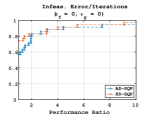
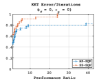
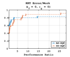
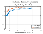
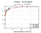
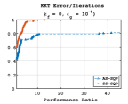
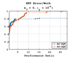
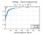
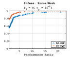
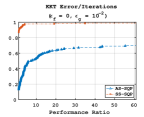
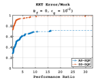
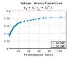
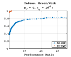
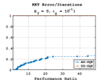
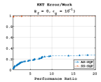
Figure 1: Performance profiles for AS-SQP and SS-SQP on CUTEst collection [18] with deterministic objective function evaluations ($\epsilon_{f}=0$) and noisy objective gradient evaluations. Each column corresponds to a different evaluation metric (infeasibility and KKT errors vs. iterations and work). The noise in the objective gradient evaluations $\epsilon_{g}$ increases from top to bottom (First row: $\epsilon_{g}=0$; Second row: $\epsilon_{g}=10^{-4}$; Third row: $\epsilon_{g}=10^{-2}$; Fourth row: $\epsilon_{g}=10^{-1}$).

4.5 Noisy Functions and Gradients

Here we present results with noise in both the objective function and gradient evaluations. As in Figure 1, in Figure 2 different rows show results for different noise levels in the gradient (the bottom row has the highest noise) and different columns show results for different evaluation metrics. Each performance profile has 4 lines: the AS-SQP (that is objective-function-free and is not affected by the noise in the function evaluations) and three variants of the SS-SQP method with different levels of noise in the objective function evaluations. One can make the following observations. First, not surprisingly, the performance of the SS-SQP method degrades as the noise in the objective function evaluations increases. Second, AS-SQP and SS-SQP are competitive and achieve similar robustness levels with respect to infeasibility errors. Third, and most interestingly, the performance of the methods depends on the relative errors of the function and gradient evaluations. In particular, when the objective function noise level is sufficiently small compared to the objective gradient bias, SS-SQP performs better. On the other hand, when the function estimations are too noisy compared to the noise level in the gradient evaluations, AS-SQP performs slightly better. These results highlight the power of objective-function-free optimization methods in the presence of noise (especially high noise in the objective function evaluations) and the value of quality (or at least relative quality) function evaluations in methods that require zeroth-order information.

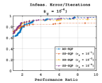
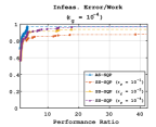
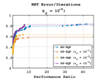
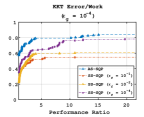
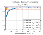
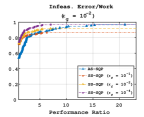
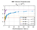
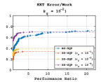
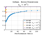
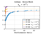
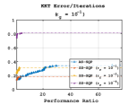
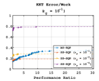
Figure 2: Performance profiles for AS-SQP and SS-SQP on CUTEst collection [18] with noise in both the objective function and gradient evaluations. Each column corresponds to a different evaluation metric (infeasibility and KKT vs. iterations and work). The noise in the objective gradient evaluations $\epsilon_{g}$ increases from top to bottom (First row: $\epsilon_{g}=10^{-4}$; Second row: $\epsilon_{g}=10^{-2}$; Third row: $\epsilon_{g}=10^{-1}$). The different variants of SS-SQP correspond to different levels of noise in the objective function evaluations.

5 Conclusion

We have proposed a step-search SQP algorithm (SS-SQP) for solving stochastic optimization problems with deterministic equality constraints, i.e., the setting in which constraint function values and derivatives are available, but only stochastic estimates of the objective function and its associated derivatives can be computed. We showed that under reasonable assumptions on the inexact probabilistic zeroth- and first-order oracles, with overwhelmingly high probability, in $O(\varepsilon^{-2})$ iterations our algorithm can produce an iterate that satisfies the first-order $\varepsilon$-stationarity, which matches the iteration complexity of the deterministic counterparts of the SQP algorithm [16]. Numerical results provide strong evidence for the efficiency and efficacy of the proposed method. Some future directions include but are not limited to, $(1)$ incorporating stochastic constraint evaluations into the algorithm design and analysis, and $(2)$ extending the framework to the setting with inequality constraints. Both avenues above are subjects of future work as they require significant adaptations in the design, analysis, and implementation of the algorithm.

References

- [1] Afonso S Bandeira, Katya Scheinberg, and Luis Nunes Vicente. Convergence of trust-region methods based on probabilistic models. SIAM J. Optim., 24(3):1238–1264, 2014.
- [2] Stefania Bellavia, Eugenio Fabrizi, and Benedetta Morini. Linesearch Newton-CG methods for convex optimization with noise. arXiv preprint arXiv:2205.06710, 2022.
- [3] Albert S Berahas, Raghu Bollapragada, and Baoyu Zhou. An adaptive sampling sequential quadratic programming method for equality constrained stochastic optimization. arXiv preprint arXiv:2206.00712, 2022.
- [4] Albert S Berahas, Richard H Byrd, and Jorge Nocedal. Derivative-free optimization of noisy functions via quasi-Newton methods. SIAM J. Optim., 29(2):965–993, 2019.
- [5] Albert S Berahas, Liyuan Cao, and Katya Scheinberg. Global convergence rate analysis of a generic line search algorithm with noise. SIAM J. Optim., 31(2):1489–1518, 2021.
- [6] Albert S Berahas, Frank E Curtis, Michael J O’Neill, and Daniel P Robinson. A stochastic sequential quadratic optimization algorithm for nonlinear equality constrained optimization with rank-deficient jacobians. arXiv preprint arXiv:2106.13015, 2021.
- [7] Albert S Berahas, Frank E Curtis, Daniel Robinson, and Baoyu Zhou. Sequential quadratic optimization for nonlinear equality constrained stochastic optimization. SIAM J. Optim., 31(2):1352–1379, 2021.
- [8] Albert S Berahas, Jiahao Shi, Zihong Yi, and Baoyu Zhou. Accelerating stochastic sequential quadratic programming for equality constrained optimization using predictive variance reduction. arXiv preprint arXiv:2204.04161, 2022.
- [9] Dimitri Bertsekas. Network optimization: continuous and discrete models, volume 8. Athena Scientific, 1998.
- [10] Jose Blanchet, Coralia Cartis, Matt Menickelly, and Katya Scheinberg. Convergence rate analysis of a stochastic trust-region method via supermartingales. INFORMS J. Optim., 1(2):92–119, 2019.
- [11] Richard H Byrd, Frank E Curtis, and Jorge Nocedal. An inexact SQP method for equality constrained optimization. SIAM J. Optim., 19(1):351–369, 2008.
- [12] Liyuan Cao, Albert S Berahas, and Katya Scheinberg. First-and second-order high probability complexity bounds for trust-region methods with noisy oracles. arXiv preprint arXiv:2205.03667, 2022.
- [13] Coralia Cartis and Katya Scheinberg. Global convergence rate analysis of unconstrained optimization methods based on probabilistic models. Math. Program., 169(2):337–375, 2018.
- [14] Changan Chen, Frederick Tung, Naveen Vedula, and Greg Mori. Constraint-aware deep neural network compression. In Proceedings of the ECCV, pages 400–415, 2018.
- [15] Ruobing Chen, Matt Menickelly, and Katya Scheinberg. Stochastic optimization using a trust-region method and random models. Math. Program., 169(2):447–487, 2018.
- [16] Frank E Curtis, Michael J O’Neill, and Daniel P Robinson. Worst-case complexity of an SQP method for nonlinear equality constrained stochastic optimization. arXiv preprint arXiv:2112.14799, 2021.
- [17] Frank E Curtis, Daniel P Robinson, and Baoyu Zhou. Inexact sequential quadratic optimization for minimizing a stochastic objective function subject to deterministic nonlinear equality constraints. arXiv preprint arXiv:2107.03512, 2021.
- [18] Nicholas IM Gould, Dominique Orban, and Philippe L Toint. CUTEst: a constrained and unconstrained testing environment with safe threads for mathematical optimization. Comput. Optim. Appl., 60(3):545–557, 2015.
- [19] Serge Gratton, Clément W Royer, Luís N Vicente, and Zaikun Zhang. Complexity and global rates of trust-region methods based on probabilistic models. IMA J. Numer. Anal., 38(3):1579–1597, 2018.
- [20] Serge Gratton, Clément W Royer, Luís Nunes Vicente, and Zaikun Zhang. Direct search based on probabilistic descent. SIAM J. Optim., 25(3):1515–1541, 2015.
- [21] Elad Hazan and Haipeng Luo. Variance-reduced and projection-free stochastic optimization. In International Conference on Machine Learning, pages 1263–1271. PMLR, 2016.
- [22] Billy Jin, Katya Scheinberg, and Miaolan Xie. High probability complexity bounds for line search based on stochastic oracles. arXiv preprint arXiv:2106.06454, 2021.
- [23] Harold Joseph Kushner and Dean S Clark. Stochastic approximation methods for constrained and unconstrained systems, volume 26. Springer Science & Business Media, 2012.
- [24] Guanghui Lan. First-order and stochastic optimization methods for machine learning. Springer, 2020.
- [25] Haihao Lu and Robert M Freund. Generalized stochastic Frank–Wolfe algorithm with stochastic “substitute” gradient for structured convex optimization. Math. Program., 187(1):317–349, 2021.
- [26] Jorge J Moré and Stefan M Wild. Benchmarking derivative-free optimization algorithms. SIAM J. Optim., 20(1):172–191, 2009.
- [27] Sen Na, Mihai Anitescu, and Mladen Kolar. Inequality constrained stochastic nonlinear optimization via active-set sequential quadratic programming. arXiv preprint arXiv:2109.11502, 2021.
- [28] Sen Na, Mihai Anitescu, and Mladen Kolar. An adaptive stochastic sequential quadratic programming with differentiable exact augmented lagrangians. Math. Program., pages 1–71, 2022.
- [29] Sen Na and Michael W Mahoney. Asymptotic convergence rate and statistical inference for stochastic sequential quadratic programming. arXiv preprint arXiv:2205.13687, 2022.
- [30] Yatin Nandwani, Abhishek Pathak, and Parag Singla. A primal dual formulation for deep learning with constraints. Advances in Neural Information Processing Systems, 32, 2019.
- [31] Jorge Nocedal and Stephen Wright. Numerical optimization. Springer Series in Operations Research and Financial Engineering. Springer-Verlag New York, 2006.
- [32] Figen Oztoprak, Richard Byrd, and Jorge Nocedal. Constrained optimization in the presence of noise. arXiv preprint arXiv:2110.04355, 2021.
- [33] Courtney Paquette and Katya Scheinberg. A stochastic line search method with expected complexity analysis. SIAM J. Optim., 30(1):349–376, 2020.
- [34] Sathya N Ravi, Tuan Dinh, Vishnu Suresh Lokhande, and Vikas Singh. Explicitly imposing constraints in deep networks via conditional gradients gives improved generalization and faster convergence. In Proceedings of the AAAI Conference on Artificial Intelligence, volume 33, pages 4772–4779, 2019.
- [35] Tyrone Rees, H Sue Dollar, and Andrew J Wathen. Optimal solvers for PDE-constrained optimization. SIAM J. Sci. Comput., 32(1):271–298, 2010.
- [36] Lindon Roberts and Clément W Royer. Direct search based on probabilistic descent in reduced spaces. arXiv preprint arXiv:2204.01275, 2022.
- [37] Soumava Kumar Roy, Zakaria Mhammedi, and Mehrtash Harandi. Geometry aware constrained optimization techniques for deep learning. In Proceedings of CVPR, pages 4460–4469, 2018.
- [38] Katya Scheinberg and Miaolan Xie. Stochastic adaptive regularization method with cubics: A high probability complexity bound. In OPT 2022: Optimization for Machine Learning (NeurIPS 2022 Workshop).
- [39] Alexander Shapiro, Darinka Dentcheva, and Andrzej Ruszczynski. Lectures on stochastic programming: modeling and theory. SIAM, 2021.