Bosonization of the interacting Su-Schrieffer-Heeger model

Abstract

We derive the bosonization of the interacting fermionic Su-Schrieffer-Heeger (SSH) with open boundaries. We use the classical Euler-Lagrange equations of motions of the bosonized theory to compute the density profile of the Majorana edge mode and observe excellent agreement with numerical results, notably the localization of the mode near the boundaries. Remarkably, we find that repulsive or attractive interactions do not systematically localize or delocalize the edge mode but their effects depend on the value of the staggering parameter. We provide quantitative predictions of these effects on the localization length of the edge mode.

Topological concepts have become a central part of contemporary condensed matter physics [1]. The understanding of the geometrical and topological objects underpinning band theory [2, 3, 4, 5] has fostered intense activities in diverse areas of condensed matter physics such as the study of the quantum Hall effect [6, 7], spin-orbit induced topological band insulators [8, 9, 10], topological quantum computing [11] and so on and so forth.

One current limitation of topological band theory is its restriction to non-interacting systems. Interactions will in general spoil the band structure, rendering usual classification schemes inoperative. There, novel phenomena may be expected, the most famous example being the fractional quantum Hall effect [12].

One of the simplest model capturing the key features of topological insulators is the Su-Shrieffer-Heeger (SSH) model [13]. The fermionic SSH model consists of a 1D tight-binding model with alternating bond value. Depending on whether the first bond is weak (strong) the model is either in the topological (trivial) phase. For open boundaries, one possible characterization of the topological phase is the presence of two-fold, quasi-degenerate, zero energy, Majorana edge modes that are exponentially localized at the boundaries. Remarkably, these edge modes have been observed and characterized experimentally in one-dimensional optical lattices [14] and artificial spin chains simulated with Rydberg atoms [15] in ultracold atoms setup.

Although the SSH is now considered a textbook model for topological insulators, the inclusion of interactions in this model remains to this day an open question. On the other hand, a powerful technique that was developped in the previous decades to treat interacting fermionic systems in 1D is bosonization [16, 17]. One trademark prowess of bosonization is to map interacting spinless fermions in 1D to a free bosonic theory. Remarkably this technique has been successfully applied to study the effects of interactions on Majorana modes in superconducting wires [18, 19, 20] but so far, to the best of our knowledge, the SSH model has escaped from a similar treatment. In particular, the spatial localization of the edge modes has not been described within the bosonization language.

In this paper, we fill this gap by deriving the bosonized theory of the interacting SSH model with open boundaries. We use the classical Euler-Lagrange (EL) equations of motion of the bosonized theory to compute the density profile of the Majorana edge mode and observe excellent agreement with numerical results, notably the localization of the mode near the boundaries. Remarkably, we find that repulsive or attractive interactions do not systematically localize or delocalize the edge mode but their effects depend on the value of the staggering parameter. We provide quantitative predictions of these effects on the localization length. Our results pave the way to a generalization to other interacting topological models.

We begin by discussing the bosonization procedure in the absence of interactions. Let $(c_{j},c_{j}^{\dagger})_{j\in[1,N]}$ be the usual fermionic creation and annihilation operators associated to site $j$. The discrete free SSH Hamiltonian on $N$ sites in 1D is given by

$$H=\sum_{j=1}^{N-1}\left(-t-\delta(-1)^{j}\right)\left(c_{j}^{\dagger}c_{j+1}+{\rm h.c}\right),$$ (1)

i.e we have a tight binding chain with alternating values for the bond. Fixing $t>0$, the topological phase corresponds to the case where we have an even number of sites and $\delta>0$. A signature of the topological phase is the existence for open conditions of quasi-degenerate zero energy eigenstates in which a single particle is in a coherent superposition between the two edges of the chain - see e.g [22, 23] for details on the non-interacting case.

The Fourier transform for open boundaries is given by

$$c_{j}=i\sqrt{\frac{2}{N+1}}\sum_{n=1}^{N}\tilde{c}_{n}\sin\left(\frac{\pi jn}{N+1}\right).$$ (2)

For $\delta=0$, this rotation diagonalizes the problem, i.e we have $H_{\delta=0}=\sum_{n}\varepsilon_{n}\tilde{c}_{n}^{\dagger}\tilde{c}_{n}$ with $\varepsilon_{n}\equiv-2t\cos\left(\frac{\pi n}{N+1}\right)$.

The continuum limit is obtained by introducing the lattice spacing $a$ and defining the position $x\equiv ja$ and the momentum $k\equiv\frac{2\pi n}{2a(N+1)}$. The size of the sytem is taken to be $L\equiv a(N+1)$ so that $k=\frac{\pi n}{L}$. The continuous fermionic field is $\Psi(x)\equiv\frac{1}{\sqrt{a}}c_{j}$. The boundary conditions for $\Psi$ are obtained by extending the discrete formula (2) to site $0$ and site $N+1$ : $\Psi(0)=0$ and $\Psi(x=a(N+1)=L)=0$.

Following the usual bosonization procedure [17, 24], we split $\Psi$ into a left and a right moving fields $\Psi_{{\rm R/L}}$ by expanding around the Fermi energy $\varepsilon_{k_{F}}$:

$$\Psi(x) =\Psi_{{\rm R}}(x)+\Psi_{{\rm L}}(x),$$ (3)

$$\Psi_{{\rm R}}(x) =\sqrt{\frac{L}{2}}e^{ik_{F}x}\int_{-\infty}^{\infty}\frac{dk}{\pi}\tilde{c}_{k+k_{F}}e^{ikx},$$ (4)

$$\Psi_{{\rm L}}(x) =-\Psi_{{\rm R}}(-x).$$ (5)

For convenience, we also define the “slow” fields ${\rm R}(x)\equiv\Psi_{{\rm R}}(x)e^{-ik_{F}x},\quad{\rm L}(x)\equiv e^{ik_{F}x}\Psi_{{\rm L}}(x).$ Importantly, because of open boundaries, the left and right movers are not independent as is encapsulated by Eq.(2), see e.g [25, 26, 27] for previous discussions of open boudaries bosonization.

In the continuum, ${\rm R}(x)$ taken alone can be thought of as a field living on a space of size $2L$ with periodic boundary conditions. In the bosonized language, it can then be reexpressed as

$${\rm R}(x) =F_{{\rm R}}\frac{1}{\sqrt{2\pi\alpha}}e^{i\phi^{R}(x)},$$ (6)

$$\phi^{{\rm R}}(x) \equiv\frac{\pi x}{L}N_{{\rm R}}+\sum_{n>0}\frac{1}{\sqrt{n}}(a_{n}e^{i\frac{n\pi x}{L}}+a_{n}^{\dagger}e^{-i\frac{n\pi x}{L}})e^{-\alpha\frac{\pi n}{2L}}.$$ (7)

where $F_{{\rm R}}$ is the Klein factor associated to the right-mover with $F_{{\rm R}}^{\dagger}F_{{\rm R}}=F_{{\rm R}}F_{{\rm R}}^{\dagger}=1$, $N_{{\rm R}}$ the particle number operator associated to the right movers, $(a_{n},a_{n}^{\dagger})_{n>0}$ a set of bosonic modes indexed by $n$ and $\alpha$ a regularization parameter. The expression of the bosonic field associated to the left-movers can be readily deduced from (5). $F_{{\rm L}}=-F_{{\rm R}}$, $\phi^{{\rm L}}(x)=\phi^{{\rm R}}(-x)$. The conjugated fields $\phi$, $\theta$ are customarily defined as

$$\phi(x) \equiv\frac{-\phi_{R}(x)+\phi_{L}(x)}{2},$$

$$=-\frac{\pi x}{L}N_{R}-i\sum_{n>0}\frac{1}{\sqrt{n}}(a_{n}-a_{n}^{\dagger})\sin\left(\frac{n\pi x}{L}\right)e^{-\alpha\frac{\pi n}{2L}},$$ (8)

$$\theta(x) \equiv\frac{\phi_{R}(x)+\phi_{L}(x)}{2},$$

$$=\sum_{n>0}\frac{1}{\sqrt{n}}(a_{n}+a_{n}^{\dagger})\cos\left(\frac{n\pi x}{L}\right)e^{-\alpha\frac{\pi n}{2L}}.$$ (9)

The particle density operator $\rho$, which counts the number of particle above the Fermi sea, is deduced from $\phi(x)$ through the relation

$$\rho(x)=-\frac{1}{\pi}\partial_{x}\phi(x).$$ (10)

In the remaining, as we want to characterize the $0$ energy modes, we will work at half-filling. It is important to notice that the definition of the half-filling depends on the total number of sites. Let $N_{F}\in\mathbb{N}$ label the last occupied state of the Fermi sea. For $N$ even, we have $N_{F}\equiv\frac{N}{2}$. The corresponding momentum is $k_{F}=\frac{\pi N/2}{a(N+1)}\approx\frac{\pi}{2a}-\frac{\pi}{2aN}\approx\frac{\pi}{2a}-\frac{\pi}{2L}$ to first order in $1/L$. For $N$ odd, the two possible definitions of the half-filled state are $N_{F}=\frac{N\pm 1}{2}$ with corresponding Fermi momenta $k_{F}=\frac{\pi}{2a}-\frac{\pi}{2L}(1\mp 1)$. In the remaining of the paper, we will chose the convention $N_{F}=\frac{N-1}{2}$ for odd number of sites. The Fermi sea state with all modes filled up to $N_{F}$ and empty above will be referred to as the vacuum state.

We show in the SM [28] that $H$ can be expressed in terms of the bosonic fields as

$$H=\int_{0}^{L}dx\bigg{(}\frac{v_{F}}{2\pi}\left(:(\partial_{x}\phi)^{2}:+:(\partial_{x}\theta)^{2}:\right)$$ (11)

$$+\frac{\delta}{L\sin\frac{\pi x}{L}}:\cos\left(2\phi(x)+\left(\frac{\pi}{a}-2k_{F}-\frac{\pi}{L}\right)x\right):\bigg{)}$$

where :: denotes normal-ordering of the fermionic modes with respect to the vacuum and $v_{F}\equiv 2ta\sin(k_{F}a)$ the Fermi velocity. Formula (11) constitutes one of the main results of this paper. We see that the SSH in the bosonized language is almost equivalent to a sine-Gordon Hamiltonian except for the spatial dependence of the prefactor in front of the sinus. To derive (11), we discarded constant terms and fast-varying modes $\propto e^{2ik_{F}x}$, so the bosonic field describes modes with slow spatial variation with respect to the lattice spacing. Since bosonization is a theory describing low energy excitations, we also expect this expression to be valid for $\frac{\delta}{t}\ll 1$.

We now turn to the computation of $\rho$ using the classical Euler-Lagrange (EL) equations of motion. Let $Z\equiv{\rm tr}(e^{-\beta H})$ and $\Pi$ the conjugated field to $\phi$, $\Pi\equiv\frac{1}{\pi}\partial_{x}\theta.$ In the imaginary time formalism, we have

$$Z =\int{\cal D}\phi{\cal D}\Pi e^{\int_{0}^{\beta}\int_{0}^{L}d\tau dx{\cal L}},$$ (12)

with ${\cal L}$ the Lagrangian density : $\int dx{\cal L}=\int dxi\Pi\partial_{\tau}\phi-H$.

The EL equations $\frac{\partial{\cal L}}{\partial\phi}=\frac{\partial}{\partial\tau}\frac{\partial{\cal L}}{\partial\partial_{\tau}\phi}+\frac{\partial}{\partial x}\frac{\partial{\cal L}}{\partial\partial_{x}\phi}$ yields

$$\frac{1}{v_{F}}\partial_{\tau}^{2}\phi+v_{F}\partial_{x}^{2}\phi$$

$$=-\frac{2\pi\delta}{L\sin\frac{\pi x}{L}}\sin\left(2\phi(x)+\left(\frac{\pi}{a}-2k_{F}-\frac{\pi}{L}\right)x\right).$$ (13)

In the $0$ temperature limit, all the weight of the probability measure will be contained in the stationary solution $\partial_{\tau}\phi=0$. Introducing the natural rescaling $y\equiv x/L$, $\varphi(y)\equiv\phi(yL)$, we get the $L$-independent equation

$$\partial_{y}^{2}\varphi(y) =-\Delta\frac{\sin(2\varphi(y)+\epsilon\pi y)}{\sin(\pi y)}.$$ (14)

where we introduced $\Delta=\frac{2\pi\delta L}{v_{F}}\approx\frac{\pi\delta(N+1)}{t}$ and $\epsilon=0$, for an even number of sites where $k_{F}=\frac{\pi}{2a}-\frac{\pi}{2L}$ and $\epsilon=1$ for an odd number of sites using the convention $k_{F}=\frac{\pi}{2a}-\frac{\pi}{L}$. The boundary conditions for $\varphi$ are read from Eq.(8): At $y=0$ we have $\varphi=0$ and at $y=1$ we have $\varphi=-\pi n_{{\rm R}}$ with $n_{{\rm R}}$ the number of particles created on top of the vacuum.

Let us make some remarks here. First, note that $\Delta$ is an adimensioned parameter that fully characterizes the solution of the EL equations. Note that $\Delta$ scales linearly in $N$ and $\frac{\delta}{t}$, so increasing the system size has exactly the same effect as increasing the ratio $\frac{\delta}{t}$. Interestingly, going from the odd to the even case is equivalent to shift $\varphi$ by $\frac{\pi}{2}y$ which can be interpreted as substracting half a particle to the system.

To the best of our knowledge, (14) has no known analytical solution and we have to resort to numerics. To assert the validity of our approach, we compare numerical solutions of (14) with exact diagonalization (ED) results performed on the discrete Hamiltonian (1) in the zero temperature ground state. The ED results show fast oscillations on the scale of the lattice spacing $\propto 1/k_{F}$ that we do not see from the solutions of the EL equations of motion since we precisely discarded these terms. Coarse-graining over the fast oscillations gives a smoothly varying density profile on the scale of the total system size. We observe excellent agreement between the ED and the EL solutions - see Fig.1. We also checked that the agreement holds both for $\delta$ positive or negative, for an even or an odd number of sites and for different values of $n_{{\rm R}}$ [28].

For the even case and $n_{R}=0$ the solution of the EL equations is simply $\phi=0$ so that $\rho(x)=0$, which is consistent with the particle-hole symmetry of the model. For $\delta>0$, fixing $n_{R}=1$ amounts to populate the first mode above the vacuum state, i.e the Majorana edge mode. From (10,14), we can thus deduce the density profile of this edge mode. We plot on Fig.1 the numerical solution of (14) and indeed see a concentration of the density at the boundaries. There is a nice interpretation from Eq.(11). The term proportional to $\delta$ wants to lock the field in the minima of the $\cos$ term. For $N$ even and $\delta>0$, this corresponds to $\phi=-\frac{\pi}{2}[\pi]$. To match the boundary condition, the field $\phi$ must jump from $0$ to $-\pi/2$ and then from $-\pi/2$ to $-\pi$. These jumps translates in concentration on the edges for the density $\rho(x)=-\frac{1}{\pi}\partial_{x}\phi(x)$. The stiffness of the jumps of $\phi$ is controlled by $\Delta$ and determines how much the mode is concentrated at the edges. Eq.(14) is consistent with the exponential localization of the edge mode near the boundary. Indeed, for small $y$, one crude approximation of Eq.(14) at first order in $y$ is given by $\partial_{y}(\partial_{y}\varphi)\approx-\frac{2\Delta}{\pi}\partial_{y}\varphi$. Using additionally that the total particle number is 1, i.e $\frac{1}{\pi}\int_{0}^{1}dy\partial_{y}\varphi(y)=1$, leads to the following ansatz $\varphi_{{\rm A}}$ when $\Delta\gg 1$ :

$$\partial_{y}\varphi_{{\rm A}}(y) =-\Delta\frac{\cosh(\frac{\Delta}{\pi}(2y-1))}{\sinh(\frac{\Delta}{\pi})}.$$ (15)

This exponential ansatz dictates the expression for the typical localization length of the edge mode

$$\ell\equiv\frac{\pi L}{2\Delta}=\frac{v_{F}}{4\delta}.$$ (16)

For the free SSH, it is known -see e.g [22, 23]- that $\ell\propto\frac{a}{\ln\frac{t+\delta}{t-\delta}}\approx\frac{at}{2\delta}$ for $\frac{\delta}{t}\ll 1$, which is consistent with our result since $v_{F}\approx 2ta$ at half-filling. Remark that being in the $\frac{\delta}{t}\ll 1$ regime automatically implies that $\ell\gg a$.

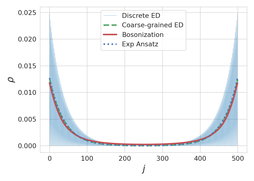
Figure 1: Comparison between the results of the discrete ED, the bosonization result and the exponential fit for $\Delta=20$, $N=500$. The uniform vacuum density $\rho_{j}=1/2$ has been substracted. The light-blue curve corresponds to exact discrete ED result which show fast oscillations at the scale of the lattice spacing. The green dashed curve represents the same data coarse-grained over $2$ sites. The red curve is the density profile obtained by solving the EL equation (14) from the bosonized theory and using $\rho_{j}=\frac{1}{2}-\frac{1}{\pi}\partial_{x}\phi(x=ja)$ and $\phi(x=ja)=\phi^{\prime}(y)$. Lastly, the dashed blue line is obtained from the exponential ansatz (15). Note that the latter two appear superposed on this plot.

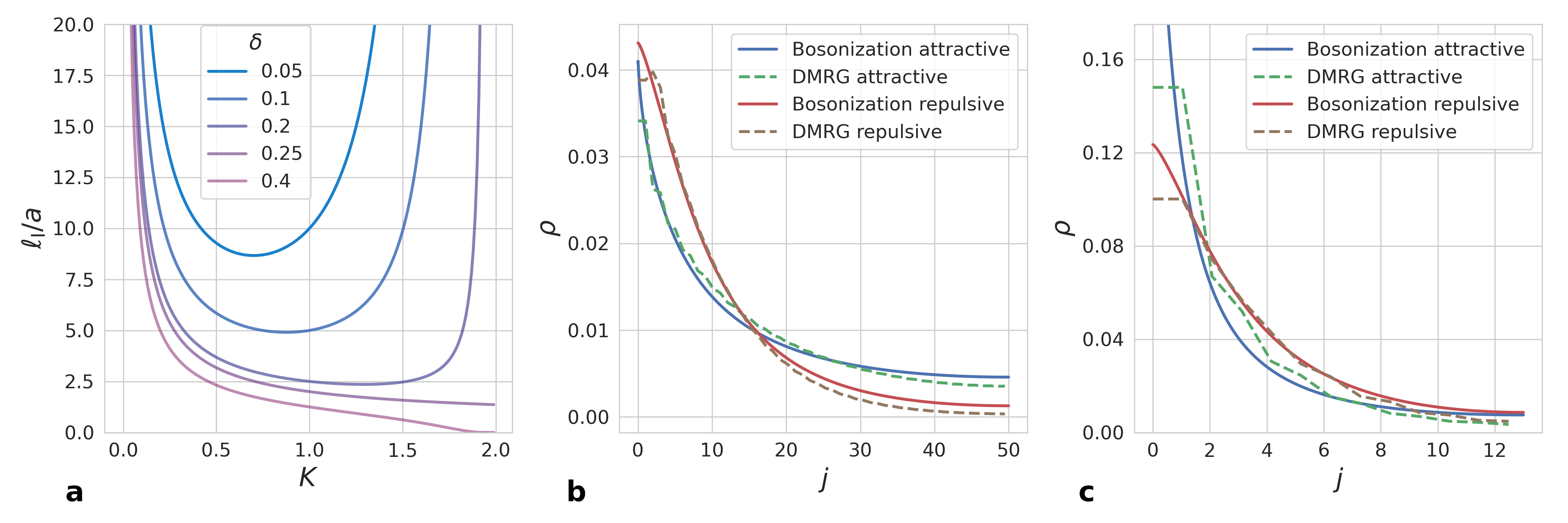
Figure 2: a Plots of relation (22) for the localization length in the interacting case as a function of $K$ for different values of $\delta$. We see that the effect of interactions on the edge mode strongly depends on the value of $\delta$. b Comparison between the solution of the EL equations of motion (19) in the interacting case with DMRG simulations. The DMRG results for attractive (repulsive) interactions have been coarse-grained once (twice) over two sites. Only half of the solution is shown for better readibility. We took $N=100$, $\delta=0.05$, $V=1.6$, $K=0.7$ for the repulsive case and $V=-0.77$, $K=1.4$ for the attractive case. In this case, attractive (repulsive) interactions delocalize (localize) the edge mode. c Same than b with parameters value $N=26$, $\delta=0.2$, $V=1.6$, $K=0.7$ for the repulsive case and $V=-0.77$, $K=1.4$ for the attractive case. We see that, in comparison to case b, the qualitative effect of interactions are swaped.

We now turn to interactions. We consider a nearest neighbor interacting term of the form

$$H_{{\rm I}}:=V\sum_{j=1}^{N-1}\left(n_{j}-1/2\right)\left(n_{j+1}-1/2\right),$$ (17)

with $n_{j}:=c_{j}^{\dagger}c_{j}$ the particle number operator. From now on, we will work exclusively, in the topological phase, i.e $\delta>0$, $N$ even and $N_{F}=\frac{N}{2}$. We show in the SM [28] that in the presence of this interacting term, the bosonization procedure leads for the total Hamiltonian to

$$H= \int_{0}^{L}dx\Big{(}\frac{1}{2\pi}\left(\frac{u}{K}:(\partial_{x}\phi)^{2}:_{{\rm I}}+uK:(\partial_{x}\theta)^{2}:_{{\rm I}}\right)$$

$$+\delta\left(\frac{2}{a\pi}\right)^{1-K}\frac{1}{\left(L\sin\frac{\pi x}{L}\right)^{K}}:\cos(2\phi):_{{\rm I}}\Big{)}.$$ (18)

With $uK\equiv v_{F}$ and $\frac{u}{K}\equiv v_{F}+\frac{4Va}{\pi}$. Since the free part of the Hamiltonian has been rescaled by interactions, normal ordering needs to be done with respect to the new “squeezed” vacuum which we denote by $::_{{\rm I}}$. The $K$ dependence of the prefactors of the $\cos$ terms is a direct consequence of that. In principle, since we are at half-filling, there should also be a $\cos(4\phi)$ term [28]. For simplification, we will neglect this contribution in the present work as it is irrelevant in the RG sense if the interactions are not too repulsive, i.e if $K>1/2$. Eq. (18) is the second crucial result of the paper. The EL equations of motion in the presence of interactions become

$$\partial_{y}^{2}\varphi(y)=-2\left(\frac{L}{a}\right)^{2}\left(\frac{a\pi}{2L}\right)^{K}K^{2}\frac{\delta}{t}\frac{\sin(2\varphi)}{\left(\sin(\pi y)\right)^{K}}.$$ (19)

A comparison of numerical solutions of (19) and density-matrix renormalization group (DMRG) simulations is shown on Fig.2-b for $\delta=0.05$, $N=100$ and $V=1.6$, $K=1.4$ for the attractive case and $V=-0.77$, $K=1.4$ for the repulsive case. We see that the EL equations of motion predicts the correct density profile. For these parameters, we see that attractive interactions delocalize the edge mode into the bulk while repulsive interaction localize it further.

For $K<2$, we can give an estimation of the localization length by expanding (19) for $y\ll 1$. This gives

$$\partial_{y}^{2}\varphi(y)=-\left(\frac{2L}{a}\right)^{2-K}K^{2}\frac{\delta}{t}\frac{\varphi(y)}{y^{K}}$$ (20)

Imposing $\varphi(y)=0$, the solution to this equation are of the form

$$\phi(x\ll L)=\sqrt{\frac{x}{L}}J_{\frac{1}{|2-K|}}\left(\left(\frac{2x}{a}\right)^{\frac{2-K}{2}}\left(\frac{\delta}{t}\right)^{\frac{1}{2}}\frac{2K}{|2-K|}\right)$$ (21)

where $J_{\alpha}$ is the Bessel function of the first kind - see [28] for the proof. The precise shape of the Bessel function depends on $\alpha$ but, as one can easily verify, the position of the first maximum of $J_{\alpha}$ scales linearly with $\alpha$. Thus, we define the localization length to be the value $\ell_{{\rm I}}$ such that $\varphi(\ell_{{\rm I}})=\frac{2}{|2-K|}$ where the factor $2$ has been put in order to match with the localization length of the free case. Following this definition, we obtain that

$$\ell_{{\rm I}}=\frac{a}{2}\left(\frac{t}{\delta K^{2}}\right)^{\frac{1}{2-K}}.$$ (22)

The localization length diverges at $K=2$ if $\frac{\delta}{t}<\frac{1}{4}$. This gives a rough criteria for having a localized mode in the attractive regime $K>1$. Importantly, note that $\ell_{\rm I}$ is not, in general, a monotonic function of $K$ see Fig-2-a. Interestingly, one consequence of this is that attractive or repulsive interaction do not systematically delocalize or localize the edge mode, their effect can change depending on the value of $\delta$. This is illustrated on Fig.2-c where we took $\delta=0.2$. Contrary to the previous case shown on Fig.2-b , we see that the effects of attractive interactions is to localize the edge mode further to the boundary and the other way around for the repulsive ones.

Conclusion - In this paper, we derived the bosonized theory of the interacting SSH model with open boundaries. Importantly, our study offers quantitative arguments to determine the effects of interactions on the edge mode and pave the way to study other interacting topological models such as the spin 1 antiferromagnetic Heisenberg chain [29, 30], the AKLT model [31] or the Kitaev fermionic chain [32]. One of our remarkable results for the SSH model is that attractive (repulsive) interactions do not systematically delocalize or localize the edge mode, but this behavior is strongly dependent on the value of the staggering parameter $\delta$.

We focused on the mean density profile of the edge mode but it would be interesting as a future direction to understand the interplay between interactions and quantum correlations of the edges. Another notable point is that we systematically discarded the Umklapp term in our study. Nevertheless, in the strongly repulsive regime, it is expected to play a role, leading to possibly interesting new phenomena.

Supplemental Material

Appendix A Abacus

For the reader’s convenience, we first recall the expression of the fermionic fields in terms of bosonic modes as well as various useful relations they satisfy.

The continuous fermionic field $\Psi$ is split between a right-moving field and a left-moving one :

$$\Psi(x) =\Psi_{{\rm R}}(x)+\Psi_{{\rm L}}(x),$$ (23)

$$\Psi_{{\rm R}}(x) =\sqrt{\frac{L}{2}}e^{ik_{F}x}\int_{-\infty}^{\infty}\frac{dk}{\pi}\tilde{c}_{k+k_{F}}e^{ikx},$$ (24)

$$\Psi_{{\rm L}}(x) =-\Psi_{{\rm R}}(-x).$$ (25)

The main difference with bosonization on an infinite system size is that the left mover is defined from the right mover for open boundaries. The slow-mode is defined as

$${\rm R}(x) \equiv F_{{\rm R}}\frac{1}{\sqrt{2\pi\alpha}}e^{i\phi^{{\rm R}}(x)},$$ (26)

$$\phi^{{\rm R}}(x) \equiv\frac{\pi x}{L}N_{{\rm R}}+\sum_{n>0}\frac{1}{\sqrt{n}}(a_{n}e^{i\frac{n\pi x}{L}}+a_{n}^{\dagger}e^{-i\frac{n\pi x}{L}})e^{-\alpha\frac{\pi n}{2L}}.$$ (27)

One key observation is that ${\rm R}(x)$ can be interpreted as a field with periodic boundary conditions on a system with size $2L$.

The corresponding left mode is

$${\rm L}(x) =F_{{\rm L}}\frac{1}{\sqrt{2\pi\alpha}}e^{i\phi^{{\rm L}}(x)},$$ (28)

$$F_{{\rm L}} =-F_{{\rm R}},$$ (29)

$$\phi^{{\rm L}}(x) =-\frac{\pi x}{L}N_{{\rm R}}+\sum_{n>0}\frac{1}{\sqrt{n}}(a_{n}e^{-i\frac{n\pi x}{L}}+a_{n}^{\dagger}e^{i\frac{n\pi x}{L}})e^{-\alpha\frac{\pi n}{2L}}.$$ (30)

and the canonical fields $\phi$ and $\theta$ are defined as

$$\phi(x) :=\frac{-\phi_{\rm R}(x)+\phi_{\rm L}(x)}{2},$$

$$=-\frac{\pi x}{L}N_{{\rm R}}-i\sum_{n>0}\frac{1}{\sqrt{n}}(a_{n}-a_{n}^{\dagger})\sin\left(\frac{n\pi x}{L}\right)e^{-\alpha\frac{\pi n}{2L}},$$ (31)

$$\theta(x) :=\frac{\phi_{\rm R}(x)+\phi_{\rm L}(x)}{2},$$

$$=\sum_{n>0}\frac{1}{\sqrt{n}}(a_{n}+a_{n}^{\dagger})\cos\left(\frac{n\pi x}{L}\right)e^{-\alpha\frac{\pi n}{2L}}.$$ (32)

It will turn out to be useful to divide the $\phi^{{\rm R}}$ operator into an annihilation part $\varphi^{{\rm R}}$ and a creation part with respect to the vacuum state :

$$\phi^{{\rm R}} =\varphi^{{\rm R}}+\varphi^{{\rm R}\dagger},$$ (33)

$$\varphi^{{\rm R}} =\frac{\pi x}{L}N_{R}+\sum_{n>0}\frac{1}{\sqrt{n}}a_{n}e^{i\frac{n\pi x}{L}}e^{-\alpha\frac{\pi n}{2L}},$$ (34)

$$\varphi^{{\rm R}\dagger} =\sum_{n>0}\frac{1}{\sqrt{n}}a_{n}^{\dagger}e^{-i\frac{2n\pi x}{2L}}e^{-\alpha\frac{\pi n}{2L}}.$$ (35)

These operators have commutation relation

$$[\varphi^{R},\varphi^{R\dagger}] =-\log(1-e^{-\alpha\frac{\pi}{L}}).$$ (36)

Using Baker-Campbell-Hausdorff relation $e^{A+B}=e^{A}e^{B}e^{-\frac{1}{2}[A,B]}$ when $[[A,B],B]=[[A,B],A]=0$ and $e^{-\frac{1}{2}[\varphi^{R},\varphi^{R\dagger}]}=\sqrt{1-e^{-\alpha\frac{\pi}{L}}}\approx\sqrt{\frac{\alpha\pi}{L}}$, we can express $\mathrm{R}(x)$ in terms of normal-ordered operators (Normal-ordering denoted by $::$ here refers to the normal order of bosons with respect to the Fermi sea vacuum state denoted $\left|\Omega\right\rangle$) :

$${\rm R}(x)=F_{\mathrm{R}}\frac{1}{\sqrt{2L}}:e^{i\phi^{\mathrm{R}}(x)}:.$$ (37)

The normal ordered version of the left field is

$${\rm L}(x)=-F_{\mathrm{R}}\frac{1}{\sqrt{2L}}:e^{i\phi^{\mathrm{R}}(-x)}:.$$ (38)

A useful relation allowing us to deal with product of normal ordered field is

$$:e^{ia\phi^{\mathrm{R}}(x)}::e^{ib\phi^{\mathrm{R}}(y)}:=e^{-ab\left\langle\Omega\right|\phi^{\mathrm{R}}(x)\phi^{\mathrm{R}}(y)\left|\Omega\right\rangle}:e^{ia\phi^{\mathrm{R}}(x)+ib\phi^{\mathrm{R}}(y)}:$$ (39)

and an explicit calculation gets us

$$e^{-ab\left\langle\Omega\right|\phi^{\mathrm{R}}(x)\phi^{\mathrm{R}}(y)\left|\Omega\right\rangle}=(1-e^{-\frac{\pi}{L}(\alpha+i(y-x))})^{ab}.$$ (40)

Similarly, for the field $\phi$ :

$$:e^{ia\phi(x)}::e^{ib\phi(y)}:=:e^{ia\phi(x)+ib\phi(y)}:\left(\frac{\sin^{2}\left(\frac{\pi(x+y)}{2L}\right)}{\sin^{2}\left(\frac{\pi(x-y)}{2L}\right)}\right)^{-ab/4}.$$ (41)

Finally, another useful relation for normal-ordering is :

$$e^{ib\phi(x)} =:e^{ib\phi(x)}:e^{-\frac{b^{2}}{2}\left\langle\Omega\right|\phi^{2}(x)\left|\Omega\right\rangle},$$ (42)

$$=:e^{ib\phi(x)}:\left(\frac{2L}{\pi\alpha}\sin\left(\frac{\pi x}{L}\right)\right)^{-\frac{b^{2}}{4}}.$$ (43)

Appendix B Derivation of the bosonized form of the SSH Hamiltonian

In this part, we show how to derive the bosonized Hamiltonians (11) and (18) of the main text.

The discrete Hamiltonian of the fermionic interacting SSH with open boundaries was given by

$$H=\sum_{j=1}^{N-1}\left(-t-\delta(-1)^{j}\right)\left(c_{j}^{\dagger}c_{j+1}+{\rm h.c}\right)+V\left(n_{j}-\frac{1}{2}\right)\left(n_{j+1}-\frac{1}{2}\right).$$ (44)

We split it in three parts that we will treat separately. $H=H_{0}+H_{1}+H_{{\rm I}}$ with $H_{0}$ the tight-binding term, $H_{1}$ the staggered part and $H_{{\rm I}}$ the interacting part

$$H_{0} =-t\sum_{j=1}^{N-1}\left(c_{j}^{\dagger}c_{j+1}+{\rm h.c}.\right),$$ (45)

$$H_{1} =-\delta(-1)^{j}\sum_{j=1}^{N-1}\left(c_{j}^{\dagger}c_{j+1}+{\rm h.c}.\right),$$ (46)

$$H_{{\rm I}} =V\sum_{j=1}^{N-1}\left(n_{j}-\frac{1}{2}\right)\left(n_{j+1}-\frac{1}{2}\right).$$ (47)

B.1 Bosonization of the tight-binding part $H_{0}$

Although the bosonization of the tight-binding chain is a standard textbook derivation, we redo it here because we are dealing with open boundaries. Because of this, the left and right movers are not independent fields and this may give rise to differences with the standard infinite system case.

Let us write $H_{0}$ in terms of the continuous fermionic field :

$$H_{0} =-t\sum_{j=1}^{N-1}\left(c_{j}^{\dagger}c_{j+1}+{\rm h.c}.\right)$$ (48)

$$=-t\int_{0}^{L}dx\left(\Psi^{\dagger}(x)\Psi(x+a)+{\rm h.c}\right),$$ (49)

$$\approx-\frac{t}{2}\int_{-L}^{L}dx\left(e^{ik_{F}a}\mathrm{R}^{\dagger}(x)\mathrm{R}(x+a)+e^{-ik_{F}a}\mathrm{L}^{\dagger}(x)\mathrm{L}(x+a)+{\rm h.c}\right)$$ (50)

where going from the second line to the third we “unfolded” the fields on $[-L,L]$ by making use of ${\rm R}(x)=-{\rm L}(-x)$ and discarded fast oscillating terms proportional to $e^{\pm i2k_{F}x}$, $\Psi_{\mathrm{R}}^{\dagger}\Psi_{\mathrm{L}}$ and $\Psi_{\mathrm{L}}^{\dagger}\Psi_{\mathrm{R}}$. As usual in continuous field theory, the $a\to 0$ limit must be regularized. To this end, we denote by $::\mathrm{R}^{\dagger}(x)\mathrm{R}(x+a)::$ the point-splitting procedure which consists in substracting the infinite vacuum contribution to our operator

$$::\mathrm{R}^{\dagger}(x)\mathrm{R}(x+a):: =\lim_{a\to 0}[\mathrm{R}^{\dagger}(x)\mathrm{R}(x+a)-\left\langle\Omega\right|\mathrm{R}^{\dagger}(x)\mathrm{R}(x+a)\left|\Omega\right\rangle].$$ (51)

Using Eq.(39) we get

$$\mathrm{R}^{\dagger}(x)\mathrm{R}(x+a) =\frac{1}{2L}:e^{-i\phi^{\mathrm{R}}(x)+i\phi^{\mathrm{R}}(x+a)}:(1-e^{-\frac{\pi}{L}(\alpha+ia)})^{-1},$$ (52)

$$\left\langle\Omega\right|\mathrm{R}^{\dagger}(x)\mathrm{R}(x+a)\left|\Omega\right\rangle =\frac{1}{2L}(1-e^{-\frac{\pi}{L}(\alpha+ia)})^{-1}.$$ (53)

$$::\mathrm{R}^{\dagger}(x)\mathrm{R}(x+a):: =\frac{1}{2i\pi a}:\left(ia\partial_{x}\phi^{\mathrm{R}}(x)-\frac{1}{2}\left(a\partial_{x}\phi^{\mathrm{R}}(x)\right)^{2}+i\frac{a^{2}}{2}\partial_{x}^{2}\phi^{\mathrm{R}}(x)\right):$$ (54)

Similarly, for the left moving field, we have

$$::\mathrm{L}^{\dagger}(x)\mathrm{L}(x+a):: =\frac{1}{2i\pi a}:\left(ia\partial_{x}\phi^{\mathrm{R}}(-x)+\frac{1}{2}\left(a\partial_{x}\phi^{\mathrm{R}}(-x)\right)^{2}-i\frac{a^{2}}{2}\partial_{x}^{2}\phi^{\mathrm{R}}(-x)\right):$$ (55)

When integrating these fields over $[-L,L]$, using the periodicity of $\phi^{\mathrm{R}}$ on that interval, the terms $\partial_{x}\phi^{\mathrm{R}}$ and $\partial_{x}^{2}\phi^{\mathrm{R}}$ vanish. Now combining with the h.c. we get

$$-\frac{t}{2}\int_{-L}^{L}dx\left(e^{ik_{F}a}::\mathrm{R}^{\dagger}(x)\mathrm{R}(x+a)::+{\rm h.c.}\right) =-i\frac{ta}{8\pi}\int_{-L}^{L}dx\left(e^{ik_{F}a}:\left(\partial_{x}\phi^{\mathrm{R}}(x)\right)^{2}:-e^{-ik_{F}a}:\left(\partial_{x}\phi^{\mathrm{R}}(x)\right)^{2}:\right),$$ (56)

$$=\underbrace{2ta\sin(k_{F}a)}_{=v_{F}}\frac{1}{8\pi}\int_{-L}^{L}dx:\left(\partial_{x}\phi^{\mathrm{R}}(x)\right)^{2}:.$$ (57)

And similarly for the left field

$$-\frac{t}{2}\int_{-L}^{L}dx\left(e^{-ik_{F}a}::\mathrm{L}^{\dagger}(x)\mathrm{L}(x+a)::+{\rm h.c.}\right) =\frac{v_{F}}{8\pi}\int_{-L}^{L}dx:\left(\partial_{x}\phi^{{\rm L}}(x)\right)^{2}:.$$

Using $\phi^{{\rm R}}(x)=\phi^{{\rm L}}(-x)$ we can fold back everything on the interval $[0,L]$. Using additionally that $(\partial_{x}\phi^{{\rm R}})^{2}+(\partial_{x}\phi^{{\rm L}})^{2}=2((\partial_{x}\phi)^{2}+(\partial_{x}\theta)^{2})$, we end up with

$$H_{0}=\int_{0}^{L}dx\frac{v_{F}}{2\pi}\left(:(\partial_{x}\phi)^{2}:+:(\partial_{x}\theta)^{2}:\right).$$ (58)

B.2 Bosonization of the staggered part $H_{1}$.

We now turn to the bosonization of the staggered part $H_{1}$. The philosophy is essentially the same as before except that, because of the $(-1)^{j}$ prefactor, the slow-varying terms are going to be the cross terms $\Psi_{\mathrm{R}}^{\dagger}\Psi_{\mathrm{L}}$ and $\Psi_{\mathrm{L}}^{\dagger}\Psi_{\mathrm{R}}$ and the fast varying ones, that we will discard, $\Psi_{\mathrm{R}}^{\dagger}\Psi_{\mathrm{R}}$ and $\Psi_{\mathrm{L}}^{\dagger}\Psi_{\mathrm{L}}$.

$$H_{1} =-\delta(-1)^{j}\sum_{j=1}^{N-1}\left(c_{j}^{\dagger}c_{j+1}+{\rm h.c}.\right),$$ (59)

$$=-\delta\int_{0}^{L}dxe^{i\frac{\pi x}{a}}\left(\Psi^{\dagger}(x)\Psi(x+a)+{\rm h.c}\right),$$ (60)

$$\approx-\delta\int_{0}^{L}dx\left(e^{i\frac{\pi x}{a}}e^{-i2k_{F}x}e^{-ik_{F}a}{\rm R}^{\dagger}(x){\rm L}(x+a)+e^{-i\frac{\pi x}{a}}e^{2ik_{F}x}e^{ik_{F}a}{\rm L}^{\dagger}(x){\rm R}(x+a)+{\rm h.c}\right)$$ (61)

where going from the second to the third line, we ignored the fast oscillating terms and made use of the fact that $(-1)^{j}=e^{i\frac{\pi x}{a}}=e^{-i\frac{\pi x}{a}}$ for $x=ja$. Since we are half-filling $2k_{F}x\approx\frac{\pi x}{a}$ which will cancel the $(-1)^{j}$ contribution. However, as is discussed in the main text, the expression of $k_{F}$ has subleading correction in $1/L$ depending on the parity of the number of sites. For $N$ even, $k_{F}\approx\frac{\pi}{2a}-\frac{\pi}{2L}$ to first order in $1/L$. For $N$ odd, the two possible Fermi momenta are $k_{F}\approx\frac{\pi}{2a}-\frac{\pi}{2L}(1\mp 1)$ depending on the convention. We will use the convention $k_{F}=\frac{\pi}{2a}$ for odd sites in the following. It is important to keep track of $1/L$ term since $x$ itself ranges from $0$ to $L$. Thus, terms proportional to $x/L$ are in general not negligible in the thermodynamic limit.

To regularize this expression, we again need to consider the point-splitting of $H_{1}$. We focus on the first term :

$$::{\rm R}^{\dagger}(x){\rm L}(x+a):: =\lim_{a\to 0}[{\rm R}^{\dagger}(x){\rm L}(x+a)-\langle{\rm R}^{\dagger}(x){\rm L}(x+a)\rangle],$$ (62)

$${\rm R}^{\dagger}(x){\rm L}(x+a) =-\frac{1}{2L}:e^{-i\phi^{\mathrm{R}}(x)}::e^{i\phi^{\mathrm{R}}(-x-a)}:.$$ (63)

Using Eq.(39) we get

$${\rm R}^{\dagger}(x){\rm L}(x+a) =-\frac{1}{2L}:e^{-i\phi^{\mathrm{R}}(x)+i\phi^{\mathrm{R}}(-x-a)}:(1-e^{-\frac{i\pi(-2x-a)}{L}})^{-1},$$ (64)

$$=-\frac{i}{4L\sin\frac{\pi(x+a/2)}{L}}e^{-\frac{i\pi(x+a/2)}{L}}:e^{2i\phi(x)+ia\partial_{x}\phi^{\mathrm{L}}(x)}:$$ (65)

which in the limit $a\to 0$ becomes

$${\rm R}^{\dagger}(x){\rm L}(x+a) =-\frac{ie^{-\frac{i\pi x}{L}}}{4L\sin\frac{\pi x}{L}}:e^{2i\phi(x)}:$$ (66)

and

$$::{\rm R}^{\dagger}(x){\rm L}(x+a)::=-\frac{ie^{-\frac{i\pi x}{L}}}{4L\sin\frac{\pi x}{L}}(:e^{2i\phi(x)}:-1).$$ (67)

Similarly

$$::{\rm L}^{\dagger}(x){\rm R}(x+a):: =\frac{ie^{\frac{i\pi x}{L}}}{4L\sin\frac{\pi x}{L}}(:e^{-2i\phi(x)}:-1)$$ (68)

which leads to

$$H_{1} =-\delta\int_{0}^{L}dx\frac{1}{4iL\sin\frac{\pi x}{L}}\left(e^{i\left(-k_{F}a+x(\frac{\pi}{a}-2k_{F}-\frac{\pi}{L})\right)}(:e^{2i\phi(x)}:-1)-e^{-i\left(-k_{F}a+x(\frac{\pi}{a}-2k_{F}-\frac{\pi}{L})\right)}(:e^{-2i\phi(x)}:-1)+{\rm h.c}\right),$$ (69)

$$=-\delta\int_{0}^{L}dx\frac{1}{L\sin\frac{\pi x}{L}}\left(:\sin\left(2\phi(x)+(\frac{\pi}{a}-2k_{F}-\frac{\pi}{L})x-k_{F}a\right):-\sin\left((\frac{\pi}{a}-2k_{F}-\frac{\pi}{L})x-k_{F}a\right)\right),$$ (70)

$$=\delta\int_{0}^{L}dx\frac{1}{L\sin\frac{\pi x}{L}}\left(:\cos\left(2\phi(x)+(\frac{\pi}{a}-2k_{F}-\frac{\pi}{L})x\right):-\cos\left((\frac{\pi}{a}-2k_{F}-\frac{\pi}{L})x\right)\right).$$ (71)

In the last line, we simplified the expression by making the approximation $k_{F}a\approx\frac{\pi}{2}$. Note that such approximation cannot be done for the $k_{F}x$ term. The part independent from $\phi(x)$ is precisely the contribution of the vacuum energy. For the rest of the derivation, we will focus on the case of an even number of sites for which $k_{F}=\frac{\pi}{2a}-\frac{\pi}{2L}$ so that

$$H_{1} =\delta\int_{0}^{L}dx\frac{1}{L\sin\frac{\pi x}{L}}\left(:\cos\left(2\phi(x)\right):-1\right).$$ (72)

B.3 Bosonization of the interacting part $H_{{\rm I}}$.

We now derive the bosonization of the interacting term

$$H_{{\rm I}}\equiv V\sum_{j=1}^{N-1}\left(n_{j}-\frac{1}{2}\right)\left(n_{j+1}-\frac{1}{2}\right)$$ (73)

with $n_{j}$ the particle number operator $c_{j}^{\dagger}c_{j}$. Recall

$$c_{j}^{\dagger}c_{j} =a({\rm R}^{\dagger}(x){\rm R}(x)+{\rm L}^{\dagger}(x){\rm L}(x)+{\rm R}^{\dagger}(x){\rm L}(x)e^{-2ik_{F}x}+{\rm L}^{\dagger}(x){\rm R}(x)e^{2ik_{F}x}).$$

The point-split expressions we previously found were

$$::{\rm R}^{\dagger}(x){\rm R}(x)::=\frac{1}{2\pi}\left(:\partial_{x}\phi^{{\rm R}}:\right),$$ (74)

$$::{\rm L}^{\dagger}(x){\rm L}(x)::=-\frac{1}{2\pi}\left(:\partial_{x}\phi^{{\rm L}}:\right),$$ (75)

$$::{\rm R}^{\dagger}(x){\rm L}(x)::=-\frac{i}{4L}\frac{e^{-i\frac{\pi x}{L}}}{\sin\frac{\pi x}{L}}\left(:e^{2i\phi}:-1\right),$$ (76)

$$::{\rm L}^{\dagger}(x){\rm R}(x)::=\frac{i}{4L}\frac{e^{i\frac{\pi x}{L}}}{\sin\frac{\pi x}{L}}\left(:e^{-2i\phi}:-1\right).$$ (77)

So that

$$::{\rm R}^{\dagger}(x){\rm R}(x)::+::{\rm L}^{\dagger}(x){\rm L}(x):: =-\frac{1}{\pi}\partial_{x}\phi,$$ (78)

$$::{\rm R}^{\dagger}(x){\rm L}(x)e^{-2ik_{F}x}::+::{\rm L}^{\dagger}(x){\rm R}(x)e^{2ik_{F}x}:: =\frac{i}{4L}\frac{e^{-i\frac{\pi x}{a}}}{\sin\frac{\pi x}{L}}\left(:e^{2i\phi}:-:e^{-2i\phi}:\right),$$ (79)

$$=-\frac{e^{-i\frac{\pi x}{a}}}{\pi\alpha}\left(\sin(2\phi)\right).$$ (80)

Where we used the formula $e^{ib\phi(x)}=:e^{ib\phi(x)}:\left(\frac{2L}{\pi\alpha}\sin\left(\frac{\pi x}{L}\right)\right)^{-\frac{b^{2}}{4}}$. Thus,

$$H_{{\rm I}}= aV\int_{0}^{L}dx\left(-\frac{1}{\pi}\partial_{x}\phi(x)-\frac{e^{-i\frac{\pi x}{a}}}{\pi\alpha}\left(\sin(2\phi(x))\right)\right)\left(-\frac{1}{\pi}\partial_{x}\phi(x+a)-\frac{e^{-i\frac{\pi(x+a)}{a}}}{\pi\alpha}\left(\sin(2\phi(x+a))\right)\right).$$ (81)

Terms proportional to $e^{\pm ik_{F}x}$ in this product will be discarded as they are oscillating rapidly. We will also discard any constant term whenever they arise and systematically take the limit $a\to 0$ when it is unambiguous. Note that, because we are at half-filling, we have to keep the Umklapp terms proportional to $e^{\pm i4k_{F}x}$.

$$H_{{\rm I}}= aV\int_{0}^{L}dx\left(\frac{1}{\pi^{2}}\left(\partial_{x}\phi\right)^{2}-\frac{1}{(\pi\alpha)^{2}}\left(\sin(2\phi(x))\sin(2\phi(x+a))\right)\right),$$ (82)

$$= aV\int_{0}^{L}dx\left(\frac{1}{\pi^{2}}\left(\partial_{x}\phi\right)^{2}+\frac{1}{2(\pi\alpha)^{2}}\left(\cos(4\phi(x))-\cos(2a\partial_{x}\phi)\right)\right),$$ (83)

$$\approx aV\int_{0}^{L}dx\left(\frac{2}{\pi^{2}}\left(\partial_{x}\phi\right)^{2}+\frac{\cos(4\phi(x))}{2(\pi a)^{2}}\right)$$ (84)

where in the last line we identified the cut-off $\alpha$ and the lattice spacing $a$. The normal-ordered version is

$$H_{{\rm I}}=\int_{0}^{x}dx\left(\frac{2aV}{\pi^{2}}:(\partial_{x}\phi)^{2}:+\frac{V\pi^{2}a^{3}}{2^{5}\left(L\sin\frac{\pi x}{L}\right)^{4}}:\cos(4\phi):\right).$$ (85)

B.4 Putting everything together and normal-ordering with the new vacuum

Putting everything together, we finally arrive for the total Hamiltonian to

$$H=\int_{0}^{L}dx\left(\frac{1}{2\pi}\left(\frac{u}{K}:(\partial_{x}\phi)^{2}:+uK:\left(\partial_{x}\theta\right)^{2}:\right)+\frac{\delta}{L\sin\frac{\pi x}{L}}:\cos(2\phi):+\frac{V\pi^{2}a^{3}}{2^{5}\left(L\sin\frac{\pi x}{L}\right)^{4}}:\cos(4\phi):\right),$$ (86)

with $uK\equiv v_{F}$ and $\frac{u}{K}=v_{F}+\frac{4Va}{\pi}$. The non-normal ordered version is

$$H=\int_{0}^{L}dx\left(\frac{1}{2\pi}\left(\frac{u}{K}(\partial_{x}\phi)^{2}+uK\left(\partial_{x}\theta\right)^{2}\right)+\frac{2\delta}{a\pi}\cos(2\phi)+\frac{V}{2a\pi^{2}}\cos(4\phi)\right).$$ (87)

With the interactions, the free part of the Hamiltonian has been renormalized. We have to redefine the normal-ordering with respect to this new free Hamiltonian in order to get the correct path integral formulation. Let’s call the new normal order $::_{{\rm I}}$. We introduce the rescaled fields $\tilde{\phi}=\sqrt{K}\phi$ and $\tilde{\theta}=\frac{1}{\sqrt{K}}\theta$. This transformation preserves the commutation relation between the field operators. The free part of the Hamiltonian in terms of these fields is expressed as

$$\int_{0}^{L}\frac{dx}{2\pi}u\left((\partial_{x}\tilde{\phi})^{2}+(\partial_{x}\tilde{\theta})^{2}\right).$$ (88)

We see that it has the same form than a genuine free Hamiltonian whose Fermi velocity would be given by $u$. In particular, let $\left|\Omega_{{\rm I}}\right\rangle$ be the new vacuum. We have :

$$\left\langle\Omega_{{\rm I}}\right|\tilde{\phi}^{2}\left|\Omega_{{\rm I}}\right\rangle=\left\langle\Omega\right|\phi^{2}\left|\Omega\right\rangle=\frac{1}{2}\log\left(\frac{2L}{\pi\alpha}\sin(\frac{\pi x}{L})\right),$$ (89)

so that

$$e^{i\zeta\phi} =:e^{i\zeta\phi}:_{{\rm I}}e^{-\frac{\zeta^{2}}{2}K\left\langle\Omega_{{\rm I}}\right|\tilde{\phi}^{2}\left|\Omega_{{\rm I}}\right\rangle},$$ (90)

$$=:e^{i\zeta\phi}:_{{\rm I}}\left(\frac{2L}{\pi\alpha}\sin(\frac{\pi x}{L})\right)^{-\frac{K\zeta^{2}}{4}}.$$ (91)

The normal-ordered Hamiltonian thus becomes :

$$H= \int_{0}^{L}dx\Bigg{(}\frac{1}{2\pi}\left(\frac{u}{K}:(\partial_{x}\phi)^{2}:_{{\rm I}}+uK:(\partial_{x}\theta)^{2}:_{{\rm I}}\right)+\frac{2\delta}{a\pi}\left(\frac{\pi a}{2}\right)^{K}\frac{1}{\left(L\sin\frac{\pi x}{L}\right)^{K}}:\cos(2\phi):_{{\rm I}}$$ (92)

$$+\frac{V}{2a\pi^{2}}\frac{1}{\left(\frac{2L}{\pi\alpha}\sin(\frac{\pi x}{L})\right)^{4K}}:\cos(4\phi):_{{\rm I}}\Bigg{)}.$$ (93)

Note that in the main text, we neglected the Umklapp contribution which is the $\cos(4\phi)$ term.

Appendix C Bessel functions

In this section, we show that the differential equation

$$\partial_{x}^{2}h=-a\frac{h}{x^{b}}$$ (94)

with $a,b$ real and positive admits as solution functions of the form

$$h(x)\equiv\sqrt{x}f_{(|2-b|)^{-1}}\left(\sqrt{a}\frac{2}{|2-b|}x^{\frac{2-b}{2}}\right)$$ (95)

where $f_{\alpha}$ is a Bessel function of the first or second kind, i.e a function satisfying the following relation :

$$y^{2}f^{\prime\prime}_{\alpha}(y)+yf^{\prime}_{\alpha}(y)+(y^{2}-\alpha^{2})f_{\alpha}(y)=0.$$ (96)

Let $y=\mu x^{\nu}$ and $h(x)=\sqrt{x}f\left(y=\mu x^{\nu}\right)$ with $\mu\geq 0$ and $\nu$ free variables for now. The previous equation translates for $h$ into the relation

$$h(x)x^{-1/2}\left(\frac{1}{4\nu^{2}}-\alpha^{2}\right)+\frac{1}{\nu^{2}}h^{\prime\prime}(x)x^{3/2}+\mu^{2}x^{2\nu-1/2}h(x) =0.$$ (97)

Fixing $\alpha=\frac{1}{|2\nu|}$, we end up with

$$h^{\prime\prime}(x) =-\nu^{2}\mu^{2}x^{2(\nu-1)}h(x).$$ (98)

For $h$ to be solution of (94), we must have

$$\nu =\frac{2-b}{2},$$ (99)

$$|\mu| =\sqrt{a}\frac{2}{|2-b|}$$ (100)

which ends our proof.

Appendix D Additional plots for the free case

For the reader’s convenience, we provide in this section additional plots of the numerical solution of Eq.(14) of the main text as well as comparison with ED result. We vary the sign of $\delta$ to go from the topological to the trivial phase, the parity of the number of sites $N$ and the number of excitations $n_{{\rm R}}$. For each plot, we substracted the average particle number occupation of the vacuum mode for the ED plots.

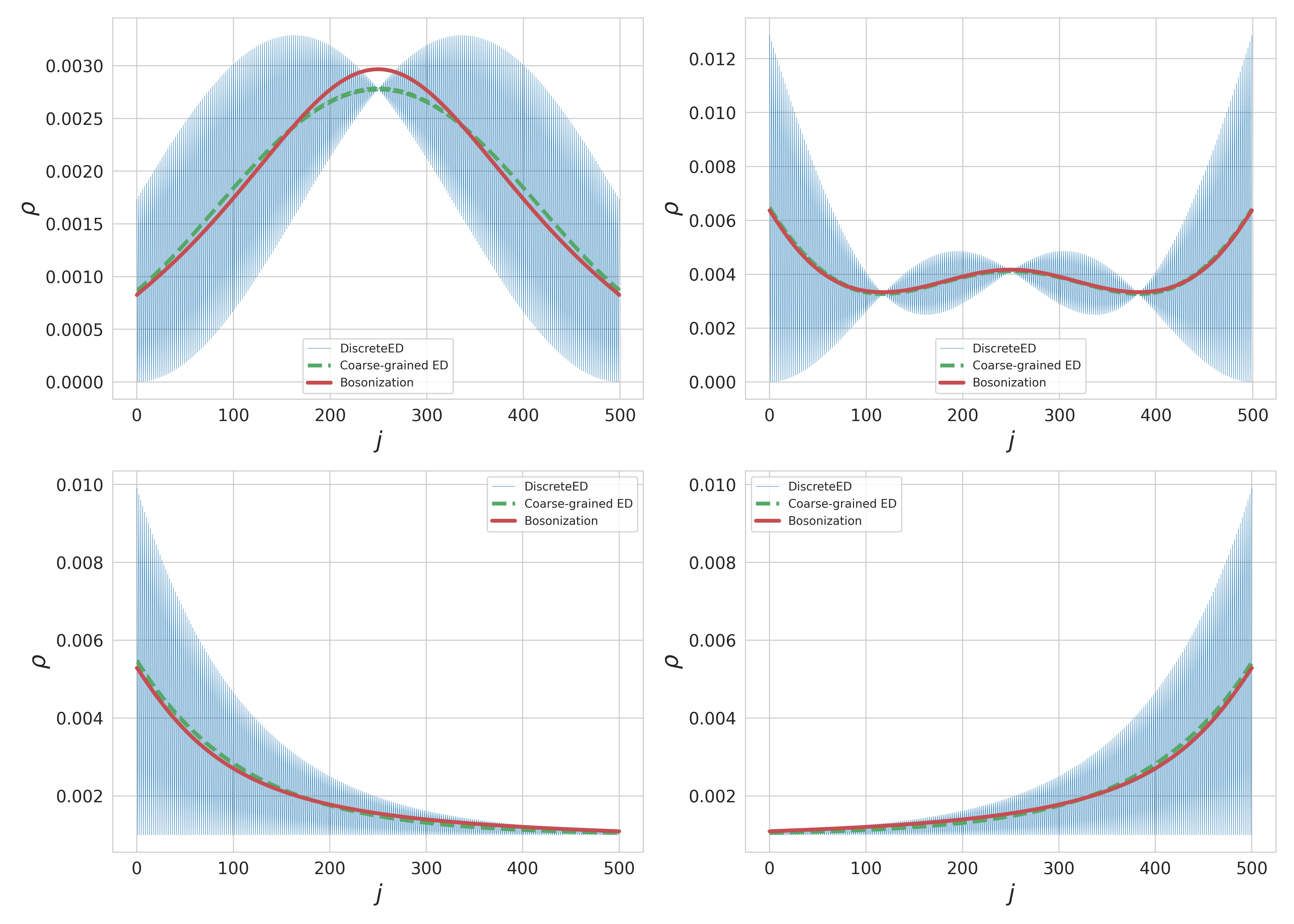
Figure 3: Additional plots comparing the solutions of the bosonization EL equations and the ED results. All the plots are done with $|\Delta|=7$ and $t=1$ Top-Left : First excited state of the trivial phase $N=500$, $\delta<0$, $n_{{\rm R}}=1$. Top-Right : Second excited state of the topological state $N=500$, $\delta>0$, $n_{{\rm R}}=2$. Bottom-Left : Odd number of sites $N=501$, $\delta>0$, $n_{{\rm R}}=1$. Bottom-Right : Odd number of sites $N=501$, $\delta<0$, $n_{{\rm R}}=1$.