Unsupervised Acoustic Scene Mapping Based on Acoustic Features and Dimensionality Reduction

Abstract

Classical methods for acoustic scene mapping require the estimation of time difference of arrival (TDOA) between microphones. Unfortunately, TDOA estimation is very sensitive to reverberation and additive noise. We introduce an unsupervised data-driven approach that exploits the natural structure of the data. Our method builds upon local conformal autoencoder (LOCA) – an offline deep learning scheme for learning standardized data coordinates from measurements. Our experimental setup includes a microphone array that measures the transmitted sound source at multiple locations across the acoustic enclosure. We demonstrate that LOCA learns a representation that is isometric to the spatial locations of the microphones. The performance of our method is evaluated using a series of realistic simulations and compared with other dimensionality-reduction schemes. We further assess the influence of reverberation on the results of LOCA and show that it demonstrates considerable robustness.

Index Terms—  acoustic scene mapping, relative transfer function (RTF), unsupervised learning, local conformal autoencoder (LOCA), dimensionality reduction

1 Introduction

From augmented reality to robot autonomy, in many audio applications, it is essential to map the environment and the shape of the room. Consequently, there has been a growing attention towards the task of simultaneous localization and mapping (SLAM). In SLAM, we consider a moving observer following an unknown path, and the task is then to reconstruct both the trajectory and the map of the environment. Due to the rapid improvement of computer vision technology, visual SLAM [1], based on optical sensors, has been the subject of extensive research. The same concept was later adopted by the audio processing community, as spatial information can also be extracted from the audio signals [2, 3].

In this work, we focus on the environment mapping problem using audio signals acquired by a microphone array, which is closely related to the acoustic SLAM problem. Traditionally, the environment map is specified in terms of landmarks, and reconstruction of the map is equivalent to localizing the landmarks [1]. Practically, acoustic SLAM methods necessitate the use of localization techniques, usually based on TDOA estimation between microphone pairs [2, 3]. The most widely used approach for TDOA estimation is the generalized cross-correlation (GCC-PHAT) algorithm [4]. Unfortunately, the performance of the GCC-PHAT algorithm severely degrades in highly reverberated environments [5], resulting in erroneous TDOA estimates and poor source localization, especially for large source-sensor distances. Consequently, some improvements to the GCC methods were proposed in [6, 7]. Nevertheless, simple TDOA-based mapping methods cannot yield a reliable reconstruction of the environment map.

Our novel approach utilizes recent progress from the manifold learning field, enabling us to deal with the problem of acoustic scene mapping in an entirely multi-path setting, thus circumventing the need to first extract the TDOA. Our framework requires a device-mounted microphone array that travels around the room in a scanner-like manner. The signals emitted from fixed sound sources are recorded at each point, and the RTFs are estimated. The estimated RTFs are high-dimensional feature vectors lying on manifolds. They can be naturally integrated with the LOCA dimensionality reduction scheme [8], enabling the inference of a latent space representation. The learned representation captures the latent variables that parameterize the data, i.e., it can recover the 2-D region of interest (RoI). One key advantage of LOCA over classic methods is that it can be used to predict the locations of measurements that were not seen during training. Moreover, the proposed method does not require the estimation of the TDOA and is relatively robust to reverberation.

2 Theoretical Background

2.1 The relative transfer function (RTF)

As mentioned above, we use RTFs [9] as the acoustic feature for our approach. RTFs are acoustic features independent of the source signal. Since they carry relevant spatial information, they can serve as “spatial fingerprints” that characterize the positions of each of the sources in a reverberant enclosure [10].

RTF - Definition and Estimation: For a pair of microphones, we consider time-domain acoustic recordings of the form

$$d_{i}(n)=\{a_{i}\ast s\}(n)+u_{i}(n),$$ (1)

with $s(n)$ being the source signal, $a_{i}(n)$, the room impulse responses relating the source and each of the microphones, $i=\{1,2\}$, and $u_{i}(n)$ noise signals, which are independent of the source. We define the acoustic transfer functions $A_{i}(k)$ as the Fourier transform of the RIRs $a_{i}(n)$. Following [9], the RTF is defined as $H(k)=\frac{A_{2}(k)}{A_{1}(k)}$. Assuming negligible noise and selecting $d_{1}(n)$ as the reference signal, the RTF can be estimated from:

$$\hat{H}(k)=\frac{\hat{S}_{d_{2}d_{1}}(k)}{\hat{S}_{d_{1}d_{1}}(k)}\approx H(k),$$ (2)

where $\hat{S}_{d_{1}d_{1}}(k)$ and $\hat{S}_{d_{2}d_{1}}(k)$ are the power spectral density (PSD) and the cross-PSD, respectively.

Representing RTFs on the Acoustic Manifold: Previous works have studied the nature of the RTFs. RTFs are high-dimensional representations in $\mathbb{C}^{D}$ that correspond to the vast amount of reflections from different surfaces characterizing the enclosure. Following the manifold hypothesis [11], we assume that the RTF vectors, drawn from a specific RoI in the enclosure, are not spread uniformly in the entire space of $\mathbb{C}^{D}$. Instead, they are confined to a compact manifold $\mathcal{M}$ of dimension $d$, which is much smaller relative to the ambient space dimension, i.e., $d\ll D$. This assumption is justified by the fact that perturbations of the RTF are only influenced by a small set of parameters related to the physical characteristics of the environment. These parameters include the enclosure dimensions, its shape, the surfaces’ materials, and the positions of the microphones and the source. Moreover, we focus on a static configuration, where the enclosure properties and the source position remain fixed. In such an acoustic environment, the only varying degree of freedom is the location of the microphone array.

With that being said, we assume that the RTFs can be intrinsically embedded in a low-dimensional manifold governed by the device’s position. The existence of such an acoustic manifold was discussed in detail in [12, 13, 10] and was shown to correspond with the position of the source. The assumed manifold is of reduced dimension and might have a complex nonlinear structure. In small neighborhoods, however, the manifold is locally linear, meaning that in the vicinity of each point, it is flat and coincides with the tangent plane to the manifold at that point. Hence, the Euclidean distance can faithfully measure affinities between points that reside close to each other on the manifold. For remote points, however, the Euclidean distance is meaningless. This property is utilized to our advantage by LOCA, which makes use of the relation between points in a local neighborhood.

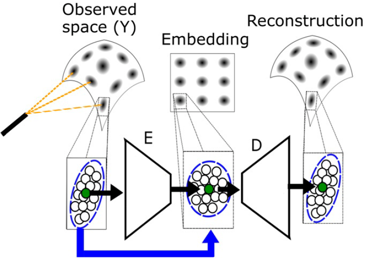
Fig. 1: An illustration of the LOCA framework. The observation space $(\mathcal{Y})$ is assumed to model a nonlinear deformation of the inaccessible manifold $(\mathcal{X})$. We attempt to invert the unknown measurement function, utilizing the bursts sampling strategy. LOCA consists of an encoder ($E$) parameterized by $\rho$ and a decoder ($D$) parameterized by $\gamma$. The autoencoder receives a set of points along with corresponding neighborhoods; each neighborhood is depicted as a dark oval point cloud (at the top of the figure). At the bottom, we zoom in onto a single anchor point $y_{i}$ (green) along with its corresponding neighborhood $Y_{i}$ (bounded by a blue ellipsoid). The encoder attempts to whiten each neighborhood in the embedding space while the decoder tries to reconstruct the input.

2.2 Local Conformal Autoencoder (LOCA)

Motivation: Our approach requires using a localized sampling strategy denoted burst sampling [14].

A burst is a collection comprising samples taken from a local neighborhood. Consequently, bursts can be used to provide information on the local variability in the neighborhood of each data point, allowing for the estimation of the Jacobian (up to an orthogonal transformation) of the unknown measurement function.

Assumptions and Derivation: First, for simplicity, we consider the case where the latent domain of our system of interest is a path-connected domain in the Euclidean space $\mathcal{X}\subset\mathbb{R}^{d}$. Observations of the system consist of samples captured by a measurement device and are given as a nonlinear smooth and bijective function $f:\mathcal{X}\rightarrow\mathcal{Y}$ where $\mathcal{Y}$ is the ambient, or measurement space. In our setting, the measurement space satisfies $\mathcal{Y}\subset\mathbb{R}^{D}$ where $d\ll D$.

Consider $N$ data points, denoted $\bm{x}_{1},\ldots,\bm{x}_{N}\in\mathbb{R}^{d}$ in the latent space. Assume that all these points lie on a path-connected, $d$-dimensional subdomain of $\mathcal{X}$. Importantly, we do not have direct access to the latent space $\mathcal{X}$. Samples in the latent space $\mathcal{X}$, which can be thought of as latent states, are pushed forward to the ambient space $\mathcal{Y}$ via the unknown deformation $f$. Let $\{\bm{y}_{i}\}_{i=1}^{N}$ (for $i=1,...,N$) where $\bm{y}_{i}=f(\bm{x}_{i})$, such that $\bm{y}_{1},\ldots,\bm{y}_{N}\in\mathbb{R}^{D}.$ We assume that the observed burst around $\bm{y}_{i}$ consists of perturbed versions of the latent state $\bm{x}_{i}$, pushed through the unknown deformation $f$. Formally, for fixed $1\leq i\leq N$, let $\bm{y}_{i}^{(1)},\ldots,\bm{y}_{i}^{(M)}$ be independent and identically distributed samples of the random variable $\bm{Y}_{i}=f(\bm{X}_{i})\in\mathbb{R}^{D}$, where $\bm{X}_{i}\sim\mathcal{N}(\bm{x}_{i},{\sigma}^{2}\bm{I}_{d})$ for $i=1,\ldots,N$ are independent random variables, and the number of samples taken from each burst is denoted by $M$.

The available data consists of $N$ sets of observed states, where each set, indexed by $1\leq i\leq N$, is $\{\bm{y}_{i}^{(j)}\}_{j=1}^{M}$. We assume that $\sigma$ is sufficiently small such that the differential of $f$ practically does not change within a ball of radius $\sigma$ around any point. Such sufficiently small $\sigma$ allows us to capture the local neighborhoods of the states at this measurement scale on the latent manifold.

Ideally, being able to find $f^{-1}:\mathcal{Y}\rightarrow\mathcal{X}$ would suffice to reconstruct the latent domain, but even if $f$ is invertible, it is generally not feasible to identify $f^{-1}$ without access to $\mathcal{X}$. We can, however, try to construct an embedding $\rho:\mathbb{R}^{D}\rightarrow\mathbb{R}^{d}$ that maps the observations $\{\bm{y}_{i}\}\in{\mathcal{Y}}$ so that the image of $\rho\circ f$ is isometric to $\mathcal{X}$ when $\sigma$ is known. In our Euclidean setting, it is equivalent to require that the distances in the latent space are preserved, i.e., samples should satisfy $\left\lVert\rho(\bm{y}_{i})-\rho(\bm{y}_{j})\right\rVert_{2}=\left\lVert\bm{x}_{i}-\bm{x}_{j}\right\rVert_{2}$ for any $i,j$.

Following the mathematical derivation in [8], the embedding $\rho$ that preserves the distances should satisfy the following condition

$$\frac{1}{{\sigma}^{2}}{\bm{C}(\rho(\bm{Y}_{i}))}=\bm{I},$$ (3)

where $\bm{Y}_{i}$ are the sample clouds (bursts), and $\bm{C}$ is the covariance matrix computed over the embedding of the samples from each burst. In other words, (3) requires that the covariance of samples from a local neighborhood in the embedding domain is whitened.

Implementation: As stated above, our task is to learn the embedding function $\rho$. We use an encoder neural network $(E)$ to learn the embedding function. Following (3), we define the loss term:

$$L_{\textrm{white}}(\rho)=\frac{1}{N}\sum_{i=1}^{N}\left\lVert\frac{1}{{\sigma}^{2}}{\bm{\hat{C}}(\rho(\bm{Y}_{i}))}-\bm{I}_{d}\right\rVert_{F}^{2},$$ (4)

where $\rho$ is the embedding function at the current iteration and $\bm{\hat{C}}(\rho(\bm{Y}_{i}))$ is the empirical covariance over a set of $M$ realizations $\{\rho(\bm{y}_{i}^{(j)})\}_{j=1}^{M}$. Next, we note that $f$ is an invertible function, and so is its inverse $f^{-1}$. Since our embedding $\rho$ tries to estimate $f^{-1}$ up to an orthogonal transformation, we enforce the invertibility of $\rho$ to reduce ambiguity in the solution. The invertibility of $\rho$ means that there exists an inverse mapping $\gamma:\mathbb{R}^{d}\rightarrow\mathcal{Y}$ such that $\bm{y}_{i}=\gamma(\rho(\bm{y}_{i}))$ for any $1\leq i\leq N$. By imposing an invertibility property on $\rho$, we effectively regularize the solution of $\rho$ away from noninvertible functions. Practically, we impose invertibility by using a decoder neural network $(D)$ parameterized by $\gamma$. This approach induces a new loss term based on the mean square error (MSE) between the input samples and their reconstructed counterparts:

$$L_{\textrm{recon}}(\rho,\gamma)=\frac{1}{N\cdot{M}}\sum_{i,m=1}^{N,M}\left\lVert\bm{y}_{i}^{(m)}-\gamma(\rho(\bm{y}_{i}^{(m)}))\right\rVert_{2}^{2}.$$ (5)

The LOCA framework is schematically depicted in Fig. 1.

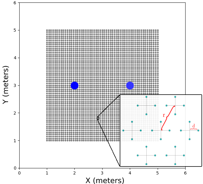
Fig. 2: Room sampling strategy - visualization of the room. Blue circles denote the location of the sound sources. The sampling grid along which the device travels is shown in grey. We zoom in to show the configuration of the burst microphone array: seven cross-like components consisting of vertical and horizontal microphone pairs.

3 Simulation

Experimental Setup: We construct a microphone array comprising seven cross-shaped sub-arrays in a circular constellation, each consisting of four omni-directional microphones, to implement the burst sampling strategy. The distance between the microphones in each arm of the cross is $2d$, and the radius w.r.t. the center of the constellation is $r$. For a relatively small radius, this circular array accurately simulates a Gaussian neighborhood sampled in the latent domain, as the burst sampling strategy requires.

Consider a room of dimensions $[6,6,2.4]$ m. Define a RoI within the room of size $4$x$4$ m, which is symmetrically positioned around the center of the room, $0.2$ m above the room’s floor. This setup alleviates strong reflections from the room facets. The microphone array is free to move on a grid with a spatial resolution of $56$ samples along each dimension, yielding a total of $N=3136$ bursts, with a spacing of $7.27$ cm between the centers of neighboring bursts. Additionally, two omni-directional sound sources are placed at $[x,y,z]=[2,3,1.7]$ m and $[x,y,z]=[4,3,1.7]$ m, lying $1.5$ m above the sampling-grid plane. The height of the sound sources above the sampling plane is vital due to simple geometric considerations. It allows phase accumulation between received signals in all directions relative to the sources. In addition, it became apparent by a series of experiments that using only a single emitting source may produce heavily deformed embeddings at the edges far from the source. For that reason, we used two sources in the simulations. A top-view visualization of the sampling constellation is shown in Figure 2. Note that the sound sources are not simultaneously active, thus allowing for the estimation of the individual RTFs.

Fig. 3: A visualization of the RTF input features corresponding to the vertical microphone pair components of the leftmost sampling grid-line, for $\textrm{RT}_{60}=360$ ms. A line in the grid consists of $56$ bursts, each containing $M=7$ RTFs, overall yielding $392$ RTFs. Each group of $7$ consecutive columns in the figure belongs to a different burst, appearing according to their order along the line. The data consists of an upper and a lower block, corresponding to the real and the imaginary parts of the RTFs, respectively.

Reverberated Data and Training: The reverberant acoustic data was generated using the GPU-accelerated RIR Simulator [15, 16]. The synthetic RIRs were convolved with $5$ second long white noise signals. We examined three reverberation times ($\textrm{RT}_{60}=160,360,610$ ms), set the sampling frequency to $f_{s}=16$ kHz and the speed of sound to $c=343$m/s. We also set the parameters for the microphone array to $r=2$ cm and $d=3$ cm. Using this configuration, at any given location and for each source, we can estimate the horizontal RTFs and the vertical RTFs, having a total of seven horizontal and seven vertical RTFs for a single burst. RTF estimation was applied according to (2), using $N_{FFT}=256$, with 50% overlapping Hamming windows. A single estimated RTF is a complex-valued feature of length $\frac{N_{FFT}}{2}+1=129$. For working with real-valued deep neural networks, we concatenated the real and imaginary parts to form a 258-dimension real-valued feature. Figure 3 visualizes the input features received from the vertical RTFs of the leftmost sampling grid-line in the room for the moderate $360$ ms reverberation time. It turns out (as discussed in Sec. 4) that picking a portion of the RTF bins is preferable. We obtain the best results when taking bins 5 to 99, corresponding to frequencies $312.5$–$6190$ Hz.

Our data tensor is constructed as follows: we take 95 bins from each complex RTF for each single sound source to construct a real-valued feature of length 190. Since we have both vertical and horizontal RTF components in our burst, we concatenate them to obtain a feature vector of length 380. Finally, having two speech sources, we repeat the process and concatenate both results. We eventually end up with a data tensor of shape $[N,M,D]=[3136,7,760]$. In terms of the LOCA terminology, we can write that $\mathcal{Y}\subset\mathbb{R}^{760}$, and we wish to reconstruct a 2-D latent embedding, $\mathcal{X}\subset\mathbb{R}^{2}$.

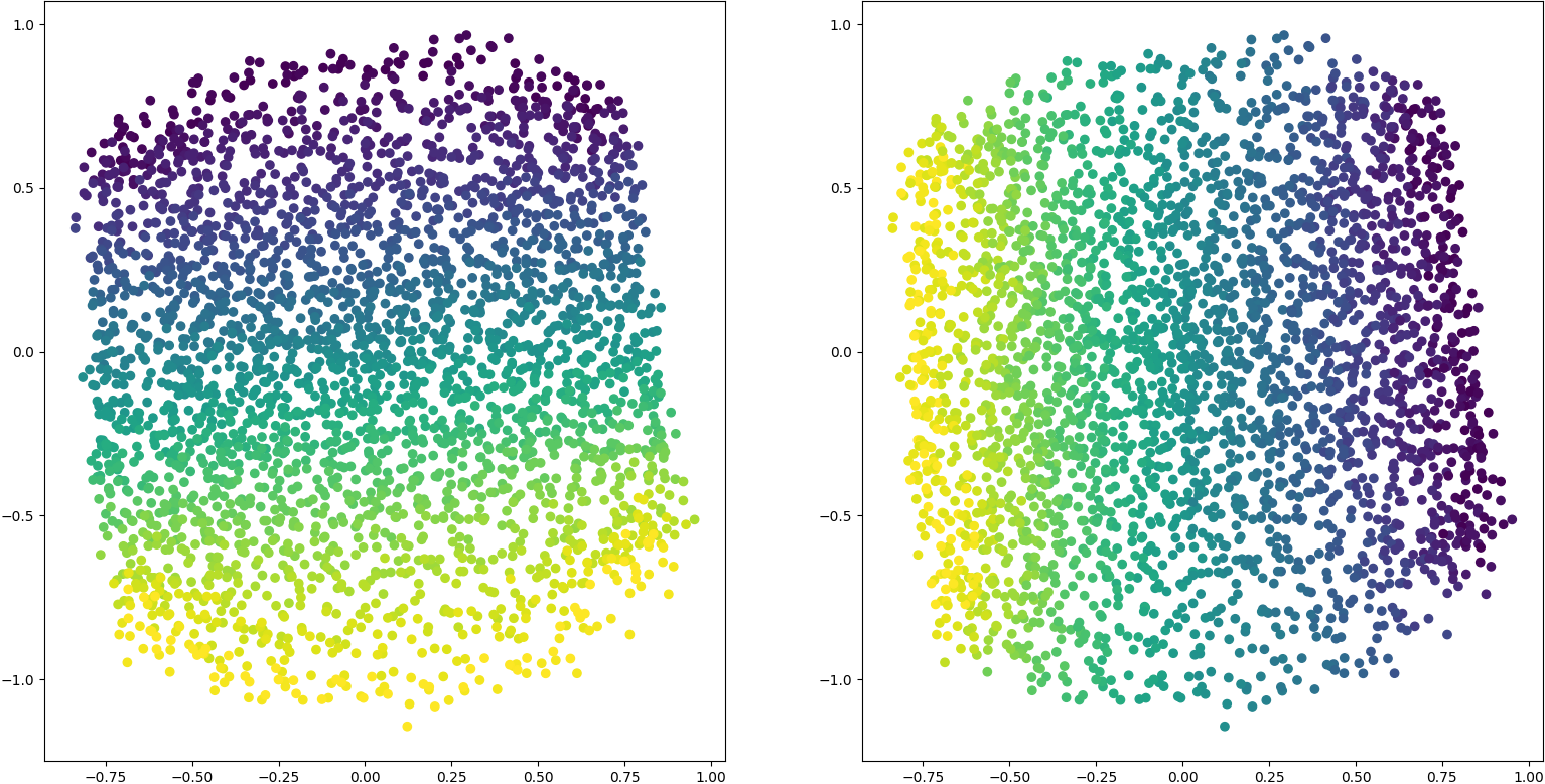
(a) $\textrm{RT}_{60}=360$ ms

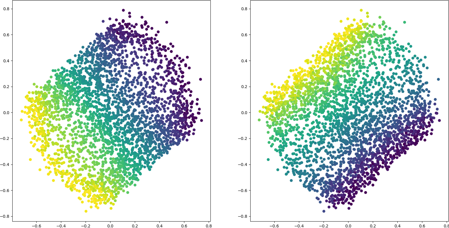
(b) $\textrm{RT}_{60}=610$ ms

Fig. 4: 2-D geometric reconstruction achieved by LOCA. Each reconstruction is displayed twice to show its correlation with the true coordinate axes of the original scene. The left and right panels correspond to the correlation with the X and Y axes, respectively.

Training and Parameters: We implemented both the encoder and decoder using simple feed-forward architectures. The encoder consists of an initial layer of dimension $D$ with no nonlinearity, followed by five layers of size $200$ with leaky-relu activations, ending with a latent representation layer of size $d$. Similarly, the decoder consists of the latent representation layer with no nonlinearity, followed by four layers of size $200$ with tanh activations, an additional linear layer of size $200$, and an output reconstruction layer of size $D$. We use a batch size of $2048$ samples and a learning rate of $1e^{-3}$. We use $90\%$ of the data during training, and the rest $10\%$ are used for validation and saving the best model weights. Finally, using the geometric measures of the microphone burst setup, we determine $\sigma$ value as $6e^{-4}$.

4 Simulation Study and Analysis

In Fig. 4, we visualize the embedding provided by LOCA. It is evident that LOCA demonstrates a high correlation between the main directions of the embedding and the true $x-y$ axes characterizing the square sampling grid. It is true that as the reverberation level increases, the embedding deforms. Overall, the model can still capture the directional correlation and reveal the square shape of the grid. We suspect that the reverberation-attributed degradation stems from the requirement of LOCA that $f$ is a smooth function. Inspecting Fig. 3, it is apparent that reverberation introduces artifacts into the RTF. In the presence of high reverberation, small perturbations in the location translate to relatively sharp changes in the RTF, meaning that $f$ is less smooth. Figure 5 depicts the distance between two RTFs from the same burst as a function of the frequency bin. RTFs taken from adjacent locations should vary minimally. However, we can clearly notice that the absolute difference in the highest frequency bins becomes larger and shows much higher variability, contrary to the smoothness requirement. Moreover, the low frequency bins show negligible differences since they hardly accumulate phase differences, rendering them useless for the localization task. For that reason, we take only a part of the frequency bins to achieve better results.

	$160$ ms	$360$ ms	$610$ ms
PCA	75.8	74.7	75.9
MMDS	73.3	79.5	82.8
DM	26.2	23.6	69.8
A-DM	18.4	25.4	33.8
LOCA	$\mathbf{13.1}$	$\mathbf{14.9}$	$\mathbf{18.7}$

Table 1: MAE (cm) comparison of the embeddings gained by each method.

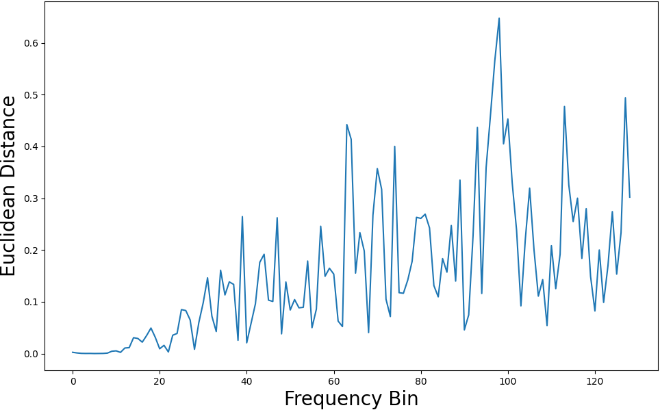
Fig. 5: The Euclidean distance vs. frequency bin between two adjacent RTFs ($\textrm{RT}_{60}=360$ ms) taken from the same burst.

Next, we would like to compare the results with other methods. Since we focus on unsupervised acoustic scene mapping, we compare LOCA to alternative dimensionality reduction methods. Specifically, we compare to: Principal-Component-Analysis (PCA), Metric-Multi-Dimensional-Scaling (MMDS) [17], diffusion maps (DM)[18], and anisotropic diffusion maps (A-DM) [14]. The above methods are commonly used in manifold learning and are justified by our assumption of the existence of the acoustic manifold. Hence they may serve as valid candidates for comparison. Note that we test these schemes over the same data used to train LOCA.

To quantify the performance, we calculate the mean absolute error (MAE) of the distance between the positions in the embedding space and their matching counterparts in the latent space. Note that we first calibrate the embedding using an orthogonal transformation and a shift before calculating the MAE. Additionally, in DM and A-DM, where we need to perform hyper-parameter tuning for $\sigma$, we first find the optimal $\sigma$ value by picking the embedding that leads to the minimal MAE, given a small set of four points of known location. In Table 1, we compare the performance of the competing methods, showing the influence of the reverberation time. It is apparent that LOCA leads to the best results in terms of MAE.

5 Conclusions

In this work, we harness recent advances in the field of DNN-based manifold learning to deal with the real-life problem of acoustic scene mapping in a multi-path setting. We demonstrate the applicability of the RTF as a proper and concise feature vector, which encapsulates the relevant spatial information for the task at hand. We apply an approach that utilizes the natural structure of the data and the local relations between samples, avoiding the severe performance degradation that is typical to classical localization approaches. Our simulation results confirm the robustness of the approach even in mild to high reverberation levels.

References

- [1] Hugh Durrant-Whyte and Tim Bailey, “Simultaneous localization and mapping: part i,” IEEE robotics & automation magazine, vol. 13, no. 2, pp. 99–110, 2006.
- [2] Jwu-Sheng Hu, Chen-Yu Chan, Cheng-Kang Wang, and Chieh-Chih Wang, “Simultaneous localization of mobile robot and multiple sound sources using microphone array,” in 2009 IEEE International Conference on Robotics and Automation, 2009, pp. 29–34.
- [3] Christine Evers and Patrick A. Naylor, “Acoustic SLAM,” IEEE/ACM Transactions on Audio, Speech, and Language Processing, vol. 26, no. 9, pp. 1484–1498, 2018.
- [4] C. Knapp and G. Carter, “The generalized correlation method for estimation of time delay,” IEEE Transactions on Acoustics, Speech, and Signal Processing, vol. 24, no. 4, pp. 320–327, Aug. 1976.
- [5] B. Champagne, S. Bedard, and A. Stephenne, “Performance of time-delay estimation in the presence of room reverberation,” IEEE Transactions on Speech and Audio Processing, vol. 4, no. 2, pp. 148–152, Mar. 1996.
- [6] M.S. Brandstein and H.F. Silverman, “A robust method for speech signal time-delay estimation in reverberant rooms,” in 1997 IEEE International Conference on Acoustics, Speech, and Signal Processing, 1997, vol. 1, pp. 375–378 vol.1.
- [7] Tsvi G. Dvorkind and Sharon Gannot, “Time difference of arrival estimation of speech source in a noisy and reverberant environment,” Signal Processing, vol. 85, no. 1, pp. 177–204, Jan. 2005.
- [8] Erez Peterfreund, Ofir Lindenbaum, Felix Dietrich, Tom Bertalan, Matan Gavish, Ioannis G. Kevrekidis, and Ronald R. Coifman, “Local conformal autoencoder for standardized data coordinates,” Proceedings of the National Academy of Sciences, vol. 117, no. 49, pp. 30918–30927, Nov. 2020.
- [9] S. Gannot, D. Burshtein, and E. Weinstein, “Signal enhancement using beamforming and nonstationarity with applications to speech,” IEEE Transactions on Signal Processing, vol. 49, no. 8, pp. 1614–1626, 2001.
- [10] Bracha Laufer-Goldshtein, Ronen Talmon, and Sharon Gannot, “Data-driven multi-microphone speaker localization on manifolds,” Foundations and Trends in Signal Processing, vol. 14, no. 1–2, pp. 1–161, 2020.
- [11] Joshua B. Tenenbaum, Vin de Silva, and John C. Langford, “A global geometric framework for nonlinear dimensionality reduction,” Science, vol. 290, no. 5500, pp. 2319–2323, Dec. 2000.
- [12] Bracha Laufer-Goldshtein, Ronen Talmon, and Sharon Gannot, “Semi-supervised sound source localization based on manifold regularization,” IEEE/ACM Transactions on Audio, Speech, and Language Processing, vol. 24, no. 8, pp. 1393–1407, Aug. 2016.
- [13] Bracha Laufer-Goldshtein, Ronen Talmon, and Sharon Gannot, “A study on manifolds of acoustic responses,” in Latent Variable Analysis and Signal Separation, pp. 203–210. Springer International Publishing, 2015.
- [14] Amit Singer and Ronald R. Coifman, “Non-linear independent component analysis with diffusion maps,” Applied and Computational Harmonic Analysis, vol. 25, no. 2, pp. 226–239, Sept. 2008.
- [15] David Diaz-Guerra, Antonio Miguel, and Jose R. Beltran, “gpuRIR: A python library for room impulse response simulation with GPU acceleration,” Multimedia Tools and Applications, vol. 80, no. 4, pp. 5653–5671, Oct. 2020.
- [16] Jont B Allen and David A Berkley, “Image method for efficiently simulating small-room acoustics,” The Journal of the Acoustical Society of America, vol. 65, no. 4, pp. 943–950, 1979.
- [17] Hervé Abdi, “Metric multidimensional scaling (mds): analyzing distance matrices,” Encyclopedia of measurement and statistics, pp. 1–13, 2007.
- [18] Ronald R Coifman and Stéphane Lafon, “Diffusion maps,” Applied and computational harmonic analysis, vol. 21, no. 1, pp. 5–30, 2006.