Robust Domain Adaptive Object Detection with
Unified Multi-Granularity Alignment

Abstract

Domain adaptive detection aims to improve the generalization of detectors on target domain. To reduce discrepancy in feature distributions between two domains, recent approaches achieve domain adaption through feature alignment in different granularities via adversarial learning. However, they neglect the relationship between multiple granularities and different features in alignment, degrading detection. Addressing this, we introduce a unified multi-granularity alignment (MGA)-based detection framework for domain-invariant feature learning. The key is to encode the dependencies across different granularities including pixel-, instance-, and category-levels simultaneously to align two domains. Specifically, based on pixel-level features, we first develop an omni-scale gated fusion (OSGF) module to aggregate discriminative representations of instances with scale-aware convolutions, leading to robust multi-scale detection. Besides, we introduce multi-granularity discriminators to identify where, either source or target domains, different granularities of samples come from. Note that, MGA not only leverages instance discriminability in different categories but also exploits category consistency between two domains for detection. Furthermore, we present an adaptive exponential moving average (AEMA) strategy that explores model assessments for model update to improve pseudo labels and alleviate local misalignment problem, boosting detection robustness. Extensive experiments on multiple domain adaption scenarios validate the superiority of MGA over other approaches on FCOS and Faster R-CNN detectors. Code will be released at https://github.com/tiankongzhang/MGA.

1 Introduction

Object detection has been one of the most fundamental problems in computer vision with a long list of applications such as visual surveillance, self-driving, robotics, etc. Owing to the powerful representation by deep learning (e.g., [2, 3, 4]), object detection has witnessed considerable advancement in recent years with numerous excellent frameworks (e.g., [5, 6, 7, 8, 9, 10, 11, 12]). These modern detectors are usually trained and evaluated on a large-scale annotated dataset (e.g., [13]). Despite the great achievement, they may suffer from poor generalization when applied to images from a new target domain. To remedy this, a simple and straightforward solution is to build a benchmark for the new target domain and re-train the detector. Nevertheless, benchmark creation is both time-consuming and costly. In addition, the new target domain could arbitrary and it is almost impossible to develop benchmarks for all new target domains.

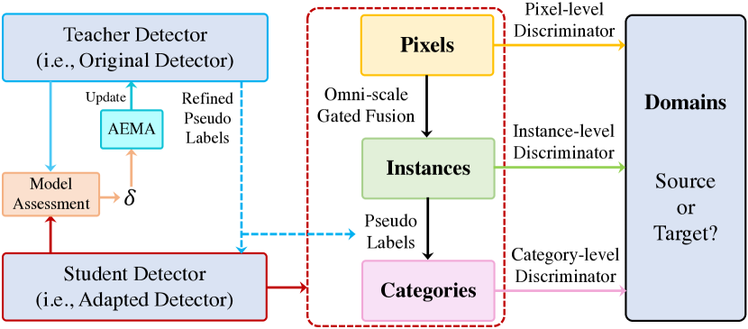
Figure 1: Illustration of the proposed Multi-Granularity Alignment (MGA) framework for domain adaptive object detection. Specifically, MGA encodes the dependencies across multiple granularities simultaneously, including pixel-, instance-, and category-levels. In addition, a dynamic update mechanism guided by update factor $\delta$ (as detailed later) through model assessment during training is used to improve the quality of pseudo labels and meanwhile mitigate the local misalignment problem, further enhancing the detection robustness. Best viewed in color and by zooming in for all figures throughout this paper.

In order to deal with the above issues, researchers have explored the unsupervised domain adaption (UDA) detection, with the goal of transferring knowledge learned from an annotated source domain to an unlabeled target domain. One popular trend is to leverage adversarial learning [14] to narrow the discrepancy between domains. Specifically, a domain discriminator is introduced to distinguish which domain, the source or the target, the image comes from. Then, the detector learns the domain-invariant feature representation by confusing the discriminator [15]. Despite achieving promising results, previous domain adaption approaches may suffer from target scale variations in cluttered regions due to the fixed kernel design in ConvNets [2, 3], which results in difficulty in learning discriminative representations for objects of different scales and thus degrades detection performance. For example, the features of small targets may contain too much background noise because of too large receptive field in the convolutional layer. Meanwhile, the features of large objects may lack global structural information owing to too small receptive field. In addition, the intrinsic relation of feature distributions between two domains are neglected.

To address the aforementioned problems, various feature alignment strategies have been introduced in the adversarial learning manner [14, 16] for better target domain adaption. These alignment approaches can be summarized into three categories based on different granularity perspectives, consisting of pixel-, instance-, and category-level. Pixel-level alignment [17, 18, 19] aims at aligning lower-level pixel feature distribution of objects and background regions. Nevertheless, there may exist a large gap between the pixel-level features for objects of different scales within the same category, resulting in limited detection performance. Different from pixel-level alignment, instance-level alignment [20, 21, 22, 23, 24] first pools the feature maps of detection proposals and then leverages the pooled proposal features for the domain discriminator training. Despite avoiding the gap in pixel-level alignment, this strategy suffers from feature distortion for objects of different scales and aspect ratios caused by the pooling operation, which may lead to inaccurate feature representation and degenerated results. In addition to the aforementioned two types of alignments, recent approaches have attempted to utilize category-level alignment [25, 26, 27, 28, 29, 30] for UDA detection. In specific, taking into consideration the intrinsic relation of feature distributions in two domains, the category-level alignment leverages the categorical discriminability to handle hard aligned instances. However, this alignment mechanism focuses only on the global consistency of feature distribution between two domains while ignores other local consistency constrains.

Contribution. Although each type of alignment strategy brings in improvement, they are limited in several aspects as discussed above. In order to address these issues and make full use of the advantages of these three alignments, we propose a novel unified Multi-Granularity Alignment (MGA) framework for UDA detection, as illustrated in Figure 1.

Instead of performing simple combination of different alignment methods, MGA simultaneously encodes the dependencies across different granularities, consisting of pixel-, instance-, and category-levels, for domain alignment. More specifically, we first introduce an omni-scale gated fusion (OSGF) module in MGA. The OSGF module is able to adapt to instances of different scales by automatically choosing the most plausible convolutions from the low- and high-resolution streams for feature extraction. Concretely, we first predict coarse detections based on pixel-level backbone feature maps. Then, using these coarse detections as guidance, we design a set of parallel convolutions in OSGF and adopt a gate mechanism to aggregate the discriminative features of instances (i.e., the coarse detections) with similar scales and aspect ratios. By doing so, the following detection head can more accurately predict multi-scale objects.

Besides the OSGF module, we present a new category-level discriminator. Different from previous approaches, our category-level discriminator takes into account not only the instance discriminability in different classes but also the category consistency between two domains, leading to better detection. In order to supervise the category-level discriminator, pseudo labels are assigned to important instances with high confidence based on object detection results.

Considering that the quality of pseudo labels is crucial for learning a good category-level discriminator, we propose a simple yet effective adaptive exponential moving average (AEMA) strategy to train the teacher detector (i.e., the original detector). As shown in Figure 1, during the training phase, we assess both the teacher detector and the student detector (i.e., the final adaptive detector) on the source domain. Based on their model assessments, a dynamic update factor $\delta$ (as described later) is learned and utilized as a guidance to adjust the coefficient parameter in exponential moving average (EMA) update in an adaptive manner. The resulted AEMA helps better train the teacher detector to produce high-quality pseudo labels and meanwhile alleviate the local misalignment caused by low-quality pseudo labels, significantly enhancing the detection robustness. We will elaborate on the details of our AEMA later.

By developing the multi-granularity discriminators, our MGA exploits and integrates rich complementary information from different levels, and hence achieves better UDA detection. Besides, the proposed AEMA further enhances the robustness with high-quality pseudo labels.

To validate the effectiveness of our approach, we carry out extensive experiments on multiple domain-shift scenarios using various benchmarks including Cityscapes [31], FoggyCityscapes [32], Sim10k [33], KITTI [34], PASCAL VOC [35], Clipart [36] and Watercolor [36]. We evaluate the proposed method on the top of two popular detection frameworks, the anchor-free FCOS [8] and the anchor-based Faster R-CNN [7], with VGG-16 [4] and ResNet-101 [2] backbones. Experiment results demonstrate that our MGA together with the dynamic model update significantly improve the baseline detectors with superior results over other state-of-the-arts.

To sum up, we make the following key contributions:

• We propose a novel unified multi-granularity alignment (MGA) framework that encodes dependencies across different pixel-, instance-, and category-levels for UDA detection. Notably, our MGA framework is general and applicable to different object detectors.

• We present an omni-scale gate fusion (OSGF) module to extract discriminative feature representation for instances with different scales and aspect ratios.

• we propose a new category-level discriminator by exploiting both the instance discriminability in different classes and the category consistency between two domains, leading to better detection.

• We introduce a simple yet effective dynamic adaptive exponential moving average (AEMA) strategy to improve the quality of pseudo labels and meanwhile mitigate the local misalignment issue in UDA detection, which significantly boosts the robustness of detector.

• On extensive experiments on multiple domain adaption scenarios, the proposed approach outperforms other state-of-the-art UDA detectors on the top of two detection frameworks, evidencing its effectiveness and generality.

This paper builds upon our preliminary conference version [1] and significantly extends it in different aspects. (1) We propose an effective assessment-based AEMA for model update of the teacher detector. This way, we are able to obtain pseudo labels with better quality, which largely boosts the detection robustness. Meanwhile, it is beneficial in alleviating the local misalignment issue caused by low-quality pseudo labels, further improving the performance. (2) We modify the structure of the OSGF module by sharing the convolutional layer (as described later). Note that, this modification is not trivial. It not only brings in improvement on the detection results but also decreases the number of parameters. (3) We incorporate more experiments and comparisons with in-depth analysis and ablation studies to further show the effectiveness of our approach. (4) We supplement thorough visual analysis of our detector, which allows the readers to better understand our method.

The rest of this paper is organized as follows. Section 2 discusses approaches related to this paper. Our approach is elaborated in Section 3. In Section 4, we demonstrate the experimental results, including comparisons with state-of-the-arts, ablation studies and visual analysis, followed by conclusion in Section 5.

2 Related Work

In this section, we review approaches relevant to this paper from four aspects, including object detection, UDA detection, alignment strategy for UDA detection and exponential moving average.

2.1 Object Detection

Object detection is a fundamental topic in computer vision and has been extensively studied for decades. In general, existing modern detectors can be categorized into either anchor-based or anchor-free. Anchor-based detectors usually contain a set of anchor boxes with different scales and aspect ratios, which are applied to generate object proposals for further processing (in two-stage frameworks) or final detections (in one-stage frameworks). One of the most popular anchor-based detectors is Faster R-CNN [7]. It introduces a novel region proposal network (RPN) to produce object proposals based on anchors and then applies another network to further process the proposals for detection. The approaches of SSD [10] and YOLOv2 [37] present one-stage anchor-based detectors that strikes a good balance between accuracy and speed. Later, more excellent anchor-based detectors [38, 39, 12, 40, 41, 42] are proposed for improvements. Different from anchor-based approaches, anchor-free detectors remove the manual design of anchor boxes and directly predict the class and coordinates of objects. YOLO [11] directly predicts the object class and position from grid cells. CornerNet [9] proposes to predict the object bounding boxes as keypoint detection. The work of CenterNet [43] improves CornetNet by considering an extra center point. FCOS [8] introduces the fully convolutional networks to predict object box of each pixel in feature maps. Recently, DETR [44] applies Transformer [45] to develop an anchor-free detector  and exhibits impressive performance.

In this paper, we utilize the proposed MGA upon the popular anchor-based Faster R-CNN [7] and anchor-free FCOS [8] to verify its effectiveness. But please note that, our MGA is general and flexible and can be used in more frameworks for UDA detection.

2.2 Unsupervised Domain Adaption (UDA) Detection

The task of unsupervised domain adaption (UDA) detection focuses on improving the generality of object detectors learned from labeled source images on unlabeled target images. Because of its great practicability, UDA object detection has attracted extensive attention in recent years. One popular framework is to leverage adversarial learning to achieve UDA detection [46, 47]. These approaches introduce a discriminator to identify which domain the features of pixels, regions or images come from. Then, the goal is to confuse the discriminator to learn domain-invariant features for detection. In addition, many other researchers propose to apply graph methods for UDA detection [48, 49, 50, 51]. These graph-based approaches propose to construct a graph based on regions or instances in an image and leverages the intra-class and inter-class relation of intra-domain and inter-domain for detection. Self-training strategy has also been explored in UDA detection [52, 53, 54, 55]. The main idea of these methods is to generate high-quality or class-balanced pseudo-labels, which can be utilized to train the detection model on the unlabeled target domain. The approaches of [56, 19, 57] leverage the idea of style transfer for UDA detection. In specific, these methods reduce the discrepancy of data distribution between two domains by translating the images of source domain to target style, which improves the generalization ability of the detector. Besides the aforementioned methods, recent approaches propose to apply mean-teacher for UDA detection [58, 59, 60]. These models adopt a teacher-student training framework to maintain the consistency of the teacher and student detector networks for boosting the generality of detection. Different from the above approaches, in this paper we tackle the UDA detection problem from a different perspective by unifying alignments of multiple granularities.

2.3 Alignment for UDA Detection

Alignment of feature distribution between source and target domains has demonstrated effectiveness for UDA detection. Accordingly to the features involved, recent alignment-based approaches can be categorized into three types including pixel-, instance-, and category-level alignments.

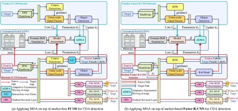
Figure 2: Framework of our MGA on the top of popular anchor-free FCOS [8] (see left image (a)) and anchor-based Faster R-CNN [61] (see right image (b)) for UDA detection with assessment-based AEMA. Note that for Faster R-CNN, the region proposal network (RPN) and the RoI head are used for coarse detection and final detection, respectively. $F$ in (a), $F_{1}$ and $F_{2}$ in (b) represent the features from the feature pyramid network in FCOS and backbone in Faster R-CNN.

Pixel-level Alignment. Pixel-level alignment focuses on aligning the pixel feature distributions of objects and background regions between two domains for UDA detection. The work of [18] takes into account every pixel for domain adaption and introduces a center-aware pixel-level alignment by paying more attention to foreground pixels for UDA detection. The approach of [17] designs the multi-domain-invariant representation learning to encourage unbiased semantic representation through adversarial learning. The method of [19] introduces an intermediate domain for progressive adaption and utilize adversarial learning for pixel-level feature alignment.

Instance-level Alignment. Instance-level alignment usually leverages features of regions or instances to train a domain discriminator. The approach of [20] explores the relation of different instances using mean-teacher based on Faster R-CNN [7] for UDA detection. The work of [21] introduces a hierarchical framework to align both instance and domain features for detection. The method of [22] proposes to adapt Faster R-CNN on target domain images by aligning features on instance- and image-levels, exhibiting promising performance. The approach of [23] introduces attention mechanisms for better alignment in UDA detection. Instead of using all instances or regions for alignment, the work of [24] proposes to mine the discriminative ones and focuses on aligning them across two different domains for adaption detection.

Category-level Alignment. Category-level alignment considers the intrinsic relation of feature distributions in source and target domains and exploits the categorical discriminability for alignment. The approaches of [25, 26, 27, 62] learn a category-specific discriminator for each category and focus on classification between two domains using pseudo labels. Despite effectiveness, it is difficult for these approaches to learn discriminative category-wise representation among multiple discriminators. The method of [28] retains one discriminator to distinguish different categories within one domain, whereas it neglects the consistency of feature subspaces in the same category across two domains. Besides, the work of [29] develops a categorical regularization method that focuses on important regions and instances to reduce the domain discrepancy. The method of [30] seeks for category-level domain alignment by enhancing intra-class compactness and inter-class separability.

Our Alignment. Despite sharing similar spirit in applying alignment for UDA object detection, our approach (i.e., Multi-Granularity Alignment (MGA)) is significantly different from others. Specifically, MGA is a unified framework that effectively encodes the dependencies across different granularities, including pixel-, instance-, and category-levels, for domain adaption detection, while other methods do not consider this important dependency relation in alignment. In addition, we specially design the omni-scale gated fusion (OSGF) module and present a new category-level discriminator in MGA to improve the discriminative ability, as detailed later.

2.4 Exponential Moving Average

Exponential moving average (EMA) is a simple but effective strategy for updating the model parameters and commonly utilized in distillation technology [63, 64, 65] and mean-teacher [66, 67]. In these approaches, the EMA process is usually controlled by a constant weight coefficient to update the teacher network. Despite effectiveness, this mechanism may hurt the performance of UDA detection due to the low-quality pseudo labels generated by the teacher detector. Therefore, unlike previous studies, we design an adaptive EMA (AEMA) by exploring the assessments of the teacher and student detector networks during training. AEMA is able to adjust the weight coefficient of EMA in an adaptive manner, leading to higher-quality pseudo labels for improvements.

3 Multi-Granularity Alignment (MGA)

3.1 Overview

In this paper, we propose a novel unified multi-granularity alignment (MGA) framework for domain adaption detection. The overall architecture is illustrated in Figure 2.

As displayed in Figure 2, given images from the source domain $s$ and the target domain $t$, we first extract the base pixel-level feature representation from the backbone. Then, these features are merged in the omni-scale gated fusion (OSGF) module to produce discriminative representations of multi-scale instances. Based on the fused feature representations, more accurate candidate objects can be predicted by the object detection head. Meanwhile, we introduce the multi-granularity discriminators to distinguish the feature distributions between two domains from different perspectives, including pixel-level, instance-level and category-level. Moreover, in order to improve the quality of pseudo labels and mitigate the misalignment issue caused by noisy pseudo labels during training, we propose a simple but effective assessment-based adaptive EMA (AEMA) strategy to refine the pseudo labels, further enhancing the robustness of our MGA for domain adaption detection.

It is worth noting that, our MGA is a general framework and can be easily applied in various detectors (e.g., anchor-free FCOS [8] and anchor-based Faster R-CNN [7]) with different backbones (e.g., VGG-16 [4] and ResNet-101 [2]). Without loss of generality, we first apply the proposed MGA in FCOS [8] for UDA object detection as in Figure 2 (a), and then explain how it can be used in Faster R-CNN [7] as in Figure 2 (b). For FCOS [8], we extract feature maps from the last three stages of the backbone and combine them into multi-level feature maps $F^{k}$, where $k\in\{3,4,5,6,7\}$, using FPN representation [68].

3.2 Omni-Scale Gated Object Detection

In most previous studies on domain adaption detection, the main goal is to designate discriminators at a specific level and some attentive regions. Nevertheless, the use of point representation at pixel-level in anchor-free models [18, 69] may cause difficulties in learning robust and discriminative feature in cluttered background, while the pooling operation (e.g., RoIAlign [39]) in anchor-based models [15, 70] may distort the features of the instances with different scales and aspect ratios.

In order to handle this problem, we introduce an omni-scale gated fusion (OSGF) module for object detection, which enables the adaption of the feature learning to object with various scales and aspect ratios. Specifically in OSGF, with the scale guidance from coarse detections, we can choose the most plausible convolutions with different kernels to extract compact features of instances in terms of object scales, which can significantly boost the discriminative capacity of the features. Our OSGF module is designed for general purpose and thus can be easily applied in different detectors.

3.2.1 Scale Guidance by Coarse Detection

In order to select the most plausible convolutions for feature extraction, it is necessary to obtain the scale information of the objects. To this end, we introduce a coarse detection step to provide the scale guidance. In specific, followed by the multi-level feature maps $F^{k}$ ($k\in\{3,4,5,6,7\}$ denotes the level index) from the backbone (see Figure 2 (a)), we can predict the candidate object boxes $\tilde{b}^{k}$ through a series of convolutional layers. Drawing inspiration from [71], we utilize the cross-entropy Intersection over Union (IoU) loss [72] to regress the bounding boxes of objects in foreground pixels as follows,

$$\mathcal{L}_{\text{gui}}=-\sum_{k}\sum_{(i,j)}\ln(\text{IoU}(\tilde{b}^{k}_{i,j},b^{k}_{i,j})),$$ (1)

where $\text{IoU}(\cdot,\cdot)$ represents the function to calculate the IoU score between predicted box $\tilde{b}^{k}$ and ground-truth box $b^{k}$. For each pixel $(i,j)$ in the feature map, the corresponding box $b^{k}_{i,j}$ can be defined as a $4$-dimensional vector as follows,

$$b^{k}_{i,j}=(x_{t_{i,j}},x_{b_{i,j}},x_{l_{i,j}},x_{r_{i,j}})$$ (2)

where $x_{t_{i,j}}$, $x_{b_{i,j}}$, $x_{l_{i,j}}$, and $x_{r_{i,j}}$ respectively represent the distances between current location and the top, bottom, left and right bounds of ground-truth box. Therefore, the normalized object scale (i.e., width $w^{k}$ and height $h^{k}$) at each level can be computed as follows,

$$\left\{\begin{aligned} &w^{k}_{i,j}=(\tilde{x}_{r_{i,j}}+\tilde{x}_{l_{i,j}})/\text{stride}^{k},\\ &h^{k}_{i,j}=(\tilde{x}_{b_{i,j}}+\tilde{x}_{t_{i,j}})/\text{stride}^{k},\\ \end{aligned}\right.$$ (3)

where $\text{stride}^{k}$ denotes how many steps we move in each round of convolution operation. As in FCOS [8], the feature maps at each level are utilized to individually detect the objects of different scales in the range $\{[-1,64]$, $[64,128]$, $[128,256]$, $[256,512]\}$, $[512,+\infty]\}$. Therefore, the majority of object scales is less than $8$, i.e., $w^{k}\leq 8,h^{k}\leq 8$. For notation simplicity, we omit the superscript $k$ and write $F$ for $F^{k}$ and $\tilde{b}$ for $\tilde{b}^{k}$ in the following sections.

3.2.2 Omni-scale Gated Fusion (OSGF)

With the scale guidance as in Section 3.2.1, we present an omni-scale gated fusion module (OSGF), which is composed of both low-resolution and high-resolution feature streams, to adapt to objects of various scales and aspect ratios. Specifically, as illustrated in Figure 3, the low-resolution stream consists of three parallel convolutional layers with different kernels $\omega\in\{3\times 3,3\times 5,5\times 3\}$, which is applied for feature extraction of relatively small objects ($w^{k}\leq 5,h^{k}\leq 5$). Meanwhile, in the high-resolution feature stream, we use another set of parallel convolutional layers with kernels $\omega$ to handle large objects ($w^{k}>5,h^{k}>5$). The different from the low-resolution feature branch is that, we utilize an extra upsampling operation after each convolutional layer in the high-resolution stream to upscale the feature maps. It is worth noticing that, the structure of OSGF in this paper is different from that in the conference publication [1]. In specific, the major modifications in this paper include: (i) removal of the $3\times 3$ convolutional layer before the two streams, (ii) incorporation of simpler averaging pooling and $1\times 1$ convolutional layers in the low-resolution stream, (iii) replacement of the $3\times 3$ convolutional layers with shared averaging pooling and $1\times 1$ convolutional layers, and (iv) change of the $1\times 1$ convolutional layer to $3\times 3$ convolutional layer in the residual connection. By doing so, the overall number of parameters are significantly reduced because of less convolutional layers used. In addition, we observe that the detection performance has been improved by designing the shared convolutional layer and increasing the kernel size in the convolutional layer of residual connection, as evidenced by our experiments.

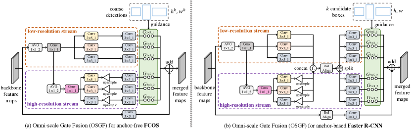
Figure 3: Illustration of the proposed omni-scale gated fusion (OSGF) module for anchor-free FCOS [8] (see left image (a)) and anchor-based Faster R-CNN [61] (see right image (b)). The parameters of the modules with the same color are shared.

After the two branches of low- and high-resolution features, we introduce a gate mask $G$ to weight each convolutional layer based on the predicted coarse boxes $\tilde{b}$ as follows,

$$G_{\omega}=\frac{\exp(\tau(o_{\omega}-\hat{o})/(\hat{o}+\epsilon))}{\sum_{\omega}\exp(\tau(o_{\omega}-\hat{o})/(\hat{o}+\epsilon))},$$ (4)

where $\tau$ represents the temperature factor, $o_{\omega}=\text{IoU}(\tilde{b},\omega)$ denotes the overlap between the predicted box and the convolution kernel $\omega$, and $\hat{o}$ is the maximal overlap among them. Finally, we merge the pixel-level features to exploit the scale-wise representation of instances as follows,

$$M=\sum_{\omega}F_{\omega}\odot G_{\omega}+F_{3\times 3},$$ (5)

where $\odot$ denotes the element-wise product, and $F_{\omega}$ denotes the feature maps after the convolutional layer with kernel $\omega$.

3.2.3 Object Detection

After obtaining the merged feature maps $M$ from the OSGF module, we can predict the categories and bounding boxes of objects. In FCOS [8], the object detection heads contain three branches for classification, centerness and regression, respectively. The classification and centerness branches are optimized by the focal loss [73] $\mathcal{L}_{\text{cls}}$ and cross-entropy loss [8] $\mathcal{L}_{\text{ctr}}$, respectively. The regression branch is optimized by the IoU loss [72] $\mathcal{L}_{\text{reg}}$. Thus, the final loss function $\mathcal{L}_{\text{det}}$ for the object detection is defined as

$$\mathcal{L}_{\text{det}}=\mathcal{L}_{\text{cls}}+\mathcal{L}_{\text{ctr}}+\mathcal{L}_{\text{reg}}.$$ (6)

Please refer to [8] for more details regarding the loss functions. It is worthy to notice that, in the UDA detection, we implement two detectors, including a teacher detector and a student detector (see Figure 2 (a)). These two detectors share the same architecture but independent parameters. We denote the loss functions for the teacher and the student detectors as $\mathcal{L}_{\text{det}}^{\mathcal{T}}$ and $\mathcal{L}_{\text{det}}^{\mathcal{S}}$, respectively.

3.3 Multi-Granularity Discriminators

As discussed earlier, we propose the multi-granularity discriminators to distinguish whether the sample belongs to the source domain or the target domain from various perspectives, consisting of pixels, instances and categories. The discrepancy between two domains is reduced using Gradient Reversal Layer (GRL) [14] that transfers reverse gradient when optimizing the object detection network. The discriminator contains four stacked convolution-groupnorm-relu layers and an extra $3\times 3$ convolutional layer. Below we will elaborate on our multi-granularity discriminators.

3.3.1 Pixel- and Instance-level Discriminators

The pixel- and instance-level discriminators are leveraged to respectively perform pixel-level and instance-level alignments of feature maps between two domains. As demonstrated in Figure 2 (a), given the input multi-level features $F$ and the merged feature $M$, the pixel-level and instance-level discriminators $D^{\text{pix}}$ and $D^{\text{ins}}$ are learned through the loss functions $\mathcal{L}_{\text{pix}}$ and $\mathcal{L}_{\text{ins}}$. Similar to previous work [18], we adopt the same loss function. Then, $\mathcal{L}_{\text{pix}}$ and $\mathcal{L}_{\text{ins}}$ are defined as follows

$$\begin{split}\mathcal{L}_{\text{pix}}=-\sum_{(i,j)}&y^{\text{pix}}_{i,j}\log D^{\text{pix}}(F^{s}(i,j))\\ &+(1-y^{\text{pix}}_{i,j})\log(1-D^{\text{pix}}(F^{t}(i,j))),\end{split}$$ (7)

$$\begin{split}\mathcal{L}_{\text{ins}}=-\sum_{(i,j)}&y^{\text{ins}}_{i,j}\log D^{\text{ins}}(M^{s}(i,j))\\ &+(1-y^{\text{ins}}_{i,j})\log(1-D^{\text{ins}}(M^{t}(i,j))),\end{split}$$ (8)

where $F(i,j)$ is the feature at pixel $(i,j)$ in $F$, and $M(i,j)$ the feature at instance $(i,j)$ in $M$. We have the domain label $y^{\text{pix}}_{i,j}=1$ if pixel at $(i,j)$ in $F$ is from source domain and $0$ otherwise. Likewise, $y^{\text{ins}}_{i,j}=1$ if the instance at $(i,j)$ in $M$ belongs to source domain and $0$ otherwise.

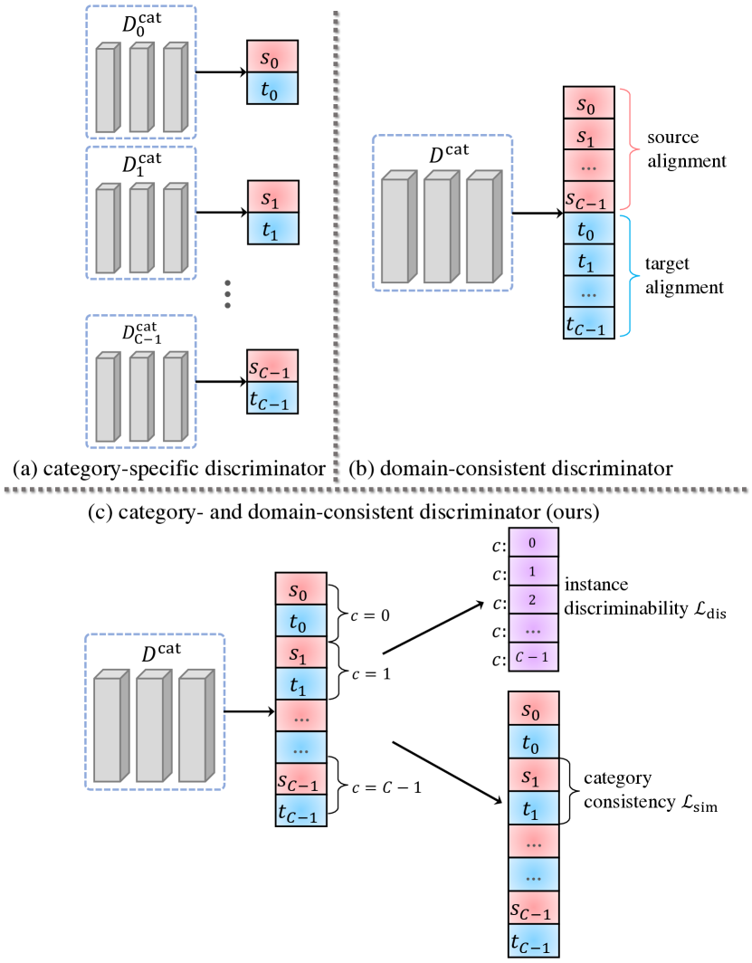
Figure 4: Illustration of different category-level discriminators $D$, where $s_{c}$ and $t_{c}$ denote the $c$-th category ($c=0,1,\cdots,C-1$) in source domain and target domain respectively. (a) Category-specific discriminators for each category [25, 26, 27]. (b) Domain-consistent discriminator to distinguish different categories within one domain [28]. (c) Our category- and domain-consistent discriminator to consider both instance discriminability in different categories and category consistency between two domains.

3.3.2 Category-level Discriminator

In order to keep the semantic consistency between different domain distributions, a category-level discriminator is applied. Previous methods design either category-specific discriminators for each category (e.g., [25, 26, 27], see Figure 4 (a)) or a domain-consistent discriminator to distinguish categories within one domain (e.g., [28], see Figure 4 (b)). By contrast, our approach considers jointly instance discriminability in different categories and category consistency between two domains and introduces a novel category- and domain-consistent discriminator (see Figure 4 (c)). Specifically, in our discriminator, we predict the category and domain labels of pixel $(i,j)$ in each image based on feature map $\hat{M}\in\mathbb{R}^{H\times W\times 2C}$, where $\hat{M}\in\mathbb{R}^{H\times W\times 2C}$ is the output by feeding $M$ to the category-level discriminator, $H$ and $W$ are the height and width respectively, and $2C$ represents the total number of categories for source and target domains.

Since there is no ground-truth to supervise the category-level discriminator, we assign pseudo labels to important samples with high confidence from object detection (see Sec. 3.2). In practice, given a batch of input images, we can output the category probability map $P$ using the object detection heads, and obtain the set $\mathcal{S}$ of pseudo labels by utilizeing the probability threshold $\tau_{\text{prob}}$ and non-maximum suppression (NMS) threshold $\tau_{\text{nms}}$. Then, the instances in different categories are classified by Eq. (9), while the same category in two domains is aligned by Eq. (11), as follows:

• In order to keep instance discriminability in different categories, we separate the category distribution by using the following loss function,

  $$\mathcal{L}_{\text{dis}}=-\frac{1}{|\mathcal{S}|}\sum_{(i,j)\in\mathcal{S}}\sum_{c=0}^{C-1}\hat{y}^{\text{dis}}_{i,j,c}\log(p^{\text{dis}}_{i,j,c}).$$ (9)

  By normalizing confidence over the domain channel, $p_{i,j,c}^{\text{dis}}$ represents the probability of the $c$-th category of the pixel $(i,j)$, i.e.,

  $$\small p^{\text{dis}}_{i,j,c}=\frac{\exp{(\hat{M}_{i,j,2c}+\hat{M}_{i,j,2c+1})}}{\sum_{c=0}^{C-1}\exp{(\hat{M}_{i,j,2c}+\hat{M}_{i,j,2c+1})}},$$ (10)

  where $\hat{M}_{i,j,2c}$ and $\hat{M}_{i,j,2c+1}$ represent the confidence of the $c$-th category in source and target domains, respectively (see again Figure 4(c)). $\hat{y}^{\text{dis}}\in\mathbb{R}^{H\times W\times C}$ is the pseudo category label. We have $\hat{y}^{\text{dis}}_{i,j,c}=1$ if the instance at $(i,j)$ in $\hat{M}$ is an important one of the $c$-th category and $\hat{y}^{\text{dis}}_{i,j,c}=0$ otherwise.

• Category consistency between two domains. After classifying instances of different categories, we need to further identify which domain the instance belongs to. With GRL [14], we write the loss function as follows,

  $$\mathcal{L}_{\text{sim}}=-\frac{1}{|\mathcal{S}|}\sum_{(i,j)\in\mathcal{S}}\sum_{m=0}^{2C-1}\hat{y}^{\text{sim}}_{i,j,m}\log(p^{\text{sim}}_{i,j,m}),$$ (11)

  where $y^{\text{sim}}\in\mathbb{R}^{H\times W\times 2C}$ is the pseudo domain label. Similarly, $\hat{y}^{\text{sim}}_{i,j,m}=1$ if the instance at $(i,j)$ in $\hat{M}$ is an important one of the $\lfloor\frac{m}{2}\rfloor$-th category in specific domain and $\hat{y}^{\text{sim}}_{i,j,m}=0$ otherwise. The domain probability $p^{\text{sim}}$ is obtained as follows,

  $$p^{\text{sim}}_{i,j,m}=\left\{\begin{array}[]{ll}\frac{\exp(\hat{M}_{i,j,m})}{\exp(\hat{M}_{i,j,m-1})+\exp(\hat{M}_{i,j,m})},&{\rm if~{}}m{\rm~{}is~{}odd}\\ \frac{\exp(\hat{M}_{i,j,m})}{\exp(\hat{M}_{i,j,m})+\exp(\hat{M}_{i,j,m+1})}.&{\rm if~{}}m{\rm~{}is~{}even}\end{array}\right.$$ (12)

With the above analysis, we define the final loss function $\mathcal{L}_{\text{cat}}$ for the category-level discriminator $D^{\text{cat}}$ as follows,

$$\mathcal{L}_{\text{cat}}=\lambda_{\text{dis}}\mathcal{L}_{\text{dis}}+\lambda_{\text{sim}}\mathcal{L}_{\text{sim}},$$ (13)

where $\mathcal{L}_{\text{dis}}$ and $\mathcal{L}_{\text{sim}}$ are loss functions for instance discriminability and category consistency as in Eq. (9) and Eq. (11), and $\lambda_{\text{dis}}$ and $\lambda_{\text{sim}}$ are the balancing factors.

3.4 Adaptive Exponential Moving Average (AEMA)

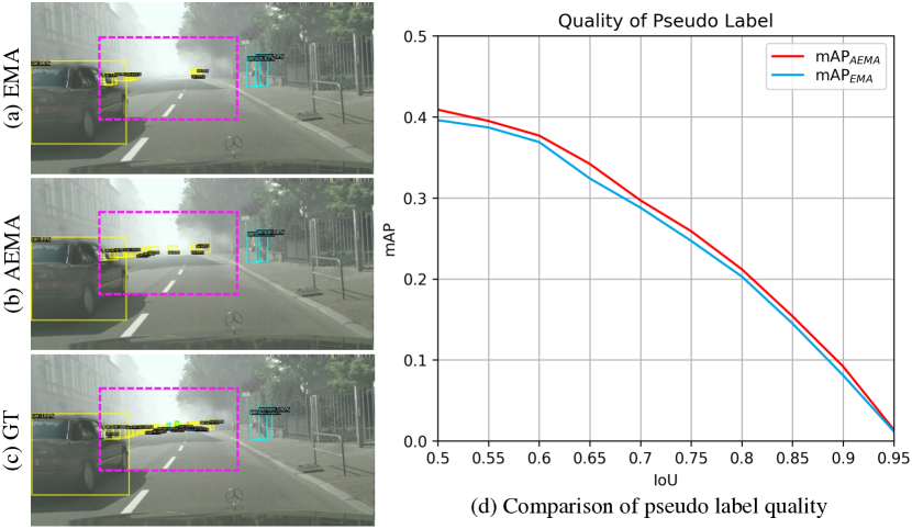
Figure 5: Comparison of the pseudo label quality between EMA and AEMA. Image (a) displays the pseudo label generated by EMA, image (b) the pseudo label by our AEMA, and image (c) the GT pseudo label. In image (d), we demonstrate the mAP scores of the generated pseudo labels of different strategies, and we can observe that AEMA produces better pseudo labels.

As mentioned in Section 3.3.2, the pseudo labels, which are generated by the teacher detector (see Figure 2 (a)), are required for supervising the learning of the category-level discriminator. During the training procedure, the teacher detector is usually updated using exponential moving average (EMA) as follows,

$$\theta_{\mathcal{T}}^{\eta}=(1-\gamma)\cdot\theta_{\mathcal{T}}^{\eta-1}+\gamma\cdot\theta_{\mathcal{S}}^{\eta-1}$$ (14)

where $\theta_{\mathcal{T}}^{\eta}$ represents the weights of the teacher detector at iteration $\eta$, $\theta_{\mathcal{S}}^{\eta-1}$ denotes the weights of the student detector at iteration $\eta-1$, and $\alpha$ is a constant coefficient.

Despite simplicity, the EMA approach may lead to some low-quality pseudo labels (see Figure 5 (a)), because it does not consider the feedback from the two detectors, degrading the final detection performance. To address this problem for improving quality of pseudo labels, we propose an adaptive EMA (AEMA). Specifically, unlike EMA, AEMA considers the intermediate assessments of both teacher and student detectors during update by evaluating their performance on the source domain. Using the assessments as a guidance, an update factor $\delta$ (as described later) is learned to adjust the coefficient $\alpha$ in Eq. (14). More concretely, as in Figure 2, we maintain a memory bank, which is used for generating the assessments. The memory is dynamically updated by storing the images and labels of source domain into it. In order to accurately assess the generalization ability of the detector, we introduce a domain shift simulation (DSS, see Figure. 2 (a)) module, and apply it on the memory bank to generate discrepancy of data distribution on the source domain. Specifically, given the sampling data of images $x^{m}$ and labels $y^{m}$ of all categories from the memory bank, we randomly adjust the mean $x_{u}$ and variance $\sigma^{2}$ of $x^{m}$ to generate the variant data distribution from the source domain, as follows

$$\overline{x}^{m}=\widetilde{\sigma}\frac{x^{m}-x_{u}}{\sqrt{\sigma^{2}+\epsilon}}+\widetilde{x}_{u},$$ (15)

Where the mean $\widetilde{x}_{u}$ and the standard deviation $\widetilde{\sigma}$ for the new variant data distribution are obtained by using the uniform distribution under $x_{u}$ and $\sigma$, respectively, as follows,

$$\widetilde{x}_{u}=U(a_{u},b_{u})x_{u},$$ (16)

$$\widetilde{\sigma}=U(a_{\sigma},b_{\sigma})\sigma,$$ (17)

Here, $U(a,b)$ represents the uniform distribution between $a$ and $b$ and is predefined. Afterwards, the detection losses $\mathcal{L}_{\text{det}}^{\mathcal{T}}$ and $\mathcal{L}_{\text{det}}^{\mathcal{S}}$, obtained by evaluating the teacher and student detectors on the above input date, are employed as the assessment results to derive the update factor $\delta$, as follows,

$$\delta=\begin{cases}e^{\tau_{1}\cdot(0.5-\rho)},\rho<0.5\\ e^{\tau_{2}\cdot(0.5-\rho)},\rho\geq 0.5\end{cases}\;\;\rho=\frac{L_{det}^{\mathcal{S}}}{L_{det}^{\mathcal{S}}+L_{det}^{\mathcal{T}}}$$ (18)

where $\tau_{1}$ and $\tau_{2}$ are two constant values.

Finally, the weights of the teacher detection model can be updated by our AEMA with $\delta$ as follows,

$$\theta_{\mathcal{T}}^{\eta}=(1-\gamma\cdot\delta)\cdot\theta_{\mathcal{T}}^{\eta-1}+\gamma\cdot\delta\cdot\theta_{\mathcal{S}}^{\eta-1}$$ (19)

By using AEMA, we can take into account the assessments of two detectors to guide the update the teacher detection, resulting in better pseudo labels, as shown in Figure 5 (b). Furthermore, we show the statistic comparison of the pseudo labels obtained by teacher detector with EMA and our proposed AEMA in term of accuracy in Figure 5 (d). As demonstrated in Figure 5 (d), we can see that, the quality of the pseudo labels is clearly improved. We will further analyze the effectiveness of our AEMA in later experimental section.

3.5 Overall Loss Function and Optimization

As discussed above, the omni-scale gated object detection network is supervised by $\mathcal{L}_{\text{gui}}$ and $\mathcal{L}_{\text{det}}$. Meanwhile, the multi-granularity discriminators are optimized in different granularities, including pixel-level $\mathcal{L}_{\text{pix}}$, instance-level $\mathcal{L}_{\text{ins}}$ and category-level $\mathcal{L}_{\text{cat}}$. In summary, the overall loss function is defined as

$$\mathcal{L}=(\underbrace{\mathcal{L}_{\text{gui}}+\mathcal{L}_{\text{det}}}_{\text{object detection}})\ +\alpha\underbrace{(\mathcal{L}_{\text{pix}}+\mathcal{L}_{\text{ins}}+\mathcal{L}_{\text{cat}})}_{\text{multi-granularity discriminators}}$$ (20)

where $\alpha$ is the balancing factor between object detection and multi-granularity discriminators.

The training process of our proposed method is divided into two stages. In stage 1 (S1), we train teacher detector by using SGD optimizer and random sampling with Eq. (6) on source domain. Next, in stage 2 (S2), the student detector is optimized by using SDG optimizer and Eq. (20) on source with labels and target domains with pseudo labels, and the teacher detector is updated by adaptive exponential moving average (AEMA).

TABLE I: Results of our approach and comparison to state-of-the-arts on weather adaptation from Cityscapes to FoggyCityscapes. The best two results are highlighted in red and blue fonts, respectively. Note that, MGA-DA [1] is the method from our conference version.

Method	Detector	Backbone	person	rider	car	truck	bus	train	mbike	bicycle	mAP
Baseline	Faster-RCNN	VGG-16	17.8	23.6	27.1	11.9	23.8	9.1	14.4	22.8	18.8
DAF [22]	Faster-RCNN	VGG-16	25.0	31.0	40.5	22.1	35.3	20.2	20.0	27.1	27.6
SC-DA [74]	Faster-RCNN	VGG-16	33.5	38.0	48.5	26.5	39.0	23.3	28.0	33.6	33.8
MAF [75]	Faster-RCNN	VGG-16	28.2	39.5	43.9	23.8	39.9	33.3	29.2	33.9	34.0
SW-DA [15]	Faster-RCNN	VGG-16	29.9	42.3	43.5	24.5	36.2	32.6	30.0	35.3	34.3
DAM [17]	Faster-RCNN	VGG-16	30.8	40.5	44.3	27.2	38.4	34.5	28.4	32.2	34.6
MOTR [76]	Faster-RCNN	ResNet-50	30.6	41.4	44.0	21.9	38.6	40.6	28.3	35.6	35.1
CST [77]	Faster-RCNN	VGG-16	32.7	44.4	50.1	21.7	45.6	25.4	30.1	36.8	35.9
PD [78]	Faster-RCNN	VGG-16	33.1	43.4	49.6	22.0	45.8	32.0	29.6	37.1	36.6
CDN [79]	Faster-RCNN	VGG-16	35.8	45.7	50.9	30.1	42.5	29.8	30.8	36.5	36.6
SFOD-Masoic-Defoggy [80]	Faster-RCNN	VGG-16	34.1	44.4	51.9	30.4	41.8	25.7	30.3	37.2	37.0
ATF [70]	Faster-RCNN	VGG-16	34.6	46.5	49.2	23.5	43.1	29.2	33.2	39.0	37.3
SW-Faster-ICR-CCR [29]	Faster-RCNN	VGG-16	32.9	43.8	49.2	27.2	45.1	36.4	30.3	34.6	37.4
SCL [81]	Faster-RCNN	VGG-16	31.6	44.0	44.8	30.4	41.8	40.7	33.6	36.2	37.9
CFFA [82]	Faster-RCNN	VGG-16	43.2	37.4	52.1	34.7	34.0	46.9	29.9	30.8	38.6
GPA [30]	Faster-RCNN	ResNet-50	32.9	46.7	54.1	24.7	45.7	41.1	32.4	38.7	39.5
SAPNet [23]	Faster-RCNN	VGG-16	40.8	46.7	59.8	24.3	46.8	37.5	30.4	40.7	40.9
DSS [83]	Faster-RCNN	ResNet-50	42.9	51.2	53.6	33.6	49.2	18.9	36.2	41.8	40.9
D-adapt [62]	Faster-RCNN	VGG-16	44.9	54.2	61.7	25.6	36.3	24.7	37.3	46.1	41.3
UMT [84]	Faster-RCNN	VGG-16	56.5	37.3	48.6	30.4	33.0	46.7	46.8	34.1	41.7
MeGA-CDA [46]	Faster-RCNN	VGG-16	37.7	49.0	52.4	25.4	49.2	46.9	34.5	39.0	41.8
CDG [53]	Faster-RCNN	VGG-16	38.0	47.4	53.1	34.2	47.5	41.1	38.3	38.9	42.3
TIA [47]	Faster-RCNN	VGG-16	52.1	38.1	49.7	37.7	34.8	46.3	48.6	31.1	42.3
SDA [85]	Faster-RCNN	VGG-16	38.3	47.2	58.8	34.9	57.7	48.3	35.7	42.0	45.2
TDD [59]	Faster-RCNN	VGG-16	39.6	47.5	55.7	33.8	47.6	42.1	37.0	41.4	43.1
SIGMA [50]	Faster-RCNN	VGG-16	46.9	48.4	63.7	27.1	50.7	35.9	34.7	41.4	43.5
MGA-DA [1]	Faster-RCNN	VGG-16	43.9	49.6	60.6	29.6	50.7	39.0	38.3	42.8	44.3
Baseline (ours)	Faster-RCNN	VGG-16	39.4	46.8	48.2	23.2	36.0	16.8	35.2	43.2	36.1
MGA (ours)	Faster-RCNN	VGG-16	47.0	54.6	64.8	28.5	52.1	41.5	40.9	49.5	47.4
oracle	Faster-RCNN	VGG-16	48.2	53.3	68.5	31.7	55.3	33.1	41.9	49.3	47.7
SST-AL [69]	FCOS	-	45.1	47.4	59.4	24.5	50.0	25.7	26.0	38.7	39.6
CFA [18]	FCOS	VGG-16	41.9	38.7	56.7	22.6	41.5	26.8	24.6	35.5	36.0
SCAN [86]	FCOS	VGG-16	41.7	43.9	57.3	28.7	48.6	48.7	31.0	37.3	42.1
MGA-DA [1]	FCOS	VGG-16	45.7	47.5	60.6	31.0	52.9	44.5	29.0	38.0	43.6
CFA [18]	FCOS	ResNet-101	41.5	43.6	57.1	29.4	44.9	39.7	29.0	36.1	40.2
MGA-DA [1]	FCOS	ResNet-101	43.1	47.3	61.5	30.2	53.2	50.3	27.9	36.9	43.8
Baseline (ours)	FCOS	VGG-16	31.4	31.0	42.7	14.2	26.9	2.3	17.6	31.6	24.7
Baseline (ours)	FCOS	ResNet-101	35.2	37.2	43.5	17.3	31.8	7.2	27.0	34.5	29.2
MGA (ours)	FCOS	VGG-16	47.9	50.1	64.9	34.8	58.0	45.6	38.3	43.7	47.9
MGA (ours)	FCOS	ResNet-101	47.2	48.1	63.7	37.5	54.6	50.8	28.8	44.2	46.9
oracle	FCOS	VGG-16	51.7	48.9	69.5	39.1	52.8	56.0	31.8	40.0	48.7
oracle	FCOS	ResNet-101	46.3	46.0	66.8	38.8	57.3	52.2	36.4	36.9	47.6

4 Experiments

Extension of our framework. Our MGA framework is designed for general purpose and applicable to both one- and two-stage detection models. To verify this, in addition to the representative one-stage FCOS [75], we further extend our MGA to the popular two-stage Faster-RCNN [7] that consists of Region Proposal Network (RPN) and RCNN with classification and regression branches. As shown in Figure 2 (b), we employ RPN as our coarse detection module, whose loss function is replaced by the original RPN loss, i.e., $L_{\text{gui}}=L_{\text{rpn}}$; and we use RCNN as object detection module with the loss defined as $L_{\text{det}}=L_{\text{cls}}+L_{\text{reg}}$. For omni-scale gate fusion, we first obtain the top $K$ proposals by using RPN based on the backbone feature layer with stride 16. Then, we further extract the pixel-level features with low-resolution and high-resolution streams, and generate instance features of $7\times 7$ under the pixel-level feature map and original input feature maps by using the ROIAlign operation. Finally, the instance features are merged according to the RPN outputs and Eq. (5) after using a convolution of $3\times 3$, as shown in Figure 3 (b).

Implementation. In this work, we implement our method based on different detectors (i.e., Faster-RCNN and FCOS) and backbones (i.e., VGG-16 and ResNet-101) using PyTorch [87] to show generality of our approach. Both VGG-16 and ResNet-101 are pre-trained on ImageNet [3]. We utilize a unified optimization framework by using training process of two stages and warm-up followed the previous works [18] and [50] for different detectors. Similar to [23], we apply the Adam optimizer with an initial learning rate of 3e-4, a momentum of 0.9 and weight decay of 1e-4 in Faster-RCNN framework. For FCOS framework, we use SGD optimizer with an initial learning rate of 5e-3, a momentum of 0.9 and weight decay of 1e-4, being consistent with CFA [18]. $\gamma$ is $0.1$ in Eq. (14). The parameters $a_{u}$ and $b_{u}$ are set respectively to $0.4$ and $0.5$ in Eq. (16), and the $a_{\delta}$ and $b_{\delta}$ respectively to $0.8$ and $0.9$ in Eq. (17). The thresholds $\tau_{\text{prob}}$ and $\tau_{\text{nms}}$ for obtaining $\mathcal{S}$ are empirically set to $0.42$ and $0.5$. All our experiments are conducted on the machine with an Intel(R) Xeon(R) CPU and 4 Tesla V100 GPUs. Our code will be made publicly available at https://github.com/tiankongzhang/MGA.

4.1 Datasets

To verify the proposed method, we conduct extensive experiments on different adaption settings, as described below.

Weather adaptation. For weather adaptation, we explore generalization of the detector on Cityscapes [31] and FoggyCityscapes [32]. Cityscapes [31] is a popular street scene dataset with normal weather, which comprises 2,975 training images and 500 validation images. FoggyCityscapes [32] is synthesized on Cityscapes with different levels of fog (i.e., 0.005, 0.01 and 0.02). For fair comparison, we choose the level of $0.02$ for experiment as in other methods in Table I. In weather adaptation, we use Cityscapes [31] as the source domain and FoggyCityscapes [32] as the target domain.

TABLE II: Results of our approach and comparison to state-of-the-arts on real-to-artistic adaptation from PASCAL VOC to Clipart. The best two results are highlighted in red and blue fonts, respectively. Note, there are no oracle results for Clipart because all images in Clipart are used for evaluation.

Method	Detector	Backbone	acro	bicycle	bird	boat	bottle	bus	car	cat	chair	cow
Baseline	Faster-RCNN	ResNet-101	35.6	52.5	24.3	23.0	20.0	43.9	32.8	10.7	30.6	11.7
SW-DA [15]	Faster-RCNN	ResNet-101	26.2	48.5	32.6	33.7	38.5	54.3	37.1	18.6	34.8	58.3
SCL [81]	Faster-RCNN	ResNet-101	44.7	50.0	33.6	27.4	42.2	55.6	38.3	19.2	37.9	69.0
ATF [70]	Faster-RCNN	ResNet-101	41.9	67.0	27.4	36.4	41.0	48.5	42.0	13.1	39.2	75.1
PD [78]	Faster-RCNN	ResNet-101	41.5	52.7	34.5	28.1	43.7	58.5	41.8	15.3	40.1	54.4
SAPNet [23]	Faster-RCNN	ResNet-101	27.4	70.8	32.0	27.9	42.4	63.5	47.5	14.3	48.2	46.1
UMT [58]	Faster-RCNN	ResNet-101	39.1	59.1	32.4	35.0	45.1	61.9	48.4	7.5	46.0	67.6
SFOD-ODS [51]	Faster-RCNN	ResNet-101	43.1	61.4	40.1	36.8	48.2	45.8	48.3	20.4	44.8	53.3
D-adapt [62]	Faster-RCNN	ResNet-101	56.4	63.2	42.3	40.9	45.3	77.0	48.7	25.4	44.3	58.4
MGA-DA [1]	Faster-RCNN	ResNet-101	35.5	64.6	27.8	34.5	41.6	66.4	49.8	26.8	43.6	56.7
Baseline (ours)	Faster-RCNN	ResNet-101	30.5	35.3	24.8	23.5	34.8	65.7	32.6	9.0	35.1	26.4
MGA (ours)	Faster-RCNN	ResNet-101	38.7	77.2	39.0	35.4	53.8	78.1	47.5	17.5	38.2	49.9
			table	dog	horse	bike	person	plant	sheep	sofa	train	tv	mAP
Baseline	Faster-RCNN	ResNet-101	13.8	6.0	36.8	45.9	48.7	41.9	16.5	7.3	22.9	32.0	27.8
SW-DA [15]	Faster-RCNN	ResNet-101	17.0	12.5	33.8	65.5	61.6	52.0	9.3	24.9	54.1	49.1	38.1
SCL [81]	Faster-RCNN	ResNet-101	30.1	26.3	34.4	67.3	61.0	47.9	21.4	26.3	50.1	47.3	41.5
ATF [70]	Faster-RCNN	ResNet-101	33.4	7.9	41.2	56.2	61.4	50.6	42.0	25.0	53.1	39.1	42.1
PD [78]	Faster-RCNN	ResNet-101	26.7	28.5	37.7	75.4	63.7	48.7	16.5	30.8	54.5	48.7	42.1
SAPNet [23]	Faster-RCNN	ResNet-101	31.8	17.9	43.8	68.0	68.1	49.0	18.7	20.4	55.8	51.3	42.2
UMT [58]	Faster-RCNN	ResNet-101	21.4	29.5	48.2	75.9	70.5	56.7	25.9	28.9	39.4	43.6	44.1
SFOD-ODS [51]	Faster-RCNN	ResNet-101	32.5	26.1	40.6	86.3	68.5	48.9	25.4	33.2	44.0	56.5	45.2
D-adapt [62]	Faster-RCNN	ResNet-101	31.4	24.5	47.1	75.3	69.3	43.5	27.9	34.1	60.7	64.0	49.0
MGA-DA [1]	Faster-RCNN	ResNet-101	24.3	20.9	43.2	84.3	74.2	41.1	17.4	27.6	56.5	57.6	44.8
Baseline (ours)	Faster-RCNN	ResNet-101	24.2	12.2	31.2	55.5	40.4	52.2	5.7	18.4	45.0	38.4	32.0
MGA (ours)	Faster-RCNN	ResNet-101	20.0	18.0	44.2	83.5	74.6	57.7	26.7	26.0	55.4	58.3	47.0

TABLE III: Results of our approach and comparison to state-of-the-arts on real-to-artistic adaptation from PASCAL VOC to Watercolor. The best two results are highlighted in red and blue fonts, respectively.

Method	Detector	Backbone	bike	bird	car	cat	dog	person	mAP
Baseline	Faster-RCNN	ResNet-101	68.8	46.8	37.2	32.7	21.3	60.7	44.6
SW-DA [15]	Faster-RCNN	ResNet-101	82.3	55.9	46.5	32.7	35.5	66.7	53.3
SCL [81]	Faster-RCNN	ResNet-101	82.2	55.1	51.8	39.6	38.4	64.0	55.2
ATF [70]	Faster-RCNN	ResNet-101	78.8	59.9	47.9	41.0	34.8	66.9	54.9
PD [78]	Faster-RCNN	ResNet-101	95.8	54.3	48.3	42.4	35.1	65.8	56.9
SAPNet [23]	Faster-RCNN	ResNet-101	81.1	51.1	53.6	34.3	39.8	71.3	55.2
UMT [58]	Faster-RCNN	ResNet-101	88.2	55.3	51.7	39.8	43.6	69.9	58.1
SFOD-ODS [51]	Faster-RCNN	ResNet-101	95.2	53.1	46.9	37.2	47.6	69.3	58.2
AT [60]	Faster-RCNN	ResNet-101	93.6	56.1	58.9	37.3	39.6	73.8	59.9
MGA-DA [1]	Faster-RCNN	ResNet-101	87.6	49.9	56.9	37.4	44.6	72.5	58.1
Baseline (ours)	Faster-RCNN	ResNet-101	76.0	46.7	52.0	27.7	33.3	54.9	48.4
MGA (ours)	Faster-RCNN	ResNet-101	85.3	59.7	59.7	43.3	46.6	77.7	62.1
oracle	Faster-RCNN	ResNet-101	67.1	53.4	43.9	46.3	50.5	79.8	56.8

Cross-Camera adaptation. In Cross-Camera adaptation, we evaluate our algorithm on KITTI [34] and Cityscapes. KITTI [34] is a popular traffic scene dataset containing 7,481 training images. In this adaption experiment, KITTI is the source domain and Cityscapes is the target domain. Following previous works [81, 50], we only report the results on the category of car.

Synthetic-to-Real adaptation. For Synthetic-to-Real adaptation, we utilize SIM10k [33] and Cityscapes for experiments. SIM10k [33] is a synthetic scene dataset from the game video Grand Theft Auto V (GTA5). It contains 10k training images, and we conduct comparisons on the car class, similar to [81]. In this adaptation experiment, we utilize the SIM10k as the source domain and Cityscapes as the target domain.

Real-to-Artistic adaptation. In Real-to-Artistic adaptation, we verify our method on PASCAL VOC [35], Clipart [36] and Watercolor [36] datasets. PASCAL VOC [35] is a real-scene dataset including two sub-datasets (i.e., PASCAL VOC 2007 and PASCAL VOC 2012). PASCAL VOC 2007 consists of 2,501 images for training and 2,510 images for validation, and PASCAL VOC 2012 contains 5,717 images for training and 5,823 mages for validation. Clipart [36] is a carton dataset with 1k images and has the same categories as PASCAL VOC. Watercolor [36] is a watercolor style dataset containing 1,000 training images and 1,000 testing images, and it shares 6 classes with PASCAL VOC. In this setting, we use PASCAL VOC as the source domain and Clipart or Watercolor as the target domain.

4.2 State-of-the-Art Comparison

Figure 6: Qualitative results and comparison (from left column to right column: weather adaptation from Cityscapes to FoggyCityscapes, real-to-artistic adaptation from PASCAL VOC to Clipart and Watercolor, cross-camera adaption from Kitti to Cityscapes, and synthetic-to-real adaption from SIM10k to Cityscapes). We can see that MGA achieves superior results than MGA-DA in our conference version and the baseline method.

TABLE IV: Results of our approach and comparison to state-of-the-arts on cross-camera/synthetic-to-real adaptation detection results from Kitti/SIM10k to Cityscapes. The best two results are highlighted in red and blue fonts, respectively.

Method	Detector	Backbone	AP${}_{\text{car}}$
Baseline	Faster-RCNN	VGG-16	30.2/30.1
DAF [22]	Faster-RCNN	VGG-16	38.5/39.0
MAF [75]	Faster-RCNN	VGG-16	41.0/41.1
ATF [70]	Faster-RCNN	VGG-16	42.1/42.8
SC-DA [74]	Faster-RCNN	VGG-16	42.5/43.0
UMT [84]	Faster-RCNN	VGG-16	-/43.1
SFOD-Mosaic [80]	Faster-RCNN	VGG-16	44.6/43.1
CST [77]	Faster-RCNN	VGG-16	43.6/44.5
MeGA-CDA [46]	Faster-RCNN	VGG-16	43.0/44.8
SAPNet [23]	Faster-RCNN	VGG-16	43.4/44.9
CDN [79]	Faster-RCNN	VGG-16	44.9/49.3
TIA [47]	Faster-RCNN	VGG-16	44.0/  –
DSS [83]	Faster-RCNN	ResNet-50	42.7/44.5
SSD [88]	Faster-RCNN	ResNet-50	47.6/49.3
SIGMA [50]	Faster-RCNN	VGG-16	45.8/53.7
TDD [59]	Faster-RCNN	VGG-16	47.4/53.4
MGA-DA [1]	Faster-RCNN	VGG-16	45.2/49.8
Baseline (ours)	Faster-RCNN	VGG-16	43.7/44.1
MGA (ours)	Faster-RCNN	VGG-16	54.3/55.5
oracle	Faster-RCNN	VGG-16	68.1
SST-AL [69]	FCOS	-	45.6/51.8
CFA [86]	FCOS	VGG-16	43.2/49.0
SCAN [86]	FCOS	VGG-16	45.8/52.6
CFA [18]	FCOS	ResNet-101	45.0/51.2
MGA-DA [1]	FCOS	VGG-16	48.5/54.6
MGA-DA [1]	FCOS	ResNet-101	46.5/54.1
Baseline (ours)	FCOS	VGG-16	43.1/43.0
Baseline (ours)	FCOS	ResNet-101	41.3/43.7
MGA (ours)	FCOS	VGG-16	49.9/55.8
MGA (ours)	FCOS	ResNet-101	47.6/55.4
oracle	FCOS	VGG-16	73.4
oracle	FCOS	ResNet-101	71.8

In this section, we demonstrate our results and comparison with state-of-the-art methods using different base detectors (i.e., Faster-RCNN [7] and FCOS [8]) and backbones (i.e., VGG-16 [4] and ReseNet-101 [2]) on different adaptation scenarios. In all comparison table, “Baseline (ours)” means that the baseline detector is equipped with our OSGF and trained using data augmentation as in our method but without adaption strategy, and “oracle” indicates that the baseline detector is trained and tested on the target domain without any adaptation strategy.

Weather adaptation. In Table I, we report the results from Cityscapes to FoggyCityscapes. As displayed in Table I, for Faster-RCNN detector, our method achieves the best mAP of $47.4\%$ and outperforms the second best SDA [85] with $45.2\%$ mAP by $2.4\%$. Compared to the baseline (ours) of $36.1\%$, MGA obtains $11.3\%$ performance gains. For FCOS detector, we also obtain the best mAP scores of $47.9\%$ with VGG-16 and $46.9\%$ with ResNet-101. Compared with the approaches of SCAN [86] with VGG-16 and CFA [18] with ResNet-101, our MGA respectively shows the $5.8\%$ and $6.7\%$ gains. In addition, our method observes obvious improvements over the baseline (ours) with 23.2% using VGG-16 and 17.7% gains using ResNet-101, which verifies the effectiveness of our method. Furthermore, compared with MGA-DA [1] with 44.3% mAP score for Fatser-RCNN and 43.6% and 43.8 % mAP scores for FCOS on VGG-16 and ResNet-101 backbone in our conference version, our MGA shows 3.1%, 4.3% and 3.1% gains, showing the effectiveness of our new contributions.

Real-to-Artistic adaptation. Table II and III show the results and comparison in real-to-artistic adaptation. As in Table II, from PASCAL VOC to Clipart, our method achieves the second mAP score of $47.0\%$, and D-adapt [62] obtains the best performance of $49.0\%$. Compared to our baseline, we achieve $15.0\%$ performance gain. In Table III, our MGA performs the best with $62.1\%$ mAP score and surpasses the second best AT [60] with $59.9\%$ by $2.2\%$. Besides, our method outperforms the oracle, indicating that our MGA makes full use of the information between source and target domains for robust UDA detection.

Cross-Camera adaptation. Table IV displays the results and comparison from Kitti to Cityscapes. As shown in Table IV, on Faster-RCNN detector, our method shows the best result of $54.3\%$ AP${}_{\text{car}}$ with VGG-16. In contrast to the baseline (ours), we obtain $10.6\%$ gain. Using FCOS detector, our MGA outperforms SCAN [86] by $4.1\%$ with VGG-16 and CFA [18] by $2.6\%$ with ResNet-101. Compared to the baseline (ours), MGA obtains $6.8\%$ and $6.3\%$ performance gains with VGG-16 and ResNet-101, respectively, showing its advantages.

Synthetic-to-Real adaptation. Table IV shows the result from Sim10k to Cityscapes. On Faster-RCNN detector, our MGA achieves the best result of $55.5\%$ AP${}_{\text{car}}$. In contrast to the baseline (ours), it obtains a $11.4\%$ gain. On FCOS detector, our method shows the best AP${}_{\text{car}}$ of $55.8\%$ with VGG-16 and $55.4\%$ with ResNet-101. In comparison with SCAN [86] with VGG-16 and CFA [18] with ResNet-101, we obtains $3.2\%$ and $4.2\%$ gains with VGG-16 and ResNet-101, respectively. Compared to baselines (ours), it demonstrates gains of $12.8\%$ and $11.7\%$ with VGG-16 and ResNet-101, respectively.

Besides quantitative results, we demonstrate qualitative results our method and comparison to other approaches in Figure 6. From Figure 6, we can observe that MGA achieves superior detection results than MGA-DA in our conference version and the baseline method.

4.3 Ablation Study

To further analyze our approach, we conduct ablation experiments on different components. The results are reported under the weather adaptation.

Effectiveness of different components. In order to further validate the effectiveness of different components including omni-scale gated fusion (OSGF), multi-granularity discriminators (MGD) and adaptive exponential moving average (AEMA) in MGA, we demonstrate the results by gradually adding them to the baseline, which is FCOS with VGG16. Table V shows the results. As shown in Table V, with our OSGF, the performance of the baseline is improved from 22.0% to 24.7% with a gain of 2.7%, showing the effectiveness of OSGF in discriminative representation learning. When employing the proposed MGD for adaption, we achieve significant improvement by boosting the result from 24.7% to 45.3% with a 20.6%, which clearly evidences the effectiveness of our method. Further, when adopting AEMA for better pseudo labels, the final result is improved from 45.3% to 47.9%.

Comparison of category-level discriminators. As displayed in the Table VI, we compare our category-level discriminator $D^{\text{cat}}$ and other related class-level discriminators, including $D^{\text{cen}}$ [86], $D^{\text{grp}}$ [26] and $D^{\text{cls}}$ [28] using FCOS with VGG16. The “baseline” indicates that the detector is learned under all strategies but the class-level discriminator is removed from MGA module. $D^{\text{cen}}$ focuses on reducing the differences on the center-aware distributions of source and target domains, which is composed of features of the central positions of objects. $D^{\text{grp}}$ aligns the feature distributions by building a sole domain discriminator for each category. $D^{\text{cls}}$ simultaneously takes domain and class information and expands the binary domain labels by inserting the binary class labels.

TABLE V: Effectiveness of different components.

OSGF	MGD	AEMA	mAP
			22.0
✓			24.7
✓	✓		45.3
✓	✓	✓	47.9

TABLE VI: Comparison between different category-level discriminators.

discriminator	baseline	$D^{\text{cen}}$	$D^{\text{grp}}$	$D^{\text{cls}}$	$D^{\text{cat}}$ (ours)
mAP	44.7	46.2	46.0	45.2	47.9

TABLE VII: Comparison between different fusion methods for OSGF.

S1	S2	w/o OSGF	Conv fusion	Average fusion	Gated fusion (ours)
✓		22.0	23.2	22.8	24.7
✓	✓	45.6	46.2	45.1	47.9

TABLE VIII: Comparison of different OSGF in this work (i.e., OSGF (ours)) and conference version (i.e., OSGF (conference)) [1]. The backbone of the detectors in this table is VGG16.

method	detector	# Params (M)	S1	S1&S2
OSGF (conference) [1]	FCOS	17	23.4	46.8
OSGF (ours)	FCOS	14	24.7	47.9
OSGF (conference) [1]	Faster-RCNN	55	33.8	46.1
OSGF (ours)	Faster-RCNN	50	36.1	47.4

From Table VI, we obverse that the performance of detector is improved from 44.7% to 46.2%/46.0%/45.2% with 1.5%/1.3%/0.5% gains by $D^{\text{cen}}$/$D^{\text{grp}}$/$D^{\text{cls}}$ over the baseline. In contrast, our $D^{\text{cat}}$ improves the baseline detector performance from 44.7% to 47.9%, which shows 3.2% performance gains over the baseline and outperforms other three category-level discriminators by $1.7\%$, $1.9\%$ and $2.7\%$, respectively, evidencing the effectiveness of our approach.

Analysis on gated fusion. In this paper, we introduce a novel gated fusion approach for improved discriminative feature representation. In order to further analyze the gated fusion, we compare it with other commonly used fusion strategies including Conv fusion and Average fusion in Table VII using FCOS with VGG16. In Table VII, “w/o OSGF” means that the OSGF module is removed from our method. “Conv fusion” indicates the fusion weights in OSGF are obtained by using $1\times 1$ convolution, and “Average fusion” means averaging features of convolution kernels in OSGF. From Table VII, we can observe that, in S1, all three fusion methods can improve the performance. In specific, the OSGF with our gated fusion strategy improves the mAP score from 22.0% to 24.7% with 2.7% performance gains, outperforming those using Conv and Average fusion methods with 23.2% and 22.8% mAP scores. Likewise, in S2, OSGF with our gated fusion achieves the best performance, evidencing the effectiveness of gated mechanism for representation learning.

In addition, from Table VIII, we can observe that the improved OSGF in this work contains less parameters and meanwhile achieves better performance compared to that in the preliminary conference version [1], which indicates the advantages of our improved OSGF.

TABLE IX: Comparison between EMA and AEMA for detection performance.

EMA	AEMA	mAP
		45.3
✓		46.5
	✓	47.9

TABLE X: Comparison of computational complexity. The backbone of the detectors in this table is VGG16.

method	detector	# Total Params (M)	FPS
CFA [18]	FCOS	177	17.5
MGA (ours)	FCOS	429	9.1
SCL [81]	Faster-RCNN	580	11.8
SAPNet [23]	Faster-RCNN	556	25.2
MGA (ours)	Faster-RCNN	535	11.0

Comparison of EMA and AEMA. To show the effectiveness of our proposed AEMA, we compare it with EMA using FCOS with VGG16 as shown in Table IX. From Table IX, we obverse that EMA brings in a 1.2% performance gain by improving the result from 45.3% to 46.5%. However, when using the proposed AEMA, the performance is improved to 47.9% with 2.6% gains, which demonstrates the superiority of our AEMA in learning better pseudo labels for detection.

Computational complexity. In Table X, we show the comparison of computational complexity between our method and other state-of-the-art approaches. As shown in Tab. X, on FCOS, our MGA performs better with reasonable increased complexity over its primary contender CFA [18]; while our method has less parameters on the top of Faster-RCNN than two recent methods SCL [81] and SAPNet [23].

5 Conclusion

In this paper, we propose a novel unified multi-granularity alignment (MGA) framework, which encodes dependencies among different pixel-, instance-, and category-levels to achieve alignment of feature distributions for unsupervised domain adaptive detection. Notably, we design the omni-scale gated fusion module with different scales and aspect rations to extract discriminative instance-level feature representation. In order to improve the quality of pseudo labels and mitigate the local misalignment problem in our MGA framework, we further propose a simple but effective dynamic adaptive exponential moving average strategy. Extensive experiments evidence the effectiveness and superiority of our MGA on different detectors for unsupervised domain adaptive object detection.

References

- [1] W. Zhou, D. Du, L. Zhang, T. Luo, and Y. Wu, “Multi-granularity alignment domain adaptation for object detection,” in CVPR, 2022.
- [2] K. He, X. Zhang, S. Ren, and J. Sun, “Deep residual learning for image recognition,” in CVPR, 2016.
- [3] A. Krizhevsky, I. Sutskever, and G. E. Hinton, “Imagenet classification with deep convolutional neural networks,” NIPS, 2012.
- [4] K. Simonyan and A. Zisserman, “Very deep convolutional networks for large-scale image recognition,” in ICLR, 2015.
- [5] R. Girshick, J. Donahue, T. Darrell, and J. Malik, “Rich feature hierarchies for accurate object detection and semantic segmentation,” in CVPR, 2014.
- [6] R. Girshick, “Fast r-cnn,” in ICCV, 2015.
- [7] S. Ren, K. He, R. B. Girshick, and J. Sun, “Faster R-CNN: towards real-time object detection with region proposal networks,” TPAMI, vol. 39, no. 6, pp. 1137–1149, 2017.
- [8] Z. Tian, C. Shen, H. Chen, and T. He, “FCOS: fully convolutional one-stage object detection,” in ICCV, 2019.
- [9] H. Law and J. Deng, “Cornernet: Detecting objects as paired keypoints,” in ECCV, 2018.
- [10] W. Liu, D. Anguelov, D. Erhan, C. Szegedy, S. Reed, C.-Y. Fu, and A. C. Berg, “Ssd: Single shot multibox detector,” in ECCV, 2016.
- [11] J. Redmon, S. Divvala, R. Girshick, and A. Farhadi, “You only look once: Unified, real-time object detection,” in CVPR, 2016.
- [12] T.-Y. Lin, P. Dollár, R. Girshick, K. He, B. Hariharan, and S. Belongie, “Feature pyramid networks for object detection,” in CVPR, 2017.
- [13] T.-Y. Lin, M. Maire, S. Belongie, J. Hays, P. Perona, D. Ramanan, P. Dollár, and C. L. Zitnick, “Microsoft coco: Common objects in context,” in ECCV, 2014.
- [14] Y. Ganin and V. S. Lempitsky, “Unsupervised domain adaptation by backpropagation,” in ICML, 2015.
- [15] K. Saito, Y. Ushiku, T. Harada, and K. Saenko, “Strong-weak distribution alignment for adaptive object detection,” in CVPR, 2019.
- [16] E. Tzeng, J. Hoffman, K. Saenko, and T. Darrell, “Adversarial discriminative domain adaptation,” in CVPR, 2017.
- [17] T. Kim, M. Jeong, S. Kim, S. Choi, and C. Kim, “Diversify and match: A domain adaptive representation learning paradigm for object detection,” in CVPR, 2019.
- [18] C. Hsu, Y. Tsai, Y. Lin, and M. Yang, “Every pixel matters: Center-aware feature alignment for domain adaptive object detector,” in ECCV, 2020.
- [19] H.-K. Hsu, C.-H. Yao, Y.-H. Tsai, W.-C. Hung, H.-Y. Tseng, M. Singh, and M.-H. Yang, “Progressive domain adaptation for object detection,” in WACV, 2020.
- [20] Q. Cai, Y. Pan, C.-W. Ngo, X. Tian, L. Duan, and T. Yao, “Exploring object relation in mean teacher for cross-domain detection,” in CVPR, 2019.
- [21] Z. He and L. Zhang, “Multi-adversarial faster-rcnn for unrestricted object detection,” in ICCV, 2019.
- [22] Y. Chen, W. Li, C. Sakaridis, D. Dai, and L. V. Gool, “Domain adaptive faster R-CNN for object detection in the wild,” in CVPR, 2018.
- [23] C. Li, D. Du, L. Zhang, L. Wen, T. Luo, Y. Wu, and P. Zhu, “Spatial attention pyramid network for unsupervised domain adaptation,” in ECCV, 2020.
- [24] X. Zhu, J. Pang, C. Yang, J. Shi, and D. Lin, “Adapting object detectors via selective cross-domain alignment,” in CVPR, 2019.
- [25] L. Du, J. Tan, H. Yang, J. Feng, X. Xue, Q. Zheng, X. Ye, and X. Zhang, “SSF-DAN: separated semantic feature based domain adaptation network for semantic segmentation,” in ICCV, 2019.
- [26] L. Hu, M. Kan, S. Shan, and X. Chen, “Unsupervised domain adaptation with hierarchical gradient synchronization,” in CVPR, 2020.
- [27] S. Paul, Y. Tsai, S. Schulter, A. K. Roy-Chowdhury, and M. Chandraker, “Domain adaptive semantic segmentation using weak labels,” in ECCV, 2020.
- [28] H. Wang, T. Shen, W. Zhang, L. Duan, and T. Mei, “Classes matter: A fine-grained adversarial approach to cross-domain semantic segmentation,” in ECCV, 2020.
- [29] C. Xu, X. Zhao, X. Jin, and X. Wei, “Exploring categorical regularization for domain adaptive object detection,” in CVPR, 2020.
- [30] M. Xu, H. Wang, B. Ni, Q. Tian, and W. Zhang, “Cross-domain detection via graph-induced prototype alignment,” in CVPR, 2020.
- [31] M. Cordts, M. Omran, S. Ramos, T. Rehfeld, M. Enzweiler, R. Benenson, U. Franke, S. Roth, and B. Schiele, “The cityscapes dataset for semantic urban scene understanding,” in CVPR, 2016.
- [32] C. Sakaridis, D. Dai, and L. V. Gool, “Semantic foggy scene understanding with synthetic data,” IJCV, vol. 126, no. 9, pp. 973–992, 2018.
- [33] M. Johnson-Roberson, C. Barto, R. Mehta, S. N. Sridhar, K. Rosaen, and R. Vasudevan, “Driving in the matrix: Can virtual worlds replace human-generated annotations for real world tasks?” in ICRA, 2017.
- [34] A. Geiger, P. Lenz, and R. Urtasun, “Are we ready for autonomous driving? the KITTI vision benchmark suite,” in CVPR, 2012.
- [35] M. Everingham, L. V. Gool, C. K. I. Williams, J. M. Winn, and A. Zisserman, “The pascal visual object classes (VOC) challenge,” IJCV, vol. 88, no. 2, pp. 303–338, 2010.
- [36] N. Inoue, R. Furuta, T. Yamasaki, and K. Aizawa, “Cross-domain weakly-supervised object detection through progressive domain adaptation,” in CVPR, 2018.
- [37] J. Redmon and A. Farhadi, “Yolo9000: better, faster, stronger,” in CVPR, 2017.
- [38] J. Dai, Y. Li, K. He, and J. Sun, “R-fcn: Object detection via region-based fully convolutional networks,” NIPS, 2016.
- [39] K. He, G. Gkioxari, P. Dollár, and R. Girshick, “Mask r-cnn,” in ICCV, 2017.
- [40] T.-Y. Lin, P. Goyal, R. Girshick, K. He, and P. Dollár, “Focal loss for dense object detection,” in ICCV, 2017.
- [41] S. Zhang, L. Wen, X. Bian, Z. Lei, and S. Z. Li, “Single-shot refinement neural network for object detection,” in CVPR, 2018.
- [42] Z. Cai and N. Vasconcelos, “Cascade r-cnn: Delving into high quality object detection,” in CVPR, 2018.
- [43] K. Duan, S. Bai, L. Xie, H. Qi, Q. Huang, and Q. Tian, “Centernet: Keypoint triplets for object detection,” in ICCV, 2019.
- [44] N. Carion, F. Massa, G. Synnaeve, N. Usunier, A. Kirillov, and S. Zagoruyko, “End-to-end object detection with transformers,” in ECCV, 2020.
- [45] A. Vaswani, N. Shazeer, N. Parmar, J. Uszkoreit, L. Jones, A. N. Gomez, Ł. Kaiser, and I. Polosukhin, “Attention is all you need,” NIPS, 2017.
- [46] V. VS, V. Gupta, P. Oza, V. A. Sindagi, and V. M. Patel, “Mega-cda: Memory guided attention for category-aware unsupervised domain adaptive object detection,” in CVPR, 2021.
- [47] L. Zhao and L. Wang, “Task-specific inconsistency alignment for domain adaptive object detection,” in CVPR, 2022.
- [48] C. Chen, J. Li, Z. Zheng, Y. Huang, X. Ding, and Y. Yu, “Dual bipartite graph learning: A general approach for domain adaptive object detection,” in ICCV, 2021.
- [49] M. Xu, H. Wang, B. Ni, Q. Tian, and W. Zhang, “Cross-domain detection via graph-induced prototype alignment,” in CVPR, 2020.
- [50] W. Li, X. Liu, and Y. Yuan, “Sigma: Semantic-complete graph matching for domain adaptive object detection,” in CVPR, 2022.
- [51] S. Li, M. Ye, X. Zhu, L. Zhou, and L. Xiong, “Source-free object detection by learning to overlook domain style,” in CVPR, 2022.
- [52] M. Khodabandeh, A. Vahdat, M. Ranjbar, and W. G. Macready, “A robust learning approach to domain adaptive object detection,” in ICCV, 2019.
- [53] S. Li, J. Huang, X.-S. Hua, and L. Zhang, “Category dictionary guided unsupervised domain adaptation for object detection,” in AAAI, 2021.
- [54] M. Chen, W. Chen, S. Yang, J. Song, X. Wang, L. Zhang, Y. Yan, D. Qi, Y. Zhuang, D. Xie et al., “Learning domain adaptive object detection with probabilistic teacher,” in ICML, 2022.
- [55] F. Yu, D. Wang, Y. Chen, N. Karianakis, T. Shen, P. Yu, D. Lymberopoulos, S. Lu, W. Shi, and X. Chen, “Sc-uda: Style and content gaps aware unsupervised domain adaptation for object detection,” in WACV, 2022.
- [56] C. Chen, Z. Zheng, X. Ding, Y. Huang, and Q. Dou, “Harmonizing transferability and discriminability for adapting object detectors,” in CVPR, 2020.
- [57] Z. Shen, M. Huang, J. Shi, Z. Liu, H. Maheshwari, Y. Zheng, X. Xue, M. Savvides, and T. S. Huang, “Cdtd: A large-scale cross-domain benchmark for instance-level image-to-image translation and domain adaptive object detection,” IJCV, vol. 129, no. 3, pp. 761–780, 2021.
- [58] J. Deng, W. Li, Y. Chen, and L. Duan, “Unbiased mean teacher for cross-domain object detection,” in CVPR, 2021.
- [59] M. He, Y. Wang, J. Wu, Y. Wang, H. Li, B. Li, W. Gan, W. Wu, and Y. Qiao, “Cross domain object detection by target-perceived dual branch distillation,” in CVPR, 2022.
- [60] Y.-J. Li, X. Dai, C.-Y. Ma, Y.-C. Liu, K. Chen, B. Wu, Z. He, K. Kitani, and P. Vajda, “Cross-domain adaptive teacher for object detection,” in CVPR, 2022.
- [61] W. Ren, L. Ma, J. Zhang, J. Pan, X. Cao, W. Liu, and M. Yang, “Gated fusion network for single image dehazing,” in CVPR, 2018.
- [62] J. Jiang, B. Chen, J. Wang, and M. Long, “Decoupled adaptation for cross-domain object detection,” in ICLR, 2022.
- [63] T. Chen, S. Kornblith, K. Swersky, M. Norouzi, and G. E. Hinton, “Big self-supervised models are strong semi-supervised learners,” NeurIPS, 2020.
- [64] Z. Cai, A. Ravichandran, S. Maji, C. Fowlkes, Z. Tu, and S. Soatto, “Exponential moving average normalization for self-supervised and semi-supervised learning,” in CVPR, 2021.
- [65] A. Islam, C.-F. R. Chen, R. Panda, L. Karlinsky, R. Feris, and R. J. Radke, “Dynamic distillation network for cross-domain few-shot recognition with unlabeled data,” NeurIPS, 2021.
- [66] M. Xu, Z. Zhang, H. Hu, J. Wang, L. Wang, F. Wei, X. Bai, and Z. Liu, “End-to-end semi-supervised object detection with soft teacher,” in ICCV, 2021.
- [67] Q. Yang, X. Wei, B. Wang, X.-S. Hua, and L. Zhang, “Interactive self-training with mean teachers for semi-supervised object detection,” in CVPR, 2021.
- [68] T. Lin, P. Dollár, R. B. Girshick, K. He, B. Hariharan, and S. J. Belongie, “Feature pyramid networks for object detection,” in CVPR, 2017.
- [69] M. A. Munir, M. H. Khan, M. S. Sarfraz, and M. Ali, “Synergizing between self-training and adversarial learning for domain adaptive object detection,” in NeurIPS, 2021.
- [70] Z. He and L. Zhang, “Domain adaptive object detection via asymmetric tri-way faster-rcnn,” in ECCV, 2020.
- [71] H. Rezatofighi, N. Tsoi, J. Gwak, A. Sadeghian, I. D. Reid, and S. Savarese, “Generalized intersection over union: A metric and a loss for bounding box regression,” in CVPR, 2019.
- [72] J. Yu, Y. Jiang, Z. Wang, Z. Cao, and T. S. Huang, “Unitbox: An advanced object detection network,” in ACM MM, 2016.
- [73] T. Lin, P. Goyal, R. B. Girshick, K. He, and P. Dollár, “Focal loss for dense object detection,” in ICCV, 2017.
- [74] X. Zhu, J. Pang, C. Yang, J. Shi, and D. Lin, “Adapting object detectors via selective cross-domain alignment,” in CVPR, 2019.
- [75] Z. He and L. Zhang, “Multi-adversarial faster-rcnn for unrestricted object detection,” in ICCV, 2019.
- [76] Q. Cai, Y. Pan, C. Ngo, X. Tian, L. Duan, and T. Yao, “Exploring object relation in mean teacher for cross-domain detection,” in CVPR, 2019.
- [77] G. Zhao, G. Li, R. Xu, and L. Lin, “Collaborative training between region proposal localization and classification for domain adaptive object detection,” in ECCV, 2020.
- [78] A. Wu, Y. Han, L. Zhu, and Y. Yang, “Instance-invariant domain adaptive object detection via progressive disentanglement,” TPAMI, 2021.
- [79] P. Su, K. Wang, X. Zeng, S. Tang, D. Chen, D. Qiu, and X. Wang, “Adapting object detectors with conditional domain normalization,” in ECCV, 2020.
- [80] X. Li, W. Chen, D. Xie, S. Yang, P. Yuan, S. Pu, and Y. Zhuang, “A free lunch for unsupervised domain adaptive object detection without source data,” in AAAI, 2021.
- [81] Z. Shen, H. Maheshwari, W. Yao, and M. Savvides, “SCL: towards accurate domain adaptive object detection via gradient detach based stacked complementary losses,” CoRR, vol. abs/1911.02559, 2019.
- [82] Y. Zheng, D. Huang, S. Liu, and Y. Wang, “Cross-domain object detection through coarse-to-fine feature adaptation,” in CVPR, 2020.
- [83] Y. Wang, R. Zhang, S. Zhang, M. Li, Y. Xia, X. Zhang, and S. Liu, “Domain-specific suppression for adaptive object detection,” in CVPR, 2021.
- [84] J. Deng, W. Li, Y. Chen, and L. Duan, “Unbiased mean teacher for cross-domain object detection,” in CVPR, 2021.
- [85] Q. Zhou, Q. Gu, J. Pang, Z. Feng, G. Cheng, X. Lu, J. Shi, and L. Ma, “Self-adversarial disentangling for specific domain adaptation,” arXiv, 2021.
- [86] W. Li, X. Liu, X. Yao, and Y. Yuan, “Scan: Cross domain object detection with semantic conditioned adaptation,” in AAAI, 2022.
- [87] A. Paszke, S. Gross, F. Massa, A. Lerer, J. Bradbury, G. Chanan, T. Killeen, Z. Lin, N. Gimelshein, L. Antiga et al., “Pytorch: An imperative style, high-performance deep learning library,” NeurIPS, 2019.
- [88] F. Rezaeianaran, R. Shetty, R. Aljundi, D. O. Reino, S. Zhang, and B. Schiele, “Seeking similarities over differences: Similarity-based domain alignment for adaptive object detection,” in ICCV, 2021.