EvidenceCap: Towards trustworthy medical image segmentation via evidential identity cap

Abstract

Medical image segmentation (MIS) is essential for supporting disease diagnosis and treatment effect assessment. Despite considerable advances in artificial intelligence (AI) for MIS, clinicians remain skeptical of its utility, maintaining low confidence in such black box systems, with this problem being exacerbated by low generalization for out-of-distribution (OOD) data. To move towards effective clinical utilization, we propose a foundation model named EvidenceCap, which makes the box transparent in a quantifiable way by uncertainty estimation. EvidenceCap not only makes AI visible in regions of uncertainty and OOD data, but also enhances the reliability, robustness, and computational efficiency of MIS. Uncertainty is modeled explicitly through subjective logic theory to gather strong evidence from features. We show the effectiveness of EvidenceCap in three segmentation datasets and apply it to the clinic. Our work sheds light on clinical safe applications and explainable AI, and can contribute towards trustworthiness in the medical domain.

1 Introduction

As a result of extensive research into deep learning, medical image segmentation using Convolutional Neural Networks (CNNs) has greatly facilitated quantitative pathological assessments [1, 2], diagnostic support systems [3, 4, 5] and tumor analysis [6, 7]. Nonetheless, clinicians still question the capabilities of artificial intelligence (AI), viewing it as a black box. This doubt is manifested in clinicians preferring not to use AI-derived results as a basis for making informed decisions [8, 9]. This situation is exacerbated by AI being prone to prediction vulnerability that yields unreliable results, especially with out-of-distribution (OOD) data [10]. These limitations prompted us to introduce EvdenceCap, a new paradigm for trustworthy medical image segmentation, which acts like an out-of-the-box identity cap that can quantify what was hitherto a black box (Fig. 1 a).

Researchers have focused on modifying deep network structures for improving the accuracy of segmentation in the last decade. Fully Convolutional Networks (FCN) has been developed to achieve end-to-end accurate semantic segmentation with notable results [11]. The U-Net [12] model and its variants [13, 14, 15, 16] were then proposed to obtain better feature representations and segmentation results. Highly expressive Transformers [17, 18, 19] have also been used with great success in computer vision and medical image segmentation. Nonetheless, it is not enough to obtain accurate segmentation results. In particular,
-The above medical image segmentation methods have limited versatility. Due to OOD data, medical image segmentation performance may drop significantly after deployment to real systems [10]. Therefore, the awareness of OOD data of the real environment is very important for the deployed system. After all, it is very time-consuming to re-collect, label and train data for the current system.
-Current medical image segmentation methods ignore the situations that AI may make ambiguous decisions. In clinical practice, there are often situations where AI decisions may be not well-informed, and principled mechanisms for quantifying uncertainty are required for clinically-safe applications [8]. Knowing the unknowns of predictions while delivering accurate and robust performance will help foster trust in AI technologies among clinicians. Therefore, uncertainty estimation is an effective way to promote trustworthy decisions.

Existing uncertainty estimation methods remain poorly utilized in medical image segmentation. Uncertainty quantification methods in medical domain include Bayesian-[20], ensemble-[21], evidential-[22], and deterministic-based methods[23, 24]. A simple way to produce uncertainty for medical image segmentation is to use an ensemble of deep networks [25, 26]. However, deep ensembles require retraining the model from scratch, which incurs a high computation cost for complex models. Some methods introduce the dropout in the test phase to estimate lesion-level Bayesian uncertainties [27, 28, 29]. Although this strategy reduces the computational burden, it leads to inconsistent outputs [30]. Deep deterministic uncertainty [31] is extended for semantic segmentation using feature space densities. Unfortunately, the above methods inevitably change the network structure and incur computational costs. A recent study has proposed using a deep feature-extraction module and an evidential layer to segment lymphomas from positron emission tomography and computed tomography image [22]. The main aims of these studies remained on guiding uncertainty to improve segmentation performance rather than obtaining more robust segmentation with calibrated uncertainty, and on generating uncertainty to evaluate the segmentation results rather than utilizing the calibrated uncertainty to further optimize the model training. What’s more, there is no sufficient clinically applicable diagnostic studies using uncertainty estimation to allow AI to filter out low-quality samples and alert OOD data.

Trustworthy, robust, and computationally efficient uncertainty estimations provide visible quality assessments for clinical practice. The main objective of this study is to introduce trustworthy medical image segmentation and demonstrate its potential in clinical applications. We develop a trustworthy medical image segmentation framework named EvidenceCap, which works like an identity cap that provides robustness, confidence, and high efficiency for medical image segmentation. EvidenceCap renders the output of the underlying network in an evidence-level manner. This not only estimates a stable and reasonable pixel-level uncertainty, but also improves the reliability and robustness of segmentation. EvidenceCap derives probabilities and uncertainties for different class segmentation problems via Subjective Logic (SL) theory, where the Dirichlet distribution parameterizes the distribution of probabilities for different classes of the segmentation results. Moreover, EvidenceCap is uncertain for inaccurate segmented regions during initial training, while remaining confident for accurate regions during subsequent training. To reiterate, EvidenceCap can be flexibly applied to any segmentation backbone without incurring heavy implementation and excessive computational burden. EvidenceCap can be applied to detect OOD data and indicate image data quality. We demonstrate here that EvidenceCap achieves a superior performance with potential ease of interpretation in medical image segmentation for diagnostic support and quantitative assessments of diseases.

2 Results

EvidenceCap pipeline & trustworthy medical image segmentation.

EvidenceCap is a trustworthy medical image segmentation framework based on evidential deep learning, which provides robust segmentation performance and reliable uncertainty quantification for diagnostic support. A pipeline of EvidenceCap and its results in undertaking trustworthy medical image segmentation tasks are shown in Fig. 1 b and c. In the training phase (Fig. 1 b), EvidenceCap can be applied to any task in numerous medical domains. Its trained model visually generates auxiliary diagnostic results, including robust target segmentation results and reliable uncertainty estimation. In the testing phase, in order to verify the effectiveness of the method, EvidenceCap was tested for confidence, robustness, and computational efficiency on different segmentation tasks.

To illustrate, three challenging trustworthy medical image segmentation tasks using different datasets are undertaken here: (1) dermoscopic images in a 2D setting using the ISIC2018 dataset; (2) liver CT images in a 3D setting using the LiTS2017 dataset; and (3) multi-modality MRI images in a multi-modality 3D setting using the BraTS2019 dataset. In the first task, we hope to use robust segmentation performance and reliable uncertainty quantification in evaluating skin lesions. In the second task, we hope to obtain credible 3D segmentations for the liver. In the third task, we hope to obtain robust segmentation results and credible uncertainty estimations for brain tumors under extreme conditions. A detailed description of the three tasks is presented in App. 1. Trustworthy medical image segmentation tasks.. We hope to show through successful completion of these tasks that segmentation results with uncertainty estimations of different models on different datasets can contribute to credible disease diagnosis and treatment effect assessment through medical images.

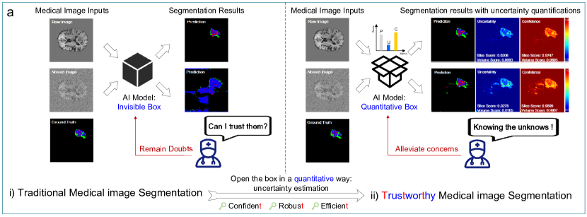
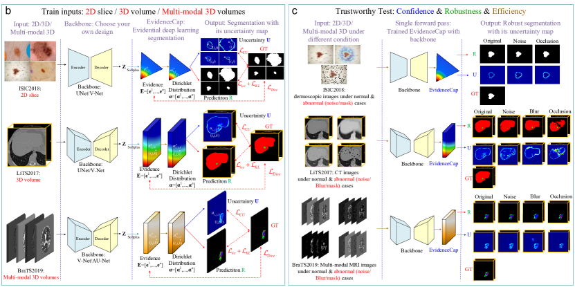
Figure 1: a. The motivation for trustworthy medical image segmentation, i) Traditional medical image segmentation; ii) Trustworthy medical image segmentation. b. The training process of our framework. c. The trustworthy test on three datasets. R, U, and GT denote the prediction, uncertainty map, and ground truth, respectively.

Task 1: EvidenceCap for skin lesion segmentation.

AI makes it possible for dermatologists to quickly diagnose and screen for early stages of skin diseases using skin lesion boundary segmentation [32, 33]. However, there have been few studies on skin lesion segmentation with noise interference. As such, we conducted studies at different levels of Gaussian noise and random masking based on the ISIC2018 dataset (2D dermoscopic image) to validate the robustness of our proposed framework.
Comparison with U-Net based methods. We compared the results with EvidenceCap with those of other U-Net variants at differing Gaussian noise with variance ${\sigma^{2}}=\left\{0.1,0.2,0.3,0.4,0.5\right\}$ and different mask ratios (MR) $MR=\left\{0.1,0.25,0.4\right\}$ with eight patch-size (Fig. 2 a). Performance with U-Net and V-Net degrades slowly, especially at higher masking ratios and noise, as these confound AI. After applying EvidenceCap, the results gain partial immunity to interference (Fig. 2 b). The basic network after applying EvidenceCap contains some anti-interference ability, and the visual uncertainty estimation graph generated can alert researchers and clinicians to the unreliability of data.
Comparison with uncertainty-based methods. We compared our framework with uncertainty-based algorithms and found the PU to be significantly disturbed by noise and masking, while the underlying network after applying EvidenceCap shows less perturbations (Fig. 2 a). Comparison of the uncertainty estimation results by ECE and UEO metrics show that the backbone networks obtained a more robust uncertainty estimation ability after applying EvidenceCap. Our visualization of the segmentation results and uncertainty estimates (Fig. 2 b) indicated that the addition of our framework provides higher uncertainty for target edges and the noised or masked pixels, suggesting that our framework can alert researchers and clinicians to OOD data.

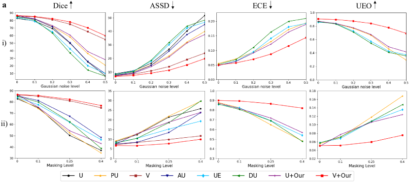
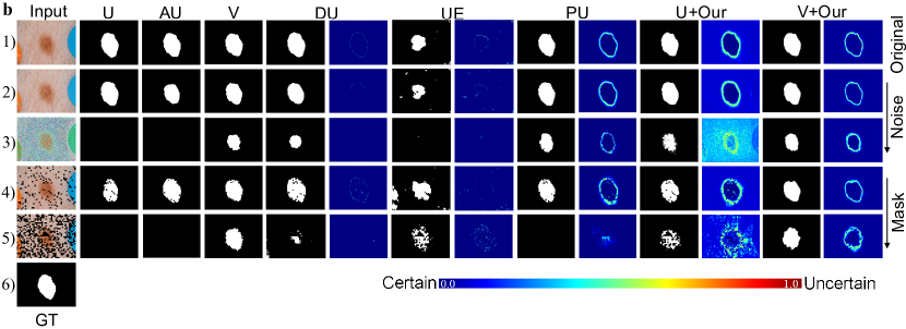
Figure 2: a. Quantitative comparisons of U-Net based methods and uncertainty-based methods using the ISIC2018 dataset under differing Gaussian noise ($\sigma^{2}=\left\{{0,0.1,0.2,0.3,0.4,0.5}\right\}$) and patch-size mask degradation ($MR=\left\{{0,0.1,0.25,0.4}\right\}$): i) Dice, ASSD, ECE and UEO metrics at differeing Gaussian noise i) the same metrics at differing masking ratios. b. Visual comparison of skin lesion segmentation results with different methods: 1) original input and its results; (2-3) input with Gaussian noise ($\sigma^{2}=0.2,0.5$) and its results; (4-5) input with patch-size random mask ($\sigma^{2}=0.1,0.4$) and its results; (6) ground truth.

Task 2: EvidenceCap for liver segmentation.

AI can assist clinicians in hepatocellular carcinoma diagnosis and treatment planning for liver cancers [34]. To verify the reliability and robustness of our method, we conducted studies with the Liver2017 dataset (3D CT) under differing levels of Gaussian noise, Gaussian blur, and random masking to achieve trustworthy medical image segmentation.
Comparison with U-Net based methods. To verify the robustness of EvidenceCap, we compared other U-Net-based methods using differing Gaussian noise with variance ${\sigma^{2}}=\left\{0.05,0.1,0.2,0.3,0.4\right\}$, differing Gaussian blur with variance
$\left\{{\left({{\sigma^{2}},k}\right)}\right\}=\left\{{\left({{\rm{11,10}}}\right),\left({{\rm{13,10}}}\right),\left({{\rm{15,20}}}\right),\left({{\rm{23,20}}}\right)}\right\}$, and differing masking ratios (MR) $MR=\left\{{0,0.1,0.25,0.4}\right\}$ with eight patch-size. We found the results of U-Net based methods to gradually decrease in four metrics with an increase in OOD, but this can be suppressed when EvidenceCap is applied (Fig. 3 a). The robustness of the base method equipped with EvidenceCap is higher than those of other methods, as indicated by our method segmentation results with their uncertainty map under differing conditions (Fig. 3 b). Our framework also provides uncertainty maps that allow further diagnosis and analysis.
Comparison with uncertainty-based methods. We repeated the study with uncertainty-based algorithms to further compare the calibrated uncertainty for segmentation. Performance in uncertainty estimation for all methods degrades with increasing Gaussian noise, Gaussian blur, and random masking (Fig. 3 a). However, the backbones equipped with EvidenceCap mitigates this degradation. Under normal conditions, our framework provides higher uncertainty for liver edges compared to other methods. Under OOD conditions, our framework is more sensitive to unseen regions and provides high uncertainty (Fig. 3 b). EvidenceCap thus allows clinicians or annotators to better focus on areas of uncertainty in order to work more efficiently.

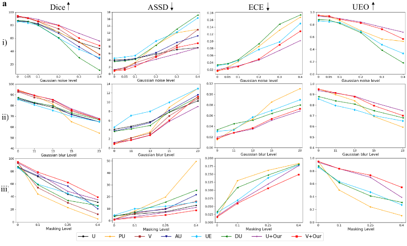
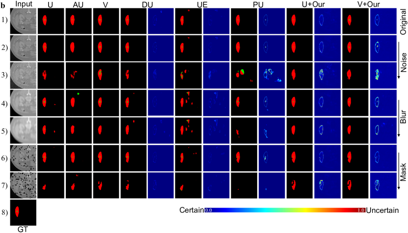
Figure 3: a. Quantitative comparisons of U-Net based methods and uncertainty-based methods with the Liver2017 dataset under differing Gaussian noise, Gaussian blur, and patch-size random masking degradation conditions: i) Dice, ASSD, ECE, and UEO metrics at differing Gaussian noise $\sigma^{2}=\left\{{0,0.05,0.1,0.2,0.3,0.4}\right\}$; ii) four metrics at differing Gaussian blur $\left\{{\left({{\sigma^{2}},k}\right)}\right\}=\left\{{\left({{\rm{11,10}}}\right),\left({{\rm{13,10}}}\right),\left({{\rm{15,20}}}\right),\left({{\rm{23,20}}}\right)}\right\}$; iii) four metrics at differing random masking $MR=\left\{{0.1,0.25,0.4}\right\}$. b. Visual comparison of liver segmentation results using different methods: a) original input and its results; (b-c) input with Gaussian noise ($\sigma^{2}=0.2,0.4$) and its results; (d-e) input with Gaussian blur ($\left\{{\left({{\sigma^{2}},k}\right)}\right\}=\left\{{\left({{\rm{13,10}}}\right),\left({{\rm{15,20}}}\right)}\right\}$) and its results; (f-g) Input with random mask ratios ($\sigma^{2}=0.1,0.4$) and its results; (h) ground truth.

Task 3: EvidenceCap for brain tumor segmentation.

AI can allow for the accurate segmentation of brain tumor from different imaging modalities to assess the effectiveness pre- and post-treatment. We conducted studies using the BraTS2019 dataset (3D multi-modality MRI) with differing levels of Gaussian noise, Gaussian blur, and random masking to achieve trustworthy medical image segmentation.
Comparison with U-Net based methods. To verify the robustness of our model, we vary Gaussian noise with variance ${\sigma^{2}}=\left\{0.5,1.0,1.5,2.0\right\}$, Gaussian blur with variance
$\left\{{\left({{\sigma^{2}},k}\right)}\right\}=\left\{{\left({{\rm{3,3}}}\right),\left({{\rm{5,5}}}\right),\left({{\rm{7,7}}}\right),\left({{\rm{9,9}}}\right)}\right\}$, and masking ratios (MR) $MR=\left\{0.1,0.25,0.4,0.6\right\}$ with eight patch-size to the voxels of the four modalities (Fig. 4 a). We observe that without EvidenceCap, V-Net and Attention-UNet show results comparable to those of other methods, but performance decreases rapidly with additional conditions. V-Net and Attention-UNet with our framework perform more robustly under increased conditioned levels (Fig. 4 b).
Comparison with uncertainty-based methods. To further quantify the reliability of the uncertainty estimation, we compared our model to different uncertainty-based methods, using the elegant uncertainty evaluation metrics of ECE and UEO. The performances of all uncertainty-based methods decay gradually with increasing levels of Gaussian noise (Figs. 4 a (2)-(4)), but our method decays more slowly with the benefit of the reliable and robust evidences captured by our trusted segmentation framework. Visually comparing brain tumor segmentation results from different methods to demonstrate the reliability of the uncertainty estimations, the V-Net and Attention-UNet with EvidenceCap applied obtained more accurate and robust uncertainty estimations, even under strong noised conditions (Fig. 4 b). This is due to our not using softmax for output which would lead to over-confidence [23]; instead, we employed a subjective logical framework to gather more favorable and robust evidence from the data.

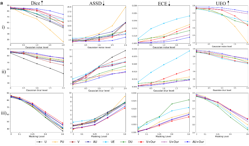
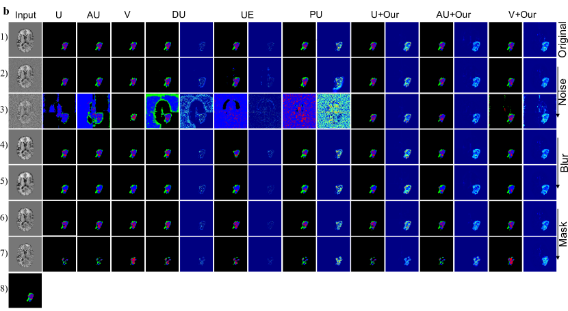
Figure 4: a. Quantitative comparisons with U-Net based methods and uncertainty-based methods with the BraTS2019 dataset under differing Gaussian noise ( $\sigma^{2}=\left\{{0.5,1.0,1.5,2.0}\right\}$), Gaussian blur ($\left\{{\left({{\sigma^{2}},k}\right)}\right\}=\left\{{\left({{\rm{3,3}}}\right),\left({{\rm{5,5}}}\right),\left({{\rm{7,7}}}\right),\left({{\rm{9,9}}}\right)}\right\}$) and patch-size mask degradation conditions ($MR=\left\{{0.1,0.25,0.4,0.6}\right\}$: i) Dice, ASSD, ECE, and UEO metrics with differing Gaussian noise; ii) the same metrics with differing Gaussian blur; iii) The same metrics of different masking ratios. b.The visual comparison of brain tumor segmentation results with different methods. 1) Original input (T2 as an example); 2)-3) Gaussian noise input under ($\sigma^{2}=\left\{1.0,2.0\right\}$) and its results; 4)-5) Input under Gaussian blur ($\left\{{\left({{\sigma^{2}},k}\right)}\right\}=\left\{{\left({{\rm{3,3}}}\right),\left({{\rm{7,7}}}\right)}\right\}$) and its results; 6)-7) input under random mask ratio $MR=\left\{{0.1,0.4}\right\}$ and its results; 8) ground truth.

Inference analysis of uncertainty estimation models for the three tasks.

DU [35] applied Monte-Carlo dropout ($p$=0.5) on U-Net before pooling or after upsampling. UE [21] quantifies the uncertainties by ensembling multiple models. UE shares the same U-Net structure and trained with different random initialization on the different subsets (90%) of the training dataset to enhance variability. PU [30] learns a conditional density model over-segmentation based on a combination of a U-Net with a conditional variational autoencoder. The methods described above modify the original network structure or reduce the efficiency of training. Our method explicitly quantifies the uncertainty with a single forward pass through the backbone neural network using subjective logic theory. To demonstrate the effectiveness of the efficiency (computational cost and accuracy), we provide more insight into the performances of uncertainty estimation methods on the datasets of ISIC2018, LiTS2017, and BraTS2019 with Gaussian noise by ${\sigma^{2}}{\rm{=}}\left\{{0.3,0.2,1.5}\right\}$ (Tab. 1). The backbones (U/AU/V) applying EvidenceCap considerably outperformed the baseline uncertainty quantification methods in testing time and FLOPs (Tab. 1). This is because our method avoids changing the network structure and incurs lower computational costs. Moreover, our method achieves better performance on Dice score, Average Symmetric Surface Distance (ASSD), Expected Calibration Error (ECE), and Uncertainty-error overlap (UEO), especially in the case of high noise interference. In contrast, both DU [35] and UE [21] give unsatisfactory results, especially under high noise conditions. PU [30] improves on these results, but still struggles to maintain performance under high noise conditions. This is because PU and DU will sample at the point of testing to obtain uncertainty estimations, and the UE obtains uncertainty estimations by ensembling multiple models. The success of EvidenceCap is attributed to employing the subjective logical framework to gather strong evidence from the data. Additionally, it does not use the softmax layer for output, avoiding over-confidence in the process. EvidenceCap develops a supervised strategy for uncertainty estimation to guarantee better performance and calibrated uncertainty.

Table 1: Inference analysis of Uncertainty estimation models on above three datasets under normal condition and Gaussian noise condition (${\sigma^{2}}{\rm{=}}0.3,0.3,1.5$). N and OOD denote the normal condition and out-of-distribution condition, respectively.

	Methods	Testing time$\downarrow$	Parameter$\downarrow$	FLOPs$\downarrow$	Dice$\uparrow$		ASSD$\downarrow$		ECE$\downarrow$		UEO$\uparrow$
					N	OOD	N	OOD	N	OOD	N	OOD
ISIC2018	UE [21]	57.34 s	7.77 M	137.34 G	0.839	0.425	8.28	30.20	0.049	0.142	0.858	0.416
	DU [35]	26.16 s	7.77 M	137.34 G	0.849	0.369	8.06	31.78	0.052	0.163	0.865	0.544
	PU [30]	0.14 s	27.35 M	108.54 G	0.837	0.580	9.19	21.87	0.055	0.130	0.878	0.665
	U+Ours	0.07 s	7.77 M	13.74 G	0.868	0.530	7.41	21.47	0.048	0.119	0.871	0.650
	V+Ours	0.08 s	13.07 M	15.45 G	0.874	0.781	6.71	11.35	0.045	0.087	0.905	0.839
LiTS2017	UE [21]	230.22 s	4.75 M	776.04 G	0.856	0.603	4.57	9.58	0.031	0.077	0.858	0.647
	DU [35]	204.24 s	4.75 M	776.04 G	0.874	0.607	3.65	8.35	0.034	0.093	0.880	0.670
	PU [30]	1.32 s	5.13 M	157.46 G	0.938	0.690	0.92	8.45	0.017	0.086	0.941	0.703
	U+Ours	0.73 s	4.75 M	77.60 G	0.933	0.800	1.27	4.29	0.020	0.047	0.935	0.842
	V+Ours	0.35 s	2.31 M	48.01 G	0.944	0.797	0.93	4.41	0.017	0.049	0.949	0.825
BraTS2019	UE [21]	195.48 s	4.76 M	6941.65 G	0.857	0.709	3.42	4.93	0.0091	0.0211	0.857	0.727
	DU [35]	105.90 s	4.76 M	6941.65 G	0.825	0.662	2.50	5.79	0.0062	0.0104	0.855	0.697
	PU [30]	15.4 s	5.13 M	1423.74 G	0.864	0.470	1.63	10.02	0.0058	0.0143	0.886	0.622
	U+Ours	2.40 s	4.76 M	1263.69 G	0.850	0.743	2.89	4.74	0.0058	0.0088	0.864	0.838
	AU+Ours	2.72 s	4.77 M	1285.60 G	0.859	0.803	1.89	2.25	0.0054	0.0071	0.880	0.845
	V+Ours	1.71 s	2.31 M	790.16 G	0.870	0.721	1.58	4.10	0.0048	0.0127	0.895	0.761

Clinically safe applications: out-of-distribution detector & Image quality indicator

Out-of-distribution detector: EvidenceCap distinguishes OOD data for medical applications. It is essential that image processing systems identify any OOD samples in clinical settings. Uncertainty estimation quantifies the uncertainty of the in-distribution and OOD data to detect inputs that are far outside the training data distribution. EvidenceCap can thus be used to alert clinicians to areas where lesions may be present in OOD data. We conducted OOD experiments on the Johns Hopkins OCT dataset and Duke OCT dataset with Diabetic Macular Edema (DME). The specific experimental details can be found in the App. 3. Experimental details of Clinically safety applications.. We found significant differences in the uncertainty results of the in-distribution and OOD data (Fig. 5 a), with the uncertainty values of some regions with DME lesions increasing significantly (Fig. 5 a (ii)). There are also marked differences in the uncertainty of predictions between the in-distribution and OOD (Fig. 5 b). These results combine to show that EvidenceCap provides a solution for filtering out abnormal areas where lesions may be present in OOD data. In this way, this ensures that downstream models are only run on in-distribution data that are likely to perform well, facilitating diagnostic analysis of clinical data.
Image quality indicator: EvidenceCap indicates the quality of medical images. As medical data fuels the use of AI in medicine, it is crucial to accurately quantify the value of data in algorithmic prediction and decision-making. Uncertainty estimation is an intuitive and quantitative way to inform clinicians or researchers about the quality of medical images. EvidenceCap guides image quality quantitatively through the distribution of uncertainty values and qualitatively through the degree of explicitness of the uncertainty map. This is due to the significant difference in uncertainty values between high-quality and low-quality data sources. In what follows, we apply EvidenceCap to indicate the quality of data for real-world applications. The Digital Retinal Images for Vessel Extraction (DRIVE) and the Fundus Image Vessel Segmentation (FIVES) datasets are used for quality assessment experiments. The experimental details can be found in the App. 3. Experimental details of Clinically safety applications.. As the image quality decreases, the change in the uncertainty map becomes more evident (Fig. 5 c). We also found differences in the uncertainty distribution of high and low-quality of images (Fig. 5 d (1)). The uncertainty sensitivity curve is designed to quantify the quality of data (Fig. 5 d (2)). It shows the uncertainty value-ratio at different uncertainty thresholds. The lower the uncertainty threshold, the higher the uncertainty value-ratio should be. These results demonstrate that EvidenceCap can serve as an image quality indicator to fairly value personal data in healthcare and consumer markets. This would help to remove harmful data while identifying and collecting higher-value data for diagnostic support.

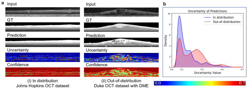
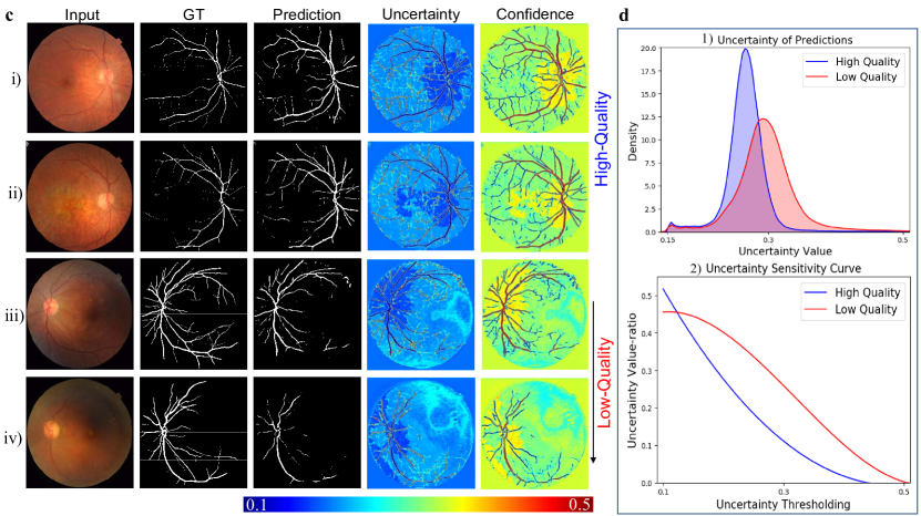
Figure 5: Clinically safety applications for out-of-distribution detector and quality indicator. a. The qualitative difference between in-distribution (Johns Hopkins dataset without disease) and out-of-distribution data (Duke dataset with DME). DME: diabetic macular edema. b. The quantified difference in uncertainty distribution of in-distribution and out-of-distribution data. c. Qualitative differences between image data of differing qualities. i-ii) Visualization results of high-quality data on the FIVES dataset. iiii-iv) Low-quality data visualization results on the FIVES dataset. d. Quantitative difference in uncertainty distribution and uncertainty sensitivity curve for images of different qualities. 1) Density of uncertainty of predictions for different quality data. 2) Uncertainty sensitivity curve on the different quality data.

3 Discussion

Although medical image segmentation methodology is growing considerably, this has not been matched by a corresponding increase in reliability and robustness [36]. Developing a reliable method for medical image segmentation is one solution to this issue that provides sensitivity and explicability for OOD data. In this study, we develop EvidenceCap, the first reliable medical image segmentation method which works as an identity cap for backbone networks to generate robust segmentation results and credible uncertainty estimations. We performed three trustworthy medical image segmentation tasks using three public datasets, namely ISIC2018 (2D settings), LiTS2017 (3D settings), and BraTS2019 (Multi-modal 3D settings) respectively, obtaining robust performance and credible uncertainty in each case. We are confident that our work can potentially benefit researchers in the trustworthy medical domain.

Robustness. Robustness is a key feature in trustworthy medical image segmentation. Robustness to adversarial perturbations of the input data is critical to the stability of deep learning [37]. To verify EvidenceCap’s robustness, we studied different imaging modalities in 2D, 3D and multi-modality 3D under different noised conditions using three datasets. The robust performance of the basic network framework (U/V/AU) is significantly improved after applying EvidenceCap (Figure  2, 3 and 4). This performance improvement can possibly be due the trustworthy loss function prompting the network to improve accuracy when beginning training, and then focusing on uncertain regions as learning progresses, rather than in overly skewing segmentation accuracy. EvidenceCap uses a subjective logic framework to gather more evidence from the input data, so as to lead the final opinions.

Confidence. Credibility is another key feature in trustworthy medical image segmentation. Despite recent improvements in the accuracy of medical image segmentation, clinicians still display little confidence towards this technology. A major reason is for clinicians to more likely trust intuitive visualizations. To bridge this gap, EvidenceCap provides pixel-level uncertainty estimations for clinicians while maintaining robustness. We also performed experiments using three datasets to show calibrated uncertainty under different conditions. We found EvidenceCap to provide better uncertainty estimates from the more intuitive cases (Figures 2, 3 and 4). EvidenceCap thus provides clinicians with sufficient visual affirmation in diagnosing and quantitatively assess diseases. By excluding a softmax layer, we avoid assigning over-confident scores for incorrect segmentation results; this avoidance is further aided by the calibrated uncertainty estimation loss function. Of course, the most important is the subjective logic theory, which provides backbones with more evidence to assist the final opinion.

Efficient inference. Execution efficiency is a necessary feature of trustworthy medical image segmentation. To this end, we studied the inference analysis of uncertainty estimation models. EvidenceCap does not visibly change the underlying network structure compared to the DU, UE, and PU methods. We added little to the network parameters while maintaining robustness and calibrated uncertainty (Tab. 1). This is mainly because EvidenceCap does not require multiple sampling like DU and PU, nor does it require ensemble learning like UE to estimate uncertainty. EvidenceCap provides reliability and robustness in processing OOD samples without excessive computational burdens and modifications of the backbone network.

Differences. We analyzed differences in trusted segmentation networks between the traditional medical image segmentation methods [38, 39] and the evidential deep learning method [24]. Compared with the traditional segmentation methods [33, 34, 38, 39], we treat the predictions of the backbone neural network as subjective opinions instead of using a softmax layer to generate predictions with over-confident scores. As a result, our model provides voxel-wise uncertainty estimations and robust segmentations of the medical image, which is essential for facilitating interpretation during disease diagnosis. Applying the evidential deep learning method [24], we develop an evidential deep segmentation framework for use across any backbone network, focusing on trusted medical image segmentation and providing uncertainty estimations for 2D slices and 3D volumes. We adopt the calibrated uncertainty supervision strategy in method training to obtain more accurate and certain predictions.

Invisible box to quantitative box. The studies described above have verified the robustness, trust and high computational efficiency for medical image segmentation provided by EvidenceCap. EvidenceCap converts AI technology from a black box to a system that is quantifiable. Traditional medical image segmentation methods achieve high numerical performances by training UNet and its variants, and are susceptible to fluctuations in the OOD data. Because of this, they are regarded as invisible black boxes. EvidenceCap achieves robust and accurate performance while providing pixel-level confidence. Moreover uncertainty is a quantifiable indicator that can be used as the loss function to design AI models, since it is expected to decrease during training. In addition, the change of uncertainty at the pixel level reflects the reliability of the data, which is more sensitive to OOD data. This helps clinicians in clinical safety applications.

Clinical safety Applications. Finally, we use EvidenceCap in two real-world clinical safety applications. The first application used EvidenceCap as an identification tool for OOD data in the medical domain, which assists clinicians in being more sensitive to abnormal data. We conducted qualitative and quantitative experiments using the Johns Hopkins OCT dataset and Duke OCT dataset with DME. Experimental results showed that EvidenceCap can be used to screen out OOD inputs that may appear to be lesions. The second application used EvidenceCap as a medical image quality diagnostic tool for clinicians to filter unreliable data. By the way, we designed the uncertainty sensitivity curve to better visualize the quality of data. Qualitative and quantitative experiments using the DRIVE and FIVES datasets demonstrate that EvidenceCap can discriminate the quality of data.

Limitations. Although EvidenceCap performs promisingly for segmentation of normal data, there remains room for improvement. Flaws remain when processing high-level OOD data for clinical needs. Multi-modality MRI are directly utilized in task 3 as inputs for segmentation, but we do not progress to estimate uncertainty between the different modalities. Despite this, EvidenceCap provides a reliable shortcut to medical image segmentation for any backbone network through furnishing robust segmentation results with a visible uncertainty map for clinicians and researchers. Looking ahead, there is a need to improve the performance of robust segmentation results and uncertainty estimates under normal and different levels of OOD data. At the same time, further exploration of multi-modal trustworthy medical image segmentation is also needed, as is uncertainty estimation under federated learning. All of these will lead to more trustworthy AI systems for disease diagnosis and treatment.

In conclusion, our foundation model is analyzed and empirically demonstrated through EvidenceCap in this study, paving the way for trustworthy medical image segmentation that generates robust segmentation results and credible uncertainty estimations. Our unified framework for trusted medical image segmentation reduces excessive both computational burden and modifications to the backbone network for a model with evidence. We additionally developed an uncertainty supervised strategy to generate more calibrated uncertainty and maintain the segmentation performance of the base network. We evaluated the robustness and ease of interpretation for data generated by EvidenceCap with three public datasets consisting of different data modalities and different target structures. Our proposed foundation model can apply for two real-world clinical safety applications.

4 Methods

For trustworthy medical image segmentation, we adopted the U-Net [12] and its variants [16, 15] as the backbone networks to obtain the multi-class segmentation results. We did not use softmax as the output layer, as using the largest softmax output leads to over-confidence. As such, we considered the Dirichlet distribution to provide more trusted segmentation results [24]. We further introduced SL [40] to induce probabilities and uncertainties for different classes of segmentation problems. To deal with the unknown pixels in medical images, we propose a calibrated uncertainty strategy for medical image segmentation problem. Finally, we designed the overall loss function for trustworthy medical image segmentation.

4.1 Constructing EvidenceCap

Backbone. U-Net [12] and its variants [16, 15] have seen recent widespread used across medical image modalities. We thus employed them as our backbone for capturing contextual information. Furthermore, the backbones only performed down-sampling three times to reduce information loss and to achieve a balance between GPU memory usage and segmentation accuracy. EvidenceCap can freely choose different backbones to extract image features. We only use its decoder output feature vector without the softmax layer. For a random image $X$ in a medical image domain $\mathbb{X}$, this process can be defined as:

$${{\bf{Z}}_{X}}={f_{\omega}}\left(X\right)$$ (1)

Where ${f_{\omega}}\left(\cdot\right)$ is the different network backbone without the softmax layer. In this study, we assessed the performance of the three general backbones (U-Net [12], V-Net [16] and Attention-UNet [15]).
Dirichlet distribution for medical image segmentation. For typical medical image segmentation tasks [33, 34, 38], the predictions are usually carried by the softmax layer as the final layer. As mentioned in [23, 41], the softmax layer has a tendency to display high confidence even for wrong predictions. EvidenceCap alleviates this problem in the following way: first, the traditional neural network output is followed by an activation function (Softplus) layer to ensure that the network output is non-negative, which is regarded as the evidence voxel ${{\bf{E}}_{X}}=softplus\left({{{\bf{Z}}_{X}}}\right)$. We then obtain a Dirichlet distribution from the network output, which is considered as the conjugate prior of the multinomial distribution [40]. This provides a predictive distribution for medical image segmentation and derives uncertainty from this distribution. For a random image $X$ in a medical image domain $\mathbb{X}$ ($\forall X\in\mathbb{X}$), the projected probability distribution of multinomial opinions is defined by:

$$\boldsymbol{p}_{X}=\boldsymbol{b}_{X}+\boldsymbol{r}_{X}\boldsymbol{U}_{X},$$ (2)

where ${b}_{X}$, $\boldsymbol{r}_{X}$ and $\boldsymbol{U}_{X}$ are the belief mass distribution, base rate distribution and the uncertainty mass distribution over $\mathbb{X}$, respectively. Then, Dirichlet PDF $D({{\boldsymbol{p}}_{X}}\mid{{\bf{\alpha}}_{X}})$ can be used to represent probability density over ${{\boldsymbol{p}}_{X}}$, which is given by:

$$D({{\bf{p}}_{X}}\mid{{\bf{\alpha}}_{X}})=\left\{{\begin{array}[]{*{20}{l}}{\frac{1}{{B({{\bf{\alpha}}_{\bf{X}}})}}\prod\limits_{c=1}^{C}{{{\left({p_{X}^{c}}\right)}^{\alpha_{X}^{c}-1}}}}&{{\rm{for}}\quad{{\bf{p}}_{X}}\in{S_{C}}}\\ 0&{{\rm{otherwise}}}\end{array}}\right.,$$ (3)

where Dirichlet distribution with parameters ${{\bf{\alpha}}_{X}}=\left[{\alpha_{X}^{1},\ldots,\alpha_{X}^{C}}\right]$ is considered as belief mass assignment. $B({\bf{\alpha}_{X}})$ is the $C$-dimensional multinomial beta function, and $S_{C}$ is the C-dimensional unit simplex, given by:

$${S_{C}}=\left\{{{\boldsymbol{p}_{X}}\left|{\sum\limits_{c=1}^{C}{p_{X}^{c}}=1\quad{\rm{and}}\quad 0\leq p_{X}^{1},\ldots,p_{X}^{C}\leq 1}\right.}\right\}.$$ (4)

The total strength ${\bf{\alpha}}_{X}$ can be denoted as:

$${{\bf{\alpha}}_{X}}{\rm{=}}{{\bf{E}}_{X}}+{{\bf{r}}_{X}}W.$$ (5)

To simplify equations (1) and (4), we consider the base rate distribution ${{\bf{r}}_{X}}$ to be ${\bf{1}}$ and $W$ to be 1.

4.2 Uncertainty & deep evidential segmentation

One of the generalizations of Bayesian theory for subjective probability is the Dempster-Shafer Evidence Theory (DST) [42]. The Dirichlet distribution is formalized as the belief distribution of DST over the discriminative framework in the Subjective Logic (SL) [40]. For medical image segmentation, we define a credible segmentation framework through SL [40], which derives the probability and the uncertainty of the different class segmentation problem based on the evidence. Using 3D medical image segmentation as an example, SL provides a belief mass and an uncertainty mass for different classes of segmentation results. Accordingly, for a 3D image input $X$ and the backbone network output ${{\bf{Z}}_{X}}$ without the softmax layer, its $C+1$ mass values are all non-negative and their sum is one. This can be defined as follows:

$${u_{i,j,k}^{c}}+\sum\limits_{c=1}^{C}{b_{i,j,k}^{c}}=1,$$ (6)

where $b_{{}_{i,j,k}}^{c}\geq 0$ and ${u_{i,j,k}^{c}}\geq 0$ denote the probability of the $(i,j,k)$-th pixel for the $c$-th class and the overall uncertainty of the $(i,j,k)$-th pixel in $X$, respectively. ${u_{i,j,k}^{c}}\in{\bf{U}}_{X}$ and ${\bf{U}}_{X}$ is the uncertainty for the backbone network output vector ${{\bf{Z}}_{X}}$ (Fig. 1). $b_{{}_{i,j,k}}^{c}\in\boldsymbol{b}_{X}$ and $\boldsymbol{b}_{X}$ is the probability for ${{\bf{Z}}_{X}}$. Then the SL associates the evidence ${{e_{i,j,k}^{c}}}$ having the Dirichlet distribution with the parameters ${\alpha_{i,j,k}^{c}}={{e_{i,j,k}^{c}}}+1$, where ${{e_{i,j,k}^{c}}}\geq 0$ and ${{e_{i,j,k}^{c}}}\in{\bf{E}}_{X}$. ${\bf{E}}_{X}$ is the evidence for ${{\bf{Z}}_{X}}$ (Fig. 1). Then, the belief mass and the uncertainty of the $(i,j,k)$-th pixel can be denoted as:

$$b_{i,j,k}^{c}=\frac{{e_{i,j,k}^{c}}}{S}=\frac{{\alpha_{i,j,k}^{c}-1}}{S}\quad{\rm{and}}\quad{u_{i,j,k}}=\frac{C}{S},$$ (7)

where $S=\sum\limits_{c=1}^{C}{\alpha_{i,j,k}^{c}}=\sum\limits_{c=1}^{C}{\left({e_{i,j,k}^{c}+1}\right)}$ denotes the Dirichlet strength. This describes such a phenomenon that the more evidence of the $c$-th class obtained by the $(i,j,k)$-th pixel, the greater its probability. On the contrary, the greater uncertainty for the $(i,j,k)$-th pixel.

4.3 Calibrated uncertainty

EvidenceCap directly learns the uncertainty without sampling. Nevertheless, it may not be calibrated well enough to handle unknown pixels in the medical image. As pointed out in the literature [43, 44], a well-calibrated model should be uncertain in its predictions when being inaccurate, and be confident for the opposite case. To this end, we propose calibrated uncertainty for medical image segmentation by using the relationship between accuracy and uncertainty as an anchor. Specifically, we introduce the accuracy versus uncertainty utility function [44], an optimization method for Calibrated Uncertainty (CU). This enables the backbone to improve segmentation performance, in addition to learn to provide well-calibrated uncertainties. It can be defined as:

$${\rm{CU}}=\frac{{{N_{AC}}+{N_{IU}}}}{{{N_{AC}}+{N_{AU}}+{N_{IC}}+{N_{IU}}}}.$$ (8)

where ${N_{AC}}$, ${N_{AU}}$, ${N_{IC}}$ and ${N_{IU}}$ denote the number of the Accurate and Certain (A&C), Accurate and Uncertain (A&U), the Inaccurate and Certain (I&C) and the Inaccurate and Uncertain (I&U) samples. As in the above formula, we hope that the CU will be larger. In other words, we encourage EvidenceCap to learn more A&C samples in the early training period and provide more I&U samples later in training. Following the same goal as [44], we design the uncertainty calibration loss function as Eq. 14. More details about the training process of calibrated uncertainty and uncertainty calibration loss are presented in Appendix 2. Calibrated uncertainty.

4.4 Training to form opinions

Due to the imbalance of organ/tumor, our network is first trained with cross-entropy loss function, which is defined as:

$${L_{ce}}=\sum\limits_{c=1}^{C}{-y_{X}^{c}\log\left({p_{X}^{c}}\right)},$$ (9)

where ${y_{X}^{c}}$ and $p_{X}^{c}$ are the label and predicted probability of the $m$-th sample for class $c$. Then, SL associates the Dirichlet distribution with the belief distribution under the framework of evidence theory for obtaining the probability of different classes and uncertainty of different voxels based on the evidence collected from backbone. Therefore, Eq. 9 can be further improved as follows:

$$\begin{array}[]{l}{L_{ice}}=\int{\left[{\sum\limits_{c=1}^{C}{-y_{X}^{c}\log(p_{X}^{c})}}\right]}\frac{1}{{B\left({{{\bf{\alpha}}_{X}}}\right)}}\prod\limits_{c=1}^{C}{{{\left({p_{X}^{c}}\right)}^{{\bf{\alpha}}_{X}^{c}-1}}d{{\bf{p}}_{X}}}\\ \quad\quad=\sum\limits_{c=1}^{C}{y_{X}^{c}\left({\psi\left({{S_{X}}}\right)-\psi\left({{\bf{\alpha}}_{X}^{c}}\right)}\right)}\end{array},$$ (10)

where $\psi\left(\cdot\right)$ denote the $digamma$ function. ${{\bf{p}}_{m}}$ is the class assignment probabilities on a simplex. To guarantee that incorrect labels will yield less evidence, even shrinking to 0, the KL divergence loss function is introduced as below:

$$\begin{array}[]{l}{{\cal L}_{KL}}=\log\left({\frac{{\Gamma\left({\sum\nolimits_{c=1}^{C}{{{\widetilde{\bf{\alpha}}}_{X}^{c}}}}\right)}}{{\Gamma(C)\sum\nolimits_{c=1}^{C}{\Gamma\left({{{\widetilde{\bf{\alpha}}}_{X}^{c}}}\right)}}}}\right)+\sum\nolimits_{c=1}^{C}{\left({{{\widetilde{\bf{\alpha}}}_{X}^{c}}-1}\right)}\left[{\psi\left({{{\widetilde{\bf{\alpha}}}_{X}^{c}}}\right)-\psi\left({\sum\nolimits_{c=1}^{C}{{{\widetilde{\bf{\alpha}}}_{X}^{c}}}}\right)}\right]\end{array},$$ (11)

where $\Gamma\left(\cdot\right)$ is the $gamma$ function. ${{\tilde{\boldsymbol{\alpha}}}_{X}^{c}}={y_{X}^{c}}+\left({1-{y_{X}^{c}}}\right)\odot{{\boldsymbol{\alpha}}_{X}^{c}}$ denotes the adjusted parameters of the Dirichlet distribution, which is used to ensure that ground-truth class evidence is not mistaken for 0. Furthermore, the Dice score is an important metric for judging the performance of organ/tumor segmentation. Therefore, we use a soft Dice loss to optimize the network, which is defined as:

$${{\cal L}_{Dice}}=1-\frac{{2y_{X}^{c}p_{X}^{c}+e}}{{y_{X}^{c}+p_{X}^{c}+e}},$$ (12)

where ${y_{X}^{c}}$ and ${p_{X}^{c}}$ are the label and probability of the target. So, the segmentation loss function ${{\cal L}_{S}}$ can be define as follows:

$${{\cal L}_{S}}={{\cal L}_{ice}}+{\lambda}{{\cal L}_{KL}}+\left({1-{\beta_{t}}}\right){{\cal L}_{Dice}},$$ (13)

where ${\lambda}$ is the balance factor and set to be 0.02. To guide the model optimization at the early stage of network training, $\left({1-{\beta_{t}}}\right)$ is noted as the annealing factor, which is defined by $\beta_{t}{\rm{=}}{\beta_{0}}{e^{\left\{{-({\rm{In}}{\beta_{0}}/T)t}\right\}}}$. $T$ and $t$ are the total epochs and the current epoch, respectively.

Then, according to Sec. 4.3 and Appendix 2. Calibrated uncertainty, the loss function for well-calibrated uncertainty can be defined as follows:

$$\begin{array}[]{*{20}{c}}{{{\cal L}_{CU}}=-{\beta_{t}}\sum\limits_{i,j,k\in\left\{{{{\hat{y}}_{i,j,k}}={y_{i,j,k}}}\right\}}{{{\bf{p}}_{i,j,k}}}\log\left({1-{{\bf{u}}_{i,j,k}}}\right)}\\ \quad\quad\quad\quad\quad\quad\quad\quad{-\left({1-{\beta_{t}}}\right)\sum\limits_{i,j,k\in\left\{{{{\hat{y}}_{i,j,k}}\neq{y_{i,j,k}}}\right\}}{\left({{\bf{1}}-{{\bf{p}}_{i,j,k}}}\right)}\log\left({{{\bf{u}}_{i,j,k}}}\right)}\end{array}$$ (14)

Finally, the overall trustworthy loss function of our proposed network can be defined as follows:

$$\begin{array}[]{*{20}{c}}{\cal L}={{\cal L}_{S}}+{{\cal L}_{CU}}\end{array}$$ (15)

4.5 Experimental setup & Evaluation.

Experimental Setup: Our proposed network is implemented in PyTorch and trained on NVIDIA GeForce RTX 2080Ti. We adopt the Adam to optimize the overall parameters. The initial learning rates for different datasets are set to be 0.0002 (ISIC2018), 0.001 (LiTS2017), and 0.002 (BraTS2019). The poly learning strategy is used by decaying each iteration with a power of 0.9. The maximum of the epoch is set to 200. The batch sizes for the lesion segmentation, live segmentation, and brain tumor segmentation are set to 16, 4, and 2. All the following experiments adopted a five-fold cross-validation strategy to prevent performance improvement caused by accidental factors. For the ISIC2018 dataset, we used the data augmentation by random cropping, flipping, and random rotation as same as [33]. For the LiTS2017 dataset, we only used the data augmentation by random flipping. For the BraTS2019 dataset, the data augmentation techniques are similar as [38].

Evaluation Metrics: The following metrics are employed for quantitative evaluation. (a) The Dice score (Dice) and (b) Average symmetric surface distance (ASSD) is adopted as an intuitive evaluation of segmentation accuracy. (c) Expected calibration error (ECE) [45, 46] and (d) Uncertainty-error overlap (UEO) [45, 46] are used as evaluation of uncertainty estimations.
Dice score. Dice measures the overlap areas between the prediction map ${\bf{R}}$ and ground truth mask ${\bf{G}}$. It can be represented by:

$${{Dice}}=\frac{{2\left|{{\bf{R}}\cap{\bf{G}}}\right|}}{{\left|{{\bf{R}}}\right|+\left|{{\bf{G}}}\right|}},$$ (16)

ASSD. ASSD calculates the accuracy of segmented boundaries between the point sets of prediction ${S_{R}}$ and the point sets of ground truth ${S_{G}}$. It can be defined as:

$$ASSD{\rm{=}}\frac{1}{{{S_{R}}{\rm{+}}{S_{G}}}}\times\left({\sum\limits_{R\in{S_{R}}}{d\left({R,{S_{G}}}\right)+\sum\limits_{G\in{S_{G}}}{d\left({G,{S_{R}}}\right)}}}\right),$$ (17)

where $d\left({r,{S_{G}}}\right)={\min_{g\in{S_{G}}}}\left({\left\|{r-g}\right\|}\right)$ represents the minimum Euclidean distance from point $r$ to all the points in $S_{G}$.
ECE. ECE approximates the calibration gap between confidence ${conf\left({{B_{m}}}\right)}$ [45] and accuracy ${acc\left({{B_{m}}}\right)}$ [45]. It can be expressed as:

$$ECE{\rm{=}}\sum\limits_{m=1}^{M}{\frac{{\left|{{B_{m}}}\right|}}{N}}\times\left({acc\left({{B_{m}}}\right)-conf\left({{B_{m}}}\right)}\right),$$ (18)

where $M$ is the number of interval bins. ${B_{m}}$ denotes the set of indices of samples whose prediction confidence falls into the interval. $N$ means the number of samples. ECE closer to zero means better calibration uncertainty.
UEO. UEO measures the overlap between the segmentation error ${{\bf{R}}_{e}}$ and the thresholded uncertainty ${{\bf{U}}_{t}}$, which can be denoted as:

$$UEO=\frac{{2\left|{{{\bf{R}}_{e}}\cap{\bf{u}}}\right|}}{{\left|{{\bf{R}}_{e}}\right|+\left|{\bf{u}}\right|}}\left({{\bf{u}}\in{{\bf{U}}_{t}}}\right),$$ (19)

where a higher UEO (close to one) indicates a better calibration.

Code Availability

All codes are available at https://github.com/Cocofeat/UMIS

Data Availability

ISIC2018: https://challenge2018.isic-archive.com/.

LiTS2017: https://competitions.codalab.org/competitions/17094.

BraTS2019: https://www.med.upenn.edu/cbica/brats-2019/.

Trustworthy medical image segmentation tasks on above datasets: https://github.com/Cocofeat/UMIS.

Johns Hopkins OCT dataset: https://iacl.ece.jhu.edu/index.php?title=Main_Page.

Duke OCT dataset with DME: https://people.duke.edu/~sf59/Chiu_BOE_2014_dataset.htm.

DRIVE: https://drive.grand-challenge.org/DRIVE/.

FIVES: https://figshare.com/articles/figure/FIVES_A_Fundus_Image_Dataset_for_AI-based_Vessel_Segmentation/19688169/1.

Author Contributions Statement

Ke Zou: Conceptualization, Methodology, Software, Writing - original draft, Funding acquisition. Xuedong Yuan: Supervision, Project administration, Methodology, Writing - review & editing. Xiaojing Shen: Supervision, Project administration, Writing - review & editing. Yidi Chen: Methodology, Writing - review & editing. Meng Wang: Methodology, Writing - review & editing. Rick Siow Mong Goh: Supervision, Project administration, Writing - review & editing. Yong Liu: Supervision, Project administration, Writing - review & editing. Huazhu Fu: Supervision, Project administration, Methodology, Writing - review & editing.

Competing Interests Statement

The authors declare no competing interests.

Appendix

1. Trustworthy medical image segmentation tasks.

To evaluate the generalizability of EvidenceCap, we first construct three challenging trustworthy medical image segmentation tasks with different imaging modalities in 2D or 3D on three public datasets, including ISIC2018 (dermoscopic images, 2D settings), LiTS2017 (liver CT images, 3D setting) and BraTS2019 (multi-modality MRI images, multi-modality 3D setting). Then, EvidenceCap is tested on these tasks to show its reliability, robustness, and computational efficiency.
Trustworthy 2D medical image segmentation task on ISIC2018 dataset. First, the public available training set of International Skin Imaging Collaboration (ISIC) 2018 with different conditions (such as noise and mask) are constructed for trustworthy 2D medical image segmentation task. Following the [33], a total of 2594 images and their ground truth are randomly divided into a training set, validation set, and test set, containing 1814, 260 and 520 images, respectively. To verify the robustness and credibility of different models under OOD conditions, we add different levels of Gaussian noise and random masks to the test set, and perform 5-fold cross-validation for final results. First, we added the standard deviation of the Gaussian noise ranging from [0.1, 0.2, 0.3, 0.4, 0.5] to the original data with normalization. Then, the strategy of random mask with 8 pixel-size like [47] ranging from [0.1, 0.25, 0.4] are deployed for the original data.
Trustworthy 3D medical image segmentation task on LiTS2017 dataset. Second, Liver Tumor Segmentation (LiTS) Challenge 2017 with different conditions (such as noise, blur, and mask) are constructed for trustworthy 3D medical image segmentation task. It contains the public 131 and 70 contrast-enhanced 3D abdominal CT scans. Following [34, 48], We resampled the overall samples to the same resolution $16\times 256\times 256$ with the spacing of $0.076\times 0.76\times 1$, and randomly divided them into training set and test set containing 105 (nearly 985 volumes) and 26 cases (nearly 245 volumes), respectively. For the OOD condition, we also add different levels of Gaussian noise, Gaussian blur and random mask to the test data of 3D volumes. Gaussian noise is added to the normalized data with standard deviation of the ranging from [0.05, 0.1, 0.2, 0.3, 0.4]. Gaussian blur is added to the test data with variance varying from 11 to 23 and kernel sizes of 10 to 20, specifically ranging from [(11, 10), (13, 10), (15, 20), (23, 20)]. The strategy of random mask with 8 pixel-size like [47] ranging from [0.1, 0.25, 0.4] are also deployed for the original data.
Trustworthy Multi-modality 3D medical image segmentation task on BraTS2019 dataset. More importantly, the Brain Tumor Segmentation (BraTS) 2019 challenge [49, 50] with varying conditions (such as noise, blur and mask) are constructed for trustworthy Multi-modality 3D medical image segmentation tasks. Four modalities of brain MRI scans with a volume of $240\times 240\times 155$ are used. 335 cases of patients on BraTS2019 with ground-truth are randomly divided into train dataset, validation dataset, and test dataset with nearly 265, 35, and 35 cases, respectively. The three tumor sub-compartment labels are combined to segment the whole tumor and all inputs are uniformly adjusted to $128\times 128\times 128$ voxels during the training. The outputs of our network contain 4 classes, which are background (label 0), necrotic and non-enhancing tumor (label 1), peritumoral edema (label 2), and GD-enhancing tumor (label 4). Similarly, in order to verify the reliability uncertainty estimation and robust segmentation results of the model under OOD data, five changes were made to the test set, namely Gaussian noise, Gaussian blur, and random mask. Gaussian noise is added to the normalized data with standard deviation of the ranging from [0.5, 1.0, 1.5, 2.0]. Gaussian blur is added to the test data with variance varying from 3 to 9 and kernel sizes of 3 to 9, specifically ranging from [(3, 3), (5, 5), (7, 7), (9, 9)]. The strategy of random mask with 8 pixel-size like [47] ranging from [0.1, 0.25, 0.4] are also deployed for the original data.

2. Calibrated uncertainty

We show the four possible toy examples of EvidenceCap output in Fig. 6. The first is a sloped and sharp Dirichlet simplex specification model that makes accurate and certain (A&C) predictions (Fig. 6 (a)), as opposed to an unsloped and flat Dirichlet simplex specification model that makes inaccurate and uncertain (I&U) (Fig. 6 (d)). In addition, the model may also produce a sloped and flat Dirichlet simplex, that is, accurate and uncertain (A&U) predictions (Fig. 6 (b)), and an unsloped and sharp Dirichlet simplex, that is, inaccurate and certain (I&C) predictions (Fig. 6 (c)). Following the same goal as [44], we encourage EvidenceCap to learn a skewed and sharp Dirichlet simplex in the early training (Fig. 6 (a)). In addition, we encourage EvidenceCap to provide an unsloped and flat Dirichlet simplex for incorrect predictions in the late training (Fig. 6 (d)). This stems from the fact that if a pixel is assigned a high uncertainty, the pixel is more likely to be incorrect, thereby identifying an unknown pixel. To this end, we design the uncertainty calibration loss function as Eq.  12, which regularizes EvidenceCap training by maximize the expectations of A&C and I&U cases (Fig. 6 (a) and Fig. 6 (d)) such that the other cases (A&U in Fig. 6 (b) and I&C in Fig. 6 (c)) can be discouraged. The first term in Eq.  12 is designed to give low uncertainty when the model predictions are accurate, while the second term in Eq. 12 attempts to give high uncertainty when the model predictions are inaccurate. At the same time, we adopt the annealing weighting factor ${\beta_{t}}$ to achieve different penalties. In the early training stage, inaccurate predictions dominate, so the second term (I&C loss) should be penalized more, while in late training, accurate predictions dominate, so the first term (A&U loss) should be penalized more punishment.

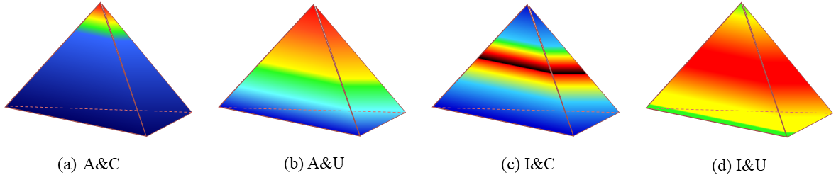
Figure 6: Examples of Probability Simplex. (a) Accurate and Certain (A&C) (b) Accurate and Uncertain (A&U) (c) Inaccurate and Certain (I&C) (d) Inaccurate and Uncertain (I&U).

3. Experimental details of Clinically safety applications.

Finally, we utilize EvidenceCap on two clinical safe applications as a quality indicator and OOD detector for clinicians and patients. In clinical, the OOD sample and the value of data are essential for AI medicine. We employed four real-world clinical datasets for applications of the quality indicator and OOD detector. In the first application, Johns Hopkins OCT (JH-OCT) dataset and Duke OCT dataset with Diabetic Macular Edema (Duke-OCT-DME) are used for the OOD detector. 335 cases of patients on JH-OCT with ground-truth are randomly divided into train dataset, validation dataset and test dataset with nearly 25, 5 and 5 cases, respectively. The 5 cases of test dataset on JH-OCT are used for in-distribution detection. In particular, the 10 cases on the Duke-OCT-DME are used as another test dataset for OOD detection. Every case is uniformly adjusted to $128\times 1024$ voxels during the training and testing.

In the second application, Digital Retinal Images for Vessel Extraction (DRIVE) and the Fundus Image Vessel Segmentation (FIVES) datasets are used for the quality indicator. We first train the EvidenceCap on the DRIVE dataset (20 slices) and then test on the FIVES dataset (600 slices). In the FIVES dataset, each image was evaluated for three qualities: lighting and color distortion, blurring, and low-contrast distortion. We tested on normal images (459 slices with high quality) and images including these three quality ratings (141 slices with low quality) from the FIVES dataset. Every case is uniformly adjusted to $565\times 584$ voxels during the training and testing.

In these applications, the initial learning rate for the dataset are set to be 0.0001. The poly learning strategy is used by decaying each iteration with a power of 0.9. The maximum of the epoch is set to 100. The batch sizes for the layer-segmentation and voxel-segmentation from OCT are set to 8.

4. More visual comparisons

More visual comparisons on ISIC2018, LiTS2017, and BraTS2019 dataset can be seen in the figures 7, 8 and  9. More visual clinical applications on JH-OCT, Duke-OCT-DME, DRIVE and FIVES dataset can be seen in the figures 10.

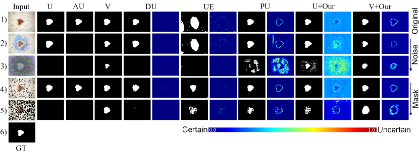
Figure 7: The visual comparison of skin lesion segmentation results with different methods. 1) Original input and its results; (2-3) Input under Gaussian noise ($\sigma^{2}=0.2,0.5$) and its results; (4-5) Input under patch-size mask ($\sigma^{2}=0.1,0.4$) and its results; (6) Ground truth.

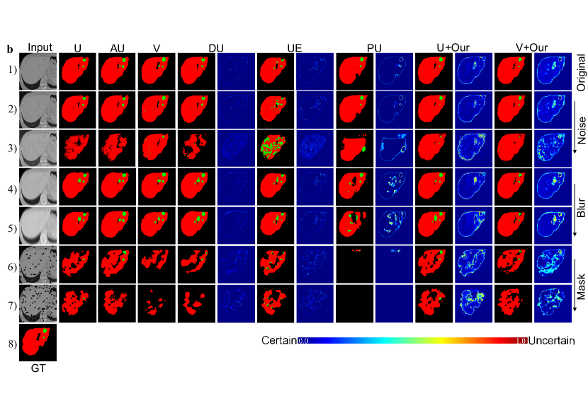
Figure 8: The visual comparison of liver segmentation results with different methods. a) Original input and its results; (b-c) Input under Gaussian noise ($\sigma^{2}=0.2,0.4$) and its results; (d-e) Input under Gaussian blur ($\left\{{\left({{\sigma^{2}},k}\right)}\right\}=\left\{{\left({{\rm{13,10}}}\right),\left({{\rm{15,20}}}\right)}\right\}$) and its results; (f-g) Input under random mask ratio ($\sigma^{2}=0.1,0.3$) and its results; (h) Ground truth.

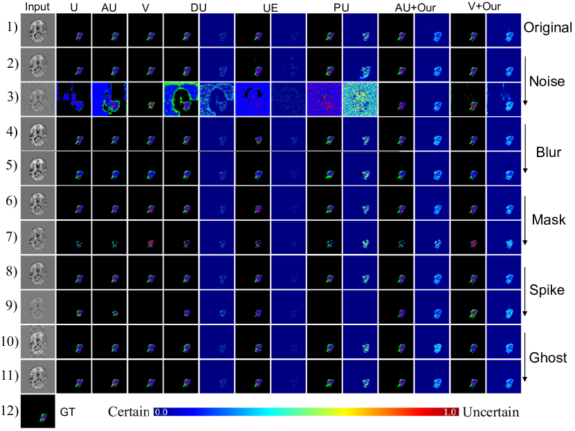
Figure 9: The visual comparison of brain tumor segmentation results with different methods. 1) Original input (T2 as an example); 2)-3) Gaussian noise input under ($\sigma^{2}=1,2$) and its results; 4)-5) Input under Gaussian blur ($\left\{{\left({{\sigma^{2}},k}\right)}\right\}=\left\{{\left({{\rm{3,3}}}\right),\left({{\rm{7,7}}}\right)}\right\}$) and its results. 6)-7) Input under random mask ratio $MR=\left\{{0.1,0.4}\right\}$ and its results; 8) Ground Truth.

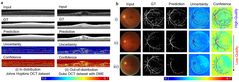
Figure 10: Clinically safety applications for out-of-distribution detector and quality indicator. a. The qualitative difference between in-distribution (JH-OCT dataset without disease) and out-of-distribution data (Duke-OCT-DME). DME: diabetic macular edema. b. Quality difference between image data of different quality, i) Visualization results of high-quality data on the FIVES dataset. ii-iii) Low-quality data visualization results on the FIVES dataset.

References

- [1] F. Isensee, P. F. Jaeger, S. A. Kohl, J. Petersen, and K. H. Maier-Hein, “nnu-net: a self-configuring method for deep learning-based biomedical image segmentation,” Nature methods, vol. 18, no. 2, pp. 203–211, 2021.
- [2] S. P. Primakov, A. Ibrahim, J. E. van Timmeren, G. Wu, S. A. Keek, M. Beuque, R. W. Granzier, E. Lavrova, M. Scrivener, S. Sanduleanu et al., “Automated detection and segmentation of non-small cell lung cancer computed tomography images,” Nature communications, vol. 13, no. 1, pp. 1–12, 2022.
- [3] H. Tang, X. Chen, Y. Liu, Z. Lu, J. You, M. Yang, S. Yao, G. Zhao, Y. Xu, T. Chen et al., “Clinically applicable deep learning framework for organs at risk delineation in ct images,” Nature Machine Intelligence, vol. 1, no. 10, pp. 480–491, 2019.
- [4] R. Zeleznik, B. Foldyna, P. Eslami, J. Weiss, I. Alexander, J. Taron, C. Parmar, R. M. Alvi, D. Banerji, M. Uno et al., “Deep convolutional neural networks to predict cardiovascular risk from computed tomography,” Nature communications, vol. 12, no. 1, pp. 1–9, 2021.
- [5] Z. Cui, Y. Fang, L. Mei, B. Zhang, B. Yu, J. Liu, C. Jiang, Y. Sun, L. Ma, J. Huang et al., “A fully automatic ai system for tooth and alveolar bone segmentation from cone-beam ct images,” Nature communications, vol. 13, no. 1, pp. 1–11, 2022.
- [6] J. Wu, C. Li, M. Gensheimer, S. Padda, F. Kato, H. Shirato, Y. Wei, C.-B. Schönlieb, S. J. Price, D. Jaffray, J. Heymach, J. W. Neal, B. W. Loo, H. Wakelee, M. Diehn, and R. Li, “Radiological tumour classification across imaging modality and histology,” Nature Machine Intelligence, vol. 3, no. 9, pp. 787–798, sep 2021. [Online]. Available: https://www.nature.com/articles/s42256-021-00377-0
- [7] F. Calivà, N. K. Namiri, M. Dubreuil, V. Pedoia, E. Ozhinsky, and S. Majumdar, “Studying osteoarthritis with artificial intelligence applied to magnetic resonance imaging,” Nature Reviews Rheumatology, vol. 18, no. 2, pp. 112–121, feb 2022. [Online]. Available: https://www.nature.com/articles/s41584-021-00719-7
- [8] E. Begoli, T. Bhattacharya, and D. Kusnezov, “The need for uncertainty quantification in machine-assisted medical decision making,” Nature Machine Intelligence, vol. 1, no. 1, pp. 20–23, 2019.
- [9] W. Liang, G. A. Tadesse, D. Ho, F.-F. Li, M. Zaharia, C. Zhang, and J. Zou, “Advances, challenges and opportunities in creating data for trustworthy AI,” Nature Machine Intelligence, aug 2022. [Online]. Available: https://www.nature.com/articles/s42256-022-00516-1
- [10] K. Lee, K. Lee, H. Lee, and J. Shin, “A simple unified framework for detecting out-of-distribution samples and adversarial attacks,” in Advances in neural information processing systems, 2018, pp. 7167–7177.
- [11] J. Long, E. Shelhamer, and T. Darrell, “Fully convolutional networks for semantic segmentation,” in Proceedings of the IEEE conference on computer vision and pattern recognition, 2015, pp. 3431–3440.
- [12] T. Falk, D. Mai, R. Bensch, Ö. Çiçek, A. Abdulkadir, Y. Marrakchi, A. Böhm, J. Deubner, Z. Jäckel, K. Seiwald et al., “U-net: deep learning for cell counting, detection, and morphometry,” Nature methods, vol. 16, no. 1, pp. 67–70, 2019.
- [13] Z. Zhou, M. M. R. Siddiquee, N. Tajbakhsh, and J. Liang, “Unet++: Redesigning skip connections to exploit multiscale features in image segmentation,” IEEE Transactions on Medical Imaging, vol. 39, no. 6, pp. 1856–1867, 2020.
- [14] Ö. Çiçek, A. Abdulkadir, S. S. Lienkamp, T. Brox, and O. Ronneberger, “3d u-net: Learning dense volumetric segmentation from sparse annotation,” in Medical Image Computing and Computer-Assisted Intervention – MICCAI 2016, S. Ourselin, L. Joskowicz, M. R. Sabuncu, G. Unal, and W. Wells, Eds. Cham: Springer International Publishing, 2016, pp. 424–432.
- [15] O. Oktay, J. Schlemper, L. L. Folgoc, M. Lee, M. Heinrich, K. Misawa, K. Mori, S. McDonagh, N. Y. Hammerla, B. Kainz et al., “Attention u-net: Learning where to look for the pancreas,” arXiv:1804.03999, 2018.
- [16] F. Milletari, N. Navab, and S.-A. Ahmadi, “V-net: Fully convolutional neural networks for volumetric medical image segmentation,” in 2016 Fourth International Conference on 3D Vision (3DV), 2016, pp. 565–571.
- [17] A. Vaswani, N. Shazeer, N. Parmar, J. Uszkoreit, L. Jones, A. N. Gomez, Ł. Kaiser, and I. Polosukhin, “Attention is all you need,” Advances in neural information processing systems, vol. 30, 2017.
- [18] A. Dosovitskiy, L. Beyer, A. Kolesnikov, D. Weissenborn, X. Zhai, T. Unterthiner, M. Dehghani, M. Minderer, G. Heigold, S. Gelly et al., “An image is worth 16x16 words: Transformers for image recognition at scale,” arXiv preprint arXiv:2010.11929, 2020.
- [19] J. Chen, Y. Lu, Q. Yu, X. Luo, E. Adeli, Y. Wang, L. Lu, A. L. Yuille, and Y. Zhou, “Transunet: Transformers make strong encoders for medical image segmentation,” arXiv preprint arXiv:2102.04306, 2021.
- [20] Y. Gal and Z. Ghahramani, “Dropout as a bayesian approximation: Representing model uncertainty in deep learning,” in international conference on machine learning. PMLR, 2016, pp. 1050–1059.
- [21] B. Lakshminarayanan, A. Pritzel, and C. Blundell, “Simple and scalable predictive uncertainty estimation using deep ensembles,” Advances in Neural Information Processing Systems, vol. 30, 2017.
- [22] L. Huang, S. Ruan, P. Decazes, and T. Denoeux, “Lymphoma segmentation from 3d pet-ct images using a deep evidential network,” International Journal of Approximate Reasoning, vol. 149, pp. 39–60, 2022.
- [23] J. Van Amersfoort, L. Smith, Y. W. Teh, and Y. Gal, “Uncertainty estimation using a single deep deterministic neural network,” in International Conference on Machine Learning. PMLR, 2020, pp. 9690–9700.
- [24] M. Sensoy, L. Kaplan, and M. Kandemir, “Evidential deep learning to quantify classification uncertainty,” in Proceedings of the 32nd International Conference on Neural Information Processing Systems, 2018, pp. 3183–3193.
- [25] R. McKinley, M. Rebsamen, R. Meier, and R. Wiest, “Triplanar ensemble of 3d-to-2d cnns with label-uncertainty for brain tumor segmentation,” in International MICCAI Brainlesion Workshop. Springer, 2019, pp. 379–387.
- [26] A. Mehrtash, W. M. Wells, C. M. Tempany, P. Abolmaesumi, and T. Kapur, “Confidence calibration and predictive uncertainty estimation for deep medical image segmentation,” IEEE Transactions on Medical Imaging, vol. 39, no. 12, pp. 3868–3878, 2020.
- [27] A. Jungo, R. Meier, E. Ermis, M. Blatti-Moreno, E. Herrmann, R. Wiest, and M. Reyes, “On the effect of inter-observer variability for a reliable estimation of uncertainty of medical image segmentation,” in International Conference on Medical Image Computing and Computer-Assisted Intervention. Springer, 2018, pp. 682–690.
- [28] T. Nair, D. Precup, D. L. Arnold, and T. Arbel, “Exploring uncertainty measures in deep networks for multiple sclerosis lesion detection and segmentation,” Medical image analysis, vol. 59, p. 101557, 2020.
- [29] M. C. Krygier, T. LaBonte, C. Martinez, C. Norris, K. Sharma, L. N. Collins, P. P. Mukherjee, and S. A. Roberts, “Quantifying the unknown impact of segmentation uncertainty on image-based simulations,” Nature communications, vol. 12, no. 1, pp. 1–11, 2021.
- [30] S. Kohl, B. Romera-Paredes, C. Meyer, J. De Fauw, J. R. Ledsam, K. Maier-Hein, S. Eslami, D. Jimenez Rezende, and O. Ronneberger, “A probabilistic u-net for segmentation of ambiguous images,” Advances in Neural Information Processing Systems, vol. 31, 2018.
- [31] J. Mukhoti, J. van Amersfoort, P. H. Torr, and Y. Gal, “Deep deterministic uncertainty for semantic segmentation,” in International Conference on Machine Learning Workshop on Uncertainty and Robustness in Deep Learning, 2021.
- [32] P. Tschandl, C. Rosendahl, and H. Kittler, “The ham10000 dataset, a large collection of multi-source dermatoscopic images of common pigmented skin lesions,” Scientific data, vol. 5, no. 1, pp. 1–9, 2018.
- [33] R. Gu, G. Wang, T. Song, R. Huang, M. Aertsen, J. Deprest, S. Ourselin, T. Vercauteren, and S. Zhang, “Ca-net: Comprehensive attention convolutional neural networks for explainable medical image segmentation,” IEEE Transactions on Medical Imaging, vol. 40, no. 2, pp. 699–711, 2020.
- [34] X. Li, H. Chen, X. Qi, Q. Dou, C.-W. Fu, and P.-A. Heng, “H-denseunet: Hybrid densely connected unet for liver and tumor segmentation from ct volumes,” IEEE Transactions on Medical Imaging, vol. 37, no. 12, pp. 2663–2674, 2018.
- [35] A. Kendall and Y. Gal, “What uncertainties do we need in bayesian deep learning for computer vision?” in NIPS, 2017.
- [36] K. Zou, X. Yuan, X. Shen, M. Wang, and H. Fu, “Tbrats: Trusted brain tumor segmentation,” in International Conference on Medical Image Computing and Computer-Assisted Intervention. Springer, 2022, pp. 503–513.
- [37] L. Daza, J. C. Pérez, and P. Arbeláez, “Towards robust general medical image segmentation,” in International Conference on Medical Image Computing and Computer-Assisted Intervention. Springer, 2021, pp. 3–13.
- [38] W. Wang, C. Chen, M. Ding, H. Yu, S. Zha, and J. Li, “Transbts: Multimodal brain tumor segmentation using transformer,” in Medical Image Computing and Computer Assisted Intervention – MICCAI 2021, 2021, pp. 109–119.
- [39] J. M. J. Valanarasu, V. A. Sindagi, I. Hacihaliloglu, and V. M. Patel, “Kiu-net: Overcomplete convolutional architectures for biomedical image and volumetric segmentation,” IEEE Transactions on Medical Imaging, 2021.
- [40] A. Jøsang, Subjective logic: A Formalism for Reasoning Under Uncertainty. Cham: Springer, 2016.
- [41] Z. Han, C. Zhang, H. Fu, and J. T. Zhou, “Trusted multi-view classification,” in International Conference on Learning Representations, 2021.
- [42] A. P. Dempster, A Generalization of Bayesian Inference. Berlin, Heidelberg: Springer Berlin Heidelberg, 2008, pp. 73–104.
- [43] J. Mukhoti and Y. Gal, “Evaluating bayesian deep learning methods for semantic segmentation,” arXiv preprint arXiv:1811.12709, 2018.
- [44] R. Krishnan and O. Tickoo, “Improving model calibration with accuracy versus uncertainty optimization,” Advances in Neural Information Processing Systems, vol. 33, pp. 18 237–18 248, 2020.
- [45] C. Guo, G. Pleiss, Y. Sun, and K. Q. Weinberger, “On calibration of modern neural networks,” in International conference on machine learning. PMLR, 2017, pp. 1321–1330.
- [46] A. Jungo and M. Reyes, “Assessing reliability and challenges of uncertainty estimations for medical image segmentation,” in International Conference on Medical Image Computing and Computer-Assisted Intervention. Springer, 2019, pp. 48–56.
- [47] K. He, X. Chen, S. Xie, Y. Li, P. Dollár, and R. Girshick, “Masked autoencoders are scalable vision learners,” arXiv preprint arXiv:2111.06377, 2021.
- [48] Y. Gao, M. Zhou, D. Liu, Z. Yan, S. Zhang, and D. N. Metaxas, “A data-scalable transformer for medical image segmentation: Architecture, model efficiency, and benchmark,” 2022.
- [49] B. H. Menze, A. Jakab, S. Bauer, J. Kalpathy-Cramer et al., “The multimodal brain tumor image segmentation benchmark (brats),” IEEE Transactions on Medical Imaging, vol. 34, no. 10, pp. 1993–2024, 2015.
- [50] S. Bakas, M. Reyes, A. Jakab, S. Bauer, M. Rempfler, A. Crimi, R. T. Shinohara, C. Berger, S. M. Ha, M. Rozycki et al., “Identifying the best machine learning algorithms for brain tumor segmentation, progression assessment, and overall survival prediction in the brats challenge,” arXiv preprint arXiv:1811.02629, 2018.