Semidefinite programming on population clustering: a global analysis

Abstract

In this paper, we consider the problem of partitioning a small data sample of size $n$ drawn from a mixture of $2$ sub-gaussian distributions. Our work is motivated by the application of clustering individuals according to their population of origin using markers, when the divergence between the two populations is small. We are interested in the case that individual features are of low average quality $\gamma$, and we want to use as few of them as possible to correctly partition the sample. We consider semidefinite relaxation of an integer quadratic program which is formulated essentially as finding the maximum cut on a graph where edge weights in the cut represent dissimilarity scores between two nodes based on their features. A small simulation result in Blum, Coja-Oghlan, Frieze and Zhou (2007, 2009) shows that even when the sample size $n$ is small, by increasing $p$ so that $np=\Omega(1/\gamma^{2})$, one can classify a mixture of two product populations using the spectral method therein with success rate reaching an “oracle” curve. There the “oracle” was computed assuming that distributions were known, where success rate means the ratio between correctly classified individuals and the sample size $n$. In this work, we show the theoretical underpinning of this observed concentration of measure phenomenon in high dimensions, simultaneously for the semidefinite optimization goal and the spectral method, where the input is based on the gram matrix computed from centered data. We allow a full range of tradeoffs between the sample size and the number of features such that the product of these two is lower bounded by $1/{\gamma^{2}}$ so long as the number of features $p$ is lower bounded by $1/\gamma$.

1 Introduction

We explore a type of classification problem that arises in the context of computational biology. The problem is that we are given a small sample of size $n$, e.g., DNA of $n$ individuals (think of $n$ in the hundreds or thousands), each described by the values of $p$ features or markers, e.g., SNPs (Single Nucleotide Polymorphisms, think of $p$ as an order of magnitude larger than $n$). Our goal is to use these features to classify the individuals according to their population of origin. Features have slightly different probabilities depending on which population the individual belongs to. Denote by $\Delta^{2}$ the $\ell_{2}^{2}$ distance between two population centers (mean vectors), namely, $\mu^{(1)},\mu^{(2)}\in\mathbb{R}^{p}$. We focus on the case where $p>n$, although it is not needed. Note that $\Delta$ measures the Euclidean distance between $\mu^{(1)}$ and $\mu^{(2)}$ and thus represents their separation.

The objective we consider is to minimize the total data size $D=np$ needed to correctly classify the individuals in the sample as a function of the “average quality” $\gamma$ of the features:

$$\gamma:=\Delta^{2}/p,\;\text{ where}\;\;\Delta^{2}:=\sum_{k=1}^{p}(\mu^{(1)}_{k}-\mu^{(2)}_{k})^{2}\;\text{ and }\mu^{(i)}=(\mu^{(i)}_{1},\ldots,\mu^{(i)}_{p})\in\mathbb{R}^{p},i=1,2.$$ (1)

Suppose we are given a data matrix $X\in\mathbb{R}^{n\times p}$ with samples from two populations ${\mathcal{C}}_{1},{\mathcal{C}}_{2}$, such that

$$\forall i\in{\mathcal{C}}_{g},\;\;{\mathbb{E}}(X_{ij})=\mu^{(g)}_{j}\;\;\;g=1,2,\forall j=1,\ldots,p.$$ (2)

Our goal in the present work is to estimate the group membership vector $\bar{x}\in\{-1,1\}^{n}$ such that

$$\bar{x}_{i}=1\;\text{ for }\;i\in{\mathcal{C}}_{1}\;\text{ and }\;\bar{x}_{i}=-1\;\text{ for }\;i\in{\mathcal{C}}_{2},$$ (3)

where the sizes of clusters $\left\lvert{\mathcal{C}}_{j}\right\rvert=:n_{j},\forall j$ may not be the same. Our ultimate goal is to estimate the solution to the discrete optimization problem:

$$\text{maximize}\;\;x^{T}\bar{A}x\quad\text{subject to}\;\;x\in\{-1,1\}^{n}$$ (4)

where $\bar{A}$ is a static reference matrix to be specified. It was previously shown that, in expectation, among all balanced cuts in the complete graph formed among $n$ vertices (sample points), the cut of maximum weight corresponds to the correct partition of the $n$ points according to their distributions in the balanced case ($n_{1}=n_{2}=n/2$). Here the weight of a cut is the sum of weights across all edges in the cut, and the edge weight equals the Hamming distance between the bit vectors of the two endpoints [11, 45]. Under suitable conditions, the statement above also holds with high probability (w.h.p.).

In other words, in the context of population clustering, it has been previously shown one can use a random instance of the integer quadratic program:

$$\text{maximize}\;\;x^{T}Ax\quad\text{ subject to}\quad x\in\{-1,1\}^{n}$$ (5)

to identify the correct partition of nodes according to their population of origin w.h.p., so long as the data size $D$ is sufficiently large and the separation metric is at the order of $\Delta^{2}=\Omega(\log n)$. The analyses focused on the high dimensional setting, where $p\gg n$ [11, 45]. Here $A=(a_{ij})$ is an $n\times n$ symmetric matrix where for $1\leq i,j\leq n$, $a_{ij}=a_{ji}$ denotes the edge weight between nodes $i$ and $j$, computed from the individuals’ bit vectors. This result is structural, rather than algorithmic. The integer quadratic program (4) (or (5)) is NP-hard. In a groundbreaking paper [21], Goemans and Williamson show that one can use semidefinite program (SDP) as relaxation to solve these approximately.

In this paper, we propose a semidefinite relaxation framework, inspired by [22], where we design and analyze computational efficient algorithms to partition data into two groups approximately according to their population of origin. More generally, one may consider semidefinite relaxations for the following sub-gaussian mixture model with $k$ centers (implicitly, with rank-$k$ mean matrix embedded), where

$$X_{i}=\mu^{(\psi_{i})}+{\mathbb{Z}}_{i}$$ (6)

where ${\mathbb{Z}}_{1},\ldots,{\mathbb{Z}}_{n}\in\mathbb{R}^{p}$ are independent, sub-gaussian, mean-zero, random vectors and $\psi_{i}:i\to\{1,\ldots,k\}$ assigns node $i$ to a group ${\mathcal{C}}_{j}$ with the mean $\mu^{(j)}\in\mathbb{R}^{p}$ for some $j\in[k]$. Here we denote by $[k]$ the set of integers $\{1,\ldots,k\}$. Here, each row vector of $X$ is a $p$-dimensional sub-gaussian random vector and we assume rows are independent. We will consider a flexible model of parametrization for ${\mathbb{Z}}_{j},j\in[n]$ in Section 2. In particular, we allow each population to have distinct covariance structures, with diagonal matrices as special cases. The analysis framework for the semidefinite relaxation by Guédon and Vershynin [22] was set in the context of community detection in sparse networks, where $A$ represents the adjacency matrix of a random graph. In other words, they study the semidefinite relaxation of the integer program (5), where an $n\times n$ symmetric random adjacency matrix $A$ (observed) is used to replace the hidden static matrix $\bar{A}$ in the original problem (4) such that ${\mathbb{E}}(A)=\bar{A}$.

The innovative proof strategy of [22] is to apply the Grothendieck’s inequality for the random error $A-\bar{A}$ rather than the original matrix $A$ as considered in the earlier literature. We call this approach the global analysis, following [13]. With proper adjustments, we apply this methodology to our settings and prove the first main Theorem 2.5 regarding the partial recovery of the group memberships based on $n$ sequences of $p$ features following the mean model (2). The important distinction is: here, we replace the random adjacency matrix $A$ arising from stochastic block models as considered in [22] with an instance of symmetric matrix $A$, cf. (9), computed from the centered data matrix which we now elaborate. Let $\mathrm{diag}(A)$ and $\mathrm{offd}(A)$ be the diagonal and the off-diagonal part of matrix $A$ respectively.

Estimators. We propose the following estimators. As in many statistical problems, one simple but crucial step is to first obtain the centered data. Let ${\bf 1}_{n}=[1,\ldots,1]\in\mathbb{R}^{n}$ denote a vector of all $1$s. Let $X$ be a data matrix with row vectors $X_{1},\ldots,X_{n}$ as defined in (2). Denote by

$$Y = X-{\bf 1}_{n}\otimes\widehat{\mu}_{n}=X-P_{1}X,\quad\text{ where}\quad P_{1}=\frac{1}{n}{\bf 1}_{n}{\bf 1}_{n}^{T}\;\;\text{ and }$$ (7)

$$\widehat{\mu}_{n} = \frac{1}{n}\sum_{i}X_{i}\;\text{is the average over $n$ random vectors in $\mathbb{R}^{p}$.}$$ (8)

Loosely speaking, this procedure is called “global centering” in the statistical literature, for example, see [24]. To estimate the group membership vector $\bar{x}\in\{-1,1\}^{n}$, we use the following adjusted $A$:

$$A := YY^{T}-\lambda(E_{n}-I_{n}),\;\;\text{ where}\;\lambda=\frac{2}{n(n-1)}\sum_{i<j}\;\langle{\,Y_{i},Y_{j}\,}\rangle\;,$$ (9)

$$E_{n} := {\bf 1}_{n}{\bf 1}_{n}^{T},\;\text{ and }\;I_{n}\text{ denotes the identity matrix,}$$ (10)

and consider the following semidefinite optimization problem:

SDP: $$\text{maximize}\;\;\;\langle{\,A,Z\,}\rangle\;\;\;\text{ subject to}\quad Z\succeq 0,\;I_{n}\succeq\mathrm{diag}(Z),$$ (11)

where $Z\succeq 0$ indicates that the matrix $Z$ is constrained to be positive semidefinite and $A\succeq B$ means that $A-B\succeq 0$; moreover, the inner product of matrices $\;\langle{\,A,B\,}\rangle\;={\rm tr}(A^{T}B)$. Here and in the sequel, denote by ${\mathcal{M}}^{+}_{G}:=\{Z:Z\succeq 0,I_{n}\succeq\mathrm{diag}(Z)\}$ the set of postive semidefinite matrices whose entries are bounded by 1 in absolute value. More explicitly, the optimization problem SDP (11) is equivalent to:

SDP2: $$\text{maximize}\;\;\;\langle{\,YY^{T}-\lambda E_{n},Z\,}\rangle\;\;\;\text{ subject to}\quad Z\succeq 0,\mathrm{diag}(Z)=I_{n}.$$ (12)

In our setting, centering the data $X$ plays a key role in the statistical analysis and in understanding the roles of sample size lower bounds for partial recovery of the clusters. We mention in passing that our probabilistic analysis in terms of covariance estimation, cf. Theorems 6.3 and 7.2, can be readily applied to the rank-$k$ model (or $k$-means) settings as well. Before we continue, some definitions and notations. Let ${\mathbf{B}}_{2}^{n}$ and $\mathbb{S}^{n-1}$ be the unit Euclidean ball and the unit sphere in $\mathbb{R}^{n}$ respectively.

Definition 1.1.

Recall for a random variable $X$, the $\psi_{2}$-norm of $X$, denoted by $\left\lVert X\right\rVert_{\psi_{2}}$, is $\left\lVert X\right\rVert_{\psi_{2}}=\inf\{t>0\;:\;{\mathbb{E}}\exp(X^{2}/t^{2})\leq 2\}$. A random vector $W\in\mathbb{R}^{m}$ is called sub-gaussian if the one-dimensional marginals $\;\langle{\,W,h\,}\rangle\;$ are sub-gaussian random variables for all $h\in\mathbb{R}^{m}$: (1) $W$ is called isotropic if for every $h\in\mathbb{R}^{m}$, ${\mathbb{E}}\left\lvert\;\langle{\,W,h\,}\rangle\;\right\rvert^{2}=\left\lVert h\right\rVert_{2}^{2}$, where $\left\lVert h\right\rVert_{2}^{2}=\sum_{j=1}^{m}h_{j}^{2}$; (2) $W$ is $\psi_{2}$ with a constant $C_{0}$ if for every $h\in\mathbb{R}^{m}$, $\left\lVert\;\langle{\,W,h\,}\rangle\;\right\rVert_{\psi_{2}}\leq C_{0}\left\lVert h\right\rVert_{2}$. The sub-gaussian norm of $W\in\mathbb{R}^{m}$ is denoted by

$$\left\lVert W\right\rVert_{\psi_{2}}:=\sup_{h\in\mathbb{S}^{m-1}}\left\lVert\;\langle{\,W,h\,}\rangle\;\right\rVert_{\psi_{2}}.$$ (13)

Throughout this paper, we use $Z=(Z_{ij})$ to denote the positive semidefinite matrix in SDP objective functions. We use ${\mathbb{Z}}=(z_{ij})$ to denote the mean-zero random matrix with independent, mean-zero, sub-gaussian row vectors ${\mathbb{Z}}_{1},\ldots,{\mathbb{Z}}_{n}\in\mathbb{R}^{p}$ as considered in (6), where for a constant $C_{0}$ ,

$$\forall j=1,\ldots,n,\;\left\lVert\;\langle{\,{\mathbb{Z}}_{j},x\,}\rangle\;\right\rVert_{\psi_{2}} \leq C_{0}\left\lVert\;\langle{\,{\mathbb{Z}}_{j},x\,}\rangle\;\right\rVert_{L_{2}}\text{ for any }x\in\mathbb{R}^{p}$$ (14)

$$\text{ where }\;\left\lVert\;\langle{\,{\mathbb{Z}}_{j},x\,}\rangle\;\right\rVert^{2}_{L_{2}} := {\mathbb{E}}\;\langle{\,{\mathbb{Z}}_{j},x\,}\rangle\;^{2}=x^{T}{\mathbb{E}}({\mathbb{Z}}_{j}{\mathbb{Z}}_{j}^{T})x=:x^{T}\textsf{Cov}({\mathbb{Z}}_{j})x.$$ (15)

Examples of random vectors with sub-gaussian marginals include the multivariate normal random vectors ${\mathbb{Z}}_{j}\sim N(0,\Sigma)$ with covariance $\Sigma\succ 0$, and vectors with independent Bernoulli random variables, where the mean parameters $p_{j}^{i}:={\mathbb{E}}(X_{ij})$ for all $i\in[n]$ and $j\in[p]$ are assumed to be bounded away from 0 or 1; See for example [11, 9]. For a symmetric matrix $A$, let $\lambda_{\max}(A)$ and $\lambda_{\min}(A)$ be the largest and the smallest eigenvalue of $A$ respectively. The operator norm $\left\lVert A\right\rVert_{2}$ is defined to be $\sqrt{\lambda_{\max}(A^{T}A)}$.

Signal-to-noise ratios and sample lower bounds. Our work is inspired by the two threads of work in combinatorial optimization and in community detection, and particularly by [22] to revisit the max-cut problem (5) and to formulate the SDP (11). Our focus is on the sample size lower bound, similar to the earlier work of the author [11, 45]. Moreover, we adopt the following notion of signal-to-noise ratio when the sub-gaussian random vectors ${\mathbb{Z}}_{i}$ in (6) are isotropic:

$$\text{\bf SNR isotropic: }\quad s^{2}=({\Delta^{2}}/{C_{0}^{2}})\wedge({np\gamma^{2}}/{C_{0}^{4}})$$ (16)

where $C_{0}$ is $\psi_{2}$-constant of the high dimensional vectors ${\mathbb{Z}}_{i}\in\mathbb{R}^{p}$; This notion of SNR appears in [20], which can be properly adjusted when coordinates in ${\mathbb{Z}}_{i}$ are dependent in view of (14) and (15):

$$\text{\bf SNR anisotropic: }\quad s^{2}=\frac{\Delta^{2}}{C_{0}^{2}\max_{j}\left\lVert\textsf{Cov}({\mathbb{Z}}_{j})\right\rVert_{2}}\wedge\frac{np\gamma^{2}}{C_{0}^{4}\max_{j}\left\lVert\textsf{Cov}({\mathbb{Z}}_{j})\right\rVert_{2}^{2}}.$$ (17)

We can rewrite the separation condition that is implicit in Theorem 2.5 as follows:

$$\Delta^{2}=p\gamma\geq C_{0}^{2}\max_{i}\left\lVert\textsf{Cov}({\mathbb{Z}}_{i})\right\rVert_{2}\left(\frac{1}{\xi^{2}}\vee\sqrt{\frac{p}{n\xi^{2}}}\right)\;\text{ for some }\;0<\xi<1/2.$$ (18)

We obtain in Theorem 2.5 misclassification error that is inversely proportional to the square root of the SNR parameter $s^{2}$ as in (16) (resp. (17)) for isotropic ${\mathbb{Z}}_{i}$ (resp. for ${\mathbb{Z}}_{i},i\in[n]$ with covariance structures), assuming that it is lower bounded. In the settings of Theorem 2.5 and Lemma 2.4, we are able to prove that the error decays exponentially with respect to the SNR $s^{2}$ in Theorem 2.7. The implication of such an exponentially decaying error bound is: when $s^{2}=\Omega(\log n)$, perfect recovery of the cluster structure is accomplished. This result is in the same spirit as that in [20]; See also [39, 16, 17] and references therein. Due to its significant length, we defer its proof to another paper. We compare with [16, 17, 20] in the sequel. Also closely related is the work of [9].

In more details, spectral algorithms in [9] partition samples based on the top few eigenvectors of the gram matrix $XX^{T}$, following an idea which goes back at least to [18]. In [9], the two parameters $n,p$ are assumed to be roughly at the same order, hence not allowing a full range of tradeoffs between the two dimensions as considered in the present work; cf (18). The spectral analysis in this paper is based on $YY^{T}$, which will directly improve the results in [9] in the sense that we remove the lower bound on $n$, concerning spectral clustering for $k=2$; cf. Theorem 4.1. Such a lower bound on $n$ was deemed to be unnecessary given the empirical evidence in [9]; See “summary and future direction” in [9].

1.1 Contributions

In summary, we make the following theoretical contributions in this paper: (a) We construct the estimators in (11), which crucially exploit the geometric properties of the two mean vectors, as we show in Section 3; (b) Moreover, we use $YY^{T}$ (and the corresponding $A$ (9)) instead of the gram matrix $XX^{T}$ as considered in [9], as the input to our optimization algorithms, ensuring both computational efficiency and statistical convergence, even in the low SNR case ($s^{2}=o(\log n)$); (c) This approach allows a transparent and unified global and local analysis framework for the semidefinite programming optimization problem (11), as given in Theorems 2.5 and 2.7 respectively; (d) With the new results on concentration of measure bounds on $\left\lVert YY^{T}-{\mathbb{E}}YY^{T}\right\rVert$, we can simultaneously analyze the SDP (11) as well as spectral algorithms based on the leading eigenvector of $YY^{T}$. Here and in the sequel, we use $\left\lVert\cdot\right\rVert$ to indicate either an operator or a cut norm; cf. Definition 3.1.

In Section 4, we make further connections to the existing semidefinite relaxations of the $k$-means clustering problems, which include the baseline spectral algorithm based on the singular value decomposition (SVD) of $YY^{T}$. This allows even faster computation. We analyze a simple spectral algorithm in Theorem 4.1 through the Davis-Kahan Perturbation Theorem, where we obtain error bounds similar to Theorem 2.5. There, we further justify the global centering approach taken in the current paper. We compare numerically the two algorithms, namely, based on SDP and spectral clustering respectively and show they indeed have similar trends as predicted by the signal-to-noise ratio parameter.

1.2 Notations and organizations

Let $e_{1},\ldots,e_{n}$ be the canonical basis of $\mathbb{R}^{n}$. For a set $J\subset\{1,\ldots,n\}$, denote $E_{J}=\operatorname*{span}\{e_{j}:j\in J\}$. Let $P_{1}={\bf 1}_{n}{\bf 1}_{n}^{T}/n$ and $E_{n}=nP_{1}$. Denote by $E_{n\times m}\subset\mathbb{R}^{n\times m}$ a matrix of all ones. For a vector $v\in\mathbb{R}^{n}$, we use $v_{J}$ to denote the subvector $(v_{j})_{j\in J}$. For a vector $x$, $\left\lVert x\right\rVert_{\infty}:=\max_{j}\left\lvert x_{j}\right\rvert$, $\left\lVert x\right\rVert_{1}:=\sum_{j}\left\lvert x_{j}\right\rvert$, and $\left\lVert x\right\rVert_{2}:=\sqrt{\sum_{j}x^{2}_{j}}$; $\mathrm{diag}(x)$ denotes the diagonal matrix whose main diagonal entries are the entries of $x$. For a matrix $B\in\mathbb{R}^{n\times n}$, ${\rm tr}(B)=\sum_{i=1}^{n}B_{ii}$. For a matrix $A=(a_{ij})$ of size $n\times m$, let $\rm{vec}\left\{\,A\,\right\}$ be formed by concatenating columns of matrix $A$ into a long vector of size $nm$; we use $\left\lVert A\right\rVert_{1}=\sum_{i=1}^{n}\sum_{j=1}^{m}|a_{ij}|$ denote the $\ell_{1}$ norm of $\rm{vec}\left\{\,A\,\right\}$, and $\left\lVert A\right\rVert_{F}=(\sum_{i,j}a_{ij}^{2})^{1/2}$ the $\ell_{2}$ norm of $\rm{vec}\left\{\,A\,\right\}$, which is also known as the matrix Frobenius norm. For a matrix $A$, let $\left\lVert A\right\rVert_{\infty}=\max_{i}\sum_{j=1}^{n}|a_{ij}|$ denote the maximum absolute row sum; Let $\left\lVert A\right\rVert_{\max}=\max_{i,j}|a_{ij}|$ denote the component-wise max norm. For two numbers $a,b$, $a\wedge b:=\min(a,b)$, and $a\vee b:=\max(a,b)$. We write $a\asymp b$ if $ca\leq b\leq Ca$ for some positive absolute constants $c,C$ which are independent of $n,p$, and $\gamma$. We write $f=O(h)$ or $f\ll h$ if $\left\lvert f\right\rvert\leq Ch$ for some absolute constant $C<\infty$ and $f=\Omega(h)$ or $f\gg h$ if $h=O(f)$. We write $f=o(h)$ if $f/h\to 0$ as $n\to\infty$, where the parameter $n$ will be the size of the matrix under consideration. In this paper, $C,C_{1},C_{2},C_{4},c,c^{\prime},c_{1}$, etc, denote various absolute positive constants which may change line by line.

The rest of the paper is organized as follows. In Section 2, we present the main theoretical results of the paper. In Section 3, we present the proof outline for Theorem 2.5 on the semidefinite program (11) and concentration of measure bounds on $B$ in Theorem 3.5. In Section 4, we discuss various forms of semidefinite relaxations that have been considered in the literature, and highlight the connections and main differences with the current work. Section 5 gives an outline of the arguments for proving Theorem 3.5, highlighting concentration bounds on $\left\lVert YY^{T}-{\mathbb{E}}YY^{T}\right\rVert$ in Theorems 5.3 and 5.2. In Section 6, we present main ideas in proving Theorem 5.2 with regards to the operator and cut norm using independent design. In Section 7, we discuss correlated design and their concentration of measure bounds concerning Theorem 5.3, one of the most technical results of this paper. Section 8 shows numerical results that validate our theoretical predictions. We conclude in Section 9. We defer all technical proofs to the supplementary material.

2 Theory

We will first construct a matrix $Y$ such that we subtract the sample mean $\widehat{\mu}_{n}\in\mathbb{R}^{p}$ as computed from (8) from each row vector $X_{i}$ of the data matrix. A straight-forward calculation leads to the expression of the reference matrix $R$ in view of (22), and hence ${\mathbb{E}}(Y){\mathbb{E}}(Y)^{T}=R$ for $R$ as in (25).

Definition 2.1.

(The estimators) Let $Y$ be as in (7) and $X$ as in (2). Denote by ${\mathbb{Z}}_{i}=X_{i}-{\mathbb{E}}(X_{i})$ and

$$\widehat{\mu}_{n}-{\mathbb{E}}\widehat{\mu}_{n} := \frac{1}{n}\sum_{i=1}^{n}{\mathbb{Z}}_{i}=\frac{1}{n}\sum_{i=1}^{n}X_{i}-{\mathbb{E}}(X_{i}),$$ (19)

where $\mu_{n}$ is as in (8).

Clearly, by linearity of expectation, ${\mathbb{E}}\widehat{\mu}_{n}=w_{1}\mu^{(1)}+w_{2}\mu^{(2)}$, where $w_{j}={\left\lvert C_{j}\right\rvert}/{n}$ for $j=1,2$. Hence we have for $w_{i}=\left\lvert{\mathcal{C}}_{i}\right\rvert/n,i=1,2$

$${\mathbb{E}}(Y_{i}) := \left\{\begin{array}[]{rl}w_{2}(\mu^{(1)}-\mu^{(2)})&\text{ if }\;i\in{\mathcal{C}}_{1};\\ w_{1}(\mu^{(2)}-\mu^{(1)})&\text{ if }\;i\in{\mathcal{C}}_{2}.\end{array}\right.$$ (22)

Definition 2.2.

(The reference matrix) Denote by $n_{1}=w_{1}n$ and $n_{2}=w_{2}n$. For $Y$ as defined in (7) (cf. Definition 2.1), and $\Delta^{2}=p\gamma$ as in (1), we have

$$R={\mathbb{E}}(Y){\mathbb{E}}(Y)^{T} =: p\gamma\left[\begin{array}[]{cc}w_{2}^{2}E_{n_{1}}&-w_{1}w_{2}E_{n_{1}\times n_{2}}\\ -w_{1}w_{2}E_{n_{2}\times n_{1}}&w_{1}^{2}E_{n_{2}}\end{array}\right].$$ (25)

Definition 2.3.

(Data generative process.) Suppose that random matrix $\mathbb{W}=(w_{jk})\in\mathbb{R}^{n\times m}$ has $W_{1},\ldots,W_{n}\in\mathbb{R}^{m}$ as row vectors, where $W_{j},j\in[n]$ are independent, mean-zero, isotropic sub-gaussian random vectors with independent entries satisfying

$$\forall j\in[n],\quad\textsf{Cov}(W_{j}):={\mathbb{E}}(W_{j}W_{j}^{T})=I_{m},\;\;{\mathbb{E}}[w_{jk}]=0,\forall j,k,\quad\text{and }\;\;\max_{jk}\left\lVert w_{jk}\right\rVert_{\psi_{2}}\leq C_{0}.$$ (26)

Suppose that we have for row vectors of ${\mathbb{Z}}\in\mathbb{R}^{n\times p}$, $\forall j=1,\ldots,n$,

$${\mathbb{Z}}^{T}_{j} = W^{T}_{j}H_{j}^{T}\;\text{ where}\;H_{j}\in\mathbb{R}^{p\times m},\;\;0<\left\lVert H_{j}\right\rVert_{2}<\infty,$$

and $H_{j}$ is allowed to repeat, for example, across rows from the same cluster ${\mathcal{C}}_{i}$ for some $i=1,2$.

Throughout this paper, we assume that $m\geq p$ to simplify our exposition, although this is not necessary. First, Lemma 2.4 characterizes the two-group design matrix variance and covariance structures to be considered in Theorems 2.5 and 2.7. It is understood that when $H_{i}$ is a symmetric square matrix, it can be taken as the unique square root of positive semidefinite covariance matrix, denoted by $\textsf{Cov}({\mathbb{Z}}_{j}):=H_{i}H_{i}^{T}=:\Sigma_{i}\succeq 0$ for all $j\in{\mathcal{C}}_{i}$.

Lemma 2.4.

(two-group sub-gaussian mixture model) Denote by $X$ the two-group design matrix as considered in (2). Let $W_{1},\ldots,W_{n}\in\mathbb{R}^{m}$ be independent, mean-zero, isotropic, sub-gaussian random vectors satisfying (26). Let ${\mathbb{Z}}_{j}=X_{j}-{\mathbb{E}}X_{j}=H_{i}W_{j}$, for all $j\in{\mathcal{C}}_{i}$, where $H_{i}\in\mathbb{R}^{p\times m}$, and $0<\left\lVert H_{i}\right\rVert_{2}<\infty$, for $i\in\{1,2\}$. Then ${\mathbb{Z}}_{1},\ldots,{\mathbb{Z}}_{n}$ are independent sub-gaussian random vectors with $\textsf{Cov}({\mathbb{Z}}_{i})$ satisfying (14) and (15), where

$$\forall j\in{\mathcal{C}}_{i},\quad\textsf{Cov}({\mathbb{Z}}_{j}):={\mathbb{E}}({\mathbb{Z}}_{j}{\mathbb{Z}}_{j}^{T}) = {\mathbb{E}}(H_{i}W_{j}W_{j}^{T}H_{i}^{T})=H_{i}H_{i}^{T}\text{ and }\;V_{i}:=\left\lVert H_{i}\right\rVert_{F}^{2}={\rm tr}(\Sigma_{i}).$$ (27)

2.1 Main results

Throughout this paper, we use $n_{\min}:=nw_{\min}$ and $n_{\max}:=nw_{\max}$ to represent the size of the smallest and the largest clusters respectively. Denote by $w_{\min}:=\min_{j=1,2}w_{j}$, where $w_{j}=n_{j}/n$. We first make the following assumptions (A1) and (A2), assuming random matrix ${\mathbb{Z}}$ has independent sub-gaussian entries, matching the separation (and SNR) condition (29). As a baseline, we state in Theorem 2.5 our first main result under (A1) and (A2). However, the conclusions of Theorem 2.5 hold for the general two-group model so long as (A2) holds, upon adjusting (29).
(A1) Let ${\mathbb{Z}}=X-{\mathbb{E}}X=(z_{ij})$. Let ${\mathbb{Z}}_{i}=X_{i}-{\mathbb{E}}X_{i},i=1,\ldots,n$ be independent, mean-zero, sub-gaussian random vectors with independent coordinates such that for all $i,j$, $\left\lVert z_{ij}\right\rVert_{\psi_{2}}:=\left\lVert X_{ij}-{\mathbb{E}}X_{ij}\right\rVert_{\psi_{2}}\leq C_{0}$.
(A2) The two distributions have variance profile discrepancy bounded in the following sense:

$$\left\lvert V_{1}-V_{2}\right\rvert \leq \frac{1}{3}\xi np\gamma\;\;\text{ for some }\;\;1>2\xi=\Omega(1/n_{\min}),\;\text{ where}\;$$

$$V_{1} = {\mathbb{E}}\;\langle{\,{\mathbb{Z}}_{j},{\mathbb{Z}}_{j}\,}\rangle\;\quad\forall j\in{\mathcal{C}}_{1}\;\;\text{and}\;\;V_{2}={\mathbb{E}}\;\langle{\,{\mathbb{Z}}_{j},{\mathbb{Z}}_{j}\,}\rangle\;\quad\forall j\in{\mathcal{C}}_{2}.$$ (28)

Theorem 2.5.

Let $1>\delta=\Omega(1/n)$. Let ${\mathcal{C}}_{j}\subset[n]$ denote the group membership, with $\left\lvert{\mathcal{C}}_{j}\right\rvert=n_{j}$ and $\sum_{j}n_{j}=n$. Suppose that for $j\in{\mathcal{C}}_{i}$, ${\mathbb{E}}X_{j}=\mu^{(i)}$, where $i=1,2$. Let $\widehat{Z}$ be a solution of the SDP (11). Suppose that (A1) and (A2) hold and for some absolute constants $C,C^{\prime}$,

$$p\gamma=\Delta^{2}\geq\frac{C^{\prime}C_{0}^{2}}{\xi^{2}}\;\;\text{ and }\;pn\geq\frac{CC_{0}^{4}}{\xi^{2}\gamma^{2}},\;\text{ where $\xi$ is the same as in~{}\eqref{eq::Varprofile}}.$$ (29)

Then with probability at least $1-2\exp(-cn)$, we have

$$\left\lVert\widehat{Z}-\bar{x}\bar{x}^{T}\right\rVert_{1}/n^{2} =: \delta\leq{2K_{G}\xi}/{w_{\min}^{2}}\;\;\text{and}\;\;\left\lVert\widehat{Z}-\bar{x}\bar{x}^{T}\right\rVert_{F}^{2}/n^{2}\leq{4K_{G}\xi}/{w_{\min}^{2}},$$ (30)

where $\bar{x}$ is as in (3). The same error bounds (30) also hold for the more general two-group sub-gaussian mixture model as considered in Lemma 2.4, upon adjusting (29), so that (18) holds.

Discussions. We give a proof outline of Theorem 2.5 in Section 3 for completeness. Our proof covers both isotropic and anisotropic cases. See [39, 20] for justifications of (A2). Our analysis shows the surprising result that Theorem 2.5 does not depend on the clusters being balanced, nor does it require identical variance profiles, so long as (A2) holds. Let us also choose a convex subset ${\mathcal{M}}_{\text{opt}}$:

$${\mathcal{M}}_{\text{opt}}=\{Z:Z\succeq 0,\mathrm{diag}(Z)=I_{n}\}\subset{\mathcal{M}}^{+}_{G}.$$ (31)

Our proof follows the sequence of arguments in [22], which were specified for the stochastic block model. However, when adapting to our setting, we crucially use the sub-gaussian concentration of measure bounds as given in Theorems 3.5 and 5.2, as well as verifying a non-trivial global curvature of the excess risk $\;\langle{\,R,Z^{*}-\widehat{Z}\,}\rangle\;$ for the feasible set ${\mathcal{M}}_{\text{opt}}$ at the maximizer $Z^{*}=\mathop{\text{arg\,max}\kern 0.86108pt}_{Z\in{\mathcal{M}}_{\text{opt}}}\;\langle{\,R,Z\,}\rangle\;=\bar{x}\bar{x}^{T}$, cf. Lemma 3.7. In order to control the misclassification error using the global approach, the parameters $(\delta,\xi)$ must satisfy the following: in view of (29) and (30),

$$\xi^{2}\asymp\frac{C_{0}^{2}}{p\gamma}\vee\frac{C_{0}^{4}}{np\gamma^{2}}=1/s^{2}\;\;\text{ and }\;\;\delta\leq\frac{2K_{G}\xi}{w_{\min}^{2}}.$$ (32)

Here the parameter $0<\xi^{2}<1/4$ is understood to be chosen to be inversely proportional to the SNR parameter $s^{2}$, so that with probability at least $1-\exp(-cn)$,

$$\left\lVert YY^{T}-{\mathbb{E}}YY^{T}\right\rVert_{2}\leq C(C_{0}^{2}(\sqrt{pn}\vee n)\vee C_{0}n\sqrt{p\gamma})\asymp\xi np\gamma$$

as we will show in Theorems 5.2 and 5.3.

Clearly, the larger separation $\Delta^{2}$, the larger sample size $n$, and the larger $s^{2}$, the easier it is for (A2) to be satisfied, since by definition and (29),

$$\xi np\gamma\geq n/(\xi)\vee\frac{1}{\xi\gamma}\asymp\sqrt{s^{2}}(n\vee\frac{1}{\gamma})$$

Hence so far, the misclassification error rate $\delta\asymp\xi/w_{\min}^{2}$ is bounded to be inversely proportional to the square root of $s^{2}$. More explicitly, we have Corollary 2.6.

Corollary 2.6.

(Clustering with $o(n)$ misclassified vertices) Let $\widehat{x}$ denote the eigenvector of $\widehat{Z}$ corresponding to the largest eigenvalue, with $\left\lVert\widehat{x}\right\rVert_{2}=\sqrt{n}$. Then in both settings of Theorem 2.5, we have with probability at least $1-2\exp(-cn)$,

$$\min_{\alpha=\pm 1}\left\lVert\alpha\widehat{x}-\bar{x}\right\rVert_{2}^{2}\leq\delta n=\delta\left\lVert\bar{x}\right\rVert_{2}^{2},\;\text{ where}\;\delta\leq{32K_{G}\xi}/{w_{\min}^{2}};$$ (33)

Moreover, the signs of the coefficients of $\widehat{x}$ correctly estimate the partition of the vertices into the two clusters, up to at most $\delta n$ misclassified vertices.

Next, we present in Theorem 2.7 (resp. Corollary 2.8) an error bound (35) (resp. (36)), which decays exponentially in the SNR parameter $s^{2}$ as defined in (17). The settings as considered in Theorem 2.7 include that of Theorem 2.5 as a special case, which we elaborate in Section 2.2. We prove Theorem 2.7 in a concurrent paper. Corollaries 2.6 and 2.8 follow from the Davis-Kahan Theorem, Theorems 2.5 and 2.7 respectively, which we prove in the supplementary Section B.

Theorem 2.7.

Let $W_{1},\ldots,W_{n}\in\mathbb{R}^{m}$ be independent, mean-zero, isotropic, sub-gaussian random vectors satisfying (26). Suppose the conditions in Theorem 2.5 hold, except that instead of (A1), we assume that the noise matrix ${\mathbb{Z}}=X-{\mathbb{E}}(X)$ is generated according to Definition 2.3:

$$\forall j\in{\mathcal{C}}_{i},\quad{\mathbb{Z}}_{j}=H_{i}W_{j}\;\text{ for }\;i\in\{1,2\}\;\;\text{ and }\;H_{i}\in\mathbb{R}^{p\times m},$$

where $0<\left\lVert H_{i}\right\rVert_{2}<\infty$. Suppose that for some absolute constant $C,C_{1}$,

$$p\gamma\geq\frac{CC_{0}^{2}\max_{j}\left\lVert\textsf{Cov}({\mathbb{Z}}_{j})\right\rVert_{2}}{w_{\min}^{4}}\;\;\text{ and }\;\;np\geq\frac{C_{1}C_{0}^{4}\max_{j}\left\lVert\textsf{Cov}({\mathbb{Z}}_{j})\right\rVert_{2}^{2}}{\gamma^{2}w_{\min}^{4}}.$$ (34)

Let $s^{2}$ be as defined in (17). Then with probability at least $1-2\exp(-c_{1}n)-c_{2}/n^{2}$,

$$\left\lVert\widehat{Z}-\bar{x}\bar{x}^{T}\right\rVert_{1}/n^{2}\leq\exp(-c_{0}s^{2}w_{\min}^{4})$$ (35)

for $\widehat{Z}$ as in (11), for some absolute constants $c,c_{0},c_{1}$.

Corollary 2.8.

(Exponential decay in $s^{2}$) Denote by $\theta_{\mathop{\text{SDP}\kern 0.60275pt}}=\angle(\widehat{x},\bar{x})$, the angle between $\widehat{x}$ and $\bar{x}$, where recall $\bar{x}_{j}=1$ if $j\in{\mathcal{C}}_{1}$ and $\bar{x}_{j}=-1$ if $j\in{\mathcal{C}}_{2}$, and $\widehat{x}$ is as in Corollary 2.6. In the settings of Theorem 2.7, with probability at least $1-2\exp(-cn)-2/n^{2}$, for some absolute constants $c,c_{0},c_{1}$,

$$\sin(\theta_{\mathop{\text{SDP}\kern 0.60275pt}}) \leq 2\left\lVert\widehat{Z}-\bar{x}\bar{x}^{T}\right\rVert_{2}/{n}\leq\exp(-c_{1}s^{2}w_{\min}^{4})\;\;\text{ and }$$

$$\min_{\alpha=\pm 1}\left\lVert(\alpha\widehat{x}-\bar{x})/\sqrt{n}\right\rVert_{2} \leq {2^{3/2}\left\lVert\widehat{Z}-\bar{x}\bar{x}^{T}\right\rVert_{2}}/{n}\leq 4\exp(-c_{0}s^{2}w_{\min}^{4}/2)$$ (36)

2.2 Covariance estimation

Remarks on covariance being diagonal. In Theorem 2.5, each noise vector ${\mathbb{Z}}_{j},\forall j\in[n]$ has independent, mean-zero, sub-gaussian coordinates with uniformly bounded $\psi_{2}$ norms. Suppose that we generate two clusters according to Lemma 2.4, with diagonal $H_{1}$ and $H_{2}$ respectively, where

$$H_{j}H^{T}_{j}=\mathrm{diag}(\sigma_{1j}^{2},\ldots,\sigma_{pj}^{2})\quad\forall j\in\{1,2\},$$

Let $\sigma_{\max}:=\max_{i}\left\lVert H_{i}\right\rVert_{2}=(\max_{j,k}{\mathbb{E}}(z_{jk}^{2}))^{1/2}$. Then for each row vector in ${\mathcal{C}}_{i}$, we have

$$\textsf{Cov}({\mathbb{Z}}_{j}) = H_{i}H_{i}^{T}\;\text{ and hence }\;\;V_{i}:={\mathbb{E}}\;\langle{\,{\mathbb{Z}}_{j},{\mathbb{Z}}_{j}\,}\rangle\;={\rm tr}(H_{i}H_{i}^{T})=\sum_{k=1}^{p}\sigma_{ki}^{2}$$

by Lemma 2.4, where $V_{i}$ is the common variance profile for nodes $j\in{\mathcal{C}}_{i}$. Now, we have by independence of coordinates of ${\mathbb{Z}}_{j}$ and by definition of (13)

$$\left\lVert{\mathbb{Z}}_{j}\right\rVert_{\psi_{2}} := \sup_{h\in\mathbb{S}^{p-1}}\left\lVert\;\langle{\,{\mathbb{Z}}_{j},h\,}\rangle\;\right\rVert_{\psi_{2}}\leq C\max_{k\leq p}\left\lVert z_{jk}\right\rVert_{\psi_{2}}\leq CC_{0}(\max_{i}\left\lVert H_{i}\right\rVert_{2})$$

where $\mathbb{S}^{p-1}$ denotes the sphere in $\mathbb{R}^{p}$, and we use (26) and the fact that

$$\max_{k\leq p}\left\lVert z_{jk}\right\rVert_{\psi_{2}}\leq\sigma_{\max}(\max_{j,k}\left\lVert w_{jk}\right\rVert_{\psi_{2}})\leq\sigma_{\max}C_{0}\;\text{ since}\;\left\lVert w_{jk}\right\rVert_{\psi_{2}}\leq C_{0},\forall j,k.$$

Then clearly, $\max_{j}\left\lVert\textsf{Cov}({\mathbb{Z}}_{j})\right\rVert_{2}=\max_{i}\left\lVert H_{i}H_{i}^{T}\right\rVert_{2}=\sigma_{\max}^{2}$ and hence (34) implies that (29) holds; cf.

Remarks on more general covariance. When we allow each population to have distinct covariance structures following Theorem 2.7, we have for some universal constant $C$, and for all $j\in{\mathcal{C}}_{i}$,

$$\left\lVert{\mathbb{Z}}_{j}\right\rVert_{\psi_{2}}:=\sup_{h\in\mathbb{S}^{p-1}}\left\lVert\;\langle{\,{\mathbb{Z}}_{j},h\,}\rangle\;\right\rVert_{\psi_{2}} \leq \left\lVert W_{j}\right\rVert_{\psi_{2}}\left\lVert H_{i}\right\rVert_{2}\leq CC_{0}\max_{i}\left\lVert H_{i}\right\rVert_{2}\;\text{ since }$$ (37)

$$\forall h\in\mathbb{S}^{p-1},\quad\left\lVert\;\langle{\,{\mathbb{Z}}_{j},h\,}\rangle\;\right\rVert_{\psi_{2}} = \left\lVert\;\langle{\,H_{i}W_{j},h\,}\rangle\;\right\rVert_{\psi_{2}}\leq\left\lVert W_{j}\right\rVert_{\psi_{2}}\left\lVert H_{i}^{T}h\right\rVert_{2}$$ (38)

where $\left\lVert W_{j}\right\rVert_{\psi_{2}}\leq CC_{0}$ by definition of (26). Without loss of generality (w.l.o.g.), one may assume that $C_{0}=1$, as one can adjust $H_{i}$ to control the upper bound in (37) through $\left\lVert H_{i}\right\rVert_{2}$. As we will show in Theorems 6.3 and 7.2, with probability at least $1-2\exp(-cn)$, for ${\mathbb{Z}}$ as in Definition 2.3,

$$\frac{1}{p}\left\lVert{\mathbb{Z}}{\mathbb{Z}}^{T}-{\mathbb{E}}{\mathbb{Z}}{\mathbb{Z}}^{T}\right\rVert_{2} \leq C^{\prime}(C_{0}\max_{i}\left\lVert H_{i}\right\rVert_{2})^{2}\left(\sqrt{\frac{n}{p}}\vee\frac{n}{p}\right),$$ (39)

for absolute constants $c,C^{\prime}$. We discuss the concentration of measure bounds on $\left\lVert YY^{T}-{\mathbb{E}}YY^{T}\right\rVert$, using (39) in Sections 5.1 and 7; cf. Lemmas 5.4 and 5.5.

2.3 Related work

In the present work, we use semidefinite relaxation of the graph cut problem (5), which was originally formulated in [11, 45] in the context of population clustering. The biological context for this problem is we are given DNA information from $n$ individuals from $k$ populations of origin and we wish to classify each individual into the correct category. DNA contains a series of markers called SNPs, each of which has two variants (alleles). Given the population of origin of an individual, the genotypes can be reasonably assumed to be generated by drawing alleles independently from the appropriate distribution. In the theoretical computer science literature, earlier work focused on learning from mixture of well-separated Gaussians (component distributions), where one aims to classify each sample according to which component distribution it comes from; See for example [14, 5, 41, 3, 26, 28]. In earlier works [14, 5], the separation requirement depends on the number of dimensions of each distribution; this has recently been reduced to be independent of $p$, the dimensionality of the distribution for certain classes of distributions [3, 27]. While our aim is different from those results, where $n>p$ is almost universal and we focus on cases $p>n$, we do have one common axis for comparison, the $\ell_{2}$-distance between any two centers of the distributions as stated in (40), which is essentially optimal.

Suppose (29) holds so that the $\ell_{2}$-separation and total data size satisfy

$$\Delta^{2}:=p\gamma=\widetilde{\Omega}(1/{(\xi^{2})})\;\text{ and }\;pn=\widetilde{\Omega}({1}/{(\xi^{2}\gamma^{2})}),\;\;\;\text{ where }\;1/n<\xi\leq cw_{\min}^{2}$$ (40)

and the $\widetilde{\Omega}(\cdot)$ symbol only hides $\psi_{2}$-constants for the high dimensional sub-gaussian random vectors ${\mathbb{Z}}_{i}\in\mathbb{R}^{p}$ in (6). Our results show that even when $n$ is small, by increasing $p$ so that the total sample size satisfies (40), we ensure partial recovery of cluster structures using the SDP (11) or the spectral algorithm as described in Theorem 4.1. Previously, such results were only known to exist for balanced max-cut algorithms [45, 11], where $\widetilde{\Omega}(\cdot)$ symbol in (40) may also hide logarithmic factors. Results in [45, 11] were among the first such results towards understanding rigorously and intuitively why their proposed algorithms and previous methods [34, 37] work with low sample settings when $p\gg n$ and $np$ satisfies (40). These earlier results still need the SNR to be at the order of $s^{2}=O(\log n)$; Moreover these results were structural as no polynomial time algorithms were given for finding the max-cut.

The main contribution of the present work is: we use the proposed SDP (11) and the related spectral algorithms to find the partition, and prove quantitively tighter bounds than those in [45, 11] by removing these logarithmic factors. Recently, this barrier has also been broken down by the sequence of work [39, 16, 20], which we elaborate in Section 4, cf. Variation 3. For example, [16, 17] have also established exponentially decaying error bounds with respect to an appropriately defined SNR, which focuses on balanced clusters and requires an extra $\sqrt{\log n}$ factor in (41) in the second component:

$$\text{In~{}\cite[cite]{[\@@bibref{Number}{FC18}{}{}]}, cf. eq.(8): }\quad\Delta^{2}=p\gamma = \Omega\left(1+\sqrt{\frac{p\log n}{n}}\right)\quad\text{or }$$ (41)

$$\text{In~{}\cite[cite]{[\@@bibref{Number}{FC21}{}{}]}, cf. eq.(13): }\quad\Delta^{2}=p\gamma = \Omega\left((1\vee\frac{p}{n})+\sqrt{\frac{p\log n}{n}}\right)$$ (42)

As a result, in (42), a lower bound on the sample size is imposed: $n\geq 1/\gamma$ in case $p>n$, and moreover, the size of the matrix $np\geq\log n/\gamma^{2}$, similar to the bounds in [9]; cf. Theorem 1.2 therein. We refer to [11, 9] for references to earlier results on spectral clustering and graph partitioning. We also refer to [26, 38, 22, 1, 7, 12, 8, 20, 29, 17, 30, 2, 32] and references therein for related work on the Stochastic Block Models (SBM), mixture of (sub)Gaussians and clustering in more general metric spaces. Our proof technique may be of independent interests, since centering the data matrix so that each column has empirical mean 0 is an idea broadly deployed in statistical data analysis.

3 The (oracle) estimators and the global analysis

Exposition in this subsection follows that of [22], which we include for self-containment. First we state Grothendieck’s inequality following [22]. The concept of cut-norm plays a major role in the work of Frieze and Kannan [19] on efficient approximation algorithms for dense graph and matrix problems. The cut norm is also crucial for the arguments in [22] to go through.

Definition 3.1.

(Matrix cut norm) For a matrix $A=(a_{ij})$, we denote by $\left\lVert(a_{ij})\right\rVert_{\infty\to 1}$ its $\ell_{\infty}\to\ell_{1}$ norm, which is

$$\left\lVert(a_{ij})\right\rVert_{\infty\to 1} = \max_{\left\lVert s\right\rVert_{\infty}\leq 1}\left\lVert As\right\rVert_{1}=\max_{s,t\in\left\{-1,1\right\}^{n}}\;\langle{\,A,st^{T}\,}\rangle\;$$

This norm is equivalent to the matrix cut norm defined as: for $A\in\mathbb{R}^{m\times n}$,

$$\left\lVert A\right\rVert_{\square} = \max_{I\subset[m],J\subset[n]}\left\lvert\sum_{i\in I}\sum_{j\in J}a_{i,j}\right\rvert$$

and hence

$$\left\lVert A\right\rVert_{\infty\to 1} = \max_{x,y\in\{-1,1\}^{n}}\sum_{i=1}^{n}\sum_{j=1}^{n}a_{ij}x_{i}y_{i}\leq\left\lVert x\right\rVert_{2}\left\lVert y\right\rVert_{2}\left\lVert A\right\rVert_{2}\leq n\left\lVert A\right\rVert_{2}$$

Theorem 3.2.

(Grothendieck’s inequality) Consider an $n\times n$ matrix of real numbers $B=(b_{ij})$. Assume that, for any numbers $s_{i},t_{j}\in\{-1,1\}$, we have

$$\left\lvert\sum_{i,j}b_{ij}s_{i}t_{j}\right\rvert=\left\lvert\;\langle{\,B,st^{T}\,}\rangle\;\right\rvert\leq 1$$ (43)

Then for all vectors $S_{i},V_{i}\in B_{2}^{n}$, we have $\left\lvert\sum_{i,j}b_{ij}\;\langle{\,S_{i},V_{j}\,}\rangle\;\right\rvert=\left\lvert\;\langle{\,B,SV^{T}\,}\rangle\;\right\rvert\leq K_{G}$, where $K_{G}$ is an absolute constant referred to as the Grothendieck’s constant:

$$K_{G}\leq\frac{\pi}{2\ln(1+\sqrt{2})}\leq 1.783.$$ (44)

Here $B_{2}^{n}=\{x\in\mathbb{R}^{n}:\left\lVert x\right\rVert_{2}\leq 1\}$ denotes the unit ball for Euclidean norm. Consider the following two sets of matrices:

$${\mathcal{M}}_{1}:=\left\{st^{T}\;:\;s,t\in\{-1,1\}^{n}\right\},\quad{\mathcal{M}}_{G}:=\left\{SV^{T}:\;\text{ all rows}\;S_{i},V_{j}\in B_{2}^{n}\right\}.$$

Clearly, ${\mathcal{M}}_{1}\subset{\mathcal{M}}_{G}$. As a consequence, Grothendieck’s inequality can be stated as follows:

$$\forall B\in\mathbb{R}^{n\times n}\;\;\max_{Z\in{\mathcal{M}}_{G}}\left\lvert\;\langle{\,B,Z\,}\rangle\;\right\rvert\leq K_{G}\max_{Z\in{\mathcal{M}}_{1}}\left\lvert\;\langle{\,B,Z\,}\rangle\;\right\rvert.$$ (45)

Clearly, the RHS (45) can be related to the cut norm in Definition 3.1:

$$\max_{Z\in{\mathcal{M}}_{1}}\left\lvert\;\langle{\,B,Z\,}\rangle\;\right\rvert=\max_{s,t\in\{-1,1\}^{n}}\;\langle{\,B,st^{T}\,}\rangle\;=\left\lVert B\right\rVert_{\infty\to 1}$$ (46)

To keep the discussion sufficiently general, following [22], we first let ${\mathcal{M}}_{\text{opt}}$ be any subset of the Grothendieck’s set ${\mathcal{M}}_{G}^{+}$ defined in (47):

$${\mathcal{M}}_{G}^{+}:=\left\{Z:Z\succeq 0,\mathrm{diag}(Z)\preceq I_{n}\right\}\subset{\mathcal{M}}_{G}\subset[-1,1]^{n\times n}.$$ (47)

Lemma 3.3 elaborates on the relationship between $\widehat{Z}$ for any given $B$ (random or deterministic), and $Z^{*}$ with respect to the objective function using $R$, as defined in (48). Let

$$\widehat{Z}:=\mathop{\text{arg\,max}\kern 0.86108pt}_{Z\in{\mathcal{M}}_{\text{opt}}}\;\langle{\,B,Z\,}\rangle\;\quad\text{and}\quad Z^{*}:=\mathop{\text{arg\,max}\kern 0.86108pt}_{Z\in{\mathcal{M}}_{\text{opt}}}\;\langle{\,R,Z\,}\rangle\;$$ (48)

Lemma 3.3.

(Lemma 3.3 [22]) Let ${\mathcal{M}}_{\text{opt}}$ be any subset of $M_{G}^{+}\subset[-1,1]^{n\times n}$ as defined in (47). Then for $\widehat{Z}$ and $Z^{*}$ as defined in (48),

$$\;\langle{\,R,Z^{*}\,}\rangle\;-2K_{G}\left\lVert B-R\right\rVert_{\infty\to 1}\leq\;\langle{\,R,\widehat{Z}\,}\rangle\;\leq\;\langle{\,R,Z^{*}\,}\rangle\;$$ (49)

where the Grothendieck’s constant $K_{G}$ is the same as defined in (44). Then

$$0\leq\;\langle{\,R,Z^{*}-\widehat{Z}\,}\rangle\; \leq 2K_{G}\left\lVert B-R\right\rVert_{\infty\to 1}\;\;\text{moreover, we have}$$ (50)

$$\sup_{Z\in{\mathcal{M}}_{\text{opt}}}\left\lvert\;\langle{\,B-R,Z-Z^{*}\,}\rangle\;\right\rvert \leq 2K_{G}\left\lVert B-R\right\rVert_{\infty\to 1}$$ (51)

Lemma 3.3 shows that $\widehat{Z}$ as defined in (48) for the original problem for a given $B$ provides an almost optimal solution to the reference problem if the original matrix $B$ and the reference matrix $R$ are close. Lemma 3.3 motivates the consideration of the oracle $B$ as defined in (52) in Section 3 and $\widehat{Z}$ as in (48). Lemma 3.3 appears as Lemma 3.3 in [22]. We include the proof in the supplementary Section C for self-containment.

3.1 The oracle estimators

The overall goal of convex relaxation is to: (a) estimate the solution of the discrete optimization problem (4) with an appropriately chosen reference matrix $R$ such that solving the integer quadratic problem (4) (with $R$ replacing $\bar{A}$) will recover the cluster exactly; (b) Moreover, the convex set ${\mathcal{M}}^{+}_{G}$ (resp. ${\mathcal{M}}_{\text{opt}}$) is chosen such that the semidefinite relaxation of the static problem (4) is tight. This means that when we replace $A$ (resp. $A^{\prime}$) with $R={\mathbb{E}}(Y){\mathbb{E}}(Y)^{T}$ in SDP (11) (resp. SDP2 (12)), we obtain a solution $Z^{*}=\bar{x}\bar{x}^{T}$, which can then be used to recover the clusters exactly; cf. Lemma 3.6.

Note that unlike the settings of [22], ${\mathbb{E}}A\not=R$, resulting in a bias; However, a remedy is to transform (11) into an equivalent Oracle SDP formulation to bridge the gap between $YY^{T}$ and the reference matrix $R$ which we now define: recall ${\mathcal{M}}_{\text{opt}}=\left\{Z:Z\succeq 0,\mathrm{diag}(Z)=I_{n}\right\}\subset{\mathcal{M}}^{+}_{G}$,

$${\bf OracleSDP:} \text{maximize}\;\;\;\langle{\,B,Z\,}\rangle\;\quad\text{ subject to}\quad Z\in{\mathcal{M}}_{\text{opt}}\;\text{where}$$ (52)

$$B := A-{\mathbb{E}}\tau I_{n}\;\;\;\text{ where }\;\;\tau=\frac{1}{n}\sum_{i=1}^{n}\;\langle{\,Y_{i},Y_{i}\,}\rangle\;$$ (53)

and $A$ is as in (11).

Moreover, on ${\mathcal{M}}_{\text{opt}}$, the adjustment term ${\mathbb{E}}\tau I_{n}$ plays no role in optimization, since the extra trace term $\propto\;\langle{\,I_{n},Z\,}\rangle\;={\rm tr}(Z)$ is a constant function of $Z$ across the feasible set ${\mathcal{M}}_{\text{opt}}$. However, the diagonal term ${\mathbb{E}}\tau I_{n}$ is added in (53) so that the bias $\left\lVert{\mathbb{E}}B-R\right\rVert$ is small. To conclude, the optimization goal (11) is equivalent to (52) in view of Proposition 3.4; cf (55). In words, optimizing the original SDP (11) over the larger constraint set ${\mathcal{M}}^{+}_{G}$ is equivalent to maximizing $\;\langle{\,B,Z\,}\rangle\;$ over $Z\in{\mathcal{M}}_{\text{opt}}$ as shown in (55), where we replace the symmetric matrix $A$ with $B$.

Proposition 3.4.

The optimal solutions $\widehat{Z}$ as in (11) must have their diagonals set to $I_{n}$. Thus, the set of optimal solutions $\widehat{Z}$ in (11) coincide with those on the convex subset ${\mathcal{M}}_{\text{opt}}$ as in (31),

$$\mathop{\text{arg\,max}\kern 0.86108pt}_{Z\in{\mathcal{M}}^{+}_{G}}\;\langle{\,A,Z\,}\rangle\; = \mathop{\text{arg\,max}\kern 0.86108pt}_{Z\in{\mathcal{M}}_{\text{opt}}}\;\langle{\,A,Z\,}\rangle\;$$ (54)

$$= \mathop{\text{arg\,max}\kern 0.86108pt}_{Z\in{\mathcal{M}}_{\text{opt}}}(\;\langle{\,A,Z\,}\rangle\;-{\mathbb{E}}\tau\;\langle{\,I_{n},Z\,}\rangle\;).$$ (55)

We prove Proposition 3.4 in the supplementary Section C.2. We emphasize that our algorithm solves the SDP (11) rather than the oracle SDP (52). However, formulating the oracle SDP (52) helps us with the global analysis, in controlling $\left\lVert{\mathbb{E}}B-R\right\rVert$, as we now show in Theorem 3.5.

Theorem 3.5.

($R$ is the leading term) Suppose the conditions in Theorem 2.5 hold. Then with probability at least $1-2\exp(-cn)$, we have

$$\left\lVert B-R\right\rVert_{2} \leq \xi np\gamma\;\text{ and }\;\left\lVert B-R\right\rVert_{\infty\to 1}\leq\xi n^{2}p\gamma$$

Discussions. Notice that $B$ is not attainable, since we do not know ${\mathbb{E}}\tau$; however, this is irrelevant, since in the proposed algorithm (11), we are able to readily compute $A$ using the centered data (or their gram matrix). Theorem 3.5 is useful in proving Theorem 2.5 in view of Lemma 3.3; A proof sketch for Theorem 3.5 appears in Section 5 and the complete proof appears in the supplementary Section D. The effectiveness of the SDP procedure (11) crucially depends on controlling the bias term $\left\lVert{\mathbb{E}}B-R\right\rVert_{\infty\to 1}$ as well as the concentration of measure bounds on $\left\lVert B-{\mathbb{E}}B\right\rVert_{\infty\to 1}$, which in turn depend on Lemma 5.1, Theorems 5.2 and 5.3 respectively. As we will show in the proof of Theorem 3.5, the bias term

$${\mathbb{E}}B-R = {\mathbb{E}}YY^{T}-{\mathbb{E}}(Y){\mathbb{E}}(Y)^{T}-{\mathbb{E}}\lambda(E_{n}-I_{n})-{\mathbb{E}}\tau I_{n}$$

is substantially smaller than ${\mathbb{E}}A-R$ in the operator and cut norm, under assumption (A2). Moreover, the concentration of measure bounds on $\left\lVert YY^{T}-{\mathbb{E}}YY^{T}\right\rVert$ imply that, up to a constant factor, the same bounds also hold for $\left\lVert B-{\mathbb{E}}B\right\rVert$. Controlling both leads to the conclusion in Theorem 3.5.

In Theorem 4.1, we prove convergence results on bounding the angle and $\ell_{2}$ distance between the leading eigenvectors of $R$ and $B$ (resp. $YY^{T}$) respectively. Indeed, computing the operator and cut norm for $B-R$ is one of the key technical steps in the current work, unifying Theorems 4.1 and 2.5.

3.2 Proof of Theorem 2.5

Lemma 3.6 shows that the outer product of group membership vector, namely, $Z^{*}$ will maximize $\;\langle{\,R,Z\,}\rangle\;$ among all $Z\in[-1,1]^{n\times n}$, and naturally among all $Z\in{\mathcal{M}}_{\text{opt}}$. The final result we need is to verify a non-trivial global curvature of the excess risk $\;\langle{\,R,Z^{*}-\widehat{Z}\,}\rangle\;$ for the feasible set ${\mathcal{M}}_{\text{opt}}$ at the maximizer $Z^{*}$, which is given in Lemma 3.7. We then combine Lemmas 3.3 and 3.7, and Theorem 3.5 to obtain the final error bound for $\lVert\widehat{Z}-Z^{*}\rVert$ in the $\ell_{1}$ or Frobenius norm. Recall $\left\lVert A\right\rVert_{1}=\sum_{i,j}\left\lvert a_{ij}\right\rvert$.

Lemma 3.6.

(Optimizer of the reference objective function) Let $R$ be as defined in Definition 2.2. Let ${\mathcal{M}}_{\text{opt}}\subseteq{\mathcal{M}}_{G}^{+}\subset[-1,1]^{n\times n}$ be as defined in (31). Then

$$Z^{*}=\mathop{\text{arg\,max}\kern 0.86108pt}_{Z\in{\mathcal{M}}_{\text{opt}}}\;\langle{\,R,Z\,}\rangle\;=\left[\begin{array}[]{cc}E_{n_{1}}&-E_{n_{1}\times n_{2}}\\ -E_{n_{2}\times n_{1}}&E_{n_{2}}\end{array}\right]=\bar{x}\bar{x}^{T}$$ (58)

The proof of Lemma 3.7 follows from ideas in Lemma 6.2 [22] and is deferred to the supplementary Section C.4. As a result, we can apply the Grothendieck’s inequality for the random error $B-R$ (cf. Lemma 3.3) to obtain an upper bound on $\;\langle{\,R,Z^{*}-\widehat{Z}\,}\rangle\;$ uniformly for all $\widehat{Z}\in{\mathcal{M}}_{\text{opt}}$, where $Z^{*}$ is as defined in (58). Putting things together, we can prove Theorem 2.5.

Lemma 3.7.

Let $R$ be as defined in Definition 2.2 and $Z^{*}$ be as in (58). For every $Z\in{\mathcal{M}}_{\text{opt}}$,

$$\;\langle{\,R,Z^{*}-Z\,}\rangle\;\geq p\gamma w_{\min}^{2}\left\lVert Z-Z^{*}\right\rVert_{1}.$$ (59)

Proof of Theorem 2.5.   We will first conclude from Theorem 3.5 and Lemma 3.3 that the maximizer of the actual objective function $\widehat{Z}=\mathop{\text{arg\,max}\kern 0.86108pt}_{Z\in{\mathcal{M}}_{\text{opt}}}\;\langle{\,B,Z\,}\rangle\;,$ must be close to $Z^{*}$ as in (58) in terms of the $\ell_{1}$ distance. Under the conditions of Lemmas 3.3 and 3.7,

$$\left\lVert\widehat{Z}-Z^{*}\right\rVert_{1}/n^{2} \leq \frac{\;\langle{\,R,Z^{*}-\widehat{Z}\,}\rangle\;}{n^{2}p\gamma w_{\min}^{2}}\leq\frac{2K_{G}\left\lVert B-R\right\rVert_{\infty\to 1}}{n^{2}p\gamma w_{\min}^{2}}\leq\frac{2K_{G}\xi}{w_{\min}^{2}}=:\delta$$

where by Theorem 3.5, $\left\lVert B-R\right\rVert_{\infty\to 1}\leq\xi n^{2}p\gamma$. Thus

$$\left\lVert Z^{*}-\widehat{Z}\right\rVert_{F}^{2} \leq \left\lVert Z^{*}-\widehat{Z}\right\rVert_{\max}\left\lVert Z^{*}-\widehat{Z}\right\rVert_{1}\leq 2\delta$$

where all entries of $\widehat{Z},Z^{*}$ belong to $[-1,1]$ and hence $\left\lVert Z^{*}-\widehat{Z}\right\rVert_{\max}\leq 2$.  $\;\;\scriptstyle\Box$

4 Semidefinite programming relaxation for clustering

Denote by $X\in\mathbb{R}^{n\times p}$ the data matrix with row vectors $X_{i}$ as in (60). The $k$-means criterion of a partition ${\mathcal{C}}=\{C_{1},\ldots,{\mathcal{C}}_{k}\}$ of sample points $\{1,\ldots,n\}$ is based on the total sum-of-squared Euclidean distances from each point $X_{i}\in\mathbb{R}^{p}$ to its assigned cluster centroid ${\bf c}_{j}$, namely,

$$f(X,{\mathcal{C}},k):=\sum_{j=1}^{k}\sum_{i\in{\mathcal{C}}_{j}}\left\lVert X_{i}-{\bf c}_{j}\right\rVert_{2}^{2}\;\text{ where}\;\;{\bf c}_{j}:=\frac{1}{\left\lvert{\mathcal{C}}_{j}\right\rvert}\sum_{\ell\in{\mathcal{C}}_{j}}X_{\ell}\in\mathbb{R}^{p}$$ (60)

Getting a global solution to (60) through an integer programming formulation as in [36, 35], is NP-hard and it is NP-hard for $k=2$ [15, 4]. Various semidefinite relaxations of the objective function have been considered in different contexts. We refer to [44, 35, 6, 25, 29, 31, 39, 16, 20, 17] and references therein for a more complete picture. Let $\Psi_{n}$ denote the linear space of real $n$ by $n$ symmetric matrices.

Representation of the partition. The work by [44, 36, 35] show that minimizing the $k$-means objective $f(X,{\mathcal{C}},k)$ is equivalent to solving the following maximization problem:

$$\text{maximize}\;\;\;\langle{\,\widehat{S}_{n},Z\,}\rangle\;\quad\text{ s.t. }Z\in{\mathcal{P}}_{k}$$ (61)

where $\widehat{S}_{n}=XX^{T}$ and the constraint set ${\mathcal{P}}_{k}$ is defined as in (62):

$$\mathcal{P}_{k}=\{B\in\Psi_{n}:B\geq 0,B^{2}=B,B{\bf 1}_{n}={\bf 1}_{n},{\rm tr}(B)=k\}$$ (62)

where $B\geq 0$ means that all elements of $B$ are nonnegative. Hence matrices in ${\mathcal{P}}_{k}$ are block diagonal, symmetric, nonnegative projection matrices with ${\bf 1}_{n}$ as an eigenvector. The following matrix set $\Phi_{n,k}$ is a compact convex subset of $\Psi_{n}$, for any $k\in[n]$:

$$\Phi_{n,k}=\left\{Z\in\Psi_{n}:I_{n}\succeq Z\succeq 0,{\rm tr}(Z)=k\right\}$$ (63)

Variation 1. Peng and Wei [35] first replace the requirement that $Z^{2}=Z$, namely, $Z$ is a projection matrix, with the relaxed condition that all eigenvalues of $Z$ must stay in $[0,1]$: $I_{n}\succeq Z\succeq 0$. Now consider the following semidefinite relaxation of  (61),

$$\text{maximize}\quad\;\langle{\,\widehat{S}_{n},Z\,}\rangle\;\text{ s.t.}\;Z\in{\mathcal{M}}_{k}\;\text{ where }\;{\mathcal{M}}_{k}=\{Z\in\Phi_{n,k}:Z\geq 0,Z{\bf 1}_{n}={\bf 1}_{n}\}$$ (64)

The key differences between this and the SDP (11) are: (a) In the convex set ${\mathcal{M}}_{\text{opt}}$ (31), we do not enforce that all entries are nonnegative, namely, $Z_{ij}\geq 0,\forall i,j$; This allows faster computation; (b) In order to derive concentration of measure bounds that are sufficiently tight, we make a natural, yet important data processing step in the current work, where we center the data according to their column means following Definition 2.1 before computing $A$ as in (9); (c) Given this centering step, we do not need to enforce $Z{\bf 1}_{n}={\bf 1}_{n}$. See Variation 2 for details.

Variation 2. To speed up computation, one can drop the nonnegative constraint on elements of $Z$ in (64) [44, 35]. The following semidefinite relaxation is also considered in [35]:

$$\text{maximize}\quad\;\langle{\,\widehat{S}_{n},Z\,}\rangle\; \text{ s.t. }\;Z{\bf 1}_{n}={\bf 1}_{n},Z\in\Phi_{n,k}\;\;\text{ for }\;\Phi_{n,k}\text{ as in}~{}\eqref{eq::tracek}.$$ (65)

Moreover, Peng and Wei [35] show that the set of feasible solutions to (65) have immediate connections to the SVD of $YY^{T}$, via the following reduction step, closely related to our proposal. When $Z$ is a feasible solution to (65), ${\bf 1}_{n}/\sqrt{n}$ is the unit-norm leading eigenvector of $Z$ and one can define

$$Z_{1} := Z-\frac{1}{n}{\bf 1}_{n}{\bf 1}_{n}^{T}\;\;\text{ and hence }\;\;Z_{1}:=(I-P_{1})Z=(I-P_{1})Z(I-P_{1}).$$ (66)

Then ${\rm tr}(Z_{1})={\rm tr}(Z)-1=k-1$ and $Z_{1}\in\Phi_{n,k-1}$. Hence (65) is reduced to

$$\text{maximize}\quad\;\langle{\,YY^{T},Z_{1}\,}\rangle\;\quad\text{ s.t. }I_{n}\succeq Z_{1}\succeq 0,{\rm tr}(Z_{1})=k-1$$ (67)

since $YY^{T}=(I-P_{1})\widehat{S}_{n}(I-P_{1})$. Let $\lambda_{1}\geq\ldots\geq\lambda_{n-1}$ be the largest $(n-1)$ eigenvalues of $YY^{T}$ in descending order. The optimal solution to (67) can be achieved if and only if $\;\langle{\,YY^{T},Z_{1}\,}\rangle\;=\sum_{i=1}^{k-1}\lambda_{i}$; see for example [33]. Then the algorithm for solving (67) and correspondingly (65) is given as follows [35]:
(a) Use singular value decomposition method to compute the first $k-1$ largest eigenvalues of $YY^{T}$, and their corresponding eigenvectors $v_{1},\ldots,v_{k-1}$; (b) Set

$$Z_{1}=\sum_{j=1}^{k-1}v_{j}v_{j}^{T};\;\;\text{and return}\;\;Z=\frac{1}{n}{\bf 1}_{n}{\bf 1}_{n}^{T}+Z_{1}\;\text{ as a solution to \eqref{eq::relax17}}.$$

Now for $k=2$, we have $Z_{1}=v_{1}v_{1}^{T}$. In Theorem 4.1, we show convergence for the angle as well as the $\ell_{2}$ distance between the two vectors $v_{1}$ and $\bar{v}_{1}$, where $v_{1}$ and $\bar{v}_{1}$ are the leading eigenvectors of $YY^{T}$ and the reference matrix $R$ respectively. Theorem 4.1 demonstrates another excellent application of our estimation procedure and concentration of measure bounds, namely, Theorem 3.5.

Theorem 4.1.

(SVD: imbalanced case) Denote by $v_{1}$ the leading unit-norm eigenvector of $YY^{T}$, which also coincides with that of $A$ (9) and $B$ (53). Let $\bar{v}_{1}$ be the leading unit-norm eigenvector of $R$ as in (25):

$$\bar{v}_{1}=[w_{2}{\bf 1}_{n_{1}},-w_{1}{\bf 1}_{n_{2}}]/\sqrt{w_{2}w_{1}n}=[\sqrt{w_{2}/w_{1}}{\bf 1}_{n_{1}},-\sqrt{w_{1}/w_{2}}{\bf 1}_{n_{2}}]/{\sqrt{n}},$$ (68)

where $\;\langle{\,\bar{v}_{1},{\bf 1}_{n}\,}\rangle\;=0$. Then under the conditions in Theorem 3.5, we have with probability at least $1-2\exp(-cn)$, for some absolute constants $c,c_{0},c_{1},c_{2}$,

$$\sin(\theta_{1}) := \sin(\angle({v}_{1},\bar{v}_{1}))\leq\frac{2\left\lVert B-R\right\rVert_{2}}{w_{1}w_{2}np\gamma}\leq\frac{2\xi}{w_{1}w_{2}}$$ (69)

$$\min_{\alpha=\pm 1}\left\lVert\alpha v_{1}-\bar{v}_{1}\right\rVert_{2}^{2} \leq \delta^{\prime},\text{ where}\;\;\delta^{\prime}={8\xi^{2}}/{(w_{1}^{2}w_{2}^{2})}\leq c_{2}\xi^{2}/w_{\min}^{2};$$ (70)

where $\theta_{1}=\angle({v}_{1},\bar{v}_{1})$ denotes the angle between the two vectors $v_{1}$ and $\bar{v}_{1}$.

Corollary 4.2.

(Clustering with $o(n/s^{2})$ misclassified vertices) Suppose that $w_{1},w_{2}\in(0,1)$ are bounded away from $0,1$. Under the conditions in Theorem 4.1, we have with probability at least $1-2\exp(-cn)$, for some absolute constants $c$, the signs of the coefficients of $v_{1}$ correctly estimate the partition of the vertices into two clusters, up to at most $O(\xi^{2}n)$ misclassified vertices.

Discussions. We prove Theorem 4.1 and its corollary in the supplementary Section E. The signs of the coefficients of $v_{1}$ correctly estimate the partition of the vertices, up to at most $\delta^{\prime}n\asymp\xi^{2}n$ misclassified vertices, where recall $\xi^{2}\asymp 1/s^{2}$ (32). Hence the misclassification error is bounded to be inversely proportional to the SNR parameter $s^{2}$; cf. (32). This should be compared with (33), where we show in Theorem 2.5 that we have up to at most $\delta n\asymp\xi n$ misclassified vertices, which is improved to $O(n\exp(-c_{0}s^{2}w_{\min}^{4}))$ in Theorem 2.7. Moreover, one can sort the values of $v_{1}$ and find the nearly optimal partition according to the $k$-means criterion; See Section 8 for Algorithm 2 and numerical examples.

Variation 3. The main issue with the $k$-means relaxation is that the solutions tend to put sample points into groups of the same sizes, and moreover, the diagonal matrix $\Gamma$ can cause a bias, where

$$\Gamma=({\mathbb{E}}[\;\langle{\,{\mathbb{Z}}_{i},{\mathbb{Z}}_{j}\,}\rangle\;])_{i,j}=\mathrm{diag}([{\rm tr}(\textsf{Cov}({\mathbb{Z}}_{1})),\ldots,{\rm tr}(\textsf{Cov}({\mathbb{Z}}_{n}))]),$$

especially when $V_{1},V_{2}$ differ from each other; See the supplementary Section H for bias analysis. In [39, 20, 10], they propose a preliminary estimator of $\Gamma$, denoted by $\widehat{\Gamma}$, and consider

$$\widehat{Z}\in\arg\max_{Z\in{\mathcal{M}}_{k}}\;\langle{\,XX^{T}-\widehat{\Gamma},Z\,}\rangle\;\;\;\text{ where}\;{\mathcal{M}}_{k}\;\text{ is as in~{}\eqref{eq::relax16} }$$ (71)

instead of the original Peng-Wei SDP relaxation (64). Although our general results in Theorem 2.7 coincide with that of [20] for $k=2$, we emphasize that we prove these bounds for the SDP (11), which is motivated by the graph partition problem (5), while they establish such bounds for the semidefinite relaxation based on the $k$-means criterion (60) directly, following [35]. There, cf. (64), and (71), the matrix $Z$ is not only constrained to be positive semidefinite but also with non-negative entries. As mentioned, the advantage of dropping the nonnegative constraints on elements of $Z$ in (11) is to speed up the computation.

Hence another main advantage of our SDP and spectral formulation is that we do not need to have a separate estimator for ${\rm tr}(\Sigma_{j})$, where $\Sigma_{j},j=1,2$ denote the covariance matrices of sub-gaussian random vectors ${\mathbb{Z}}_{j},j\in[n]$, so long as (A2) holds. When it does not, one may consider adopting similar ideas. We emphasize that part of our probabilistic bounds, namely, Theorems 6.3 and 7.2, already work for the general $k$-means clustering problem.

5 Outline of the arguments for proving Theorem 3.5

We emphasize that results in this section apply to both settings under consideration: design matrix with independent entries or with independent anisotropic sub-gaussian rows. This allows us to prove Theorem 3.5 for both cases. Let $Y$ be as in Definition 2.1. By definition of (9) and (53),

$$A-{\mathbb{E}}A=B-{\mathbb{E}}B := YY^{T}-{\mathbb{E}}YY^{T}-(\lambda-{\mathbb{E}}\lambda)(E_{n}-I_{n})$$ (72)

$$\text{ hence}\;\left\lVert B-R\right\rVert_{\infty\to 1} = \left\lVert B-{\mathbb{E}}B+{\mathbb{E}}B-R\right\rVert_{\infty\to 1}$$ (73)

$$\leq \left\lVert B-{\mathbb{E}}B\right\rVert_{\infty\to 1}+\left\lVert{\mathbb{E}}B-R\right\rVert_{\infty\to 1}$$

We have by the triangle inequality, (72), (73) and the supplementary Lemma D.1, for

$$\left\lVert B-R\right\rVert_{2} \leq 2\left\lVert\Psi\right\rVert_{2}+\left\lVert{\mathbb{E}}B-R\right\rVert_{2}\;\text{ where }\;\Psi:=YY^{T}-{\mathbb{E}}(YY^{T}),$$ (74)

$$\text{ and }\;\;\left\lVert B-R\right\rVert_{\infty\to 1} \leq \left\lVert\Psi\right\rVert_{\infty\to 1}+n\left\lVert\Psi\right\rVert_{2}+\left\lVert{\mathbb{E}}B-R\right\rVert_{\infty\to 1}$$

Lemma 5.1 states that the bias ${\mathbb{E}}B-R$ is substantially reduced for $B$ as in (53), thanks to the adjustment term ${\mathbb{E}}\tau I_{n}$, and even more so when clusters have similar variance profiles in the sense that (28) is bounded. Theorem 3.5 follows immediately from Lemma 5.1 and Theorem 5.2 (resp. 5.3), where we bound $\left\lVert YY^{T}-{\mathbb{E}}(YY^{T})\right\rVert$ for design matrix with independent entries (resp. with independent anisotropic sub-gaussian rows). All results except for Theorems 5.2 and 5.3 are stated as deterministic bounds. Let $c_{7},c_{8},C_{2},C_{3},\ldots$ be some absolute constants. All constants such as $1/6,2/3,\ldots$ are arbitrarily chosen.

Lemma 5.1.

Suppose (A2) holds. Suppose that $\xi\geq\frac{1}{2n}(4\vee\frac{1}{w_{\min}})$ and $n\geq 4$. Then we have

$$\left\lVert{\mathbb{E}}B-R\right\rVert_{2} \leq \frac{2}{3}\xi np\gamma\;\text{ and }\;\left\lVert{\mathbb{E}}B-R\right\rVert_{\infty\to 1}\leq\frac{2}{3}\xi n^{2}p\gamma$$

Finally, when $V_{1}=V_{2}$, we have $\left\lVert{\mathbb{E}}B-R\right\rVert_{\infty\to 1}\leq n\left\lVert{\mathbb{E}}B-R\right\rVert_{2}\leq pn\gamma/3$.

Theorem 5.2.

(Design with independent entries) In the initial settings as specified in Theorem 2.5, suppose that $(A1)$, $(A2)$ and (29) hold with $\max_{j,k}\left\lVert z_{jk}\right\rVert_{\psi_{2}}:=\left\lVert X_{jk}-{\mathbb{E}}X_{jk}\right\rVert_{\psi_{2}}\leq C_{0}$. Then, with probability at least $1-2\exp(-c_{7}n)$,

$$\left\lVert YY^{T}-{\mathbb{E}}(YY^{T})\right\rVert_{2} \leq C_{2}C_{0}^{2}(\sqrt{pn}\vee n)+C_{3}C_{0}n\sqrt{p\gamma}\leq\frac{1}{6}\xi np\gamma$$

Theorem 5.3.

(Anisotropic design matrix.) Let $Y$ be as in Definition 2.1. Suppose all conditions in Theorem 2.5 and Lemma 2.4 hold. Suppose (18) holds. Then with probability at least $1-2\exp(-c_{8}n)$,

$$\left\lVert YY^{T}-{\mathbb{E}}(YY^{T})\right\rVert_{2} \leq \frac{1}{12}\xi np\gamma+C_{4}(C_{0}\max_{i}\left\lVert H_{i}\right\rVert_{2})^{2}(\sqrt{pn}\vee n)\leq\frac{1}{6}\xi np\gamma.$$

where $C_{0}$ is the same as in (18) and (37).

We prove Lemma 5.1 in the supplementary Section H.2, where balanced cases are shown to be slightly more tightly bounded; cf Lemma H.7 therein. We prove Theorems 5.2 and 5.3 in the supplementary Section F.1 and Section 7 respectively. It is understood that for both theorems, we also obtain $\left\lVert YY^{T}-{\mathbb{E}}(YY^{T})\right\rVert_{\infty\to 1}$ to be within a factor of $O(n)\lVert YY^{T}-{\mathbb{E}}(YY^{T})\rVert_{2}$. We prove Theorem 3.5 in the supplementary Section D.

5.1 Reduction

In this section, we present a unified framework for bounding $\left\lVert YY^{T}-{\mathbb{E}}YY^{T}\right\rVert_{2}$. First,

$$YY^{T}-{\mathbb{E}}(YY^{T})=YY^{T}-{\mathbb{E}}(Y){\mathbb{E}}(Y)^{T}+{\mathbb{E}}(Y){\mathbb{E}}(Y)^{T}-{\mathbb{E}}(YY^{T})$$ (75)

$$= {\mathbb{E}}(Y)(Y-{\mathbb{E}}(Y))^{T}+(Y-{\mathbb{E}}(Y))({\mathbb{E}}(Y))^{T}+\widehat{\Sigma}_{Y}-\Sigma_{Y}$$

where $\widehat{\Sigma}_{Y}=(Y-{\mathbb{E}}(Y))(Y-{\mathbb{E}}(Y))^{T}$ and

$$\widehat{\Sigma}_{Y}-\Sigma_{Y} = (Y-{\mathbb{E}}(Y))(Y-{\mathbb{E}}(Y))^{T}+{\mathbb{E}}(Y){\mathbb{E}}(Y)^{T}-{\mathbb{E}}(YY^{T}),$$

from which we obtain from the well known relationship on covariance matrix

$$\Sigma_{Y}:={\mathbb{E}}\left((Y-{\mathbb{E}}(Y))(Y-{\mathbb{E}}(Y))^{T}\right)={\mathbb{E}}(YY^{T})-{\mathbb{E}}(Y){\mathbb{E}}(Y)^{T}.$$

We now state in Lemma 5.4 a reduction principle for bounding the first component in (75): To control

$$\left\lVert M_{Y}\right\rVert=\left\lVert{\mathbb{E}}(Y)(Y-{\mathbb{E}}(Y))^{T}+(Y-{\mathbb{E}}(Y))({\mathbb{E}}(Y))^{T}\right\rVert,$$

we need to bound the projection of each mean-zero random vector ${\mathbb{Z}}_{j},\forall j\in[n]$, along the direction of $v:=\mu^{(1)}-\mu^{(2)}$. In other words, a particular direction for which we compute the one-dimensional marginals, is the direction between $\mu^{(1)}$ and $\mu^{(2)}$.

Lemma 5.4.

(Reduction: a deterministic comparison lemma) Let ${\mathbb{Z}}_{j},j\in[n]$ be row vectors of $X-{\mathbb{E}}X$ and $\widehat{\mu}_{n}$ be as defined in (8). For $x_{i}\in\{-1,1\}$,

$$\sum_{i=1}^{n}x_{i}\;\langle{\,Y_{i}-{\mathbb{E}}Y_{i},\mu^{(1)}-\mu^{(2)}\,}\rangle\; \leq \frac{2(n-1)}{n}\sum_{i=1}^{n}\left\lvert\;\langle{\,{\mathbb{Z}}_{i},\mu^{(1)}-\mu^{(2)}\,}\rangle\;\right\rvert$$ (76)

Then we have for $M_{Y}:={\mathbb{E}}(Y)(Y-{\mathbb{E}}(Y))^{T}+(Y-{\mathbb{E}}(Y))({\mathbb{E}}(Y))^{T}$,

$$\left\lVert M_{Y}\right\rVert_{\infty\to 1} \leq 8w_{1}w_{2}(n-1)\sum_{i=1}^{n}\left\lvert\;\langle{\,{\mathbb{Z}}_{i},\mu^{(1)}-\mu^{(2)}\,}\rangle\;\right\rvert\;\text{ and}\;$$

$$\left\lVert M_{Y}\right\rVert_{2} \leq 4\sqrt{n}\sqrt{w_{1}w_{2}}\sup_{q\in S^{n-1}}\left\lvert\sum_{i}q_{i}\;\langle{\,{\mathbb{Z}}_{i},\mu^{(1)}-\mu^{(2)}\,}\rangle\;\right\rvert$$

Upon obtaining (22), Lemma 5.4 is deterministic and does not depend on covariance structure of ${\mathbb{Z}}$. On the other hand, controlling the second component in (75) amounts to the problem of covariance estimation given the mean matrix ${\mathbb{E}}(Y)$; Lemma 5.5 is again deterministic, where we show that controlling the operator (and cut) norm of $\widehat{\Sigma}_{Y}-\Sigma_{Y}$ is reduced to controlling that for ${\mathbb{Z}}{\mathbb{Z}}^{T}-{\mathbb{E}}({\mathbb{Z}}{\mathbb{Z}}^{T})$. We prove Lemmas 5.4 and 5.5 in the supplementary Sections F.2 and F.3 respectively.

Lemma 5.5.

Suppose that $Y$ and $Z$ are matrices as defined in Definition 2.1. The following holds:

$$\widehat{\Sigma}_{Y}-\Sigma_{Y}=(I-P_{1})({\mathbb{Z}}{\mathbb{Z}}^{T}-{\mathbb{E}}({\mathbb{Z}}{\mathbb{Z}}^{T}))(I-P_{1})$$

cf. Proposition F.1 in the supplementary material. Then $\left\lVert\widehat{\Sigma}_{Y}-\Sigma_{Y}\right\rVert_{2}\leq\left\lVert{\mathbb{Z}}{\mathbb{Z}}^{T}-{\mathbb{E}}({\mathbb{Z}}{\mathbb{Z}}^{T})\right\rVert_{2}$.

6 Proof outline of Theorem 5.2

We provide a proof outline for Theorem 5.2 in this section. We will bound these two components (75) in Lemma 6.1 and Theorem 6.3 respectively. Lemma 6.1 follows from Lemma 5.4 and the sub-gaussian concentration of measure bounds in Lemma 6.2. We will only state the operator norm bound in Theorem 6.3, with the understanding that cut norm of a matrix is within $O(n)$ factor of the operator norm on the same matrix. We defer the proof of Theorems 5.2 and 6.3 to the supplementary Sections F.1 and G.3 respectively. The proof for Lemmas 6.1 and 6.2 appear in the supplementary Section G. Let $c,c^{\prime},c_{1},c_{5},C_{3},C_{4},\ldots$ be absolute constants.

Lemma 6.1.

(Projection: probabilistic view) Suppose conditions in Theorem 5.2 hold. Then we have with probability at least $1-2\exp(-cn)$,

$$\left\lVert{\mathbb{E}}(Y)(Y-{\mathbb{E}}(Y))^{T}+(Y-{\mathbb{E}}(Y))({\mathbb{E}}(Y))^{T}\right\rVert_{2} \leq 2C_{3}C_{0}n\sqrt{p\gamma}\text{ and}\;$$

$$\left\lVert{\mathbb{E}}(Y)(Y-{\mathbb{E}}(Y))^{T}+(Y-{\mathbb{E}}(Y))({\mathbb{E}}(Y))^{T}\right\rVert_{\infty\to 1} \leq C_{4}C_{0}n(n-1)\sqrt{p\gamma}$$

Lemma 6.2 follows from the sub-gaussian tail bound, since the one-dimensional marginals of ${\mathbb{Z}}_{j},\forall j\in[n]$ are sub-gaussian with bounded $\psi_{2}$ norms. Denote by

$$\mu:=\frac{\mu^{(1)}-\mu^{(2)}}{\left\lVert\mu^{(1)}-\mu^{(2)}\right\rVert_{2}}=\frac{\mu^{(1)}-\mu^{(2)}}{\sqrt{p\gamma}}\in\mathbb{S}^{p-1}$$ (77)

Lemma 6.2.

(Projection for sub-gaussian random vectors) In the settings of Theorem 5.2, suppose (A1) holds and $C_{0}=\max_{i,j}\left\lVert z_{ij}\right\rVert_{\psi_{2}}$. Then for any $t>0$, and any $u=(u_{1},\ldots,u_{n})\in\{-1,1\}^{n}$

$$\mathbb{P}\left(\sum_{i=1}^{n}u_{i}\;\langle{\,{\mathbb{Z}}_{i},\mu\,}\rangle\;\geq t\right) \leq 2\exp\left(-{ct^{2}}/{(C_{0}^{2}n)}\right);$$ (78)

$$\text{and for any }\;q\in\mathbb{S}^{n-1},\mathbb{P}\left(\sum_{i=1}^{n}\;\langle{\,q_{i}{\mathbb{Z}}_{i},\mu\,}\rangle\;\geq t\right) \leq 2\exp\left(-{c^{\prime}t^{2}}/{C_{0}^{2}}\right)$$ (79)

Theorem 6.3.

In the settings of Theorem 5.2, we have with probability at least $1-2\exp(-c_{6}n)$,

$$\left\lVert\widehat{\Sigma}_{Y}-{\mathbb{E}}\widehat{\Sigma}_{Y}\right\rVert_{2} = \left\lVert{\mathbb{E}}({\mathbb{Z}}{\mathbb{Z}}^{T})-{\mathbb{E}}({\mathbb{Z}}{\mathbb{Z}}^{T})\right\rVert_{2}\leq C_{2}C_{0}^{2}(\sqrt{pn}+n)\leq\frac{1}{12}\xi np\gamma.$$

7 Proof outline for Theorem 5.3

We provide an outline for Theorem 5.3 in this section. First, we state Lemma 7.1, where we extend Lemma 6.1 to the anisotropic cases. The anisotropic version of Lemma 6.2 is presented in the supplementary Lemma I.1. The model under consideration in Theorem 7.2 is understood to be a special case of Theorem 7.3. Theorem 5.3 follows from Theorem 7.2 and Lemma 7.1 immediately, and the probability statements hold upon adjusting the constants. We defer all proofs to the supplementary Section I. Let $c,c^{\prime},C_{2},C_{3},C_{4},\ldots$ be absolute constants.

Lemma 7.1.

(Projection: probabilistic view) Let $\mu$ be as in (77) and $M_{Y}$ be as in Lemma 5.4. Suppose all conditions in Theorem 5.3 hold. Then with probability at least $1-2\exp(-c^{\prime}n)$, we have

$$\left\lVert M_{Y}\right\rVert_{\infty\to 1} \leq C_{4}(C_{0}\max_{i}\left\lVert R_{i}\mu\right\rVert_{2})n(n-1)\sqrt{p\gamma}\leq\frac{1}{12}\xi n(n-1)p\gamma$$

$$\left\lVert M_{Y}\right\rVert_{2} \leq 2C_{3}(C_{0}\max_{i}\left\lVert R_{i}\mu\right\rVert_{2})n\sqrt{p\gamma}\leq\frac{1}{12}\xi np\gamma$$

Theorem 7.2.

In the settings of Theorem 5.3, we have with probability at least $1-2\exp(-c_{6}n)$,

$$\left\lVert\widehat{\Sigma}_{Y}-{\mathbb{E}}\widehat{\Sigma}_{Y}\right\rVert_{2} \leq \left\lVert{\mathbb{Z}}{\mathbb{Z}}^{T}-{\mathbb{E}}{\mathbb{Z}}{\mathbb{Z}}^{T}\right\rVert_{2}\leq C_{2}(C_{0}\max_{i}\left\lVert H_{i}\right\rVert_{2})^{2}(\sqrt{np}\vee n).$$ (80)

Theorem 7.3.

(Hanson-Wright inequality for anisotropic sub-gaussian vectors.) Let $H_{1},\ldots,H_{n}$ be deterministic $p\times m$ matrices, where we assume that $m\geq p$. Let ${\mathbb{Z}}^{T}_{1},\ldots,{\mathbb{Z}}^{T}_{n}\in\mathbb{R}^{p}$ be row vectors of ${\mathbb{Z}}$. We generate ${\mathbb{Z}}$ according to Definition 2.3.

Then we have for $t>0$, for any $A=(a_{ij})\in\mathbb{R}^{n\times n}$,

$$\mathbb{P}\left(\left\lvert\sum_{i=1}^{n}\sum_{j\not=i}^{n}\;\langle{\,{\mathbb{Z}}_{i},{\mathbb{Z}}_{j}\,}\rangle\;a_{ij}\right\rvert>t\right)$$ (81)

$$\leq 2\exp\left(-c\min\left(\frac{t^{2}}{(C_{0}\max_{i}\left\lVert H_{i}\right\rVert_{2})^{4}p\left\lVert A\right\rVert_{F}^{2}},\frac{t}{(C_{0}\max_{i}\left\lVert H_{i}\right\rVert_{2})^{2}\left\lVert A\right\rVert_{2}}\right)\right)$$

where $\max_{i}\left\lVert{\mathbb{Z}}_{i}\right\rVert_{\psi_{2}}\leq CC_{0}\max_{i}\left\lVert H_{i}\right\rVert_{2}$ in the sense of (37).

Remarks on covariance estimation. Essentially, (80) matches the optimal bounds on covariance estimation, where the mean-zero random matrix consists of independent columns ${\mathbb{Z}}^{j},j=1,\ldots,p$ that are isotropic, sub-gaussian random vectors in $\mathbb{R}^{n}$, or columns which can be transformed to be isotropic through a common covariance matrix. See, for example, Theorems 4.6.1 and 4.7.1 [42]. The difference between (80) and such known results are: (a) we do not assume that columns are independent; (b) we do not require anisotropic row vectors to share identical covariance matrices. More generally, we allow the (sample by sample) covariance matrix $\Sigma_{X}:={\mathbb{E}}{\mathbb{Z}}{\mathbb{Z}}^{T}=\mathrm{diag}([{\rm tr}(H_{1}H_{1}^{T}),\ldots,{\rm tr}(H_{n}H_{n}^{T})])$, through Definition 2.3; and hence we are estimating a diagonal matrix with $p$ dependent features, where we assume that ${\mathbb{E}}(X)$ is given. We state the operator norm bound in Theorem 7.2, where it is understood that (80) holds under the general covariance model as considered in Definition 2.3 and Theorem 7.3. We prove Theorem 7.3 in the supplementary Section I.4. The proof might be of independent interests. Such generalization is useful since we may consider the more general $k$-component mixture problems, as elaborated in Section 4. See also Exercise 6.2.7 [42] for a related result.

8 Experiments

In this section, we use simulation to illustrate the effectiveness and convergence properties of the two estimators. We use a similar setup as the one used in  [9]. We generate data that is a mixture of two populations. Data matrix $X\in\{0,1\}^{n\times p}$ consists of independent Bernoulli random variables, where the mean parameters ${\mathbb{E}}(X_{ij}):=q_{\psi(i)}^{j}$ for all $i\in[n]$ and $j\in[p]$, where $\psi(i)\in\{1,2\}$ assigns nodes $i$ to a group ${\mathcal{C}}_{1}$ or ${\mathcal{C}}_{2}$ for each $i\in[n]$. Let $\left|{\mathcal{C}}_{1}\right|=w_{1}n$ and $\left|{\mathcal{C}}_{2}\right|=w_{2}n$. We conduct experiments for both balanced ($w_{1}=w_{2}$) and imbalanced cases. The entrywise expected values are chosen as follows: for half of the $p$ features, the mean parameters $q_{1}^{j}>q_{2}^{j}$, and for the other half, $q_{1}^{j}<q_{2}^{j}$ such that $\forall j$, $q_{1}^{j},q_{2}^{j}\in\{\frac{1+\alpha}{2}+\frac{\epsilon}{2},\frac{1-\alpha}{2}+\frac{\epsilon}{2}\}$. We set $\epsilon=0.1\alpha$ and $\alpha=0.04$. Hence $\gamma=\alpha^{2}=0.0016$, $\frac{1}{\gamma^{2}}=390,625$, and $\frac{1}{\gamma}=625$. We implement Algorithm 1: the SDP as described in (11), and classify according to signs of $\widehat{x}$ as prescribed by Corollary 2.6; and Algorithm 2: the Peng-Wei spectral method following [35].
Algorithm 2: Spectral method for $k$-means clustering (Peng-Wei) [35]: Input: Centered data matrix $Y\in\mathbb{R}^{n\times p}$, $k=2$ Output: A group assignment vector $P$ Step 1. Use SVD to obtain the leading eigenvector $v_{1}$ of $YY^{T}$ and let $v:=v_{1}$; Step 2. Let $S$ be the vector of sorted values of $v$ in descending order. For each index $j$ in $[n]$, compute the two means ${\bf c}_{1}$, ${\bf c}_{2}$, one for each of the two groups, namely, ${\mathcal{C}}_{1}=S_{L}:=\{S_{1},\ldots,S_{j}\}$ and ${\mathcal{C}}_{2}=S_{R}:=\{S_{j+1},\ldots,S_{n}\}$ to the left (inclusive) and the right of this index; Step 3. Compute the total sum-of-squared Euclidean distances from each point within a particular group to the respective mean, according to (60); Let $t$ be the index that gives the minimum total distance, and its corresponding value be $S_{t}$; Step 4. Set $P_{i}=1$ if $v_{i}\geq S_{t}$, and $P_{i}=-1$ if $v_{i}<S_{t}$.

Success rate and misclassification rate. For each experiment, we run 100 trials; and for each trial, we first generate a data matrix $X_{n\times p}$ according to the mixture of two Bernoulli distributions with parameters described above, and then feed $Y$ (7) to the two estimators for classification. We measure success rate and misclassification rate based on $P$, the output assignment vector. Success rate is computed as the number of correctly classified individuals divided by the sample size $n$. Hence misclassification rate is $1-$ success rate. Each data point corresponds to the average of 100 trials. Fig. 1 shows the average success rates (over $100$ trials) as $n$ increases for different values of $p$ for the balanced case.

We observe that SDP has higher average success rate for each setting of $(n,p)$ when $np\gamma^{2}>1.5$, despite the exhaustive search in Algorithm 2; For $np\gamma^{2}<1.5$, the rates are closer. We also see from the plot that when $p<1/\gamma=625$, for example, when $p=500$, the success rate remains flat across $n$. Note that a success rate of $50\%$ is equivalent to a total failure. In contrast, when $n$ is smaller than $1/\gamma$, as we increase $p$, we can always classify with a high success rate. In general, $np\gamma^{2}>1$ is indeed necessary to obtain a success rate larger than $60\%$, when $p\geq 1/{\gamma}$. When $n<625$, $np\gamma^{2}$ plays the role of the SNR, since $np\gamma^{2}<p\gamma$; This remains the case throughout our experiments.

Angle and $\ell_{2}$ convergence. Here we take a closer look at the trends of $\widehat{x}$ and $\widehat{Z}$, the solution to SDP (11) as $n$ increases, and of $v_{1}$, the leading eigenvector of $YY^{T}$. In the second experiment, we set $p\in\{20000,50000,80000\}$, and increase $n$. In the left column of Fig. 2, which is for the imbalanced case of $w_{1}=0.7$, we plot $\theta_{\mathop{\text{SDP}\kern 0.60275pt}}:=\angle(\widehat{x},\bar{x})$ between $\widehat{x}$ and its reference vector $\bar{x}$ as defined in Theorem 2.5 and Corollary 2.6.

For Algorithm 2, $\theta_{1}:=\angle(v_{1},\bar{v}_{1})$ between $v_{1}$ and its reference $\bar{v}_{1}$, where $\bar{v}_{1}$ is as defined in Theorem 4.1. In this case, the angle $\angle(\bar{v}_{1},\bar{x})$ between the two reference vectors is about 22 degrees (blue horizontal dashed line). We observe that as $n$ increases, for both algorithms, the angles $\theta_{\mathop{\text{SDP}\kern 0.60275pt}}$ and $\theta_{1}$ decrease, but $\theta_{\mathop{\text{SDP}\kern 0.60275pt}}$ drops much faster and decreases to $0$ when $n>200$ for $p=80,000$. We also show the angle $\phi=\angle(\widehat{x},v_{1})$ between the two leading eigenvectors $\widehat{x}$ and $v_{1}$, which largely remains flat across all $n$.

In the right column of Fig. 2, we plot $\sin(\theta_{1})$ for Algorithm 2, and for SDP, we plot $\sin(\theta_{\mathop{\text{SDP}\kern 0.60275pt}})$, $\lVert Z^{*}-\widehat{Z}\rVert_{2}/{n}$, and $\lVert Z^{*}-\widehat{Z}\rVert_{F}/{n}$, where $Z^{*}=\bar{x}\bar{x}^{T}$. We see that for Algorithm 1, all three metrics decrease as $n$ increases, following an exponential decay in $n$ as predicted by our theory in Theorem 2.7 and Corollary 2.8, where in each plot, $p,\gamma$ are being fixed. The gaps between the three curves for SDP shrink when $p,n$ increase. For Algorithm 2, $\sin(\theta_{1})$ also decreases as $n$ increases, but at a slower rate of $1/n$, again as predicted by Theorem 4.1 and Corollary 4.2.

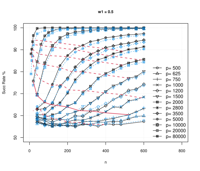
Figure 1: Balanced case $w_{1}=0.5$. We plot the success rate for various values of dimension $p$ ranging from $500$ to $80000$, as $n$ increases. Here $\gamma=0.0016$ and $1/\gamma=625$. For two lines with the same marker, the black solid line is for SDP solution $\widehat{Z}$ (and partition based on $\widehat{x}$), and the blue dashed line is for Algorithm 2. Red lines (with no markers) highlight the success rates at different levels of $np\gamma^{2}$ ranging from $0.5$ to $3.5$, from bottom to top with a step of $0.5$. The solid red line is for $np\gamma^{2}=1$. In general, $np\gamma^{2}>1$ is necessary to see a success rate larger than $60\%$, when $p\geq 625=1/{\gamma}$.

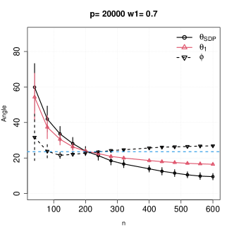
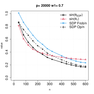
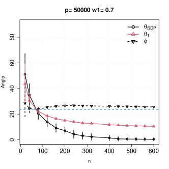
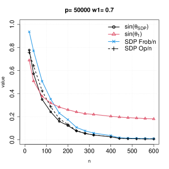
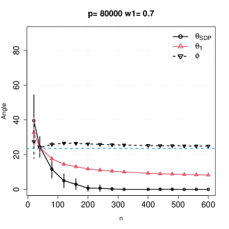
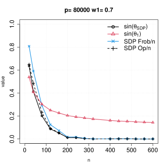
Figure 2: Imbalanced case $w_{1}=0.7$, $p\in\{20000,50000,80000\}$. Left column shows the angle $\theta_{\mathop{\text{SDP}\kern 0.54248pt}}$ (resp. $\theta_{1}$) between the leading eigenvector $\widehat{x}$ of SDP solution $\widehat{Z}$ (resp. $v_{1}$ of $YY^{T}$) and $\bar{x}$ (resp. $\bar{v}_{1}$). As $n$ increases, $\theta_{\mathop{\text{SDP}\kern 0.54248pt}}$ decreases faster than $\theta_{1}$, especially for larger values of $p$. Horizontal dashed (straight) line is the static angle $\angle(\bar{v}_{1},\bar{x})$; The dashed curve around it is for the random $\phi=\angle(\widehat{x},v_{1})$. Each vertical bar shows one standard deviation over $100$ trials. Right column plots $\sin(\theta_{\mathop{\text{SDP}\kern 0.54248pt}})$, ${\lVert Z^{*}-\widehat{Z}\rVert}_{F}/{n}$, $\lVert Z^{*}-\widehat{Z}\rVert_{2}/{n}$ for SDP, and $\sin(\theta_{1})$ for Algorithm 2.

9 Conclusion

Exploring the tradeoffs of $n$ and $p$ that are sufficient for classification, when sample size $n$ is small, is both of theoretical interests and practical value. A recent line of work establishes approximate recovery guarantees of the SDPs in the low-SNR regime for sub-gaussian mixture models; see [16, 20] among others. The present work aims to further illuminate the geometric and probabilistic features for this problem, while allowing cluster sizes and variance profiles to vary across the two populations. Although we use the population clustering problem as a motivating example, our concentration of measure analyses in Section 7, upon adaptation, will work for the general settings (6) as well. In particular, we study SDP relaxation as well as a simple spectral algorithm, which are efficiently solvable in both theoretical and practical senses, and provide a unified analysis of the two most commonly studied procedures in the literature. By doing so, we gained new insight that the leading eigenvectors not only contain sufficient information for clustering but it is also feasible to use algorithmic techniques to identify group memberships effectively once the SNR is bounded below by a constant.

Appendix A Organization

We prove Corollaries 2.6 and 2.8 in Section B. Proofs for lemmas appearing in Section 3 appear in Section C. We prove Theorem 3.5 in Section D. Proof of Theorem 4.1 appears in Section E. Proofs of Theorem 5.2 appears in Section F.1. Section G contains the concentration of measure analysis with regards to the random matrix $YY^{T}-{\mathbb{E}}(YY^{T})$, leading to Theorem 5.2. In Section H, we prove the corresponding result for Lemma 5.1. Section I contains the concentration of measure analysis for anisotropic random vectors, leading to the conclusion of Theorem 5.3. In Section I.4, we prove Theorem 7.3, the Hanson-Wright inequality for anisotropic sub-gaussian vectors, which may be of independent interests.

Appendix B Proof of Corollaries 2.6 and 2.8

Theorem B.1 is a well-known result in perturbation theory. See [9] for a proof. See also Theorem 4.5.5 [42] and Corollary 3 in [43].

Theorem B.1.

(Davis-Kahan) For $A$ and $M$ being two symmetric matrices and $E=M-A$. Let $\lambda_{1}(A)\geq\lambda_{2}(A)\geq\ldots\geq\lambda_{n}(A)$ be eigenvalues of $A$, with orthonormal eigenvectors $v_{1},v_{2},\ldots,v_{n}$ and let $\lambda_{1}(M)\geq\lambda_{2}(M)\geq\ldots\geq\lambda_{n}(M)$ be eigenvalues of $M$ and $w_{1},w_{2},\ldots,w_{n}$ be the corresponding orthonormal eigenvectors of $M$, with $\theta_{i}=\angle(v_{i},w_{i})$. Then

$$\theta_{i}\sim\sin(\theta_{i})\leq\frac{2\left\lVert E\right\rVert_{2}}{\textsf{gap}(i,A)}\;\text{ where}\;\;\textsf{gap}(i,A)=\min_{j\not=i}\left\lvert\lambda_{i}(A)-\lambda_{j}(A)\right\rvert.$$ (82)

Proof of Corollary 2.6.   See proof of Corollary 1.2 [22] for the first result, which follows from Davis-Kahan Theorem and is a direct consequence of the error bound (30), while noting that the largest eigenvalue of $\bar{x}\bar{x}^{T}$ is $n$ while all others are 0, and hence the spectral gap in the sense of Theorem B.1 equals $n$; In more details, we have by Theorem 2.5 and Corollary 3 [43],

$$\min_{\alpha=\pm 1}\left\lVert(\alpha\widehat{x}-\bar{x})/\sqrt{n}\right\rVert_{2}^{2} \leq \frac{2^{3}\left\lVert\widehat{Z}-\bar{x}\bar{x}^{T}\right\rVert_{2}^{2}}{\textsf{gap}(1,\bar{x}\bar{x}^{T})^{2}}\leq{2^{3}\left\lVert\widehat{Z}-\bar{x}\bar{x}^{T}\right\rVert_{F}^{2}}/{n^{2}}$$

$$\leq 2^{3}{4K_{G}\xi}/{w_{\min}^{2}}$$

$\;\;\scriptstyle\Box$

Proof of Corollary 2.8.   The angle between $\widehat{x}/\sqrt{n}$ and $\bar{x}/\sqrt{n}$ can be expressed as

$$\cos(\theta_{\mathop{\text{SDP}\kern 0.60275pt}})=\cos(\angle(\widehat{x},\bar{x})) = \;\langle{\,\widehat{x},\bar{x}\,}\rangle\;/n$$ (83)

The upper bound on $\sin(\theta_{\mathop{\text{SDP}\kern 0.60275pt}})$ follows from Theorems 2.7 and B.1; Moreover, by Davis-Kahan Theorem, cf. Corollary 3 [43], we have with probability at least $1-2\exp(-cn)-2/n^{2}$,

$$\min_{\alpha=\pm 1}\left\lVert(\alpha\widehat{x}-\bar{x})/\sqrt{n}\right\rVert_{2} \leq \frac{2^{3/2}\left\lVert\widehat{Z}-\bar{x}\bar{x}^{T}\right\rVert_{2}}{\textsf{gap}(1,\bar{x}\bar{x}^{T})}\leq{2^{3/2}\left\lVert\widehat{Z}-\bar{x}\bar{x}^{T}\right\rVert_{F}}/{n}$$

$$\leq 2^{3/2}(2\left\lVert\widehat{Z}-\bar{x}\bar{x}^{T}\right\rVert_{1})^{1/2}/{n}\leq 4\exp(-c_{0}s^{2}w_{\min}^{4}/2)$$

where the last inequality holds upon adjusting that constants. The corollary thus holds.  $\;\;\scriptstyle\Box$

Appendix C Proofs for results in Section 3

Combining (47), (45) and (46), we have the following Fact C.1.

Fact C.1.

(Grothendieck’s inequality, PSD) Every matrix $B\in\mathbb{R}^{n\times n}$ satisfies

$$\max_{Z\in{\mathcal{M}}_{G}^{+}}\left\lvert\;\langle{\,B,Z\,}\rangle\;\right\rvert\leq K_{G}\left\lVert B\right\rVert_{\infty\to 1}.$$

C.1 Proof of Lemma 3.3

The upper bound in (49) is trivial by definition of $Z^{*},\widehat{Z}\in{\mathcal{M}}_{\text{opt}}$ and uses the fact that $Z^{*}:=\arg\max_{Z\in{\mathcal{M}}_{\text{opt}}}\;\langle{\,R,Z\,}\rangle\;$; The lower bound depends on Fact (C.1), which implies that

$$\forall Z\in{\mathcal{M}}_{\text{opt}},\quad\left\lvert\;\langle{\,B-R,Z\,}\rangle\;\right\rvert\leq K_{G}\left\lVert B-R\right\rVert_{\infty\to 1}=:\varepsilon$$ (84)

Now to prove the lower bound in(49), we will first replace $R$ by $B$ using (84),

$$\;\langle{\,R,\widehat{Z}\,}\rangle\; \geq \;\langle{\,B,\widehat{Z}\,}\rangle\;-\varepsilon$$

$$\geq \;\langle{\,B,Z^{*}\,}\rangle\;-\varepsilon\geq\;\langle{\,R,Z^{*}\,}\rangle\;-2\varepsilon$$

where the second inequality uses the fact that $\widehat{Z}:=\arg\max_{Z\in{\mathcal{M}}_{\text{opt}}}\;\langle{\,B,Z\,}\rangle\;$, and $\widehat{Z},Z^{*}\in{\mathcal{M}}_{\text{opt}}$ by definition (48), while the last inequality holds by (84), since $Z^{*}\in{\mathcal{M}}_{\text{opt}}$ and hence

$$\left\lvert\;\langle{\,B-R,Z^{*}\,}\rangle\;\right\rvert \leq K_{G}\left\lVert B-R\right\rVert_{\infty\to 1}$$ (85)

Hence (50) holds. Finally, we prove (51); By (84), (85), and the triangle inequality, we have for all $Z\in{\mathcal{M}}_{\text{opt}}$,

$$\left\lvert\;\langle{\,B-R,Z-Z^{*}\,}\rangle\;\right\rvert \leq 2K_{G}\left\lVert B-R\right\rVert_{\infty\to 1}$$

from which (51) follows.  $\;\;\scriptstyle\Box$

C.2 Proof of Proposition 3.4

Recall

$${\mathcal{M}}_{\text{opt}} := \left\{Z:Z\succeq 0,\mathrm{diag}(Z)=I_{n}\right\}\subset{\mathcal{M}}^{+}_{G}\subset[-1,1]^{n\times n};$$

Notice that for the second term in (9), we have $\;\langle{\,(E_{n}-I_{n}),Z\,}\rangle\;=\;\langle{\,(E_{n}-I_{n}),\mathrm{offd}(Z)\,}\rangle\;$ in the objective function (11), which does not depend on $\mathrm{diag}(Z)$; Hence, to maximize

$$\;\langle{\,A,Z\,}\rangle\; = \;\langle{\,{A},\mathrm{offd}(Z)\,}\rangle\;+\;\langle{\,A,\mathrm{diag}(Z)\,}\rangle\;$$

$$= \;\langle{\,\mathrm{offd}(A),\mathrm{offd}(Z)\,}\rangle\;+\;\langle{\,\mathrm{diag}(YY^{T}),\mathrm{diag}(Z)\,}\rangle\;,$$

one must set the diagonal $Z_{jj}\in[0,1]$ to be 1, since $\mathrm{diag}(YY^{T})\geq 0$. Moreover, increasing $\mathrm{diag}(Z)$ will only make it easier to satisfy $Z\succeq 0$ and hence to maximize $\;\langle{\,\mathrm{offd}(A),\mathrm{offd}(Z)\,}\rangle\;$. Thus, the set of optimizers $\widehat{Z}$ as in (12) must satisfy $\mathrm{diag}(\widehat{Z})=I_{n}$. Thus (54) holds by definition of ${\mathcal{M}}_{\text{opt}}$ as above. Moreover, (55) holds due to the fact that $\;\langle{\,I_{n},Z\,}\rangle\;={\rm tr}(Z)=n$ for all $Z$ in the feasible set ${\mathcal{M}}_{\text{opt}}$.  $\;\;\scriptstyle\Box$

C.3 Proof of Lemma 3.6

One can check that the maximizer of $\;\langle{\,R,Z\,}\rangle\;$ on the larger set $[-1,1]^{n\times n}$, which contains the feasible set ${\mathcal{M}}_{\text{opt}}$, is $Z^{*}$. Clearly $\mathrm{diag}(Z^{*})=I_{n}$. Since $Z^{*}=\bar{x}\bar{x}^{T}\succeq 0$ belongs to the smaller set ${\mathcal{M}}_{\text{opt}}\subset M_{G}^{+}$, it must be the maximizer of $\;\langle{\,R,Z\,}\rangle\;$ on that set as well.  $\;\;\scriptstyle\Box$

C.4 Proof of Lemma 3.7

We will prove that (59) holds for all $Z\in[-1,1]^{n}\supset{\mathcal{M}}_{\text{opt}}$. Recall we have

$$R={\mathbb{E}}(Y){\mathbb{E}}(Y)^{T} =: \left\lVert\mu^{(1)}-\mu^{(2)}\right\rVert_{2}^{2}\left[\begin{array}[]{cc}w_{2}^{2}{\bf 1}_{n_{1}}\otimes{\bf 1}_{n_{1}}&-w_{1}w_{2}{\bf 1}_{n_{1}}\otimes{\bf 1}_{n_{2}}\\ -w_{1}w_{2}{\bf 1}_{n_{2}}\otimes{\bf 1}_{N_{1}}&w_{1}^{2}{\bf 1}_{n_{2}}\otimes{\bf 1}_{n_{2}}\end{array}\right]$$

$$= p\gamma\left[\begin{array}[]{cc}w_{2}^{2}E_{n_{1}}&-w_{1}w_{2}E_{n_{1}\times n_{2}}\\ -w_{1}w_{2}E_{n_{2}\times n_{1}}&w_{1}^{2}E_{n_{2}}\end{array}\right]=:p\gamma\left[\begin{array}[]{cc}\mathbb{A}&\mathbb{B}\\ \mathbb{B}^{T}&\mathbb{C}\end{array}\right]$$

Now all entries of $Z^{*},Z$ belong to $[-1,1]$. Clearly, for the upper left and lower right diagonal blocks, denoted by $\mathbb{D}=\{\mathbb{A},\mathbb{C}\}$, we have $Z^{*}-Z\geq 0$, since all entries of $Z^{*}$ on these blocks are $1$s. Similarly, for the off-diagonal blocks $\{\mathbb{B},\mathbb{B}^{T}\}$, we have $Z-Z^{*}\geq 0$ since all entries of $Z^{*}$ on these blocks are $-1$s. Thus we have

$$\frac{1}{p\gamma}\;\langle{\,R,Z^{*}-Z\,}\rangle\; = \sum_{(i,j)\in\mathbb{A}}w_{2}^{2}(Z^{*}-Z)_{ij}+\sum_{(i,j)\in\mathbb{C}}w_{1}^{2}(Z^{*}-Z)_{ij}-\sum_{(i,j)\in\mathbb{B},\mathbb{B}^{T}}w_{1}w_{2}(Z^{*}-Z)_{ij}$$

$$\geq (w_{2}^{2}\wedge w_{1}^{2}\wedge w_{1}w_{2})\big{(}\sum_{(i,j)\in\mathbb{D}}(Z^{*}-Z)+\sum_{(i,j)\in\{\mathbb{B},\mathbb{B}^{T}\}}(Z-Z^{*})_{ij}\big{)}$$

$$\geq \min_{j=1,2}w_{j}^{2}\left\lVert Z-Z^{*}\right\rVert_{1}$$

where we use the fact that

$$\sum_{(i,j)\in\mathbb{D}}(Z^{*}-Z)_{ij}+\sum_{(i,j)\in\{\mathbb{B},\mathbb{B}^{T}\}}(Z-Z^{*})_{ij} = \left\lVert Z-Z^{*}\right\rVert_{1}$$

The lemma is thus proved.  $\;\;\scriptstyle\Box$

Appendix D Proof of Theorem 3.5

We first state Lemma D.1.

Lemma D.1.

(Deterministic bounds) Let $\lambda$ and $\tau$ be as defined in (10) using matrix $Y$ as specified in Definition 2.1. By definition of $\tau$ and $\lambda$, we have

$$(n-1)\left\lvert\lambda-{\mathbb{E}}\lambda\right\rvert = \left\lvert\tau-{\mathbb{E}}\tau\right\rvert\leq\left\lVert YY^{T}-{\mathbb{E}}(YY^{T})\right\rVert_{2}$$ (87)

Proof.

Now (87) holds since $2{n\choose 2}\left\lvert\lambda-{\mathbb{E}}\lambda\right\rvert=\left\lvert n(\tau-{\mathbb{E}}\tau)\right\rvert\leq n\left\lVert YY^{T}-{\mathbb{E}}(YY^{T})\right\rVert_{2}$ where

$$\left\lvert\sum_{i=1}^{n}(\;\langle{\,Y_{i},Y_{i}\,}\rangle\;-{\mathbb{E}}\;\langle{\,Y_{i},Y_{i}\,}\rangle\;)\right\rvert=:n\left\lvert(\tau-{\mathbb{E}}\tau)\right\rvert$$

$$\leq n\max_{i}\left\lvert\;\langle{\,Y_{i},Y_{i}\,}\rangle\;-{\mathbb{E}}\;\langle{\,Y_{i},Y_{i}\,}\rangle\;\right\rvert\leq n\left\lVert YY^{T}-{\mathbb{E}}(YY^{T})\right\rVert_{2}$$

$\;\;\scriptstyle\Box$

Proof of Theorem 3.5.   We have by Theorem 5.2 (resp. Theorem 5.3), with probability at least $1-2\exp(-cn)$,

$$\left\lVert B-{\mathbb{E}}B\right\rVert_{\infty\to 1} \leq \left\lVert YY^{T}-{\mathbb{E}}(YY^{T})\right\rVert_{\infty\to 1}+\left\lvert\lambda-{\mathbb{E}}\lambda\right\rvert\left\lVert E_{n}-I_{n}\right\rVert_{\infty\to 1}$$

$$\leq \left\lVert YY^{T}-{\mathbb{E}}(YY^{T})\right\rVert_{\infty\to 1}+n\left\lVert YY^{T}-{\mathbb{E}}(YY^{T})\right\rVert_{2}\leq\frac{1}{3}\xi n^{2}p\gamma$$

where we use the fact that $\left\lVert E_{n}-I_{n}\right\rVert_{\infty\to 1}=n(n-1)$ and by Lemma D.1,

$$(n-1)\left\lvert\lambda-{\mathbb{E}}\lambda\right\rvert=\left\lvert\tau-{\mathbb{E}}\tau\right\rvert=\frac{1}{n}\left\lvert{\rm tr}(YY^{T}-{\mathbb{E}}(YY^{T}))\right\rvert\leq\left\lVert YY^{T}-{\mathbb{E}}(YY^{T})\right\rVert_{2}$$

Now $\left\lVert E_{n}-I_{n}\right\rVert_{2}\leq\left\lVert E_{n}-I_{n}\right\rVert_{\infty}=(n-1)$; and thus similarly,

$$\left\lVert B-{\mathbb{E}}B\right\rVert_{2} \leq \left\lVert YY^{T}-{\mathbb{E}}(YY^{T})\right\rVert_{2}+\left\lvert\lambda-{\mathbb{E}}\lambda\right\rvert\left\lVert E_{n}-I_{n}\right\rVert_{2}$$

$$\leq 2\left\lVert YY^{T}-{\mathbb{E}}(YY^{T})\right\rVert_{2}\leq\frac{1}{3}\xi np\gamma$$

Theorem 3.5 then holds by the triangle inequality; cf. (73) and (74), in view of Lemma 5.1. See also Lemma H.7.  $\;\;\scriptstyle\Box$

Appendix E Proof of Theorem 4.1

It is known that for any real symmetric matrix, there exist a set of $n$ orthonormal eigenvectors. First we state Fact E.1. Fact E.1 is also not surprising, since the sum of all off-diagonal entries of $A$ is 0.

Fact E.1.

Suppose that we observe one instance of the gram matrix $\widehat{S}_{n}:=XX^{T}$. Then

$$YY^{T} = (I-P_{1})XX^{T}(I-P_{1})$$ (88)

where

$$\;\langle{\,YY^{T},E_{n}\,}\rangle\;={\bf 1}^{T}_{n}YY^{T}{\bf 1}_{n}=0.$$

Moreover, by construction, we have for $A$ as defined in (9),

$$\;\langle{\,A,E_{n}\,}\rangle\; = {\bf 1}_{n}^{T}YY^{T}{\bf 1}_{n}-\lambda\;\langle{\,(E_{n}-I_{n}),E_{n}\,}\rangle\;=-\lambda n(n-1)={\rm tr}(YY^{T})$$

where

$$\lambda = \frac{1}{n(n-1)}\sum_{i\not=j}\;\langle{\,Y_{i},Y_{j}\,}\rangle\;=-\frac{1}{n(n-1)}{\rm tr}(YY^{T})=-\frac{\tau}{n-1}$$

In other words, we have $\;\langle{\,A,P_{1}\,}\rangle\;=\;\langle{\,A,{\bf 1}_{n}{\bf 1}_{n}^{T}/n\,}\rangle\;={\rm tr}(YY^{T})/n=:\tau$

Recall that $R$ is rank one with $\lambda_{\max}(R)={\rm tr}(R)=w_{1}w_{2}np\gamma$ while $\bar{x}R\bar{x}/n=(4w_{1}w_{2})w_{1}w_{2}np\gamma\leq\frac{1}{4}np\gamma$. Hence $\bar{x}/\sqrt{n}$ coincides with $\bar{v}_{1}$ when $w_{1}=w_{2}=1/2$. Hence for $\textsf{gap}(1,R)$, as defined in Theorem B.1,

$$\textsf{gap}(1,R)=\lambda_{\max}(R)=w_{1}w_{2}np\gamma.$$

We check the claim that the leading eigenvector of $B$ coincides with that of $YY^{T}$ in Fact E.2. Clearly,

$$\cos(\theta_{1})=\cos(\angle({v}_{1},\bar{v}_{1})) = \;\langle{\,v_{1},\bar{v}_{1}\,}\rangle\;$$ (89)

and hence

$$\theta_{1}=\arccos(\;\langle{\,v_{1},\bar{v}_{1}\,}\rangle\;).$$

Hence we can use the first eigenvector of $YY^{T}$ to partition the two groups of points in $\mathbb{R}^{p}$. To obtain an upper bound on $\sin(\theta_{1})$, we apply the Davis-Kahan perturbation bound as follows. Since $v_{1},\bar{v}_{1}$ are the leading eigenvectors of $B$ and $R$ respectively, (69) holds by Theorems 3.5 and B.1:

$$\sin(\theta_{1}) := \sin(\angle({v}_{1},\bar{v}_{1}))\leq\frac{2\left\lVert B-R\right\rVert_{2}}{\lambda_{\max}(R)}=\frac{2\left\lVert B-R\right\rVert_{2}}{w_{1}w_{2}np\gamma}\leq\frac{2\xi}{w_{1}w_{2}}.$$

Moreover, we have (70) holds by Corollary 3 [43]: since

$$\min_{\alpha=\pm 1}\left\lVert\alpha v_{1}-\bar{v}_{1}\right\rVert_{2}^{2} \leq \left(\frac{2^{3/2}\left\lVert B-R\right\rVert_{2}}{w_{1}w_{2}np\gamma}\right)^{2}$$

$$\leq \frac{2^{3}\xi^{2}}{(w_{1}w_{2})^{2}}=:\delta^{\prime},\text{ where}\;\;\delta^{\prime}={8\xi^{2}}/{(w_{1}^{2}w_{2}^{2})}\leq c_{2}\xi^{2}/w_{\min}^{2};$$

The theorem thus holds.  $\;\;\scriptstyle\Box$

It remains to state Fact E.2.

Fact E.2.

Let $YY^{T}=\sum_{j=1}^{n-1}\lambda_{j}v_{j}v_{j}^{T}$. Denote by $\widetilde{A}=YY^{T}-\lambda E_{n}$, then

$$\widetilde{A} := YY^{T}-\lambda E_{n}=\sum_{j=1}^{n-1}\lambda_{j}v_{j}v_{j}^{T}+\frac{n\tau}{n-1}{\bf 1}{\bf 1}^{T}/n\succeq 0;$$ (90)

The leading eigenvector of $\widetilde{A}$ (resp. $A$ and $B$) will coincide with that of $YY^{T}$ with

$$\lambda_{\max}(\widetilde{A}) = \lambda_{\max}(YY^{T})\geq n\tau/(n-1)$$ (91)

where strict inequality holds if and only if not all eigenvalues of $YY^{T}$ are identical. Thus the symmetric matrices $A=\widetilde{A}+\lambda I_{n}$ and $B=A+{\mathbb{E}}\tau I_{n}$ also share the same leading eigenvector $v_{1}$ with $YY^{T}$, so long as not all eigenvalues of $YY^{T}$ are identical, with $\lambda_{\max}(A)\geq\tau$.

Proof.

Clearly, the additional terms involving $E_{n}$ and $I_{n}$ are either orthogonal to eigenvectors $v_{1},\ldots,v_{n-1}$ of $YY^{T}$, or act as an identity map on the subspace spanned by $\{v_{1},\ldots,v_{n-1}\}$. Now (90) holds since $\;\langle{\,v_{j},{\bf 1}_{n}\,}\rangle\;=0$ for all $j$ and hence $\{v_{1},\ldots,v_{n-1},{\bf 1}_{n}/\sqrt{n}\}$ forms the set of orthonormal eigenvectors for $\widetilde{A}$ (resp. $A$ and $B$); and moreover, in view of Fact E.1,

$$-\lambda E_{n} = \frac{n\tau}{n-1}P_{1}=\frac{n\tau}{n-1}{\bf 1}_{n}{\bf 1}_{n}^{T}/n,\;\;\text{ where }\;\;\lambda=-\frac{\tau}{n-1},$$

Since we have at most $n-1$ non-zero eigenvalues and they sum up to be ${\rm tr}(YY^{T})$, we have

$$\lambda_{\max}(YY^{T}) \geq {\rm tr}(YY^{T})/(n-1)=n\tau/(n-1)$$

where strict inequality holds when these eigenvalues are not all identical.

Finally, (91) holds since $\lambda_{1}(\widetilde{A}):=\lambda_{\max}(YY^{T})$ in view of the eigen-decomposition (90) and the displayed equation immediately above. Now for $A=YY^{T}-\lambda(E_{n}-I_{n})$, we have ${\rm tr}(A)={\rm tr}(YY^{T})$, and hence $\lambda_{\max}(A)\geq\tau$. Moreover, the extra terms $\propto I_{n}$ in $A$ (resp. $B$) will not change the order of the sequence of eigenvalues for $B$ (resp. $A$) with respect to that established for $\widetilde{A}$; Hence all symmetric matrices $B$, $\widetilde{A}$, and $A$ share the same leading eigenvector $v_{1}$ with $YY^{T}$.  $\;\;\scriptstyle\Box$

Appendix F Proofs for results in Section 5

Proposition F.1 holds regardless of the weights or the number of mixture components.

Proposition F.1.

(Covariance projection: general mixture models) Let $Y=X-P_{1}X$ be as defined in Definition 2.1. Let ${\mathbb{Z}}=X-{\mathbb{E}}X$. We first rewrite $\widehat{\Sigma}_{Y}=(Y-{\mathbb{E}}(Y))(Y-{\mathbb{E}}(Y))^{T}$ as follows:

$$\widehat{\Sigma}_{Y} := (I-P_{1}){\mathbb{Z}}{\mathbb{Z}}^{T}(I-P_{1})=M_{1}-(M_{2}-M_{3}),$$ (92)

$$\;\;\text{ where }\;M_{1} := \widehat{\Sigma}_{X}=(X-{\mathbb{E}}(X))(X-{\mathbb{E}}(X))^{T}={\mathbb{Z}}{\mathbb{Z}}^{T},\;\;\text{ and}\;\;P_{1}=\frac{1}{n}{\bf 1}_{n}{\bf 1}_{n}^{T}$$ (93)

$$M_{2} = {\mathbb{Z}}{\mathbb{Z}}^{T}P_{1}+P_{1}{\mathbb{Z}}{\mathbb{Z}}^{T},\;\text{and}\;M_{3}=P_{1}{\mathbb{Z}}{\mathbb{Z}}^{T}P_{1},$$ (94)

$$\text{ and}\;\;\Sigma_{Y} := {\mathbb{E}}\widehat{\Sigma}_{Y}:=(I-P_{1}){\mathbb{E}}({\mathbb{Z}}{\mathbb{Z}}^{T})(I-P_{1})$$ (95)

Then we have (75), since

$$YY^{T}-{\mathbb{E}}(Y){\mathbb{E}}(Y)^{T} = \widehat{\Sigma}_{Y}+{\mathbb{E}}(Y)(Y-{\mathbb{E}}(Y))^{T}+(Y-{\mathbb{E}}(Y))({\mathbb{E}}(Y))^{T}.$$

Proof.

Recall ${\bf 1}(X)=\frac{1}{n}{\bf 1}_{n}{\bf 1}_{n}^{T}X=:P_{1}X$; Then

$$\widehat{\Sigma}_{Y}:=(Y-{\mathbb{E}}Y)(Y-{\mathbb{E}}Y)^{T} = (X-{\mathbb{E}}(X)-({\bf 1}{(X)}-{\mathbb{E}}{\bf 1}{(X)}))(X-{\mathbb{E}}(X)-({\bf 1}{(X)}-{\mathbb{E}}{\bf 1}{(X)}))^{T}$$

$$= (X-P_{1}X-({\mathbb{E}}(X)-P_{1}{\mathbb{E}}X))(X-P_{1}X-({\mathbb{E}}(X)-P_{1}{\mathbb{E}}X))^{T}$$

$$= \big{(}(I-P_{1})(X-{\mathbb{E}}(X)\big{)}\big{(}(I-P_{1})(X-{\mathbb{E}}(X))\big{)}^{T}$$

$$= (I-P_{1})(X-{\mathbb{E}}(X))(X-{\mathbb{E}}(X))^{T}(I-P_{1})$$

$$= (I-P_{1}){\mathbb{Z}}{\mathbb{Z}}^{T}(I-P_{1})$$

The rest are obvious.  $\;\;\scriptstyle\Box$

F.1 Proof of Theorem 5.2

We use a shorthand notation for $M_{Y}:={\mathbb{E}}(Y)(Y-{\mathbb{E}}(Y))^{T}+(Y-{\mathbb{E}}(Y))({\mathbb{E}}(Y))^{T}$. Thus we have by the triangle inequality,  (75), (75) (Proposition F.1), Lemma 6.1, and Theorem 6.3, with probability at least $1-2\exp(-c_{6}n)-2\exp(-cn)$,

$$\left\lVert YY^{T}-{\mathbb{E}}(YY^{T})\right\rVert_{2} \leq \left\lVert\widehat{\Sigma}_{Y}-\Sigma_{Y}\right\rVert_{2}+\left\lVert M_{Y}\right\rVert_{2}\leq\left\lVert{\mathbb{Z}}{\mathbb{Z}}^{T}-{\mathbb{E}}({\mathbb{Z}}{\mathbb{Z}}^{T})\right\rVert_{2}+\left\lVert M_{Y}\right\rVert_{2}$$

$$\leq C_{2}C_{0}^{2}(\sqrt{pn}\vee n)+2C_{3}C_{0}n\sqrt{p\gamma}\leq\frac{1}{6}\xi np\gamma$$

$$\left\lVert YY^{T}-{\mathbb{E}}(YY^{T})\right\rVert_{\infty\to 1} \leq n\left\lVert YY^{T}-{\mathbb{E}}(YY^{T})\right\rVert_{2}\leq\frac{1}{6}\xi n^{2}p\gamma$$

where the last inequality holds by (29), while adjusting the constants.  $\;\;\scriptstyle\Box$

F.2 Proof of Lemma 5.4

First, we verify (22):

$$\forall i\in{\mathcal{C}}_{1}\;\;{\mathbb{E}}Y_{i} = {\mathbb{E}}X_{i}-(w_{1}\mu^{(1)}+w_{2}\mu^{(2)})=\mu^{(1)}(1-w_{1})-w_{2}\mu^{(2)}$$ (97)

$$= w_{2}(\mu^{(1)}-\mu^{(2)})$$

$$\forall i\in{\mathcal{C}}_{2}\;\;{\mathbb{E}}Y_{i} = {\mathbb{E}}X_{i}-(w_{1}\mu^{(1)}+w_{2}\mu^{(2)})=\mu^{(2)}(1-w_{2})-w_{1}\mu^{(1)}$$ (98)

$$= w_{1}(\mu^{(2)}-\mu^{(1)})$$

Lemma F.2.

Suppose all conditions in Lemma 5.4 hold. Then

$$\sup_{q\in\mathbb{S}^{n-1}}\sum_{i=1}^{n}q_{i}\;\langle{\,Y_{i}-{\mathbb{E}}(Y_{i}),\mu^{(1)}-\mu^{(2)}\,}\rangle\; \leq 2\sup_{q\in\mathbb{S}^{n-1}}\sum_{i=1}^{n}q_{i}\;\langle{\,{\mathbb{Z}}_{i},\mu^{(1)}-\mu^{(2)}\,}\rangle\;.$$ (99)

Proof.

$$\sum_{i=1}^{n}q_{i}\;\langle{\,Y_{i}-{\mathbb{E}}(Y_{i}),\mu^{(1)}-\mu^{(2)}\,}\rangle\;=\frac{1}{n}\sum_{i=1}^{n}q_{i}\;\langle{\,\sum_{j\not=i}({\mathbb{Z}}_{i}-{\mathbb{Z}}_{j}),\mu^{(1)}-\mu^{(2)}\,}\rangle\;$$

$$= \frac{n-1}{n}\left(\sum_{i=1}^{n}q_{i}\;\langle{\,{\mathbb{Z}}_{i},\mu^{(1)}-\mu^{(2)}\,}\rangle\;\right)+\frac{1}{n}\sum_{i=1}^{n}q_{i}\;\langle{\,{\mathbb{Z}}_{i}-\sum_{j=1}^{n}{\mathbb{Z}}_{j},\mu^{(1)}-\mu^{(2)}\,}\rangle\;$$

$$= \sum_{i=1}^{n}q_{i}\;\langle{\,{\mathbb{Z}}_{i},\mu^{(1)}-\mu^{(2)}\,}\rangle\;-\frac{1}{n}\sum_{i=1}^{n}q_{i}\sum_{j=1}^{n}\;\langle{\,{\mathbb{Z}}_{j},\mu^{(1)}-\mu^{(2)}\,}\rangle\;$$

where

$$\left\lvert\frac{1}{n}\sum_{i=1}^{n}q_{i}\sum_{j=1}^{n}\;\langle{\,{\mathbb{Z}}_{j},\mu^{(1)}-\mu^{(2)}\,}\rangle\;\right\rvert\leq\sup_{q\in\mathbb{S}^{n-1}}\frac{1}{n}\left\lVert q\right\rVert_{1}\left\lvert\sum_{j=1}^{n}\;\langle{\,{\mathbb{Z}}_{j},\mu^{(1)}-\mu^{(2)}\,}\rangle\;\right\rvert$$

$$\leq \left\lvert\sum_{j=1}^{n}\frac{1}{\sqrt{n}}\;\langle{\,{\mathbb{Z}}_{j},\mu^{(1)}-\mu^{(2)}\,}\rangle\;\right\rvert\leq\sup_{q\in\mathbb{S}^{n-1}}\sum_{i=1}^{n}q_{i}\;\langle{\,{\mathbb{Z}}_{i},\mu^{(1)}-\mu^{(2)}\,}\rangle\;$$

Thus (99) holds and the lemma is proved.  $\;\;\scriptstyle\Box$

Proof of Lemma 5.4 .   Due to the symmetry, we need to compute only

$$\left\lVert(Y-{\mathbb{E}}(Y)){\mathbb{E}}(Y)^{T}\right\rVert = \left\lVert({\mathbb{Z}}-({\bf 1}{(X)}-{\mathbb{E}}{\bf 1}{(X)}))({\mathbb{E}}(X)-{\mathbb{E}}{\bf 1}{(X)})^{T}\right\rVert$$

First, we show that (76) holds. Now

$$Y_{i}-{\mathbb{E}}Y_{i} = (X_{i}-{\mathbb{E}}X_{i})-((\widehat{\mu}_{n}-{\mathbb{E}}\widehat{\mu}_{n})={\mathbb{Z}}_{i}-\left(\frac{1}{n}\sum_{i=1}^{n}(X_{i}-{\mathbb{E}}X_{i})\right)$$

$$= \frac{n-1}{n}{\mathbb{Z}}_{i}-\frac{1}{n}\sum_{j\not=i}^{n}{\mathbb{Z}}_{j}=\frac{1}{n}\sum_{j\not=i}^{n}({\mathbb{Z}}_{i}-{\mathbb{Z}}_{j})$$

and for $x_{i}\in\{-1,1\}$,

$$\sum_{i=1}^{n}x_{i}\;\langle{\,Y_{i}-{\mathbb{E}}Y_{i},\mu^{(1)}-\mu^{(2)}\,}\rangle\;=\frac{1}{n}\sum_{i=1}^{n}x_{i}\sum_{j\not=i}^{n}\;\langle{\,({\mathbb{Z}}_{i}-{\mathbb{Z}}_{j}),\mu^{(1)}-\mu^{(2)}\,}\rangle\;$$

$$\leq \frac{1}{n}\sum_{i=1}^{n}\sum_{j\not=i}^{n}\left\lvert\;\langle{\,({\mathbb{Z}}_{i}-{\mathbb{Z}}_{j}),\mu^{(1)}-\mu^{(2)}\,}\rangle\;\right\rvert\leq\frac{2(n-1)}{n}\sum_{i=1}^{n}\left\lvert\;\langle{\,{\mathbb{Z}}_{i},\mu^{(1)}-\mu^{(2)}\,}\rangle\;\right\rvert$$

Then we have by definition of the cut norm, (97), (98), and (76),

$$\left\lVert(Y-{\mathbb{E}}(Y)){\mathbb{E}}(Y)^{T}\right\rVert_{\infty\to 1}=\sup_{x,y\in\{-1,1\}^{n}}\sum_{i=1}^{n}x_{i}\cdot$$

$$\left(\sum_{j\in{\mathcal{C}}_{1}}y_{j}\;\langle{\,Y_{i}-{\mathbb{E}}(Y_{i}),w_{2}(\mu^{(1)}-\mu^{(2)})\,}\rangle\;+\sum_{j\in{\mathcal{C}}_{2}}y_{j}\;\langle{\,Y_{i}-{\mathbb{E}}(Y_{i}),w_{1}(\mu^{(2)}-\mu^{(1)})\,}\rangle\;\right)$$

$$\leq \sup_{x,y\in\{-1,1\}^{n}}\sum_{i=1}^{n}x_{i}\left(\;\langle{\,Y_{i}-{\mathbb{E}}(Y_{i}),\mu^{(1)}-\mu^{(2)}\,}\rangle\;(\sum_{j\in{\mathcal{C}}_{1}}w_{2}y_{j}-\sum_{j\in{\mathcal{C}}_{2}}w_{1}y_{j})\right)$$

$$\leq (w_{2}\left\lvert{\mathcal{C}}_{1}\right\rvert+w_{1}\left\lvert{\mathcal{C}}_{2}\right\rvert)\sum_{i=1}^{n}\left\lvert\;\langle{\,Y_{i}-{\mathbb{E}}(Y_{i}),\mu^{(1)}-\mu^{(2)}\,}\rangle\;\right\rvert$$

$$= 2w_{2}w_{1}n\max_{x\in\{-1,1\}^{n}}\sum_{i=1}^{n}x_{i}\;\langle{\,Y_{i}-{\mathbb{E}}(Y_{i}),\mu^{(1)}-\mu^{(2)}\,}\rangle\;$$

$$\leq 4w_{1}w_{2}(n-1)\sum_{i=1}^{n}\left\lvert\;\langle{\,{\mathbb{Z}}_{i},\mu^{(1)}-\mu^{(2)}\,}\rangle\;\right\rvert$$

Similarly, we have by (97) and (98),

$$\left\lVert(Y-{\mathbb{E}}(Y)){\mathbb{E}}(Y)^{T}\right\rVert_{2}=\sup_{q,h\in\mathbb{S}^{n-1}}\sum_{i=1}^{n}q_{i}\cdot$$ (100)

$$\left(\sum_{j\in{\mathcal{C}}_{1}}h_{j}\;\langle{\,Y_{i}-{\mathbb{E}}(Y_{i}),w_{2}(\mu^{(1)}-\mu^{(2)})\,}\rangle\;+\sum_{j\in{\mathcal{C}}_{2}}h_{j}\;\langle{\,Y_{i}-{\mathbb{E}}(Y_{i}),w_{1}(\mu^{(2)}-\mu^{(1)})\,}\rangle\;\right)$$

$$\leq \sup_{q,h\in\mathbb{S}^{n-1}}\left(\sum_{i=1}^{n}q_{i}\;\langle{\,Y_{i}-{\mathbb{E}}(Y_{i}),\mu^{(1)}-\mu^{(2)}\,}\rangle\;(\sum_{j\in{\mathcal{C}}_{1}}w_{2}h_{j}-\sum_{j\in{\mathcal{C}}_{2}}w_{1}h_{j})\right)=:Q$$

where by (100) and (99), and $w_{1}w_{2}\leq 1/4$,

$$Q \leq \sup_{q\in\mathbb{S}^{n-1}}\left\lvert\sum_{i=1}^{n}q_{i}\;\langle{\,Y_{i}-{\mathbb{E}}(Y_{i}),\mu^{(1)}-\mu^{(2)}\,}\rangle\;\right\rvert\cdot\sup_{h\in\mathbb{S}^{n-1}}\left\lvert\sum_{j\in{\mathcal{C}}_{1}}w_{2}h_{j}-\sum_{j\in{\mathcal{C}}_{2}}w_{1}h_{j}\right\rvert$$

$$\leq 2\sup_{q\in\mathbb{S}^{n-1}}\left\lvert\sum_{i=1}^{n}q_{i}\;\langle{\,{\mathbb{Z}}_{i},\mu^{(1)}-\mu^{(2)}\,}\rangle\;\right\rvert\cdot\sqrt{nw_{1}w_{2}}\leq\sqrt{n}\sup_{q\in\mathbb{S}^{n-1}}\left\lvert\;\langle{\,\sum_{i}q_{i}{\mathbb{Z}}_{i},\mu^{(1)}-\mu^{(2)}\,}\rangle\;\right\rvert$$

where for $\left\lVert h_{{\mathcal{C}}_{i}}\right\rVert_{2}=\sqrt{\sum_{j\in{\mathcal{C}}_{i}}h^{2}_{j}},i=1,2$ and $h\in\mathbb{S}^{n-1}$,

$$\left\lvert\sum_{j\in{\mathcal{C}}_{1}}w_{2}h_{j}-\sum_{j\in{\mathcal{C}}_{2}}w_{1}h_{j}\right\rvert \leq w_{2}\sum_{j\in{\mathcal{C}}_{1}}\left\lvert h_{j}\right\rvert+w_{1}\sum_{j\in{\mathcal{C}}_{2}}\left\lvert h_{j}\right\rvert=:w_{2}\left\lVert h_{{\mathcal{C}}_{1}}\right\rVert_{1}+w_{1}\left\lVert h_{{\mathcal{C}}_{2}}\right\rVert_{1}$$

$$\leq w_{2}\sqrt{\left\lvert{\mathcal{C}}_{1}\right\rvert}\left\lVert h_{{\mathcal{C}}_{1}}\right\rVert_{2}+w_{1}\sqrt{\left\lvert{\mathcal{C}}_{2}\right\rvert}\left\lVert h_{{\mathcal{C}}_{2}}\right\rVert_{2}$$

$$\leq \sqrt{w_{1}w_{2}n}\left(\sqrt{w_{2}}\left\lVert h_{{\mathcal{C}}_{1}}\right\rVert_{2}+\sqrt{w_{1}}\left\lVert h_{{\mathcal{C}}_{2}}\right\rVert_{2}\right)\leq\sqrt{w_{1}w_{2}n}$$

where $1=w_{1}+w_{2}\geq 2\sqrt{w_{1}w_{2}}$ and by Cauchy-Schwarz, we have for $\bar{w_{0}}=(\sqrt{w_{2}},\sqrt{w_{1}})$ such that $\left\lVert\bar{w_{0}}\right\rVert_{2}=\sqrt{w_{1}+w_{2}}=1$ and $z=(\left\lVert h_{{\mathcal{C}}_{1}}\right\rVert_{2},\left\lVert h_{{\mathcal{C}}_{2}}\right\rVert_{2})$ such that $\left\lVert z\right\rVert_{2}=1$,

$$\;\langle{\,\bar{w_{0}},z\,}\rangle\;=\left(\sqrt{w_{2}}\left\lVert h_{{\mathcal{C}}_{1}}\right\rVert_{2}+\sqrt{w_{1}}\left\lVert h_{{\mathcal{C}}_{2}}\right\rVert_{2}\right)\leq\left\lVert w_{0}\right\rVert_{2}\left\lVert z\right\rVert_{2}=1.$$

$\;\;\scriptstyle\Box$

F.3 Proof of Lemma 5.5

Reduction in the operator norm holds since by Proposition F.1,

$$\widehat{\Sigma}_{Y}-\Sigma_{Y} := (Y-{\mathbb{E}}Y)(Y-{\mathbb{E}}Y)^{T}-{\mathbb{E}}((Y-{\mathbb{E}}Y)(Y-{\mathbb{E}}Y)^{T})$$

$$= (I-P_{1})({\mathbb{Z}}{\mathbb{Z}}^{T}-{\mathbb{E}}({\mathbb{Z}}{\mathbb{Z}}^{T}))(I-P_{1})$$

and clearly,

$$\left\lVert\widehat{\Sigma}_{Y}-\Sigma_{Y}\right\rVert_{2} \leq \left\lVert I-P_{1}\right\rVert_{2}\left\lVert{\mathbb{Z}}{\mathbb{Z}}^{T}-{\mathbb{E}}({\mathbb{Z}}{\mathbb{Z}}^{T})\right\rVert_{2}\left\lVert I-P_{1}\right\rVert_{2}$$

$$\leq \left\lVert{\mathbb{Z}}{\mathbb{Z}}^{T}-{\mathbb{E}}({\mathbb{Z}}{\mathbb{Z}}^{T})\right\rVert_{2}.$$

$\;\;\scriptstyle\Box$

Appendix G Proofs for Section 6 on isotropic design

Under (A2), the row vectors ${\mathbb{Z}}_{1},{\mathbb{Z}}_{2},\ldots,{\mathbb{Z}}_{n}\in\mathbb{R}^{p}$ of matrix ${\mathbb{Z}}=X-{\mathbb{E}}X$, are independent, sub-gaussian vectors with sub-gaussian norm, cf. Lemma 3.4.2 [42]. To bridge the deterministic bounds in Lemma 5.4 and the probabilistic statements in Lemma 6.1, we use the tail bounds in Lemma 6.2. Combining Lemmas 5.4 and 6.2 proves Lemma 6.1.

G.1 Proof of Lemma 6.1

Let $\varepsilon=1/3$. Let $\Pi_{n}$ be an $\varepsilon$-net of $\mathbb{S}^{n-1}$ such that $\left|\Pi_{n}\right|\leq(1+2/\varepsilon)^{n}$; We have by (79) and the union bound,

$$\mathbb{P}\left({\mathbb{E}}_{3}\right) := \mathbb{P}\left(\left\lvert\sup_{q\in\Pi_{n}}\sum_{i=1}^{n}q_{i}\;\langle{\,{\mathbb{Z}}_{i},\mu\,}\rangle\;\right\rvert\geq\frac{1}{2}C_{3}C_{0}\sqrt{n}\right)$$

$$\leq 9^{n}\cdot 2\exp\left(-c_{6}{C_{3}^{2}n}/{4}\right)\leq 2\exp(-c_{1}n)$$

for some absolute constants $C_{3},c_{1}$ and $\mu$ as in (77). Thus we have on event ${\mathbb{E}}_{3}^{c}$, by a standard approximation argument,

$$\sup_{q\in\mathbb{S}^{n-1}}\sum_{i=1}^{n}q_{i}\;\langle{\,{\mathbb{Z}}_{i},\mu\,}\rangle\; \leq \frac{1}{1-\varepsilon}\sup_{q\in\Pi_{n}}\sum_{i=1}^{n}q_{i}\;\langle{\,{\mathbb{Z}}_{i},\mu\,}\rangle\;\leq C_{3}C_{0}\sqrt{n}$$

Similarly, we have by the union bound and (78),

$$\mathbb{P}\left({\mathbb{E}}_{4}\right) := \mathbb{P}\left(\max_{u\in\{-1,1\}^{n}}\left\lvert\sum_{i=1}^{n}u_{i}\;\langle{\,{\mathbb{Z}}_{i},\mu\,}\rangle\;\right\rvert\geq\frac{1}{2}C_{4}C_{0}n\right)$$

$$\leq 2^{n}\exp\left(-c_{5}\frac{(C_{4}C_{0})^{2}n^{2}}{4C_{0}^{2}n}\right)\leq 2\exp(-c^{\prime}n);$$

Hence on ${\mathbb{E}}_{4}^{c}$, the second inequality follows from (76).

$$\sup_{u\in\{-1,1\}^{n}}\sum_{i=1}^{n}u_{i}\;\langle{\,Y_{i}-{\mathbb{E}}Y_{i},\mu\,}\rangle\; \leq \frac{2(n-1)}{n}\sup_{u\in\{-1,1\}^{n}}\sum_{i=1}^{n}u_{i}\;\langle{\,{\mathbb{Z}}_{i},\mu\,}\rangle\;\leq C_{4}C_{0}(n-1)$$

We have by Lemma 5.4, on event ${\mathbb{E}}_{3}^{c}\cap{\mathbb{E}}_{4}^{c}$,

$$\left\lVert M_{Y}\right\rVert_{2} \leq 4\sqrt{n}\sqrt{w_{1}w_{2}}\sup_{q\in S^{n-1}}\left\lvert\sum_{i}q_{i}\;\langle{\,{\mathbb{Z}}_{i},\mu^{(1)}-\mu^{(2)}\,}\rangle\;\right\rvert\leq 2C_{3}C_{0}n\sqrt{p\gamma}$$

and

$$\left\lVert M_{Y}\right\rVert_{\infty\to 1} \leq 8w_{1}w_{2}(n-1)\sup_{u\in\{-1,1\}^{n}}\sum_{i=1}^{n}u_{i}\;\langle{\,{\mathbb{Z}}_{i},\mu^{(1)}-\mu^{(2)}\,}\rangle\;\leq C_{4}C_{0}n(n-1)\sqrt{p\gamma}$$

Thus the lemma holds upon adjusting the constants.  $\;\;\scriptstyle\Box$

G.2 Proof of Lemma 6.2

Let $\mu$ be as in (77) and recall

$$\max_{i}\left\lVert{\mathbb{Z}}_{i}\right\rVert_{\psi_{2}}\leq CC_{0}$$

Moreover, by independence of ${\mathbb{Z}}_{1},\ldots,{\mathbb{Z}}_{n}$, we have for $u=(u_{1},\ldots,u_{n})\in\{-1,1\}^{n}$,

$$\left\lVert\sum_{i=1}^{n}u_{i}\;\langle{\,{\mathbb{Z}}_{i},\mu\,}\rangle\;\right\rVert^{2}_{\psi_{2}} \leq C\sum_{i=1}^{n}\left\lVert\;\langle{\,{\mathbb{Z}}_{i},\mu\,}\rangle\;\right\rVert^{2}_{\psi_{2}}\leq C\sum_{i=1}^{n}\left\lVert{\mathbb{Z}}_{i}\right\rVert^{2}_{\psi_{2}}$$

where $\left\lVert\;\langle{\,{\mathbb{Z}}_{j},\mu\,}\rangle\;\right\rVert_{\psi_{2}}\leq\left\lVert{\mathbb{Z}}_{j}\right\rVert_{\psi_{2}}$ by definition of (13), and for any $q\in\mathbb{S}^{n-1}$ and $t>0$, we have

$$\left\lVert\sum_{i=1}^{n}q_{i}\;\langle{\,{\mathbb{Z}}_{i},\mu\,}\rangle\;\right\rVert^{2}_{\psi_{2}}\leq C\sum_{i=1}^{n}q_{i}^{2}\left\lVert\;\langle{\,{\mathbb{Z}}_{i},\mu\,}\rangle\;\right\rVert^{2}_{\psi_{2}}\leq C\max_{i}\left\lVert{\mathbb{Z}}_{i}\right\rVert^{2}_{\psi_{2}}\leq C^{\prime}C_{0}^{2}$$

Thus we have the following sub-gaussian tail bounds, for any $u=(u_{1},\ldots,u_{n})\in\{-1,1\}^{n}$ and $t>0$,

$$\mathbb{P}\left(\sum_{i=1}^{n}u_{i}\;\langle{\,{\mathbb{Z}}_{i},\mu\,}\rangle\;\geq t\right) \leq 2\exp\left(-\frac{ct^{2}}{\sum_{i=1}^{n}\left\lVert{\mathbb{Z}}_{i}\right\rVert^{2}_{\psi_{2}}}\right)\leq 2\exp\left(-\frac{ct^{2}}{C_{0}^{2}n}\right)$$

and for any $q\in\mathbb{S}^{n-1}$ and $t>0$,

$$\mathbb{P}\left(\sum_{i=1}^{n}q_{i}\;\langle{\,{\mathbb{Z}}_{i},\mu\,}\rangle\;\geq t\right) \leq 2\exp\left(-\frac{ct^{2}}{\max_{i=1}^{n}\left\lVert{\mathbb{Z}}_{i}\right\rVert^{2}_{\psi_{2}}}\right)\leq 2\exp\left(-\frac{c^{\prime}t^{2}}{C_{0}^{2}}\right)$$

See Proposition 2.5.2 (i) [42]. Thus the lemma holds.  $\;\;\scriptstyle\Box$

G.3 Proof sketch of Theorem 6.3

First, notice that $M_{1}={\mathbb{Z}}{\mathbb{Z}}^{T}=:\widehat{\Sigma}_{X}$ is the empirical covariance matrix based on the original data $X$. In order to prove the concentration of measure bounds for Theorem 6.3, we will first state the operator norm bound on $M_{1}-{\mathbb{E}}M_{1}$ in Lemma G.1.

Let $C_{\mathrm{diag}},C_{\mathrm{offd}},C_{1},C_{2},c,c^{\prime},\ldots$ be some absolute constants, which may change line by line. Denote by ${\mathbb{E}}_{0}$ the following event:

$${\mathbb{E}}_{0}: \exists j\in[n]\quad\left\lvert\left\lVert{\mathbb{Z}}_{j}\right\rVert_{2}^{2}-{\mathbb{E}}\left\lVert{\mathbb{Z}}_{j}\right\rVert_{2}^{2}\right\rvert>C_{\mathrm{diag}}C_{0}^{2}(\sqrt{np}\vee n)$$ (104)

Lemma G.1.

(M1 term: operator norm) Choose $\varepsilon=1/4$ and construct an $\varepsilon$-net ${\mathcal{N}}$ whose size is upper bounded by $\left\lvert{\mathcal{N}}\right\rvert\leq(\frac{2}{\varepsilon}+1)^{n}\leq 9^{n}$. Recall that ${\mathbb{Z}}=X-{\mathbb{E}}X$. Fix $\varepsilon=1/4$. Under the conditions in Theorem 6.3, denote by ${\mathbb{E}}_{8}$ the following event:

$$\text{ event }{\mathbb{E}}_{8}:\quad\left\{\max_{q,h\in{\mathcal{N}}}\sum_{i=1}^{n}\sum_{j\not=i}^{n}\;\langle{\,{\mathbb{Z}}_{i},{\mathbb{Z}}_{j}\,}\rangle\;q_{i}h_{j}>C_{1}C_{0}^{2}(\sqrt{np}\vee n)\right\}$$

As a consequence, on event ${\mathbb{E}}_{0}^{c}\cap{\mathbb{E}}_{8}^{c}$, we have

$$\left\lVert{\mathbb{Z}}{\mathbb{Z}}^{T}-{\mathbb{E}}{\mathbb{Z}}{\mathbb{Z}}^{T}\right\rVert_{2} \leq C_{2}C_{0}^{2}(\sqrt{np}\vee n)$$

where $\mathbb{P}\left({\mathbb{E}}_{0}^{c}\cap{\mathbb{E}}_{8}^{c}\right)\geq 1-2\exp(-c_{4}n)$, upon adjusting the constants.

When we take ${\mathbb{Z}}$ as a sub-gaussian ensemble with independent entries, our bounds on $\left\lVert M_{1}-{\mathbb{E}}M_{1}\right\rVert$ (cut norm and operator norm) depend on the Bernstein’s type of inequalities and higher dimensional Hanson-Wright inequalities. We will state Lemma G.4 in Section G.4, where we bound the probability of event ${\mathbb{E}}_{0}$. We prove Lemma G.1 in Section G.5 using the standard net argument. Neither weights, nor the number of mixture components, will affect such bounds.

G.4 Bounds on independent sub-exponential random variables

We now derive the corresponding bounds using properties of sub-exponential random variables. The sub-exponential (or $\psi_{1}$) norm of random variable $S$, denoted by $\left\lVert S\right\rVert_{\psi_{1}}$, is defined as

$$\left\lVert S\right\rVert_{\psi_{1}}=\inf\{t>0\;:\;{\mathbb{E}}\exp(\left\lvert S\right\rvert/t)\leq 2\}.$$ (105)

A random variable $Z$ is sub-gaussian if and only if $S:=Z^{2}$ is sub-exponential with $\left\lVert S\right\rVert_{\psi_{1}}=\left\lVert Z\right\rVert^{2}_{\psi_{2}}$.

The proof does not depend on the specific sizes $\left\lvert{\mathcal{C}}_{j}\right\rvert\forall j$ of clusters. Lemma G.2 concerns the sum of independent sub-exponential random variables. We also state the Hanson-Wright inequality [40].

Lemma G.2.

(Bernstein’s inequality, cf. Theorem 2.8.1 [42]) Let $X_{1},\ldots,X_{n}$ be independent, mean-zero, sub-exponential random variables. Then for every $t>0$,

$$\mathbb{P}\left(\left\lvert\sum_{j=1}^{n}X_{j}\right\rvert\geq t\right) \leq 2n\exp\left(-c\min\left(\frac{t^{2}}{\sum_{j=1}^{n}\left\lVert X_{j}\right\rVert^{2}_{\psi_{1}}},\frac{t}{\max_{j}\left\lVert X_{j}\right\rVert_{\psi_{1}}}\right)\right)$$

Theorem G.3.

[40] Let $X=(X_{1},\ldots,X_{m})\in\mathbb{R}^{m}$ be a random vector with independent components $X_{i}$ which satisfy ${\mathbb{E}}X_{i}=0$ and $\left\lVert X_{i}\right\rVert_{\psi_{2}}\leq C_{0}$. Let $A$ be an $m\times m$ matrix. Then, for every $t>0$,

$$\mathbb{P}\left(\left\lvert X^{T}AX-{\mathbb{E}}(X^{T}AX)\right\rvert>t\right)\leq 2\exp\left(-c\min\left(\frac{t^{2}}{C_{0}^{4}\left\lVert A\right\rVert_{F}^{2}},\frac{t}{C_{0}^{2}\left\lVert A\right\rVert_{2}}\right)\right).$$

Lemma G.4.

Let ${\mathbb{Z}}=(z_{jk})\in\mathbb{R}^{n\times p}$ be a random matrix whose entries are independent, mean-zero, sub-gaussian random variables with $\max_{j,k}\left\lVert z_{jk}\right\rVert_{\psi_{2}}\leq C_{0}$. Then we have for $t_{\mathrm{diag}}=C_{\mathrm{diag}}C_{0}^{2}(\sqrt{np}\vee n)$,

$$\mathbb{P}\left({\mathbb{E}}_{0}\right) := \mathbb{P}\left(\exists j\in[n],\quad\left\lvert\left\lVert{\mathbb{Z}}_{j}\right\rVert_{2}^{2}-{\mathbb{E}}\left\lVert{\mathbb{Z}}_{j}\right\rVert_{2}^{2}\right\rvert>t_{\mathrm{diag}}\right)\leq 2\exp(-c_{0}n)$$

where $\{{\mathbb{Z}}_{j},j\in[n]\}$ are row vectors of matrix ${\mathbb{Z}}$, and $C_{\mathrm{diag}}$ and $c_{0}$ are absolute constants.

Proof.

Denote by

$$S_{jk}=z_{jk}^{2}-{\mathbb{E}}z_{jk}^{2},\quad\text{where}\;z_{jk}=X_{jk}-{\mathbb{E}}X_{jk},\forall i\in[n],k\in[p]$$ (106)

It follows from (105) that $S_{jk}$ is a mean-zero, sub-exponential random variable since

$$\max_{j,k}\left\lVert S_{jk}\right\rVert_{\psi_{1}} \leq CC_{0}^{2}\;\;\;\text{ since}\;\;\forall j,k,\;\left\lVert z^{2}_{jk}\right\rVert_{\psi_{1}}=\left\lVert z_{jk}\right\rVert^{2}_{\psi_{2}}\leq C_{0}^{2},$$

$$\text{ and }\;\left\lVert S_{jk}\right\rVert_{\psi_{1}} = \left\lVert z^{2}_{jk}-{\mathbb{E}}z^{2}_{jk}\right\rVert_{\psi_{1}}\leq C\left\lVert z_{jk}^{2}\right\rVert_{\psi_{1}}=C\left\lVert z_{jk}\right\rVert^{2}_{\psi_{2}}\leq CC_{0}^{2}$$

See Exercise 2.7.10 [42]. Set $t_{3}=C_{\mathrm{diag}}C_{0}^{2}\sqrt{np}\vee n$. We have by Bernstein’s inequality Lemma G.2 and the union bound, the following large deviation bound:

$$\mathbb{P}\left(\exists j\in[n],\quad\left\lvert\left\lVert{\mathbb{Z}}_{j}\right\rVert_{2}^{2}-{\mathbb{E}}\left\lVert{\mathbb{Z}}_{j}\right\rVert_{2}^{2}\right\rvert\geq t_{3}\right)\leq\sum_{j=1}^{n}\mathbb{P}\left(\left\lvert\sum_{k=1}^{p}S_{jk}\right\rvert\geq t_{3}\right)\leq$$ (107)

$$2n\exp\left(-c\min\left(\frac{(C_{\mathrm{diag}}C_{0}^{2}\sqrt{np}\vee n)^{2}}{\max_{j\in[n]}\sum_{k=1}^{p}\left\lVert S_{jk}\right\rVert^{2}_{\psi_{1}}},\frac{C_{\mathrm{diag}}C_{0}^{2}\sqrt{np}\vee n}{\max_{j,k}\left\lVert S_{jk}\right\rVert_{\psi_{1}}}\right)\right)$$

$$\leq 2n\exp\left(-c\min\left(\frac{C^{2}_{\mathrm{diag}}np}{p},C_{\mathrm{diag}}n\right)\right)\leq 2\exp(-c_{0}n)$$

where for all ${j\in[n]}$, $\sum_{k=1}^{p}\left\lVert S_{jk}\right\rVert^{2}_{\psi_{1}}\leq pC^{2}C_{0}^{4}$. The lemma thus holds.  $\;\;\scriptstyle\Box$

G.5 Proof of Lemma G.1

We use Theorem G.3 to bound the off-diagonal part. Recall $\max_{j,k}\left\lVert z_{jk}\right\rVert_{\psi_{2}}\leq C_{0}$. Let $\rm{vec}\left\{\,{\mathbb{Z}}\,\right\}=\rm{vec}\left\{\,X-{\mathbb{E}}X\,\right\}$ be formed by concatenating columns of matrix ${\mathbb{Z}}$ into a long vector of size $np$. For a particular realization of $q,h\in\mathbb{S}^{n-1}$, we construct a block-diagonal matrix $\widetilde{A}(q,h)$, where $\mathrm{diag}(\widetilde{A})=0$, with $p$ identical block-diagonal coefficient matrices $A_{qh}^{(k)}=\mathrm{offd}(q\otimes h),\forall k$ of size $n\times n$ along the diagonal. Then

$$\left\lvert\sum_{i=1}^{n}q_{i}\sum_{j\not=i}^{n}h_{j}\;\langle{\,{\mathbb{Z}}_{i},{\mathbb{Z}}_{j}\,}\rangle\;\right\rvert := \left\lvert\rm{vec}\left\{\,{\mathbb{Z}}\,\right\}^{T}\widetilde{A}_{q,h}\rm{vec}\left\{\,{\mathbb{Z}}\,\right\}\right\rvert$$

and

$$\forall q,h\in\mathbb{S}^{n-1},\quad\left\lVert\widetilde{A}(q,h)\right\rVert_{F}^{2} = \sum_{k=1}^{p}\left\lVert A_{qh}^{(k)}\right\rVert_{F}^{2}=p\left\lVert\mathrm{offd}(q\otimes h)\right\rVert_{F}^{2}\leq p,$$

$$\left\lVert\widetilde{A}(q,h)\right\rVert_{2} = \left\lVert\mathrm{offd}(q\otimes h)\right\rVert_{2}\leq 1,$$

$$\text{ since }\;\;\left\lVert\mathrm{offd}(q\otimes h)\right\rVert_{2} \leq \left\lVert\mathrm{offd}(q\otimes h)\right\rVert_{F}\leq\left\lVert q\otimes h\right\rVert_{F}^{2}={\rm tr}(qh^{T}hq^{T})=1.$$

Taking a union bound over all $\left\lvert{\mathcal{N}}\right\rvert^{2}$ pairs $q,h\in{\mathcal{N}}$, the $\varepsilon$-net of $\mathbb{S}^{n-1}$, we have by Theorem G.3, for some sufficiently large constants $C_{1}$ and $c>4\ln 9$,

$$\mathbb{P}\left({\mathbb{E}}_{8}\right):=\mathbb{P}\left(\max_{q,h\in{\mathcal{N}}}\left\lvert\sum_{i=1}^{n}\sum_{j\not=i}^{n}q_{i}h_{j}\;\langle{\,{\mathbb{Z}}_{i},{\mathbb{Z}}_{j}\,}\rangle\;\right\rvert>C_{1}C_{0}^{2}(\sqrt{pn}\vee n)\right)$$

$$\leq \left\lvert{\mathcal{N}}\right\rvert^{2}\mathbb{P}\left(\left\lvert\rm{vec}\left\{\,{\mathbb{Z}}\,\right\}^{T}\widetilde{A}(q,h)\rm{vec}\left\{\,{\mathbb{Z}}\,\right\}\right\rvert>C_{1}C_{0}^{2}(\sqrt{pn}\vee n)\right)$$

$$\leq 2\times 9^{2n}\exp\left(-c\min\left({C_{1}^{2}pn}/{p},{C_{1}n}\right)\right)$$

$$\leq 2\exp\left(-cn+2n\ln 9\right)=2\exp\left(-c_{3}n\right)$$

A standard approximation argument shows that under ${\mathbb{E}}_{8}^{c}$, we have

$$\left\lVert\mathrm{offd}({\mathbb{Z}}{\mathbb{Z}}^{T})\right\rVert_{2} = \sup_{q\in\mathbb{S}^{n-1}}\sum_{i=1}^{n}\sum_{j\not=i}^{n}q_{i}q_{j}\;\langle{\,{\mathbb{Z}}_{i},{\mathbb{Z}}_{j}\,}\rangle\;$$

$$\leq \frac{1}{(1-2\varepsilon)}\sup_{q,h\in{\mathcal{N}}}\sum_{i=1}^{n}\sum_{j\not=i}^{n}q_{i}h_{j}\;\langle{\,{\mathbb{Z}}_{i},{\mathbb{Z}}_{j}\,}\rangle\;\leq 2C_{1}C_{0}^{2}(\sqrt{np}\vee n)$$

See for example Exercise 4.4.3 [42].

The large deviation bound on the operator norm follows from the triangle inequality: on event ${\mathbb{E}}_{8}^{c}\cap{\mathbb{E}}_{0}^{c}$,

$$\left\lVert{\mathbb{Z}}{\mathbb{Z}}^{T}-{\mathbb{E}}({\mathbb{Z}}{\mathbb{Z}}^{T})\right\rVert_{2} \leq \left\lVert\mathrm{diag}({\mathbb{Z}}{\mathbb{Z}}^{T}-{\mathbb{E}}({\mathbb{Z}}{\mathbb{Z}}^{T}))\right\rVert_{2}+\left\lVert\mathrm{offd}({\mathbb{Z}}{\mathbb{Z}}^{T})\right\rVert_{2}\leq C_{2}C_{0}^{2}(\sqrt{np}\vee n)$$

for some absolute constant $C_{2}$.  $\;\;\scriptstyle\Box$

Appendix H Bias terms

This section proves results needed for Theorem 3.5. We prove Lemmas 5.1 in Section H.2, where we also state Lemma H.7. Combining (139), (140), and Proposition H.4, we obtain an expression on ${\mathbb{E}}B-R$. Recall $R={\mathbb{E}}(Y){\mathbb{E}}(Y)^{T}$ is as defined in (25). We have the following facts about $R$.

Fact H.1.

When we sum over all entries in $R$, clearly, we have for $R$ as defined in (25), ${\bf 1}^{T}_{n}R{\bf 1}_{n}=0$,

$${\bf 1}^{T}_{n}\mathrm{offd}(R){\bf 1}_{n} = {\bf 1}^{T}_{n}R{\bf 1}_{n}-{\rm tr}(R)=-{\rm tr}(R)=-np\gamma w_{2}w_{1},\;\text{ where}$$ (108)

$$\frac{1}{p\gamma}{\rm tr}(R) = nw_{2}^{2}w_{1}+nw_{1}^{2}w_{2}=w_{1}w_{2}n\quad\text{ and hence }\quad\left\lVert R\right\rVert_{2}={\rm tr}(R)=w_{1}w_{2}np\gamma$$

Lemma H.2.

We have by Fact H.1, ${{\rm tr}(R)}/{n}=p\gamma w_{1}w_{2}$ and hence for $n\geq 4$,

$$\left\lVert\frac{{\rm tr}(R)}{n-1}\left(I_{n}-{E_{n}}/{n}\right)\right\rVert_{2} \leq \frac{n}{n-1}o\gamma w_{1}w_{2}\leq p\gamma/3$$ (109)

$$\text{ and hence }\quad\left\lVert\frac{{\rm tr}(R)}{n-1}\left(I_{n}-{E_{n}}/{n}\right)\right\rVert_{\infty\to 1} \leq \frac{n}{n-1}np\gamma w_{1}w_{2}\leq np\gamma/3$$ (110)

where $\left\lVert I_{n}-{E_{n}}/{n}\right\rVert_{\infty\to 1}\leq n\left\lVert I_{n}-{E_{n}}/{n}\right\rVert_{2}=1$ since $I_{n}-{E_{n}}/{n}$ is a projection matrix.

H.1 Some useful propositions

Next, we compute the mean values in Proposition H.3, and we obtain an expression on ${\mathbb{E}}B-R$ in Proposition H.4. Proposition H.3 is proved in Section H.3.

Proposition H.3.

(Covariance projection: two groups) Let $N_{j}=w_{j}n$ for $j\in\{1,2\}$. W.l.o.g., suppose that the first $N_{1}$ rows in $X$ are in ${\mathcal{C}}_{1}$ and the following $N_{2}$ rows are in ${\mathcal{C}}_{2}$. Let $M_{1},M_{2},M_{3}$ be defined as in Proposition F.1. Let $V_{1}$ and $V_{2}$ be the same as in (28):

$$V_{1}:={\mathbb{E}}\;\langle{\,{\mathbb{Z}}_{j},{\mathbb{Z}}_{j}\,}\rangle\;\;\;\forall j\in{\mathcal{C}}_{1}\;\;\text{ and }\;\;V_{2}:={\mathbb{E}}\;\langle{\,{\mathbb{Z}}_{j},{\mathbb{Z}}_{j}\,}\rangle\;\;\;\forall j\in{\mathcal{C}}_{2}$$ (111)

Let $V_{m}:=w_{1}V_{1}+w_{2}V_{2}=W_{n}/n$. Let $\widehat{\Sigma}_{Y}$ be as in (92). Let $W_{n}$ be defined as in (112):

$$W_{n} := {\mathbb{E}}\sum_{i=1}^{n}\;\langle{\,{\mathbb{Z}}_{i},{\mathbb{Z}}_{i}\,}\rangle\;=\sum_{i=1}^{n}\sum_{k=1}^{p}{\mathbb{E}}z_{ik}^{2}.$$ (112)

Then

$${\mathbb{E}}M_{1} = \left[\begin{array}[]{cc}V_{1}I_{N_{1}}&0\\ 0&V_{2}I_{N_{2}}\end{array}\right]=:(w_{1}V_{1}+w_{2}V_{2})I_{n}+W_{0},$$ (115)

$${\mathbb{E}}M_{2} = \frac{V_{1}+V_{2}}{n}E_{n}+W_{2},$$ (116)

$${\mathbb{E}}M_{3} := {\mathbb{E}}\;\langle{\,\widehat{\mu}_{n}-{\mathbb{E}}\widehat{\mu}_{n},\widehat{\mu}_{n}-{\mathbb{E}}\widehat{\mu}_{n}\,}\rangle\;{\bf 1}_{n}\otimes{\bf 1}_{n}=\frac{W_{n}}{n^{2}}E_{n},$$ (117)

$$\text{ and }\;\;W_{n}/n^{2} := (\left\lvert{\mathcal{C}}_{1}\right\rvert V_{1}+\left\lvert{\mathcal{C}}_{2}\right\rvert V_{2})/n^{2}=(w_{1}V_{1}+w_{2}V_{2})/n=:\frac{V_{w}}{n},$$ (118)

where ${\rm tr}({\mathbb{E}}M_{1})/n=V_{m}$ and

$$W_{0} = (V_{1}-V_{2})\left[\begin{array}[]{cc}w_{2}I_{N_{1}}&0\\ 0&-w_{1}I_{N_{2}}\end{array}\right]\;\;\text{and}\;\;W_{2}:=\frac{V_{1}-V_{2}}{n}\left[\begin{array}[]{cc}E_{N_{1}}&0\\ 0&-E_{N_{2}}\end{array}\right].$$ (123)

Now putting things together, we obtain the expression for covariance of $Y$:

$$\Sigma_{Y}:={\mathbb{E}}(YY^{T})-{\mathbb{E}}(Y){\mathbb{E}}(Y)^{T}={\mathbb{E}}M_{1}+{\mathbb{E}}M_{3}-{\mathbb{E}}M_{2}$$

$$= \left[\begin{array}[]{cc}V_{1}I_{N_{1}}&0\\ 0&V_{2}I_{N_{2}}\end{array}\right]-\frac{w_{2}V_{1}+w_{1}V_{2}}{n}E_{n}-W_{2}\;$$

which simplifies to

$$\Sigma_{Y}=V(I_{n}-E_{n}/n)\;\text{ in case }\;\;V_{1}=V_{2}=V$$

We prove Proposition H.4 in Section H.4. Intuitively, $W_{2}$ and $\mathbb{W}$ arise due to the imbalance in variance profiles.

Proposition H.4.

(Bias decomposition) Let $M_{1},M_{2},M_{3}$, $W_{0}$, $W_{2}$, $V_{1},V_{2}...$ be the same as in Propositions F.1 and H.3. Then

$${\mathbb{E}}B-R = W_{0}-\mathbb{W}-\frac{{\rm tr}(R)}{(n-1)}(I_{n}-\frac{E_{n}}{n})\;\text{ where}\;\;$$ (125)

$$\mathbb{W} := W_{2}+\frac{(V_{1}-V_{2})(w_{2}-w_{1})}{n}E_{n}$$ (126)

where for $W_{2}$ defined in (123). Moreover, when $V_{1}=V_{2}$, $W_{0}=\mathbb{W}=0$.

Next, we state the following fact about $W_{2}$.

Fact H.5.

Denote by

$$\mathbb{W}:=W_{2}-\frac{1}{n}{\rm tr}(W_{2})I_{n}-\frac{{\bf 1}_{n}^{T}\mathrm{offd}(W_{2}){\bf 1}_{n}}{n(n-1)}(E_{n}-I_{n})$$

Then $\mathbb{W}$ coincides with (126). Moreover, we have

$$\mathbb{W} = W_{2}-\frac{(V_{2}-V_{1})(w_{2}-w_{1})}{n}E_{n}$$

$$:= \frac{V_{1}-V_{2}}{n}\left[\begin{array}[]{cc}2w_{2}E_{N_{1}}&(w_{2}-w_{1})E_{N_{1}\times N_{2}}\\ (w_{2}-w_{1})E_{N_{1}\times N_{2}}&-2w_{1}E_{N_{2}}\end{array}\right]$$

Moreover, we have

$$\left\lVert\mathbb{W}\right\rVert_{2} \leq \left\lvert V_{1}-V_{2}\right\rvert(w_{1}\vee w_{2})\;\text{ and }\;\;\left\lVert\mathbb{W}\right\rVert_{\infty\to 1}\leq n\left\lvert V_{1}-V_{2}\right\rvert(w_{1}\vee w_{2})$$ (128)

Proof.

By definition of $W_{2}$ as in (123), we have

$${\rm tr}(W_{2}) = \frac{V_{2}-V_{1}}{n}(w_{2}n-w_{1}n)=(V_{2}-V_{1})(w_{2}-w_{1})\;\text{ and }$$

$${\bf 1}_{n}^{T}W_{2}{\bf 1}_{n} = \frac{V_{2}-V_{1}}{n}(w^{2}_{2}n^{2}-w_{1}^{2}n^{2})=n(V_{2}-V_{1})(w^{2}_{2}-w^{2}_{1})$$

$$= n(V_{2}-V_{1})(w_{2}-w_{1})$$

Thus

$$\frac{{\bf 1}_{n}^{T}\mathrm{offd}(W_{2}){\bf 1}_{n}}{n(n-1)} = \frac{{\bf 1}_{n}^{T}W_{2}{\bf 1}_{n}-{\rm tr}(W_{2})}{n(n-1)}=\frac{(V_{2}-V_{1})(w_{2}-w_{1})}{n};$$

Then

$$\mathbb{W} = W_{2}-\frac{1}{n}{\rm tr}(W_{2})I_{n}-\frac{{\bf 1}_{n}^{T}\mathrm{offd}(W_{2}){\bf 1}_{n}}{n(n-1)}(E_{n}-I_{n})$$

$$= W_{2}-\frac{(V_{2}-V_{1})(w_{2}-w_{1})}{n}E_{n}.$$

Hence (126) holds. Moreover, by symmetry, $\left\lVert\mathbb{W}\right\rVert_{2}\leq\left\lVert\mathbb{W}\right\rVert_{\infty}\leq\left\lvert V_{1}-V_{2}\right\rvert(w_{1}\vee w_{2}).$  $\;\;\scriptstyle\Box$

H.2 Proof of Lemma 5.1

We have by Proposition H.4,

$$\left\lVert{\mathbb{E}}B-R\right\rVert = \left\lVert W_{0}-\mathbb{W}-\frac{{\rm tr}(R)}{(n-1)}(I_{n}-\frac{E_{n}}{n})\right\rVert$$ (129)

$$\leq \left\lVert W_{0}\right\rVert+\left\lVert\mathbb{W}\right\rVert+\left\lVert\frac{{\rm tr}(R)}{(n-1)}(I_{n}-\frac{E_{n}}{n})\right\rVert$$

where the $\left\lVert\cdot\right\rVert$ is understood to be either the operator or the cut norm. Recall that

$$W_{0} := {\mathbb{E}}M_{1}-V_{w}I_{n}=(V_{1}-V_{2})\left[\begin{array}[]{cc}w_{2}I_{w_{1}n}&0\\ 0&-w_{1}I_{w_{2}n}\end{array}\right]$$

$$\text{ and hence}\;\;{\bf 1}^{T}_{n}W_{0}{\bf 1}_{n} = {\rm tr}(W_{0})=0\;\;\text{and}\;\;V_{m}:={\rm tr}({\mathbb{E}}M_{1})/n=w_{1}V_{1}+w_{2}V_{2}$$

and hence $W_{0}$ disappears if the two clusters have identical sum of variances: $V_{1}=V_{2}$. Clearly,

$$\left\lVert W_{0}\right\rVert_{2} \leq \left\lvert V_{1}-V_{2}\right\rvert(w_{2}\vee w_{1})$$ (131)

Combining (129), (131), (128), and (110), we have for $w_{\min}:=w_{1}\wedge w_{2}$ and $n\xi\geq\frac{1}{2w_{\min}}$

$$\left\lVert{\mathbb{E}}B-R\right\rVert_{2} \leq \left\lVert W_{0}\right\rVert_{2}+\left\lVert\mathbb{W}\right\rVert_{2}+\left\lVert\frac{{\rm tr}(R)}{(n-1)}(I_{n}-\frac{E_{n}}{n})\right\rVert_{2}$$

$$\leq 2\left\lvert V_{1}-V_{2}\right\rvert(w_{1}\vee w_{2})+p\gamma/3$$

$$= \frac{2}{3}\xi np\gamma(1-w_{\min})+p\gamma/3\leq\frac{2}{3}\xi np\gamma$$

where we use the fact that

$$\frac{2}{3}\xi p\gamma nw_{\min}\geq p\gamma/3\;\;\text{ since }\;\;2\xi nw_{\min}\geq 1$$

Now the bound on the cut norm follows since

$$\left\lVert{\mathbb{E}}B-R\right\rVert_{\infty\to 1} \leq n\left\lVert{\mathbb{E}}B-R\right\rVert_{2}\leq\frac{2}{3}\xi n^{2}p\gamma$$

The lemma thus holds for the general setting; when $V_{1}=V_{2}$, we show the improved bounds in Lemma H.7.  $\;\;\scriptstyle\Box$

Corollary H.6 follows from the proof of Lemma 5.1, which we state to prove a bound for the balanced cases. The proof is given in Section H.5.

Corollary H.6.

For general cases, we have by definition,

$$W_{2} := \frac{V_{1}-V_{2}}{n}\left[\begin{array}[]{cc}E_{N_{1}}&0E_{N_{1}\times N_{2}}\\ 0E_{N_{1}\times N_{2}}&-E_{N_{2}}\end{array}\right]$$

Moreover we have the following term which depends on the weights,

$$\left\lVert\frac{(V_{2}-V_{1})(w_{2}-w_{1})}{n}E_{n}\right\rVert_{\infty\to 1} \leq n\left\lvert(V_{2}-V_{1})(w_{2}-w_{1})\right\rvert\leq\xi n^{2}p\gamma\left\lvert w_{2}-w_{1}\right\rvert$$

$$\left\lVert W_{2}\right\rVert_{\infty\to 1} := n\left\lvert V_{1}-V_{2}\right\rvert(w_{1}^{2}+w_{2}^{2})$$

$$\text{ and hence }\;\;\left\lVert W_{0}-W_{2}\right\rVert_{\infty\to 1} \leq n\left\lVert W_{0}-W_{2}\right\rVert_{2}<n\left\lvert V_{1}-V_{2}\right\rvert\leq\xi pn^{2}\gamma$$

Lemma H.7.

(Reductions) Let $W_{0},W_{2},V_{1},V_{2}$ be the same as in Proposition H.3. Recall that $R={\mathbb{E}}(Y){\mathbb{E}}(Y)^{T}$. When $V_{1}=V_{2}$, we have

$${\mathbb{E}}B-R=-\frac{{\rm tr}(R)}{(n-1)}(I_{n}-\frac{E_{n}}{n})=-p\gamma w_{2}w_{1}\frac{n}{n-1}(I_{n}-\frac{E_{n}}{n})$$

and hence for $n\geq 4$,

$$\left\lVert{\mathbb{E}}B-R\right\rVert_{\infty\to 1}=\left\lVert p\gamma w_{2}w_{1}\frac{n}{n-1}(I_{n}-\frac{E_{n}}{n})\right\rVert_{\infty\to 1}\leq np\gamma/3$$

For balanced clusters, that is, when $w_{1}=w_{2}$, we have

$${\mathbb{E}}B-R = W_{0}-W_{2}-\frac{{\rm tr}(R)}{(n-1)}(I_{n}-\frac{E_{n}}{n})$$

and hence for $n\geq 4$,

$$\left\lVert{\mathbb{E}}B-R\right\rVert_{2} \leq \frac{p\gamma}{3}+\left\lvert V_{1}-V_{2}\right\rvert\leq\frac{1}{3}(1+o(1))\xi pn\gamma$$

$$\left\lVert{\mathbb{E}}B-R\right\rVert_{\infty\to 1} \leq \frac{np\gamma}{3}+\left\lvert V_{1}-V_{2}\right\rvert n\leq\frac{1}{3}(1+o(1))\xi pn^{2}\gamma.$$

Proof.

Recall

$$W_{0}-W_{2} = (V_{1}-V_{2})\left[\begin{array}[]{cc}w_{2}I_{N_{1}}-E_{N_{1}}/n&0\\ 0&-(w_{1}I_{N_{2}}-E_{N_{2}}/n)\end{array}\right]$$

The case where $V_{1}=V_{2}$ follows from Lemma H.2 and (125). We now show the balanced case where $w_{1}=w_{2}$. Under the conditions of Lemma 5.1, we have for $\xi=\Omega(1/n)$, by (109) and (125),

$$\left\lVert{\mathbb{E}}B-R\right\rVert_{2} \leq \left\lVert W_{0}-W_{2}\right\rVert_{2}+\left\lVert\frac{(V_{1}-V_{2})(w_{1}-w_{2})}{n}E_{n}\right\rVert_{2}+\left\lVert\frac{{\rm tr}(R)}{n-1}\left(I_{n}-{E_{n}}/{n}\right)\right\rVert_{2}$$

$$\leq \left\lvert V_{1}-V_{2}\right\rvert+p\gamma/3\leq\frac{1}{3}\xi np\gamma+p\gamma/3$$

Similarly, we obtain

$$\left\lVert{\mathbb{E}}B-R\right\rVert_{\infty\to 1} \leq \left\lvert V_{1}-V_{2}\right\rvert n+np\gamma/3\leq\frac{1}{3}\xi n^{2}p\gamma+np\gamma/3$$

The proof follows from Corollary H.6 immediately.  $\;\;\scriptstyle\Box$

H.3 Proof of Proposition H.3

Denote by ${\rm tr}({\mathbb{E}}M_{1})/n=(w_{1}V_{1}+w_{2}V_{2})=V_{m}$.

$${\mathbb{E}}M_{1} = {\mathbb{E}}\left((X-{\mathbb{E}}(X))(X-{\mathbb{E}}(X))^{T}\right)={\mathbb{E}}{\mathbb{Z}}{\mathbb{Z}}^{T}$$

$$= \left[\begin{array}[]{cc}V_{1}I_{w_{1}n}&0\\ 0&V_{2}I_{w_{2}n}\end{array}\right]$$

Moreover, upon subtracting the component of $V_{w}I_{n}=\frac{1}{n}{\rm tr}({\mathbb{E}}M_{1})I_{n}$ from ${\mathbb{E}}M_{1}$, we have $W_{0}$:

$${\mathbb{E}}M_{1}-V_{w}I_{n} := {\mathbb{E}}M_{1}-\frac{1}{n}{\rm tr}({\mathbb{E}}M_{1})I_{n}=(V_{1}-V_{2})\left[\begin{array}[]{cc}w_{2}I_{w_{1}n}&0\\ 0&-w_{1}I_{w_{2}n}\end{array}\right]=:W_{0};$$

Next we evaluate ${\mathbb{E}}M_{2}$: for ${\mathbb{Z}}=X-{\mathbb{E}}X$

$${\mathbb{E}}M_{2} = {\mathbb{E}}\left(\left({\mathbb{Z}}({\bf 1}{(X)}-{\mathbb{E}}{\bf 1}{(X)})^{T}+({\bf 1}{(X)}-{\mathbb{E}}{\bf 1}{(X)}){\mathbb{Z}}^{T}\right)\right)$$

$$= \frac{1}{n}\left[\begin{array}[]{cc}2V_{1}E_{N_{1}}&(V_{1}+V_{2})E_{N_{1}\times N_{2}}\\ (V_{1}+V_{2})E_{N_{1}\times N_{2}}&2V_{2}E_{N_{2}}\end{array}\right]$$

$$\text{and hence}\quad{\mathbb{E}}M_{2}-\frac{(V_{1}+V_{2})}{n}E_{n} = \frac{V_{1}-V_{2}}{n}\left[\begin{array}[]{cc}E_{N_{1}}&0E_{N_{1}\times N_{2}}\\ 0E_{N_{1}\times N_{2}}&-E_{N_{2}}\end{array}\right]=:W_{2}$$

For $W_{n}$ as defined in (112), we have

$${\mathbb{E}}\;\langle{\,\widehat{\mu}_{n}-{\mathbb{E}}\widehat{\mu}_{n},\widehat{\mu}_{n}-{\mathbb{E}}\widehat{\mu}_{n}\,}\rangle\; := \frac{1}{n^{2}}\sum_{i=1}^{n}\sum_{k}{\mathbb{E}}z_{ik}^{2}=\frac{w_{1}V_{1}+w_{2}V_{2}}{n}=\frac{V_{m}}{n}$$

$${\mathbb{E}}M_{3} := {\mathbb{E}}\;\langle{\,\widehat{\mu}_{n}-{\mathbb{E}}\widehat{\mu}_{n},\widehat{\mu}_{n}-{\mathbb{E}}\widehat{\mu}_{n}\,}\rangle\;E_{n}=\frac{\left\lvert{\mathcal{C}}_{1}\right\rvert V_{1}+\left\lvert{\mathcal{C}}_{2}\right\rvert V_{2}}{n^{2}}E_{n}=\frac{W_{n}}{n^{2}}E_{n}$$

Now putting things together,

$${\mathbb{E}}(YY^{T})-{\mathbb{E}}(Y){\mathbb{E}}(Y)^{T}={\mathbb{E}}M_{1}+{\mathbb{E}}M_{3}-{\mathbb{E}}M_{2}$$

$$= \left[\begin{array}[]{cc}V_{1}I_{N_{1}}&0\\ 0&V_{2}I_{N_{2}}\end{array}\right]+\frac{V_{m}}{n}E_{n}-\frac{(V_{1}+V_{2})}{n}E_{n}-W_{2}\;\;\;\text{ where}$$

$$\frac{V_{m}}{n}-\frac{(V_{1}+V_{2})}{n} = -\frac{V_{1}(1-w_{1})+V_{2}(1-w_{2})}{n}=-\frac{V_{1}w_{2}+V_{2}w_{1}}{n}$$

The proposition thus holds.  $\;\;\scriptstyle\Box$

H.4 Proof of Proposition H.4

First, we have by Proposition F.1, and $R={\mathbb{E}}(Y){\mathbb{E}}(Y)^{T}$,

$${\mathbb{E}}(YY^{T})=\Sigma_{Y}+R={\mathbb{E}}M_{1}-{\mathbb{E}}M_{2}+{\mathbb{E}}M_{3}+R$$ (138)

We have by Fact H.1 and (138),

$${\mathbb{E}}\tau = \frac{1}{n}\sum_{i=1}^{n}{\mathbb{E}}\;\langle{\,Y_{i},Y_{i}\,}\rangle\;={\mathbb{E}}{\rm tr}(YY^{T})/n={\rm tr}({\Sigma}_{Y})/n+{\rm tr}(R)/n$$ (139)

$$= \frac{1}{n}\left({\rm tr}({\mathbb{E}}M_{1}+{\mathbb{E}}M_{3})-{\rm tr}({\mathbb{E}}M_{2})\right)+{\rm tr}(R)/n$$

$${\mathbb{E}}\lambda = \frac{1}{n(n-1)}\sum_{i\not=j}^{n}{\mathbb{E}}\;\langle{\,Y_{i},Y_{j}\,}\rangle\;=\frac{1}{n(n-1)}{\bf 1}_{n}^{T}{\mathbb{E}}(\mathrm{offd}(YY^{T})){\bf 1}_{n}$$ (140)

$$= \frac{1}{n(n-1)}{\bf 1}_{n}^{T}\mathrm{offd}({\mathbb{E}}M_{3}-{\mathbb{E}}M_{2}){\bf 1}_{n}-\frac{{\rm tr}(R)}{n(n-1)}$$

where in (140) we use the fact that $\mathrm{offd}({\mathbb{E}}M_{1})=0$ by (116) and (108). Hence by definition of $B$ and $R$, we have

$${\mathbb{E}}B-R = {\mathbb{E}}M_{1}-{\mathbb{E}}M_{2}+{\mathbb{E}}M_{3}-{\mathbb{E}}\tau I_{n}-{\mathbb{E}}\lambda(E_{n}-I_{n})$$ (141)

$$= {\mathbb{E}}M_{1}-{\mathbb{E}}M_{2}+{\mathbb{E}}M_{3}-\left(\frac{1}{n}{\rm tr}({\mathbb{E}}M_{1}+{\mathbb{E}}M_{3})-\frac{1}{n}{\rm tr}({\mathbb{E}}M_{2})+\frac{{\rm tr}(R)}{n}\right)I_{n}$$

$$-\left(\frac{1}{n(n-1)}{\bf 1}_{n}^{T}\mathrm{offd}({\mathbb{E}}M_{1}+{\mathbb{E}}M_{3}-{\mathbb{E}}M_{2}){\bf 1}_{n}-\frac{{\rm tr}(R)}{n(n-1)}\right)(E_{n}-I_{n})$$

• Notice that ${\mathbb{E}}M_{3}=\frac{V_{w}}{n}E_{n}$ and hence its contribution to ${\mathbb{E}}\tau$ and ${\mathbb{E}}\lambda$ is the same; Thus we have

  $${\rm tr}({\mathbb{E}}M_{3}) = \frac{1}{(n-1)}{\bf 1}_{n}^{T}\mathrm{offd}({\mathbb{E}}M_{3}){\bf 1}_{n}=\frac{W_{n}}{n}=V_{m}\;\text{ and by~{}\eqref{eq::EM3unb}},$$

  $${\mathbb{E}}M_{3}-\frac{1}{n}{\rm tr}({\mathbb{E}}M_{3})I_{n}-\frac{{\bf 1}_{n}^{T}\mathrm{offd}({\mathbb{E}}M_{3}){\bf 1}_{n}}{n(n-1)}(E_{n}-I_{n})=0;$$ (142)

• ${\mathbb{E}}M_{1}$ is a diagonal matrix and hence $\mathrm{offd}({\mathbb{E}}M_{1})=0$. Now we have by (116),

  $${\mathbb{E}}M_{1}-\frac{1}{n}{\rm tr}({\mathbb{E}}M_{1})I_{n}=W_{0}\text{ and }\mathrm{offd}({\mathbb{E}}M_{1})=0$$ (143)

• For ${\mathbb{E}}M_{2}$, we decompose it into one component proportional to $E_{n}$: $\bar{M}_{2}:=\frac{V_{1}+V_{2}}{n}E_{n}$ and another component $W_{2}={\mathbb{E}}M_{2}-\bar{M}_{2}$. By Proposition H.3, we have

  $$W_{2} = {\mathbb{E}}M_{2}-\bar{M}_{2}={\mathbb{E}}M_{2}-\frac{V_{1}+V_{2}}{n}E_{n}$$ (146)

  $$:= \frac{V_{1}-V_{2}}{n}\left[\begin{array}[]{cc}E_{N_{1}}&0E_{N_{1}\times N_{2}}\\ 0E_{N_{1}\times N_{2}}&-E_{N_{2}}\end{array}\right]$$

  where by definition $$\bar{M}_{2}-\frac{{\rm tr}(\bar{M}_{2})}{n}I_{n}-\frac{1_{n}^{T}\mathrm{offd}(\bar{M}_{2})1_{n}}{n(n-1)}(E_{n}-I_{n})=0$$ (147)

Thus we have by Fact H.5 and (147)

$${\mathbb{E}}M_{2}-\frac{1}{n}{\rm tr}({\mathbb{E}}M_{2})I_{n}-\frac{{\bf 1}_{n}^{T}\mathrm{offd}({\mathbb{E}}M_{2}){\bf 1}_{n}}{n(n-1)}(E_{n}-I_{n})$$ (148)

$$= W_{2}-\frac{1}{n}{\rm tr}(W_{2})I_{n}-\frac{{\bf 1}_{n}^{T}\mathrm{offd}(W_{2}){\bf 1}_{n}}{n(n-1)}(E_{n}-I_{n})=:\mathbb{W}$$

Now by (139), (140), (141), (142), (143), (148), and Proposition H.3,

$${\mathbb{E}}B-R = {\mathbb{E}}M_{1}-{\mathbb{E}}M_{2}+{\mathbb{E}}M_{3}-{\mathbb{E}}\tau I_{n}-{\mathbb{E}}\lambda(E_{n}-I_{n})$$ (149)

$$=: W_{0}-\mathbb{W}-\frac{{\rm tr}(R)}{n-1}(I_{n}-E_{n}/n)$$

where in step 2, we simplify all terms involving ${\mathbb{E}}M_{1}$ and ${\mathbb{E}}M_{2}$, and eliminate all terms involving ${\mathbb{E}}M_{3}$.  $\;\;\scriptstyle\Box$

H.5 Proof of Corollary H.6

Now

$$W_{0}-W_{2} = (V_{1}-V_{2})\left[\begin{array}[]{cc}w_{2}I_{N_{1}}-E_{N_{1}}/n&0\\ 0&-(w_{1}I_{N_{2}}-E_{N_{2}}/n)\end{array}\right].$$

Moreover, due to symmetry, for $w_{j}>1/n$,

$$\left\lVert W_{0}-W_{2}\right\rVert_{2} \leq \left\lVert W_{0}-W_{2}\right\rVert_{\infty}:=\max_{i}\sum_{j=1}^{n}\left\lvert W_{0,ij}-W_{2,ij}\right\rvert$$

$$\leq \left\lvert V_{1}-V_{2}\right\rvert((w_{2}-1/n)+(w_{1}n-1)/n)\vee((w_{1}-1/n)+(w_{2}n-1)/n)<\left\lvert V_{1}-V_{2}\right\rvert$$

where

$$((w_{2}-1/n)+(w_{1}n-1)/n)\vee((w_{1}-1/n)+(w_{2}n-1)/n)$$

$$= ((w_{2}-1/n)+(w_{1}-1/n)\vee((w_{1}-1/n)+(w_{2}-1/n)=1-2/n$$

Thus we have by the triangle inequality,

$$\left\lVert W_{0}-W_{2}\right\rVert_{\infty\to 1} \leq \left\lVert W_{2}\right\rVert_{\infty\to 1}+\left\lVert W_{0}\right\rVert_{\infty\to 1}$$

$$\leq \left\lvert V_{1}-V_{2}\right\rvert n\big{(}\left\lvert w_{2}w_{1}+w_{1}w_{2}\right\rvert+(w_{1}^{2}+w_{2}^{2})\big{)}$$

$$= \left\lvert V_{1}-V_{2}\right\rvert n\leq\frac{1}{2}\xi n^{2}p\gamma$$

$\;\;\scriptstyle\Box$

Appendix I Proofs for Section 7

Proof of Theorem 5.3.   The proof of Theorem 5.3 follows that of Theorem 5.2 in Section F.1, in view of Theorem 7.2 and Lemma 7.1. Finally, the probability statements hold by adjusting the constants.  $\;\;\scriptstyle\Box$

I.1 Preliminary results

Lemma I.1 follows from the sub-gaussian tail bound. We prove Lemma 7.1 in Section I.2.

Lemma I.1.

(Projection for anisotropic sub-gaussian random vectors). Suppose all conditions in Lemma 7.1 hold. Let $\mu$ be as defined in (77). Then

$$\left\lVert\;\langle{\,{\mathbb{Z}}_{j},\mu\,}\rangle\;\right\rVert_{\psi_{2}} \leq C_{0}\left\lVert\;\langle{\,{\mathbb{Z}}_{j},\mu\,}\rangle\;\right\rVert_{L_{2}}:=C_{0}\sqrt{\mu^{T}\textsf{Cov}({\mathbb{Z}}_{j})\mu}$$ (151)

$$\text{where }\;\sqrt{\mu^{T}\textsf{Cov}({\mathbb{Z}}_{j})\mu} = \sqrt{\mu^{T}H_{i}H_{i}^{T}\mu}=\left\lVert R_{i}\mu\right\rVert_{2}\;\;\text{ for each}\;j\in{\mathcal{C}}_{i},i=1,2$$

Thus for any $t>0$, for some absolute constants $c,c^{\prime}$, we have for each $q\in\mathbb{S}^{n-1}$ and $u=(u_{1},\ldots,u_{n})\in\{-1,1\}^{n}$ the following tail bounds:

$$\mathbb{P}\left(\left\lvert\sum_{i=1}^{n}q_{i}\;\langle{\,{\mathbb{Z}}_{i},\mu\,}\rangle\;\right\rvert\geq t\right) \leq 2\exp\left(-\frac{ct^{2}}{(C_{0}\max_{i}\left\lVert R_{i}\mu\right\rVert_{2})^{2}}\right),\;\text{ and}\;$$ (152)

$$\mathbb{P}\left(\left\lvert\sum_{i=1}^{n}u_{i}\;\langle{\,{\mathbb{Z}}_{i},\mu\,}\rangle\;\right\rvert\geq t\right) \leq 2\exp\left(-\frac{c^{\prime}t^{2}}{n(C_{0}\max_{i}\left\lVert R_{i}\mu\right\rVert_{2})^{2}}\right)$$ (153)

We prove Lemma I.2 in Section I.5. As a special case, we recover results in Lemma G.4.

Lemma I.2.

Let $W_{j}$ be a mean-zero, unit variance, sub-gaussian random vector with independent entries, with $\max_{j,k}\left\lVert w_{jk}\right\rVert_{\psi_{2}}\leq C_{0}$. Let $\{{\mathbb{Z}}_{j},j\in[n]\}$ be row vectors of ${\mathbb{Z}}$, where ${\mathbb{Z}}_{j}=H_{i}W_{j}$ for $j\in{\mathcal{C}}_{i},i=1,2$. Then for each $j\in{\mathcal{C}}_{i},i=1,2$, we have

$$\mathbb{P}\left(\left\lvert\left\lVert{\mathbb{Z}}_{j}\right\rVert_{2}^{2}-{\mathbb{E}}\left\lVert{\mathbb{Z}}_{j}\right\rVert_{2}^{2}\right\rvert>t\right) = \mathbb{P}\left(\left\lvert\left\lVert H_{i}W_{j}\right\rVert_{2}^{2}-\left\lVert H_{i}\right\rVert_{F}^{2}\right\rvert>t\right)$$

$$\leq 2\exp\left(-c\min\left(\frac{t^{2}}{(C_{0}^{2}\left\lVert H_{i}\right\rVert_{2}\left\lVert H_{i}\right\rVert_{F})^{2}},\frac{t}{(C_{0}\left\lVert H_{i}\right\rVert_{2})^{2}}\right)\right)$$

Hence for rank $p$ matrix $H_{i}$, we recover the result in (107) in case $H=I$,

$$\mathbb{P}\left(\left\lvert\left\lVert{\mathbb{Z}}_{j}\right\rVert_{2}^{2}-{\mathbb{E}}\left\lVert{\mathbb{Z}}_{j}\right\rVert_{2}^{2}\right\rvert>t\right) \leq 2\exp\left(-{c}\min\left(\frac{t^{2}}{p(C_{0}\left\lVert H_{i}\right\rVert_{2})^{4}},\frac{t}{(C_{0}\left\lVert H_{i}\right\rVert_{2})^{2}}\right)\right)$$

Next we show that conclusion identical to those in Lemma G.1 holds, upon updating events ${\mathbb{E}}_{0}$ and ${\mathbb{E}}_{8}$ for the operator norm for anisotropic random vectors ${\mathbb{Z}}_{j}$. Denote by ${\mathbb{E}}_{0}$ the event: for some absolute constant $C_{\mathrm{diag}}$,

$${\mathbb{E}}_{0}:=\left\{\exists j\in[n]\quad\left\lvert\left\lVert{\mathbb{Z}}_{j}\right\rVert_{2}^{2}-{\mathbb{E}}\left\lVert{\mathbb{Z}}_{j}\right\rVert_{2}^{2}\right\rvert>C_{\mathrm{diag}}(C_{0}\max_{i}\left\lVert H_{i}\right\rVert_{2})^{2}(\sqrt{np}\vee n)\right\}$$

Denote by ${\mathbb{E}}_{8}$ the following event: for some absolute constant $C_{1}$,

$${\mathbb{E}}_{8}:\quad\left\{\max_{q,h\in{\mathcal{N}}}\sum_{i=1}^{n}\sum_{j\not=i}^{n}\;\langle{\,{\mathbb{Z}}_{i},{\mathbb{Z}}_{j}\,}\rangle\;q_{i}h_{j}>C_{1}(C_{0}\max_{i}\left\lVert H_{i}\right\rVert_{2})^{2}(\sqrt{np}\vee n)\right\}$$

where ${\mathcal{N}}$ is the $\varepsilon$-net of $\mathbb{S}^{n-1}$ for $\varepsilon<1/4$ as constructed in Lemma G.1.

I.2 Proof of Lemma 7.1

Let $c,c^{\prime},C_{3},C_{4}$ be some absolute constants. Let $M_{Y}:={\mathbb{E}}(Y)(Y-{\mathbb{E}}(Y))^{T}+(Y-{\mathbb{E}}(Y)){\mathbb{E}}(Y)^{T}$. Clearly, vectors ${\mathbb{Z}}_{1},{\mathbb{Z}}_{2},\ldots,{\mathbb{Z}}_{n}\in\mathbb{R}^{p}$ are independent. Let $\mu$ be as in (77). Then, we have by Lemma I.1,

$$\mathbb{P}\left({\mathbb{E}}_{4}\right):=\mathbb{P}\left(\max_{u\in\{-1,1\}^{n}}\sum_{i=1}^{n}u_{i}\;\langle{\,{\mathbb{Z}}_{i},\mu\,}\rangle\;\right)\geq\frac{1}{2}C_{4}n(C_{0}\max_{i}\left\lVert R_{i}\mu\right\rVert_{2})$$ (154)

$$\leq 2^{n}2\exp\left(-\frac{c^{\prime}n^{2}(C_{0}\max_{i}\left\lVert R_{i}\mu\right\rVert_{2})^{2}}{C(C_{0}\max_{i}\left\lVert R_{i}\mu\right\rVert_{2})^{2}n}\right)\leq 2\exp(-c^{\prime}n).$$

Thus we have on event ${\mathbb{E}}_{4}^{c}$,

$$\sum_{i}\left\lvert\;\langle{\,{\mathbb{Z}}_{i},\mu^{(1)}-\mu^{(2)}\,}\rangle\;\right\rvert < \frac{1}{2}C_{4}(C_{0}\max_{i}\left\lVert R_{i}\mu\right\rVert_{2})n\sqrt{p\gamma}.$$

Construct an $\varepsilon$-net $\Pi_{n}$ of $\mathbb{S}^{n-1}$, where $\varepsilon=1/3$ and $\left|\Pi_{n}\right|\leq(1+2/\varepsilon)^{n}$. For a suitably chosen constant $C_{3}$, we have by Lemma I.1,

$$\mathbb{P}\left({\mathbb{E}}_{3}\right) := \mathbb{P}\left(\exists q\in\Pi_{n},\left\lvert\sum_{i=1}^{n}q_{i}\;\langle{\,{\mathbb{Z}}_{i},\mu\,}\rangle\;\right\rvert\geq\frac{1}{2}C_{3}(C_{0}\max_{i}\left\lVert R_{i}\mu\right\rVert_{2})\sqrt{n}\right)$$

$$\leq 9^{n}2\exp\left(-\frac{c^{\prime}n(C_{0}\max_{i}\left\lVert R_{i}\mu\right\rVert_{2})^{2}}{C(C_{0}\max_{i}\left\lVert R_{i}\mu\right\rVert_{2})^{2}}\right)\leq 2\exp(-c^{\prime}n).$$

Moreover, by a standard approximation argument, we have on event ${\mathbb{E}}_{3}^{c}$,

$$\sup_{q\in\mathbb{S}^{n-1}}\sum_{i=1}^{n}q_{i}\;\langle{\,{\mathbb{Z}}_{i},\mu\,}\rangle\; \leq \frac{1}{1-\varepsilon}\sup_{q\in\Pi_{n}}\sum_{i=1}^{n}q_{i}\;\langle{\,{\mathbb{Z}}_{i},\mu\,}\rangle\;\leq C_{3}C_{0}(\max_{i}\left\lVert R_{i}\mu\right\rVert_{2})\sqrt{n}.$$

We have by Lemma 5.4, on event ${\mathbb{E}}_{4}^{c}\cap{\mathbb{E}}_{3}^{c}$,

$$\left\lVert M_{Y}\right\rVert_{\infty\to 1} \leq 8w_{1}w_{2}(n-1)\sum_{i=1}^{n}\left\lvert\;\langle{\,{\mathbb{Z}}_{i},\mu^{(1)}-\mu^{(2)}\,}\rangle\;\right\rvert\leq C_{4}n(n-1)(C_{0}\max_{i}\left\lVert R_{i}\mu\right\rVert_{2})\sqrt{p\gamma}$$

$$\left\lVert M_{Y}\right\rVert_{2} \leq 4\sqrt{w_{1}w_{2}n}\sup_{q\in\mathbb{S}^{n-1}}\left\lvert\sum_{i=1}^{n}q_{i}\;\langle{\,{\mathbb{Z}}_{i},\mu^{(1)}-\mu^{(2)}\,}\rangle\;\right\rvert\leq 2C_{3}(C_{0}\max_{i}\left\lVert R_{i}\mu\right\rVert_{2})n\sqrt{p\gamma}.$$

$\;\;\scriptstyle\Box$

I.3 Proof of Lemma I.1

Proof.

Denote by $\mu=(\mu^{(1)}-\mu^{(2)})/\sqrt{p\gamma}\in\mathbb{S}^{p-1}$. First, we have by definition, ${\mathbb{Z}}_{j}=H_{i}W_{j}$, for each $j\in{\mathcal{C}}_{i},i=1,2$; cf. (13). Hence ${\mathbb{Z}}_{j}$ is a sub-gaussian random vector with its marginal $\psi_{2}$ norm bounded in the sense of (14) and (15) with

$$\left\lVert\;\langle{\,{\mathbb{Z}}_{j},\mu\,}\rangle\;\right\rVert_{\psi_{2}} := \left\lVert\;\langle{\,H_{i}W_{j},\mu\,}\rangle\;\right\rVert_{\psi_{2}}\leq\left\lVert W_{j}\right\rVert_{\psi_{2}}\left\lVert R_{i}\mu\right\rVert_{2}\leq C_{0}\left\lVert R_{i}\mu\right\rVert_{2}.$$ (155)

where $W_{j}\in\mathbb{R}^{m}$ is a mean-zero, isotropic, sub-gaussian random vector satisfying $\left\lVert W_{j}\right\rVert_{\psi_{2}}\leq C_{0}$; Hence (151) holds and for all $j\in{\mathcal{C}}_{i}$,

$$\left\lVert\;\langle{\,{\mathbb{Z}}_{j},\mu^{(1)}-\mu^{(2)}\,}\rangle\;\right\rVert_{\psi_{2}} \leq C_{0}\sqrt{p\gamma}\left\lVert R_{i}\mu\right\rVert_{2}\;\;\text{ and }\;R_{i}=H_{i}^{T}.$$ (156)

First, we have by independence of ${\mathbb{Z}}_{j},\forall j$,

$$\forall q\in\mathbb{S}^{n-1},\quad\left\lVert\sum_{i=1}^{n}q_{i}\;\langle{\,{\mathbb{Z}}_{i},\mu^{(1)}-\mu^{(2)}\,}\rangle\;\right\rVert^{2}_{\psi_{2}} \leq C\sum_{i=1}^{n}q_{i}^{2}\left\lVert\;\langle{\,{\mathbb{Z}}_{i},\mu^{(1)}-\mu^{(2)}\,}\rangle\;\right\rVert^{2}_{\psi_{2}}$$

$$\leq Cp\gamma(C_{0}\max_{i}\left\lVert R_{i}\mu\right\rVert_{2})^{2}$$

$$\text{ and for }\;u_{i}\in\{-1,1\},\;\;\left\lVert\sum_{i=1}^{n}u_{i}\;\langle{\,{\mathbb{Z}}_{i},\mu^{(1)}-\mu^{(2)}\,}\rangle\;\right\rVert^{2}_{\psi_{2}} \leq C\sum_{i=1}^{n}\left\lVert\;\langle{\,{\mathbb{Z}}_{i},\mu^{(1)}-\mu^{(2)}\,}\rangle\;\right\rVert^{2}_{\psi_{2}}$$

$$\leq Cnp\gamma(C_{0}\max_{i}\left\lVert R_{i}\mu\right\rVert_{2})^{2}.$$

Then (152) and (153) follow from the sub-gaussian tail bound, for example, Propositions 2.6.1 and 2.5.2 (i) [42]. See also the proof for Lemma 6.2.  $\;\;\scriptstyle\Box$

I.4 Proof of Theorem 7.3

In the rest of this section, we prove Theorem 7.3. The proof may be of independent interests. We generate ${\mathbb{Z}}$ according to Definition 2.3:

$${\mathbb{Z}}_{j} = H_{j}W_{j}\in\mathbb{R}^{p}\;\;\text{ and hence}\;\;{\mathbb{Z}}=\sum_{j=1}^{n}e_{j}W_{j}^{T}H_{j}^{T}=\sum_{j=1}^{n}\mathrm{diag}(e_{j})\mathbb{W}H_{j}^{T}$$

where $W_{1}^{T},\ldots,W_{n}^{T}\in\mathbb{R}^{m}$ are independent, mean-zero, isotropic row vectors of $\mathbb{W}=(w_{jk})$, where we assume that coordinates $w_{jk}$ are also independent with $\max_{j,k}\left\lVert w_{jk}\right\rVert_{\psi_{2}}\leq C_{0}$. Throughout this section, let $\rm{vec}\left\{\,{\mathbb{Z}}\,\right\}=\rm{vec}\left\{\,X-{\mathbb{E}}X\,\right\}$ be formed by concatenating columns of matrix ${\mathbb{Z}}$ into a long vector of size $np$. Denote by $\otimes$ the tensor product. Recall $e_{1},\ldots,e_{n}$ are the canonical basis of $\mathbb{R}^{n}$.

Proof of Theorem 7.3.   By Definition 2.3,

$$\rm{vec}\left\{\,{\mathbb{Z}}\,\right\} = \sum_{j=1}^{n}\rm{vec}\left\{\,\mathrm{diag}(e_{j})\mathbb{W}H_{j}^{T}\,\right\}=\sum_{j=1}^{n}H_{j}\otimes\mathrm{diag}(e_{j})\rm{vec}\left\{\,\mathbb{W}\,\right\}$$ (157)

$$=: L\rm{vec}\left\{\,\mathbb{W}\,\right\}\in\mathbb{R}^{np}\;\;\text{ where }\;L:=\sum_{j=1}^{n}H_{j}\otimes\mathrm{diag}(e_{j})\in\mathbb{R}^{np\times mn}$$

On the other hand, we have for $\mathbb{W}\in\mathbb{R}^{n\times m}$, ${\mathbb{Z}}_{j}=H_{j}W_{j}$ and hence

$${\mathbb{Z}}^{T} = [{\mathbb{Z}}_{1},\ldots,{\mathbb{Z}}_{n}]=\sum_{j=1}^{n}{\mathbb{Z}}_{j}\otimes e_{j}^{T}=\sum_{j=1}^{n}H_{j}\mathbb{W}^{T}\mathrm{diag}(e_{j})\;\text{ and hence}\;\;$$

$$\rm{vec}\left\{\,{\mathbb{Z}}^{T}\,\right\} = \rm{vec}\left\{\,\sum_{j=1}^{n}H_{j}\mathbb{W}^{T}\mathrm{diag}(e_{j})\,\right\}=\sum_{j=1}^{n}\rm{vec}\left\{\,H_{j}\mathbb{W}^{T}\mathrm{diag}(e_{j})\,\right\}$$ (158)

$$= \sum_{j=1}^{n}(\mathrm{diag}(e_{j})\otimes H_{j})\rm{vec}\left\{\,\mathbb{W}^{T}\,\right\}=:R\rm{vec}\left\{\,\mathbb{W}^{T}\,\right\}$$

Then there exist some permutation matrices $P,Q$ such that

$$L=\sum_{i=1}^{n}H_{i}\otimes\mathrm{diag}(e_{i}) = P^{T}\big{(}\sum_{i=1}^{n}\mathrm{diag}(e_{i})\otimes H_{i}\big{)}Q=:P^{T}RQ$$ (159)

where $H_{j}H_{j}^{T}$ denotes the covariance matrix for each row vector ${\mathbb{Z}}_{j}$, $j\in[n]$.

We now show (159) with an explicit construction. It is well known that there exist permutation matrices $P,Q$ such that

$$\rm{vec}\left\{\,{\mathbb{Z}}^{T}\,\right\} = P\rm{vec}\left\{\,{\mathbb{Z}}\,\right\}\;\text{ and }\;\rm{vec}\left\{\,\mathbb{W}^{T}\,\right\}=Q\rm{vec}\left\{\,\mathbb{W}\,\right\}$$ (160)

$$\text{ and hence by}~{}\eqref{eq::LW},\;\rm{vec}\left\{\,{\mathbb{Z}}^{T}\,\right\} = P\rm{vec}\left\{\,{\mathbb{Z}}\,\right\}=PL\rm{vec}\left\{\,\mathbb{W}\,\right\}$$

On the other hand, we have by (158) and (160)

$$\rm{vec}\left\{\,{\mathbb{Z}}^{T}\,\right\} = R\rm{vec}\left\{\,\mathbb{W}^{T}\,\right\}=RQ\rm{vec}\left\{\,\mathbb{W}\,\right\}.$$

This shows that for $P^{T}=P^{-1}$,

$$PL=RQ\;\;\text{ and hence}\;\;L=P^{T}RQ$$

and hence (159) indeed holds. See Lemma 4.3.1 and Corollary 4.3.10 [23].

First we rewrite the quadratic form as follows: for any matrix $A=(a_{ij})\in\mathbb{R}^{n}$,

$$\left\lvert\sum_{i=1}^{n}\sum_{j\not=i}^{n}\;\langle{\,{\mathbb{Z}}_{i},{\mathbb{Z}}_{j}\,}\rangle\;a_{ij}\right\rvert = \left\lvert\sum_{i=1}^{n}\sum_{j\not=i}^{n}a_{ij}\sum_{k=1}^{p}z_{ik}z_{jk}\right\rvert$$

$$= \rm{vec}\left\{\,{\mathbb{Z}}\,\right\}^{T}\widetilde{A}\rm{vec}\left\{\,{\mathbb{Z}}\,\right\}=\rm{vec}\left\{\,\mathbb{W}\,\right\}^{T}L^{T}\widetilde{A}L\rm{vec}\left\{\,\mathbb{W}\,\right\},$$

where $\widetilde{A}$ is a block-diagonal matrix with $\mathrm{diag}(\widetilde{A})=0$, and $p$ identical blocks $\widetilde{A}^{k}=\mathrm{offd}(A),\forall k\in[p]$ of size $n\times n$ along the main diagonal, where $\left\lVert\mathrm{offd}(A)\right\rVert_{2}\leq\left\lVert A\right\rVert_{2}+\left\lVert\mathrm{diag}(A)\right\rVert_{2}\leq 2\left\lVert A\right\rVert_{2}$. We now compute

$$\left\lVert L^{T}\widetilde{A}L\right\rVert_{2} \leq \left\lVert\sum_{i=1}^{n}H_{i}\otimes\mathrm{diag}(e_{i})\right\rVert_{2}^{2}\left\lVert\widetilde{A}\right\rVert_{2}\leq\max_{i}\left\lVert H_{i}\right\rVert_{2}^{2}\left\lVert\widetilde{A}\right\rVert_{2}$$

$$\text{where }\left\lVert L\right\rVert_{2} = \left\lVert R\right\rVert_{2}=\left\lVert\sum_{i=1}^{n}\mathrm{diag}(e_{i})\otimes H_{i}\right\rVert_{2}\leq\max_{i}\left\lVert H_{i}\right\rVert_{2}$$

$$\left\lVert L^{T}\widetilde{A}L\right\rVert_{F} \leq \left\lVert L\right\rVert_{2}^{2}\left\lVert\widetilde{A}\right\rVert_{F}\leq\max_{i}\left\lVert H_{i}\right\rVert_{2}^{2}\left\lVert\widetilde{A}\right\rVert_{F}\leq\max_{i}\left\lVert H_{i}\right\rVert_{2}^{2}\sqrt{p}\left\lVert A\right\rVert_{F},$$

where we use the property of block-diagonal matrix for $R=\sum_{i=1}^{n}\mathrm{diag}(e_{i})\otimes H_{i}$, which is also known as a direct sum over $H_{i},i=1,\ldots,n$.

Hence for any $t>0$, by the Hanson-Wright inequality (Theorem G.3),

$$\mathbb{P}\left(\left\lvert\rm{vec}\left\{\,{\mathbb{Z}}\,\right\}^{T}\widetilde{A}\rm{vec}\left\{\,{\mathbb{Z}}\,\right\}\right\rvert>t\right)=\mathbb{P}\left(\left\lvert\rm{vec}\left\{\,\mathbb{W}\,\right\}^{T}L^{T}\widetilde{A}L\rm{vec}\left\{\,\mathbb{W}\,\right\}\right\rvert>t\right)$$

$$\leq 2\exp\left(-c\min\left(\frac{t^{2}}{C_{0}^{4}(\max_{i}\left\lVert H_{i}\right\rVert_{2}^{4})\left\lVert\widetilde{A}\right\rVert_{F}^{2}},\frac{t}{C_{0}^{2}(\max_{i}\left\lVert H_{i}\right\rVert_{2}^{2})\left\lVert\widetilde{A}\right\rVert_{2}}\right)\right)$$

$$\leq 2\exp\left(-c\min\left(\frac{t^{2}}{C_{0}^{4}(\max_{i}\left\lVert H_{i}\right\rVert_{2}^{4})p\left\lVert A\right\rVert_{F}^{2}},\frac{t}{C_{0}^{2}(\max_{i}\left\lVert H_{i}\right\rVert_{2}^{2})\left\lVert A\right\rVert_{2}}\right)\right).$$

Thus (81) holds.  $\;\;\scriptstyle\Box$

I.5 Proof of Lemma I.2

We prove the lemma with the full generality by allowing each row vector to have its own covariance $A_{i}=H_{i}H_{i}^{T}$, where $A_{i}\in\mathbb{R}^{p\times p}$, is the covariance for row vector ${\mathbb{Z}}_{j}\in\mathbb{R}^{p}$ for $j\in{\mathcal{C}}_{i}$ as shown in (27). Now we also introduce the positive semidefinite matrix $M:=H_{i}^{T}H_{i}\succeq 0\in\mathbb{R}^{m\times m}$. First, we bound the $\ell_{2}$ norm for each anisotropic vector ${\mathbb{Z}}_{j}^{T}=W^{T}_{j}H^{T}_{i}\in\mathbb{R}^{p}$, where $W_{j}\in\mathbb{R}^{m}$, and $j\in{\mathcal{C}}_{i}$

$$\left\lVert{\mathbb{Z}}_{j}\right\rVert_{2}^{2} = \;\langle{\,H_{i}W_{j},H_{i}W_{j}\,}\rangle\;=W_{j}^{T}H_{i}^{T}H_{i}W_{j}=:W_{j}^{T}MW_{j}$$ (161)

$$\text{where }\;\;{\rm tr}(H_{i}H_{i}^{T}) = {\rm tr}(M)=\left\lVert H_{i}\right\rVert_{F}^{2}\leq(m\wedge p)\left\lVert H_{i}\right\rVert_{2}^{2},$$

where $W_{j}$ is an isotropic sub-gaussian random vectors with independent, mean-zero, coordinates, and in (161), we use the isotropic property of $W_{j}$. Now clearly,

$$\left\lVert M\right\rVert_{F}=\left\lVert H_{i}^{T}H_{i}\right\rVert_{F}\leq\left\lVert H_{i}\right\rVert_{2}\left\lVert H_{i}\right\rVert_{F}\quad\text{ and }\left\lVert M\right\rVert_{2} = \left\lVert H_{i}\right\rVert_{2}^{2};$$ (162)

Thus we have for any $t>0$,

$$\mathbb{P}\left(\left\lvert\left\lVert{\mathbb{Z}}_{j}\right\rVert_{2}^{2}-{\mathbb{E}}\left\lVert{\mathbb{Z}}_{j}\right\rVert_{2}^{2}\right\rvert>t\right)=\mathbb{P}\left(\left\lvert\left\lVert H_{i}W_{j}\right\rVert_{2}^{2}-{\mathbb{E}}\left\lVert H_{i}W_{j}\right\rVert_{2}^{2}\right\rvert>t\right)$$

$$= \mathbb{P}\left(\left\lvert W^{T}_{j}MW_{j}-\left\lVert H_{i}\right\rVert_{F}^{2}\right\rvert>t\right)\leq 2\exp\left(-c\min\left(\frac{t^{2}}{C_{0}^{4}\left\lVert M\right\rVert_{F}^{2}},\frac{t}{C_{0}^{2}\left\lVert M\right\rVert_{2}}\right)\right)$$

$$\leq 2\exp\left(-c\min\left(\frac{t^{2}}{C_{0}^{4}\left\lVert H_{i}\right\rVert_{2}^{2}\left\lVert H_{i}\right\rVert_{F}^{2}},\frac{t}{C_{0}^{2}\left\lVert H_{i}\right\rVert_{2}^{2}}\right)\right),$$

and hence we can also recover the result in (107) in case $H_{i}=I$.  $\;\;\scriptstyle\Box$

I.6 Proof of Theorem 7.2

First, we choose $t_{\mathrm{diag}}=C(\max_{i}\left\lVert H_{i}\right\rVert_{2}^{2})C_{0}^{2}(\sqrt{np}\vee n)$ and finish the calculations. First, we have by Lemma I.2,

$$\mathbb{P}\left(\max_{i}\max_{j\in{\mathcal{C}}_{i}}\left\lvert\left\lVert{\mathbb{Z}}_{j}\right\rVert_{2}^{2}-{\mathbb{E}}\left\lVert{\mathbb{Z}}_{j}\right\rVert_{2}^{2}\right\rvert>t_{\mathrm{diag}}\right)=:\mathbb{P}\left({\mathbb{E}}_{0}\right)=$$

$$\leq 2n\exp\left(-c\min\left(\frac{(\max_{i}\left\lVert H_{i}\right\rVert_{2}^{4})np}{\max_{i}(\left\lVert H_{i}\right\rVert_{2}^{2}\left\lVert H_{i}\right\rVert_{F}^{2})},\frac{(\max_{i}\left\lVert H_{i}\right\rVert_{2}^{2})n}{\max_{i}(\left\lVert H_{i}\right\rVert_{2}^{2})}\right)\right)$$

$$\leq 2n\exp\left(-c\min\left(\frac{np}{(m\wedge p)},n\right)\right)\leq 2\exp(-c^{\prime}n),$$

where for the $p\times m$ matrix $H_{i}$, we have $\left\lVert H_{i}\right\rVert_{F}\leq\sqrt{p\wedge m}\left\lVert H_{i}\right\rVert_{2}$. We use Theorem 7.3 to bound the off-diagonal part. Hence for all $q,h\in\mathbb{S}^{n-1}$, $A(q,h):=\mathrm{offd}(q\otimes h)=(a_{ij})$,

$$\left\lVert{A}(q,h)\right\rVert_{2}\leq\left\lVert A(q,h)\right\rVert_{F}\leq 1$$

Let $t_{\mathrm{offd}}=C_{\mathrm{offd}}C_{0}^{2}(\max_{i}\left\lVert H_{i}\right\rVert_{2}^{2})(\sqrt{pn}\vee n)$. For a particular realization of $q,h\in\mathbb{S}^{n-1}$ and ${A}(q,h)=(a_{ij})$ as defined above, and Theorem 7.3,

$$\mathbb{P}\left(\left\lvert\sum_{i=1}^{n}\sum_{j\not=i}^{n}\;\langle{\,{\mathbb{Z}}_{i},{\mathbb{Z}}_{j}\,}\rangle\;q_{i}h_{j}\right\rvert>t_{\mathrm{offd}}\right)=\mathbb{P}\left(\sum_{i=1}^{n}\sum_{j\not=i}^{n}\;\langle{\,{\mathbb{Z}}_{i},{\mathbb{Z}}_{j}\,}\rangle\;a_{ij}>t_{\mathrm{offd}}\right)$$

$$\leq 2\exp\left(-c\min\left(\frac{C_{0}^{4}(\max_{i}\left\lVert H_{i}\right\rVert_{2}^{4})(\sqrt{pn}\vee n)^{2}}{C_{0}^{4}(\max_{i}\left\lVert H_{i}\right\rVert_{2}^{4})p\left\lVert A(q,h)\right\rVert_{F}^{2}},\frac{C_{0}^{2}(\max_{i}\left\lVert H_{i}\right\rVert_{2}^{2})(\sqrt{pn}\vee n)}{C_{0}^{2}(\max_{i}\left\lVert H_{i}\right\rVert_{2}^{2})\left\lVert A(q,h)\right\rVert_{2}}\right)\right)$$

$$\leq 2\exp\left(-cn\min(C_{1}^{2},C_{1})\right)\leq 2\exp(-cn)$$

for some sufficiently large constants $C_{1}$ and $c>4\ln 9$. Let ${\mathcal{N}}$ be as defined in Lemma G.1.

Taking a union bound over all $\left\lvert{\mathcal{N}}\right\rvert^{2}\leq 9^{2n}$ pairs $q,h\in{\mathcal{N}}$, the $\varepsilon$-net of $\mathbb{S}^{n-1}$, we conclude that

$$\mathbb{P}\left(\max_{q,h\in{\mathcal{N}}}\left\lvert\sum_{i=1}^{n}\sum_{j\not=i}^{n}q_{i}h_{j}\;\langle{\,{\mathbb{Z}}_{i},{\mathbb{Z}}_{j}\,}\rangle\;\right\rvert>t_{\mathrm{offd}}\right)=:\mathbb{P}\left({\mathbb{E}}_{8}\right)$$

$$\leq \left\lvert{\mathcal{N}}\right\rvert^{2}\cdot 2\exp\left(-cn\min(C_{1}^{2},C_{1})\right)\leq 2\times 9^{2n}\exp\left(-cn\min(C_{1}^{2},C_{1})\right)$$

$$\leq 2\exp\left(-cn+2n\ln 9\right)=2\exp\left(-c_{3}n\right)$$

One can show that (80) holds by a standard approximation argument under ${\mathbb{E}}_{8}^{c}$: we have

$$\left\lVert\mathrm{offd}({\mathbb{Z}}{\mathbb{Z}}^{T})\right\rVert_{2} = \sup_{q\in\mathbb{S}^{n-1}}\sum_{i=1}^{n}\sum_{j\not=i}^{n}q_{i}q_{j}\;\langle{\,{\mathbb{Z}}_{i},{\mathbb{Z}}_{j}\,}\rangle\;\leq\frac{1}{(1-2\varepsilon)}\sup_{q,h\in{\mathcal{N}}}\sum_{i=1}^{n}\sum_{j\not=i}^{n}q_{i}h_{j}\;\langle{\,{\mathbb{Z}}_{i},{\mathbb{Z}}_{j}\,}\rangle\;$$ (163)

$$\leq 2(\max_{i}\left\lVert H_{i}\right\rVert_{2}^{2})C_{1}C_{0}^{2}(\sqrt{np}\vee n)$$

See for example Exercise 4.4.3 [42]. Thus we have on event ${\mathbb{E}}_{8}^{c}\cap{\mathbb{E}}_{0}^{c}$,

$$\left\lVert{\mathbb{Z}}{\mathbb{Z}}^{T}-{\mathbb{E}}({\mathbb{Z}}{\mathbb{Z}}^{T})\right\rVert_{2} \leq \left\lVert\mathrm{diag}({\mathbb{Z}}{\mathbb{Z}}^{T})-{\mathbb{E}}\mathrm{diag}({\mathbb{Z}}{\mathbb{Z}}^{T})\right\rVert_{\max}+\left\lVert\mathrm{offd}({\mathbb{Z}}{\mathbb{Z}}^{T})\right\rVert_{2}$$

$$\leq C^{\prime}C_{0}^{2}(\max_{i}\left\lVert H_{i}\right\rVert_{2}^{2})(\sqrt{np}\vee n)$$

Moreover, we have $\mathbb{P}\left({\mathbb{E}}_{8}^{c}\cap{\mathbb{E}}_{0}^{c}\right)\geq 1-2\exp(-cn)$ upon adjusting the constants.  $\;\;\scriptstyle\Box$

References

- Abbe [2018] Abbe, E. (2018). Community detection and the stochastic block model: recent developments. Journal of Machine Learning Research 18 1–86.
- Abbe et al. [2022] Abbe, E., Fan, J. and Wang, K. (2022). An theory of PCA and spectral clustering. Ann. Statist. 50 2359–2385.
- Achlioptas and McSherry [2005] Achlioptas, D. and McSherry, F. (2005). On spectral learning of mixtures of distributions. In Proceedings of the 18th Annual COLT. (Version in http://www.cs.ucsc.edu/ optas/papers/).
- Aloise et al. [2009] Aloise, D., Deshpande, A., Hansen, P. and Popat, P. (2009). NP-hardness of Euclidean sum-of-squares clustering. Machine Learning 75 245–248.
- Arora and Kannan [2001] Arora, S. and Kannan, R. (2001). Learning mixtures of arbitrary Gaussians. In Proceedings of 33rd ACM Symposium on Theory of Computing.
- Awasthi et al. [2015] Awasthi, P., Bandeira, A. S., Charikar, M., Krishnaswamy, R., Villar, S. and Ward, R. (2015). Relax, no need to round: Integrality of clustering formulations. In Proceedings of the 2015 Conference on Innovations in Theoretical Computer Science.
- Balakrishnan et al. [2017] Balakrishnan, S., Wainwright, M. J. and Yu, B. (2017). Statistical guarantees for the EM algorithm: From population to sample-based analysis. The Annals of Statistics 45 77–120.
- Banks et al. [2018] Banks, J., Moore, C., Vershynin, R., Verzelen, N. and Xu, J. (2018). Information-theoretic bounds and phase transitions in clustering, sparse PCA, and submatrix localization. IEEE Trans. Inform. Theory 64 4872–4994.
- Blum et al. [2009] Blum, A., Coja-Oghlan, A., Frieze, A. and Zhou, S. (2009). Separating populations with wide data: a spectral analysis. Electronic Journal of Statistics 3 76–113.
- Bunea et al. [2020] Bunea, F., Giraud, C., Luo, X., Royer, M. and Verzelen, N. (2020). Model assisted variable clustering: minimax-optimal recovery and algorithms. The Annals of Statistics 48 111–137.
- Chaudhuri et al. [2007] Chaudhuri, K., Halperin, E., Rao, S. and Zhou, S. (2007). A rigorous analysis of population stratification with limited data. In Proceedings of the 18th ACM-SIAM SODA.
- Chen and Yang [2021] Chen, X. and Yang, Y. (2021). Hanson-Wright inequality in Hilbert spaces with application to -means clustering for non-Euclidean data. Bernoulli 27 586–614.
- Chrétien et al. [2021] Chrétien, S., Cucuringu, M., Lecué, G. and Neirac, L. (2021). Learning with semi-definite programming: statistical bounds based on fixed point analysis and excess risk curvature. Journal of Machine Learning Research 22.
- Dasgupta and Schulman [2000] Dasgupta, S. and Schulman, L. J. (2000). A two-round variant of em for Gaussian mixtures. In Proceedings of the 16th Conference on Uncertainty in Artificial Intelligence (UAI).
- Drineas et al. [2004] Drineas, P., Frieze, A., Kannan, R., Vempala, S. and Vinay, V. (2004). Clustering large graphs via the singular value decomposition. Machine Learning 9–33.
- Fei and Chen [2018] Fei, Y. and Chen, Y. (2018). Hidden integrality of SDP relaxations for sub-Gaussian mixture models. In Proceedings of the 31st Conference On Learning Theory.
- Fei and Chen [2021] Fei, Y. and Chen, Y. (2021). Hidden integrality and semi-random robustness of SDP relaxation for Sub-Gaussian mixture model. preprint.
-
Fiedler [1973]
Fiedler, M. (1973).
Algebraic connectivity of graphs.
Czechoslovak Mathematical Journal 23 298–305.
URL http://eudml.org/doc/12723 - Frieze and Kannan [1999] Frieze, A. M. and Kannan, R. (1999). Quick approximation to matrices and applications. Combinatorica 19 175–200.
- Giraud and Verzelen [2019] Giraud, C. and Verzelen, N. (2019). Partial recovery bounds for clustering with the relaxed K-means. Mathematical Statistics and Learning 1 317–374.
- Goemans and Williamson [1995] Goemans, M. and Williamson, D. (1995). Improved approximation algorithms for maximum cut and satisfiability problems using semidefinite programming. JACM 42 1115–1145.
- Guedon and Vershynin [2016] Guedon, O. and Vershynin, R. (2016). Community detection in sparse networks via grothendieck’s inequality. Probability Theory and Related Fields 165 1025–1049.
- Horn and Johnson [1991] Horn, R. and Johnson, C. (1991). Topics in Matrix Analysis. Cambridge University Press; Reprint edition.
- Hornstein et al. [2019] Hornstein, M., Fan, R., Shedden, K. and Zhou, S. (2019). Joint mean and covariance estimation for unreplicated matrix-variate data. Journal of the American Statistical Association (Theory and Methods) 114 682–696.
- Iguchi et al. [2017] Iguchi, T., Mixon, D. G., Peterson, J. and Villar, S. (2017). Probably certifiably correct k-means clustering. Mathematical Programming 165 605–642.
- Kalai et al. [2010] Kalai, A. T., Moitra, A. and Valiant, G. (2010). Efficiently learning mixtures of two Gaussians. In Proceedings of the Forty-second ACM Symposium on Theory of Computing. ACM.
- Kannan et al. [2005] Kannan, R., Salmasian, H. and Vempala, S. (2005). The spectral method for general mixture models. In Proc. of the 18th Annual COLT.
- Kumar and Kannan [2010] Kumar, A. and Kannan, R. (2010). Clustering with spectral norm and the k-means algorithm. In Proceedings of the 2010 IEEE 51st Annual Symposium on Foundations of Computer Science. IEEE Computer Society.
- Li et al. [2020] Li, X., Li, Y., Ling, S., Strohmer, T. and Wei, K. (2020). When do birds of a feather flock together? -means, proximity, and conic programming. Mathematical Programming 179 295–341.
- Löffler et al. [2021] Löffler, M., Zhang, A. Y. and Zhou, H. H. (2021). Optimality of spectral clustering in the Gaussian mixture model. The Annals of Statistics 49 2506 – 2530.
- Mixon et al. [2017] Mixon, D. G., Villar, S. and Ward, R. (2017). Clustering subgaussian mixtures by semidefinite programming. Information and Inference: A Journal of the IMA 6 389–415.
- Ndaoud [2022] Ndaoud, M. (2022). Sharp optimal recovery in the two component Gaussian mixture model. Ann. Statist. 50 2096–2126.
- Overton and Womersley [1993] Overton, M. and Womersley, R. (1993). Optimality conditions and duality theory for minimizing sums of the largest eigenvalues of symmetric matrices. Mathematical Programming 62 321–357.
- Patterson et al. [2006] Patterson, N., Price, A. and Reich, D. (2006). Population structure and eigenanalysis. PLoS Genet 2. Doi:10.1371/journal.pgen.0020190.
- Peng and Wei [2007] Peng, J. and Wei, Y. (2007). Approximating K-means-type clustering via semidefinite programming. SIAM Journal on Optimization 18 186–205.
- Peng and Xia [2005] Peng, J. and Xia, Y. (2005). A new theoretical framework for K-means-type clustering. In Foundations and Advances in Data Mining. Springer.
- Price et al. [2006] Price, A., Patterson, N., Plenge, R., Weinblatt, M., Shadick, N. and Reich, D. (2006). Principal components analysis corrects for stratification in genome-wide association studies. nature genetics 38 904–909.
- Rohe et al. [2011] Rohe, K., Chatterjee, S. and Yu, B. (2011). Spectral clustering and the high-dimensional stochastic blockmodel. Ann. Statist. 39 1878–1915.
- Royer [2017] Royer, M. (2017). Adaptive clustering through semidefinite programming. Advances in Neural Information Processing Systems 1795–1803.
- Rudelson and Vershynin [2013] Rudelson, M. and Vershynin, R. (2013). Hanson-Wright inequality and sub-gaussian concentration. Electronic Communications in Probability 18 1–9.
- Vempala and Wang [2002] Vempala, V. and Wang, G. (2002). A spectral algorithm of learning mixtures of distributions. In Proceedings of the 43rd IEEE FOCS.
- Vershynin [2018] Vershynin, R. (2018). High-Dimensional Probability: An Introduction with Applications in Data Science. Cambridge University Press.
- Yu et al. [2015] Yu, Y., Wang, T. and Samworth, R. (2015). A useful variant of the Davis-Kahan theorem for statisticians. Biometrika 102 315–323.
- Zha et al. [2002] Zha, H., He, X., Ding, C., Simon, H. and Gu, M. (2002). Spectral relaxation for k-means clustering. In Advances in Neural Information Processing Systems 14. MIT Press.
- Zhou [2006] Zhou, S. (2006). Routing, disjoint Paths, and classification. Ph.D. thesis, Carnegie Mellon University, Pittsburgh, PA.